Politecnico di Milano Graduate School in Mathematical Models and Methods in Engineering Host Department : Department of Mathematics “F. Brioschi” Universit´ e Paris-Saclay ´ Ecole doctorale de math´ ematiques Hadamard (EDMH, ED 574) ´ Etablissement d’inscription : ENSTA ParisTech Laboratoire d’accueil : Unit´ e de Math´ ematiques Appliqu´ ees Ph.D THESIS IN MATHEMATICAL MODELS AND METHODS FOR ENGINEERING and TH ` ESE DE DOCTORAT EN MATH ´ EMATIQUES APPLIQU ´ EES Elena BANDINI Probabilistic Representation of HJB Equations for Optimal Control of Jump Processes, BSDEs and Related Stochastic Calculus Ph.D Thesis defended on April 7, 2016 at Politecnico di Milano (Cycle XXVIII) Reviewers : Giulia DI NUNNO (University of Oslo) Sa¨ ıd HAMAD ` ENE (Universit´ e du Mans) Agn` es SULEM (INRIA Rocquencourt) Committee : Fausto GOZZI (LUISS Roma) President of the Jury Marco FUHRMAN (Politecnico di Milano) Thesis Co-Director Francesco RUSSO (ENSTA ParisTech) Thesis Co-Director Gianmario TESSITORE (Universit` a degli Studi di Milano-Bicocca) Examinator The chairs of the Doctoral Programmes : Roberto LUCCHETTI (Politecnico di Milano) Fr´ ed´ eric PAULIN ( ´ Ecole Polytechnique) NNT : 2016SACLY005
Transcript
Politecnico di Milano
Graduate School in Mathematical Models and Methods in Engineering
Host Department : Department of Mathematics “F. Brioschi”
Universite Paris-Saclay
Ecole doctorale de mathematiques Hadamard (EDMH, ED 574)
Etablissement d’inscription : ENSTA ParisTech
Laboratoire d’accueil : Unite de Mathematiques Appliquees
Ph.D THESIS IN MATHEMATICAL MODELS ANDMETHODS FOR ENGINEERING
and
THESE DE DOCTORAT EN MATHEMATIQUESAPPLIQUEES
Elena BANDINI
Probabilistic Representation of HJB Equations for OptimalControl of Jump Processes, BSDEs and Related Stochastic
Calculus
Ph.D Thesis defended on April 7, 2016 at Politecnico di Milano (Cycle XXVIII)
Reviewers :
Giulia DI NUNNO (University of Oslo)
Saıd HAMADENE (Universite du Mans)
Agnes SULEM (INRIA Rocquencourt)
Committee :
Fausto GOZZI (LUISS Roma) President of the Jury
Marco FUHRMAN (Politecnico di Milano) Thesis Co-Director
Francesco RUSSO (ENSTA ParisTech) Thesis Co-Director
Gianmario TESSITORE (Universita degli Studi di Milano-Bicocca) Examinator
The chairs of the Doctoral Programmes :Roberto LUCCHETTI (Politecnico di Milano)
Frederic PAULIN (Ecole Polytechnique)
NNT : 2016SACLY005
Alla mia famiglia
Abstract
In the present document we treat three different topics related to stochasticoptimal control and stochastic calculus, pivoting on the notion of backward stochasticdifferential equation (BSDE) driven by a random measure.
The three first chapters of the thesis deal with optimal control for different classesof non-diffusive Markov processes, in finite or infinite horizon. In each case, the valuefunction, which is the unique solution to an integro-differential Hamilton-Jacobi-Bellman (HJB) equation, is probabilistically represented as the unique solution ofa suitable BSDE. In the first chapter we control a class of semi-Markov processeson finite horizon; the second chapter is devoted to the optimal control of pure jumpMarkov processes, while in the third chapter we consider the case of controlled piece-wise deterministic Markov processes (PDMPs) on infinite horizon. In the second andthird chapters the HJB equations associated to the optimal control problems are fullynonlinear. Those situations arise when the laws of the controlled processes are notabsolutely continuous with respect to the law of a given, uncontrolled, process. Sincethe corresponding HJB equations are fully nonlinear, they cannot be represented byclassical BSDEs. In these cases we have obtained nonlinear Feynman-Kac repre-sentation formulae by generalizing the control randomization method introduced inKharroubi and Pham (2015) for classical diffusions. This approach allows us to re-late the value function with a BSDE driven by a random measure, whose solutionhas a sign constraint on one of its components. Moreover, the value function of theoriginal non-dominated control problem turns out to coincide with the value functionof an auxiliary dominated control problem, expressed in terms of equivalent changesof probability measures.
In the fourth chapter we study a backward stochastic differential equation onfinite horizon driven by an integer-valued random measure µ on R+×E, where E is aLusin space, with compensator ν(dt dx) = dAt φt(dx). The generator of this equationsatisfies a uniform Lipschitz condition with respect to the unknown processes. Inthe literature, well-posedness results for BSDEs in this general setting have onlybeen established when A is continuous or deterministic. We provide an existenceand uniqueness theorem for the general case, i.e. when A is a right-continuous
iii
iv
nondecreasing predictable process. Those results are relevant, for example, in theframework of control problems related to PDMPs. Indeed, when µ is the jumpmeasure of a PDMP on a bounded domain, then A is predictable and discontinuous.
Finally, in the two last chapters of the thesis we deal with stochastic calculusfor general discontinuous processes. In the fifth chapter we systematically developstochastic calculus via regularization in the case of jump processes, and we carryon the investigations of the so-called weak Dirichlet processes in the discontinuouscase. Such a process X is the sum of a local martingale and an adapted processA such that [N,A] = 0, for any continuous local martingale N . Given a functionu : [0, T ]×R→ R, which is of class C0,1 (or sometimes less), we provide a chain ruletype expansion for u(t,Xt), which constitutes a generalization of Ito’s lemma beingvalid when u is of class C1,2. This calculus is applied in the sixth chapter to the theoryof BSDEs driven by random measures. In several situations, when the underlyingforward process X is a special semimartingale, or, even more generally, a specialweak Dirichlet process, we identify the solutions (Y,Z, U) of the considered BSDEsvia the process X and the solution u to an associated integro-partial differentialequation.
Key words: Backward stochastic differential equation (BSDE), stochastic optimalcontrol, Hamilton-Jacobi-Bellman equation, nonlinear Feynman-Kac formula, con-strained BSDE, random measures and compensators, pure jump processes, piecewisedeterministic Markov processes, semi-Markov processes, stochastic calculus via reg-ularization, weak Dirichlet processes.
Resume
Dans le present document on aborde trois divers themes lies au controle et au cal-cul stochastiques, qui s’appuient sur la notion d’equation differentielle stochastiqueretrograde (EDSR) dirigee par une mesure aleatoire.
Les trois premiers chapitres de la these traitent des problemes de controle op-timal pour differentes categories de processus markoviens non-diffusifs, a horizonfini ou infini. Dans chaque cas, la fonction valeur, qui est l’unique solution d’uneequation integro-differentielle de Hamilton-Jacobi-Bellman (HJB), est representeecomme l’unique solution d’une EDSR appropriee. Dans le premier chapitre, nouscontrolons une classe de processus semi-markoviens a horizon fini; le deuxieme chapitreest consacre au controle optimal de processus markoviens de saut pur, tandis qu’autroisieme chapitre, nous examinons le cas de processus markoviens deterministespar morceaux (PDMPs) a horizon infini. Dans les deuxieme et troisieme chapitresles equations d’HJB associees au controle optimal sont completement non-lineaires.Cette situation survient lorsque les lois des processus controles ne sont pas absol-ument continues par rapport a la loi d’un processus donne. Etant les equationsd’HJB correspondantes completement non-lineaires, ces equations ne peuvent pasetre representees par des EDSRs classiques. Dans ces cadre, nous avons obtenudes formules de Feynman-Kac non lineaires en generalisant la methode de la ran-domisation du controle introduite par Kharroubi et Pham (2015) pour les diffusionsclassiques. Ces techniques nous permettent de relier la fonction valeur du problemede controle a une EDSR dirigee par une mesure aleatoire, dont une composante de lasolution subit une contrainte de signe. En plus, on demontre que la fonction valeurdu probleme de controle originel non domine coıncide avec la fonction valeur d’unprobleme de controle domine auxiliaire, exprime en termes de changements mesuresequivalentes de probabilite.
Dans le quatrieme chapitre, nous etudions une equation differentielle stochas-tique retrograde a horizon fini, dirigee par une mesure aleatoire a valeurs entieres µsur R+ ×E, ou E est un espace lusinien, avec compensateur de la forme ν(dt dx) =dAt φt(dx). Le generateur de cette equation satisfait une condition de Lipschitz uni-forme par rapport aux inconnues. Dans la litterature, l’existence et unicite pour des
v
vi
EDSRs dans ce cadre ont ete etablis seulement lorsque A est continu ou deterministe.Nous fournissons un theoreme d’existence et d’unicite meme lorsque A est un proces-sus previsible, non decroissant, continu a droite. Ce resultat s’applique, par exemple,au cas du controle lie aux PDMPs. En effet, quand µ est la mesure de saut d’unPDMP sur un domaine borne, A est previsible et discontinu.
Enfin, dans les deux derniers chapitres de la these nous traitons le calcul stochas-tique pour des processus discontinus generaux. Dans le cinquieme chapitre, nousdeveloppons le calcul stochastique via regularisations des processus a sauts quine sont pas necessairement des semimartingales. En particulier nous poursuivonsl’etude des processus denommes de Dirichlet faibles, dans le cadre discontinu. Untel processus X est la somme d’une martingale locale et d’un processus adapte Atel que [N,A] = 0, pour toute martingale locale continue N . Pour une fonctionu : [0, T ] × R → R de classe C0,1 (ou parfois moins), on exprime un developpementde u(t,Xt), dans l’esprit d’une generalisation du lemme d’Ito, lequel vaut lorsque uest de classe C1,2. Le calcul est applique dans le sixieme chapitre a la theorie desEDSRs dirigees par des mesures aleatoires. Dans de nombreuses situations, lorsquele processus sous-jacent X est une semimartingale speciale, ou plus generalement,un processus de Dirichlet special faible, nous identifions les solutions des EDSRsconsiderees via le processus X et la solution u d’une equation aux derivees partiellesintegro-differentielle associee.
Mots cles: Equations differentielles stochastiques retrogrades (EDSR), controle op-timal stochastique, equations d’Hamilton-Jacobi-Bellman, formule de Feynman-Kacnon lineaire, EDSR avec contraintes, mesures aleatoires et compensateurs, proces-sus de saut pur, processus markoviens deterministes par morceaux, processus semi-markoviens, calcul stochastique via regularization, processus de Dirichlet faibles.
Acknowledgments
I would like to take this opportunity to express my sincere gratitude to my ad-visors Prof. Marco Fuhrman and Prof. Francesco Russo, for devoting much of theirtime to the development of the present Ph.D. thesis, for the many suggestions, aswell as for their continuous support and attention. They gave me the possibilityto appreciate different areas of research in stochastic analysis, always leading metowards those subjects which turned out to be the best fitted for my research inter-ests. I also wish to thank Dott. Fulvia Confortola for her help and for her preciousadvices.
I would thank Prof. Huyen Pham for giving me the possibility to work on acutting-edge topic of stochastic analysis, which results in the article [6] and in thework in preparation [5], whose formulations unfortunately were premature to be partof this doctoral dissertation. I wish also to thank Prof. Jean Jacod for his kindnessand willingness; it has been an incredible honour for me to have the possibility todiscuss stochastic analysis with him.
I am very grateful to my three referees Prof. Giulia Di Nunno, Prof. SaıdHamadene and Prof. Agnes Sulem. I thank them for agreeing to make the reportson the thesis and for their interest in my work. I would also thank Prof. FaustoGozzi and Prof. Gianmario Tessitore for agreeing to partecipate to the jury of mythesis.
Finally, I would like to thank all the people who made the completion of thepresent Ph.D. thesis possible.
§6.3. A class of stochastic processes X related in a specific way to an integer-valued random measure µ . . . . . . . . . . . . . . . . . . . . . . . 210
In the present introductory chapter we provide a general overview of the sub-sequent chapters of the doctoral dissertation. All the main results of the thesis arehere recalled; for the sake of brevity, we will do not set out the technical assumptionsin detail, instead we refer to later chapters for the precise statements. We also giveonly general references, while a detailed analysis on the technical aspects will bedeveloped in the body of the document.
Brief overview and general references on optimal control problems,BSDEs and discontinuous stochastic processes
In this Ph.D. thesis we deal with stochastic processes and the associated optimalcontrol problems. We consider stochastic dynamical systems, where a random noiseaffects the system evolution. Introducing a functional cost which depends on thestate and on the control variable, we are interested in minimizing its expected valueover all possible realizations of the noise process. There exists a large literature onstochastic control problems of this type; we mention among others the monographsby Krylov [89], Bensoussan [13], Yong and Zhou [132], Fleming and Soner [65],Pham [107]. In the present work we focus on optimal control problems of stochasticprocesses with jumps. An important class of those processes is determined startingfrom the so-called marked point processes. Marked point processes are related tothe martingale theory by means of the concept of compensator, which describes thelocal dynamics of a marked point process. Martingale methods in the theory of pointprocesses go back to Watanabe [130], who discovered the martingale characterizationof Poisson processes, but the first systematic treatment of a general marked pointprocess using martingales was given by Bremaud [18]. The martingale definition ofcompensator gives the basis to construct a martingale calculus which has the samepower as Ito calculus for diffusions, see Jacod’s book [77].
In the past few years, many different methods have been developed to solveoptimal control problems of the type mentioned above. In our work we consider theapproach based on the theory of backward stochastic differential equations, BSDEs
1
2 Introduction
for short. BSDEs are stochastic differential equations with a final condition ratherthan an initial condition. This subject started with the paper [98] by Pardouxand Peng, where the authors first solved general nonlinear BSDEs driven by theWiener process. Afterwards, a systematic theory has been developed for diffusiveBSDEs, see for instance El Karoui and Mazliak [52], El Karoui, Peng and Quenez[53], Pardoux [96], [97]. Many generalizations have also been considered wherethe Brownian motion was replaced by more general processes. Backward equationsdriven by a Brownian motion and a Poisson random measure have been studied forinstance in Tang and Li [128], Barles, Buckdahn and Pardoux [10], Royer [113],Kharroubi, Ma, Pham and Zhang [87], Øksendal, Sulem and Zhang [94], in viewof various applications including stochastic maximum principle, partial differentialequations of nonlocal type, quasi-variational inequalities and impulse control. Thereare instead few results on BSDEs driven by more general random measures, amongwhich we recall for instance Xia [131], Jeanblanc, Mania, Santacroce and Schweizer[80], Confortola, Fuhrman and Jacod [29]. In most cases, the authors deal withBSDEs with jumps with a random compensator which is absolutely continuous withrespect to a deterministic measure, that can be reduced to a Poisson measure by aGirsanov change of probability, see for instance Becherer [12], Crepey and Matoussi[33], Kazi-Tani, Possamai and Zhou [83], [84].
I. Feynman-Kac formula for nonlinear HJB equations
I.1. State of the art. We fix our attention on BSDEs whose random dependenceis guided by a forward Markov process, typically a solution of a stochastic differentialequation. Those equations are commonly called forward BSDEs; since Peng [101]and Pardoux and Peng [99], it is well-known that forward BSDEs provide a prob-abilistic representation (nonlinear Feynman-Kac formula) for a class of semilinearparabolic partial differential equations. Let T <∞ be a finite time horizon and con-sider the filtered space (Ω,F,F = (Ft)t∈[0, T ],P), where F is the canonical P-completedfiltration associated with a d-dimensional Brownian motion W = (Wt)t∈[0, T ]. Wesuppose F = FT . Let t ∈ [0, T ] and x ∈ Rn; a forward-backward stochastic differen-tial equation on [t, T ] is a problem of the following type:
Xs = x+∫ st b(r,Xr)dr +
∫ st η(r,Xr)dWr
Ys = g(XT ) +∫ Ts l(r,Xr, Yr, Zr)dr −
∫ Ts ZrdWr,
(1)
where b : [0, T ] × Rn → Rn, η : [0, T ] × Rn → Rn×d, l : [0, T ] × Rn × R × Rd →R, and g : Rn → R are Borel measurable functions. Then, it is well-known that,under suitable assumptions on the coefficients, the above forward-backward equationadmits a unique solution (Xt,x
s , Y t,xs , Zt,xs ), t ≤ s ≤ T for any (t, x) ∈ [0, T ] × Rn.
Moreover, Y t,xt is deterministic, therefore we can define the function
v(t, x) := Y t,xt , for all (t, x) ∈ [0, T ]× Rn,
Introduction 3
which turns out to be a viscosity solution to the following partial differential equation:∂v∂t (t, x) + Lv(t, x) + l
(t, x, v(t, x), ηT (t, x)Dxv(t, x)
)= 0, (t, x) ∈ [0, T )× Rn,
v(T, x) = g(x), x ∈ Rn,
where the operator L is given by
Lv = 〈b,Dxv〉+1
2tr(η ηTD2
xv). (2)
Let us now consider the following fully nonlinear PDE of Hamilton-Jacobi-Bellman(HJB) type
∂v
∂t+ supa∈A
(〈h(x, a), Dxv〉+
1
2tr(σσT (x, a)D2
xv)
+ f(x, a)
)= 0, (3)
on [0, T )× Rd, together with the terminal condition
v(T, x) = g(x), x ∈ Rd,
where A is a subset of Rq, and h : Rn×A→ Rn, σ : Rn×A→ Rn×d, f : Rn×A→ Rare Borel measurable functions. As it is well-known, see for example Pham [107],the above equation is the dynamic programming equation of a stochastic controlproblem whose value function is given by
v(t, x) := supα
E[ ∫ T
tf(Xt,x,α
s , αs) + g(Xt,x,αT )
], (4)
where Xt,x,α is the controlled state process starting at time t ∈ [0, T ] from x ∈ Rd,which evolves on [t, T ] according to the stochastic equation
Xt,x,αs = x+
∫ s
th(Xt,x,α
r , αr)dr +
∫ s
tσ(Xt,x,α
r , αr) dWr, (5)
where α is a predictable control process valued in A. Notice that, if σ(x) does notdepend on a ∈ A and σσT (x) is of full rank, then the above HJB equation can bewritten as
∂v
∂t+
1
2tr(σσT (x)D2
xv)
+ F (x, σT (x)Dxv) = 0, (6)
where F (x, z) = supa∈A[f(x, a) + 〈θ(x, a), z〉] is the θ-Fenchel-Legendre transform off and θ(x, a) = σT (x)(σσT (x))−1h(x, a) is a solution to σ(x)θ(x, a) = h(x, a). Then,since F depends on σTDxv, from [99] we know that the semilinear PDE (6) admits anonlinear Feynman-Kac formula through a Markovian forward-backward stochasticdifferential equation.
Starting from Peng [103], the BSDEs approach to the optimal control problemhas been deeply investigated in the diffusive case; we mention for instance [107],Ma and Yong [93], [132], and [53]. However, all those results require that onlythe drift coefficient of the stochastic equation depends on the control parameter andthat σσT (x) is of full rank, so that the HJB equation is a second-order semilinearpartial differential equation and the nonlinear Feyman-Kac formula is obtained aswe explained above. The general case with possibly degenerate controlled diffusioncoefficient σ(x, a), associated to a fully nonlinear HJB equation, has only recentlybeen completely solved by Kharroubi and Pham [88]. We also mention that a first
4 Introduction
step in this direction was made by Soner, Touzi, and Zhang [124], where however thetheory of second-order BSDEs (2BSDEs) was used rather than the standard theoryof backward stochastic differential equations. 2BSDEs are backward stochastic dif-ferential equations formulated under a non-dominated family of singular probabilitymeasures, so that their theory relies on tools from quasi-sure analysis. On the otherhand, according to [88], it is enough to consider a backward stochastic differentialequation with jumps, where the jumps are constrained to be nonpositive, formulatedunder a single probability measure, as in the standard theory of BSDEs.
Let us describe informally the approach presented in [88], which we will callcontrol randomization method; for greater generality and precise statements we referto the original paper of Kharroubi and Pham. In [88] the forward-backward systemassociated to the HJB equation (3) is constructed as follows: the forward equation,starting at time t ∈ [0, T ] from (x, a) ∈ Rd × A, evolves on [t, T ] according to thesystem of equations
Xt,x,as = x+
∫ s
th(Xt,x,a
r , It,ar ) dr +
∫ s
tσ(Xt,x,a
r , It,ar ) dWr,
It,as = a+
∫ s
t
∫A
(b− It,ar− )µ(dr db).
Its form is deduced from the controlled state dynamics (5) randomizing the stateprocess Xt,x,α, i.e., introducing, in place of the control α, a pure-jump (uncontrolled)process I, driven by a Poisson random measure µ on R+ × A independent of W ,with intensity measure λ(db)dt, where λ is a finite measure on (A,B(A)), with fulltopological support. W and µ are defined on a filtered probability space (Ω,F,F,P),where F is the completion of the natural filtration generated by W and µ themselves.Regarding the backward equation, as expected, it is driven by the Brownian motionW and the Poisson random measure µ, namely it is a BSDE with jumps with terminalcondition g(Xt,x,a
T ) and generator f(Xt,x,a· , It,a· ), as it is natural from the expression
of the HJB equation. The backward equation is also characterized by a constraint onthe jump component, which turns out to be a crucial aspect of the theory introducedin [88], and requires the presence of an increasing process K in the BSDE. This latterprocess is reminiscent of the one arising in the reflected BSDE theory, see El Karouiet al. [51], where however K has to fulfill the Skorohod condition, namely is onlyactive to prevent Y from passing below the obstacle. In conclusion, the backwardstochastic differential equation has the following form:
Y t,x,as = g(Xt,x,a
T ) +
∫ T
sf(Xt,x,a
r , It,ar ) dr +Kt,x,aT −Kt,x,a
s
−∫ T
sZt,x,ar dWr −
∫ T
s
∫ALt,x,ar (b)µ(dr db), t ≤ s ≤ T, a.s. (7)
together with the jump constraint
Lt,x,as (b) ≤ 0, dP⊗ ds⊗ λ(db) a.e. (8)
Notice that the presence of the increasing process K in the backward equation doesnot guarantee the uniqueness of the solution. For this reason, as in the theory of
Introduction 5
reflected BSDEs, in [88] the authors look only for the minimal solution (Y,Z, L,K)to the above BSDE, in the sense that for any other solution (Y , Z, L, K) we musthave Y ≤ Y . The existence of the minimal solution is based on a penalizationapproach and on the monotonic limit theorem of Peng [104].
The nonlinear Feynman-Kac formula becomes
v(t, x, a) := Y t,x,at , (t, x, a) ∈ [0, T ]× Rd ×A.
Observe that the value function v should not depend on a, but only on (t, x). Thefunction v turns out to be independent of the variable a, as a consequence of theA-nonpositive jump constraint. Indeed, the constraint (8) implies that
E[∫ t+h
t
∫A
[v(s,Xt,x,as , b)− v(s,Xt,x,a
s , It,as− )]+λ(db) ds
]= 0
for any h > 0. If v is continuous, by sending h to zero in the above equality dividedby h (and by dominated convergence theorem), we can obtain from the mean-valuetheorem that ∫
A[v(s, x, b)− v(s, x, a)]+λ(db) = 0,
from which we see that v does not depend on a. However, it is not clear a priorithat the function v is continuous, therefore, in [88], the rigorous proof relies on fineviscosity solutions arguments and on mild conditions on λ and A, as the assumptionsthat the interior set of A is connected and that A is the closure of its interior. In theend, in [88] it is proved that the function v does not depend on the variable a in theinterior of A and that the viscosity solution to equation (3) admits the probabilisticrepresentation formula
v(t, x) := Y t,x,at , (t, x) ∈ [0, T ]× Rd
for any a in the interior of A.
In [88] another probabilistic representation is also provided, called dual repre-sentation, for the solution v to (3). More precisely, let V be the set of predictableprocesses ν : Ω× [0, T ]×A→ (0,∞) which are essentially bounded, and consider theprobability measure Pν equivalent to P on (Ω,FT ) with Radon-Nikodym density:
dPν
dP
∣∣∣∣Ft
= Lνt := Et
(∫ .
0
∫A
(νs(b)− 1)µ(ds db)
),
where Et(·) is the Doleans-Dade exponential, and µ(ds db) is the compensated ran-dom measure µ(ds db)− λ(db) ds. Notice that W remains a Brownian motion underPν , and the effect of the probability measure Pν , by Girsanov’s Theorem, is to changethe compensator λ(db) ds of µ under P to νs(b)λ(db) ds under Pν . The dual repre-sentation reads:
v(t, x) = Y t,x,at = sup
ν∈VEν[g(Xt,x,a
T ) +
∫ T
tf(Xt,x,a
s , It,as )ds
], (9)
where Eν denotes the expectation with respect to Pν .
The control randomization method has been applied to many cases in the frame-work of optimal switching and impulse control problems, see Elie and Kharroubi
6 Introduction
[54], [55], [56], Kharroubi, Ma, Pham and Zhang [87], and developed with exten-sions and applications, see Cosso and Chokroun [25], Cosso, Fuhrman and Pham[31], and Fuhrman and Pham [67]. In all the above mentioned cases the controlledprocesses are diffusions constructed as solutions to stochastic differential equationsof Ito type.
Differently to the diffusive framework, the BSDE approach to optimal controlof non-diffusive processes is not very traditional. Indeed, there exists a large liter-ature on optimal control of marked point processes (see Bremaud [18], Elliott [57]as general references), but there are relatively few results on their connections withBSDEs. This gap has been partially filled by Confortola and Fuhrman [28] in thecase of optimal control for pure jump processes, where a probabilistic representationfor the value function is provided by means of a BSDE driven by a suitable ran-dom measure. In [28] conditions are imposed to guarantee that the set of controlledprobability laws is absolutely continuous with respect to the law of a given, uncon-trolled, process. This gives a natural extension to the non-diffusive framework of thewell-known diffusive case where only the drift coefficient of the stochastic equationdepends on the control parameter.
In Chapter 1 we extend the approach of [28] to the optimal control problemof semi-Markov processes. For a semi-Markov process X, the Markovian structurecan be recovered by considering the pair of processes (X, θ), where θs denotes theduration period in the state Xs up to moment s. However, the pair (X, θ) is notpure jump. This prevents to apply in this context the results of [28], and requiresan ad hoc treatment.
We are also interested in the more general case when the laws of the controlledprocesses form a non-dominated model, and consequently the HJB equation is fullynonlinear. Indeed, non-diffusive control problems of this type are very frequentin applications, even when the state space is finite. In Chapter 2 we provide aFeynman-Kac representation formula for the value function of an optimal controlproblem for pure jump Markov processes, in a general non-dominated framework.Chapter 3 is then devoted to generalize previous results to the case of a controlproblem for piecewise deterministic Markov processes. This latter class of processesincludes in particular the family of semi-Markov processes. The results in Chapters2 and 3 are achieved adapting the control randomization method developed in [88]for classical diffusions.
In the next paragraphs we describe the contents of Chapters 1, 2, 3.
I.2. Optimal control of semi-Markov processes. In Chapter 1 we studyoptimal control problems for a class of semi-Markov processes, and we provide aFeynman-Kac representation formula for the value function by means of a suitableclass of BSDEs.
A semi-Markov process on a general state space E can be seen as a two dimen-sional, time-homogeneous, process (Xs, θs)s≥0, strongly Markovian with respect toits natural filtration F. The pair (Xs, θs)s≥0 is associated to a family of probability
Introduction 7
measures Px,ϑ for x ∈ E, ϑ ∈ [0,∞), such that Px,ϑ(X0 = x, θ0 = ϑ) = 1. Theprocess (X, θ) is constructed starting from a jump rate function λ(x, ϑ) and a jumpmeasure A 7→ Q(x, ϑ,A) on E, depending on x ∈ E and ϑ ≥ 0. If the process startsfrom (x, ϑ) at time t = 0, then the distribution of its first jump time T1 under Px,ϑis
Px,ϑ(T1 > s) = exp
(−∫ ϑ+s
ϑλ(x, r) dr
), (10)
and the conditional probability that X is in A immediately after a jump at timeT1 = s is
Px,ϑ(XT1 ∈ A |T1 = s) = Q(x, s,A).
The component θ, called the age process, is defined as
θs =
θ0 + s ifXp = Xs ∀ 0 6 p 6 s, p, s ∈ R,s− sup p : 0 6 p 6 s, Xp 6= Xs otherwise.
We notice that the component X alone is not a Markov process. The existenceof a semi-Markov process of the type above is a well known fact, see for instanceStone [125]. Our main restriction is that the jump rate function λ is uniformlybounded, which implies that the process X is non explosive. Denoting by Tn thejump times of X, we consider the marked point process (Tn, XTn) with the associatedinteger-valued random measure p(dt dy) =
∑n≥1 δ(Tn,XTn ) on (0,∞) × E, where δ
indicates the Dirac measure. The compensator p of p has the form p(ds dy) =λ(Xs−, θs−)Q(Xs−, θs−, dy) ds.
We focus on optimal intensity-control problem for the semi-Markov process in-troduced above. This is formulated in a classical way by means of a change ofprobability measure, see e.g. El Karoui [49], Elliott [57], Bremaud [18]. In ourformulation we admit control actions that can depend not only on the state processX but also on the length of time θ the process has remained in that state. Thisapproach can be found for instance in Chitopekar [24] and in [125]. The class ofadmissible control processes, denoted by A, contains all the predictable processes(us)s∈[0, T ] with values in U . For every fixed t ∈ [0, T ] and (x, ϑ) ∈ E × [0,∞), wedefine the value function of the optimal control problem as
V (t, x, ϑ) = infu(·)∈A
Ex,ϑu,t
[∫ T−t
0l(t+ s,Xs, θs, us) ds+ g(XT−t, θT−t)
],
where g, l are given real functions. Here Ex,ϑu,t denotes the expectation with respect
to another probability Px,ϑu,t , depending on t and on the control process u, and con-
structed in such a way that the compensator under Px,au,t is r(t + s,Xs−, θs−, y, us)λ(Xs−, θs−)Q(Xs−, θs−, dy) ds, where r is some given measurable function.
Our approach to this control problem consists in introducing a family of BSDEsparametrized by (t, x, ϑ) ∈ [0, T ]× E × [0,∞), on [0, T − t]:
Y x,ϑs,t +
∫ T−t
s
∫EZx,ϑσ,t (y) q(dσ dy) = g(XT−t, θT−t)+
∫ T−t
sf(t+σ,Xσ, θσ, Z
x,ϑσ,t (·)
)dσ,
(11)
8 Introduction
where q(ds dy) denotes the compensated random measure p(ds dy) − p(ds dy). Thegenerator of (11) is the Hamiltonian function:
f(s, x, ϑ, z(·)) = infu∈U
l(s, x, ϑ, u) +
∫Ez(y)(r(s, x, ϑ, y, u)− 1)λ(x, ϑ)Q(x, ϑ, dy)
.
(12)
Under appropriate assumptions, the previous optimal control problem has a so-lution, and the corresponding value function and optimal control can be representedby means of the solution to the BSDE (11). In order to prove the existence of anoptimal control we need to require that the infimum in the definition of f is achieved.We define the (possibly empty) sets
Hypothesis 1. The sets Γ in (13) are non empty; moreover, for every fixed t ∈ [0, T ]and (x, ϑ) ∈ S, one can find a predictable process u∗ t,x,ϑ(·) with values in U satisfying
Theorem 2. Assume that Hypothesis 1 holds. Then, under suitable measurabilityand integrability conditions on r, l and g, u∗ t,x,ϑ(·) is an optimal control for thecontrol problem starting from (x, ϑ) at time zero with time horizon T − t. Moreover,
Y x,ϑ0,t coincides with the value function, i.e.
Y x,ϑ0,t = J(t, x, ϑ, u∗ t,x,ϑ(·)).
At this point we solve a nonlinear variant of the Kolmogorov equation for theprocess (X, θ) by means of the BSDEs approach. The integro-differential infinitesi-mal generator associated to the process (X, θ) (which is time-homogeneous, Markov,but not pure jump) has the form
The differential term ∂θ does not allow to study the associated nonlinear Kolmogorovequation proceeding as in the pure jump Markov processes framework considered in[28]. On the other hand, the two dimensional Markov process (Xs, θs)s>0 belongsto the larger class of piecewise deterministic Markov processes (PDMPs) introducedby Davis in [35], and studied in the optimal control framework by several authors,see Section I.4 below and references therein. Taking into account the specific struc-ture of the semi-Markov processes, we present a reformulation of the Kolmogorovequation which allows us to consider solutions in a classical sense. Indeed, since thesecond component of the process (Xs, θs)s>0 is linear in s, we introduce the formaldirectional derivative operator
(Dv)(t, x, ϑ) := limh↓0
v(t+ h, x, ϑ+ h)− v(t, x, ϑ)
h,
Introduction 9
and we consider the following nonlinear Kolmogorov equationDv(t, x, ϑ) + Lv(t, x, ϑ) + f(t, x, ϑ, v(t, x, ϑ), v(t, ·, 0)− v(t, x, ϑ)) = 0,
t ∈ [0, T ], x ∈ E, ϑ ∈ [0,∞),v(T, x, ϑ) = g(x, ϑ),
We look for a solution v such that the map t 7→ v(t, x, t+ c) is absolutely continuouson [0, T ], for all constants c ∈ [−T, +∞). While it is easy to prove well-posedness of(15) under boundedness assumptions on f and g, we show that there exists a uniquesolution under much weaker conditions related to the distribution of the process(X, θ). This is achieved by defining a formula of Ito type, involving the directionalderivative operator D, for the composition of the process (Xs, θs)s>0 with functionsv smooth enough. In conclusion we have the following result.
Theorem 3. Under suitable measurability and integrability conditions on f and g,the nonlinear Kolmogorov equation (15) has a unique solution v(t, x, ϑ). Moreover,for every fixed t ∈ [0, T ], for every (x, ϑ) ∈ E × [0, ∞) and s ∈ [0, T − t],
At this point, we go back to the original control problem and we observe thatthe associated Hamilton-Jacobi-Bellman equation has the form (15) with f given bythe Hamiltonian function (12). Then, taking into account Theorems 2 and 3, we areable to identify the HJB solution v(t, x, ϑ), constructed probabilistically via BSDEs,with the value function.
Corollary 4. Assume that Hypothesis 1 holds. Then, under suitable measurabilityand integrability conditions on r, l and g, the value function coincides with v(t, x, ϑ),i.e.
J(t, x, ϑ, u∗ t,x,ϑ(·)) = v(t, x, ϑ) = Y x,ϑ0,t .
I.3. Optimal control of pure jump processes. In Chapter 2 we study a clas-sical finite-horizon optimal control problem for continuous-time pure jump Markovprocesses. For the value function of this problem, we prove a nonlinear Feynman-Kacformula by extending in a suitable way the control randomization method in [88].
We consider controlled pure jump Markov processes taking values in a Lusinspace (E,E). They are obtained starting from a rate measure λ(x, a,B) defined forx ∈ E, a ∈ A, B ∈ E, where A is a space of control actions equipped with its σ-algebra A. These Markov processes are controlled by choosing a feedback control law,namely a measurable function α : [0,∞)×E → A, such that α(t, x) ∈ A is the controlaction selected at time t if the system is in state x. The controlled Markov process Xis then simply the one corresponding to the rate transition measure λ(x, α(t, x), B).
10 Introduction
We denote by Pt,xα the corresponding law, where t, x are the initial time and startingpoint. For convenience, we base this “weak construction” on the well-posedness ofthe martingale problem for multivariate (marked) point processes studied in Jacod[75]. Indeed, on a canonical space Ω, we define an E-valued random variable E0 anda marked point process (Tn, En)n≥1 with values in E × (0, ∞], with correspondingrandom measure
p(dt dy) =∑n≥1
1Tn<∞ δ(Tn,En)(dt dy).
The process X is constructed by setting Xt = En for every t ∈ [Tn, Tn+1). Moreover,for all s ≥ 0 we define Fs = Gs∨σ(E0), where Gt denotes the σ-algebra generated bythe marked point process up to time t > 0. Then, according to Theorem 3.6 in [75],
the law Pt,xα is the unique probability measure on (Ω,F∞) such that its restrictionto F0 is the Dirac measure concentrated at x, and the (Ft)t≥0-compensator of themeasure p is the random measure λ(Xs−, α(s,Xs−), dy) ds.
The value function of the corresponding control problem with finite time horizonT > 0 is defined as:
V (t, x) = supα
Et,xα[∫ T
tf(s, Xs, α(s,Xs)) ds+ g(XT )
], t ∈ [0, T ], x ∈ E, (18)
where Et,xα denotes the expectation with respect to Pt,xα , and f, g are given realfunctions, defined respectively on [0, T ] × E × A and on E, and representing therunning cost and the terminal cost. We consider the case when the costs f ad g arebounded and
sup(x,a)∈E×A
λ(x, a,E) <∞. (19)
The optimal control problem is associated to the following first-order fully nonlinearintegro-differential HJB equation on [0, T ]× E:
−∂v∂t (t, x) = supa∈A
(∫E(v(t, y)− v(t, x))λ(x, a, dy) + f(t, x, a)
),
v(T, x) = g(x).(20)
Notice that the integral operator in the HJB equation allows for easy notions ofsolutions, that avoid the use of the theory of viscosity solutions. Indeed, undersuitable measurability assumptions, a bounded function v : [0, T ] × E → R is asolution to (20) if the terminal condition holds, (20) holds almost surely on [0, T ],and t 7→ v(t, x) is absolutely continuous in [0, T ].
For the HJB equation (20) we present a classical result on existence and unique-ness of the solution and the identification property with the value function V . Thecompactness of the space of control actions A, usually needed to ensure the exis-tence of an optimal control (see Pliska [108]), is not asked here. This is possible byusing a different measurable selection result requiring however lower-semicontinuityconditions, that may be found for instance in Bertsekas and Shreve [15]. We havethe following result.
Theorem 5. Assume that λ has the Feller property and satisfies (19), and that f , gare bouded and lower-semicontinuous functions. Then there exists a unique solution
Introduction 11
v ∈ LSCb([0, T ] × E) to the HJB equation, and it coincides with the value functionV .
At this point, in order to relate the value function V (t, x) to an appropriateBSDE, we implement the control randomization method in [88] in the pure jumpframework. Finding the correct formulation required some efforts; in particular wecould not mimic the works on control randomization in the diffusive framework,where the controlled process is defined as the solution to a stochastic differentialequation.
In a first step, for any initial time t ≥ 0 and starting point x ∈ E, we replace(Xs, α(s,Xs)) by an (uncontrolled) Markovian pair of pure jump stochastic processes(Xs, Is), in such a way that the process I is a Poisson process with values in the spaceof control actions A, with an intensity measure λ0(db) which is arbitrary but finiteand with full support. The construction of such a pair of pure jump processes relieson the well-posedness of the martingale problem for marked point processes recalledbefore, and is obtained by assigning a rate transition measure on E×A of the form:
λ0(db) δx(dy) + λ(x, a, dy) δa(db).
Next we formulate an auxiliary optimal control problem where we control theintensity of the process I: for any predictable, bounded and positive random fieldνt(b), by means of a theorem of Girsanov type we construct a probability measure
Pt,x,aν under which the compensator of I is the random measure νt(b)λ0(db) dt (under
Pt,x,aν the law of X also changes) and then we maximize the functional
Et,x,aν
[g(XT ) +
∫ T
tf(s, Xs, Is) ds
],
over all possible choices of the process ν. Following the terminology of [88], thiswill be called the dual control problem. Its value function, denoted V ∗(t, x, a), also
depends a priori on the starting point a ∈ A of the process I, and the family Pt,x,aν νis a dominated model.
At this point, we can introduce a BSDE that represents V ∗(t, x, a). It is anequation on the time interval [t, T ] of the form
Y t,x,as = g(XT ) +
∫ T
sf(r,Xr, Ir) dr +Kt,x,a
T −Kt,x,as
−∫ T
s
∫E×A
Zt,x,ar (y, b) q(dr dy db)−∫ T
s
∫AZt,x,ar (Xr, b)λ0(db) dr, (21)
with unknown triple (Y t,x,a, Zt,x,a,Kt,x,a), where q is the compensated random mea-sure associated to (X, I), Z is a predictable random field and K a predictable in-creasing cadlag process, where we additionally add the sign constraint
Zt,x,as (Xs−, b) 6 0. (22)
Under the previous conditions, this equation has a unique minimal solution (Y, Z,K)in a certain class of processes, and a dual representation formula holds.
12 Introduction
Theorem 6. For all (t, x, a) ∈ [0, T ]×E×A there exists a unique minimal solution
(Y t,x,a, Zt,x,a, Kt,x,a) to (21)-(22). Moreover, for all s ∈ [t, T ], Y t,x,as has the explicit
representation: Pt,x,a-a.s.,
Y t,x,as = ess sup
ν∈VEt,x,aν
[g(XT ) +
∫ T
sf(r,Xr, Ir) dr
∣∣∣∣Fs] , s ∈ [t, T ]. (23)
In particular, setting s = t, we have the following representation formula for thevalue function of the dual control problem:
V ∗(t, x, a) = Y t,x,at , (t, x, a) ∈ [0, T ]× E ×A. (24)
The proof of this result relies on a penalization approach and a monotonic passageto the limit. More precisely, we introduce the following family of BSDEs with jumpsindexed by n > 1 on [t, T ]:
Y n,t,x,as = g(XT ) +
∫ T
sf(r,Xr, Ir) dr +Kn,t,x,a
T −Kn,t,x,as (25)
−∫ T
s
∫E×A
Zn,t,x,ar (y, b) q(dr dy db)−∫ T
s
∫AZn,t,x,ar (Xr, b)λ0(db) dr,
where Kn,t,x,a is the nondecreasing process defined by
Kn,t,x,as = n
∫ s
t
∫A
[Zn,t,x,ar (Xr, b)]+ λ0(db) dr.
Here [u]+ denotes the positive part of u. The existence and uniqueness of a solution(Y n,t,x,a, Zn,t,x,a) to the BSDE (25) relies on a standard procedure, based on a fixedpoint argument and on integral representation results for martingales. Notice thatthe use of the filtration (F)t≥0 introduced above is essential, since it involves appli-cation of martingale representation theorems for multivariate point processes (seee.g. Theorem 5.4 in [75]). The first component of this solution turns out to satisfy
Y n,t,x,as = ess sup
ν∈VnEt,x,aν
[g(XT ) +
∫ T
sf(r,Xr, Ir) dr
∣∣∣∣Fs] , (26)
where Vn denotes the subset of controls ν bounded by n. Since the sets Vn are nested,we have that (Y n,t,x,a)n increasingly converges to Y t,x,a as n goes to infinity. Togetherwith uniform estimates on (Zn,t,x,a,Kn,t,x,a)n, this allows a monotonic passage intothe limit and gives the existence of the minimal solution to the constrained BSDE(21)-(22). Finally, from (26), by control-theoretic considerations we also get the dualrepresentation formula (23) for the minimal solution Y t,x,a.
At this point, we need to relate the original optimal control problem with thedual one.
We start by proving that the dual value function does not depend on a. Tothis end, denoted vn(t, x, a) := Y n,t,x,a
t and v(t, x, a) := V ∗(t, x, a), we consider thepenalized HJB equation in the integral form satisfied by Y n,t,x,a:
−∂tvn(t, x, a) =∫E (vn(t, y, a)− vn(t, x, a)) λ(x, a, dy)
+f(t, x, a) + n∫A[vn(t, x, b)− vn(t, x, a)]+λ0(db),
vn(T, x, a) = g(x).(27)
Introduction 13
Passing to the limit in (27) when n goes to infinity, taking into account that v isright-continuous, we get∫
A[v(t, x, b)− v(t, x, a)]+λ0(db) = 0
and by further arguments this finally allows to conclude that v(t, x, a) = v(t, x).
Then, going back to the penalized HJB equation (27) and passing to the limit,we see that v is a classical supersolution of (20). In particular v is greater thanthe unique solution to the HJB equation. By control-theoretic considerations wealso prove that v is smaller than the value function V . We conclude that the valuefunction of the dual optimal control problem coincides with the value function of theoriginal control problem.
Theorem 7. Let v be the unique solution to the Hamilton-Jacobi-Bellman equationprovided by Theorem 5. Then for every (t, x, a) ∈ [0, T ] × E × A, the nonlinearFeynman-Kac formula holds:
v(t, x) = V (t, x) = Y t,x,at .
In particular, the value function V of the optimal control problem defined in (18)and the dual value function V ∗ defined in (24) coincide.
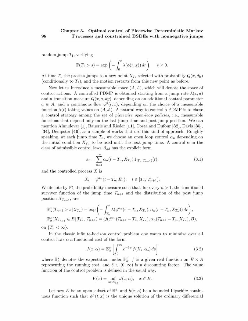
I.4. Optimal control of PDMPs. In Chapter 3 we prove that the value functionin an infinite-horizon optimal control problem for piecewise deterministic Markovprocesses (PDMPs) can be represented by means of an appropriate constrainedBSDE. As in Chapter 2, this is obtained by suitably extending the control ran-domization method in [88]. Compared to the pure jump case, the PDMPs contextis more involved and requires different techniques. In particular, the presence of thecontrolled flow in the PDMP’s dynamics and the corresponding differential operatorin the HJB equation suggest to use the theory of viscosity solutions. In addition,we consider discounted infinite-horizon optimal control problems, where the payoffis a cost to be minimized. Such problems are very traditional for PDMPs, see e.g.Davis [35], Costa and Dufour [32], Guo and Hernandez-Lerma [72]; moreover thefinite-horizon case can be brought back to the infinite-horizon case by means of astandard transformation, see Chapter 3 in [35]. The infinite-horizon character of theoptimal control problems complicates the tractation via the BSDE techniques, sinceit leads to deal with BSDEs over an infinite time horizon as well.
We consider controlled PDMPs on a general measurable state space (E,E). Theseprocesses are obtained starting from a continuous deterministic flow φβ(t, x), (t, x) ∈[0, ∞) × E, depending on the choice of a function β(t) taking values on the spaceof control actions (A,A), and from a jump rate λ(x, a) and a transition measureQ(x, a, dy) on E, depending both on (x, a) ∈ E × A. We select the control strategyamong the set of piecewise open-loop policies, i.e., measurable functions that dependonly on the last jump time and post jump position. This kind of approach is habitualin the literature, see for instance Almudevar [1], Davis [34], Bauerle and Rieder [11],Lenhart and Yamada [91], Dempster [40]. Roughly speaking, at each jump time Tn,we choose an open loop control αn depending on the initial condition XTn to be
14 Introduction
used until the next jump time. A control α in this class of admissible control laws,denoted by Aad, has the explicit form
αt =∞∑n=1
αn(t− Tn, XTn) 1[Tn, Tn+1)(t), (28)
and the controlled process X is
Xt = φαn(t− Tn, XTn), t ∈ [Tn, Tn+1).
For any x ∈ E and α ∈ Aad, Pxα indicates the probability measure such that, for everyn ≥ 1, the conditional survivor function of the jump time Tn+1 and the distributionof the post jump position XTn+1 on Tn <∞ are
where Exα indicates the expectation with respect to Pxα, f is a given real function onE × A representing the running cost, and δ ∈ (0, ∞) is a discounting factor. Weassume that λ and f are bounded functions, uniformly continuous, and Q is a Fellerstochastic kernel.
When E is an open subset of Rd, and h(x, a) is a bounded Lipschitz continu-ous function, φα(t, x) is defined as the unique solution of the ordinary differentialequation
x(t) = h(x(t), α(t)), x(0) = x ∈ E.In this case, according to Davis and Farid [36], under the compactness assumption forthe space of control actions A, the value function V is the unique continuous viscositysolution on [0, ∞)× E to the fully-nonlinear, integro-differential HJB equation
δv(x) = supa∈A
(h(x, a) · ∇v(x) + λ(x, a)
∫E
(v(y)− v(x))Q(x, a, dy)
)x ∈ E. (30)
Our main goal is to represent the value function V (x) by means of an appropriatebackward stochastic differential equation. To this end, we implement the controlrandomization method in the PDMPs framework. The first step consists in replacing,for any starting point x ∈ E, the state trajectory and the associated control process(Xs, αs) by an uncontrolled PDMP (Xs, Is). The process (X, I) takes values onE × A, and is constructed in a canonical way by assigning a new triplet of localcharacteristics. The compensator corresponding to (X, I) is the random measure
p(ds dy db) = λ0(db) δx(dy) ds+ λ(x, a)Q(x, a, dy) δa(db) ds.
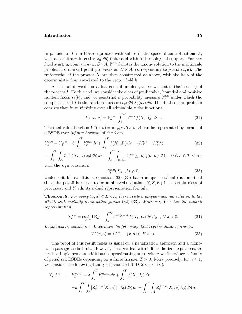
Introduction 15
In particular, I is a Poisson process with values in the space of control actions A,with an arbitrary intensity λ0(db) finite and with full topological support. For anyfixed starting point (x, a) in E×A, Px,a denotes the unique solution to the martingaleproblem for marked point processes on E × A, corresponding to p and (x, a). Thetrajectories of the process X are then constructed as above, with the help of thedeterministic flow associated to the vector field h.
At this point, we define a dual control problem, where we control the intensity ofthe process I. To this end, we consider the class of predictable, bounded and positiverandom fields νt(b), and we construct a probability measure Px,aν under which thecompensator of I is the random measure νs(db)λ0(db) ds. The dual control problemconsists then in minimizing over all admissible ν the functional
J(x, a, ν) = Ex,aν[∫ ∞
0e−δ s f(Xs, Is) ds
]. (31)
The dual value function V ∗(x, a) = infν∈V J(x, a, ν) can be represented by means ofa BSDE over infinite horizon, of the form
Y x,as = Y x,a
T − δ∫ T
sY x,ar dr +
∫ T
sf(Xr, Ir) dr − (Kx,a
T −Kx,as ) (32)
−∫ T
s
∫AZx,ar (Xr, b)λ0(db) dr −
∫ T
s
∫E×A
Zx,ar (y, b) q(dr dy db), 0 6 s 6 T <∞,
with the sign constraint
Zx,as (Xs−, b) > 0. (33)
Under suitable conditions, equation (32)-(33) has a unique maximal (not minimalsince the payoff is a cost to be minimized) solution (Y, Z,K) in a certain class ofprocesses, and Y admits a dual representation formula.
Theorem 8. For every (x, a) ∈ E×A, there exists a unique maximal solution to theBSDE with partially nonnegative jumps (32)-(33). Moreover, Y x,a has the explicitrepresentation:
Y x,as = ess inf
ν∈VEx,aν
[∫ ∞s
e−δ(r−s) f(Xr, Ir) dr∣∣∣Fs] , ∀ s > 0. (34)
In particular, setting s = 0, we have the following dual representation formula:
V ∗(x, a) = Y x,a0 , (x, a) ∈ E ×A. (35)
The proof of this result relies as usual on a penalization approach and a mono-tonic passage to the limit. However, since we deal with infinite-horizon equations, weneed to implement an additional approximating step, where we introduce a familyof penalized BSDEs depending on a finite horizon T > 0. More precisely, for n ≥ 1,we consider the following family of penalized BSDEs on [0, ∞):
Y n,x,as = Y n,x,a
T − δ∫ T
sY n,x,ar dr +
∫ T
sf(Xr, Ir) dr
−n∫ T
s
∫A
[Zn,x,ar (Xr, b)]− λ0(db) dr −
∫ T
s
∫AZn,x,ar (Xr, b)λ0(db) dr
16 Introduction
−∫ T
s
∫E×A
Zn,x,ar (y, b) q(dr dy db), 0 6 s 6 T <∞, (36)
where [z]− = max(−z, 0) denotes the negative part of z. In order to study the well-posedness of equation (36), we introduce a second family of penalized BSDEs, alsoparametrized by T > 0, and with zero final cost:
Y T,n,x,as = −δ
∫ T
sY T,n,x,ar dr +
∫ T
sf(Xr, Ir) dr
− n∫ T
s
∫A
[ZT,n,x,ar (Xr, b)]− λ0(db) dr
−∫ T
s
∫AZT,n,x,ar (Xr, b)λ0(db) dr
−∫ T
s
∫E×A
ZT,n,x,ar (y, b) q(dr dy db), 0 6 s 6 T. (37)
The existence of a unique solution (Y T,n, ZT,n) to (37) is a well known fact, and reliesas usual on fixed point arguments. We prove that the sequence (Y T )T>0 convergesPx,a-a.s. to some process Y , uniformly on compact subsets of R+, and that, for anyS > 0, the sequence (Zn,T |[0, S])T>S converges to some process Zn|[0, S] in a suitablesense. This allows to pass to the limit in (37), and, the time S being arbitrary, toconclude that (Y n, Zn) is the unique solution to (36). The process Y n satisfies thedual representation formula:
Y n,x,as = ess inf
ν∈VnEx,aν
[∫ ∞s
e−δ (r−s) f(Xr, Ir) dr∣∣∣Fs] , s > 0, (38)
where Vn denotes the subset of controls ν bounded by n.
By (38) we see that (Y n)n increasingly converges to Y as n goes to infinity.Moreover we provide uniform estimates on (Zn|[0, S],K
n|[0, S])n for every S > 0.Then we monotonically pass into the limit in (36) and we get the existence of the(unique) maximal solution (Y, Z,K) to the constrained BSDE (32)-(33), for whichwe also prove the dual representation formula (34).
Finally, we show that the maximal solution to (32)-(33) at the initial time alsoprovides a Feynman-Kac representation of the value function (29) of our originaloptimal control problem for PDMPs. To this end we introduce the deterministicreal function on E ×A
v(x, a) := Y x,a0 . (39)
We have the following result.
Theorem 9. The function v in (39) does not depend on the variable a:
v(x, a) = v(x, a′), ∀a, a′ ∈ A,
for all x ∈ E. Let us define
v(x) = v(x, a), ∀x ∈ E,
for any a ∈ A. Then v is a viscosity solution to (30).
Introduction 17
Notice that the concept of viscosity solution we use does not require continuityproperties; this is usually called discontinuous viscosity solution.
The fact that the function v in (39) is independent on its last component (whichis a consequence of the A-nonnegative constrained jumps) has a key role in thederivation of the viscosity solution properties of v, and the proof of this featureconstitutes a relevant task. Differently from [88] and the related papers in thediffusive context, this is obtained exclusively by means of control-theoretic techniquesand relies on the identification formula (35). By avoiding the use of viscosity theorytools, no additional hypothesis is required on the space of controls A, which cantherefore be very general. The non-dependence of v on a is a consequence of thefollowing result.
Proposition 10. Fix x ∈ E, a, a′ ∈ A, and ν ∈ V. Then, there exists a sequence(νε)ε ∈ V such that
limε→0+
J(x, a′, νε) = J(x, a, ν). (40)
Indeed identity (40) implies that V ∗(x, a′) ≤ J(x, a, ν), for every x ∈ E, a, a′ ∈ A.By the arbitrariness of ν it follows that
V ∗(x, a′) ≤ V ∗(x, a)
and, exchanging the roles of a and a′, this allows to conclude that V ∗(x, a) = v(x, a)does not depend on a.
Once we get that V ∗ (and therefore v) does not depend on a, we show that itactually provides a viscosity solution to the HJB equation (30). Differently to theprevious literature, we give a direct proof of the viscosity solution property of v,which avoid to resort to a penalized HJB equation. This is achieved by generalizingto the setting of the dual control problem the classical proof that allows to derivethe HJB equation from the dynamic programming principle. As a preliminary step,we need to give an identification result of the following form.
Lemma 11. The function v is such that, for any (x, a) ∈ E ×A, we have
Y x,as = v(Xs, Is), s > 0 dPx,a ⊗ ds -a.e. (41)
Identification (41) is proved by showing an analogous result for Y n, and usingthe convergence of Y n to Y provided in Theorem 8. This result follows from theMarkov property of the state process (X, I), and relies on an iterative constructionof the solution of standard BSDEs inspired by El Karoui, Peng and Quenez [53].
Finally, to conclude that v(x) actually gives the unique solution to the HJBequation we need to use a comparison theorem for viscosity sub and supersolutionsto the equation (30). Under an additional assumption on λ and Q (see condition(HλQ’)), and the compactness of A, the above mentioned comparison theoreminsures that v is the unique viscosity solution to (30), which coincides therefore tothe value function V . This yields in particular the nonlinear Feynman-Kac formulafor V , as well as the equality between the value functions of the primal and the dualcontrol problems.
18 Introduction
Corollary 12. Assume that A is compact, and that Hypothesis (HλQ’) holds. Thenthe value function V of the optimal control problem defined in (29) admits the non-linear Feynman-Kac representation formula:
V (x) = Y x,a0 , (x, a) ∈ E ×A.
Moreover, V (x) = V ∗(x, a).
II. BSDEs driven by general random measures, possibly nonquasi-left continuous
As we have already mentioned, BSDEs with discontinuous driving terms havebeen considered by many authors, among which Barles, Buckdahn and Pardoux [10],El Karoui and Huang [50], Xia [131], Becherer [12], Carbone, Ferrario, Santacroce[22], Cohen and Elliott [26], Jeanblanc, Mania, Santacroce and Schweizer [80], Con-fortola, Fuhrman and Jacod [29]. In all the papers cited above, and more generallyin the literature on BSDEs, the generator of the backward stochastic differentialequation, usually denoted by f , is integrated with respect to a measure dA, whereA is a nondecreasing continuous (or deterministic and right-continuous as in [26])process. In Chapter 4 we provide an existence and uniqueness result for the generalcase, i.e. when A is a right-continuous nondecreasing predictable process..
More precisely, consider a finite horizon T > 0, a Lusin space (E,E) and a filteredprobability space (Ω,F, (Ft)t≥0,P), with (Ft)t≥0 right continuous. We denote by P
the predictable σ-field on Ω× [0, T ]. In Chapter 4 we study the backward stochasticdifferential equation
Yt = ξ+
∫(t,T ]
f(s, Ys−, Zs(·)) dAs−∫
(t,T ]
∫EZs(x) (µ−ν)(ds, dx), 0 ≤ t ≤ T, (42)
where µ is an integer valued random measure on R+×E with compensator ν(dt, dx) =dAt φt(dx), with A a right-continuous nondecreasing predictable process such thatA0 = 0, and φ is a transition probability from (Ω× [0, T ],P) into (E,E). We suppose,without loss of generality, that ν satisfies ν(t×dx) ≤ 1 identically, so that ∆At ≤ 1.
For such general BSDE the existence and uniqueness results were at disposalonly in particular frameworks, see e.g. [26] for the deterministic case, and counter-examples were provided in the general case, see Section 4.3 in [29]. For this reason,the existence and uniqueness result is not a trivial extension of known results, andwe have to impose an additional technical assumption, which is of course violatedby the counter-example presented in [29].
Let us give some definitions. For any β ≥ 0, Eβ denotes the Doleans-Dadeexponential of the process βA, namely
Eβt = eβ At
∏0<s≤t
(1 + β∆As) e−β∆As . (43)
Introduction 19
By H2β(0, T ) we indicate the set of pairs (Y, Z) such that Y : Ω × [0, T ] → R is an
adapted cadlag process satisfying
‖Y ‖2H2β,Y (0,T ) := E
[ ∫(0,T ]
Eβt |Yt−|2 dAt
]<∞, (44)
and Z : Ω× [0, T ]× E → R is a predictable random field satisfying
‖Z‖2H2β,Z(0,T ) := E
[ ∫(0,T ]
Eβt
∫E
∣∣Zt(x)− Zt∣∣2 ν(dt, dx)
+∑
0<t≤TEβt
∣∣Zt∣∣2(1−∆At)]
< ∞, (45)
where
Zt =
∫EZt(x) ν(t × dx), 0 ≤ t ≤ T.
Definition 13. A solution to equation (42) with data (β, ξ, f) is a pair (Y,Z) ∈H2β(0, T ) satisfying equation (42). We say that equation (42) admits a unique solu-
tion if, given two solutions (Y,Z), (Y ′, Z ′) ∈ H2β(0, T ), we have (Y,Z) = (Y ′, Z ′) in
H2β(0, T ).
Notice that, given a solution (Y,Z) to equation (42) with data (β, ξ, f), theprocess (Zt1[0,T ](t))t≥0 belongs to the space G2(µ) introduced in Jacod’s book [77].
In particular, the stochastic integral∫
(t,T ]
∫E Zs(x) (µ − ν)(ds, dx) in (42) is well-
defined, and the process Mt :=∫
(0,t]
∫E Zs(x)(µ − ν)(ds, dx), t ∈ [0, T ], is a square
integrable martingale.
Suitable measurability and integrability conditions are imposed on ξ and on f ,and f is also asked to verify a uniform Lipschitz condition of the form:
|f(ω, t, y′, ζ ′)− f(ω, t, y, ζ)| ≤ Ly|y′ − y|
+ Lz
(∫E
∣∣∣∣ζ ′(x)− ζ(x)−∆At(ω)
∫E
(ζ ′(z)− ζ(z)
)φω,t(dz)
∣∣∣∣2 φω,t(dx)
+ ∆At(ω)(1−∆At(ω)
)∣∣∣∣ ∫E
(ζ ′(x)− ζ(x))φω,t(dx)
∣∣∣∣2)1/2
, (46)
for some Ly, Lz ≥ 0. As usual, in order to prove the well-posedness of the BSDE (42)we give a preliminary result, where the existence and uniqueness of the equation isprovided where f does not depend on (y, ζ).
Lemma 14. Consider a triple (β, ξ, f) and suppose that f = f(ω, t) does not dependon (y, ζ). Then, there exists a unique solution (Y,Z) ∈ H2
β(0, T ) to equation (42)
with data (β, ξ, f). Moreover, the following identity holds:
E[Eβt |Yt|2
]+ β E
[ ∫(t,T ]
Eβs (1 + β∆As)−1 |Ys−|2 dAs
]+ E
[ ∫(t,T ]
Eβs
∫E
∣∣Zs(x)− Zs∣∣2 ν(ds, dx) +
∑t<s≤T
Eβs∣∣Zs∣∣2(1−∆As
)]
20 Introduction
= E[EβT |ξ|
2]
+ 2E[ ∫
(t,T ]Eβs Ys− fs dAs
]− E
[ ∑t<s≤T
Eβs |fs|2 |∆As|2], (47)
for all t ∈ [0, T ].
The proof of Lemma 14 is based on the martingale representation theorem formarked point processes given in [75]. In order to prove the existence and uniquenessresults we take into account that Mt :=
∫(t, T ]
∫E Zs(y) (µ − ν)(ds dy) is a square
integrable martingale if and only if Z ∈ G2loc(µ), and that
〈M,M〉T =
∫(0,T ]
∫E
∣∣Zt(x)− Zt∣∣2 ν(dt, dx) +
∑0<t≤T
∣∣Zt∣∣2(1−∆At),
see Theorem B.22). Properties of the Doleans-Dade exponential Eβ are also ex-
ploited, in particular we use that dEβs = β Eβs− dAs and that Eβs− = Eβs (1+β∆As)
−1.
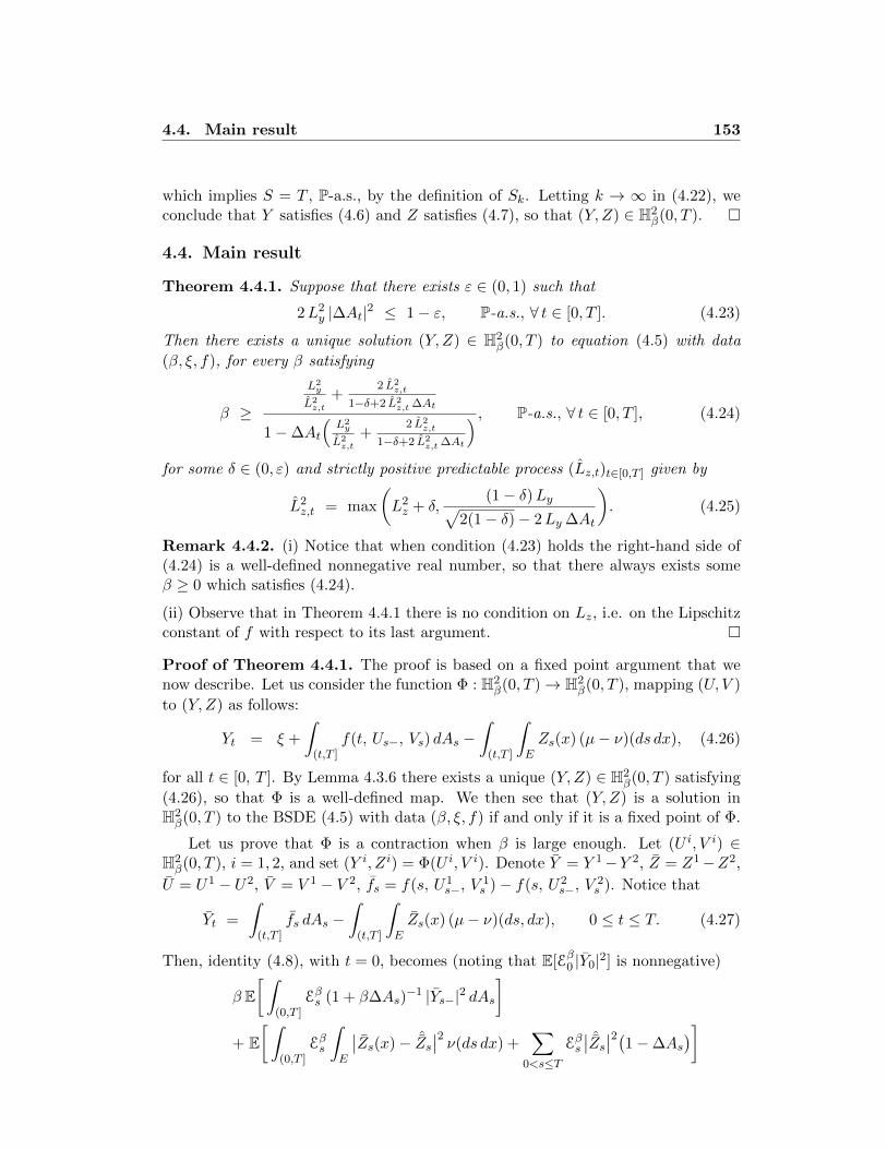
Identity (47) plays a fundamental role to get our main result, which reads asfollows.
Theorem 15. Suppose that there exists ε ∈ (0, 1) such that
2L2y |∆At|2 ≤ 1− ε, P-a.s., ∀ t ∈ [0, T ]. (48)
Then there exists a unique solution (Y, Z) ∈ H2β(0, T ) to equation (42) with data
(β, ξ, f), for every β such that
β ≥ βt P-a.s., ∀ t ∈ [0, T ],
where (βt)t∈[0, T ] is a strictly positive predictable process depending only on ε, ∆A,Lz and Ly.
The proof of Theorem 15 is based on Lemma 14, and is quite technical. Noticethat in [26] the same condition (48) is imposed. As mentioned earlier, in that paperthe authors study a class of BSDEs with a generator f integrated with respect toa deterministic (rather than predictable) right-continuous nondecreasing process A,and provide an existence and uniqueness result for this class of BSDEs. However, theproof in [26] relies heavily on the assumption that A is deterministic, and can not beextended to the case where A is predictable, which therefore requires a completelydifferent procedure.
II.1. Motivation and future applications. The results in Theorem 15 couldbe employed to solve, by means of the BSDEs theory, optimal control problems ofPDMPs on state spaces with boundary. We recall that the BSDEs approach tooptimal control for PDMPs is implemented in Chapter 3 by means of the controlrandomization method. However, in that chapter only the case of PDMPs takingvalues in open state spaces is considered. Indeed in those cases the compensatorν(ds dy) = dAs φt(dy) of the random measure associated to the PDMP is quasi-left continuous, and a fairly complete theory was developed in the literature forBSDEs driven by such random measures. On the contrary, PDMP’s jumps at theboundary of the domain correspond to predictable discontinuities for the process A.BSDEs driven by random measures of this type belong to the class of equations (42)
Introduction 21
mentioned before, for which, to our knowledge, Theorem 15 constitutes the onlygeneral well-posedness result at disposal in literature.
More precisely, consider a PDMP X on a general state space E with boundary∂E. The jump dynamics of X in the interior of the domain is described by thetransition probability measureQ : E×E→ E and the jump rate measure λ : E → R+
introduced in Chapter 3. In addition, a forced jump occurs every time the processreaches the active boundary Γ ∈ ∂E (for the precise definition of Γ see page 61 in[35]). In this case, the process immediately jumps back to the interior of the domainaccordingly to a transition probability measure R : ∂E × E→ E. The compensatorof the integer-valued random measure associated to X then admits the form
p(ds dy) = λ(Xs−)Q(Xs−, dy) ds+R(Xs−, dy) dp∗s,
where
p∗s =∞∑n=1
1s≥Tn 1XTn−∈Γ
is the process counting the number of jumps of X from the active boundary Γ ∈ ∂E.In particular, the compensator can be rewritten as
p(ds dy) = dAs φ(Xs−, dy),
where φ(Xs−, dy) := Q(Xs−, dy) 1Xs−∈E +R(Xs−, dy) 1Xs−∈Γ, and
As := λ(Xs−) ds+ dp∗s
is a predictable and discontinuous process, with jumps ∆As = 1Xs−∈Γ.
In this context condition (48) in Theorem 15 reads
Ly <1√2. (49)
This is the only additional condition required in order to have a unique solution toa BSDE of the form (42) driven by the random measure associated to a PDMP. Inparticular, Theorem 15 does not impose any condition on Lz, i.e. on the Lipschitzconstant of f with respect to its last argument. This is particularly important in thestudy of control problems related to PDMPs by means of BSDEs methods: in thiscase indeed Ly = 0 and condition (49) is automatically satisfied. This fact opens tothe possibility of extending the control randomization method developed in Chapter3 also in the case of optimal control of PDMPs with bounded domain. This will bethe subject of a future work.
III. Weak Dirichlet processes and BSDEs driven by a randommeasure
III.1. State of the art. Stochastic calculus via regularization was essentially knownin the case of continuous integrators X, see e.g. Russo and Vallois [116], [117]. Asurvey on basic elements of the calculus, can be found in Russo and Vallois [121];it applies mainly in the case when X is not a semimartigale. In the framework ofcalculus via regularizations, a complete theory has been developed. In particularstochastic differential equations were studied, Ito formulae for processes with finite
22 Introduction
quadratic (and more general) variations were provided. In Flandoli and Russo [63]were given Ito-Wentzell type formulae, and generalizations to the case of Banachspace type integrators are considered for instance in Di Girolami and Russo [44].The notion of covariation [X,Y ] (resp. quadratic variation [X,X]) for two processesX,Y (resp. a process X) has been introduced in the framework of regularizations(see Russo and Vallois [119]) and of discretization as well (see Follmer [66]). Forinstance, if X is a finite quadratic variation continuous process, an Ito formula hasbeen proved for the expansion of F (Xt), when F ∈ C2, see [119]. When F is of classC1 and X a reversible semimartingale, an Ito expansion was established in Russoand Vallois [120]. An important notion in calculus via regularizations is the one ofDirichlet process (with respect to a given filtration (Ft)). The notion of Dirichletprocess is a generalization of the concept of semimartingale, and was introduced by[66] and Bertoin [14] in the discretization framework. The analogue of the Doob-Meyer decomposition for a Dirichlet process is that it is the sum of a local martingaleM and an adapted process A with zero quadratic variation. Here A is the general-ization of a bounded variation process. The concept of (Ft)-weak Dirichlet process(or simply weak Dirichlet process) was later introduced in Errami and Russo [58]and Gozzi and Russo [71] and applications to stochastic control were considered inGozzi and Russo [70]. Such a process is defined as the sum of a local martingale Mand an adapted (Ft)-orthogonal process A, in the sense that [A,N ] = 0 for everycontinuous local martingale N . An (Ft)-weak Dirichlet process constitutes a naturalgeneralization of the notion of the one of (Ft)-Dirichlet process. An useful chain rulewas established for F (t,Xt) when F belongs to class C0,1 and X is a weak Dirichletprocess (with finite quadratic variation), see [71]. Such a process is indeed again aweak Dirichlet process (with possibly no finite quadratic variation).
As far as calculus via regularizations when X is a cadlag integrator process only afew steps were done: we refer in particular to [119], Russo and Vallois [118], and thebook of Di Nunno, Øksendal and Proske [45], see Chapter 15 and references therein.For instance no Ito type formulae have been established and in the discretizationframework only few chain rule results are available for F (X), when F (X) is not asemimartingale. In that direction two peculiar results are available: the expansionof F (Xt) when X is a reversible semimartingale and F is of class C1 with someHolder conditions on the derivatives (see Errami, Russo and Vallois [59]) and achain rule for F (Xt) when X is a weak Dirichlet (cadlag) process and F is of classC1, see Coquet, Jakubowsky, Memin and Slominsky [30]. The work in [59] hasbeen continued by several authors, see e.g. Eisenbaum [47] and references therein,expanding the remainder making use of local time type processes.
In fact, the notion of (Ft)-Dirichlet process does not fit to the framework of cal-culus with respect to jump processes. Indeed, requiring a process A to be of zeroquadratic variation imposes that A is continuous. On the other hand, a boundedvariation process with jumps has a non zero finite quadratic variation, so the general-ization of the semimartingale is not necessarily represented by the notion of Dirichletprocess. The property of weak Dirichlet process turns out to be a correct general-ization of the one of semimartingale in the discontinuous framework. This concept
Introduction 23
was extended to the case of jumps processes in the significant work [30], by usingthe discretizations techniques.
III.2. Stochastic calculus via regularization and weak Dirichlet processeswith jumps. In Chapter 5 we extend, in a systematic way, stochastic calculus viaregularizations to the case of jump processes, and we carry on the investigations ofthe so called weak Dirichlet processes in the discontinuous case.
The first basic objective consists in developing a calculus via regularization inthe case of finite quadratic variation cadlag processes. To this end, we revisit thedefinitions given by [119] concerning forward integrals (resp. covariations). Let Xand Y be two cadlag processes. The stochastic integral
∫ ·0 Ys d
−Xs and the covari-ation [Y,X] are defined as the uniform convergence in probability (u.c.p.) limit ofthe expressions
I−ucp(ε, t, Y, dX) =
∫(0, t]
Y (s)X((s+ ε) ∧ t)−X(s)
εds, (50)
[Y,X]ucpε (t) =
∫(0, t]
(Y ((s+ ε) ∧ t)− Y (s))(X((s+ ε) ∧ t)−X(s))
εds. (51)
That convergence ensures that the limiting objects are cadlag, since the approxi-mating expressions have the same property. For instance a cadlag process X will becalled finite quadratic variation process whenever the limit (which will be denotedby [X,X]) of
[X,X]ucpε (t) :=
∫(0, t]
(X((s+ ε) ∧ t)−X(s))2
εds (52)
exists u.c.p. In [119], the authors introduced a slightly different approximation of[X,X] when X is continuous, namely
Cε(X,X)(t) :=
∫(0, t]
(X((s+ ε)−X(s))2
εds. (53)
When the u.c.p. limit of Cε(X,X) exists, it is automatically a continuous process,since the approximating processes are continuous. For this reason, when X is a jumpprocess, the choice of approximation (53) would not be suitable, since its quadraticvariation is expected to be a jump process. In that case, the u.c.p. convergence of(52) can be shown to be equivalent with a notion of convergence which is associatedwith the a.s. convergence (up to subsequences) in measure of Cε(X,X)(t) dt. Bothformulations will be used in the development of the calculus.
For a cadlag finite quadratic variation process X, we establish, via regularizationtechniques, an Ito formula for C1,2 functions of X of the following form.
Proposition 16. Let X be a finite quadratic variation cadlag process and F : [0, T ]×R→ R a function of class C1,2. Then
F (t,Xt) =F (0, X0) +
∫ t
0∂sF (s,Xs) ds+
∫ t
0∂xF (s,Xs) d
−Xs
24 Introduction
+1
2
∫ t
0∂2xxF (s,Xs−) d[X,X]cs
+∑s≤t
[F (s,Xs)− F (s,Xs−)− ∂xF (s,Xs−) ∆Xs]. (54)
From Proposition 16 will easily follow an Ito formula under weaker regularityconditions on F . Notice that a similar formula was stated in [59], using a discretiza-tion definition of the covariation, when F is time-homogeneous.
Proposition 17. Let F : [0, T ]×R→ R be a function of class C1 such that ∂xF isHolder continuous with respect to the second variable for some λ ∈ [0, 1). Let (Xt)be a reversible semimartingale, satisfying∑
0<s≤t|∆Xs|1+λ <∞ a.s.
Then
F (t,Xt) = F (0, X0) +
∫ t
0∂sF (s,Xs) ds+
∫ t
0∂xF (s,Xs−) dXs +
1
2[∂xF (·, X), X]t
+ J(F,X)(t),
where
J(F,X)(t) =∑
0<s≤t
[F (s,Xs)− F (s,Xs−)− ∂xF (s,Xs) + ∂xF (s,Xs−)
2∆Xs
].
The proof of Proposition 16 is based on an accurate separation between theneighborhood of ”big” and ”small” jumps, where specific tools are used. To thisend, a fundamental role is played by the two following lemmata, the second onebased on Lemma 1, Chapter 3, in Billingsley [16].
Lemma 18. Let Yt be a cadlag function with values in Rn. Let φ : Rn × Rn → Rbe a uniformly continuos function on each compact, such that φ(y, y) = 0 for everyy ∈ Rn. Let 0 ≤ t1 ≤ t2 ≤ ... ≤ tN ≤ T . We have
N∑i=1
1
ε
∫ ti
ti−ε1]0, s](t)φ(Y(t+ε)∧s, Yt) dt
ε→0−→N∑i=1
1]0, s](ti)φ(Yti , Yti−), (55)
uniformly in s ∈ [0, T ].
Lemma 19. Let X be a cadlag (caglad) real process. Let γ > 0, t0, t1 ∈ R andI = [t0, t1] be a subinterval of [0, T ] such that
|∆Xt|2 ≤ γ2, ∀t ∈ I. (56)
Then there is ε0 > 0 such that
supa, t∈I|a−t|≤ε0
|Xa −Xt| ≤ 3γ.
Another significant tool for our scopes is a Lemma of Dini type in the case ofcadlag functions, which reads as follows.
Introduction 25
Lemma 20. Let (Gn, n ∈ N) be a sequence of continuous increasing functions, letG (resp. F ) from [0, T ] to R be a cadlag (resp. continuous) function. We setFn = Gn +G and suppose that Fn → F pointwise. Then
lim supn→∞
sups∈[0, T ]
|Fn(s)− F (s)| ≤ 2 sups∈[0, T ]
|G(s)|.
The second target of the chapter consists in investigating weak Dirichlet jumpprocesses. Contrarily to the continuous case, the decomposition X = M + A isgenerally not unique. We introduce the notion of a special weak Dirichlet processwith respect to some filtration (Ft). Such a process is a weak Dirichlet processadmitting a decomposition
X = M c +Md +A, (57)
whereM c is a continuous local martingale, Md is a purely discontinuous local martin-gale, and A is an (Ft)-orthogonal, predictable process. Supposing that A0 = Md
0 = 0,the decomposition (57) is unique. In that case the decomposition (57) will be calledthe canonical decomposition of X. We remark that a continuous weak Dirichletprocess is special weak Dirichlet.
In the sequel we will denote by µX the jump measure associated to X, and by νX
its compensator. We will also indicate by Ducp the set of all adapted cadlag processesequipped with the topology of the uniform convergence in probability (u.c.p.), byA (resp Aloc) the collection of all adapted processes with integrable variation (resp.with locally integrable variation), and by A+ (resp A+
loc) the collection of all adaptedintegrable increasing (resp. adapted locally integrable) processes.
We start by giving an expansion of F (t,Xt) where F is of class C0,1 and X isa cadlag weak Dirichlet process of finite quadratic variation. The process (F (t,Xt))turns out to be again a weak Dirichlet process, however not necessarily of finitequadratic variation.
Theorem 21. Let X = M +A be a cadlag weak Dirichlet process of finite quadraticvariation. Then, for every F : [0, T ]× R→ R of class C0,1, we have
(F (s,Xs− + x)− F (s,Xs−)− x ∂xF (s,Xs−)) 1|x|>1 µX(ds dx) + ΓF (t),
where ΓF : C0,1 → Ducp is a continuous linear map, such that, for every F ∈ C0,1,it fulfills the following properties.
(a) [ΓF , N ] = 0 for every N continuous local martingale.
(b) If A is predictable, then ΓF is predictable.
26 Introduction
Starting from Theorem 21, we are able to provide an analogous chain rule whenX and (F (t,Xt)) are both special weak Dirichlet processes. This constitutes ourmain result. We make use of the following conditions.∫
(0,·]×R|F (t,Xt− + x)− F (t,Xt−)− x ∂xF (t,Xt−)| 1|x|>1 µ
X(dt dx) ∈ A+loc, (59)∫
(0,·]×R|x| 1|x|>1 µ
X(dt dx) ∈ A+loc. (60)
Theorem 22. Let X be a special weak Dirichlet process of finite quadratic variationwith its canonical decomposition X = M c + Md + A. Assume that condition (59)holds. Then, for every F : [0, T ]× R→ R of class C0,1, we have
(1) Yt = F (t,Xt) is a special weak Dirichlet process, with decomposition Y =MF +AF , where
MFt = F (0, X0) +
∫ t
0∂xF (s,Xs) d(M c +Md)s
+
∫(0, t]×R
(F (s,Xs− + x)− F (s,Xs−)− x ∂xF (s,Xs−)) (µX − νX)(ds dx),
and AF : C0,1 → Ducp is a linear map such that, for every F ∈ C0,1, AF isa predictable (Ft)-orthogonal process.
(2) If in addition condition (60) holds, MF reduces to
MFt = F (0, X0) +
∫ t
0∂xF (s,Xs) dM
cs
+
∫(0, t]×R
(F (s,Xs− + x)− F (s,Xs−)) (µX − νX)(ds dx).
We remark that a first important step in this sense was done in [30], where Xbelongs to a bit different class of special weak Dirichlet jump processes (of finiteenergy) and F does not depend on time and has bounded derivative. In [30] theauthors show that F (X) is again a special weak Dirichlet process. There the un-derlying process has finite energy, which requires a control of the expectation of theapproximating sequences of the quadratic variation. On the other hand, our tech-niques do not require that type of control. Moreover, the integrability condition (59)that we ask on F (t,Xt) in order to get the chain rule in Theorem 22 is automaticallyverified under the hypothesis on the first-order derivative considered in [30].
In some circumstances a chain rule may hold even when F is only continuous ifwe know a priori some information of (F (t,Xt)). No assumption are required in thiscase on the cadlag process X.
Proposition 23. Let X be an adapted cadlag process. Let F : [0, T ]× R → R be acontinuous function such that the following holds.
(i) F (t,Xt) = Bt +A′t, where B has bounded variation and A′ is a continuous(Ft)-orthogonal process;
Then F (t,Xt) is a special weak Dirichlet process with decomposition
F (t,Xt) = F (0, X0)+
∫(0, t]×R
(F (s,Xs−+x)−F (s,Xs−)) (µX −νX)(ds dx)+AF (t),
(61)where AF is a predictable (Ft)-orthogonal process.
Finally, we also introduce a subclass of weak Dirichlet processes, called partic-ular. A particular weak Dirichlet process X admits a decomposition X = M + A,where M is an (Ft)-local martingale, and A = V + A′, with V a bounded variationadapted process and A′ a continuous adapted process (Ft)-orthogonal process suchthat A′0 = 0. Those processes inherit some of the semimartingales features: as inthe semimartingale case, the particular weak Dirichlet processes admit a (unique)canonical decomposition when
∫(0, ·]×R |x| 1|x|>1 µ(dt dx) ∈ A+
loc. and an integral
representation holds. Under that condition, those particular processes are indeedspecial weak Dirichlet processes.
III.3. Application to BSDEs driven by a random measure. In Chapter 6we apply the stochastic calculus developed in Chapter 5, and we provide an identifi-cation result for the solution of a forward backward stochastic differential equationdriven by a random measure, when the underlying process X is of weak Dirichlettype. Indeed, given a solution (Y,Z, U) to this forward BSDE, often Y appears tobe of the type u(t,Xt) where u is a deterministic function; by using the stochasticcalculus with respect to weak Dirichlet processes, we are able to identify also Z andU in terms of u.
More precisely, fix a finite time horizon T > 0 and let (Ω,F, (Ft)t≥0,P) be a givenfiltered probability space, where (Ft)t≥0 satisfies the usual conditions. We will focuson general BSDEs of the type
Yt = ξ +
∫(t, T ]
g(s, Ys−, Zs) dζs +
∫(t, T ]×R
f(s, e, Ys−, Us(e))λ(ds de)
−∫
(t, T ]Zs dMs −
∫(t, T ]×R
Us(e) (µ− ν)(ds de). (62)
Here µ is a random measure on [0, T ] × R with compensator ν. Besides µ and νappear three driving random elements: a continuous martingale M , a non-decreasingadapted continuous process ζ, and a predictable random measure λ on [0, T ] × R,equipped with the usual product σ-fields. The other data of equation (62) are asquare integrable random variable ξ, and two measurable functions g : Ω × [0, T ] ×R2 → R, f : Ω× [0, T ]× R3 → R.
The Brownian context of Pardoux-Peng [99] appears as a particular case, settingµ = λ = 0, ζs ≡ s. There M is a standard Brownian motion and ξ is measurablewith respect to the Brownian σ-field at terminal time. In that case the unknowncan be reduced to (Y,Z), since U can be arbitrarily chosen. Another importantsubcase of (62) arises when only the purely discontinuous driving term appears,i.e. M and ζ vanish. A significant example is represented by BSDEs driven by the
28 Introduction
random measure associated to a pure jump process, as in Chapter 2, or to a piecewisedeterministic Markov process, as in Chapter 3.
When the random dependence of f and g is provided by a Markov solution X ofa forward SDE, and ξ is a real function of X at the terminal time T , equation (62)becomes a forward BSDE. As we have recalled in Section I, this generally constitutesa stochastic representation of a partial integro-differential equation (PIDE). Indeed,solutions of forward BSDEs generate solutions of PIDEs in the viscosity sense. Moreprecisely, for each given couple (t, x) ∈ [0, T ]×R, consider an underlying process Xgiven by the solution Xt,x of an SDE starting at x at time t. Let (Y t,x, Zt,x, U t,x)be a family of solutions of the forward BSDE. In that case, under reasonable generalassumptions, the function v(t, x) := Y t,x
t is a viscosity solution of the related PIDE.A demanding task consists in characterizing the pair (Z,U) := (Zt,x, U t,x), in term ofv; this is generally called the identification problem of (Z,U). In the continuous case,this was for instance the object of Fuhrman and Tessitore [68]: the authors showthat if v ∈ C0,1, then Zs = ∂xv(s,Xs); under more general assumptions, they alsoassociate Z with a generalized gradient of v. At our knowledge, in the discontinuouscase, the problem of the identification of the martingale integrands pair (Z,U) hasnot been deeply investigated, except for particular situations, as for instance thepurely discontinuous case treated in Confortola and Fuhrman [28].
In Chapter 6 we discuss the mentioned identification problem in a quite generalframework by means of the calculus related to weak Dirichlet processes. When Y isa deterministic function v of a special semimartingale X (or more generally a specialweak Dirichlet process with finite quadratic variation), related in a specific way tothe random measure µ, we apply the chain rule in Theorem 22 in order to identifythe pair (Z,U).
We fix an integer-valued random measure µ on [0, T ]× R, with compensator ν.We suppose, without loss of generality, that ν satisfies ν(t × dx) ≤ 1 identically.We set
D = (ω, t) : µ(ω, t × R) > 0,J = (ω, t) : ν(ω, t × R) > 0,K = (ω, t) : ν(ω, t × R) = 1.
We will ask the following condition on µ.
Hypothesis 24.
(i) D = K ∪ (∪n[[T in]]) up to an evanescent set, where (T in)n are totally inac-cessible times such that [[T in]] ∩ [[T im]] = ∅, n 6= m.
(ii) For every predictable time S such that [[S]] ⊂ K, ν(S, de) = µ(S, de)a.s.
With respect to a generic process X, we will consider the following assumptionin relation to µ.
Hypothesis 25. X = Xi +Xp, where Xp is a cadlag predictable process satisfying∆Xp 6= 0 ⊂ J , and Xi is a cadlag quasi-left continuous adapted process satisfying
Introduction 29
∆Xi 6= 0 ⊂ D. Moreover, there exists a predictable measurable map γ : Ω×]0, T ]×R→ R such that
The hypothesis below will concern a pair of processes (X,Y ).
Hypothesis 26. X is a special weak Dirichlet process of finite quadratic variation,satisfying condition (60). Yt = v(t, Xt) for some (deterministic) function v : [0, T ]×R→ R of class C0,1 such that F = v and X verify condition (59).
We have the following result.
Proposition 27. Let µ satisfy Hypothesis 24. Let X be a process verifying Hypoth-esis 25 with decomposition X = Xi + Xp, where γ is the predictable process whichrelates µ and Xi in agreement with (63). Let (Y, Z, U) be a solution to the BSDE(62) such that the pair (X,Y ) satisfies Hypothesis 26 with corresponding functionv. Let Xc denote the continuous local martingale M c of X given in the canonicaldecomposition (57). If Us − (v(s,Xs− + γ(s, ·))− v(s,Xs−)) ∈ G2
loc(µ), then the pair(Z,U) fulfills
Zs = ∂xv(s,Xs)d〈Xc,M〉sd〈M〉s
dP d〈M〉s -a.e., (64)
Us − (v(s,Xs− + γ(s, ·))− v(s,Xs−)) = ls 1K(s) dP ν(ds de)-a.e., (65)
where l is a predictable process.
In the purely discontinuous framework, i.e. when in the BSDE (62) M and ζvanish, we make use of the chain rule (61) in Proposition 23, which allows, for ageneral cadlag process X, to express v(t,Xt) without requiring any differentiabilityon v. In particular Proposition 23 does not ask X to be a special weak Dirichletprocess, provided we have some a priori information on the structure of v(t,Xt). Weneed the following condition on a pair of processes (X,Y ).
Hypothesis 28.
(i) Y = B + A′, with B a bounded variation process and A′ a continuous(Ft)-orthogonal process;
(ii) Yt = v(t, Xt) for some continuous deterministic function v : [0, T ]×R→ R,satisfying the integrability condition∫
(0, ·]×R|v(t,Xt− + x)− v(t,Xt−)|µX(dt dx) ∈ A+
loc. (66)
The identification in that case reads as follows.
Proposition 29. Let µ satisfy Hypothesis 24. Let X verify Hypothesis 25 withdecomposition X = Xi +Xp, where γ is the predictable process which relates µ andXi in agreement with (63). Let (Y,U) be a solution to the BSDE (62) with M = 0and ζ = 0, such that (X,Y ) satisfies Hypothesis 28 with corresponding function v.
30 Introduction
If in addition Us − (v(s,Xs− + γ(s, ·)) − v(s,Xs−)) ∈ G2loc(µ), then there exists a
predictable process ls such that
Us − (v(s,Xs− + γ(s, ·))− v(s,Xs−)) = ls 1K(s) dP ν(ds de)-a.e. (67)
We remark that in most of the literature on BSDEs, the measures ν, λ and ζof equation (62) are non-atomic in time. As we have underlined in Chapter 4, achallenging case arises when one or more of those predictable processes have jumpsin time. Our approach to the identification problem also applies to forward BSDEspresenting predictable jumps. As an example, we provide an identification result fora BSDE driven by the random measure µ associated to a PDMP taking values in abounded real interval.
Further remarks and future developments of the thesis
We take the occasion to emphasize that every proof reported in the thesis is new;on the other hand, when a known result is needed, we give references to where aproof can be found. We also underline that Chapter 1 is based on Bandini andConfortola [4], Chapter 2 on Bandini and Fuhrman [7], Chapter 3 on Bandini [3],Chapter 4 on Bandini [2], Chapters 5 and 6 respectively on Bandini and Russo[9] and [8].
Some challenging issues arising in this work are left for future research. First ofall, as recalled in Section II.1, our existence and uniqueness result for BSDEs drivenby general, possibly non quasi-left continuous, random measures opens to the pos-sibility of studying optimal control problems for PDMPs with bounded state spacesby means of BSDEs techniques. This could allow to provide nonlinear Feynman-Kac representation formulae for the value functions of those control problems. Inparticular, combining ideas from Chapters 3 and 4, it might turn out that the valuefunction of the optimal control problem of a PDMP with a bounded state space solvesa backward stochastic differential equation with constrained jumps. Notice that itwould be interesting to apply to this context the identification results obtained inChapter 6, which are already conceived for BSDEs driven by random measures withpossible predictable jumps. Another challenging development might consist in ex-tending the results obtained in Chapter 2 to a non-Markovian pure jump framework.Optimal control problems for non-Markovian stochastic differential equations drivenby a Brownian motion have been recently studied with the BSDEs techniques bymeans of the control randomization approach, see Fuhrman and Pham [67]. In thiscontext the constrained BSDE characterizing the value function can be seen as apath-dependent version of the HJB equation. Notice that the control randomizationmethod does not rely on the path-dependent HJB equation associated by dynamicprogramming principle to the value function in the non-Markovian context. Thisallows to circumvent delicate issues of dynamic programming (as originally studiedin El Karoui [49] for general non-Markovian stochastic control problems), viscositysolutions and comparison principles for fully nonlinear path-dependent PDEs, as re-cently studied in Peng [106], Ekren, Keller, Touzi and Zhang [48] and Tang andZhang [127], see also Fabbri, Gozzi and Swiech [61] for HJB equations in infinite
Introduction 31
dimension arising typically for stochastic systems with delays. This suggests in par-ticular an original approach to derive the HJB equation for the value function ofstochastic control problem from the BSDE representation, hence without dynamicprogramming principle. The generalization of these results to the jump case has notyet been investigated, and could be obtained by mixing the methodology in [67] withthe specific theory for optimal control of pure jump processes developed in Chapter2. Finally, we emphasize that the chain rule type expansions provided in Chapter5 may be helpful to get verification theorems for stochastic optimal control prob-lems of general jump processes. In the diffusive context, this was done in Gozzi andRusso [70] which treated optimal control problems of continuous processes withoutcontrol in the diffusion. Those verification theorems have the advantage of requiringless regularity of the value function than the classical ones, which need instead C1
regularity in time and C2 in space (see e.g. Fleming and Soner [65]), and they canbe applied also to problems with pathwise optimality and optimality in probabil-ity. It would be also judicious to generalize our results of Chapters 5 and 6 to thecase of path-dependent cadlag processes. In the case of path-dependent continuousprocesses, a first step for extending the chain rules of Chapter 5 was done in [43].
Chapter 1
Optimal control ofsemi-Markov processeswith a BSDE approach
1.1. Introduction
In this chapter we study optimal control problems for a class of semi-Markovprocesses using a suitable class of backward stochastic differential equations, drivenby the random measure associated to the semi-Markov process itself.
Let us briefly describe our framework. Our starting point is a semi-Markov purejump process X on a general state space E. It is constructed starting from a jumprate function λ(x, ϑ) and a jump measure A 7→ Q(x, ϑ,A) on E, depending on x ∈ Eand ϑ ≥ 0. Our approach is to consider a semi-Markov pure jump process as a twodimensional time-homogeneous and strong Markov process (Xs, θs), s ≥ 0 with itsnatural filtration F and a family of probabilities Px,ϑ for x ∈ E, ϑ ∈ [0,∞) such thatPx,ϑ(X0 = x, θ0 = ϑ) = 1. If the process starts from (x, ϑ) at time t = 0 then thedistribution of its first jump time T1 under Px,ϑ is described by the formula
Px,ϑ(T1 > s) = exp
(−∫ ϑ+s
ϑλ(x, r) dr
), (1.1)
and the conditional probability that the process is in A immediately after a jump attime T1 = s is
Px,ϑ(XT1 ∈ A |T1 = s) = Q(x, s,A).
Xs is called the state of the process at time s, and θs is the duration period in thisstate up to moment s:
θs =
θ0 + s ifXp = Xs ∀ 0 6 p 6 s, p, s ∈ R,s− sup p : 0 6 p 6 s, Xp 6= Xs otherwise.
We note that X alone is not a Markov process. We limit ourselves to the caseof a semi-Markov process X such that the survivor function of T1 under Px,0 is
33
34Chapter 1. Optimal control of semi-Markov processes with a BSDE
approach
absolutely continuous and admits a hazard rate function λ as in (1.1). The holdingtimes of the process are not necessarily exponentially distributed and can be infinitewith positive probability. Our main restriction is that the jump rate function λ isuniformly bounded, which implies that the process X is non explosive. Denoting byTn the jump times of X, we consider the marked point process (Tn, XTn) and theassociated random measure p(dt dy) =
∑n δ(Tn,XTn ) on (0,∞)×E, where δ denotes
the Dirac measure. The dual predictable projection p of p (shortly, the compensator)has the following explicit expression
p(ds dy) = λ(Xs−, θs−)Q(Xs−, θs−, dy) ds.
In Section 1.3 we address an optimal intensity-control problem for the semi-Markov process. This is formulated in a classical way by means of a change ofprobability measure, see e.g. El Karoui [49], Elliott [57] and Bremaud [18]. Wedefine a class A of admissible control processes (us)s∈[0, T ]; for every fixed t ∈ [0, T ]and (x, ϑ) ∈ E × [0,∞), the cost to be minimized and the corresponding valuefunction are
J(t, x, ϑ, u(·)) = Ex,ϑu,t[∫ T−t
0l(t+ s,Xs, θs, us) ds+ g(XT−t, θT−t)
],
v(t, x, ϑ) = infu(·)∈A
J(t, x, ϑ, u(·)),
where g, l are given real functions. Here Ex,ϑu,t denotes the expectation with respect
to another probability Px,ϑu,t , depending on t and on the control process u and con-
structed in such a way that the compensator under Px,ϑu,t equals r(t+s,Xs−, θs−, y, us)λ(Xs−, θs−) Q(Xs−, θs−, dy) ds, for some function r given in advance as another da-tum of the control problem. Since the process (Xs, θs)s≥0 we want to control istime-homogeneous and starts from (x, ϑ) at time s = 0, we introduce a temporaltranslation which allows to define the cost functional for all t ∈ [0, T ]. For moredetails see Remark 1.3.2.
Our approach to this control problem consists in introducing a family of BSDEsparametrized by (t, x, ϑ) ∈ [0, T ]× E × [0,∞):
Y x,ϑs,t +
∫ T−t
s
∫EZx,ϑσ,t (y) q(dσ dy)
= g(XT−t, θT−t) +
∫ T−t
sf(t+ σ,Xσ, θσ, Z
x,ϑσ,t (·)
)dσ, (1.2)
s ∈ [0, T − t], where the generator is given by the Hamiltonian function f definedfor every s ∈ [0, T ], (x, ϑ) ∈ E × [0, +∞), z ∈ L2(E,E, λ(x, ϑ)Q(x, ϑ, dy)), as
f(s, x, ϑ, z(·)) = infu∈U
l(s, x, ϑ, u) +
∫Ez(y)(r(s, x, ϑ, y, u)− 1)λ(x, ϑ)Q(x, ϑ, dy)
.
(1.3)Under appropriate assumptions we prove that the optimal control problem has asolution and that the value function and the optimal control can be represented bymeans of the solution to the BSDE (1.2).
1.1. Introduction 35
Backward equations driven by random measures have been studied in manypapers, within Tang and Li [128], Barles, Buckdahn and Pardoux [10], Royer [114],Kharroubi, Ma, Pham and Zhang [87], Xia [131], and more recently Becherer [12],Crepey and Matoussi [33], Kazi-Tani, Possamaı and Zhou [84], [83], Confortola andFuhrman [27], [28]. In many of them, among which [128], [10], [114] and [87], thestochastic equations are driven by a Wiener process and a Poisson process. A moregeneral result on BSDEs driven by random measures is given by [131], but in this casethe generator f depends on the process Z in a specific way and this condition preventsa direct application to optimal control problems. In [12], [33], [84], [83], the authorsdeal with BSDEs with jumps with a random compensator more general than thecompensator of a Poisson random measure; here are involved random compensatorswhich are absolutely continuous with respect to a deterministic measure, that can bereduced to a Poisson measure by a Girsanov change of probability. Finally, in [27]have been recently studied BSDEs driven by a random measure related to a purejump process, and in [28] the pure jump Markov case is considered.
Our backward equation (1.2) is driven by a random measure associated to atwo dimensional Markov process (X, θ), and his compensator is a stochastic randommeasure with a non-dominated intensity as in [28]. Even if the associated processis not pure jump, the existence, uniqueness and continuous dependence on the datafor the BSDE (1.2) can be deduced extending in a straightforward way the resultsin [28].
Concerning the optimal control of semi-Markov processes, the case of a finitenumber of states has been studied in Chitopekar [24], Howard [74], Jewell [81], Osaki[95], while the case of arbitrary state space is considered in Ross [112], Gihman andSkorohod [69], and Stone [125]. As in [24] and in [125], in our formulation weadmit control actions that can depend not only on the state process but also onthe length of time the process has remained in that state. The approach based onBSDEs is classical in the diffusive context and is also present in the literature inthe case of BSDEs with jumps, see as instance Lim and Quenez [92]. However,it seems to us be pursued here for the first time in the case of the semi-Markovprocesses. It allows to treat in a unified way a large class of control problems, wherethe state space is general and the running and final cost are not necessarily bounded.We remark that, comparing with [125], the controlled processes we deal with havelaws absolutely continuous with respect to a given, uncontrolled process; see also amore detailed comment in Remark 1.3.3 below. Moreover, in [125] optimal controlproblems for semi-Markov processes are studied in the case of infinite time horizon.
In Section 1.4 we solve a nonlinear variant of the Kolmogorov equation for theprocess (X, θ), with the BSDEs approach. The process (X, θ) is time-homogeneousand Markov, but is not a pure jump process. In particular it has the integro-differential infinitesimal generator
The additional differential term ∂ϑ does not allow to study the associated nonlinearKolmogorov equation proceeding as in the pure jump Markov processes framework
36Chapter 1. Optimal control of semi-Markov processes with a BSDE
approach
(see [28]). On the other hand, the two dimensional Markov process (Xs, θs)s>0
belongs to the larger class of piecewise-deterministic Markov processes (PDMPs)introduced by Davis in [35], and studied in the optimal control framework by severalauthors, within Davis and Farid [36], Vermes [129], Dempster [40], Lenhart andYamada [91]. Moreover, we deal with a very specific PDMP: taking into accountthe particular structure of semi-Markov processes, we present a reformulation of theKolmogorov equation which allows us to consider solutions in a classical sense. Inparticular, we notice that the second component of the process (Xs, θs)s>0 is linearin s. This fact suggests to introduce the formal directional derivative operator
(Dv)(t, x, ϑ) := limh↓0
v(t+ h, x, ϑ+ h)− v(t, x, ϑ)
h,
and to consider the following nonlinear Kolmogorov equationDv(t, x, ϑ) + Lv(t, x, ϑ) + f(t, x, ϑ, v(t, x, ϑ), v(t, ·, 0)− v(t, x, ϑ)) = 0,
t ∈ [0, T ], x ∈ E, ϑ ∈ [0,∞),v(T, x, ϑ) = g(x, ϑ),
Then we look for a solution v such that the map t 7→ v(t, x, t + c) is absolutelycontinuous on [0, T ], for all constants c ∈ [−T, +∞). The functions f, g in (1.4)are given. While it is easy to prove well-posedness of (1.4) under boundednessassumptions, we achieve the purpose of finding a unique solution under much weakerconditions related to the distribution of the process (X, θ): see Theorem 1.4.7. Tothis end we need to define a formula of Ito type, involving the directional derivativeoperator D, for the composition of the process (Xs, θs)s>0 with functions v smoothenough (see Lemma 1.4.2 below).We construct the solution v by means of a family of BSDEs of the form (1.2). By the
results above there exists a unique solution (Y x,ϑs,t , Z
x,ϑs,t )s∈[0, T−t] and the estimates
on the BSDEs are used to prove well-posedness of (1.4). As a by-product we alsoobtain the representation formulae
which are sometimes called, at least in the diffusive case, non linear Feynman-Kacformulae.Finally we can go back to the original control problem and observe that the associatedHamilton-Jacobi-Bellman equation has the form (1.4) where f is the Hamiltonianfunction (1.3). By previous results we are able to identify the HJB solution v(t, x, ϑ),constructed probabilistically via BSDEs, with the value function.
1.2. Notation, preliminaries and basic assumptions
1.2.1. Semi-Markov Jump Processes. We recall the definition of a semi-Markovprocess, as given, for instance, in [69]. More precisely we will deal with a semi-Markov process with infinite lifetime (i.e. non explosive). Suppose we are given
1.2. Notation, preliminaries and basic assumptions 37
a measurable space (E,E), a set Ω and two functions X : Ω × [0,∞) → E, θ :Ω× [0,∞)→ [0,∞). For every t ≥ 0, we denote by Ft the σ-algebra σ((Xs, θs), s ∈[0, t]). We suppose that for every x ∈ E and ϑ ∈ [0,∞), a probability Px,ϑ is givenon (Ω,F[0,∞)) and the following conditions hold.
(1) E contains all one-point sets. ∆ denotes a point not included in E.
(2) Px,ϑ(X0 = x, θ0 = ϑ) = 1 for every x ∈ E, ϑ ∈ [0,∞).
(3) For every s, p > 0 and A ∈ E the function (x, ϑ) 7→ Px,ϑ(Xs ∈ A, θs 6 p) isE⊗B+-measurable.
(4) For every 0 ≤ t ≤ s, p > 0, and A ∈ E we have Px,ϑ(Xs ∈ A, θs 6 p |Ft) =PXt,θt(Xs ∈ A, θs 6 p), Px,ϑ-a.s.
(5) All the trajectories of the process X have right limits when E is given thediscrete topology (the one where all subsets are open). This is equivalentto require that for every ω ∈ Ω and t ≥ 0 there exists δ > 0 such thatXs(ω) = Xt(ω) for s ∈ [t, t+ δ].
(6) All the trajectories of the process a are continuous from the right piecewiselinear functions. For every ω ∈ Ω, if [α, β) is the interval of linearity ofθ·(ω) then θs(ω) = θα(ω)+s−α and Xα(ω) = Xs(ω); if β is a discontinuitypoint of θ·(ω) then θβ+(ω) = 0 and Xβ(ω) 6= Xβ−(ω).
(7) For every ω ∈ Ω the number of jumps of the trajectory t 7→ Xt(ω) is finiteon every bounded interval.
Xs is called the state of the process at time s, θs is the duration period in this stateup to moment s. Also we call Xs the phase and θs the age or the time component ofa semi-Markov process. X is a non explosive process because of condition (7). Wenote, moreover, that the two-dimensional process (X, θ) is a strong Markov processwith time-homogeneous transition probabilities because of conditions (2), (3), and(4). It has right-continuous sample paths because of conditions (1), (5) and (6), andit is not a pure jump Markov process, but only a PDMP.
The class of semi-Markov processes we consider in the chapter will be describedby means of a special form of joint law R under Px,ϑ of the first jump time T1, andthe corresponding position XT1 . To proceed formally, we fix X0 = x ∈ E and definethe first jump time
T1 = infp > 0 : Xp 6= x,with the convention that T1 = +∞ if the indicated set is empty.We introduce S := E× [0, +∞) an we denote by S the smallest σ-algebra containingall sets of E ⊗ B([0, +∞)). (Here and in the following B(Λ) denotes the Borel σ-algebra of a topological space Λ). Take an extra point ∆ /∈ E and define X∞(ω) = ∆for all ω ∈ Ω, so that XT1 : Ω → E ∪ ∆ is well defined. Then on the extendedspace S ∪ (∆, ∞) we consider the smallest σ-algebra, denoted by Senl, containing(∆, ∞) and all sets of E⊗B([0, +∞)). Then (XT1 , T1) is a random variable withvalues in (S ∪ (∆, ∞), Senl). Its law under Px,ϑ will be denoted by R(x, ϑ, ·).
We will assume that R is constructed from two given functions denoted by λ andQ. More precisely we assume the following.
38Chapter 1. Optimal control of semi-Markov processes with a BSDE
approach
Hypothesis 1.2.1. There exist two functions
λ : S → [0,∞) and Q : S × E→ [0, 1]
such that
(i) (x, ϑ) 7→ λ(x, ϑ) is S-measurable;
(ii) sup(x,ϑ)∈S λ(x, ϑ) 6 C ∈ R+;
(iii) (x, ϑ) 7→ Q(x, ϑ,A) is S-measurable ∀A ∈ E;
(iv) A 7→ Q(x, ϑ,A) is a probability measure on E for all (x, ϑ) ∈ S.
We define a function H on E × [0,∞] by
H(x, s) := 1− e−∫ s0 λ(x,r)dr. (1.5)
Given λ and Q, we will require that for the semi-Markov process X we have, forevery (x, ϑ) ∈ S and for A ∈ E, 0 ≤ c < d ≤ ∞,
R(x, ϑ,A× (c, d)) =1
1−H(x, ϑ)
∫ d
cQ(x, s,A)
d
d sH(x, ϑ+ s) ds
=
∫ d
cQ(x, s,A) λ(x, ϑ+ s) exp
(−∫ ϑ+s
ϑλ(x, r) dr
)ds, (1.6)
where R was described above as the law of (XT1 , T1) under Px,ϑ. The existence ofa semi-Markov process satisfying (1.6) is a well known fact, see for instance [125]Theorem 2.1, where it is proved that X is in addition a strong Markov process. Thenonexplosive character of X is made possible by Hypothesis 1.2.1-(ii).
We note that our data only consist initially in a measurable space (E,E) (Econtains all singleton subsets of E), and in two functions λ, Q satisfying Hypothesis1.2.1. The semi-Markov process X can be constructed in an arbitrary way provided(1.6) holds.
Remark 1.2.2.
(1) Note that (1.6) completely specifies the probability measure R(x, ϑ, ·) on(S ∪ (∆, ∞), Senl): indeed simple computations show that, for s ≥ 0,
Moreover, the kernel R is well defined, because H(x, ϑ) < 1 for all (x, ϑ) ∈ Sby Hypothesis 1.2.1-(ii).
1.2. Notation, preliminaries and basic assumptions 39
(2) The data λ and Q have themselves a probabilistic interpretation. In fact ifin (1.7) we set ϑ = 0 we obtain
Px,0(T1 > s) = exp
(−∫ s
0λ(x, r) dr
)= 1−H(x, s). (1.8)
This means that under Px,0 the law of T1 is described by the distributionfunction H, and
λ(x, ϑ) =∂H∂ϑ (x, ϑ)
1−H(x, ϑ).
Then λ(x, ϑ) is the jump rate of the process X given that it has been instate x for a time ϑ.Moreover, the probability Q(x, s, ·) can be interpreted as the conditionalprobability that XT1 is in A ∈ E given that T1 = s; more precisely,
Px,ϑ(XT1 ∈ A, T1 <∞|T1) = Q(x, T1, A) 1T1<∞, Px,ϑ − a.s.
(3) In [69] the following observation is made: starting from T0 = t defineinductively Tn+1 = infs > Tn : Xs 6= XTn, with the convention thatTn+1 = ∞ if the indicated set is empty; then, under the probability Px,ϑ,the sequence of the successive states of the semi-Markov X is a Markovchain, as in the case of Markov processes. However, while for the latter theduration period in the state depends only on this state and it is necessarilyexponentially distributed, in the case of a semi Markov process the durationperiod depends also on the state into which the process moves and thedistribution of the duration period may be arbitrary.
(4) In [69] is also proved that the sequence (XTn , Tn)n≥0 is a discrete-timeMarkov process in (S ∪ (∆, ∞), Senl) with transition kernel R, providedwe extend the definition of R making the state (∆, ∞) absorbing, i.e. wedefine
R(∆, ∞, S) = 0, R(∆, ∞, (∆, ∞)) = 1.
Note that (XTn , Tn)n≥0 is time-homogeneous.This fact allows for a simple description of the process X. Suppose one
starts with a discrete-time Markov process (τn, ξn)n≥0 in S with transitionprobability kernel R and a given starting point (x, ϑ) ∈ S (conceptually,trajectories of such a process are easy to simulate). One can then define a
process Y in E setting Yt =∑N
n=0 ξn1[τn,τn+1)(t), where N = supn ≥ 0 :
τn 6∞. Then Y has the same law as the process X under Px,ϑ.
(5) We stress that (1.5) limits ourselves to deal with a class of semi-Markovprocesses for which the survivor function T1 under Px,0 admits a hazardrate function λ.
40Chapter 1. Optimal control of semi-Markov processes with a BSDE
approach
1.2.2. BSDEs driven by a Semi-Markov Process. Let be given a measurablespace (E,E), a transition measure Q on E and a given positive function λ, satisfyingHypothesis 1.2.1. Let X be the associated semi-Markov process constructed out ofthem as described in Section 1.2.1. We fix a deterministic terminal time T > 0 anda pair (x, ϑ) ∈ S, and we look at all processes under the probability Px,ϑ. We denoteby F the natural filtration (Ft)t∈[0,∞) of X. Conditions 1, 5 and 6 above implythat the filtration F is right continuous (see [18], Appendix A2, Theorem T26).The predictable σ-algebra (respectively, the progressive σ-algebra) on Ω× [0, ∞) isdenoted by P (respectively, by Prog). The same symbols also denote the restrictionto Ω× [0, T ].
We define a sequence (Tn)n>1 of random variables with values in [0, ∞], setting
with the convention that Tn+1(ω) = ∞ if the indicated set is empty. Being X ajump process we have Tn(ω) 6 Tn+1(ω) if Tn+1(ω) <∞, while the non explosion ofX means that Tn+1(ω)→∞. We stress the fact that (Tn)n>1 coincide by definitionwith the time jumps of the two dimensional process (X, θ).
For ω ∈ Ω we define a random measure on ([0, ∞)× E, B[0, ∞)⊗ E) setting
p(ω,C) =∑n>1
1(Tn(ω), XTn (ω))∈C, C ∈ B[0, ∞)⊗ E. (1.10)
The random measure λ(Xs−, θs−)Q(Xs−, θs−, dy) ds is called the compensator, orthe dual predictable projection, of p(ds, dy). We are interested in the followingfamily of backward equations driven by the compensated random measure q(ds dy) =p(ds dy)− λ(Xs−, θs−)Q(Xs−, θs−, dy) ds and parametrized by (x, ϑ): Px,ϑ-a.s.,
Ys+
∫ T
s
∫EZr(y) q(dr dy) = g(XT , θT )+
∫ T
sf(r,Xr, θr, Yr, Zr(·)
)dr, s ∈ [0, T ].
(1.11)We consider the following assumptions on the data f and g.
Hypothesis 1.2.3.
(1) The final condition g : S → R is S-measurable and Ex,a[|g(XT , θT )|2
]<∞.
(2) The generator f is such that(i) for every s ∈ [0, T ], (x, ϑ) ∈ S, r ∈ R, f is a mapping
f(s, x, ϑ, r, ·) : L2(E,E, λ(x, ϑ)Q(x, ϑ, dy))→ R;(ii) for every bounded and E-measurable z : E → R the mapping
(s, x, ϑ, r) 7→ f(s, x, ϑ, r, z(·)) (1.12)
is B([0, T ])⊗ S⊗B(R)-measurable.(iii) There exist L > 0, L′ > 0 such that for every s ∈ [0, T ], (x, ϑ) ∈ S,
We introduce the space Mx,ϑ of the processes (Y, Z) on [0, T ] such that Y isreal-valued and Prog-measurable, Z : Ω× E → R is P⊗ E-measurable, and
||(Y, Z)||2Mx,ϑ := Ex,ϑ[∫ T
0|Ys|2 ds+
∫ T
0
∫E|Zs(y)|2 λ(Xs, θs)Q(Xs, θs, dy) ds
]<∞.
The space Mx,ϑ endowed with this norm is a Banach space, provided we identifypairs of processes whose difference has norm zero.
Theorem 1.2.5. Suppose that Hypothesis 1.2.3 holds for some (x, ϑ) ∈ S.Then there exists a unique pair (Y,Z) in Mx,ϑ which solves the BSDE (1.11). Letmoreover (Y ′, Z ′) be another solution in Mx,ϑ to the BSDE (1.11) associated withthe driver f ′ and final datum g′. Then
sups∈[0, T ]
Ex,ϑ[|Ys − Y ′s |2
]+ Ex,ϑ
[∫ T
0|Ys − Y ′s |2ds
]+ Ex,ϑ
[∫ T
0
∫E|Zs(y)− Z ′s(y)|2λ(Xs, θs)Q(Xs, θs, dy) ds
]6 CEx,ϑ
[|g(XT )− g′(XT )|2
]+ CEx,ϑ
[∫ T
0|f(s,Xs, θs, Y
′s , Z
′s(·))− f ′(s,Xs, θs, Y
′s , Z
′s(·))|2ds
], (1.15)
where C is a constant depending on T , L, L′.
Remark 1.2.6. The construction of a solution to the BSDE (1.11) is based on theintegral representation theorem of marked point process martingales (see, e.g., [35]),and on a fixed-point argument. Similar results of well-posedness for BSDEs drivenby random measures can be found in literature, see, in particular, the theorems givenin [28], Section 3, and in [12]. Notice that these results can not be a priori straightapplied to our framework: in [12] are involved random compensators which are
42Chapter 1. Optimal control of semi-Markov processes with a BSDE
approach
absolutely continuous with respect to a deterministic measure, instead in our casethe compensator is a stochastic random measure with a non-dominated intensity;[28] apply to BSDEs driven by a random measure associated to a pure jump Markovprocess, while the two dimensional process (X, θ) is Markov but not pure jump.Nevertheless, under Hypothesis 1.2.3, Theorem 3.4 and Proposition 3.5 in [28] canbe extended to our framework without additional difficulties. The proofs turn outto be very similar to those of the mentioned results, and we do not report them hereto alleviate the presentation.
1.3. Optimal control of semi-Markov processes
1.3.1. Formulation of the problem. In this section we consider again a mea-surable space (E,E), a transition measure Q and a function λ satisfying Hypothesis1.2.1. The data specifying the optimal control problem we will address to are anaction (or decision) space U , a running cost function l, a terminal cost function g,a (deterministic, finite) time horizon T > 0 and another function r specifying theeffect of the control process. We define an admissible control process, or simply acontrol, as a predictable process (us)s∈[0, T ] with values in U . The set of admissiblecontrol processes is denoted by A. We will make the following assumptions:
Hypothesis 1.3.1.
(1) (U,U) is a measurable space.
(2) The function r : [0, T ]×S×E×U → R is B([0, T ])⊗S⊗E⊗U-measurableand there exists a constant Cr > 1 such that,
0 6 r(t, x, ϑ, y, u) 6 Cr, t ∈ [0, T ], (x, ϑ) ∈ S, y ∈ E, u ∈ U. (1.16)
(3) The function g : S → R is S-measurable, and for all fixed t ∈ [0, T ],
Ex,ϑ[|g(XT−t, θT−t)|2
]<∞, ∀(x, ϑ) ∈ S. (1.17)
(4) The function l : [0, T ] × S × U → R is B([0 T ]) ⊗ S ⊗ U-measurable andthere exists α > 1 such that, for every fixed t ∈ [0, T ], for every (x, ϑ) ∈ Sand u(·) ∈ A,
infu∈U l(t, x, ϑ, u) >∞;
Ex,ϑ[∫ T−t
0 |infu∈U l(t+ s,Xs, θs, u)|2 ds]<∞,
Ex,ϑ[∫ T−t
0 |l(t+ s,Xs, θs, us)| ds]α<∞.
(1.18)
To any (t, x, ϑ) ∈ [0, T ]× S and any control u(·) ∈ A we associate a probability
measure Px,ϑu,t by a change of measure of Girsanov type, as we now describe. Recallingthe definition of the jump times Tn in (1.9), we define, for every fixed t ∈ [0, T ],
Lts = exp
(∫ s
0
∫E
(1− r(t+ σ,Xσ, θσ, y, uσ))λ(Xσ, θσ)Q(Xσ, θσ, dy) dσ
)·
·∏
n>1:Tn6s
r(t+ Tn, XTn−, θTn−, XTn , uTn),
1.3. Optimal control of semi-Markov processes 43
for all s ∈ [0, T − t], with the convention that the last product equals 1 if there areno indices n > 1 satisfying Tn 6 s. As a consequence of the boundedness assumptionon Q and λ it can be proved, using for instance Lemma 4.2 in [27], or [18] ChapterVIII Theorem T11, that for every fixed t ∈ [0, T ] and for every γ > 1 we have
Ex,ϑ[∣∣LtT−t∣∣γ] <∞, Ex,ϑ
[LtT−t
]= 1, (1.19)
and therefore the process Lt is a martingale (relative to Px,ϑ and F). Defining a prob-
ability Px,ϑu,t (dω) = LtT−t(ω)Px,ϑ(dω), we introduce the cost functional correspondingto u(·) ∈ A as
J(t, x, ϑ, u(·)) = Ex,au,t[∫ T−t
0l(t+ s,Xs, θs, us) ds+ g(XT−t, θT−t)
], (1.20)
where Ex,ϑu,t denotes the expectation under Px,ϑu,t . Taking into account (1.17), (1.18)and (1.19), and using Holder inequality it is easily seen that the cost is finite forevery admissible control. The control problem starting at (x, ϑ) at time s = 0with terminal time s = T − t consists in minimizing J(t, x, ϑ, ·) over A. We finallyintroduce the value function
v(t, x, ϑ) = infu(·)∈A
J(t, x, ϑ, u(·)), t ∈ [0, T ], (x, ϑ) ∈ S.
The previous formulation of the optimal control problem by means of change ofprobability measure is classical (see e.g. [49], [57], [18]). Some comments may beuseful at this point.
Remark 1.3.2.
1. The particular form of cost functional (1.20) is due to the fact that thetime-homogeneous Markov process (Xs, θs)s>0 satisfies
Px,ϑ(X0 = x, θ0 = ϑ) = 1;
the introduction of the temporal translation in the first component allowsus to define J(t, x, ϑ, u(·)) for all t ∈ [0, T ].
2. We recall (see e.g. [18], Appendix A2, Theorem T34) that a process u isF-predictable if and only if it admits the representation
us(ω) =∑n>0
u(n)s (ω) 1(Tn(ω),Tn+1(ω)](s)
where for each (ω, s) 7→ u(n)s (ω) is F[0, Tn]⊗B(R+)-measurable, with F[0, Tn] =
σ(Ti, XTi , 0 6 i 6 n) (see e.g. [18], Appendix A2, Theorem T30). Thus thefact that controls are predictable processes admits the following interpreta-tion: at each time Tn (i.e. immediately after a jump) the controller, havingobserved the random variables Ti, XTi , (0 6 i 6 n), chooses his currentaction, and updates her/his decisions only at time Tn+1.
3. It can be proved (see [75] Theorem 4.5) that the compensator of p(ds dy)
under Px,ϑu,t is
r(t+ s,Xs−, θs−, y, us)λ(Xs−, θs−)Q(Xs−, θs−, dy) ds,
44Chapter 1. Optimal control of semi-Markov processes with a BSDE
approach
whereas the compensator of p(ds dy) under Px,ϑ was λ(Xs−, θs−)Q(Xs−, θs−, dy)ds. This explains that the choice of a given control u(·) affects the stochasticsystem multiplying its compensator by r(t+ s, x, ϑ, y, us).
4. We call control law an arbitrary measurable function u : [0, T ] × S → U .Given a control law one can define an admissible control u setting us =u(s,Xs−, θs−).Controls of this form are called feedback controls. For a feedback control thecompensator of p(ds dy) is r(t + s,Xs−, θs−, y, u(s,Xs−, θs−)) λ(Xs−, θs−)
Q(Xs−, θs−, dy) ds under Px,ϑu,t . Thus, the process (X, θ) under the opti-mal probability is a two-dimensional Markov process corresponding to thetransition measure
r(t+ s, x, ϑ, y,u(s, x, ϑ))λ(x, ϑ)Q(x, ϑ, dy)
instead of λ(x, ϑ)Q(x, ϑ, dy). However, even if the optimal control is in thefeedback form, the optimal process is not, in general, time-homogeneoussince the control law may depend on time. In this case, according to thedefinition given in Section 1.2, the process X under the optimal probabilityis not a semi-Markov process.
Remark 1.3.3. Our formulation of the optimal control should be compared withanother approach (see e.g. [125]). In [125] is given a family of jump measureson E Q(x, b, ·), b ∈ B with B some index set endowed with a topology. In theso called strong formulation a control u is an ordered pair of functions (λ′, β) withλ′ : S → R+, β : S → B such that
λ′ and β are S−measurable;
∀x ∈ E, ∃ t(x) > 0 :∫ t(x)
0 λ′(x, r) dr <∞;Q(·, β, A) is B+-measurable ∀A ∈ E.
If A is the class of controls which satisfies the above conditions, then a controlu = (λ′, β) ∈ A determines a controlled process Xu in the following manner. Let
Hu(x, s) := 1− e−∫ s0 λ′(x,r) dr, ∀(x, s) ∈ S,
and suppose that (Xu0 , θ
u0 ) = (x, ϑ). Then at time 0, the process starts in state x
and remains there a random time S1 > 0, such that
Px,ϑ S1 6 s =Hu(x, ϑ+ s)−Hu(x, ϑ)
1−Hu(x, ϑ). (1.21)
At time S1 the process transitions to the state XuS1
, where
Px,ϑXuS1∈ A|S1
= Q(x, β(x, S1), A).
The process stays in state XuS1
for a random time S2 > 0 such that
Px,ϑS2 6 s|S1, X
uS1
= Hu(Xu
S1, s)
and then at time S1 + S2 transitions to XuS1+S2
, where
Px,ϑXuS1+S2
∈ A|S1, XuS1, S2
= Q(Xu
S1, β(Xu
S1, S2), A).
1.3. Optimal control of semi-Markov processes 45
We remark that the process Xu constructed in this way turns out to be semi-Markov.
We also mention that the class of control problems specified by the initial dataλ′ and β is in general larger that the one we address in this chapter. This can beseen noticing that in our framework all the controlled processes have laws whichare absolutely continuous with respect to a single uncontrolled process (the onecorresponding to r ≡ 1) whereas this might not be the case for the rate measuresλ′(x, ϑ)Q(x, β(x, ϑ), A) when u = (λ′, β) ranges in the set of all possible controllaws.
1.3.2. BSDEs and the synthesis of the optimal control. We next proceed tosolve the optimal control problem formulated above. A basic role is played by theBSDE: for every fixed t ∈ [0, T ], Px,ϑ-a.s.
Y x,ϑs,t +
∫ T−t
s
∫EZx,ϑσ,t (y) q(dσ dy)
= g(XT−t, θT−t) +
∫ T−t
sf(t+ σ,Xσ, θσ, Z
x,ϑσ,t (·)
)dσ, (1.22)
∀s ∈ [0, T − t], with terminal condition given by the terminal cost g and generatorgiven by the Hamiltonian function f defined for every s ∈ [0, T ], (x, ϑ) ∈ S, z ∈L2(E,E, λ(x, ϑ)Q(x, ϑ, dy)), as
f(s, x, ϑ, z(·)) = infu∈U
l(s, x, ϑ, u) +
∫Ez(y)(r(s, x, ϑ, y, u)− 1)λ(x, ϑ)Q(x, ϑ, dy)
.
(1.23)In (1.22) the superscript (x, ϑ) denotes the starting point at time s = 0 of the process(Xs, θs)s>0, while the dependence of Y and Z on the parameter t is related to thetemporal horizon of the considered optimal control problem. For every t ∈ [0 T ],
we look for a process Y x,ϑs,t (ω) adapted and cadlag and a process Zx,ϑs,t (ω, y) P ⊗ E-
measurable satisfying the integrability conditions
Ex,ϑ[∫ T−t
0
∣∣∣Y x,ϑs,t
∣∣∣2 ds] <∞,Ex,ϑ
[∫ T−t
0
∫E
∣∣∣Zx,ϑs,t (y)∣∣∣2 λ(Xs, θs)Q(Xs, θs, dy) ds
]<∞.
One can verify that, under Hypothesis 1.3.1 on the optimal control problem, allthe assumptions of Hypothesis 1.2.3 hold true for the generator f and the terminalcondition g in the BSDE (1.22). The only non trivial verification is the Lipschitzcondition (1.13), which follows from the boundedness assumption (1.16). Indeed, forevery s ∈ [0, T ], (x, ϑ) ∈ S, z, z′ ∈ L2(E,E, λ(x, ϑ)Q(x, ϑ, dy)),∫
46Chapter 1. Optimal control of semi-Markov processes with a BSDE
approach
6 (Cr + 1) (λ(x, ϑ)Q(x, ϑ,E))1/2 ·(∫
E
∣∣z(y)− z′(y)∣∣2 λ(x, ϑ)Q(x, ϑ, dy)
)1/2
+
∫Kz′(y)(r(s, x, ϑ, y, u)− 1)λ(x, ϑ)Q(x, ϑ, dy),
so that, adding l(s, x, ϑ, u) on both sides and taking the infimum over u ∈ U , itfollows that
f(s, x, ϑ, z) 6 L
(∫E
∣∣z(y)− z′(y)∣∣2 λ(x, ϑ)Q(x, ϑ, dy)
)1/2
+ f(s, x, ϑ, z′), (1.24)
where L := (Cr + 1) sup(x,ϑ)∈S√λ(x, ϑ) exchanging z and z′ roles we obtain (1.13).
Then by Theorem 1.2.5, for every fixed t ∈ [0, T ], for every (x, ϑ) ∈ S, there
exists a unique solution of (1.22) (Y x,ϑs,t , Z
x,ϑs,t )s∈[0, T−t], and Y x,ϑ
0,t is deterministic.Moreover, we have the following result:
Proposition 1.3.4. Assume that Hypotheses 1.3.1 hold. Then, for every t ∈ [0, T ],(x, ϑ) ∈ S, and for every u(·) ∈ A,
Y x,ϑ0,t 6 J(t, x, ϑ, u(·)).
Proof. We consider the BSDE (1.22) at time s = 0 and we apply the expected
value Ex,ϑu,t associated to the controlled probability Px,ϑu,t . Since the Px,ϑu,t -compensatorof p(dsdy) isr(t+ s,Xs−, θs−, y, us)λ(Xs−, θs−)Q(Xs−, θs−, dy) ds, we have that
s ∈ [0, T ], (x, ϑ) ∈ S, z ∈ L2(E,E, λ(x, ϑ)Q(x, ϑ, dy)). (1.26)
In order to prove the existence of an optimal control we need to require that theinfimum in the definition of f is achieved. Namely we assume that
Hypothesis 1.3.5. The sets Γ introduced in (1.26) are non empty; moreover, forevery fixed t ∈ [0, T ] and (x, ϑ) ∈ S, one can find an F-predictable process u∗ t,x,ϑ(·)with values in U satisfying
Theorem 1.3.6. Under Hypothesis 1.3.1 and 1.3.5 for every fixed t ∈ [0, T ] and(x, ϑ) ∈ S, u∗ t,x,ϑ(·) ∈ A is an optimal control for the control problem starting from
(x, ϑ) at time zero with time horizon T − t. Moreover, Y x,ϑ0,t coincides with the value
function, i.e. Y x,ϑ0,t = J(t, x, ϑ, u∗ t,x,ϑ(·)).
Proof. It follows immediately from the relation (1.25) and from the definition ofthe Hamiltonian function f .
We recall that general conditions can be formulated for the existence of a processu∗ t,x,ϑ(·) satisfying (1.27), hence of an optimal control; this is done by means of anappropriate selection theorem, see e.g. Proposition 5.9 in [28].
We end this section with an example where the BSDE (1.22) can be explicitlysolved and a closed form solution of an optimal control problem can be found.
Example 1.3.7. We consider a fixed time interval [0, T ] and a state space consistingof three states: E = x1, x2, x3, x4. We introduce (Tn, ξn)n>0 setting (T0, ξ0) =(0, x1), (Tn, ξn) = (+∞, x1) if n > 3 and on (T1, ξ1) and (T2, ξ2) we make thefollowing assumptions: ξ1 takes values x2 with probability 1, ξ2 takes values x3, x4
with probability 1/2. This means that the system starts at time zero in a given statex1, jumps into state x2 with probability 1 at the random time T1 and into state x3
or x4 with equal probability at the random time T2. It has no jumps after. We takeU = [0, 2] and define the function r specifying the effects of the control process asr(x1, u) = r(x2, u) = 1, r(x3, u) = u, r(x4, u) = 2− u, u ∈ U .
48Chapter 1. Optimal control of semi-Markov processes with a BSDE
approach
Moreover, the final cost g assumes the value 1 in (x, ϑ) = (x4, T − T2) and zerootherwise, and the running cost is defined as l(s, x, ϑ, u) = αu
2 λ(x, ϑ), where α > 0is a fixed parameter. The BSDE we want to solve takes the form:
Ys +
∫ T
s
∫EZσ(y) p(dσ dy) = g(XT , θT )
+
∫ T
sinf
u∈[0, 2]
αu
2+
∫EZσ(y) r(y, u)Q(Xσ, θσ, dy)
λ(Xσ, θσ)dσ (1.28)
that can be written as
Ys +∑n>1
ZTn(XTn) 1s<Tn6T = g(XT , θT )
+
∫ T
sinf
u∈[0, 2]
αu2
+ Zσ(x2)λ(x1, ϑ+ σ)106σ<T1∧T dσ
+
∫ T
sinf
u∈[0, 2]
αu2
+ Zσ(x3)u
2+ Zσ(x4)(1− u
2)λ(x2, σ − T1)1T16σ<T2∧T dσ.
It is known by [29] that BSDEs of this type admit the following explicit solution(Ys, Zs(·))s∈[0, T ]:
where z0 and z1 are obtained respectively from y2, y1 and y1, y0 by subtraction.The optimal cost is then given by Y0 = y0(0). The optimal control is obtained duringthe computation of the Hamiltonian function: it is the process us = 2 1(T1,T2](s) ifα 6 1, and the process us = 0 if α > 1 (both are optimal if α = 1).
1.4. Nonlinear variant of Kolmogorov equation
Throughout this section we still assume that a semi-Markov process X is given.It is constructed as in Section 1.2.1 by the rate function λ and the measure Q on E,and (X, θ) is the associated time-homogeneous Markov process. We assume that λand Q satisfy Hypothesis 1.2.1.
It is our purpose to present here some nonlinear variants of the classical backwardKolmogorov equation associated to the Markov process (X, θ) and to show that theirsolution can be represented probabilistically by means of an appropriate BSDE ofthe type considered above.
We will suppose that two functions f and g are given, satisfying Hypothesis 1.2.3,and that moreover g verifies, for every fixed t ∈ [0, T ],
where D denotes the formal directional derivative operator
(Dv)(t, x, ϑ) := limh↓0
v(t+ h, x, ϑ+ h)− v(t, x, ϑ)
h. (1.36)
In other words, the presence of the directional derivative operator (1.36) allows usto understand the nonlinear Kolmogorov equation (1.35) in a classical sense. Inparticular, the first equality in (1.35) is understood to hold almost everywhere on[0, T ] outside of a dt-null set of points which can depend on (x, ϑ).
Under appropriate boundedness assumptions we have the following result:
Lemma 1.4.1. Suppose that f and g verify Hypothesis 1.2.3 and that (1.31) holds;suppose, in addition, that
supt∈[0, T ], (x,ϑ)∈S
(|g(x, ϑ)|+ |f(t, x, ϑ, 0, 0)|
)<∞. (1.37)
Then the nonlinear Kolmogorov equation (1.33) has a unique solution v in the classof measurable bounded functions.
Proof. The result follows as usual from a fixed-point argument, that we only sketch.Let us define a map Γ setting v = Γ(w) where
Using the Lipschitz character of f and Hypothesis 1.2.1-ii), one can show that, forsome β > 0 sufficiently large, the above map is a contraction in the space of boundedmeasurable real functions on [0, T ]× S endowed with the supremum norm:
||v||∗ := sup06t6T
sup(x,ϑ)∈S
e−β(T−t) |v(t, x, ϑ)| .
The unique fixed point of Γ gives the required solution.
Our goal is now to remove the boundedness assumption (1.37). To this end weneed to define a formula of Ito type for the composition of the process (Xs, θs)s>0
with functions v smooth enough defined on [0, T ] × S. Taking into account theparticular form of (1.33), and the fact that the second component of the process(Xs, θs)s>0 is linear in s, the idea is to use in this formula the directional derivativeoperator D given by (1.36).
1.4. Nonlinear variant of Kolmogorov equation 51
Lemma 1.4.2 (A formula of Ito type). Let consider functions v : [0, T ] × S → Rsuch that
(i) ∀x ∈ E, ∀ c ∈ [−T, +∞), the map t 7→ v(t, x, t+ c) is absolutely continuouson [0, T ], with directional derivative D given by (1.36);
(ii) for fixed t ∈ [0, T ], v(t+ s, y, 0)− v(t+ s,Xs−, θs−), s ∈ [0, T − t], y ∈ Ebelongs to L1
loc(p).
Then Px,ϑ-a.s., for every t ∈ [0, T ],
v(T,XT−t, θT−t)− v(t, x, ϑ) =
∫ T−t
0Dv(t+ s,Xs, θs) ds+
∫ T−t
0Lv(t+ s,Xs, θs) ds
+
∫ T−t
0
∫E
(v(t+ s, y, 0)− v(t+ s,Xs−, θs−)) q(ds, dy),
(1.38)
where the stochastic integral is a local martingale.
Proof. We proceed by reasoning as in the proof of Theorem 26.14 in [35]. Weconsider a function v : [0, T ] × S → R satisfying (i) and (ii), and we denote by Nt
where the second equality is obtained using the identity q(dt dy) = p(dt dy) −λ(Xt−, θt−) Q(Xt−, θt−, dy) dt together with the definition (1.32) of the operatorL.
Finally, applying a shift in time, i.e. considering for every t ∈ [0, T ] the differ-ential of the process v(s + t,Xs−, θs−) with respect to s ∈ [0, T − t], the previousformula becomes: Px,ϑ-a.s., for every t ∈ [0, T ],
v(T − t,XT , θT )− v(t, x, ϑ) =
∫ T−t
0Dv(s+ t,Xs, θs) ds+
∫ T−t
0Lv(s+ t,Xs, θs) ds
+
∫ T−t
0
∫E
(v(s+ t, y, 0)− v(s+ t,Xs−, θs−)) q(ds, dy),
where the stochastic integral is a local martingale thanks to condition (ii).
1.4. Nonlinear variant of Kolmogorov equation 53
We will call (1.38) the Ito formula for v(t+s, ·, ·)(Xs, θs)s∈[0, T−t]. In differentialnotation:
Remark 1.4.3. With respect to the classical Ito formula, we underline that in (1.38)we have
- the directional derivative operator D instead of the usual time derivative;
- the temporal translation in the first component of v, i.e. we consider thedifferential of the processv(t+s,Xs−, θs−) with respect to s ∈ [0, T−t]. Indeed, the time-homogeneousMarkov process (Xs, θs)s>0 satisfies
Px,ϑ(X0 = x, θ0 = ϑ) = 1,
and the temporal translation in the first component allows us to considerdv(t,Xt, θt) for all t ∈ [0, T ].
We go back to consider the Kolmogorov equation (1.33) in a more general setting.More precisely, on the functions f , g we will only ask that they satisfy Hypothesis1.2.3 for every (x, ϑ) ∈ S and that (1.31) holds.
Definition 1.4.4. We say that a measurable function v : [0, T ]×S → R is a solutionof the nonlinear Kolmogorov equation (1.33), if, for every fixed t ∈ [0, T ], (x, ϑ) ∈ S,
Remark 1.4.5. Condition 1. is equivalent to the fact that v(t + s, y, 0) − v(t +s,Xs−, θs−) belongs to L2(p). Conditions 1. and 2. together are equivalent to thefact that the pair
v(t+ s,Xs, θs), v(t+ s, y, 0)− v(t+ s,Xs−, θs−); s ∈ [0, T − t], y ∈ E
belongs to the space Mx,ϑ; in particular they hold true for every measurable boundedfunction v.
Remark 1.4.6. We need to verify the well-posedness of equation (1.33) for a func-tion v satisfying the condition 1. and 2. above. We start by noticing that, for every(x, ϑ) ∈ S, Px,ϑ-a.s.,∫ T
0
∫E|v(s, y, 0)− v(s,Xs, θs)|2 λ(Xs, θs)Q(Xs, θs, dy) ds+
∫ T
0|v(s,Xs, θs)|2 ds <∞.
54Chapter 1. Optimal control of semi-Markov processes with a BSDE
approach
By the law (1.7) of the first jump it follows that the set ω ∈ Ω : T1(ω) > Thas positive Px,ϑ probability, and on this set we have Xs−(ω) = x, θs−(ω) = ϑ + s.Taking such an ω we get∫ T
for some constants ci, i = 1, 2, 3, and for all (x, ϑ) ∈ S. Therefore, all terms occurringin equation (1.33) are well defined.
For every fixed t ∈ [0, T ] and (x, ϑ) ∈ S, we consider now a BSDE of the form
Y x,ϑs,t +
∫ T−t
s
∫EZx,ϑr,t (y) q(dr dy) = g(XT−t, θT−t)
+
∫ T−t
sf(t+ r,Xr−, θr−, Y
x,ϑr,t , Z
x,ϑr,t (·)
)dr, s ∈ [0, T − t]. (1.39)
1.4. Nonlinear variant of Kolmogorov equation 55
Then there exists a unique solution (Y x,ϑs,t , Z
x,ϑs,t (·))s∈[0, T−t], in the sense of Theorem
1.2.5, and Y x,ϑ0,t is deterministic. We are ready to state the main result of this section.
Theorem 1.4.7. Suppose that f , g satisfy Hypothesis 1.2.3 for every (x, ϑ) ∈ Sand that (1.31) holds. Then the nonlinear Kolmogorov equation (1.33) has a uniquesolution v(t, x, ϑ) in the sense of Definition 1.4.4.
Moreover, for every fixed t ∈ [0, T ], for every (x, ϑ) ∈ S and s ∈ [0, T − t] wehave
Remark 1.4.8. The equalities (1.40) and (1.41) are understood as follows.
• Px,ϑ-a.s., equality (1.40) holds for all s ∈ [0, T − t]. The trajectories of(Xs)s∈[0, T−t] are piecewise constant and cadlag, while the trajectories of(θs)s∈[0, T−t] are piecewise linear in s (with unitary slope) and cadlag; more-over the processes (Xs)s∈[0, T−t] and (θs)s∈[0, T−t] have the same jump times(Tn)n>1. Then the equality (1.40) is equivalent to the condition
Ex,ϑ[∫ T−t
0
∣∣∣Y x,ϑs,t − v(t+ s,Xs, θs)
∣∣∣2 ds] = 0.
• The equality (1.41) holds for all (ω, s, y) with respect to the measureλ(Xs−(ω), θs−(ω))Q(Xs−(ω), θs−(ω), dy)Px,ϑ(dω)ds, i.e.,
Proof. Uniqueness. Let v be a solution of the nonlinear Kolmogorov equation(1.33). It follows from equality (1.33) itself that for every x ∈ E and every τ ∈[−T, +∞), t 7→ v(t, x, t+ τ) is absolutely continuous on [0, T ]. Indeed, applying in(1.33) the change of variable τ := ϑ− t, we obtain ∀t ∈ [0, T ], ∀τ ∈ [−T, +∞),
Then, since by assumption the process v(t + s, y, 0) − v(t + s,Xs−, θs−) belongs toL2(p), we are in a position to apply the Ito formula (1.38) to the process v(t +s,Xs−, θs−), s ∈ [0, T − t]. We get: Px,ϑ-a.s.,
v(t+ s,Xs−, θs−) = v(t, x, ϑ) +
∫ s
0Dv(t+ r,Xr, θr) dr +
∫ s
0Lv(t+ r,Xr, θr) dr
56Chapter 1. Optimal control of semi-Markov processes with a BSDE
approach
+
∫ s
0
∫E
(v(t+ r, y, 0)− v(t+ r,Xr, θr)) q(dr, dy), s ∈ [0, T − t].
We know that v satisfies (1.35); moreover the process X has piecewise constanttrajectories, the process θ has linear trajectories in s, and they have the same timejumps. Then, Px,ϑ-a.s.,
for s ∈ [0, T−t]. Since v(T, x, ϑ) = g(x, ϑ) for all (x, ϑ) ∈ S, by simple computationswe can prove that, ∀s ∈ [0, T − t],
v(t+ s,Xs−, θs−) +
∫ T−t
s
∫E
(v(t+ r, y, 0)− v(t+ r,Xr−, θr−)) q(dr, dy)
= g(XT−t, θT−t)
+
∫ T−t
sf(t+ r,Xr, ar, v(t+ r,Xr, θr), v(t+ r, y, 0)− v(t+ r,Xr, θr)) dr.
Since the pairs (Y x,ϑs,t , Z
x,ϑs,t (·))s∈[0, T−t] and (v(t + s,Xs−, θs−) , v(t + s, y, 0) − v(t +
s,Xs−, θs−))s∈[0, T−t] are both solutions to the same BSDE under Px,ϑ, they coincide
as members of the space Mx,ϑ. It follows that equalities (1.40) and (1.41) hold. In
particular, v(t, x, ϑ) = Y x,ϑ0,t , and this yields the uniqueness of the solution.
Existence. We proceed by an approximation argument, following the same linesof the proof of Theorem 4.4 in [28]. We recall that, by Theorem 1.2.5, for every
fixed t ∈ [0, T ], the BSDE (1.39) has a unique solution (Y x,ϑs,t , Z
x,ϑs,t (·))s∈[0, T−t] for
every (x, ϑ) ∈ S; moreover, Y x,ϑ0,t is deterministic, i.e., there exists a real number,
denoted by v(t, x, ϑ), such that Px,ϑ(Y x,ϑ0,t = v(t, x, ϑ)) = 1. At this point, we set
fn = (f ∧ n) ∨ (−n) and gn = (g ∧ n) ∨ (−n) as the truncations of f and g at leveln. By Lemma 1.4.1, for t ∈ [0, T ], (x, ϑ) ∈ S, equation
by (1.43). Then, for a subsequence (still denoted vn) we get∫ T−t
0Lvn(t+ s,Xs, θs) ds→
∫ T−t
0Lv(t+ s,Xs, θs) ds, Px,ϑ-a.s.
Recalling the law (1.7) of the first jump T1, we see that the set ω ∈ Ω : T1(ω) > Thas positive Px,ϑ probability, and on this set we have Xs−(ω) = x, θs−(ω) = ϑ + s.Choosing such an ω we have∫ T−t
0Lvn(t+ s, x, ϑ+ s)ds→
∫ T−t
0Lv(t+ s, x, ϑ+ s)ds,
1.4. Nonlinear variant of Kolmogorov equation 59
i.e., by a translation of t in the temporal line,∫ T
tLvn(s, x, ϑ+ s− t)ds→
∫ T
tLv(s, x, ϑ+ s− t)ds.
To show (1.45), we compute
Ex,ϑ[∣∣∣∣∫ T−t
0f(t+ s,Xs, θs, Y
x,ϑs,t , Z
x,ϑs,t )− fn(t+ s,Xs, θs, Y
x,ϑ,ns,t , Zx,ϑ,ns,t )) ds
∣∣∣∣]6 Ex,ϑ
[∫ T−t
0
∣∣∣f(t+ s,Xs, θs, Yx,ϑs,t , Z
x,ϑs,t )− fn(t+ s,Xs, θs, Y
x,ϑs,t , Z
x,ϑs,t )
∣∣∣ ds]+ Ex,ϑ
[∫ T−t
0
∣∣∣fn(t+ s,Xs, θs, Yx,ϑs,t , Z
x,ϑs,t )− fn(t+ s,Xs, θs, Y
x,ϑ,ns,t , Zx,ϑ,ns,t )
∣∣∣ ds] .The first integral term in the right-hand side tends to zero by monotone convergence.At this point, we notice that fn is a truncation of f , and therefore it satisfies theLipschitz condition (1.13) with the same constants L, L′, independent of n. Thisyields the following estimate for the second integral:
and a change of temporal variable allows to prove that (1.33) holds, and to concludethe proof.
60Chapter 1. Optimal control of semi-Markov processes with a BSDE
approach
We finally introduce the Hamilton-Jacobi-Bellman (HJB) equation associated tothe control problem considered in Section 1.3: for every t ∈ [0, T ] and (x, ϑ) ∈ S,
where L denotes the operator introduced in (1.32), f is the Hamiltonian functiondefined by (1.23) and g is the terminal cost. Since (1.46) is a nonlinear Kolmogorovequation of the form (1.33), we can apply Theorem 1.4.7 and conclude that the valuefunction and an optimal control law can be represented by means of the HJB solutionv(t, x, ϑ).
Corollary 1.4.9. Let Hypotheses 1.3.1 and 1.3.5 hold. For every fixed t ∈ [0, T ],for every (x, ϑ) ∈ S and s ∈ [0, T − t], there exists a unique solution v to the HJBequation (1.46), satisfying
v(t+ s,Xs−, θs−) = Y x,ϑs,t ,
v(t+ s, y, 0)− v(t+ s,Xs−, θs−) = Zx,ϑs,t (y),
where the above equalities are understood as explained in Remark 1.4.8.In particular an optimal control is given by the formula
while the value function coincides with v(t, x, ϑ), i.e.
J(t, x, ϑ, u∗ t,x,ϑ(·)) = v(t, x, ϑ) = Y x,ϑ0,t .
Chapter 2
Constrained BSDEsrepresentation of thevalue function foroptimal control of purejump Markov processes
2.1. Introduction
In this chapter we prove that the value function in a classical optimal controlproblem for pure jump Markov processes can be represented by means of an appro-priate backward stochastic differential equation, that we introduce and for which weprove an existence and uniqueness result.
We start by describing our setting in an informal way. A pure jump Markovprocess X in a general measurable state space (E,E) can be described by means ofa rate transition measure, or intensity measure, ν(t, x,B) defined for t ≥ 0, x ∈ E,B ∈ E. The process starts at time t ≥ 0 from some initial point x ∈ E and staysthere up to a random time T1 such that
P(T1 > s) = exp
(−∫ s
tν(r, x,E) dr
), s ≥ t.
At time T1, the process jumps to a new point XT1 chosen with probability (condi-tionally to T1) ν(T1, x, ·)/ν(T1, x, E) and then it stays again at XT1 up to anotherrandom time T2 such that
P(T2 > s | T1, XT1) = exp
(−∫ s
T1
ν(r,XT1 , E) dr
), s ≥ T1,
and so on.
61
62Chapter 2. Constrained BSDEs representation of the value function for
optimal control of pure jump Markov processes
A controlled pure jump Markov process is obtained starting from a rate measureλ(x, a,B) defined for x ∈ E, a ∈ A, B ∈ E, i.e., depending on a control parametera taking values in a measurable space of control actions (A,A). A natural way tocontrol a Markov process is to choose a feedback control law, which is a measurablefunction α : [0,∞) × E → A. α(t, x) ∈ A is the control action selected at timet if the system is in state x. The controlled Markov process X is simply the onecorresponding to the rate transition measure λ(x, α(t, x), B). Let us denote by Pt,xαthe corresponding law, where t, x are the initial time and starting point.
We note that an alternative construction of (controlled or uncontrolled) Markovprocesses consists in defining them as solutions to stochastic equations driven bysome noise (for instance, by a Poisson process) and with appropriate coefficientsdepending on a control process. In the context of pure jump processes, our approachbased on the introduction of the controlled rate measure λ(x, a,B) often leads tomore general results and it is more natural in several contexts.
In the classical finite horizon control problem one seeks to maximize over allcontrol laws α a functional of the form
J(t, x, α) = Et,xα[∫ T
tf(s, Xs, α(s,Xs)) ds+ g(XT )
], (2.1)
where a deterministic finite horizon T > 0 is given and f, g are given real functions,defined on [0, T ]×E×A and E, representing the running cost and the terminal cost,respectively. The value function of the control problem is defined in the usual way:
V (t, x) = supαJ(t, x, α), t ∈ [0, T ], x ∈ E. (2.2)
We will only consider the case when the controlled rate measure λ and the costsf, g are bounded. Then, under some technical assumptions, V is known to be theunique solution on [0, T ]× E to the Hamilton-Jacobi-Bellman (HJB) equation
−∂v∂t (t, x) = supa∈A
(∫E(v(t, y)− v(t, x))λ(x, a, dy) + f(t, x, a)
),
v(T, x) = g(x),(2.3)
and if the supremum is attained at some α(t, x) ∈ A depending measurably on (t, x)then α is an optimal feedback law. Note that the right-hand side of (2.3) is anintegral operator: this allows for easy notions of solutions to the HJB equation, thatdo not in particular need the use of the theory of viscosity solutions.
Our purpose is to relate the value function V (t, x) to an appropriate BSDE. Wewish to extend to our framework the theory developed in the context of classicaloptimal control for diffusion processes, constructed as solutions to stochastic differ-ential equations of Ito type driven by Browian motion, where representation formulaefor the solution to the HJB equation exist and are often called non-linear Feyman-Kac formulae. The majority of those results requires that only the drift coefficientof the stochastic equation depends on the control parameter, so that in this casethe HJB equation is a second-order semi-linear partial differential equation and thenon-linear Feyman-Kac formula is well known, see e.g. El Karoui, Peng and Quenez[53]. Generally, in this case the laws of the corresponding controlled processes are
2.1. Introduction 63
all absolutely continuous with respect to the law of a given, uncontrolled process, sothat they form a dominated model.
A natural extension to our framework could be obtained imposing conditionsimplying that the set of probability laws Pt,xα α, when α varies over all feedbacklaws, is a dominated model. This is the point of view taken in Confortola andFuhrman [28], where an appropriate BSDE is introduced and solved and a Feyman-Kac formula for the value function is proved in a restricted framework. This approachis also considered in Chapter 1 in the case of controlled semi-Markov processes andin Confortola and Fuhrman [27] in a non-Markovian context.
In the present chapter we want to consider the general case when Pt,xα α is nota dominated model. Even for finite state space E, by a proper choice of the measureλ(x, a,B) it is easy to formulate quite natural control problems for which this is thecase.
In the context of controlled diffusions, probabilistic formulae for the value func-tion for non-dominated models have been discovered only in recent years. We notethat in this case the HJB equation is a fully non-linear partial differential equation.To our knowledge, there are only a few available techniques. One possibility is touse the theory of second-order BSDEs, see for instance Cheridito, Soner, Touzi andVictoir [23], and Soner, Touzi and Zhang [124]. Another possibility relies on theuse of the theory of G-expectations, see e.g. Peng [105]. Both theories have beenlargely developed by several authors. In this chapter we rather follow another ap-proach which is presented in the paper Kharroubi and Pham [88] and was predatedby similar results concerning optimal switching or optimal impuse control problems,see Elie and Kharroubi [54], [55], [56], Kharroubi, Ma, Pham and Zhang [87], andfollowed by some extensions and applications, see Fuhrman and Pham [67], Cossoand Choukroun [25], and Cosso, Fuhrman and Pham [31]. It consists in a controlrandomization method (not to be confused with the use of relaxed controls) whichcan be described informally as follows, in our framework of controlled pure jumpMarkov processes.
We note that for any choice of a feedback law α the pair of stochastic processes(Xs, α(s,Xs)) represents the state trajectory and the associated control process.In a first step, for any initial time t ≥ 0 and starting point x ∈ E, we replaceit by an (uncontrolled) Markovian pair of pure jump stochastic processes (Xs, Is),possibly constructed on a different probability space, in such a way that the processI is a Poisson process with values in the space of control actions A with an intensitymeasure λ0(da) which is arbitrary but finite and with full support. Next we formulatean auxiliary optimal control problem where we control the intensity of the processI: for any predictable, bounded and positive random field νt(a), by means of atheorem of Girsanov type we construct a probability measure Pν under which thecompensator of I is the random measure νt(a)λ0(da) dt (under Pν the law of X alsochanges) and then we maximize the functional
Eν[g(XT ) +
∫ T
tf(s, Xs, Is) ds
],
64Chapter 2. Constrained BSDEs representation of the value function for
optimal control of pure jump Markov processes
over all possible choices of the process ν. Following the terminology of [88], thiswill be called the dual control problem. Its value function, denoted V ∗(t, x, a), alsodepends a priori on the starting point a ∈ A of the process I (in fact we should write
Pt,x,aν instead of Pν , but in this discussion we drop this dependence for simplicity)and the family Pνν is a dominated model. As in [88] we are able to show that thevalue functions for the original problem and the dual one are the same: V (t, x) =V ∗(t, x, a), so that the latter does not in fact depend on a. In particular we havereplaced the original control problem by a dual one that corresponds to a dominatedmodel and has the same value function. Moreover, we can introduce a well-posedBSDE that represents V ∗(t, x, a) (and hence V (t, x)). It is an equation on the timeinterval [t, T ] of the form
Ys = g(XT ) +
∫ T
sf(r,Xr, Ir) dr +KT −Ks
−∫ T
s
∫E×A
Zr(y, b) q(dr dy db)−∫ T
s
∫AZr(Xr, b)λ0(db) dr, (2.4)
with unknown triple (Y, Z,K) (depending also on (t, x, a)), where q is the compen-sated random measure associated to (X, I), Z is a predictable random field and K apredictable increasing cadlag process, where we additionally add the sign constraint
Zs(Xs−, b) 6 0. (2.5)
It turns out that this equation has a unique minimal solution, in an appropriatesense, and that the value of the process Y at the initial time represents both theoriginal and the dual value function:
Yt = V (t, x) = V ∗(t, x, a). (2.6)
This is the desired BSDE representation of the value function for the original controlproblem and a Feyman-Kac formula for the general HJB equation (2.3).
The chapter is organized as follows. Section 2.2 is essentially devoted to laydown a setting where the classical optimal control problem (2.2) is solved by meansof the corresponding HJB equation (2.3). We first recall the general construction ofa Markov process given its rate transition measure. Having in mind to apply tech-niques based on BSDEs driven by random measures we need to work in a canonicalsetting and use a specific filtration, see Remark 2.2.2. Therefore the constructionwe present is based on the well-posedness of the martingale problem for multivariate(marked) point processes studied in Jacod [75] and it is exposed in detail. Thisgeneral construction is then used to formulate in a precise way the optimal controlproblem for the jump Markov process and it is used again in the subsequent sectionwhen we define the pair (X, I) mentioned above. Still in Section 2.2, we presentclassical results on existence and uniqueness of the solution to the HJB equation(2.3) and its identification with the value function v. These results are similar tothose in Pliska [108], a place where we could find a clear and complete expositionof all the basic theory and to which we refer for further references and related re-sults. We note that the compactness of the space of control actions A, together withsuitable upper-semicontinuity conditions of the coefficients of the control problem,
2.1. Introduction 65
is one of the standard assumptions needed to ensure the existence of an optimalcontrol, which is usually constructed by means of an appropriate measurable selec-tion theorem. Since our main aim was only to find a representation formula forthe value function we wished to avoid the compactness condition. This was madepossible by the use of a different measurable selection result, that however requireslower-semicontinuity conditions. Although this is not usual in the context of maxi-mization problems, this turned out to be the right condition that allows to dispensewith compactness assumptions and to prove well-posedness of the HJB equation anda verification theorem. A small variation of the proofs recovers the classical resultsin [108], and even with slightly weaker assumptions: see Remark 2.2.12 for a moredetailed comparison.
In Section 2.3 we start to develop the control randomization method: we in-troduce the auxiliary process (X, I) and formulate the dual control problem underappropriate conditions. Finding the correct formulation required some efforts; inparticular we could not mimic the approach of previous works on control randomiza-tion mentioned above, since we are not dealing with processes defined as solutionsto stochastic equations.
In Section 2.4 we introduce the constrained BSDE (2.4)-(2.5) and we prove,under suitable conditions, that it has a unique minimal solution (Y,Z,K) in a cer-tain class of processes. Moreover, the value of Y at the initial time coincides withthe value function of the dual optimal control problem. This is the content of thefirst of our main results, Theorem 2.4.3. The proof relies on a penalization ap-proach and a monotonic passage to the limit, and combines BSDE techniques withcontrol-theoretic arguments: for instance, a “penalized” dual control problem is alsointroduced in order to obtain certain uniform upper bounds. In [88], in the contextof diffusion processes, a more general result is proved, in the sense that the genera-tor f may also depend on (Y,Z); similar generalizations are possible in our contextas well, but they seem less motivated and in any case they are not needed for theapplications to optimal control.
Finally, in Section 2.5 we prove the second of our main results, Theorem 2.5.1.It states that the initial value of the process Y in (2.4)-(2.5) coincides with the valuefunction v(t, x). As a consequence, the value function is the same for the originaloptimal control problem and for the dual one and we have the non-linear Feynman-Kac formula (2.6).
The assumptions in Theorem 2.5.1 are fairly general: the state space E andthe control action space A are Borel spaces, the controlled kernel λ is bounded andhas the Feller property, and the cost functions f, g are continuous and bounded.No compactness assumption is required. When E is finite or countable we havethe special case of (continuous-time) controlled Markov chains. A large class ofoptimization problems for controlled Markovian queues falls under the scope of ourresult.
In recent years there has been much interest in numerical approximation of thevalue function in optimal control of Markov processes, see for instance the book Guoand Hernandez-Lerma [72] in the discrete state case. The Feynman-Kac formula
66Chapter 2. Constrained BSDEs representation of the value function for
optimal control of pure jump Markov processes
(2.6) can be used to design algorithms based on numerical approximation of thesolution to the constrained BSDE (2.4)-(2.5). Numerical schemes for this kind ofequations have been proposed and analyzed in the context of diffusion processes, seeKharroubi, Langrene and Pham [86], [85]. We hope that the results in the presentchapter may be used as a foundation for similar methods in the context of pure jumpprocesses as well.
2.2. Pure jump controlled Markov processes
2.2.1. The construction of a jump Markov process given the rate tran-sition measure. Let E be a Borel space, i.e., a topological space homeomorphicto a Borel subset of a compact metric space (some authors call it a Lusin space);in particular, E could be a Polish space. Let E denote the corresponding Borelσ-algebra.
We will often need to construct a Markov process in E with a given (time de-pendent) rate transition measure, or intensity measure, denoted by ν. With thisterminology we mean that B 7→ ν(t, x,B) is a nonnegative measure on (E,E) forevery (t, x) ∈ [0,∞) × E and (t, x) 7→ ν(t, x,B) is a Borel measurable function on[0,∞)× E for every B ∈ E. We assume that
supt≥0, x∈E
ν(t, x, E) <∞. (2.7)
We recall the main steps in the construction of the corresponding Markov process.We note that (2.7) allows to construct a non-explosive process. Since ν depends ontime the process will not be time-homogeneous in general. Although the existenceof such a process is a well known fact, we need special care in the choice of the cor-responding filtration, since this will be crucial when we solve associated BSDEs andimplicitly apply a version of the martingale representation theorem in the sectionsthat follow: see also Remark 2.2.2 below. So in the following we will use an explicitconstruction that we are going to describe. Many of the techniques we are going touse are borrowed from the theory of multivariate (marked) point processes. We willoften follow [75], but we also refer the reader to the treatise Brandt and Last [17]for a more systematic exposition.
We start by constructing a suitable sample space to describe the jumping mech-anism of the Markov process. Let Ω′ denote the set of sequences ω′ = (tn, en)n≥1
in ((0,∞) × E) ∪ (∞,∆), where ∆ /∈ E is adjoined to E as an isolated point,satisfying in addition
tn ≤ tn+1; tn <∞ =⇒ tn < tn+1. (2.8)
To describe the initial condition we will use the measurable space (E,E). Finally,the sample space for the Markov process will be Ω = E × Ω′. We define canonicalfunctions Tn : Ω→ (0,∞], En : Ω→ E ∪ ∆ as follows: writing ω = (e, ω′) in theform ω = (e, t1, e1, t2, e2, . . .) we set for t ≥ 0 and for n ≥ 1
Tn(ω) = tn, En(ω) = en, T∞(ω) = limn→∞
tn, T0(ω) = 0, E0(ω) = e.
2.2. Pure jump controlled Markov processes 67
We also define X : Ω× [0,∞)→ E ∪ ∆ setting
Xt =
1[0,T1](t)E0 +
∑n≥1 1(Tn,Tn+1](t)En for t < T∞,
∆ for t ≥ T∞.
Xt = 1[0,T1](t)E0 +∑
n≥1 1(Tn,Tn+1](t)En for t < T∞, Xt = ∆ for t ≥ T∞.
In Ω we introduce for all t ≥ 0 the σ-algebras Gt = σ(N(s,A) : s ∈ (0, t], A ∈ E),i.e. generated by the counting processes defined as N(s,A) =
∑n≥1 1Tn≤s1En∈A.
To take into account the initial condition we also introduce the filtration F =(Ft)t≥0, where F0 = E ⊗ ∅,Ω′, and for all t ≥ 0 Ft is the σ-algebra generatedby F0 and Gt. F is right-continuous and will be called the natural filtration. Inthe following all concepts of measurability for stochastic processes (adaptedness,predictability etc.) refer to F. We denote by F∞ the σ-algebra generated by allthe σ-algebras Ft. The symbol P denotes the σ-algebra of F-predictable subsets of[0,∞)× Ω.
The initial distribution of the process X will be described by a probability mea-sure µ on (E,E). Since F0 = A × Ω′ : A ∈ E is isomorphic to E, µ will beidentified with a probability measure on F0, denoted by the same symbol (by abuseof notation) and such that µ(A× Ω′) = µ(A).
On the filtered sample space (Ω,F) we have so far introduced the canonicalmarked point process (Tn, En)n≥1. The corresponding random measure p is, for anyω ∈ Ω, a σ-finite measure on ((0,∞)× E,B((0,∞))⊗ E) defined as
p(ω, ds dy) =∑n≥1
1Tn(ω)<∞ δ(Tn(ω),En(ω))(ds dy),
where δk denotes the Dirac measure at point k ∈ (0,∞)× E.
Now let ν denote a time-dependent rate transition measure as before, satisfying(2.7). We need to introduce the corresponding generator and transition semigroupas follows. We denote by Bb(E) the space of E-measurable bounded real functionson E and for φ ∈ Bb(E) we set
Ltφ(x) =
∫E
(φ(y)− φ(x)) ν(t, x, dy), t ≥ 0, x ∈ E.
For any T ∈ (0,∞) and g ∈ Bb(E) we consider the Kolmogorov equation on [0, T ]×E:∂v∂s (s, x) + Lsv(s, x) = 0,v(T, x) = g(x).
(2.9)
It is easily proved that there exists a unique measurable bounded function v : [0, T ]×E such that v(T, ·) = g on E and, for all x ∈ E, s 7→ v(s, x) is an absolutelycontinuous map on [0, T ] and the first equation in (2.9) holds for almost all s ∈ [0, T ]with respect to the Lebesgue measure. To verify this we first write (2.9) in theequivalent integral form
v(s, x) = g(x) +
∫ T
sLrv(r, x) dr, s ∈ [0, T ], x ∈ E.
68Chapter 2. Constrained BSDEs representation of the value function for
optimal control of pure jump Markov processes
Then, noting the inequality |Ltφ(x)| ≤ 2 supy∈E |φ(y)| supt∈[0,T ],y∈E ν(t, y, E), a so-lution to the latter equation can be obtained by a standard fixed point argumentin the space of bounded measurable real functions on [0, T ] × E endowed with thesupremum norm.
This allows to define the transition operator PsT : Bb(E) → Bb(E), for 0 ≤ s ≤T , letting PsT [g](x) = v(s, x), where v is the solution to (2.9) with terminal conditiong ∈ Bb(E).
Proposition 2.2.1. Let (2.7) hold and let us fix t ∈ [0,∞) and a probability measureµ on (E,E).
(1) There exists a unique probability measure on (Ω,F∞), denoted by Pt,µ, suchthat its restriction to F0 is µ and the F-compensator (or dual predictableprojection) of the measure p under Pt,µ is the random measure p(ds dy) :=1[t,T∞)(s) ν(s,Xs−, dy) ds. Moreover, Pt,µ(T∞ =∞) = 1.
(2) In the probability space Ω,F∞,Pt,µ the process X has distribution µ attime t and it is Markov on the time interval [t,∞) with respect to F withtransition operator PsT : explicitly, for every t ≤ s ≤ T and for everyg ∈ Bb(E),
Et,µ [g(XT ) | Fs] = PsT [g](Xs), Pt,µ − a.s.
Proof. Point 1 follows from a direct application of [75], Theorem 3.6. The non-explosion condition Pt,µ(T∞ =∞) = 1 follows from the fact that λ is bounded.
To prove point 2 we denote v(s, x) = PsT [g](x) the solution to the Kolmogorovequation (2.9) and note that
v(T,XT )− v(s,Xs) =
∫ T
s
∂v
∂r(r,Xr) dr +
∫(s,T ]
∫E
(v(r, y)− v(r,Xr−)) p(dr dy).
This identity is easily proved taking into account that X is constant among jumptimes and using the definition of the random measure p. Recalling the form of theF-compensator p of p under Pt,µ we have, Pt,µ-a.s.,
In the following we will mainly consider initial distributions µ concentrated atsome point x ∈ E, i.e. µ = δx. In this case we use the notation Pt,x rather thanPt,δx . Note that, Pt,x-a.s., we have T1 > t and therefore Xs = x for all s ∈ [0, t].
2.2. Pure jump controlled Markov processes 69
Remark 2.2.2. Since the process X is F-adapted, its natural filtration FX =(FXt )t≥0 defined by FXt = σ(Xs : s ∈ [0, t]) is smaller than F. The inclusion may bestrict, and may remain such if we consider the corresponding completed filtrations.The reason is that the random variables En and En+1 introduced above may coincideon a set of positive probability, for some n, and therefore knowledge of a trajectoryof X does not allow to reconstruct the trajectory (Tn, En).
In order to have Fs = FXs up to Pt,µ-null sets one could require that ν(t, x, x) =0, i.e. that Tn are in fact jump times of X, but this would impose unnecessaryrestrictions in some constructs that follow.
Clearly, the Markov property with respect to F implies the Markov property withrespect to FX as well.
2.2.2. Optimal control of pure jump Markov processes. In this section weformulate and solve an optimal control problem for a Markov process with a statespace E, which is still assumed to be a Borel space with its Borel σ-algebra E. Theother data of the problem will be another Borel space A, endowed with its Borelσ-algebra A and called the space of control actions; a finite time horizon, i.e. a(deterministic) element T ∈ (0,∞); two real valued functions f and g, defined on[0, T ] × E × A and E and called running and terminal cost functions respectively;and finally a measure transition kernel λ from (E × A,E ⊗ A) to (E,E): namelyB 7→ λ(x, a,B) is a nonnegative measure on (E,E) for every (x, a) ∈ E × A and(x, a) 7→ λ(x, a,B) is a Borel measurable function for every B ∈ E. We assume thatλ satisfies the following condition:
supx∈E,a∈A
λ(x, a,E) <∞. (2.10)
The requirement that λ(x, a, x) = 0 for all x ∈ E and a ∈ A is natural in manyapplications, but it is not needed. The kernel λ depending on the control parametera ∈ A plays the role of a controlled intensity measure for a controlled Markov process.Roughly speaking, we may control the dynamics of the process by changing its jumpintensity dynamically. For a more precise definition, we first construct Ω, F =(Ft)t≥0, F∞ as in the previous paragraph. Then we introduce the class of admissiblecontrol laws Aad as the set of all Borel-measurable maps α : [0, T ]×E → A. To anysuch α we associate the rate transition measure να(t, x, dy) := λ(x, α(t, x), dy).
For every starting time t ∈ [0, T ] and starting point x ∈ E, and for each α ∈ Aad,we construct as in the previous paragraph the probability measure on (Ω,F∞), that
will be denoted Pt,xα , corresponding to t, to the initial distribution concentrated at xand to the the rate transition measure να. According to Proposition 2.2.1, under Pt,xαthe process X is Markov with respect to F and satisfies Xs = x for every s ∈ [0, T ];moreover, the restriction of the measure p to (t,∞) × E admits the compensator
λ(Xs−, α(s,Xs−), dy) ds. Denoting by Et,xα the expectation under Pt,xα we finallydefine, for t ∈ [0, T ], x ∈ E and α ∈ Aad, the gain functional
J(t, x, α) = Et,xα[∫ T
tf(s, Xs, α(s,Xs)) ds+ g(XT )
], (2.11)
70Chapter 2. Constrained BSDEs representation of the value function for
optimal control of pure jump Markov processes
and the value function of the control problem
V (t, x) = supα∈Aad
J(t, x, α). (2.12)
Since we will assume below that f and g are at least Borel-measurable and bounded,both J and V are well defined and bounded.
Remark 2.2.3. In this formulation the only control strategies that we consider arecontrol laws of feedback type, i.e., the control action α(t, x) at time t only dependson t and on the state x for the controlled system at the same time. This is a naturaland frequently adopted formulation. Different formulations are possible, but usuallythe corresponding value function is the same and, if an optimal control exists, it isof feedback type.
Remark 2.2.4. All the results that follows admit natural extensions to slightlymore general cases. For instance, λ might depend on time, or the set of admissiblecontrol actions may depend on the present state (so admissible control laws shouldsatisfy α(t, x) ∈ A(x), where A(x) is a given subset of A) provided appropriatemeasurability conditions are satisfied. We limit ourselves to the previous setting inorder to simplify the notation.
Let us consider the Hamilton-Jacobi-Bellman equation (for short, HJB equa-tion) related to the optimal control problem: this is the following nonlinear integro-differential equation on [0, T ]× E:
− ∂v
∂t(t, x) = sup
a∈A(LaEv(t, x) + f(t, x, a)) , (2.13)
v(T, x) = g(x), (2.14)
where the operator LaE is defined by
LaEφ(x) =
∫E
(φ(y)− φ(x))λ(x, a, dy) (2.15)
for all (t, x, a) ∈ [0, T ] × E × A and every bounded Borel-measurable function φ :E → R.
Definition 2.2.5. We say that a Borel-measurable bounded function v : [0, T ] ×E → R is a solution to the HJB equation if the right-hand side of (2.13) is Borel-measurable and, for every x ∈ E, (2.14) holds, the map t 7→ v(t, x) is absolutelycontinuous in [0, T ] and (2.13) holds almost everywhere on [0, T ] (the null set ofpoints where it possibly fails may depend on x).
In the analysis of the HJB equation and the control problem we will use thefollowing function spaces, defined for any metric space S:
(1) Cb(S) = φ : S → R continuous and bounded,(2) LSCb(S) = φ : S → R lower semi-continuous and bounded.(3) USCb(S) = φ : S → R upper semi-continuous and bounded.
2.2. Pure jump controlled Markov processes 71
Cb(S), equipped with the supremum norm ‖φ‖∞, is a Banach space. LSCb(S) andUSCb(S) are closed subsets of Cb(S), hence complete metric spaces with the induceddistance.
In the sequel we need the following classical selection theorem. For a proof werefer for instance to Bertsekas and Shreve [15], Propositions 7.33 and 7.34, where amore general statement can also be found.
Proposition 2.2.6. Let U be a metric space, V a metric separable space. ForF : U × V → R set
F ∗(u) = supv∈V
F (u, v), u ∈ U.
(1) If F ∈ USCb(U×V ) and V is compact then F ∗ ∈ USCb(U) and there existsa Borel-measurable φ : U → V such that
F (u, φ(u)) = F ∗(u), u ∈ U.
(2) If F ∈ LSCb(U × V ) then F ∗ ∈ LSCb(U) and for every ε > 0 there existsa Borel-measurable φε : U → V such that
F (u, φε(u)) ≥ F ∗(u)− ε, u ∈ U.
Next we present a well-posedness result and a verification theorem for the HJBequation in the space LSCb([0, T ]×E), Theorems 2.2.7 and 2.2.10 below. The use oflower semi-continuous bounded functions was already commented in the introductionand will be useful for the results in Section 2.5. A small variation of our argumentsalso yields corresponding results in the class of upper semi-continuous functions,which are more natural when dealing with a maximization problem, see Theorems2.2.8 and 2.2.11 that slightly generalize classical results. We first formulate theassumptions we need.
λ is a Feller transition kernel. (2.16)
We recall that this means that for every φ ∈ Cb(E) the function (x, a) →∫E φ(y)
λ(x, a, dy) is continuous (hence it belongs to Cb(E ×A) by (2.10)).
Next we will assume either that
f ∈ LSCb([0, T ]× E ×A), g ∈ LSCb(E), (2.17)
or
f ∈ USCb([0, T ]×E×A), g ∈ USCb(E) and A is a compact metric space. (2.18)
Theorem 2.2.7. Under the assumptions (2.10), (2.16), (2.17) there exists a uniquesolution v ∈ LSCb([0, T ]×E) to the HJB equation (in the sense of Definition 2.2.5).
Proof. We first make a change of unknown function setting v(t, x) = e−Λtv(t, x),where Λ := supx∈E,a∈A λ(x, a,E) is finite by (2.10). It is immediate to check that vis a solution to (2.13)-(2.14) if and only if v is a solution to
−∂v∂t
(t, x) = supa∈A
(LaE v(t, x) + e−Λtf(t, x, a) + Λv(t, x)
)(2.19)
72Chapter 2. Constrained BSDEs representation of the value function for
optimal control of pure jump Markov processes
= supa∈A
(∫Ev(t, y)λ(x, a, dy) + (Λ− λ(x, a,E))v(t, x) + e−Λtf(t, x, a)
),
v(T, x) = e−ΛT g(x). (2.20)
The notion of solution we adopt for (2.19)-(2.20) is completely analogous to Defi-
nition 2.2.5 and need not be repeated. We set Γv(t, x) :=∫ Tt supa∈A γv(s, x, a) ds
where
γv(t, x, a) :=
∫Ev(t, y)λ(x, a, dy) + (Λ− λ(x, a,E))v(t, x) + e−Λtf(t, x, a) (2.21)
and note that solving (2.19)-(2.20) is equivalent to finding v ∈ LSCb([0, T ] × E)satisfying
v(t, x) = g(x) + Γv(t, x), t ∈ [0, T ], x ∈ E.We will prove that v 7→ g + Γv is a well defined map of LSCb([0, T ]× E) into itselfand it has a unique fixed point, which is therefore the required solution.
Fix v ∈ LSCb([0, T ] × E). It follows easily from (2.10) that γv is bounded and,if supa∈A γv(·, ·, a) is Borel-measurable, Γv is bounded as well. Next we prove thatγv and Γv are lower semi-continuous. Note that (x, a) 7→ Λ − λ(x, a,E) continuousand nonnegative (this is the reason why we introduced the equation for v), so
(t, x, a) 7→ (Λ− λ(x, a,E))v(t, x) + e−Λtf(t, x, a)
is in LSCb([0, T ]× E ×A). Since λ is Feller, it is known that the map
(t, x, a) 7→∫Ev(t, y)λ(x, a, dy) (2.22)
is continuous when v ∈ Cb([0, T ] × E) (see [15], Proposition 7.30). For generalv ∈ LSCb([0, T ] × E), there exists a uniformly bounded and increasing sequencevn ∈ Cb([0, T ] × E) such that vn → v pointwise (see [15], Lemma 7.14). Fromthe Fatou Lemma we deduce that the map (2.22) is in LSCb([0, T ] × E × A) andwe conclude that γv ∈ LSCb([0, T ] × E × A) as well. Therefore supa∈A γv(·, ·, a),which equals the right-hand side of (2.19), is lower semi-continuous and hence Borel-measurable. To prove lower semi-continuity of Γv suppose (tn, xn)→ (t, x); then
Γv(tn, xn)− Γv(t, x) =
∫ t
tn
supa∈A
γv(s, xn, a) ds
+
∫ T
t(supa∈A
γv(s, xn, a)− supa∈A
γv(s, x, a)) ds
≥ −|t− tn| ‖γv‖∞ +
∫ T
t(supa∈A
γv(s, xn, a)− supa∈A
γv(s, x, a)) ds.
By the Fatou Lemma
lim infn→∞
Γv(tn, xn)− Γv(t, x) ≥∫ T
tlim infn→∞
(supa∈A
γv(s, xn, a)− supa∈A
γv(s, x, a)) ds ≥ 0,
where in the last inequality we have used the lower semi-continuity of supa∈A γv(·, ·, a).
2.2. Pure jump controlled Markov processes 73
Since we assume that g ∈ LSCb(E) we have thus checked that v 7→ g+ Γv mapsLSCb([0, T ] × E) into itself. To prove that it has a unique fixed point we note theeasy estimate based on (2.10), valid for every v′, v′′ ∈ LSCb([0, T ]× E):
By a standard technique one proves that a suitable iteration of the map v 7→ g+ Γvis a contraction with respect to the distance induced by the supremum norm, andhence that map has a unique fixed point.
Theorem 2.2.8. Under the assumptions (2.10), (2.16), (2.18) there exists a uniquesolution v ∈ USCb([0, T ]× E) to the HJB equation.
Proof. The proof is almost the same as in the previous Theorem, replacing LSCbwith USCb with obvious changes. We introduce v, γv and Γv as before and weprove in particular that γv ∈ USCb([0, T ] × E × A). The only difference is thatwe can not immediately conclude that supa∈A γv(·, ·, a) is upper semi-continuous aswell. However, at this point we can apply point 1 of Proposition 2.2.6 choosingU = [0, T ] × E, V = A and F = γv and we deduce that in fact supa∈A γv(·, ·, a) ∈USCb([0, T ]× E). The rest of the proof is the same.
Corollary 2.2.9. Under the assumptions (2.10), (2.16), if f ∈ Cb([0, T ]× E × A),g ∈ Cb(E) and A is a compact metric space then the solution v to the HJB equationbelongs to Cb([0, T ]× E).
The Corollary follows immediately from the two previous results. We proceed toa verification theorem for the HJB equation.
Theorem 2.2.10. Under the assumptions (2.10), (2.16), (2.17) the unique solutionv ∈ LSCb([0, T ]× E) to the HJB equation coincides with the value function V .
Proof. Let us fix (t, x) ∈ [0, T ] × E. As in the proof of Proposition 2.2.1 we havethe identity
g(XT )− v(t,Xt) =
∫ T
t
∂v
∂r(r,Xr) dr +
∫(t,T ]
∫E
(v(r, y)− v(r,Xr−)) p(dr dy),
which follows from the absolute continuity of t 7→ v(t, x), taking into account thatX is constant among jump times and using the definition of the random measure p.Given an arbitrary admissible control α ∈ Aad we take the expectation with respectto the corresponding probability Pt,xα . Recalling that the compensator under Pt,x is1[t,∞)(s)λ(Xs−, α(s,Xs−), dy) ds we obtain
Et,xα [g(XT )]− v(t,Xt) =
∫ T
t
∂v
∂r(r,Xr) dr
+
∫(t,T ]
∫E
(v(r, y)− v(r,Xr−))λ(Xr−, α(r,Xr−), dy) dr
74Chapter 2. Constrained BSDEs representation of the value function for
optimal control of pure jump Markov processes
=
∫ T
t
(∂v
∂r(r,Xr) + L
α(r,Xr)E v(r,Xr)
)dr.
Adding Et,xα∫ Tt f(r, Xr, α(r,Xr)) dr to both sides and rearranging terms we obtain
v(t, x) = J(t, x, α)−Et,xα∫ T
t
∂v
∂r(r,Xr) + L
α(r,Xr)E v(r,Xr) + f(r, Xr, α(r,Xr))
dr.
(2.23)Recalling the HJB equation and taking into account that X has piecewise constanttrajectories we conclude that the term in curly brackets . . . is nonpositive andtherefore we have v(t, x) ≥ J(t, x, α) for every admissible control.
Now we recall that in the proof of Theorem 2.2.7 we showed that the functionγv defined in (2.21) belongs to LSCb([0, T ]× E ×A). Therefore the function
F (t, x, a) := eΛtγv(t, x, a) = LaEv(t, x) + f(t, x, a) + Λv(t, x)
is also lower semi-continuous and bounded. Applying point 2 of Proposition 2.2.6with U = [0, T ] × E and V = A we see that for every ε > 0 there exists a Borel-measurable αε : [0, T ]× E → A such that F (t, x, αε(t, x)) ≥ infa∈A F (t, x, a)− ε forall t ∈ [0, T ], x ∈ E. Taking into account the HJB equation we conclude that forevery x ∈ E we have
Lαε(t,x)E v(t, x) + f(t, x, αε(t, x)) ≥ −∂v
∂t(t, x)− ε
for almost all t ∈ [0, T ]. Noting that αε is an admissible control and choosingα = αε in (2.23) we obtain v(t, x) ≤ J(t, x, αε) + ε(T − t). Since we know thatv(t, x) ≥ J(t, x, α) for every α ∈ Aad we conclude that v coincides with the valuefunction V .
Theorem 2.2.11. If assumptions (2.10), (2.16), (2.18) hold, then the unique solu-tion v ∈ USCb([0, T ]×E) to the HJB equation coincides with the value function V .Moreover there exists an optimal control α, which is given by any function satisfying
Lα(t,x)E v(t, x) + f(t, x, α(t, x)) = sup
a∈A(LaEv(t, x) + f(t, x, a)) . (2.24)
Proof. We proceed as in the previous proof, but we can now apply point 2 ofProposition 2.2.6 to the function F and deduce that there exists a Borel-measurableα : [0, T ]×E → A such that (2.24) holds. Any such control α is optimal: in fact weobtain for every x ∈ E,
Lα(t,x)E v(t, x) + f(t, x, α(t, x)) = −∂v
∂t(t, x)
for almost all t ∈ [0, T ] and so v(t, x) = J(t, x, α).
Remark 2.2.12. As already mentioned, Theorems 2.2.8 and 2.2.11 are similar toclassical results: compare for instance [108], Theorems 10, 12, 13, 14. In that paperthe author solves the HJB equations by means of a general result on nonlinear semi-groups of operators, and for this he requires some more functional-analytic structure,for instance he embeds the set of decision rules into a properly chosen topological
2.3. Control randomization and dual optimal control problem 75
vector space. He also has more stringent conditions of the kernel λ, for instanceλ(x, a,B) should be strictly positive and continuous in (x, a) for each fixed B ∈ E.
2.3. Control randomization and dual optimal control problem
In this section we start to implement the control randomization method. In thefirst step, for any initial time t ≥ 0 and starting point x ∈ E, we construct an(uncontrolled) Markovian pair of pure jump stochastic processes (X, I) with valuesin E × A, by specifying its rate transition measure Λ as in (2.27) below. Next weformulate an auxiliary optimal control problem where, roughly speaking, we optimizea cost functional by modifying the intensity of the process I over a suitable family.This “dual” control problem will be studied in Section 2.4 by an approach based onBSDEs. In Section 2.5 we will prove that the dual value function coincides with theone introduced in the previous section.
2.3.1. A dual control system. Let E, A be Borel spaces with corresponding Borelσ-algebras E, A and let λ be a measure transition kernel from (E × A,E ⊗ A) to(E,E) as before. As another basic datum we suppose we are given a finite measureλ0 on (A,A) with full topological support, i.e., it is strictly positive on any non-empty open subset of A. Note that since A is metric separable such a measure canalways be constructed, for instance supported on a dense discrete subset of A. Westill assume (2.10), so we formulate the following assumption:
(Hλ) λ0 is a finite measure on (A,A) with full topological support and λ satisfies
supx∈E,a∈A
λ(x, a,E) <∞. (2.25)
We wish to construct a Markov process as in section 2.2.1, but with state spaceE×A. Accordingly, let Ω′ denote the set of sequences ω′ = (tn, en, an)n≥1 containedin ((0,∞)×E ×A) ∪ (∞,∆,∆′), where ∆ /∈ E (respectively, ∆′ /∈ A) is adjoinedto E (respectively, to A) as an isolated point, satisfying (2.8) In the sample spaceΩ = E×A×Ω′ we define Tn : Ω→ (0,∞], En : Ω→ E∪∆, An : Ω→ A∪∆′, asfollows: writing ω = (e, a, ω′) in the form ω = (e, a, t1, e1, t2, e2, . . .) we set for t ≥ 0and for n ≥ 1
Tn(ω) = tn, T∞(ω) = limn→∞ tn, T0(ω) = 0,En(ω) = en, An(ω) = an, E0(ω) = e, A0(ω) = a.
We also define processes X : Ω × [0,∞) → E ∪ ∆, I : Ω × [0,∞) → A ∪ ∆′setting
Xt = 1[0,T1](t)E0 +∑n≥1
1(Tn,Tn+1](t)En, It = 1[0,T1](t)A0 +∑n≥1
1(Tn,Tn+1](t)An,
for t < T∞, Xt = ∆ and It = ∆′ for t ≥ T∞.
In Ω we introduce for all t ≥ 0 the σ-algebras Gt = σ(N(s,B) : s ∈ (0, t], B ∈E ⊗ A) generated by the counting processes N(s,B) =
∑n≥1 1Tn≤s1(En,An)∈B and
the σ-algebra Ft generated by F0 and Gt, where F0 := E ⊗ A ⊗ ∅,Ω′. We stilldenote F = (Ft)t≥0 and P the corresponding filtration and predictable σ-algebra. By
76Chapter 2. Constrained BSDEs representation of the value function for
optimal control of pure jump Markov processes
abuse of notation we also denote by the same symbol the trace of P on subsets ofthe form [0, T ]× Ω or [t, T ]× Ω, for deterministic times 0 ≤ t ≤ T <∞.
The random measure p is now defined on (0,∞)× E ×A as
p(ds dy db) =∑n∈N
1Tn<∞ δTn,En,An(ds dy db). (2.26)
By means of λ and λ0 satisfying assumption (Hλ) we define a (time-independent)rate transition measure on E ×A given by
Λ(x, a; dy db) = λ(x, a, dy) δa(db) + λ0(db) δx(dy). (2.27)
and the corresponding generator L:
Lϕ(x, a) :=
∫E×A
(ϕ(y, b)− ϕ(x, a)) Λ(x, a; dy db) (2.28)
=
∫E
(ϕ(y, a)− ϕ(x, a))λ(x, a, dy) +
∫A
(ϕ(x, b)− ϕ(x, a))λ0(db),
for all (x, a) ∈ E ×A and every function ϕ ∈ Bb(E ×A).
Given any starting time t ≥ 0 and starting point (x, a) ∈ E×A, an application ofProposition 2.2.1 provides a probability measure on (Ω,F∞), denoted by Pt,x,a, suchthat (X, I) is a Markov process on the time interval [t,∞) with respect to F withtransition probabilities associated to L. Moreover, Pt,x,a-a.s., Xs = x and Is = a forall s ∈ [0, t]. Finally, the restriction of the measure p to (t,∞) × E × A admits asF-compensator under Pt,x,a the random measure
p(ds dy db) := λ0(db) δXs−(dy) ds+ λ(Xs−, Is−, dy) δIs−(db) ds.
We denote q := p− p the compensated martingale measure associated to p.
Remark 2.3.1. Note that Λ(x, a; x, a) = λ0(a) + λ(x, a, x). So even if weassumed that λ(x, a, x) = 0, in general the rate measure Λ would not satisfy thecorresponding condition Λ(x, a; x, a) = 0. We remark that imposing the additionalrequirement that λ0(a) = 0 is too restrictive since, due to the assumption thatλ0 has full support, it would rule out the important case when the space of controlactions A is finite or countable.
2.3.2. The dual optimal control problem. We introduce a dual control problemassociated to the process (X, I) and formulated in a weak form. For fixed (t, x, a),
it consists in defining a family of probability measures Pt,x,aν , ν ∈ V in the space(Ω,F∞), all absolutely continuous with respect to Pt,x,a, whose effect is to change
the stochastic intensity of the process (X, I) (more precisely, under each Pt,x,aν thecompensator of the associated point process takes a desired form), with the aim of
maximizing a cost depending on f, g. We note that Pt,x,aν , ν ∈ V is a dominatedfamily of probability measures. We proceed with precise definitions.
We still assume that (Hλ) holds. Let us define
V = ν : Ω× [0,∞)×A→ (0,∞), P⊗A-measurable and bounded.
2.3. Control randomization and dual optimal control problem 77
For every ν ∈ V, we consider the predictable random measure
pν(ds dy db) := νs(b)λ0(db) δXs−(dy) ds+ λ(Xs−, Is−, dy) δIs−(db) ds. (2.29)
Now we fix t ∈ [0, T ], x ∈ E, a ∈ A and, with the help of a theorem of Girsanovtype, we will show how to construct a probability measure on (Ω,F∞), equivalent toPt,x,a, under which pν is the compensator of the measure p on (0, T ] × E × A. Bythe Radon-Nikodym theorem one can find two nonnegative functions d1, d2 definedon Ω× [0, ∞)× E ×A, measurable with respect to P⊗ E⊗A such that
λ0(db) δXt−(dy) dt = d1(t, y, b) p(dt dy db)
λ(Xt−, It−, dy) δIt−(db) dt = d2(t, y, b) p(dt dy db),
d1(t, y, b) + d2(t, y, b) = 1, p(dt dy db)− a.e.
and we have dpν = (ν d1 + d2) dp. For any ν ∈ V, consider then the Doleans-Dadeexponential local martingale Lν defined setting Lνs = 1 for s ∈ [0, t] and
Lνs = exp
(∫ s
t
∫E×A
log(νr(b) d1(r, y, b) + d2(r, y, b)) p(dr dy db)
−∫ s
t
∫A
(νr(b)− 1)λ0(db) dr
)= e
∫ st
∫A(1−νr(b))λ0(db) dr
∏n>1:Tn6s
(νTn(An) d1(Tn, En, An) + d2(Tn, En, An))
for s ∈ [t, T ]. When Lν is a true martingale, i.e., Et,x,a [LνT ] = 1, we can define
a probability measure Pt,x,aν equivalent to Pt,x,a on (Ω, F∞) setting Pt,x,aν (dω) =LνT (ω)Pt,x,a(dω). By the Girsanov theorem for point processes ([75], Theorem 4.5)the restriction of the random measure p to (0, T ]×E ×A admits pν = (ν d1 + d2) p
as compensator under Pt,x,aν . We denote by Et,x,aν the expectation operator underPt,x,aν and by qν := p − pν the compensated martingale measure of p under Pt,x,aν .The validity of the condition Et,x,a [LνT ] = 1 under our assumptions, as well as otheruseful properties, are proved in the following proposition.
Lemma 2.3.2. Let assumption (Hλ) hold. Then, for every t ∈ [0, T ], x ∈ E andν ∈ V, under the probability Pt,x,a the process Lν is a martingale on [0, T ] and LνT issquare integrable.
In addition, for every P⊗E⊗A-measurable function H : Ω× [t, T ]×E×A→ Rsuch that Et,x,a
[∫ Tt
∫E×A |Hs(y, b)|2 p(ds dy db)
]<∞, the process∫ ·
t
∫E×A
Hs(y, b) qν(ds dy db)
is a Pt,x,aν -martingale on [t, T ].
Proof. The first part of the proof is inspired by Lemma 4.1 in [88]. In particular,since ν is bounded and λ0(A) <∞, we see that
SνT = exp
(∫ T
t
∫A|νs(b)− 1|2λ0(db) ds
)
78Chapter 2. Constrained BSDEs representation of the value function for
optimal control of pure jump Markov processes
is bounded. Therefore, from Theorem 8, see also Theorem 9, in [109], follows themartingale property of Lν together with its uniform integrability. Concerning thesquare integrability of LνT , set `(x, λ) := 2 ln(xλ+ 1− λ)− ln(x2λ+ 1− λ), for anyx ≥ 0 and λ ∈ [0, 1]. From the definition of Lν we have (recalling that d2(s, y, b) =1− d1(s, y, b))
|LνT |2 = Lν2
T SνT exp
(∫ T
t
∫E×A
`(νs(b), d1(s, y, b)) p(ds dy db)
)≤ Lν2
T SνT ,
where the last inequality follows from the fact that ` is nonpositive. This entailsthat LνT is square integrable.
Finally, let us fix a predictable function H such that
Et,x,a[∫ T
t
∫E×A
|Hs(y, b)|2 p(ds dy db)]<∞.
The process∫ ·t
∫E×AHs(y, b) q
ν(ds dy db) is a Pt,x,aν -local martingale, and the uni-form integrability follows from the Burkholder-Davis-Gundy and Cauchy Schwarzinequalities, together with the square integrability of LνT .
To complete the formulation of the dual optimal control problem we specify theconditions that we will assume for the cost functions f , g:
(Hfg) f ∈ Bb([0, T ]× E ×A) and g ∈ Bb(E).
For every t ∈ [0, T ], x ∈ E, a ∈ A and ν ∈ V we finally introduce the dual gainfunctional
J(t, x, a, ν) = Et,x,aν
[g(XT ) +
∫ T
tf(s, Xs, Is)ds
],
and the dual value function
V ∗(t, x, a) = supν∈V
J(t, x, a, ν). (2.30)
Remark 2.3.3. Let us denote by Sn (resp. Rn) the jump times of I (resp. ofX),and by µI(ds db) =
∑n δ(Sn,ISn ) (ds db) (resp. µX(ds dy) =
∑n δ(Rn,XRn ) (ds dy))
the corresponding random measure on (0,∞)×A (resp. on (0,∞)× E).
An interpretation of the dual optimal control problem can be given as follows:under Pt,x,a,
(i) the times Sn e Rn are disjoint;
(ii) the compensators of the random measures µI(ds db) and µX(ds dy) are
In particular, the effect of choosing ν is to change the intensity of the I-component.
To prove point (i), let us introduce the P-measurable process H : Ω×R+ ×E ×A→ R+ defined by
Hs(ω, y, b) = (y −Xs−(ω))2(b− Is−(ω))2. (2.32)
2.3. Control randomization and dual optimal control problem 79
We have
Et,x,a[∑
n
HTn(XTn , ITn)
]= Et,x,a
[∫ ∞0
∫EHs(y, Is−)λ(Xs−, Is−, dy) ds
]+ Et,x,a
[∫ ∞0
∫AHs(Xs−, b)λ0(db) ds
]= 0.
Recalling (2.32), previous equality reads
Et,x,a[∑
n
(∆XTn)2 (∆ITn)2
]= 0,
i.e., for all n ∈ N,
(∆XTn)2 (∆ITn)2 = 0 Pt,x,a-a.s.
Therefore the jump times of X and I are disjoint.
Let now consider point (ii). Since, by (i), the jump times Snn>1 and Rnn>1
are disjoint, for any F-predictable processes K : Ω×R+×E → R+ and J : Ω×R+×A→ R+, we have∑
n
KRn(XRn) =∑n
KTn(XTn),∑n
JSn(ISn) =∑n
JTn(ITn)
where
Ks(y) = Ks(y) 1y 6=Xs−, Js(b) = Js(b) 1b 6=Is−.
In particular, since Ks(Xs−) = 0 and Js(Is−) = 0 for all s ∈ [0, T ], we get
Et,x,a[∑
n
KRn(XRn)
]= Et,x,a
[∑n
KTn(XTn)
]
= Et,x,a[∫ ∞
0
∫EKs(y)λ(Xs−, Is−, dy) ds
]= Et,x,a
[∫ ∞0
∫EKs(y) 1y 6=Xs− λ(Xs−, Is−, dy) ds
](2.33)
and
Et,x,a[∑
n
JSn(ISn)
]= Et,x,a
[∑n
JTn(ITn)
]
= Et,x,a[∫ ∞
0
∫AJs(b)λ0(db) ds
]= Et,x,a
[∫ ∞0
∫AJs(b) 1b 6=Is− λ0(db) ds
]. (2.34)
Identities (2.34) and (2.33) show the validity of (2.31) under Pt,x,a.
80Chapter 2. Constrained BSDEs representation of the value function for
optimal control of pure jump Markov processes
2.4. Constrained BSDE and the dual value function representation
In this section we introduce a BSDE, with a sign constrain on its martingalepart, and prove existence and uniqueness of a minimal solution, in an appropriatesense. The BSDE is then used to give a representation formula for the dual valuefunction introduced above.
Throughout this section we assume that the assumptions (Hλ) and (Hfg) aresatisfied and we use the randomized control setting introduced above: Ω,F, X,Pt,x,aas well as the random measures p, p, q are the same as in subsection 2.3.1. For any(t, x, a) ∈ [0, T ]× E ×A, we introduce the following notation.
• L2(λ0), the set of A-measurable maps ψ : A→ R such that
|ψ|2L2(λ0)
:=
∫A|ψ(b)|2 λ0(db) <∞.
• L2t,x,a(Fτ ), the set of Fτ -measurable random variableX such that Et,x,a
[|X|2
]<
∞; here τ is an F-stopping time with values in [t, T ].
• S2t,x,a the set of real valued cadlag adapted processes Y = (Ys)t6s6T such
that
||Y ||2S2t,x,a
:= Et,x,a[
supt6s6T
|Ys|2]<∞.
• L2t,x,a(q), the set of P⊗E⊗A-measurable maps Z : Ω× [t, T ]×E×A→ R
such that
||Z||2L2t,x,a(q)
:= Et,x,a[∫ Tt
∫E×A |Zs(y, b)|
2 p(ds dy db)]
= Et,x,a[∫ Tt
∫E |Zs(Is, y)|2 λ(Xs, Is, dy) ds+
∫ Tt
∫A |Zs(Xs, b)|2 λ0(db) ds
]<∞.
• K2t,x,a the set of nondecreasing predictable processes K = (Ks)t6s6T ∈
S2t,x,a with Kt = 0, with the induced norm
||K||2K2
t,x,a= Et,x,a
[|KT |2
].
We are interested in studying the following family of BSDEs parametrized by (t, x, a):Pt,x,a-a.s.,
Y t,x,as = g(XT ) +
∫ T
sf(r,Xr, Ir) dr +Kt,x,a
T −Kt,x,as
−∫ T
s
∫E×A
Zt,x,ar (y, b) q(dr dy db)
−∫ T
s
∫AZt,x,ar (Xr, b)λ0(db) dr, s ∈ [t, T ], (2.35)
with the sign constraint
Zt,x,as (Xs−, b) 6 0, ds⊗ dPt,x,a ⊗ λ0(db)− a.e. on [t, T ]× Ω×A. (2.36)
This constraint can be seen as a sign condition imposed on the jumps of the corre-sponding stochastic integral.
2.4. Constrained BSDE and the dual value function representation 81
Definition 2.4.1. A solution to the equation (2.35)-(2.36) is a triple (Y, Z,K) ∈S2t,x,a × L2
t,x,a(q)×K2t,x,a that satisfies (2.35)-(2.36).
A solution (Y, Z,K) is called minimal if for any other solution (Y , Z, K) we have,Pt,x,a-a.s.,
Ys 6 Ys, s ∈ [t, T ].
Proposition 2.4.2. Under assumptions (Hλ) and (Hfg), for any (t, x, a) ∈ [0, T ]×E×A, if there exists a minimal solution on (Ω,F,F,Pt,x,a) to the BSDE (2.35)-(2.36),then it is unique.
Proof. Let (Y,Z,K) and (Y ′, Z ′,K ′) be two minimal solutions of (2.35)-(2.36). Thecomponent Y is unique by definition, and the difference between the two backwardequations gives: Pt,x,a-a.s.∫ s
t
∫E×A
(Zr(y, b)− Z ′r(y, b)) p(dr dy db)
= Ks −K ′s +
∫ s
t
∫E
(Zr(y, Ir−)− Z ′r(y, Ir−))λ(Xr−, Ir−dy) dr, ∀ t 6 s 6 T.
The right hand is a predictable process, in particular it has no totally inaccessiblejumps (see, e.g., Proposition 2.24, Chapter I, in Jacod and Shiryaev [79]), while theleft side is a pure jump process with totally inaccessible jumps. This implies theuniqueness of the component Z, and as a consequence the component K is uniqueas well.
We now state the main result of the section.
Theorem 2.4.3. Under the assumptions (Hλ) and (Hfg), for all (t, x, a) ∈ [0, T ]×E × A there exists a unique minimal solution Y t,x,a to (2.35)-(2.36). Moreover, for
all s ∈ [t, T ], Y t,x,as has the explicit representation:
Y t,x,as = ess sup
ν∈VEν[g(XT ) +
∫ T
sf(r,Xr, Ir) dr
∣∣∣∣Fs] , s ∈ [t, T ]. (2.37)
In particular, setting s = t, we have the following representation formula for thevalue function of the dual control problem:
V ∗(t, x, a) = Y t,x,at , (t, x, a) ∈ [0, T ]× E ×A. (2.38)
The rest of this section is devoted to prove Theorem 2.4.3. To this end we willuse a penalization approach presented in the following subsections. Here we onlynote that for the solvability of the BSDE the use of the filtration F introduced aboveis essential, since it involves application of martingale representation theorems formultivariate point processes (see e.g. Theorem 5.4 in [75]).
2.4.1. Penalized BSDE and associated dual control problem. Let us con-sider the family of penalized BSDEs associated to (2.35)-(2.36), parametrized by theinteger n > 1: Pt,x,a-a.s.,
Y n,t,x,as = g(XT ) +
∫ T
sf(r,Xr, Ir) dr +Kn,t,x,a
T −Kn,t,x,as
82Chapter 2. Constrained BSDEs representation of the value function for
optimal control of pure jump Markov processes
−∫ T
s
∫E×A
Zn,t,x,ar (y, b) q(dr dy db)
−∫ T
s
∫AZn,t,x,ar (Xr, b)λ0(db) dr, s ∈ [t, T ], (2.39)
where Kn is the nondecreasing process in K2t,x,a defined by
Kns = n
∫ s
t
∫A
[Znr (Xr, b)]+ λ0(db) dr.
Here we denote by [u]+ the positive part of u. The penalized BSDE (2.39) can berewritten in the equivalent form: Pt,x,a-a.s.,
Y n,t,x,as = g(XT ) +
∫ T
sfn(r, Xr, Ir, Z
n,t,x,ar (Xr, ·)) ds
−∫ T
s
∫E×A
Zn,t,x,ar (y, b) q(dr dy db), s ∈ [t, T ].
where the generator fn is defined by
fn(t, x, a, ψ) := f(t, x, a) +
∫A
n [ψ(b)]+ − ψ(b)
λ0(db), (2.40)
for all (t, x, a) in [0, T ] × E × A, and ψ ∈ L2(λ0). We note that under (Hλ) and(Hfg) fn is Lipschitz continuous in ψ with respect to the norm of L2(λ0), uniformlyin (t, x, a), i.e., for every n ∈ N there exists a constant Ln depending only on n suchthat for every (t, x, a) ∈ [0, T ]× E ×A and ψ, ψ′ ∈ L2(λ0),
|fn(t, x, a, ψ′)− fn(t, x, a, ψ)| 6 Ln |ψ − ψ′|L2(λ0).
The use of the natural filtration F allows to use well known integral representationresults for F-martingales (see, e.g., Theorem 5.4 in [75]) and we have the followingproposition, whose proof is standard and is therefore omitted (similar proofs can befound in [131] Theorem 3.2, [12] Proposition 3.2, [28] Theorem 3.4).
Proposition 2.4.4. Let assumptions (Hλ) and (Hfg) hold. For every initial con-dition (t, x, a) ∈ [0, T ]× E × A, and for every n ∈ N, there exists a unique solution
(Y n,t,x,as , Zn,t,x,as )s∈[t,T ] ∈ S2
t,x,a × L2t,x,a(q) satisfying the penalized BSDE (2.39).
Next we show that the solution to the penalized BSDE (2.39) provides an ex-plicit representation of the value function of a corresponding dual control problemdepending on n. This is the content of Lemma 2.4.5 which will allow to deduce someestimates uniform with respect to n.
For every n > 1, let Vn denote the subset of elements ν ∈ V that take values in(0, n].
Lemma 2.4.5. Let assumptions (Hλ) and (Hfg) hold. For all n ≥ 1 and s ∈ [t, T ],
Y n,t,x,as = ess sup
ν∈VnEν[g(XT ) +
∫ T
sf(r,Xr, Ir) dr
∣∣∣∣Fs] , Pt,x,a − a.s. (2.41)
2.4. Constrained BSDE and the dual value function representation 83
Proof. We fix n ≥ 1 and for any ν ∈ Vn we introduce the compensated martingalemeasure qν(ds dy db) = q(ds dy db)−(νs(b)−1) d1(s, y, b) p(ds dy db) under Pt,x,aν . Wesee that the solution (Y n, Zn) to the BSDE (2.39) satisfies: Pt,x,a-a.s.,
Y ns = g(XT ) +
∫ T
sf(r,Xr, Ir) dr +
∫ T
s
∫An[Znr (Xr, b)]
+ − νr(b)Znr (Xr, b)λ0(db) dr
−∫ T
s
∫E×A
Znr (y, b) qν(dr dy db), s ∈ [t, T ]. (2.42)
By taking conditional expectation in (2.42) under Pt,x,aν and applying Lemma 2.3.2we get, for any s ∈ [t, T ],
Y n,t,x,as = Eν
[g(XT ) +
∫ T
sf(r,Xr, Ir) dr
∣∣∣∣Fs] (2.43)
+Eν[∫ T
s
∫An[Zn,t,x,ar (Xr, b)]
+ − νr(b)Zn,t,x,ar (Xr, b)λ0(db) dr
∣∣∣∣Fs] ,Pt,x,aν -a.s. From the elementary numerical inequality: n[u]+ − νu > 0 for all u ∈ R,ν ∈ (0, n], we deduce by (2.43) that
Y n,t,x,as > ess sup
ν∈VnEν[g(XT ) +
∫ T
sf(r,Xr, Ir) dr
∣∣∣∣Fs] . (2.44)
On the other hand, for ε ∈ (0, 1), let us consider the process νε ∈ Vn defined by
n[Zn,t,x,as (Xs−, b)]+ − νεs(b)Zn,t,x,as (Xs−, b) 6 ε, s ∈ [t, T ], b ∈ A,
and thus for the choice of ν = νε in (2.43):
Y n,t,x,as 6 Et,x,aνε
[g(XT ) +
∫ T
sf(r,Xr, Ir) dr
∣∣∣∣Fs]+ εT |λ0(A)|
6 ess supν∈Vn
Eν[g(XT ) +
∫ T
sf(r,Xr, Ir) dr
∣∣∣∣Fs]+ εT |λ0(A)|.
Together with (2.44), this is enough to prove the required representation of Y n. Notethat we could not take νs(b) = n1Zns (Xs−,b)>0, since this process does not belong toVn because of the requirement of strict positivity.
2.4.2. Limit behavior of the penalized BSDEs and conclusion of the proofof Theorem 2.4.3. As a consequence of the representation (2.41) we immediatelyobtain the following estimates:
Lemma 2.4.6. Let assumptions (Hλ) and (Hfg) hold. There exists a constant C,depending only on T, f, g, such that for any (t, x, a) ∈ [0, T ] × E × A and n ≥ 1,Pt,x,a-a.s.,
Y n,t,x,as 6 Y n+1,t,x,a
s , |Y n,t,x,as | 6 C, s ∈ [t, T ].
84Chapter 2. Constrained BSDEs representation of the value function for
optimal control of pure jump Markov processes
Proof. For fixed s ∈ [t, T ], the almost sure monotonicity of Y n,t,x,a follows from therepresentation formula (2.41), since by definition Vn ⊂ Vn+1; moreover, the sameformula shows that we can take C = ||g||∞ + T ||f ||∞. Finally, these inequalitieshold for every s ∈ [t, T ] outside a null set, since the processes Y n,t,x,a are cadlag.
Moreover, the following a priori uniform estimate on the sequence (Y n,t,x,a,Zn,t,x,a, Kn,t,x,a) holds:
Lemma 2.4.7. Let assumptions (Hλ) and (Hfg) hold. For all (t, x, a) ∈ [0, T ] ×E ×A and n ∈ N, there exists a positive constant C ′ depending only on T, f, g suchthat
||Y n,t,x,a||2S2t,x,a
+ ||Zn,t,x,a||2L2t,x,a(q)
+ ||Kn,t,x,a||2K2
t,x,a6 C ′. (2.45)
Proof. In the following we omit for simplicity of notation the dependence on (t, x, a)for the triple (Y n,t,x,a, Zn,t,x,a,Kn,t,x,a). The estimate on Y n follows immediatelyfrom the previous lemma:
||Y n||2S2t,x,a
= Et,x,a[
sups∈[t,T ]
|Y ns |2]6 C2. (2.46)
Next we notice that, since Kn is continuous, the jumps of Y n are given by theformula
∆Y ns =
∫E×A
Zns (y, b) p(s, dy db).
The Ito formula applied to |Y nt |2 gives:
d|Y nr |2 = 2Y n
r− dYnr + |∆Y n
r |2
= −2Y nr− f(Xr−, Ir−) dr − 2Y n
r− dKnr
+2Y nr−
∫E×A
Znr (y, b) q(dr dy db) + 2Y nr−
∫AZnr (Xr−, b)λ0(db) dr
+
∫E×A
|Znr (y, b)|2 p(r dy db). (2.47)
Integrating (2.47) on [s, T ], for every s ∈ [t, T ], and recalling the elementary inequal-ity 2ab 6 1
δa2 + δb2 for any constant δ > 0, and that
Et,x,a[∫ T
s
∫A|Znr (Xr−, b)|2 λ0(db) dr
]6 Et,x,a
[∫ T
s
∫E×A
|Znr (y, b)|2 p(dr dy db)],
(2.48)we have:
Et,x,a[|Ys|2
]+ Et,x,a
[∫ T
s
∫E×A
|Znr (y, b)|2 p(dr dy db)]
6 Et,x,a[|g(XT )|2
]+
1
βEt,x,a
[∫ T
s|f(r,Xr, Ir)|2 dr
]+ βEt,x,a
[∫ T
s|Y nr |2 dr
]+T λ0(A)
γEt,x,a
[∫ T
s
∫E×A
|Znr (y, b)|2 p(dr dy db)]
+ γEt,x,a[∫ T
s|Y nr |2 dr
]
2.4. Constrained BSDE and the dual value function representation 85
+1
αEt,x,a
[sups∈[t,T ]
|Y ns |2]
+ αEt,x,a[|Kn
T −Kns |2], s ∈ [t, T ], (2.49)
for some α, β, γ > 0, Now, from the equation (2.39) we obtain:
KnT −Kn
s = Y ns − g(XT )−
∫ T
sf(r,Xr, Ir)dr
+
∫ T
s
∫AZnr (Xr, b)λ0(db) dr
+
∫ T
s
∫E×A
Znr (y, b) q(dr dy db), s ∈ [t, T ].
Next we note the equality
Et,x,a[∣∣∣∣ ∫ T
s
∫E×A
Znr (y, b) q(dr dy db)
∣∣∣∣2]
= Et,x,a[∫ T
s
∫E×A
|Znr (y, b)|2 p(dr dy db)]
= Et,x,a[∫ T
s
∫E×A
|Znr (y, b)|2 p(dr dy db)]
that can be proved applying the Ito formula as before to the square of the martingaleu 7→
∫ us
∫E×A Z
nr (y, b) q(dr dy db), u ∈ [s, T ] (or by considering its quadratic varia-
tion). Recalling again (2.48) we see that there exists some positive constant B suchthat
Et,x,a[|Kn
T −Kns |2]
6 B
(Et,x,a
[|Y ns |2]
+ Et,x,a[|g(XT )|2
]+ Et,x,a
[∫ T
s|f(r,Xr, Ir)|2 dr
]+ Et,x,a
[∫ T
s
∫E×A
|Znr (y, b)|2 p(dr dy db)])
, s ∈ [t, T ]. (2.50)
Plugging (2.50) into (2.49), and recalling the uniform estimation (2.46) on Y n, weget
(1− αB)Et,x,a[|Y ns |2]
+
(1−
[αB +
T λ0(A)
γ
])Et,x,a
[∫ T
s
∫E×A
|Znr (y, b)|2 p(dr dy db)]
6 (1 + αB)Et,x,a[|g(XT )|2
]+
(αB +
1
β
)Et,x,a
[∫ T
s|f(r,Xr, Ir)|2 dr
]+C2
α+ (γ + β)Et,x,a
[∫ T
s|Y nr |2 dr
], s ∈ [t, T ].
86Chapter 2. Constrained BSDEs representation of the value function for
optimal control of pure jump Markov processes
Hence, by choosing α ∈(0, 1
B
), γ > T λ0(A)
1−αB , β > 0, and applying Gromwall’s lemma
to s→ Et,x,a[|Y ns |2], we obtain:
sups∈[t, T ]
Et,x,a[|Y ns |2]
+ Et,x,a[∫ T
t
∫E×A
|Zns (y, b)|2 p(ds dy db)]
6 C ′(Et,x,a
[|g(XT )|2
]+ Et,x,a
[∫ T
t|f(s,Xs, Is)|2 ds
]+ C2
), (2.51)
for some C ′ > 0 depending only on T , which gives the required uniform estimate for(Zn) and also (Kn) by (2.50).
We can finally present the conclusion of the proof of Theorem 2.4.3:
Proof. Let (t, x, a) ∈ [0, T ] × E × A. We first show that (Y n, Zn,Kn) (we omitthe dependence on (t, x, a) for simplicity of notation) solution to (2.39) converges ina suitable way to some process (Y,Z,K) solution to the constrained BSDE (2.35)-(2.36). By Lemma 2.4.6, (Y n)n converges increasingly to some adapted process
Y , which moreover satisfies Et,x,a[sups∈[t,T ] |Ys|2
]< ∞ by the uniform estimate
for (Y n)n in Lemma 2.4.7 and Fatou’s lemma. Furthermore, by the dominated
convergence theorem, we also have E∫ T
0 |Ynt −Yt|2dt→ 0. Next, we prove that there
exists (Z, K) ∈ L2t,x,a(q)×K2
t,x,a with K predictable, such that
(i) Z is the weak limit of (Zn)n in L2t,x,a(q);
(ii) Kτ is the weak limit of (Knτ )n in L2
t,x,a(Fτ ), for any stopping time τ valuedin [t T ];
(iii) Pt,x,a-a.s.,
Ys = g(XT ) +
∫ T
sf(r,Xr, Ir) dr +KT −Ks
−∫ T
s
∫E×A
Zr(y, b) q(dr dy db)−∫ T
s
∫AZr(Xr, b)λ0(db) dr, s ∈ [t, T ],
with
Zs(Xs−, b) 6 0, ds⊗ dPt,x,a ⊗ λ0(db)− a.e.
Let define the following mappings from L2t,x,a(q) to L2
t,x,a(Fτ ):
I1τ : Z 7→
∫ τ
t
∫E×A
Zs(y, b) q(ds dy db),
I2τ : Z 7→
∫ τ
t
∫AZs(Xs, b)λ0(db) ds,
for each F-stopping time τ with values in [t, T ]. We wish to prove that I1τZ
n and I2τZ
n
converge weakly in L2t,x,a(Fτ ) to I1
τZ and I2τZ respectively. Indeed, by the uniform
estimates for (Zn)n in Lemma 2.4.7, there exists a subsequence, denoted (Znk)k,which converges weakly in L2
t,x,a(q). Since I1 and I2 are linear continuous operators
2.4. Constrained BSDE and the dual value function representation 87
they are also weakly continuous so that we have I1τZ
nk → I1τZ and I2
τZnk → I2
τZweakly in L2
t,x,a(Fτ ) as k →∞. Since we have from (2.39)
Knkτ = −Y nk
τ + Y nkt −
∫ τ
tf(r,Xr, Ir) dr
+
∫ τ
t
∫AZnkr (Xr, b)λ0(db) dr +
∫ τ
t
∫E×A
Znkr (y, b) q(dr dy db),
we also obtain the weak convergence in L2t,x,a(Fτ ) as k →∞
Knkτ Kτ := −Yτ + Yt −
∫ τ
tf(r,Xr, Ir) dr
+
∫ τ
t
∫AZr(Xr, b)λ0(db) dr +
∫ τ
t
∫E×A
Zr(y, b) q(dr dy db).(2.52)
Arguing as in Peng [104], proof of Theorem 2.1, Kharroubi, Ma, Pham and Zhang[87] Lemma 3.5, Essaky [60] Theorem 3.1, we see that K inherits from Knk theproperties of having nondecreasing paths and of being square integrable and pre-dictable. Finally, from Lemma 2.2 in [104] it follows that K and Y are cadlag, sothat Kt,x,a ∈ K2
t,x,a and Y t,x,a ∈ S2t,x,a.
Notice that the processes Z and K in (2.52) are uniquely determined. In-deed, if (Z,K) and (Z ′,K ′) satisfy (2.52), then the predictable processes Z andZ ′ coincide at the jump times and can be identified almost surely with respect top(ω, ds dy db)Pt,x,a(dω) (a similar argument can be found in the proof of Proposi-tion 2.4.2 to which we refer for more details). Finally, recalling that the jumps ofp are totally inaccessible, we also obtain the uniqueness of the component K. Theuniqueness of Z and K entails that all the sequences (Zn)n and (Kn)n respectivelyconverge (in the sense of points (i) and (ii) above) to Z and K.
It remains to show that the jump constraint (2.36) is satisfied. To this end, weconsider the functional on L2
t,x,a(q) given by
G : Z 7→ Et,x,a[∫ T
t
∫A
[Zs(Xs−, b)]+ λ0(db) ds
].
From uniform estimate (2.45), we see that G(Zn) → 0 as n → ∞. Since G isconvex and strongly continuous in the strong topology of L2
t,x,a(q), then G is lower
semicontinuous in the weak topology of L2t,x,a(q), see, e.g., Corollary 3.9 in Brezis
[19]. Therefore, we find
G(Z) 6 lim infn→∞
G(Zn) = 0,
from which follows the validity of the jump constraint (2.36) on [t, T ]. We havethen showed that (Y,Z,K) is a solution to the constrained BSDE (2.35)-(2.36). Itremains to prove that this is the minimal solution. To this end, fix n ∈ N andconsider a triple (Y , Z, K) ∈ S2
t,x,a × L2t,x,a(q)×K2
t,x,a satisfying (2.35)-(2.36). Forany ν ∈ Vn, by introducing the compensated martingale measure qν , we see that thesolution (Y , Z, K) satisfies: Pt,x,a-a.s.,
Ys = g(XT ) +
∫ T
sf(r,Xr, Ir) dr + KT − Ks (2.53)
88Chapter 2. Constrained BSDEs representation of the value function for
optimal control of pure jump Markov processes
−∫ T
s
∫E×A
Zr(y, b) qν(dr dy db)−
∫ T
s
∫Aνr(b) Zr(Xr, b)λ0(db) dr s ∈ [t, T ].
By taking the expectation under Pt,x,aν in (2.53), recalling Lemma 2.3.2, and that Kis nondecreasing, we have
Ys > Eν[g(XT ) +
∫ T
sf(r,Xr, Ir) dr
]− Eν
[∫ T
s
∫Aνr(b) Zr(Xr, b)λ0(db) dr
]> Eν
[g(XT ) +
∫ T
sf(r,Xr, Ir) dr
]s ∈ [t, T ], (2.54)
since ν is valued in (0, n] and Z satisfies constraint (2.36). As ν is arbitrary in Vn,we get from the representation formula (2.41) that Ys > Y n
s , ∀ s ∈ [t, T ], ∀n ∈ N.In particular, Ys = limn→∞ Y
ns 6 Ys, i.e., the minimality property holds. The
uniqueness of the minimal solution straightly follows from Proposition 2.4.2.
To conclude the proof, we argue on the limiting behavior of the dual representa-tion for Y n when n goes to infinity. Since Vn ⊂ V, it is clear from the representation(2.41) that, for all n and s ∈ [t, T ],
Y ns 6 ess sup
ν∈VEν[g(XT ) +
∫ T
sf(r,Xr, Ir) dr
∣∣∣∣Fs] .Moreover, being Y the pointwise limit of Y n, we deduce that
Ys = limn→∞
Y ns 6 ess sup
ν∈VEν[g(XT ) +
∫ T
sf(r,Xr, Ir) dr
∣∣∣∣Fs] . (2.55)
On the other hand, for any ν ∈ V, introducing the compensated martingale measureqν under Pν as usual, we see that (Y, Z, K) satisfies
Ys = g(XT ) +
∫ T
sf(r,Xr, Ir) dr +KT −Ks (2.56)
−∫ T
s
∫E×A
Zr(y, b) qν(dr dy db)−
∫ T
s
∫AZr(Xr, b) νr(b)λ0(db) dr, s ∈ [t, T ].
Arguing in the same way as in (2.54), we obtain
Ys > Eν[g(XT ) +
∫ T
sf(r,Xr, Ir) dr
∣∣∣∣Fs] ,so that Ys > ess supν∈V Eν
[g(XT ) +
∫ Ts f(r,Xr, Ir) dr
∣∣∣Fs] by the arbitrariness of
ν ∈ V. Together with (2.55) this gives the required equality.
2.5. A BSDE representation for the value function
In this section we conclude the last step in the method of control randomiza-tion and we show that the minimal solution to the constrained BSDE (2.35)-(2.36)
2.5. A BSDE representation for the value function 89
actually provides a non-linear Feynman-Kac representation of the solution to theHamilton-Jacobi-Bellman (HJB) equation (2.13)-(2.14), that we re-write here:
−∂v∂t
(t, x) = supa∈A
(LaEv(t, x) + f(t, x, a)) , v(T, x) = g(x).
As a consequence of the dual representation in Theorem 2.4.3 it follows that thevalue function of the original optimal control problem can be identified with thedual one, which in particular turns out to be independent on the variable a.
For our result we need the following conditions:
supx∈E,a∈A
λ(x, a,E) <∞, (2.57)
λ is a Feller transition kernel, (2.58)
f ∈ Cb([0, T ]× E ×A), g ∈ Cb(E). (2.59)
We note that these assumptions are stronger that those required in Theorem 2.2.7and therefore they imply that there exists a unique solution v ∈ LSCb([0, T ] × E)to the HJB equation in the sense of Definition 2.2.5. If, in addition, A is a compactmetric space then v ∈ Cb([0, T ]× E) by Corollary 2.2.9.
Let us consider again the Markov process (X, I) in E×A constructed in Section2.3.1, with corresponding family of probability measures Pt,x,a and generator L in-troduced in (2.28). Since (2.57)-(2.59) are also stronger than (Hλ) and (Hfg), byTheorem 2.4.3 there exists a unique solution to the BSDE (2.35)-(2.36).
Our main result is as follows:
Theorem 2.5.1. Assume (2.57), (2.58), (2.59). Let v be the unique solution tothe Hamilton-Jacobi-Bellman equation provided by Theorem 2.2.7. Then for every(t, x, a) ∈ [0, T ]× E ×A,
v(t, x) = Y t,x,at ,
where Y t,x,a is the first component of the minimal solution to the constrained BSDEwith nonpositive jumps (2.35)-(2.36).
More generally, we have Pt,x,a-a.s.,
v(s,Xs) = Y t,x,as , s ∈ [t, T ].
Finally, for the value function V of the optimal control problem defined in (2.12)and the dual value function V ∗ defined in (2.30) we have the equalities
V (t, x) = v(t, x) = Y t,x,at = V ∗(t, x, a).
In particular, the latter functions do not depend on a.
The rest of this section is devoted to prove Theorem 2.5.1.
2.5.1. A penalized HJB equation. Let us recall the penalized BSDE associatedto (2.35)-(2.36): Pt,x,a-a.s.,
Y n,t,x,as = g(XT ) +
∫ T
sf(r,Xr, Ir) ds−
∫ T
s
∫E×A
Zn,t,x,ar (y, b) q(dr dy db) (2.60)
90Chapter 2. Constrained BSDEs representation of the value function for
optimal control of pure jump Markov processes
+
∫ T
s
∫A
n [Zn,t,x,ar (Xr, b)]
+ − Zn,t,x,ar (Xr, b)λ0(db) dr, s ∈ [t, T ].
Let us now consider the parabolic semi-linear penalized integro-differential equation,of HJB type: for any n ≥ 1,
+Lvn(t, x, a) + f(t, x, a) = 0 on [0, T )× E ×A, (2.61)
vn(T, x, a) = g(x) on E ×A, (2.62)
The following lemma states that the solution of (2.61)-(2.62) can be representedprobabilistically by means of the solution to the penalized BSDE (2.60):
Lemma 2.5.2. Assume (2.57), (2.58), (2.59). Then there exists a unique functionvn ∈ Cb([0, T ] × E × A) such that t 7→ vn(t, x, a) is continuously differentiable on[0, T ] and (2.61)-(2.62) hold for every (t, x, a) ∈ [0, T )× E ×A.
Moreover, for every (t, x, a) ∈ [0, T ]× E ×A and for every n ∈ N,
Y n,t,x,as = vn(s,Xs, Is) (2.63)
Zn,t,x,as (y, b) = vn(s, y, b)− vn(s,Xs−, Is−), (2.64)
(to be understood as an equality between elements of the space S2t,x,a ×L2
t,x,a(q)) so
that in particular vn(t, x, a) = Y n,t,x,at .
Proof. We first note that vn ∈ Cb([0, T ] × E × A) is the required solution if andonly if
vn(t, x, a) = g(x) +
∫ T
tLvn(s, x, a) ds+
∫ T
tfn(s, x, a, vn(s, x, ·)− vn(s, x, a))(2.65)
for t ∈ [0, , T ), x ∈ E, a ∈ A, where fn(t, x, a, ψ) is the map defined in (2.40). Weuse a fixed point argument, introducing a map Γ from Cb([0, T ] × E × A) to itselfsetting v = Γ(w) where
v(t, x, a) = g(x) +
∫ T
tLw(s, x, a) ds+
∫ T
tfn(s, x, a, w(s, x, ·)− w(s, x, a)) ds.
Using the boundedness assumptions on λ and λ0 it can be shown by standard argu-ments that some iteration of the above map is a contraction in the space of boundedmeasurable real functions on [0, T ]×E ×A endowed with the supremum norm andtherefore the map Γ has a unique fixed point, which is the required solution vn.
We finally prove the identifications (2.63)-(2.64). Since vn ∈ Cb([0, T ]×E×A) wecan apply the Ito formula to the process v(s,Xs, Is), s ∈ [t, T ], obtaining, Pt,x,a-a.s.,
vn(s,Xs, Is) = vn(t, x, a) +
∫ s
t
(∂vn
∂r(r,Xr, Ir) + LIrv
n(r,Xr, Ir)
)dr
+
∫ s
t
∫E×A
(vn(r, y, b)− vn(r,Xr−, Ir−)) q(dr dy db), s ∈ [t, T ].
2.5. A BSDE representation for the value function 91
Taking into account that vn satisfies (2.61)-(2.62) and that (X, I) has piecewiseconstant trajectories, we obtain Pt,x,a-a.s.,
∂vn
∂r(r,Xr, Ir) + Lvn(r,Xr, Ir) + fn(r,Xr, Ir, v
n(r,Xr, ·)− vn(r,Xr, Ir)) = 0,
for almost all r ∈ [t, T ]. It follows that, Pt,x,a-a.s.,
vn(s,Xs, Is) = vn(t, x, a)−∫ s
tfn(r,Xr, Ir, v
n(r,Xr, ·)− vn(r,Xr, Ir)) dr
+
∫ s
t
∫E×A
(vn(r, y, b)− v(r,Xr−, Ir−)) q(dr dy db), s ∈ [t, T ].
Since vn(T, x, a) = g(x) for all (x, a) ∈ E ×A, simple passages show that
vn(s,Xs, Is) = g(XT ) +
∫ s
tfn(r,Xr, Ir, v
n(r,Xr, ·)− vn(r,Xr, Ir)) dr
−∫ s
t
∫E×A
(vn(r, y, b)− v(r,Xr−, Ir−)) q(dr dy db), s ∈ [t, T ].
Thus the pairs (Y n,t,x,as , Zn,t,x,as (y, b)) and (vn(s,Xs, Is), v
n(s, y, b) −vn(s,Xs−, Is−))are both solutions to the same BSDE under Pt,x,a, and thus they coincide as mem-bers of the space S2
t,x,a × L2t,x,a(q). The required equalities (2.63)-(2.64) follow. In
particular we have that vn(t, x, a) = Y n,t,x,at .
2.5.2. Convergence of the penalized solutions and conclusion of the proof.We study the behavior of the functions vn as n→∞. To this end we first show thatthey are bounded above by the solution to the HJB equation.
Lemma 2.5.3. Assume (2.57), (2.58), (2.59). Let v denote the solution to theHJB equation as provided by Theorem 2.2.7 and vn the solution to (2.61)-(2.62) asprovided in Lemma 2.5.2. Then, for all (t, x, a) ∈ [0, T ]× E ×A and n ≥ 1,
v(t, x) ≥ vn(t, x, a).
Proof. Let v : [0, T ] × E → R be a solution to the HJB equation. As in the proofof Proposition 2.2.1 we have the identity
g(XT )− v(t,Xt) =
∫ T
t
∂v
∂r(r,Xr) dr +
∫(t,T ]
∫E×A
(v(r, y)− v(r,Xr−)) p(dr dy db),
which follows from the absolute continuity of t 7→ v(t, x), taking into account thatX is constant among jump times and using the definition of the random measure pdefined in (2.26) and the fact that v depends on t, x only. Since v is a solution tothe HJB equation we have, for all x ∈ E a ∈ A,
−∂v∂t
(t, x) ≥ LaEv(t, x) + f(t, x, a) =
∫E
(v(t, y)− v(t, x))λ(x, a, dy) + f(t, x, a),
almost surely on [0, T ]. Taking into account that (X, I) has piecewise constanttrajectories we obtain
g(XT )− v(t,Xt) ≤∫
(t,T ]
∫E×A
(v(r, y)− v(r,Xr−)) p(dr dy db) (2.66)
92Chapter 2. Constrained BSDEs representation of the value function for
optimal control of pure jump Markov processes
−∫ T
t
∫E
(v(r, y)− v(r,Xr))λ(Xr, Ir, dy) dr −∫ T
tf(r,Xr, Ir) dr.
Then, for any n ≥ 1 and ν ∈ Vn let us consider the probability Pt,x,aν introducedabove and recall that under Pt,x,aν the compensator of the random measure p(dr dy db)is pν(dr dy db) = νr(b)λ0(db) δXr−(dy) dr + λ(Xr−, Ir−, dy) δIr−(db) dr. Notingthat v(r, y)− v(r,Xr−) is predictable, taking the expectation in (2.66) we obtain
Et,x,aν [g(XT )]− v(t, x) ≤ −Et,x,aν
∫ T
tf(r,Xr, Ir) dr.
Since ν ∈ Vn was arbitrary, and recalling (2.41), we conclude that
v(t, x) ≥ supν∈Vn
Eν[g(XT ) +
∫ T
tf(r,Xr, Ir) dr
]= vn(t, x, a).
From Lemma 2.5.2 we know that vn(t, x, a) = Y n,t,x,at , and from Lemma 2.4.6 we
know that vn(t, x, a) is monotonically increasing and uniformly bounded. Thereforewe can define
v(t, x, a) := limn→∞
vn(t, x, a), t ∈ [0, T ], x ∈ E, a ∈ A.
v is bounded, and from Lemma 2.5.3 we deduce that v ≤ v. As an increasinglimit of continuous functions, v is lower semi-continuous. Further properties of v areproved in the following lemma. In particular, (2.67) (or (2.68)) means that v is asupersolution to the HJB equation.
Lemma 2.5.4. Assume (2.57), (2.58), (2.59) and let v be the increasing limit of vn.Then v does not depend on a, i.e. v(t, x, a) = v(t, x, b) for every t ∈ [0, T ], x ∈ Eand a, b ∈ A. Moreover, setting v(t, x) = v(t, x, a) we have
v(t, x)− v(t′, x) ≥∫ t′
t(LaE v(s, x) + f(s, x, a)) ds (2.67)
for 0 ≤ t ≤ t′ ≤ T , x ∈ E, a ∈ A. More generally, for arbitrary Borel-measurableα : [0, T ]→ A we have
v(t, x)− v(t′, x) ≥∫ t′
t(L
α(s)E v(s, x) + f(s, x, α(s))) ds (2.68)
for 0 ≤ t ≤ t′ ≤ T , x ∈ E and a ∈ A.
Proof. vn satisfies the integral equation (2.65), namely
vn(t, x, a) = g(x) +
∫ T
t
∫E
(vn(s, y, a)− vn(s, x, a))λ(x, a, dy) ds
+
∫ T
tf(s, x, a) ds+ n
∫ T
t
∫A
[vn(s, x, b)− vn(s, x, a)]+ λ0(db) ds.
2.5. A BSDE representation for the value function 93
Since vn is a bounded sequence in Cb([0, T ] × E × A) converging pointwise to v,setting t = 0, dividing by n and letting n→∞ we obtain∫ T
0
∫A
[v(s, x, b)− v(s, x, a)]+ λ0(db) ds = 0. (2.69)
Next we claim that v is right-continuous in t on [0, T ), for fixed x ∈ E, a ∈ A. Toprove this we first note that, neglecting the term with the positive part [. . .]+ wehave
vn(t′, x, a)− vn(t, x, a) ≤ −∫ t′
t
∫E
(vn(s, y, a)− vn(s, x, a))λ(x, a, dy) ds
−∫ t′
tf(s, x, a) ds
≤ C0(t′ − t), (2.70)
for some constant C0 > 0 and for all 0 ≤ t ≤ t′ ≤ T and n ≥ 1, where we have usedagain the fact that vn is uniformly bounded. Now fix t ∈ [0, T ). Since, as alreadynoticed, v is lower semi-continuous we have v(t, x, a) ≤ lim infs↓t v(s, x, a). Therequired right continuity follows if we can show that v(t, x, a) ≥ lim sups↓t v(s, x, a).Suppose not. Then there exists sk ↓ t such that v(sk, x, a) tends to some limitl > v(t). It follows that v(sk, x, a) − v(t, x, a) > C0(sk − t) for some k sufficientlylarge, and therefore also vn(sk, x, a)− vn(t, x, a) > C0(sk − t) for some n sufficientlylarge, contradicting (2.70). This contradiction shows that v is right-continuous in ton [0, T ).
Then it follows from (2.69) that∫A[v(t, x, b) − v(t, x, a)]+ λ0(db) = 0 for every
x ∈ E, a ∈ A, t ∈ [0, T ]. Therefore there exists B ⊂ A (dependent on t, x, a) suchthat B is a Borel set with λ0(B) = 0, and
v(t, x, a) ≥ v(t, x, b′), b′ /∈ B. (2.71)
Since λ0 has full support, B cannot contain any open ball. So given an arbitraryb ∈ A we can find a sequence bn → b, bn /∈ B. Writing (2.71) with bn instead of b′ andusing the lower semi-continuity of v we deduce that v(t, x, a) ≥ lim infn v(t, x, bn) ≥v(t, x, b). Since a and b were arbitrary we finally conclude that v(t, x, a) = v(t, x, b)for every t ∈ [0, T ], x ∈ E and a, b ∈ A, so that v(t, x, a) does not depend on a andwe can define v(t, x) = v(t, x, a).
Passing to the limit as n → ∞ in the first inequality of (2.70) we immediatelyobtain (2.67), so it remains to prove (2.68). Let A(v) denote the set of all Borel-measurable α : [0, T ] → A such that (2.68) holds, namely for every 0 ≤ t ≤ t′ ≤ T ,x ∈ E, a ∈ A,
v(t, x)− v(t′, x) ≥∫ t′
t
∫Ev(s, y)λ(x, α(s), dy) ds
−∫ t′
tv(s, x)λ(x, α(s), E) ds+
∫ t′
tf(s, x, α(s)) ds. (2.72)
94Chapter 2. Constrained BSDEs representation of the value function for
optimal control of pure jump Markov processes
Suppose that αn ∈ A(v), α : [0, T ] → A is Borel-measurable and αn(t) → αn(t) foralmost all t ∈ [0, T ]. Note that∫
Ev(t, y)λ(x, a, dy) = lim
n→∞
∫Evn(t, y, a)λ(x, a, dy) (2.73)
and the latter is an increasing limit. Since vn ∈ Cb([0, T ]×E×A) and λ is Feller, forany n ≥ 1 the functions in the right-hand side of (2.73) are continuous in (t, x, a) (seee.g. [15], Proposition 7.30) and therefore the left-hand side is a lower semicontinuousfunction of (t, x, a). It follows from this and the Fatou Lemma that∫ t′
t
∫Ev(s, y)λ(x, α(s), dy) ds ≤
∫ t′
tlim infn→∞
[∫Ev(s, y)λ(x, αn(s), dy)
]ds
≤ lim infn→∞
∫ t′
t
∫Ev(s, y)λ(x, αn(s), dy) ds.
Using this inequality and the continuity and boundedness of the maps a 7→ λ(x, a,E),a 7→ f(t, x, a) we see that assuming the validity of inequality (2.72) for αn impliesthat it also holds for α, hence α ∈ A(v).
Next we note that A(v) contains all piecewise constant functions of the form α(t)
=∑k
i=1 ai1[ti,ti+1)(t) with k ≥ 1, 0 = t1 < t2 < . . . < tk+1 = T , ai ∈ A: indeed, it is
enough to write down (2.67) with [t, t′) = [ti, ti+1) and sum up over i to get (2.68) forα(·) and therefore conclude that α(·) ∈ A(v). Since we have already proved that theclass A(v) is stable under almost sure pointwise limits it follows that A(v) containsall Borel-measurable functions α : [0, T ]→ A as required.
We are now ready to conclude the proof of our main result.
Proof of Theorem 2.5.1. We will prove the inequality
v(t, x) ≥ V (t, x), t ∈ [0, T ], x ∈ E, (2.74)
where v = limn→∞ vn was introduced before Lemma 2.5.4. Since we know that
v ≤ v and, by Theorem 2.2.10, v = V it follows from (2.74) that v = v = V . Passingto the limit as n → ∞ in (2.63) and recalling (2.38) all the other equalities followimmediately.
To prove (2.74) we fix t ∈ [0, T ], x ∈ E and a Borel-measurable map α : [0, T ]×E → A, i.e. an element of Aad, the set of admissible control laws for the primalcontrol problem, and denote by Pt,xα the associated probability measure on (Ω,F∞),for the controlled system started at time t from point x, as in section 2.2.2. We willprove that v(t, x) ≥ J(t, x, α), the gain functional defined in (2.11). Recall that inΩ we had defined a canonical marked point process (Tn, En)n≥1 and the associatedrandom measure p. Fix ω ∈ Ω and consider the points Tn(ω) lying in (t, T ], which werename Si; thus, t < S1 < . . . Sk ≤ T , for some k (also depending on ω). Recallingthat v(T, x) = g(x) we have
g(XT )− v(t, x) = g(XT )− v(Sk, XSk) +
k∑i=1
[v(Si, XSi)− v(Si, XSi−)]
2.5. A BSDE representation for the value function 95
while the other can be estimated from above by repeated applications of (2.68),taking into account that X is constant in the intervals (t, S1], (Si−1, Si] (2 ≤ i ≤ k)and (Sk, T ]:
v(Si, XSi−1)− v(Si−1, XSi−1)
≤ −∫ Si
Si−1
(Lα(s,XSi−1
)
E v(s,XSi−1) + f(s,XSi−1 , α(s,XSi−1)))ds
= −∫ Si
Si−1
(Lα(s,Xs)E v(s,Xs) + f(s,Xs, α(s,Xs))
)ds
for 2 ≤ i ≤ k and similar formulae for the intervals (t, S1], and (Sk, T ]. We end upwith
g(XT )− v(t, x) ≤∫ T
t
∫E
[v(s, y)− v(s,Xs−)] p(ds dy)
−∫ T
t
(Lα(s,Xs)E v(s,Xs) + f(s,Xs, α(s,Xs))
)ds.
Recalling that the compensator of the measure p under Pt,xα is λ(Xs−, α(s,Xs−), dy)ds 1[t,∞)(s) we have, taking expectation,
Et,xα∫ T
t
∫E
[v(s, y)− v(s,Xs−)] p(ds dy) = Et,xα∫ T
tLα(s,Xs)E v(s,Xs) ds,
which implies, by the previous inequality,
Et,xα [g(XT )]− v(t, x) ≤ −Et,xα∫ T
tf(s,Xs, α(s,Xs)) ds
and so v(t, x) ≥ J(t, x, α). Since α ∈ Aad was arbitrary we conclude that v(t, x) ≥V (t, x).
Chapter 3
Optimal control ofPiecewiseDeterministic MarkovProcesses andconstrained BSDEswith nonnegativejumps
3.1. Introduction
The aim of the present chapter is to prove that the value function in an infinite-horizon optimal control problem for piecewise deterministic Markov processes (PDMPs)can be represented by means of an appropriate backward stochastic differential equa-tion. Piecewise deterministic Markov processes, introduced in Davis [35], evolvethrough random jumps at random times, while the behavior between jumps is de-scribed by a deterministic flow. We consider optimal control problems of PDMPswhere the control acts continuously on the jump dynamics and on the deterministicflow as well.
Let us start by describing our setting in an informal way. Let E be a Borel spaceand E the corresponding σ-algebra. A PDMP on (E,E) can be described by meansof three local characteristics, namely a continuous flow φ(t, x), a jump rate λ(x), anda transition measure Q(x, dy), according to which the location of the process at thejump time is chosen. The PDMP dynamic can be described as follows: starting fromsome initial point x ∈ E, the motion of the process follows the flow φ(t, x) until a
97
98Chapter 3. Optimal control of Piecewise Deterministic Markov
Processes and constrained BSDEs with nonnegative jumps
random jump T1, verifying
P(T1 > s) = exp
(−∫ s
0λ(φ(r, x)) dr
), s ≥ 0.
At time T1 the process jumps to a new point XT1 selected with probability Q(x, dy)(conditionally to T1), and the motion restarts from this new point as before.
Now let us introduce a measurable space (A,A), which will denote the space ofcontrol actions. A controlled PDMP is obtained starting from a jump rate λ(x, a)and a transition measure Q(x, a, dy), depending on an additional control parametera ∈ A, and a continuous flow φβ(t, x), depending on the choice of a measurablefunction β(t) taking values on (A,A). A natural way to control a PDMP is to chosea control strategy among the set of piecewise open-loop policies, i.e., measurablefunctions that depend only on the last jump time and post jump position. We canmention Almudevar [1], Bauerle and Rieder [11], Costa and Dufour [32], Davis [35],[34], Dempster [40], as a sample of works that use this kind of approach. Roughlyspeaking, at each jump time Tn, we choose an open loop control αn depending onthe initial condition XTn to be used until the next jump time. A control α in theclass of admissible control laws Aad has the explicit form
αt =∞∑n=1
αn(t− Tn, XTn) 1[Tn, Tn+1)(t), (3.1)
and the controlled process X is
Xt = φαn(t− Tn, En), t ∈ [Tn, Tn+1).
We denote by Pxα the probability measure such that, for every n > 1, the conditionalsurvivor function of the jump time Tn+1 and the distribution of the post jumpposition XTn+1 , are
on Tn <∞.In the classic infinite-horizon control problem one wants to minimize over all
control laws α a functional cost of the form
J(x, α) = Exα[∫ ∞
0e−δ s f(Xs, αs) ds
](3.2)
where Exα denotes the expectation under Pxα, f is a given real function on E × Arepresenting the running cost, and δ ∈ (0, ∞) is a discounting factor. The valuefunction of the control problem is defined in the usual way:
V (x) = infα∈Aad
J(x, α), x ∈ E. (3.3)
Let now E be an open subset of Rd, and h(x, a) be a bounded Lipschitz contin-uous function such that φα(t, x) is the unique solution of the ordinary differential
3.1. Introduction 99
equation
x(t) = h(x(t), α(t)), x(0) = x ∈ E.We will assume that λ and f are bounded functions, uniformly continuous, and Q isa Feller stochastic kernel. In this case, V is known to be the unique viscosity solutionon [0, ∞)× E of the Hamilton-Jacobi-Bellman (HJB) equation
δv(x) = supa∈A
(h(x, a) · ∇v(x) + λ(x, a)
∫E
(v(y)− v(x))Q(x, a, dy)
), x ∈ E.
(3.4)The characterization of the optimal value function as the viscosity solution of thecorresponding integro-differential HJB equation is an important approach to tacklethe optimal control problem of PDMPs, and can be found for instance in Davis andFarid [36], Dempster and Ye [41], [42]. Alternatively, the control problem can bereformulated as a discrete-stage Markov decision model, where the stages are thejumps times of the process and the decision at each stage is the control function thatsolves a deterministic optimal control problem. The reduction of the optimal controlproblem to a discrete-time Markov decision process is exploited for instance in [1],[11], [32], [35], [34].
In the present chapter our aim is to represent the value function V (x) by meansof an appropriate BSDE. We are interested in the general case when Pxαα is a non-dominated model, which, roughly speaking, reflects the fully non-linear characterof the HJB equation. This basic difficulty has prevented the effective use of BSDEtechniques in the context of optimal control of PDMPs until now. In fact, we believethat this is the first time that this difficulty is coped with and this connection isestablished. It is our hope that the great development that BSDE theory has nowgained will produce new results in the optimization theory of PDMPs. In the contextof diffusions, probabilistic formulae for the value function for non-dominated modelshave been discovered only in the recent year. In this sense, a fundamental role isplayed by [88], where a new class of BSDEs with nonpositive jumps is introduced inorder to provide a probabilistic formula, known as nonlinear Feynman-Kac formula,for fully nonlinear integro-partial differential equations, associated to the classicaloptimal control for diffusions. This approach was later applied to many cases withinoptimal switching and impulse control problems, see Elie and Kharroubi [54], [55],[56], Kharroubi, Ma, Pham and Zhang [87], and developed with extensions andapplications, see Cosso and Chokroun [25], Cosso, Fuhrman and Pham [31], andFuhrman and Pham [67]. In all the above mentioned cases the controlled processesare diffusions constructed as solutions to stochastic differential equations of Ito typedriven by a Brownian motion.
We wish to extend to the PDMPs framework the theory developed in the contextof optimal control for diffusions. The fundamental idea behind the derivation of theFeynman-Kac representation, borrowed from [88], concerns the so-called randomiza-tion of the control, that we are going to describe below in our framework. A firststep in the generalization of this method to the non-diffusive processes context wasdone in Chapter 2, where a probabilistic representation for the value function asso-ciated to an optimal control problem for pure jump Markov processes was provided.
100Chapter 3. Optimal control of Piecewise Deterministic Markov
Processes and constrained BSDEs with nonnegative jumps
As in the pure jump case, also in the PDMPs framework the correct formulation ofthe randomization method requires some efforts, and can not be modelled on thediffusive case, since the controlled processes are not defined as solutions to stochas-tic differential equations. In addition, the presence of the controlled flow betweenjumps in the PDMP’s dynamics makes the treatment more difficult and suggests touse the viscosity solution theory. Finally, we notice that we consider PDMPs withstate space E with no boundary. This restriction is due to the fact that the presenceof the boundary induces technical difficulties on the study of the associated BSDE,which would be driven by a non quasi-left continuous random measure, see Remark3.2.3. For such general BSDEs the existence and uniqueness results were at disposalonly in particular frameworks, see e.g. [26] for the deterministic case, and counter-examples were provided in the general case, see Section 4.3 in [29]. Only recently thisproblem was faced and solved in a general context in [2], were a technical conditionis provided in order to achieve existence and uniqueness of the BSDE, see Chapter4. The mentioned condition turns out to be verified in the case of control problemsrelated to PDMPs with discontinuities at the boundary of the domain, see Remark4.4.5. This fact opens to the possibility to apply the BSDEs techniques also in thiscontext, which is left as a future development of the method.
Let us now informally describe the randomization method in the PDMPs frame-work. The first step, for any starting point x ∈ E, consists in replacing the statetrajectory and the associated control process (Xs, αs) by an (uncontrolled) PDMP(Xs, Is), in such a way that I is a Poisson process with values in the space of controlactions A, with an intensity λ0(db) which is arbitrary but finite and with full sup-port, and X is suitably defined. In particular, the PDMP (X, I) is constructed in adifferent probability space by means of a new triplet of local characteristics and takesvalues on the enlarged space E × A. Let us denote by Px,a the corresponding law,where (x, a) is the starting point in E ×A. Then we formulate an auxiliary optimalcontrol problem where we control the intensity of the process I: for any predictable,bounded and positive random field νt(b), by means of a theorem of Girsanov type,we construct a probability measure Px,aν under which the compensator of I is therandom measure νt(db)λ0(db) dt (under Px,aν the law of X is also changed) and weminimize the functional
J(x, a, ν) = Ex,aν[∫ ∞
0e−δ s f(Xs, Is) ds
]. (3.5)
over all possible choices of ν. This will be called the dual control problem. Noticethat the family Px,aν ν is a dominated model. One of our main results states that thevalue function of the dual control problem, denoted as V ∗(x, a), can be representedby means of a well-posed constrained BSDE. The latter is an equation over an infinitehorizon of the form
Y x,as = Y x,a
T − δ∫ T
sY x,ar dr +
∫ T
sf(Xr, Ir) dr − (Kx,a
T −Kx,as ) (3.6)
−∫ T
s
∫AZx,ar (Xr, b)λ0(db) dr −
∫ T
s
∫E×A
Zx,ar (y, b) q(dr dy db), 0 6 s 6 T <∞,
3.1. Introduction 101
with unknown triplet (Y x,a, Zx,a,Kx,a) where q is the compensated random mea-sure associated to (X, I), Kx,a is a predictable increasing cadlag process, Zx,a is apredictable random field, where we additionally add the sign constraint
Zx,as (Xs−, b) > 0. (3.7)
The reference filtration is now the canonical one associated to the pair (X, I). Weprove that this equation has a unique maximal solution, in an appropriate sense,and that the value of the process Y x,a at the initial time represents the dual valuefunction:
Y x,a0 = V ∗(x, a). (3.8)
Our main purpose is to show that the maximal solution to (3.6)-(3.7) at the ini-tial time also provides a Feynman-Kac representation to the value function (3.3) ofour original optimal control problem for PDMPs. To this end, we introduce thedeterministic real function on E ×A
v(x, a) := Y x,a0 , (3.9)
and we prove that v is a viscosity solution to (3.4). By the uniqueness of the solutionto the HJB equation (3.4) we conclude that the value of the process Y at the initialtime represents both the original and the dual value function:
Y x,a0 = V ∗(x, a) = V (x). (3.10)
Identity (3.10) is the desired BSDE representation of the value function for theoriginal control problem and a Feynman-Kac formula for the general HJB equation(3.4).
Formula (3.10) can be used to design algorithms based on the numerical ap-proximation of the solution to the constrained BSDE (3.6)-(3.7), and therefore toget probabilistic numerical approximations for the value function of the addressedoptimal control problem. In the recent years there has been much interest in thisproblem, and numerical schemes for constrained BSDEs have been proposed andanalyzed in the diffusive framework, see [86], [85]. We hope that our results may beused to get similar methods in the PDMPs context as well.
The chapter is organized as follows. Section 3.2 is dedicated to define a set-ting where the optimal control (3.3) is solved by means of the corresponding HJBequation (3.4). We start by recalling the construction of a PDMP given its localcharacteristics. In order to apply techniques based on BSDEs driven by general ran-dom measures, we work in a canonical setting and we use a specific filtration. Theconstruction is based on the well-posedness of the martingale problem for multivari-ate marked point processes studied in Jacod [75], and is the object of Section 3.2.1.This general procedure is then applied in Section 3.2.2 to formulate in a precise waythe optimal control problem we are interested in. At the end of Section 3.2.2 werecall a classical result on existence and uniqueness of the viscosity solution to theHJB equation (3.4), and its identification with the value function V , provided byDavis and Farid [36].
In Section 3.3 we start to develop the control randomization method. Givensuitable local characteristics, we introduce an auxiliary process (X, I) on E × A by
102Chapter 3. Optimal control of Piecewise Deterministic Markov
Processes and constrained BSDEs with nonnegative jumps
relying on the construction in Section 3.2.1, and we formulate a dual optimal con-trol problem for it under suitable conditions. The formulation of the randomizedprocess is very different from the diffusive framework, since our data are the localcharacteristics of the process rather than the coefficients of some stochastic differ-ential equations solved by it. In particular, we need to choose a specific probabilityspace under which the component I (independent to X) is a Poisson process.
In Section 3.4 we introduce the constrained BSDE (3.6)-(3.7) over infinite hori-zon. By a penalization approach, we prove that under suitable assumptions theabove mentioned equation admits a unique maximal solution (Y, Z,K) in a certainclass of processes. Moreover, the component Y at the initial time coincides with thevalue function V ∗ of the dual optimal control problem. This is the first of our mainresults, and is the object of Theorem 3.4.8.
Finally, in Section 3.5 we prove that the initial value of the maximal solutionY x,a to (3.6)-(3.7) provides a viscosity solution to (3.4). This is the second mainresult of the paper, which is stated in Theorem 3.5.1. As a consequence, by meansof a comparison theorem for sub and supersolutions to first-order integro-partialdifferential equations, we get the desired nonlinear Feynman-Kac formula, as well asthe equality between the value functions of the primal and the dual control problems,see Corollary 3.5.2. The proof of Theorem 3.5.1 is based on arguments from theviscosity theory, and combines BSDEs techniques with control-theoretic arguments.A relevant task is to derive the key property that the function v in (3.9) does notdepend on a, as consequence of the A-nonnegative constrained jumps.
Recalling the identification in Theorem 3.4.8, we are able to give a direct proofof the non-dependence of v on a by means of control-theoretic techniques, see Propo-sition 3.5.6 and the comments below. This allows us to consider very general spacesA of control actions. Moreover, differently to the previous literature, we provide adirect proof of the viscosity solution property of v, which does not need to rely on apenalized HJB equation. This is achieved by generalizing to the setting of the dualcontrol problem the proof that allows to derive the HJB equation from the dynamicprogramming principle, see Propositions 3.5.8 and 3.5.9.
3.2.1. The construction of a PDMP given its local characteristics. Givena topological space F , in the sequel B(F ) will denote the Borel σ-field associatedwith F , and by Cb(F ) the set of all bounded continuous functions on F . The Diracmeasure concentrated at some point x ∈ F will be denoted δx.
Let (E,E) be a Borel measurable space. We will often need to construct aPDMP in E with a given triplet of local characteristics (φ, λ,Q). We assume thatφ : R × E → E is a continuous function, λ : E 7→ R+ is a nonnegative continuousfunction satisfying
and that Q maps E into the set of probability measures on (E,E), and is a stochasticFeller kernel, i.e., for all v ∈ Cb(E), the map x 7→
∫E v(y)Q(x, dy) (x ∈ E) is
continuous.
We recall the main steps of the construction of a PDMP given its local charac-teristics. The existence of a Markovian process associated with the triplet (φ, λ,Q)is a well known fact (see, e.g., [35], [32]). Nevertheless, we need special care inthe choice of the corresponding filtration, since this will be crucial when we solveassociated BSDEs and implicitly apply a version of the martingale representationtheorem in the sections that follow. For this reason, in the following we will use anexplicit construction that we are going to describe. Many of the techniques we aregoing to use are borrowed from the theory of multivariate (marked) point processes.We will often follow [75], but we also refer the reader to the treatise [77] for a moresystematic exposition.
We start by constructing a suitable sample space to describe the jumping mech-anism of the Markov process. Let Ω′ denote the set of sequences ω′ = (tn, en)n≥1
in ((0,∞) × E) ∪ (∞,∆), where ∆ /∈ E is adjoined to E as an isolated point,satisfying in addition
tn ≤ tn+1; tn <∞ =⇒ tn < tn+1. (3.12)
To describe the initial condition we will use the measurable space (E,E). Finally,the sample space for the Markov process will be Ω = E × Ω′. We define canonicalfunctions Tn : Ω → (0,∞], En : Ω → E ∪ ∆ as follows: writing ω = (e, ω′) in theform ω = (e, t1, e1, t2, e2, . . .) we set for t ≥ 0 and for n ≥ 1
Tn(ω) = tn, En(ω) = en, T∞(ω) = limn→∞
tn, T0(ω) = 0, E0(ω) = e.
We also introduce the counting process N(s,B) =∑
n∈N 1Tn≤s1En∈B, and we definethe process X : Ω× [0, ∞)→ E ∪∆ setting
Xt =
φ(t− Tn, En) if Tn ≤ t < Tn+1, for n ∈ N,∆ if t ≥ T∞.
(3.13)
In Ω we introduce for all t ≥ 0 the σ-algebras Gt = σ(N(s,B) : s ∈ (0, t], B ∈ E). Totake into account the initial condition we also introduce the filtration F = (Ft)t≥0,where F0 = E ⊗ ∅,Ω′, and for all t ≥ 0 Ft is the σ-algebra generated by F0 andGt. F is right-continuous and will be called the natural filtration. In the following allconcepts of measurability for stochastic processes (adaptedness, predictability etc.)refer to F. We denote by F∞ the σ-algebra generated by all the σ-algebras Ft. Thesymbol P denotes the σ-algebra of F-predictable subsets of [0,∞)× Ω.
On the filtered sample space (Ω,F) we have so far introduced the canonicalmarked point process (Tn, En)n≥1. The corresponding random measure p is, for anyω ∈ Ω, a σ-finite measure on ((0,∞)× E,B(0,∞)⊗ E) defined as
p(ω, ds dy) =∑n∈N
1Tn(ω)<∞ δ(Tn(ω),En(ω))(ds dy), (3.14)
104Chapter 3. Optimal control of Piecewise Deterministic Markov
Processes and constrained BSDEs with nonnegative jumps
where δk denotes the Dirac measure at point k ∈ (0,∞)× E. For notational conve-nience the dependence on ω will be suppressed and, instead of p(ω, ds dy), it will bewritten p(ds dy).
Proposition 3.2.1. Assume that (3.11) holds, and fix x ∈ E. Then there exists aunique probability measure on (Ω,F∞), denoted by Px, such that its restriction to F0
is δx, and the F-compensator of the measure p under Px is the random measure
p(ds dy) =∑n∈N
1[Tn, Tn+1)(s)λ(φ(s− Tn, En))Q(φ(s− Tn, En), dy) ds.
Moreover, Px(T∞ =∞) = 1.
Proof. The result is a direct application of Theorem 3.6 in [75]. The fact that,Px-a.s., T∞ =∞ follows from the boundedness of λ, see Proposition 24.6 in [35].
For fixed x ∈ E, the sample path of the process (Xt) in (3.13) under Px can bedefined iteratively, by means of (φ, λ,Q), in the following way. Set
Proposition 3.2.2. In the probability space Ω,F∞,Px the process X has distri-bution δx at time zero, and it is a homogeneous Markov process, i.e., for any x ∈ E,nonnegative times t, s, t ≤ s, and for every bounded measurable function f ,
Ex[f(Xt+s) |Ft] = Ps(f(Xt)), (3.19)
where Ptf(x) := Ex[f(Xt)].
Proof. From (3.17), taking into account the semigroup property φ(t + s, x) =φ(t, φ(s, x)), we have
Hence, denoting Nt = N(t, E), it follows from (3.20) that
Px(TNt+1 > t+ s |Ft) = F (s,Xt);
in other words, conditional on Ft, the jump time after t of a PDMP started at x hasthe same distribution as the first jump time of a PDMP started at Xt. Since theremaining interarrival times and postjump positions are independent on the past,we have shown that (3.19) holds for every bounded measurable function f .
Remark 3.2.3. In the present chapter we restrict the analysis to the case of PDMPson a domain E with no boundary. This choice is motivated by the fact that thepresence of jumps at the boundary of the domain would induce discontinuities inthe compensator of the random measure associated to the process. Since we havein mind to apply techniques based on BSDEs driven by the compensated randommeasure associated to the PDMP (see Section 3.4), this fact would considerablycomplicates the tractation.
More precisely, consider a PDMP on a state space E with boundary ∂E. In thiscase, when the process reaches the boundary, a forced jump occurs and the processimmediately goes back to the interior of the domain. According to (26.2) in [35],the compensator of the counting measure p in (3.14) admits the form
p(ds dy) = λ(Xs−)Q(Xs−, dy) ds+ dp∗s R(Xs−, dy),
where
p∗s =
∞∑n=1
1s≥Tn 1XTn−∈Γ
is the process counting the number of jumps of X from the active boundary Γ ∈ ∂E(for the precise definition of Γ see page 61 in [35]), and R : ∂E × E → E is thetransition probability measure describing the distribution of the process after theforced jumps. In particular, the compensator p can be rewritten as
p(ds dy) = dAs φ(Xs−, dy),
where φ(Xs−, dy) = Q(Xs−, dy) 1Xs−∈E+R(Xs−, dy) 1Xs−∈Γ, andAs = λ(Xs−) ds+dp∗s is a predictable and discontinuous process, with jumps
∆As = 1Xs−∈Γ.
The presence of these discontinuities in the compensator induces very technical dif-ficulties in the study of the associated BSDE, see Chapter 4. The above mentionedcase is left as a future improvement of the theory.
106Chapter 3. Optimal control of Piecewise Deterministic Markov
Processes and constrained BSDEs with nonnegative jumps
3.2.2. Optimal control of PDMPs. In the present section we aim at formulatingan optimal control problem for piecewise deterministic Markov processes, and todiscuss its solvability. The PDMP state space E will be an open subset of Rd, andE the corresponding σ-algebra. In addition, we introduce a Borel space A, endowedwith its σ-algebra A, called the space of control actions. The additional hypothesisthat A is compact is not necessary for the majority of the results, and will beexplicitly asked whenever needed. The other data of the problem consist in threefunctions f , h and λ on E×A, and in a probability transition Q from (E×A,E⊗A)to (E,E), satisfying the following conditions.
(HhλQ)
(i) h : E ×A 7→ E is a bounded, uniformly continuous, function satisfying∀x, x′ ∈ E, and ∀a, a′ ∈ A, |h(x, a)− h(x′, a′)| 6 Lh (|x− x′|+ |a− a′|),∀x ∈ E and ∀a ∈ A, |h(x, a)| 6Mh,
where Lh and Mh are constants independent of a, a′ ∈ A, x, x′ ∈ E.
(ii) λ : E × A 7→ R+ is a nonnegative bounded uniformly continuous function,satisfying
sup(x,a)∈E×A
λ(x, a) <∞. (3.21)
(iii) Qmaps E×A into the set of probability measures on (E,E), and is a stochas-tic Feller kernel. i.e., for all v ∈ Cb(E), the map (x, a) 7→
∫Rd v(y)Q(x, a, dy)
is continuous (hence it belongs to Cb(E ×A)).
(Hf) f : E×A 7→ R+ is a nonnegative bounded uniformly continuous function. Inparticular, there exists a positive constant Mf such that
0 6 f(x, a) 6Mf , ∀x ∈ E, a ∈ A.
The requirement that Q(x, a, x) = 0 for all x ∈ E, a ∈ A is natural in manyapplications, but here is not needed. h, λ and Q depend on the control parametera ∈ A and play respectively the role of and controlled drift, controlled jump rate andcontrolled probability transition. Roughly speaking, we may control the dynamicsof the process by changing dynamically its deterministic drift, its jump intensity andits post jump distribution.
Let us give a more precise definition of the optimal control problem under study.To this end, we first construct Ω, F = (Ft)t≥0, F∞ as in the previous paragraph.
We will consider the class of piecewise open-loop controls, first introduced inVermes [129] and often adopted in this context, see for instance [35], [32], [1]. LetX be the (uncontrolled) process constructed in a canonical way from a marked pointprocess (Tn, En) as in Section 3.2.1. The class of admissible control law Aad is theset of all Borel-measurable maps α : [0, ∞)× E → A, and the control applied to Xis of the form:
In other words, at each jump time Tn, we choose an open loop control αn dependingon the initial condition En to be used until the next jump time.
By abuse of notation, we define the controlled process X : Ω× [0, ∞)→ E∪∆setting
Xt = φαn(t− Tn, En), t ∈ [Tn, Tn+1) (3.23)
where φβ(t, x) is the unique solution to the ordinary differential equation
x(t) = h(x(t), β(t)), x(0) = x ∈ E.
with β an A-measurable function. Then, for every starting point x ∈ E and for eachα ∈ Aad, by Proposition 3.2.1 there exists a unique probability measure on (Ω,F∞),denoted by Pxα, such that its restriction to F0 is δx, and the F-compensator underPxα of the measure p(ds dy) is
pα(ds dy) =
∞∑n=1
1[Tn, Tn+1)(s)λ(Xs, αn(s− Tn, En))Q(Xs, αn(s− Tn, En), dy) ds.
According to Proposition 3.2.2, under Pxα the process X in (3.23) is Markovian withrespect to F.
Denoting by Exα the expectation under Pxα, we finally define, for x ∈ E andα ∈ Aad, the functional cost
J(x, α) = Exα[∫ ∞
0e−δ s f(Xs, αs) ds
](3.24)
and the value function of the control problem
V (x) = infα∈Aad
J(x, α), (3.25)
where δ ∈ (0, ∞) is a discounting factor that will be fixed from here on. By theboundedness assumption on f , both J and V are well defined and bounded.
Let us consider the Hamilton-Jacobi-Bellman equation (for short, HJB equation)associated to the optimal control problem: this is the following elliptic nonlinearequation on [0, ∞)× E:
Hv(x, v,Dv) = 0, (3.26)
where
Hψ(z, v, p) = supa∈A
δ v − h(z, a) · p−
∫E
(ψ(y)− ψ(z))λ(z, a)Q(z, a, dy)− f(z, a)
.
Remark 3.2.4. The HJB equation (3.26) can be rewritten as
δ v(x) = supa∈ALav(x) + f(x, a) = 0, (3.27)
where La is the operator depending on a ∈ A defined as
Lav(x) := h(x, a) · ∇v(x) + λ(x, a)
∫E
(v(y)− v(x))Q(x, a, dy). (3.28)
108Chapter 3. Optimal control of Piecewise Deterministic Markov
Processes and constrained BSDEs with nonnegative jumps
Let us recall the following facts. Given a locally bounded function z : E →R, we define its lower semicontinuous (l.s.c. for short) envelope z∗, and its uppersemicontinuous (u.s.c. for short) envelope z∗, by
z∗(x) = lim infy→xy∈E
z(y), z∗(x) = lim supy→xy∈E
z(y), for all x ∈ E.
Definition 3.2.5. Viscosity solution to (3.26).
(i) A locally bounded u.s.c. function w on E is called a viscosity supersolution(resp. viscosity subsolution) of (3.26) if
Hw(x0, w(x0), Dϕ(x0)) > (resp. 6) 0.
for any x0 ∈ E and for any ϕ ∈ C1(E) such that
(u− ϕ)(x0) = minE
(u− ϕ) (resp. maxE
(u− ϕ)).
(ii) A function z on E is called a viscosity solution of (3.26) if it is locallybounded and its u.s.c. and l.s.c. envelopes are respectively subsolution andsupersolution of (3.26).
The HJB equation (3.26) admits a unique continuous solution, which coincideswith the value function V in (3.25). The following result is stated in Theorem 7.5 in[36].
Theorem 3.2.6. Let (HhλQ) and (Hf) hold, and assume that A is compact. Thenthe value function V of the PDMPs optimal control problem is the unique continuousviscosity solution of (3.26).
3.3. Control randomization and dual optimal control problem
In this section we start to implement the control randomization method. In thefirst step, for an initial time t ≥ 0 and a starting point x ∈ E, we construct an(uncontrolled) Markovian pair of PDMPs (X, I) by specifying its local characteris-tics, see (3.29)-(3.30)-(3.31) below. Next we formulate an auxiliary optimal controlproblem where, roughly speaking, we optimize a functional cost by modifying theintensity of the process I over a suitable family.
This dual problem is studied in Section 3.4 by means of a suitable class of BSDEs.In Section 3.5 we will show that the same class of BSDEs provides a probabilisticrepresentation of the value function introduced in the previous section. As a byprod-uct, we also get that the dual value function coincides with the one associated to theoriginal optimal control problem.
3.3.1. A dual control system. Let E still denote an open subset of Rd with σ-algebra E, and A be a Borel space with corresponding σ-algebra A. Let moreoverh, λ and Q be respectively two real functions on E ×A and a probability transitionfrom (E×A,E⊗A), satisfying (HhλQ) as before. We denote by φ(t, x, a) the uniquesolution to the ordinary differential equation
x(t) = h(x(t), a), x(0) = x ∈ E, a ∈ A.
3.3. Control randomization and dual optimal control problem 109
In particular, φ(t, x, a) corresponds to the function φβ(t, x), introduced in Section3.2.2, when β(t) ≡ a. Let now introduce another finite measure λ0 on (A,A) satis-fying the following assumption:
(Hλ0) λ0 is a finite measure on (A,A) with full topological support.
The existence of such a measure is guaranteed by the fact that the space A is metricseparable. We define
φ(t, x, a) := (φ(t, x, a) a), (3.29)
λ(x, a) := λ(x, a) + λ0(A), (3.30)
Q(x, a, dy db) :=λ(x, a)Q(x, a, dy) δa(db) + λ0(db) δx(dy)
λ(x, a). (3.31)
We wish to construct a PDMP (X, I) as in Section 3.2.1 but with enlarged state
space E ×A and local characteristics (φ, λ, Q).
Firstly, we need to introduce a suitable sample space to describe the jump mech-anism of the process (X, I) on E×A. Accordingly, we set Ω′ as the set of sequencesω′ = (tn, en, an)n≥1 contained in ((0, ∞)×E×A)∪(∞,∆,∆′), where ∆ /∈ E (resp.∆′ /∈ A) is adjoined to E (resp. to A) as an isolated point, satisfying (3.12). In thesample space Ω = Ω′ × E × A we defined the random variables Tn : Ω → (0, ∞],En : Ω→ E ∪ ∆, An : Ω→ A∪ ∆′, as follows: writing ω = (e, a, ω′) in the formω = (e, a, t1, e1, a1, t2, e2, a2, ...) we set for t ≥ 0 and for n ≥ 1
Tn(ω) = tn, T∞(ω) = limn→∞
tn, T0(ω) = 0,
En(ω) = en, An(ω) = an, E0(ω) = e, A0(ω) = a.
We define the process (X, I) on (E ×A) ∪ ∆,∆′ setting
(X, I)t =
(φ(t− Tn, En, An), An) if Tn ≤ t < Tn+1, for n ∈ N,(∆,∆′) if t ≥ T∞.
(3.32)
In Ω we introduce for all t ≥ 0 the σ-algebras Gt = σ(N(s,B) : s ∈ (0, t], B ∈E ⊗ A) generated by the counting processes N(s,A) =
∑n∈N 1Tn≤s1En∈A and the
σ-algebra Ft generated by F0 and Gt, where F0 = E ⊗ A ⊗ ∅,Ω′. We still denoteby F = (Ft)t≥0 and P the corresponding filtration and predictable σ-algebra. Therandom measure p is now defined on (0, ∞)× E ×A as
p(ds dy db) =∑n∈N
1Tn,En,An(ds dy db). (3.33)
Given any starting point (x, a) ∈ E ×A, by Proposition 3.2.1, there exists a uniqueprobability measure on (Ω,F∞), denoted by Px,a, such that its restriction to F0 isδ(x,a) and the F-compensator of the measure p(ds dy db) under Px,a is the randommeasure
p(ds dy db) =∑n∈N
1[Tn, Tn+1)(s) Λ(φ(s− Tn, En, An), An, dy db) ds,
where
Λ(x, a, dy db) = λ(x, a)Q(x, a, dy) δa(db) + λ0(db) δx(dy), ∀(x, a) ∈ E ×A.
110Chapter 3. Optimal control of Piecewise Deterministic Markov
Processes and constrained BSDEs with nonnegative jumps
We indicate by q = p− p the compensated martingale measure associated to p.
As in Section 3.2.1, the sample path of a process (X, I) with values in E ×A, starting from a fixed initial point (x, a) ∈ E × A at time zero, can be defined
iteratively by means of its local characteristics (h, λ, Q) in the following way. Set
on Tn <∞.Finally, an application of Proposition 3.2.2 provides that (X, I) is a Markov
process on [0, ∞) with respect to F. For every real function taking values in E ×A,the infinitesimal generator is given by
Lϕ(x, a) :=h(x, a) · ∇xϕ(x, a) +
∫E
(ϕ(y, a)− ϕ(x, a))λ(x, a)Q(x, a, dy)
+
∫A
(ϕ(x, b)− ϕ(x, a))λ0(db).
For our purposes, it will be not necessary to specify the domain of the previousoperator (for its formal definition we refer to Theorem 26.14 in [35]); in the sequelthe operator L will be applied to test functions with suitable regularity.
3.3.2. The dual optimal control problem. We now introduce a dual optimalcontrol problem associated to the process (X, I), and formulated in a weak form. Forfixed (x, a), we consider a family of probability measures Px,aν , ν ∈ V in the space(Ω,F∞), whose effect is to change the stochastic intensity of the process (X, I).
Let us proceed with precise definitions. We still assume that (HhλQ), (Hλ0)and (Hf) hold. We recall that F = (Ft)t>0 is the augmentation of the naturalfiltration generated by p in (3.33). We define
V = ν : Ω× [0, ∞)×A→ (0, ∞) P⊗A-measurable and bounded.
For every ν ∈ V, we consider the predictable random measure
pν(ds dy db) := νs(b)λ0(db) δXs−(dy) ds
+ λ(Xs−, Is−)Q(Xs−, Is−, dy) δIs−(db) ds. (3.38)
3.3. Control randomization and dual optimal control problem 111
In particular, by the Radon Nikodym theorem one can find two nonnegative functionsd1, d2 defined on Ω× [0, ∞)× E ×A, P⊗ E⊗A, such that
λ0(db) δXt−(dy) dt = d1(t, y, b) p(dt dy db)
λ(Xt−, It−, dy) δIt−(db) dt = d2(t, y, b) p(dt dy db),
d1(t, y, b) + d2(t, y, b) = 1, p(dt dy db)− a.e.and we have dpν = (ν d1 + d2) dp. For any ν ∈ V, consider then the Doleans-Dadeexponential local martingale Lν defined setting
Lνs = exp
(∫ s
0
∫E×A
log(νr(b) d1(r, y, b) + d2(r, y, b)) p(dr dy db)
−∫ s
0
∫A
(νr(b)− 1)λ0(db) dr
)= e
∫ s0
∫A(1−νr(b))λ0(db) dr
∏n>1:Tn6s
(νTn(An) d1(Tn, En, An) + d2(Tn, En, An)),
(3.39)
for s ≥ 0. When (Lνt )t≥0 is a true martingale, for every time T > 0 we can define aprobability measure Px,aν,T equivalent to Px,a on (Ω, FT ) setting
Px,aν,T (dω) = LνT (ω)Px,a(dω). (3.40)
By the Girsanov theorem for point processes (see Theorem 4.5 in [75]) the restrictionof the random measure p to (0, T ]×E×A admits pν = (ν d1 + d2) p as compensatorunder Px,aν,T . We set qν := p − pν . and we denote by Ex,aν,T the expectation operator
under Px,aν,T . Previous considerations are formalized in the following Lemma, whichis a direct consequence of Lemma 2.3.2.
Lemma 3.3.1. Let assumptions (HhλQ) and (Hλ0) hold. Then, for every (x, a) ∈E × A and ν ∈ V, under the probability Px,a, the process (Lνt )t≥0 is a martingale.Moreover, for every time T > 0, LνT is square integrable, and, for every PT ⊗E⊗A-measurable function H : Ω× [0, T ]× E ×A→ R such that
Ex,a[∫ T
0
∫E×A |Hs(y, b)|2 p(ds dy db)
]< ∞, the process
∫ ·0
∫E×AHs(y, b) q
ν(ds dy db)
is a Px,aν,T -martingale on [0, T ].
We aim at extending the previous construction to the infinite horizon, in orderto get a suitable probability measure on (Ω,F∞). We have the following result.
Proposition 3.3.2. Let assumptions (HhλQ) and (Hλ0) hold. Then, for every(x, a) ∈ E × A and ν ∈ V, there exists a unique probability Px,aν on (Ω,F∞), underwhich the random measure pν in (3.38) is the compensator of the measure p in (3.33)on (0, ∞)×E×A. Moreover, for any time T > 0, the restriction of Px,aν on (Ω,FT )is given by the probability measure Px,aν,T in (3.40).
Proof. For simplicity, in the sequel we will drop the dependence of Px,a and Px,aν on(x, a), which will be denoted respectively by P and Pν .
We notice that FTn = σ(T1, E1, A1, ..., Tn, En, An) defines an increasing familyof sub σ-fields of F∞ such that F∞ is generated by
⋃n FTn . The idea is then to
112Chapter 3. Optimal control of Piecewise Deterministic Markov
Processes and constrained BSDEs with nonnegative jumps
provide a family Pνnn of probability measures on (Ω,FTn) under which pν is thecompensator of the measure p on (0, Tn] × E × A, and which is consistent (i.e.,Pνn+1
∣∣FTn
= Pνn). Indeed, if we have at disposal such a family of probabilities, we
can naturally define on⋃n FTn a set function Pν verifying the desired property, by
setting Pν(B) := Pνn(B) for every B ∈ FTn , n ≥ 1. Finally, to conclude we wouldneed to show that Pν is countably additive on
⋃n FTn , and therefore can be extended
uniquely to F∞.
Let us proceed by steps. For every n ∈ N, we set
dPνn := LνTn dP on (Ω,FTn), (3.41)
where Lν is given by (3.39). Notice that, for every n ∈ N, the probability Pνn is welldefined. Indeed, recalling the boundedness properties of ν and λ0, we have
LνTn = e∫ Tn0
∫A(1−νr(b))λ0(db) dr
n∏k=1
(νTk(Ak) d1(Tk, Ek, Ak) + d2(Tk, Ek, Ak))
≤ (||ν||∞)n eλ0(A)Tn , (3.42)
and since Tn is exponentially distributed (see (3.17)), we get
E[LνTn
]≤ (||ν||∞)n E
[eλ0(A)Tn
]<∞.
Then, arguing as in the proof of the Girsanov theorem for point process (see, e.g.,the comments after Theorem 4.5 in [75]), it can be proved that the restriction of therandom measure p to (0, Tn]×E×A admits pν = (ν d1 +d2) p as compensator underPνn. Moreover, Pνnn is a consistent family of probability measures on (Ω,FTn),namely
Pνn+1
∣∣FTn
= Pνn, n ∈ N. (3.43)
Indeed, taking into account definition (3.41), it is easy to see that identity (3.43) isequivalent to
E[LνTn |FTn−1
]= LνTn−1
, n ∈ N. (3.44)
By Corollary 3.6, Chapter II, in Revuz and Yor [111], and taking into accountthe estimate (3.42), it follows that the process (Lνt∧Tn)t≥0 is a uniformly integrablemartingale. Then, identity (3.44) follows from the optional stopping theorem foruniformly integrable martingales (see, e.g., Theorem 3.2, Chapter II, in [111]).
At this point, we define the following probability measure on⋃n FTn :
Pν(B) := Pνn(B), B ∈ FTn , n ∈ N. (3.45)
In order to get the desired probability measure on (Ω,F∞), we need to show that Pνin (3.45) is σ-additive on
⋃n FTn : in this case, Pν can indeed be extended uniquely
to F∞, see Theorem 6.1 in Jacod and Protter [78].
Let us then prove that Pν in (3.45) is countably additive on⋃n FTn . To this end,
let us introduce the product space EN∆ := (E × A × [0, ∞) ∪ (∆,∆′,∞))N, with
associated Borel σ-algebra EN⊗∆ . For every n ∈ N, we define the following probability
measure on (En∆, En⊗∆ ):
Qνn(A) := Pνn(ω : πn(ω) ∈ A), A ∈ En∆, (3.46)
3.3. Control randomization and dual optimal control problem 113
where πn = (T1, E1, A1, ..., Tn, En, An). The consistency property (3.43) of the family(Pνn)n implies that
Qνn+1(A× E∆) = Qν
n+1(A), A ∈ En∆. (3.47)
Let now define
A := A× E∆ × E∆ × ... : A ∈ En∆, n ≥ 0,
Qν(A× E∆ × E∆ × ...) := Qνn(A), A ∈ En∆, n ≥ 0. (3.48)
By the Kolmogorov extension theorem for product spaces (see Theorem 1.1.10 inStrook and Varadhan [126]), it follows that Qν is σ-additive on A. Then, collecting(3.45), (3.46) and (3.48), it is easy to see that the σ-additivity of Qν on A impliesthe σ-additivity of Pν on
⋃n FTn .
Finally, we need to show that
Pν∣∣FT
= LνT P ∀T > 0,
or, equivalently, that
E[LνT ψ] = Eν [ψ] ∀ψ FT -measurable function.
To this end, fix T > 0, and let ψ be a FT∧Tn-measurable bounded function. Inparticular, ψ is FT∧Tm-measurable, for every m ≥ n. Since by definition Pν
∣∣FTn
=
LνTn P, n ∈ N, we have
Eν [ψ] = E[LνTm ψ]
= E[E[LνTm ψ|FT∧Tm ]]
= E[ψ E[LνTm |FT∧Tm ]]
= E[ψ LνT∧Tm ] ∀m ≥ n.
Since LνT∧Tm −→m→∞LνT a.s., and (Lνs)s∈[0, T ] is a uniformly integrable martingale, by
Theorem 3.1, Chapter II, in [111], we get
Eν [ψ] = limm→∞
E[LνT∧Tm ψ] = E[LνT ψ], ∀ψ ∈⋃n
FT∧Tn .
Then, by the monotone class theorem, recalling that∨n FT∧Tn = F∨
n FT∧Tn(see,
e.g., Corollary 3.5, point 6, in He, Wang and Yan [73]), we get
Eν [ψ] = E[LνT ψ], ∀ψ ∈∨n
FT∧Tn = F∨n FT∧Tn
= FT .
This concludes the proof.
Finally, for every x ∈ E, a ∈ A and ν ∈ V, we introduce the dual functional cost
J(x, a, ν) := Ex,aν[∫ ∞
0e−δ t f(Xt, It) dt
], (3.49)
and the dual value function
V ∗(x, a) := infν∈V
J(x, a, ν), (3.50)
where δ > 0 in (3.49) is the discount factor introduced in Section 3.2.2.
114Chapter 3. Optimal control of Piecewise Deterministic Markov
Processes and constrained BSDEs with nonnegative jumps
3.4. Constrained BSDEs and the dual value function representation
In this section we introduce a BSDE with a sign constrain on its martingalepart, for which we prove the existence and uniqueness of a maximal solution, inan appropriate sense. This constrained BSDE is then used to give a probabilisticrepresentation formula for the dual value function introduced in (3.50).
Throughout this section we still assume that (HhλQ), (Hλ0) and (Hf) hold.The random measures p, p and q, as well as the dual control setting Ω,F, (X, I),Px,a,are the same as in Section 3.3.1. We recall that F = (Ft)t>0 is the augmentationof the natural filtration generated by p, and that PT , T > 0, denotes the σ-field ofF-predictable subsets of [0, T ]× Ω.
For any (x, a) ∈ E ×A we introduce the following notation.
• L2x,a(Fτ ), the set of Fτ -measurable random variables ξ such that Ex,a
[|ξ|2]<
∞; here τ > 0 is an F-stopping time.
• S∞ the set of real-valued cadlag adapted processes Y = (Yt)t>0 which areuniformly bounded.
• S2x,a(0, T), T > 0, the set of real-valued cadlag adapted processes Y =
(Yt)06t6T satisfying
||Y ||S2x,a(0, T) := Ex,a
[sup
06t6T|Yt|2
]<∞.
• L2x,a(0, T), T > 0, the set of real-valued progressive processes Y = (Yt)06t6T
such that
||Y ||2L2x,a(0, T)
:= Ex,a[∫ T
0|Yt|2 dt
]<∞.
We also define L2x,a,loc := ∩T>0L
2x,a(0, T).
• L2x,a(q; 0, T), T > 0, the set of PT ⊗ B(E) ⊗ A-measurable maps Z : Ω ×
[0, T ]× E ×A→ R such that
||Z||2L2x,a(q;0, T)
:= Ex,a[ ∫ T
0
∫E×A
|Zt(y, b)|2 p(dt dy db)]
= Ex,a[ ∫ T
0
∫E|Zt(y, It)|2 λ(Xt, It)Q(Xt, It, dy) dt
]+ Ex,a
[ ∫ T
0
∫A|Zt(Xt, b)|2 λ0(db) dt
]<∞.
We also define L2x,a,loc(q) := ∩T>0L
2x,a(q; 0, T).
• L2(λ0), the set of A-measurable maps ψ : A→ R such that
|ψ|2L2(λ0)
:=
∫A|ψ(b)|2 λ0(db) <∞.
3.4. Constrained BSDEs and the dual value function representation 115
• L2x,a(λ0; 0, T), T > 0, the set of PT ⊗A-measurable maps W : Ω× [0, T ]×
A→ R such that
|W |2L2x,a(λ0;0, T)
:= Ex,a[∫ T
0
∫A|Wt(b)|2 λ0(db) dt
]<∞.
We also define L2x,a,loc(λ0) := ∩T>0L
2x,a(λ0; 0, T).
• K2x,a(0, T), T > 0, the set of nondecreasing cadlag predictable processes
K = (Kt)06t6T such that K0 = 0 and Ex,a[|KT |2
]< ∞. We also define
K2x,a,loc := ∩T>0K
2x,a(0, T).
We are interested in studying the following family of BSDEs with partially nonneg-ative jumps over an infinite horizon, parametrized by (x, a): Px,a-a.s.,
Y x,as = Y x,a
T − δ∫ T
sY x,ar dr +
∫ T
sf(Xr, Ir) dr − (Kx,a
T −Kx,as ) (3.51)
−∫ T
s
∫AZx,ar (Xr, b)λ0(db) dr −
∫ T
s
∫E×A
Zx,ar (y, b) q(dr dy db), 0 6 s 6 T <∞,
with
Zx,as (Xs−, b) > 0, ds⊗ dPx,a ⊗ λ0(db), -a.e. on [0, ∞)× Ω×A, (3.52)
where δ is the positive parameter introduced in Section 3.2.2.
We look for a maximal solution (Y x,a, Zx,a,Kx,a) ∈ S∞×L2x,a,loc(q)×K2
x,a,loc to
(3.51)-(3.52), in the sense that for any other solution (Y , Z, K) ∈ S∞×L2x,a,loc(q)×
K2x,a,loc to (3.51)-(3.52), we have Y x,a
t > Yt, Px,a-a.s., for all t > 0.
Proposition 3.4.1. Let Hypotheses (HhλQ), (Hλ0) and (Hf) hold. Then, forany (x, a) ∈ E × A, there exists at most one maximal solution (Y x,a, Zx,a,Kx,a) ∈S∞ × L2
x,a,loc(q) × K2x,a,loc to the BSDE with partially nonnegative jumps (3.51)-
(3.52).
Proof. Let (Y, Z,K) and (Y ′, Z ′,K ′) be two maximal solutions of (3.51)-(3.52). Bydefinition, we clearly have the uniqueness of the component Y . Regarding the othercomponents, taking the difference between the two backward equations we obtain:Px,a-a.s.
0 = −(Kt −K ′t)−∫ t
0
∫A
(Zs(Xs, b)− Z ′s(Xs, b))λ0(db) ds
−∫ t
0
∫E×A
(Zs(y, b)− Z ′s(y, b)) q(ds dy db), 0 6 t 6 T <∞,
that can be rewritten as∫ t
0
∫E×A
(Zs(y, b)− Z ′s(y, b)) p(ds dy db) = −(Kt −K ′t) (3.53)
+
∫ t
0
∫E
(Zs(y, Is)− Z ′s(y, Is))λ(Xs, Is)Q(Xs, Is, dy) ds, 0 6 t 6 T <∞.
116Chapter 3. Optimal control of Piecewise Deterministic Markov
Processes and constrained BSDEs with nonnegative jumps
The right-hand side of (3.53) is a predictable process, therefore it has no totallyinaccessible jumps (see, e.g., Proposition 2.24, Chapter I, in [79]); on the otherhand, the left side is a pure jump process with totally inaccessible jumps. Thisimplies that Z = Z ′, and as a consequence the component K is unique as well.
In the sequel, we prove by a penalization approach the existence of the maximalsolution to (3.51)-(3.52). In particular, this will provide a probabilistic representationof the dual value function V ∗ introduced in Section 3.3.2.
3.4.1. Penalized BSDE and associated dual control problem. Let us intro-duce the family of penalized BSDEs on [0, ∞) associated to (3.51)-(3.52), parametrizedby the integer n > 1: Px,a-a.s.,
Y n,x,as = Y n,x,a
T − δ∫ T
sY n,x,ar dr +
∫ T
sf(Xr, Ir) dr
−n∫ T
s
∫A
[Zn,x,ar (Xr, b)]− λ0(db) dr −
∫ T
s
∫AZn,x,ar (Xr, b)λ0(db) dr
−∫ T
s
∫E×A
Zn,x,ar (y, b) q(dr dy db), 0 6 s 6 T <∞, (3.54)
where [z]− = max(−z, 0) denotes the negative part of z.
We shall prove that there exists a unique solution to equation (3.54), and providean explicit representation to (3.54) in terms of a family of dual control problems. Tothis end, we start by considering, for fixed T > 0, the family of BSDEs on [0, T ]:Px,a-a.s.,
Y T,n,x,as = −δ
∫ T
sY T,n,x,ar dr +
∫ T
sf(Xr, Ir) dr
−n∫ T
s
∫A
[ZT,n,x,ar (Xr, b)]− λ0(db) dr −
∫ T
s
∫AZT,n,x,ar (Xr, b)λ0(db) dr
−∫ T
s
∫E×A
ZT,n,x,ar (y, b) q(dr dy db), 0 6 s 6 T, (3.55)
with zero final cost at time T > 0.
Remark 3.4.2. The penalized BSDE (3.55) can be rewritten in the equivalent form:Px,a-a.s.,
Y T,n,x,as =
∫ T
sfn(Xr, Ir, Y
T,n,x,ar , ZT,n,x,ar ) ds−
∫ T
s
∫E×A
ZT,n,x,ar (y, b) q(dr dy db),
s ∈ [0, T ], where the generator fn is defined by
fn(x, a, u, ψ) := f(x, a)− δu−∫A
n [ψ(a)]− + ψ(b)
λ0(db), (3.56)
for all (x, a, u, ψ) ∈ E ×A× R× L2(λ0).
We notice that, under Hypotheses (HhλQ), (Hλ0) and (Hf), fn is Lipschitzcontinuous in ψ with respect to the norm of L2(λ0), uniformly in (x, a, u), i.e., for
3.4. Constrained BSDEs and the dual value function representation 117
every n ∈ N, there exists a constant Ln, depending only on n, such that for every(x, a, u) ∈ E ×A× R and ψ, ψ′ ∈ L2(λ0),
|fn(x, a, u, ψ′)− fn(x, a, u, ψ)| 6 Ln|ψ − ψ′|L2(λ0).
For every integer n > 1, let Vn denote the subset of elements ν ∈ V valued in(0, n].
Proposition 3.4.3. Let Hypotheses (HhλQ), (Hλ0) and (Hf) hold. For every(x, a, n, T ) ∈ E×A×N× (0, ∞), there exists a unique solution (Y T,n,x,a, ZT,n,x,a) ∈S∞ × L2
x,a(q; 0,T) to (3.55). Moreover, the following uniform estimate holds: Px,a-a.s.,
Y T,n,x,as 6
Mf
δ, ∀ s ∈ [0, T ]. (3.57)
Proof. The existence and uniqueness of a solution (Y T,n,x,a, ZT,n,x,a) ∈ S2x,a(0, T)×
L2x,a(q; 0, T) to (3.55) is based on a fixed point argument, and uses integral repre-
sentation results for F-martingales, with F the natural filtration (see, e.g., Theorem5.4 in [75]). This procedure is standard and we omit it (similar proofs can be foundin the proofs of Theorem 3.2 in [131], Proposition 3.2 in [12], Theorem 3.4 in [28]).It remains to prove uniform estimate (3.57). To this end, let us apply Ito’s formula
to e−δ r Y T,n,x,ar between s and T . We get: Px,a-a.s.
Y T,n,x,as =
∫ T
se−δ (r−s) f(Xr, Ir) dr −
∫ T
s
∫E×A
e−δ (r−s) ZT,n,x,ar (y, b) q(dr dy db)
−∫ T
s
∫Ae−δ (r−s) n[ZT,n,x,ar (Xr, b)]
− + ZT,n,x,ar (Xr, b)λ0(db) dr, s ∈ [0, T ].
(3.58)
Now for any ν ∈ Vn, let us introduce the compensated martingale measure qν(ds dy db)= q(ds dy db) − (νs(b) − 1) d1(s, y, b) p(ds dy db) under Px,aν . Taking the expectationin (3.58) under Px,aν , conditional to Fs, and since ZT,n,x,a is in L2
x,a(q; 0,T), fromLemma 3.3.1 we get that, Px,a-a.s.,
Y T,n,x,as
= −Ex,aν[∫ T
s
∫Ae−δ (r−s) n[ZT,n,x,ar (Xr, b)]
− + νr(b)ZT,n,x,ar (Xr, b)λ0(db) dr
∣∣∣Fs]+ Ex,aν
[∫ T
se−δ (r−s) f(Xr, Ir) dr
∣∣∣Fs] , s ∈ [0, T ]. (3.59)
From the elementary numerical inequality: n[z]− + νz > 0 for all z ∈ R, ν ∈ (0, n],we deduce by (3.59) that, for all ν ∈ Vn,
Y T,n,x,as 6 Ex,aν
[∫ T
se−δ (r−s) f(Xr, Ir) dr
∣∣∣Fs] , s ∈ [0, T ].
Therefore, Px,a-a.s.,
Y T,n,x,as 6 Ex,aν
[∫ ∞s
e−δ (r−s) |f(Xr, Ir)| dr∣∣∣Fs] 6 Mf
δ, s ∈ [0, T ].
118Chapter 3. Optimal control of Piecewise Deterministic Markov
Processes and constrained BSDEs with nonnegative jumps
Proposition 3.4.4. Let Hypotheses (HhλQ), (Hλ0) and (Hf) hold. Then, forevery (x, a, n) ∈ E × A × N, there exists a unique solution (Y n,x,a, Zn,x,a) ∈ S∞ ×L2x,a,loc(q) to (3.54).
Proof. Uniqueness. Fix n ∈ N, (x, a) ∈ E×A, and consider two solutions (Y 1, Z1) =(Y 1,n,x,a, Z1,n,x,a), (Y 2, Z2) = (Y 2,n,x,a, Z2,n,x,a) ∈ S∞ × L2
x,a,loc(q) of (3.54). Set
Y = Y 2 − Y 1, Z = Z2 − Z1. Let 0 6 s 6 T < ∞. Then, an application of Ito’sformula to e−2 δ r|Yr|2 between s and T yields: Px,a-a.s.,
e−2 δ s|Ys|2 = e−2 δ T |YT |2
− 2n
∫ T
s
∫Ae−2 δ r Yr [Z2
r (Xs, b)]− − [Z1
r (Xs, b)]−λ0(db) dr
− 2
∫ T
s
∫Ae−2 δ r Yr Zr(Xs, b)λ0(db) dr
− 2
∫ T
s
∫E×A
e−2 δ r Yr Zr(y, b) q(dr dy db)
−∫ T
s
∫E×A
e−2 δ r |Zr(y, b)|2 p(dr dy db). (3.60)
Notice that
−n∫ T
s
∫Ae−δ (r−s) Yr [Z2
r (Xr, b)]− − [Z1
r (Xr, b)]−λ0(db) dr
=
∫ T
s
∫Ae−δ (r−s) Yr Z2
r (Xr, b)− Z1r (Xr, b) νεr λ0(db) dr
−ε∫ T
s
∫Ae−δ (r−s) Yr Z2
r (Xr, b)− Z1r (Xr, b) 1|Yr|61 ·
· 1[Z2r (Xr,b)]−=[Z1
r (Xr,b)]−, |Zr(Xr,b)|61 λ0(db) dr
−ε∫ T
s
∫Ae−δ (r−s) 1|Yr|>1 1[Z2
r (Xr,b)]−=[Z1r (Xr,b)]−, |Zr(Xr,b)|>1 λ0(db) dr,
where νε : R+ × Ω×A is given by
νεr (b) = −n [Z2r (Xr, b)]
− − [Z1r (Xr, b)]
−
Zr(Xr, b)1Z2
r (Xr,b)]−−[Z1r (Xr,b)]− 6=0 (3.61)
+ε 1|Yr|61 1[Z2r (Xr,b)]−=[Z1
r (Xr,b)]−, |Zr(Xr,b)|61
+ε (Yr)−1 (Zr(X
x,ar , b))−1 1|Yr|>1 1[Z2
r (Xx,ar ,b)]−=[Z1
r (Xx,as ,b)]−, |Zr(Xx,a
r ,b)|>1,
for arbitrary ε ∈ (0, 1). In particular, νε is a P ⊗ A-measurable map satisfyingνεr (b) ∈ [ε, n], dr ⊗ dPx,a ⊗ λ0(db)-almost everywhere. Consider the probabilitymeasure Px,aνε on (Ω,F∞), whose restriction to (Ω,FT ) has Radon-Nikodym density:
Lνε
s := E
(∫ ·0
∫E×A
(νεt (b) d1(t, y, b) + d2(t, y, b)− 1) q(dt dy db)
)s
(3.62)
3.4. Constrained BSDEs and the dual value function representation 119
for all 0 6 s 6 T , where E(·)s is the Doleans-Dade exponential. The existence ofsuch a probability is guaranteed by Proposition 3.3.2. From Lemma 3.3.1 it followsthat (Lν
ε
s )s∈[0, T ] is a uniformly integrable martingale. Moreover, Lνε
T ∈ Lp(FT ),
for any p > 1. Under the probability measure Px,aνε , by Girsanov’s theorem, thecompensator of p on [0, T ] × E × A is (νεs(b) d1(s, y, b) +d2(s, y, b)) p(ds dy db). Wedenote by qν
ε(ds dy db) := p(ds dy db)− (νεs(b) d1(s, y, b) + d2(s, y, b)) p(ds dy db) the
compensated martingale measure of p under Px,aνε . Therefore equation (3.60) becomes:Px,a-a.s.,
e−2 δ s|Ys|2 6 e−2 δ T |YT |2 − 2
∫ T
s
∫Ae−2 δ r Yr Zr(Xs, b) q
νε(ds dy db) + 2ε
δλ0(A),
for all ε ∈ (0, 1). Moreover, from the arbitrariness of ε, we obtain
e−2 δ s|Ys|2 6 e−2 δ T |YT |2 − 2
∫ T
s
∫Ae−2 δ r Yr Zr(Xs, b) q
νε(ds dy db). (3.63)
From Lemma 3.3.1, we see that the stochastic integral in (3.63) is a martingale, sothat, taking the expectation Ex,aνε , conditional on Fs, with respect to Px,aνε , we achieve
e−2 δ s|Ys|2 6 e−2 δ T Ex,aνε [|YT |2|Fs]. (3.64)
In particular, (e−2 δ s|Ys|2)t>0 is a submartingale. Since Y is uniformly bounded, wesee that (e−2 δ s|Ys|2)t>0 is a uniformly integrable submartingale, therefore e−2 δ s|Ys|2→ ξ∞ ∈ L1(Ω,F,Px,aνε ), as s → ∞. Using again the boundedness of Y , we obtainthat ξ∞ = 0, which implies Y = 0. Finally, plugging Y = 0 into (3.60) we concludethat Z = 0.
Existence. Fix (x, a, n) ∈ E × A× N. For T > 0, let (Y T,n,x,a, ZT,n,x,a) = (Y T , ZT )denote the unique solution to the penalized BSDE (3.55) on [0, T ].Step 1. Convergence of (Y T )T . Let T, T ′ > 0, with T < T ′, and s ∈ [0, T ]. We have
|Y T ′s − Y T
s |2 6 e−2 δ (T−s) Ex,aνε[|Y T ′T − Y T
T |2|Fs]T→∞−→ 0, (3.65)
where the convergence result follows from (3.57). Let us now consider the sequenceof real-valued cadlag adapted processes (Y T )T . It follows from (3.65) that, for anyt > 0, the sequence (Y T
t (ω))T is Cauchy for almost every ω, so that it convergesPx,a-a.s. to some Ft-measurable random variable Yt, which is bounded from theright-hand side of (3.57). Moreover, using again (3.65) and (3.57), we see that, forany 0 6 S < T ∧ T ′, with T, T ′ > 0, we have
sup06t6S
|Y T ′t − Y T
t | 6 e−δ (T∧T ′−S) Mf
δ
T,T ′→∞−→ 0. (3.66)
In other words, the sequence (Y T )T>0 converges Px,a-a.s. to Y uniformly on compactsubsets of R+. Since each Y T is a cadlag process, it follows that Y is cadlag, as well.Finally, from estimate (3.57) we see that Y is uniformly bounded and thereforebelongs to S∞.
Step 2. Convergence of (ZT )T . Let S, T, T ′ > 0, with S < T < T ′. Then, applying
Ito’s formula to e−2 δ s|Y T ′t − Y T
t |2 between 0 and S, and taking the expectation, we
120Chapter 3. Optimal control of Piecewise Deterministic Markov
Processes and constrained BSDEs with nonnegative jumps
find
Ex,a[∫ S
0
∫E×A
e−2 δ r |ZT ′r (y, b)− ZTr (y, b)|2 p(dr dy db)]
= e−2 δ SEx,a[|Y T ′S − Y T
S |2]− |Y T ′
0 − Y T0 |2
−2nEx,a[∫ S
0
∫Ae−2 δ r (Y T ′
r − Y Tr ) [Z2
r (Xr, b)]− − [Z1
r (Xr, b)]−λ0(db) dr
]−2Ex,a
[∫ S
0
∫Ae−2 δ r (Y T ′
r − Y Tr ) (ZT
′r (Xr, b)− ZTr (Xr, b))λ0(db) dr
].
Recalling the elementary inequality bc 6 b2 + c2/4, for any b, c ∈ R, we get
Ex,a[∫ S
0
∫E×A
e−2 δ r |ZT ′r (y, b)− ZTr (y, b)|2 p(dr dy db)]
6 e−2 δ SEx,a[|Y T ′S − Y T
S |2]
+ 4(n2 + 1)λ0(A)Ex,a[∫ S
0e−2 δ r |Y T ′
r − Y Tr |2 dr
]+
1
4Ex,a
[∫ S
0
∫Ae−2 δ r |[Z2
r (Xr, b)]− − [Z1
r (Xr, b)]−|2 λ0(db) dr
]+
1
4Ex,a
[∫ S
0
∫Ae−2 δ r |ZT ′r (Xr, b)− ZTr (Xr, b)|2 λ0(db) dr
].
Multiplying the previous inequality by e2 δ s, and recalling the form of the compen-sator p, we get
1
2Ex,a
[∫ S
0
∫E×A
e−2 δ r |ZT ′r (y, b)− ZTr (y, b)|2 p(dr dy db)]
6 e−2 δ SEx,a[|Y T ′S − Y T
S |2]
+ 4(n2 + 1)λ0(A)Ex,a[∫ S
0e−2 δ r |Y T ′
r − Y Tr |2 dr
]T,T ′→∞−→ 0,
where the convergence to zero follows from estimate (3.66). Then, for any S > 0,we see that (ZT|[0, S])T>S is a Cauchy sequence in the Hilbert space L2
x,a(q; 0, S).
Therefore, we deduce that there exists ZS ∈ L2x,a(q; 0, S) such that (ZT|[0, S])T>S
converges to ZS in L2x,a(q; 0, S), i.e.,
Ex,a[∫ S
0
∫E×A
e−2 δ r |ZTr (y, b)− ZSr (y, b)|2 p(dr dy db)]T→∞−→ 0.
Notice that ZS′
|[0, S] = ZS , for any 0 6 S 6 S′ < ∞. Indeed, ZS′
|[0, S], as ZS , is the
limit in L2x,a(q; 0, S) of (ZT|[0, S])T>S . Hence, we define Zs = ZSs for all s ∈ [0, S] and
for any S > 0. Observe that Z ∈ L2x,a,loc(q). Moreover, for any S > 0, (ZT|[0, S])T>S
converges to Z|[0, S] in L2x,a(q; 0, S), i.e.,
Ex,a[∫ S
0
∫E×A
e−2 δ r |ZTr (y, b)− Zr(y, b)|2 p(dr dy db)]T→∞−→ 0. (3.67)
3.4. Constrained BSDEs and the dual value function representation 121
Now, fix S ∈ [0, T ] and consider the BSDE satisfied by (Y T , ZT ) on [0, S]: Px,a-a.s.,
Y Tt = Y T
S − δ∫ S
tY Tr dr +
∫ S
tf(Xr, Ir) dr
−n∫ S
t
∫A
[ZTr (Xr, b)]− λ0(db) dr −
∫ S
t
∫AZTr (Xr, b)λ0(db) dr,
−∫ S
t
∫E×A
ZTr (y, b) q(dr dy db), 0 6 t 6 S.
From (3.67) and (3.66), we can pass to the limit in the above BSDE by lettingT → ∞ keeping S fixed. Then we deduce that (Y,Z) solves the penalized BSDE(3.54) on [0, S]. Since S is arbitrary, it follows that (Y, Z) solves equation (3.54) on[0, ∞).
The penalized BSDE (3.54) can be represented by means of a suitable family ofdual control problems.
Lemma 3.4.5. Let Hypotheses (HhλQ), (Hλ0) and (Hf) hold. Then, for every(x, a, n) ∈ E × A × N, Px,a-a.s., the solution (Y n,x,a, Zn,x,a) to (3.54) admits thefollowing explicit representation:
Y n,x,as = ess inf
ν∈VnEx,aν
[∫ ∞s
e−δ (r−s) f(Xr, Ir) dr∣∣∣Fs] , s > 0. (3.68)
Proof. Fix n ∈ N, and for any ν ∈ Vn, let us introduce the compensated martingalemeasure qν(ds dy db) = q(ds dy db)− (νs(b)− 1) d1(s, y, b) p(ds dy db) under Px,aν . FixT > s and apply Ito’s formula to e−δ r Y n,x,a
r between s and T . Then we obtain:
Y n,x,as = e−δ (T−s) Y n,x,a
T +
∫ T
se−δ (r−s) f(Xr, Ir) dr
−∫ T
s
∫Ae−δ (r−s) n[Zn,x,ar (Xr, b)]
− + νr(a)Zn,x,ar (Xr, b)λ0(db) dr
−∫ T
s
∫E×A
e−δ (r−s) Zn,x,ar (y, b) qν(dr dy db), s ∈ [t, T ]. (3.69)
Taking the expectation in (3.69) under Px,aν , conditional to Fs, and since by Propo-sition 3.4.4 Zn,x,a is in L2
loc,x,a(q), we get from Lemma 3.3.1 that, Px,a-a.s.,
Y n,x,as = Ex,aν
[e−δ (T−s) Y n,x,a
T +
∫ T
se−δ (r−s) f(Xr, Ir) dr
∣∣∣Fs] (3.70)
− Ex,aν[∫ T
s
∫Ae−δ (r−s) n[Zn,x,ar (Xr, b)]
− + νr(a)Zn,x,ar (Xr, b)λ0(db) dr∣∣∣Fs] .
From the elementary numerical inequality: n[z]− + νz > 0 for all z ∈ R, ν ∈ (0, n],we deduce by (3.70) that, for all ν ∈ Vn,
Y n,x,as 6 Ex,aν
[e−δ (T−s) Y n,x,a
T +
∫ T
se−δ (r−s) f(Xr, Ir) dr
∣∣∣Fs]
122Chapter 3. Optimal control of Piecewise Deterministic Markov
Processes and constrained BSDEs with nonnegative jumps
6 Ex,aν[e−δ (T−s) Y n,x,a
T +
∫ ∞s
e−δ (r−s) f(Xr, Ir) dr∣∣∣Fs] .
Since Y n,x,a is in S∞ by Proposition 3.4.4, sending T → ∞, we obtain from theconditional version of Lebesgue dominated convergence theorem that
Y n,x,as 6 Ex,aν
[∫ ∞s
e−δ (r−s) f(Xr, Ir) dr∣∣∣Fs] ,
for all ν ∈ Vn. Therefore,
Y n,x,as 6 ess inf
ν∈VnEx,aν
[∫ ∞s
e−δ (r−s) f(Xr, Ir) dr∣∣∣Fs] . (3.71)
On the other hand, for ε ∈ (0, 1), let us consider the process νε ∈ Vn defined by:
νεs(b) = n 1Zn,x,ans (Xs−,b)60+ε 10<Zn,x,as (Xs−,b)<1+εZn,x,as (Xs−, b)
−1 1Zn,x,as (Xs−,b)>1
(notice that we can not take νs(b) = n1Zns (Xs−,b)60, since this process does notbelong to Vn because of the requirement of strict positivity). By construction, wehave
n[Zns (Xs−, b)]− + νεs(b)Z
ns (Xs−, b) 6 ε, s > 0, b ∈ A,
and thus for this choice of ν = νε in (3.70):
Y n,x,as > Ex,aνε
[e−δ (T−s) Y n,x,a
T +
∫ T
se−δ (r−s) f(Xr, Ir) dr
∣∣∣Fs]− ε 1− e−δ(T−s)
δλ0(A).
Letting T → ∞, since f is bounded by Mf and Y n,x,a is in S∞, it follows from theconditional version of Lebesgue dominated convergence theorem that
Y n,x,as > Ex,aνε
[∫ ∞s
e−δ (r−s) f(Xr, Ir) dr∣∣∣Fs]− ε
δλ0(A),
> ess infν∈Vn
Ex,aν[∫ ∞
se−δ (r−s) f(Xr, Ir) dr
∣∣∣Fs]− ε
δλ0(A).
From the arbitrariness of ε, together with (3.71), this is enough to prove the requiredrepresentation of Y n,x,a.
Let us define
Kn,x,at := n
∫ t
0
∫A
[Zn,x,as (Xs, b)]− λ0(db) ds, t > 0.
The following a priori uniform estimate on the sequence (Zn,x,a,Kn,x,a)n>0 holds.
Lemma 3.4.6. Assume that hypotheses (HhλQ), (Hλ0) and (Hf) hold. For every(x, a, n) ∈ E×A×N, and for every T > 0, there exists a constant C depending onlyon Mf , δ and T such that
||Zn,x,a||2L2x,a(q;0,T)
+ ||Kn,x,a||2K2
x,a(0,T)6 C. (3.72)
3.4. Constrained BSDEs and the dual value function representation 123
Proof. In what follows we shall denote by C > 0 a generic positive constant de-pending on Mf , δ and T , which may vary from line to line. Fix T > 0 and applyIto’s formula to |Y n,x,a
r |2 between 0 and T . Noticing that Kn,x,a is continuous and∆Y n,x,a
r =∫E×A Z
n,x,ar (y, b) p(r dy db), we get: Px,a-a.s.,
Ex,a[|Y n,x,a
0 |2]
= Ex,a[|Y n,x,aT |2
]− 2Ex,a
[∫ T
0|Y n,x,ar |2 dr
]− 2Ex,a
[∫ T
sY n,x,ar dKn,x,a
r
]+ 2Ex,a
[∫ T
0Y n,x,ar f(Xr, Ir) dr
]− 2Ex,a
[∫ T
0
∫AY n,x,ar Zn,x,ar (Xr, b)λ0(db) dr
]− Ex,a
[∫ T
0
∫E×A
|Zn,x,ar (y, b)|2 p(dr dy db)].
Set now CY :=Mf
δ . Recalling the uniform estimate (3.57) on Y n, and using elemen-tary inequalities, we get
Ex,a[∫ T
0
∫E×A
|Zn,x,as (y, b)|2 p(ds dy db)]
6 C2Y + 2T C2
Y + 2T CY Mf + 2CY T Ex,a[|Kn,x,a
T |]
+CYαT λ0(A) + αCY Ex,a
[∫ T
0
∫A|Zn,x,ar (Xs, b)|2 λ0(db) dr
], (3.73)
for any α > 0. At this point, from relation (3.54), we obtain:
Kn,x,aT = Y n,x,a
0 − Y n,x,aT − δ
∫ T
0
∫AY n,x,as ds
+
∫ T
0f(Xs, Is)ds+
∫ T
0
∫AZn,x,as (Xs, b)λ0(db) ds
+
∫ T
0
∫E×A
Zn,x,as (y, b) q(ds dy db). (3.74)
Then, using the inequality 2bc 6 1β b
2 + βc2, for any β > 0, and taking the expected
value we have
2Ex,a[|Kn,x,a
T |]6 2 δ CY T + 2Mf T +
T
βλ0(A)
+β Ex,a[∫ T
0
∫A|Zn,x,as (Xs, b)|2 λ0(db) ds
]. (3.75)
Plugging (3.75) into (3.73), we get
Ex,a[∫ T
0
∫E×A
|Zn,x,as (y, b)|2 p(ds dy db)]
6 C + CY (2T β + α)
∫ T
0
∫A|Zn,x,as (Xs, b)|2 λ0(db) ds.
124Chapter 3. Optimal control of Piecewise Deterministic Markov
Processes and constrained BSDEs with nonnegative jumps
Hence, choosing α+ 2T β = 12CY
, we get
1
2Ex,a
[∫ T
0
∫E×A
|Zn,x,as (y, b)|2 p(ds dy db)]6 C,
which gives the required uniform estimate for (Zn,x,a), and also (Kn,x,a) by (3.74).
3.4.2. BSDE representation of the dual value function. In order to provethe main result of this section we give the following preliminary result.
Lemma 3.4.7. Assume that Hypotheses (HhλQ), (Hλ0) and (Hf) hold. For every(x, a) ∈ E × A, let (Y x,a, Zx,a,Kx,a) ∈ S∞ × L2
x,a,loc(q) ×K2x,a,loc be a solution to
the BSDE with partially nonnegative jumps (3.51)-(3.52). Then,
Y x,as 6 ess inf
ν∈VEx,aν
[∫ ∞s
e−δ(r−s) f(Xr, Ir) dr∣∣∣Fs] , ∀ s > 0. (3.76)
Proof. Let (x, a) ∈ E×A, and consider a triplet (Y x,a, Zx,a,Kx,a) ∈ S∞×L2x,a,loc(q)×
K2x,a,loc satisfying (3.51)-(3.52). Applying Ito’s formula to e−δ r Y x,a
r between s andT > s, and recalling that Kx,a is nondecreasing, we have
Y x,as 6 e−δ (T−s) Y x,a
T +
∫ T
se−δ (r−s) f(Xr, Ir) dr
−∫ T
s
∫Ae−δ (r−s) Zx,ar (Xr, b)λ0(db) dr
−∫ T
s
∫E×A
e−δ (r−s) Zx,ar (y, b) q(dr dy db), 0 6 s 6 T <∞. (3.77)
Then for any ν ∈ V, let us introduce the compensated martingale measure qν(ds dy db) =q(ds dy db)−(νs(b)−1) d1(s, y, b) p(ds dy db) under Px,aν . Taking expectation in (3.77)under Px,aν , conditional to Fs, and recalling that Zx,a is in L2
x,a,loc(q), we get fromLemma 3.3.1 that, Px,a-a.s.,
Y x,as 6 Ex,aν
[e−δ (T−s) Y x,a
T +
∫ T
se−δ (r−s) f(Xr, Ir) dr
∣∣∣Fs]−Ex,aν
[∫ T
s
∫Ae−δ (r−s) νr(a) Zx,ar (Xr, b)λ0(db) dr
∣∣∣Fs] . (3.78)
Furthermore, since ν is strictly positive and Zx,a satisfies the nonnegative constraint(3.52), from inequality (3.78) we get
Y x,as 6 Ex,aν
[e−δ (T−s) Y x,a
T +
∫ T
se−δ (r−s) f(Xr, Ir) dr
∣∣∣Fs]6 Ex,aν
[e−δ (T−s) Y x,a
T +
∫ ∞s
e−δ (r−s) f(Xr, Ir) dr∣∣∣Fs] .
3.4. Constrained BSDEs and the dual value function representation 125
Finally, sending T →∞ and recalling that Y x,a is in S∞, the conditional version ofLebesgue dominated convergence theorem yields
Y x,as 6 Ex,aν
[∫ ∞s
e−δ (r−s) f(Xr, Ir) dr∣∣∣Fs]
for all ν ∈ V, and the conclusion follows from the arbitrariness of ν ∈ V, .
Now we are ready to state the main result of the section.
Theorem 3.4.8. Under Hypotheses (HhλQ), (Hλ0) and (Hf), for every (x, a) ∈E×A, there exists a unique maximal solution (Y x,a, Zx,a,Kx,a) ∈ S∞×L2
x,a,loc(q)×K2
x,a,loc to the BSDE with partially nonnegative jumps (3.51)-(3.52). In particular,
(i) Y x,a is the nondecreasing limit of (Y n,x,a)n;
(ii) Zx,a is the weak limit of (Zn,x,a)n in L2x,a,loc(q);
(iii) Kx,as is the weak limit of (Kn,x,a
s )n in L2(Fs), for any s > 0;
Moreover, Y x,a has the explicit representation:
Y x,as = ess inf
ν∈VEx,aν
[∫ ∞s
e−δ(r−s) f(Xr, Ir) dr∣∣∣Fs] , ∀ s > 0. (3.79)
In particular, setting s = 0, we have the following representation formula for thevalue function of the dual control problem:
V ∗(x, a) = Y x,a0 , (x, a) ∈ E ×A. (3.80)
Proof. Let (x, a) ∈ E × A be fixed. From the representation formula (3.68) itfollows that Y n
s > Y n+1s for all s > 0 and all n ∈ N, since by definition Vn ⊂ Vn+1
and (Y n)n are cadlag processes. Moreover, recalling the boundedness of f , from(3.68) we see that (Y n)n is lower-bounded by a constant which does not depend n.Then (Y n,x,a)n ∈ S∞ converges decreasingly to some adapted process Y x,a, which ismoreover uniformly bounded by Fatou’s lemma. Furthermore, for every T > 0, theLebesgue’s dominated convergence theorem insures that the convergence of (Y n,x,a)nto Y also holds in L2(0, T).
Let us fix T > 0. By the uniform estimates in Lemma 3.4.6, the sequence(Zn,x,a|[0, T ])n is bounded in the Hilbert space L2
x,a(q; 0, T). Then, we can extract a
subsequence which weakly converges to some ZT in L2x,a(q; 0, T). Let then define
the following mappings
I1τ := Z 7−→
∫ τ
0
∫E×A
Zs(y, b) q(ds dy db)
L2x,a(q; 0, T) −→ L2(Fτ ),
I2τ := Z(Xs, ·) 7−→
∫ τ
0
∫AZs(Xs, b)λ0(db) ds
L2x,a(λ0; 0, T) −→ L2(Fτ ),
for every stopping time 0 6 τ 6 T . We notice that I1τ (resp. I2
τ ) defines a linear con-tinuous operator (hence weakly continuous) from L2
x,a(q; 0, T) (resp. L2x,a(λ0; 0, T))
126Chapter 3. Optimal control of Piecewise Deterministic Markov
Processes and constrained BSDEs with nonnegative jumps
to L2(Fτ ). Therefore I1τZ
n,x,a|[0, T ] (resp., I2
τZn,x,a|[0, T ](X, ·)) weakly converges to I1
τ ZT
(resp., I2τ Z
T (X, ·)) in L2(Fτ ). Since
Kn,x,aτ = Y n,x,a
τ − Y n,x,a0 − δ
∫ τ
0Y n,x,ar dr +
∫ τ
0f(Xr, Ir) dr
−∫ τ
0
∫AZn,x,ar (Xr, b)λ0(db) dr
−∫ τ
0
∫E×A
Zn,x,ar (y, b) q(dr dy db), ∀ τ ∈ [0, T ],
we also have the following weak convergence in L2(Fτ ):
Kn,x,aτ KT
τ := Y x,aτ − Y x,a
0 − δ∫ τ
0Y x,ar dr +
∫ τ
0f(Xr, Ir) dr
−∫ τ
0
∫AZx,ar (Xr, b)λ0(db) dr
−∫ τ
0
∫E×A
Zx,ar (y, b) q(dr dy db), ∀ τ ∈ [0, T ].
Since the process (Kn,x,as )s∈[0, T ] is nondecreasing and predictable and Kn,x,a
0 = 0, the
limit process KTτ on [0, T ] remains nondecreasing and predictable with Ex,a
[|KT
T |2]<
∞ and KT0 = 0. Moreover, by Lemma 2.2. in Peng [104], KT
τ and Y Tτ are cadlag,
therefore KTτ ∈ K2
x,a(0, T) and Y Tτ ∈ S∞.
Then we notice that ZT′
|[0, T ] = ZT , KT ′
|[0, T ] = KT , for any 0 6 T 6 T ′ < ∞.
Indeed, for i = 1, 2, Ii ZT′
|[0, T ], as Ii ZT , is the weak limit in L2(Fs) of (Ii Zn,x,a|[0, T ])n>0,
while KT ′
|[0, T ], as KT , is the weak limit in L2(Fs) of (Kn,x,a|[0, T ])n>0, for every s ∈ [0, T ].
Hence, we define Zx,as = ZTs , Kx,as = KT
s for all s ∈ [0, T ] and for any T > 0.Observe that Zx,a ∈ L2
x,a,loc(q) and Kx,a ∈ K2x,a,loc. Moreover, for any T > 0,
for i = 1, 2, (Ii Zn,x,a|[0, T ])n>0 weakly converges to Ii Zx,a|[0, T ] in L2(Fs), and (Kn,x,a|[0, T ])n>0
weakly converges to Kx,a|[0, T ] in L2(Fs), for s ∈ [0, T ]. In conclusion, we have: Px,a-
a.s.,
Y x,as = Y x,a
T − δ∫ T
sY x,ar dr +
∫ T
sf(Xr, Ir) dr − (Kx,a
T −Kx,a,δs )
−∫ T
s
∫AZx,ar (Xr, b)λ0(db) dr
−∫ T
s
∫E×A
Zx,ar (y, b) q(dr dy db), 0 6 s 6 T.
Since T is arbitrary, it follows that (Y x,a, Zx,a,Kx,a) solves equation (3.51) on [0, ∞).
To show that the jump constraint (3.52) is satisfied, we consider the functionalG : L2
x,a(λ0; 0, T)→ R given by
G(V (·)) := E[∫ T
0
∫A
[Vs(b)]− λ0(db) ds
], ∀ V ∈ L2
x,a(λ0; 0, T).
3.5. A BSDE representation for the value function 127
Notice that G(Zn,x,a(X, ·)) = Ex,a[Kn,x,aT /n
], for any n ∈ N. From uniform estimate
(3.72), we see that G(Zn,x,a(X, ·)) → 0 as n → ∞. Since G is convex and stronglycontinuous in the strong topology of L2
x,a(λ0; 0, T), thenG is lower semicontinuous in
the weak topology of L2x,a(λ0; 0, T), see, e.g., Corollary 3.9 in Brezis [19]. Therefore,
we find
G(Zx,a(X, ·)) 6 lim infn→∞
G(Zn,x,a(X, ·)) = 0,
which implies the validity of jump constraint (3.52) on [0, T ], and the conclusionfollows from the arbitrary of T .
Hence, (Y x,a, Zx,a,Kx,a) is a solution to the constrained BSDE (3.51)-(3.52) on[0, ∞).
It remains to prove the representation formula (3.79) and the maximality prop-erty for Y x,a. Firstly, since by definition Vn ⊂ V for all n ∈ N, it is clear fromrepresentation formula (3.68) that
Y n,x,as = ess inf
ν∈VnEx,aν
[∫ ∞s
e−δ (r−s) f(Xr, Ir) dr∣∣∣Fs]
> ess infν∈V
Ex,aν[∫ ∞
se−δ (r−s) f(Xr, Ir) dr
∣∣∣Fs] ,for all n ∈ N, for all s > 0. Moreover, being Y x,a the pointwise limit of Y n,x,a, wededuce that
Y x,as > ess inf
ν∈VEx,aν
[∫ ∞s
e−δ (r−s) f(Xr, Ir) dr|Fs], s > 0. (3.81)
On the other hand, Y x,a satisfies the opposite inequality (3.76) from Lemma 3.4.7,and thus we achieve the representation formula (3.79).
Finally, to show that Y x,a is the maximal solution, let consider a triplet(Y x,a, Zx,a, Kx,a) ∈ S∞×L2
x,a,loc(q)×K2x,a,loc solution to (3.51)-(3.52). By Lemma
3.4.7, (Y x,a, Zx,a, Kx,a) satisfies inequality (3.76). Then, from the representationformula (3.79) it follows that Y x,a
s 6 Y x,as , ∀ s > 0, Px,a-a.s., i.e., the maximal-
ity property holds. The uniqueness of the maximal solution directly follows fromProposition 3.4.1.
3.5. A BSDE representation for the value function
Our main purpose is to show how maximal solutions to BSDEs with nonnegativejumps of the form (3.51)-(3.52) provide actually a Feynman-Kac representation tothe value function V associated to our optimal control problem for PDMPs. Weknow from Theorem 3.4.8 that, under Hypotheses (HhλQ), (Hλ0) and (Hf) , thereexists a unique maximal solution (Y x,a, Zx,a,Kx,a) on (Ω,F,F,Px,a) to (3.51)-(3.52).Let us introduce a deterministic function v : E ×A→ R as
v(x, a) := Y x,a0 , (x, a) ∈ E ×A. (3.82)
Our main result is as follows:
128Chapter 3. Optimal control of Piecewise Deterministic Markov
Processes and constrained BSDEs with nonnegative jumps
Theorem 3.5.1. Assume that Hypotheses (HhλQ), (Hλ0), and (Hf) hold. Thenthe function v in (3.82) does not depend on the variable a:
v(x, a) = v(x, a′), ∀a, a′ ∈ A,for all x ∈ E. Let us define by misuse of notation the function v on E by
v(x) = v(x, a), ∀x ∈ E,for any a ∈ A. Then v is a (discontinuous) viscosity solution to (3.26).
To conclude that v(x) actually provides the unique solution to (3.26) (and there-fore coincides with the value function V by Theorem 3.2.6), we need to use a compari-son theorem for viscosity sub and supersolutions to the fully nonlinear integro-partialdifferential equations of HJB type. To this end, we introduce the following additionalcondition on Q and λ.
(HλQ’)
(i) sup(x,a)∈E×A∫E |y − x|λ(x, a)Q(x, a, dy) <∞;
(ii) ∃ c, C > 0: for every ψ ∈ W 1,∞(E), ψ(0) = 0, for every K ⊂ E compactset, and x1, x2 ∈ E, a ∈ A,∣∣∣ ∫
K+x1
ψ(y − x1)λ(x1, a) (Q(x1, a, dy)−∫K+x2
ψ(y − x2)λ(x2, a)Q(x2, a, dy)∣∣∣
6 c||∇ψ||∞||x1 − x2||,and∣∣∣ ∫
Kc+x1
ψ(y − x1)λ(x1, a)Q(x1, a, dy)−∫Kc+x2
ψ(y − x2)λ(x2, a)Q(x2, a, dy)∣∣∣
6 C||∇ψ||∞||x1 − x2||.
Corollary 3.5.2. Let Hypotheses (HhλQ), (Hλ0), (HλQ’) and (Hf) hold, andassume that A is compact. Then the value function V of the optimal control problemdefined in (3.25) admits the Feynman-Kac representation formula:
V (x) = Y x,a0 , (x, a) ∈ E ×A.
Moreover, the value function V coincides with the dual value function V ∗ defined in(3.50), namely
V (x) = V ∗(x, a) = Y x,a0 , (x, a) ∈ E ×A. (3.83)
Proof. Under the additional assumption (HλQ’), a comparison theorem for viscos-ity super and subsolutions for elliptic IPDEs of the form (3.26) holds, see TheoremIV.1 in Sayah [123]. Then, it follows from Theorem 3.5.1 that the function v in(3.82) is the unique viscosity soluton to (3.26), and it is continuous. In particular,by Theorem 3.2.6, v coincides with the value function V of the PDMPs optimalcontrol problem, which admits therefore the probabilistic representation (3.5.2). Fi-nally, Theorem 3.4.8 implies that the dual value function V ∗ coincides with the valuefunction V of the original control problem, so that (3.83) holds.
The rest of the chapter is devoted to prove Theorem 3.5.1.
3.5. A BSDE representation for the value function 129
3.5.1. The identification property of the penalized BSDE. For every n ∈ Nlet us introduce the deterministic function vn defined on E ×A by
vn(x, a) = Y n,x,a0 , (x, a) ∈ E ×A. (3.84)
We investigate the properties of the function vn. Firstly, it straightly follows from(3.84) and (3.57) that
|vn(x, a)| 6Mf
δ, ∀ (x, a) ∈ E ×A.
Moreover, we have the following result.
Lemma 3.5.3. Under Hypotheses (HhλQ), (Hλ0) and (Hf), for any n ∈ N, thefunction vn is such that, for any (x, a) ∈ E ×A, we have
Y n,x,as = vn(Xs, Is), s > 0 dPx,a ⊗ ds -a.e. (3.85)
Remark 3.5.4. When the pair of Markov processes (X, I) is the unique strongsolution to some system of stochastic differential equations, (X, I) often satisfiesa stochastic flow property, and the fact that Y n,x,a
s is a deterministic function of(Xs, Is) straight follows from the uniqueness of the BSDE (see, e.g., Remark 2.4in Barles, Buckdahn and Pardoux [10]). In our framework, we deal with the localcharacteristics of the state process (X, I) rather than with the stochastic differentialequation solved by it. As a consequence, a stochastic flow property for (X, I) is nomore directly available. The idea is then to prove the identification (3.85) using aniterative construction of the solution of standard BSDEs. This alternative approachis based on the fact that, when f does not depend on y, z, the desired identificationfollows from the Markov property of the state process (X, I), and it is inspired bythe proof of the Theorem 4.1. in El Karoui, Peng and Quenez [53].
Proof. Fix (x, a, n) ∈ E × A × N. Let (Y n, Zn) = (Y n,x,a, Zn,x,a) be the solutionto the penalized BSDE (3.54). From Proposition 3.4.4 we know that there exists asequence (Y n,T , Zn,T )T = (Y n,T,x,a, Zn,T,x,a)T in S∞ × L2
x,a,loc(q) such that, when
T goes to infinity, (Y n,T )T converges Px,a-a.s. to (Y n) and (Zn,T )T converges to(Zn) in L2
x,a,loc(q). Let now fix T, S > 0, S < T , and consider the BSDE solved by
(Y n,T , Zn,T ) on [0, S]:
Y n,Tt = Y n,T
S − δ∫ S
tY n,Tr dr +
∫ S
tf(Xr, Ir) dr
−n∫ S
t
∫A
[Zn,Tr (Xr, b)]− λ0(db) dr −
∫ S
t
∫AZn,Tr (Xr, b)λ0(db) dr,
−∫ S
t
∫E×A
Zn,Tr (y, b) q(dr dy db), 0 6 t 6 S.
Then, it follows from Proposition 3.4.3 that there exists a sequence (Y n,T,k, Zn,T,k)k =(Y n,T,k,x,a, Zn,T,k,x,a)k in L2
x,a(0, S) × L2x,a(q,0, S) converging to (Y n,T , Zn,T ) in
L2x,a(0, S)× L2
x,a(q,0, S), such that (Y n,T,0, Zn,T,0) = (0, 0) and
Y n,T,k+1t = Y n,T,k
S − δ∫ S
tY n,T,kr dr +
∫ S
tf(Xr, Ir) dr
130Chapter 3. Optimal control of Piecewise Deterministic Markov
Processes and constrained BSDEs with nonnegative jumps
−n∫ S
t
∫A
[Zn,T,kr (Xr, b)]− λ0(db) dr −
∫ S
t
∫AZn,T,kr (Xr, b)λ0(db) dr,
−∫ S
t
∫E×A
Zn,T,k+1r (y, b) q(dr dy db), 0 6 t 6 S.
Let us define
vn,T (x, a) := Y n,T0 , vn,T,k(x, a) := Y n,T,k
0 .
We start by noticing that, for k = 0, we have, Px,a-a.s.,
Y n,T,1t = Ex,a
[∫ S
tf(Xr, Ir) dr
∣∣∣Ft] , t ∈ [0, S].
Then, from the Markov property of (X, I) we get
Y n,T,1t = vn,T,1(Xt, It), dPx,a ⊗ dt -a.e. (3.86)
Furthermore, identification (3.86) implies
Zn,T,1t (y, b) = vn,T,1(Xt−, It−)− vn,T,1(y, b), (3.87)
where (3.87) has to be understood as an equality (almost everywhere) between el-ements of the space L2
x,a(q; 0, S). At this point we consider the inductive step:1 6 k ∈ N, and assume that, Px,a-a.s.,
Y n,T,kt = vn,T,k(Xt, It)
Zn,T,kt (y, b) = vn,T,k(y, b)− vn,T,k(Xt−, It−).
Then
Y n,T,k+1t = Ex,a
[vn,T,kδ (XS , IS)− δ
∫ S
tvn,T,k(Xr, Ir) dr +
∫ S
tf(Xr, Ir) dr
−n∫ S
t
∫A
[vn,T,k(Xt, b)− vn,T,k(Xt, It)]− λ0(db) dr
−∫ S
t
∫Avn,T,k(Xt, b)− vn,T,k(Xt, It)λ0(db) dr
∣∣∣Ft], 0 6 t 6 S.
Using again the Markov property of (X, I), we achieve that
Y n,T,k+1t = vn,T,k+1(Xt, It), dPx,a ⊗ dt -a.e. (3.88)
Then, applying the Ito formula to |Y n,T,kt − Y n,T
t |2 and taking the supremum of tbetween 0 and S, one can show that
Ex,a[
sup06t6S
∣∣∣Y n,T,kt − Y δ,n,T
t
∣∣∣2]→ 0 as k goes to infinity.
Therefore, vn,T,k(x, a)→ vn,T (x, a) as k goes to infinity, for all (x, a) ∈ E ×A, fromwhich it follows that
Finally, from (3.66) we have that (Y n,T,x,a)T converges Px,a-a.s. to (Y n,x,a) uniformlyon compact sets of R. Thus, vn,T (x, a)→ vn(x, a) as T goes to infinity, for all (x, a) ∈
3.5. A BSDE representation for the value function 131
E × A, and this gives the requested identification Y n,x,at = vn(Xt, It), dPx,a ⊗ dt -
a.e.
Remark 3.5.5. By Proposition 3.4.1, the maximal solution to the constrained BSDE(3.51)-(3.52) is the pointwise limit of the solution to the penalized BSDE (3.54).Then, as a byproduct of Lemma 3.5.3 we have the following identification for v:Px,a-a.s.,
v(Xs, Is) = Y x,as , (x, a) ∈ E ×A, s > 0. (3.90)
3.5.2. The non-dependence of the function v on the variable a. We claimthat the function v in 3.82 does not depend on its last argument:
v(x, a) = v(x, a′), a, a′ ∈ A, for any x ∈ E. (3.91)
We recall that, by (3.80) and (3.82), v coincides with the value function V ∗ of thedual control problem introduced in Section 3.3.2. Therefore, (3.91) holds if we provethat V ∗(x, a) does not depend on a. This is insured by the following result.
Proposition 3.5.6. Assume that Hypotheses (HhλQ), (Hλ0) and (Hf) hold. Fixx ∈ E, a, a′ ∈ A, and ν ∈ V. Then, there exists a sequence (νε)ε ∈ V such that
limε→0+
J(x, a′, νε) = J(x, a, ν). (3.92)
Proof. See Section 3.5.4.
Identity (3.92) implies that
V ∗(x, a′) ≤ J(x, a, ν) x ∈ E, a, a′ ∈ A,
and by the arbitrariness of ν one can conclude that
V ∗(x, a′) ≤ V ∗(x, a) x ∈ E, a, a′ ∈ A.
In other words V ∗(x, a) = v(x, a) does not depend on a, and (3.91) holds.
3.5.3. Viscosity properties of the function v. Taking into account (3.91), bymisuse of notation, we define the function v on E by
v(x) := v(x, a), ∀x ∈ E, for any a ∈ A. (3.93)
We shall prove that the function v in (3.93) provides a viscosity solution to (3.26).We separate the proof of viscosity subsolution and supersolution properties, whichare different. In particular the supersolution property is more delicate and shouldtake into account the maximality property of Y x,a.
Remark 3.5.7. Identity (3.90) in Remark 3.5.5 gives
v(Xs) = Y x,as , ∀x ∈ E, s > 0, for any a ∈ A. (3.94)
Proof of the viscosity subsolution property to (3.26).
Proposition 3.5.8. Let assumptions (HhλQ), (Hλ0) and (Hf) hold. Then, thefunction v in (3.93) is a viscosity subsolution to (3.26).
132Chapter 3. Optimal control of Piecewise Deterministic Markov
Processes and constrained BSDEs with nonnegative jumps
Proof. Let x ∈ E, and let ϕ ∈ C1(E) be a test function such that
0 = (v∗ − ϕ)(x) = maxx∈E
(v∗ − ϕ)(x). (3.95)
By the definition of v∗(x), there exists a sequence (xm)m in E such that
xm → x and v(xm)→ v∗(x)
when m goes to infinity. By the continuity of ϕ and by (3.95) it follows that
γm := ϕ(xm)− v(xm)→ 0,
when m goes to infinity. Let η be a fixed positive constant and τm := inft > 0 :|φ(t, xm)− xm| > η. Let moreover (hm)m be a strictly positive sequence such that
hm → 0 andγmhm→ 0,
when m goes to infinity.
We notice that there exists M ∈ N such that, for every m > M , hm ∧ τm = hm.Let us introduce τ := inft > 0 : |φ(t, x) − x| > η. Clearly τ > 0. We show thatit does not exists a subsequence τnk of τn such that τnk → τ0 ∈ [0, τ). Indeed, letτnk → τ0 ∈ [0, τ). In particular |φ(τnk , x) − x| > η. Then, by the continuity of φ itfollows that |φ(τ0, x)− x| > η, and this is in contradiction with the definition of τ .
Let now fix a ∈ A, and let Y xm,a be the unique maximal solution to (3.51)-(3.52) under Pxm,a. We apply the Ito formula to e−δt Y xm,a
t between 0 and θm :=τm∧hm∧T1, where T1 denotes the first jump time of (X, I). Using the identification(3.94), from the constraint (3.52) and the fact that K is a nondecreasing process itfollows that Pxm,a-a.s.,
v(xm) 6 e−δθm v(Xθm) +
∫ θm
0e−δr f(Xr, Ir) dr
−∫ θm
0e−δr
∫E
(v(y)− v(Xr)) q(dr dy),
where q(dr dy) = p(dr dy)− λ(Xr, Ir)Q(Xr, Ir, dy) dr. In particular
v(xm) 6 Exm,a[e−δθm v(Xθm) +
∫ θm
0e−δr f(Xr, Ir) dr
].
Equation (3.95) implies that v 6 v∗ 6 ϕ, and therefore
ϕ(xm)− γm 6 Exm,a[e−δθm ϕ(Xθm) +
∫ θm
0e−δr f(Xr, Ir) dr
].
At this point, applying Ito’s formula to e−δr ϕ(Xr) between 0 and θm, we get
− γmhm
+ Exm,a[∫ θm
0
1
hme−δr [δ ϕ(Xr)− LIrϕ(Xr)− f(Xr, Ir)] dr
]6 0, (3.96)
where LIrϕ(Xr) =∫E(ϕ(y) − ϕ(Xr))λ(Xr, Ir)Q(Xr, Ir, dy). Now we notice that,
Pxm,a-a.s., (Xr, Ir) = (φ(r, xm), a) for r ∈ [0, θm]. Taking into account the continuity
3.5. A BSDE representation for the value function 133
of the map (y, b) 7→ δ ϕ(y)− Lbϕ(y)− f(y, b), we see that for any ε > 0,
− γmhm
+ (ε+ δ ϕ(xm)− Laϕ(xm)− f(xm, a))Exm,a[θm e
−δ θm
hm
]6 0, (3.97)
Let fT1(s) denote the distribution density of T1 under Pxm,a, see (3.34). Takingm > M , we have
Exm,a[g(θm)
hm
]=
1
hm
∫ hm
0s e−δ s fT1(s) ds+
hm e−δ hm
hmPxm,a[T1 > hm]
=1
hm
∫ hm
0s e−δ s (λ(φ(r, xm), a) + λ0(A)) e−
∫ s0 (λ(φ(r,xm),a)+λ0(A)) dr ds
+ e−δ hm e−∫ hm0 (λ(φ(r,xm),a)+λ0(A)) dr. (3.98)
By the boundedness of λ and λ0, it is easy to see that the two terms in the right-handside of (3.98) converge respectively to zero and one when m goes to infinity. Thus,passing into the limit in (3.97) as m goes to infinity, we obtain
δ ϕ(x)− Laϕ(x)− f(x, a) 6 0.
From the arbitrariness of a ∈ A we conclude that v is a viscosity subsolution to(3.26) in the sense of Definition 3.2.5.
Proof of the viscosity supersolution property to (3.26).
Proposition 3.5.9. Let assumptions (HhλQ), (Hλ0), and (Hf) hold. Then, thefunction v in (3.93) is a viscosity supersolution to (3.26).
Proof. Let x ∈ E, and let ϕ ∈ C1(E) be a test function such that
0 = (v∗ − ϕ)(x) = minx∈E
(v∗ − ϕ)(x). (3.99)
Notice that we can assume w.l.o.g. that x is strict minimum of v∗ − ϕ. As a matterof fact, one can subtract to ϕ a positive cut-off function which behaves as |x − x|2when |x− x|2 is small, and that regularly converges to 1 as |x− x|2 increases to 1.
Then, for every η > 0, we can define
0 < β(η) := infx/∈B(x,η)
(v∗ − ϕ)(x). (3.100)
We will show the result by contradiction. Assume thus that
Hϕ(x, ϕ,∇ϕ) < 0.
Then by the continuity of H, there exists η > 0, β(η) > 0 and ε ∈ (0, β(η)δ] suchthat
Hϕ(y, ϕ,∇ϕ) 6 −ε,for all y ∈ B(x, η) = y ∈ E : |x − y| < η. By definition of v∗(x), there exists asequence (xm)m taking values in B(x, η) such that
xm → x and v(xm)→ v∗(x)
when m goes to infinity. By the continuity of ϕ and by (3.99) it follows that
γm := v(xm)− ϕ(xm)→ 0,
134Chapter 3. Optimal control of Piecewise Deterministic Markov
Processes and constrained BSDEs with nonnegative jumps
when m goes to infinity. Let fix T > 0 and define θ := τ ∧ T , where τ = inft > 0 :Xt /∈ B(x, η).
At this point, let us fix a ∈ A, and consider the solution Y n,xm,a to the penalized(3.54), under the probability Pxm,a. Notice that
Pxm,aτ = 0 = Pxm,aX0 /∈ B(x, η) = 0.
We apply the Ito formula to e−δt Y n,xm,at between 0 and θ. Then, proceeding as in
the proof of Lemma 3.4.5 we get the following inequality:
Y n,xm,a0 > inf
ν∈VnExm,aν
[e−δθ Y n,xm,a
θ +
∫ θ
0e−δr f(Xr, Ir) dr
]. (3.101)
Since Y n,xm,a converges decreasingly to the maximal solution Y xm,a to the con-strained BSDE (3.51)-(3.52), and recalling the identification (3.94), inequality (3.101)leads to the corresponding inequality for v(xm):
v(xm) > infν∈V
Exm,aν
[e−δθ v(Xθ) +
∫ θ
0e−δr f(Xr, Ir) dr
].
In particular, there exists a strictly positive, predictable and bounded function νmsuch that
v(xm) > Exm,aνm
[e−δθ v(Xθ) +
∫ θ
0e−δr f(Xr, Ir) dr
]− ε
2δ. (3.102)
Now, from equation (3.99) and (3.100) we get
ϕ(xm) + γm > Exm,aνm
[e−δθ ϕ(Xθ) + β e−δθ 1τ6T +
∫ θ
0e−δr f(Xr, Ir) dr
]− ε
2 δ.
At this point, applying Ito’s formula to e−δr ϕ(Xr) between 0 and θ, we get
3.5. A BSDE representation for the value function 135
= γm −ε
2 δ+ε
δExm,aνm
[e−δT 1τ>T
]6 γm −
ε
2 δ+ e−δT .
Letting T and m go to infinity we achieve the contradiction: 0 6 − ε2 δ .
3.5.4. Proof of Proposition 3.5.6. We start by giving a technical result. In thesequel, Πn1,n2 and Γn1,n2 will denote respectively the random sequences (Tn1 , En1 , An1 ,Tn1+1, En1+1, An1+1, ..., Tn2 , En2 , An2) and (Tn1 , An1 , Tn1+1, An1+1, ..., Tn2 , An2), n1,n2 ∈ N \ 0, n1 ≤ n2, where (Tk, Ek, Ak)k≥1 denotes the sequence of randomvariables introduced in Section 3.3.1.
Lemma 3.5.10. Assume that Hypotheses (HhλQ), (Hλ0) and (Hf) hold. Letνn : Ω× R+ × (R+ × A)n × A→ (0, ∞), n > 1 (resp. ν0 : Ω× R+ × A→ (0, ∞)),be some P⊗B((R+ ×A)n)⊗A-measurable maps, uniformly bounded with respect ton (resp. a bounded P⊗A-measurable map). Let moreover g : Ω× A→ (0, ∞) be abounded A-measurable map, and set
νt(b) = ν0t (b) 1t6T1 +
∞∑n=1
νnt (Γ1,n, b) 1Tn<t6Tn+1, (3.104)
ν ′t(b) = g(b) 1t6T1 + ν0t (b) 1T1<t6T2 +
∞∑n=2
νn−1t (Γ2,n, b) 1Tn<t6Tn+1. (3.105)
Fix x ∈ E, a, a′ ∈ A. Then, for every n > 1, for every B((R+×E×A)n)-measurablefunction F : (R+ × E ×A)n → R,
Ex,a′
ν′[F (Π1,n)|FT1
]=
Ex,aν[1T1>τ F (τ, χ, ξ,Π1,n−1)
]Px,aν (T1 > τ)
∣∣∣∣τ=T1,χ=X1, ξ=A1
. (3.106)
Proof of the Lemma. Taking into account (3.36), (3.37), and (3.105), we have:for all r > T1,
We will prove identity (3.106) by induction. Let us start by showing that (3.106)holds in the case n = 2, namely that, for every B((R+×E×A)2)-measurable functionF : (R+ × E ×A)2 → R,
At this point we observe that the term in the conditional expectation in the right-hand side of (3.112) only depends on the random sequence Π1,n−1. For any sequenceof random variables (Si,Wi, Vi)i∈[1,n−1] with values in ([0, ∞)×E×A)n−1, Si−1 ≤ Sifor every i ∈ [1, n− 1], we set
Since ν ∈ V, then there exists a Px,a-null set N such that ν admits the representation
νt(b) = ν0t (b) 1t6T1 +
∞∑n=1
νnt (T1, A1, T2, A2, ..., Tn, An, b) 1Tn<t6Tn+1 (3.118)
140Chapter 3. Optimal control of Piecewise Deterministic Markov
Processes and constrained BSDEs with nonnegative jumps
for all (ω, t) ∈ Ω × R+, ω /∈ N, for some νn : Ω × R+ × (R+ × A)n × A → (0, ∞),n > 1 (resp. ν0 : Ω × R+ × A → (0, ∞)) P ⊗ B((R+ × A)n) ⊗ A-measurable maps,uniformly bounded with respect to n (resp. bounded P ⊗ A-measurable map), see,e.g., Definition 26.3 in [35].
Let B(a, ε) be the closed ball centered in a with radius ε. We notice thatε 7→ λ0(B(a, ε)) defines a nonnegative, right-continuous, nondecreasing function,satisfying
λ0(B(a, 0)) = λ0(a) ≥ 0, λ0(B(a, ε)) > 0 ∀ε > 0.
If λ0(a) > 0, we set h(ε) = ε for every ε > 0. Otherwise, if λ0(a) = 0, we defineh as the right inverse function of ε 7→ λ0(B(a, ε)), namely
h(p) = infε > 0 : λ0(B(a, ε)) ≥ p, p ≥ 0.
From Lemma 1.37 in [73] the following property holds:
∀p ≥ 0, λ0(B(a, h(p))) ≥ p. (3.119)
At this point, we introduce the following family of processes, parametrized by ε:
νεt (b) =1
ε
1
λ0(B(a, h(ε)))1b∈B(a,h(ε))1t6T1 + ν0
t (b) 1T1<t6T2
+∞∑n=2
νn−1t (T2, A2, ..., Tn, An, b) 1Tn<t6Tn+1. (3.120)
With this choice, for all r > 0,
Px,a′
νε (T1 > r,E1 ∈ F,A1 ∈ C)
=
∫ ∞r
∫F
exp
(−∫ s
0λ(φ(t, x, a′), a′) dt− s
ε
)λ(φ(s, x, a′), a′)Q(φ(s, x, a′), a′, dy) ds
+
∫ ∞r
∫C
exp
(−∫ s
0λ(φ(t, x, a′), a′) dt− s
ε
)1
ε
1
λ0(B(a, h(ε)))1b∈B(a,h(ε)) λ0(db) ds.
(3.121)
To prove (3.117), it is enough to show that, for every k > 1,
Ex,a′
νε [F (Π1,k)] −→ε→0
Ex,aν [F (Π1,k)], (3.122)
where
F (S1,W1, V1, ..., Sk,Wk, Vk) =
∫ S1
0e−δtf(φ(t,X0, I0), I0) dt
+k∑
n=2
∫ Sn
Sn−1
e−δtf(φ(t− Sn−1,Wn−1, Vn−1), Vn−1) dt,
(3.123)
for any sequence of random variables (Sn,Wn, Vn)n∈[1,k] with values in ([0, ∞)×E×A)n, with Sn−1 ≤ Sn for every n.
As a matter of fact, the remaining term
R(ε, k) := Ex,a′
νε
[∫ ∞Tk
e−δtf(φ(t− Tn−1, En−1, An−1), An−1) dt
]
3.5. A BSDE representation for the value function 141
converges to zero, uniformly in ε, as k goes to infinity. To see it, we notice that
|R(ε, k)| ≤Mf
δEx,a
′
νε
[e−δTk
]=Mf
δEx,a
′[Lν
ε
Tke−δTk
], (3.124)
where, Lν is the Doleans-Dade exponential local martingale defined in (3.39). Takinginto account (3.120) and (3.119), we get
Ex,a′[Lν
ε
Tke−δTk
]≤ Ex,a
′
[eT1 λ0(A) e−T1
1ε
ε2LνTk e
−δTk
]≤ 4
e2Ex,a
′
[eT1 λ0(A)
T 21
LνTk e−δTk
]where
ν(t, b) := 1t6T1 + ν0t (b) 1T1<t6T2 +
∞∑n=2
νn−1t (T2, A2, ..., Tn, An, b) 1Tn<t6Tn+1.
Since ν ∈ V, by Proposition 3.3.2 there exists a unique probability Px,a′
ν on (Ω,F∞)
such that its restriction on (Ω,FTk) is LνTk Px,a′ . Then (3.124) reads
|R(ε, k)| ≤4Mf
δ e2Ex,a
′
ν
[eT1 λ0(A)
T 21
e−δTk
], (3.125)
and the conclusion follows by the Lebesgue dominated convergence theorem.
Let us now prove (3.122). By Lemma 3.5.10, taking into account (3.121), weachieve
Ex,a′
νε [F (Π1,k)]
= Ex,a′
νε
[Ex,a
′
νε
[F (Π1,k)
∣∣∣FT1 ]]
= Ex,a′
νε
[Ex,aν
[1T1>τ F (s, y, b,Π1,k−1)
]Px,aν (T1 > τ)
∣∣∣∣s=T1, y=X1, b=A1
]
=
∫ ∞0
∫E
Ex,aν[1T1>s F (s, y, a′,Π1,k−1)
]Px,aν (T1 > s)
·
· exp
(−∫ s
0λ(φ(t, x, a′), a′) dt− s
ε
)λ(φ(s, x, a′), a′)Q(φ(s, x, a′), a′, dy) ds
+
∫ ∞0
∫A
Ex,aν[1T1>s F (s, φ(s, x, a′), b,Π1,k−1)
]Px,aν (T1 > s)
·
· exp
(−∫ s
0λ(φ(t, x, a′), a′) dt− s
ε
)1
ε
1
λ0(B(a, h(ε)))1b∈B(a,h(ε)) λ0(db) ds.
(3.126)
At this point, we set
ϕ(s, y, b) :=Ex,aν
[1T1>s F (s, y, b,Π1,k−1)
]Px,aν (T1 > s)
, s ∈ [0,∞), y ∈ E, b ∈ A. (3.127)
Notice that, for every (y, b) ∈ E ×A,
F (s, y, b,Π1,k−1) =
∫ s
0e−δtf(φ(t,X0, I0), I0) dt+
∫ T1
se−δtf(φ(t− s, y, b), b) dt
142Chapter 3. Optimal control of Piecewise Deterministic Markov
Processes and constrained BSDEs with nonnegative jumps
Exploiting the continuity properties of λ, Q, φ and f , we get
I2(ε)−→ε→0
ϕ(0, x, a), (3.129)
where we have used that φ(0, x, b) = x for every b ∈ A. On the other hand, from theestimate (3.128), it follows that
|fε(z, y)| ≤Mf
δe−z ε.
Therefore
|I1(ε)| ≤Mf
δε ||λ||∞
∫ ∞0
e−z dz =Mf
δε ||λ||∞−→
ε→00. (3.130)
Collecting (3.130) and (3.129), we conclude that
Ex,a′
νε [F (Π1,k)] −→ε→0
ϕ(0, x, a). (3.131)
3.5. A BSDE representation for the value function 143
Recalling the definitions of ϕ and F given respectively in (3.127) and (3.123), we seethat
ϕ(0, x, a)
= (Px,aν (T1 > 0))−1 Ex,aν[1T1>0 F (0, x, a,Π1,k−1)
]= Ex,aν
[F (0, x, a,Π1,k−1)
]= Ex,aν
[ ∫ T1
0e−δtf(φ(t, x, a), a) dt+
k∑n=2
∫ Tn−1
Tn−2
e−δtf(φ(t− Tn−1, En−1, An−1), An−1) dt
]= Ex,aν
[F (Π1,k)
],
and this concludes the proof.
Chapter 4
BSDEs driven by ageneral randommeasure, possibly nonquasi-left-continuous
4.1. Introduction
Backward stochastic differential equations have been deeply studied since theseminal paper Pardoux and Peng [98]. In [98], as well as in many subsequentpapers, the driving term was a Brownian motion. BSDEs with a discontinuousdriving term have also been studied, see, among others, Buchdahn and Pardoux[21], Tang and Li [128], Bares, Buckdahn and Pardoux [10], El Karoui and Huang[50], Xia [131], Becherer [12], Carbone, Ferrario and Santacroce [22], Cohen andElliott [26], Jeanblanc, Mania, Santacroce and Schweizer [80], Confortola, Fuhrmanand Jacod [29].
In all the papers cited above, and more generally in the literature on BSDEs,the generator (or driver) of the backward stochastic differential equation, usuallydenoted by f , is integrated with respect to a measure dA, where A is a nondecreasingcontinuous (or deterministic and right-continuous as in [26]) process. The generalcase, i.e. A is a right-continuous nondecreasing predictable process, is addressed inthis chapter. It is worth mentioning that Section 4.3 in [29] provides a counter-example to existence for such general backward stochastic differential equations.For this reason, the existence and uniqueness result (Theorem 4.4.1) is not a trivialextension of known results. Indeed, in Theorem 4.4.1 we have to impose an additionaltechnical assumption, which is violated by the counter-example presented in [29] (seeRemark 4.4.3(ii)). This latter assumption reads as follows: there exists ε ∈ (0, 1)such that (notice that ∆At ≤ 1)
2L2y |∆At|2 ≤ 1− ε, P-a.s., ∀ t ∈ [0, T ], (4.1)
145
146Chapter 4. BSDEs driven by a general random measure, possibly non
quasi-left-continuous
where Ly is the Lipschitz constant of f with respect to y. As mentioned earlier, in[26] the authors study a class of BSDEs with a generator f integrated with respect toa deterministic (rather than predictable) right-continuous nondecreasing process A,even if this class is driven by a countable sequence of square-integrable martingales,rather than just a random measure. They provide an existence and uniqueness resultfor this class of BSDEs, see Theorem 6.1 in [26], where the same condition (4.1) isimposed (see Remark 4.4.3(i)). However, the proof of Theorem 6.1 in [26] reliesheavily on the assumption that A is deterministic, and it can not be extended to thecase where A is predictable, which therefore requires a completely different proof.
The results obtained in this chapter can be particularly useful in the study ofcontrol problems related to piecewise deterministic Markov processes by means ofBSDEs methods, see Remark 4.4.5.
The chapter is organized as follows: in Section 4.2 we introduce the randommeasure µ and we fix the notation. In Section 4.3 we provide the definition ofsolution to the backward stochastic differential equation and we solve it in the casewhere f = f(t, ω) is independent of y and z (Lemma 4.3.6). Finally, in Section 4.4we prove the main result (Theorem 4.4.1) of this chapter, i.e. the existence anduniqueness for our backward stochastic differential equation.
4.2. Preliminaries
Consider a finite time horizon T ∈ (0,∞), a Lusin space (E,E), and a filteredprobability space (Ω,F, (Ft)t≥0,P), with (Ft)t≥0 right-continuous. We denote by P
the predictable σ-field on Ω× [0, T ]. In the sequel, given a measurable space (G,G),we say that a function on the product space Ω × [0, T ] × G is predictable if it isP⊗ G-measurable.
Let µ be an integer-valued random measure on R+ × E. In the sequel we use amartingale representation theorem for the random measure µ, namely Theorem 5.4 inJacod [75]. For this reason, we suppose that (Ft)t≥0 is the natural filtration of µ, i.e.the smallest right-continuous filtration in which µ is optional. We also assume thatµ is a discrete random measure, i.e. the sections of the set D = (ω, t) : µ(ω, t ×E) = 1 are finite on every finite interval. However, the results of this chapter(in particular, Theorem 4.4.1) are still valid for more general random measure µ forwhich a martingale representation theorem holds (see Remark 4.4.4 for more details).
We denote by ν the (Ft)t≥0-compensator of µ. Then, ν can be disintegrated asfollows
ν(ω, dt dx) = dAt(ω)φω,t(dx), (4.2)
where A is a right-continuous nondecreasing predictable process such that A0 = 0,and φ is a transition probability from (Ω×[0, T ],P) into (E,E). We suppose, withoutloss of generality, that ν satisfies ν(t × dx) ≤ 1 identically, so that ∆At ≤ 1.We define Ac as Act = At −
∑0<s≤t ∆As, ν
c(dt dx) = 1Jc×E ν(dt, dx), νd(dt dx) =
ν(dt dx)− νc(dt dx) = 1J×E ν(dt, dx), where J = (ω, t) : ν(ω, t × dx) > 0.
We denote by B(E) the set of all Borel measurable functions on E. Given ameasurable function Z : Ω × [0, T ] × E → R, we write Zω,t(x) = Z(ω, t, x), so that
4.3. The backward stochastic differential equation 147
Zω,t, often abbreviated as Zt or Zt(·), is an element of B(E). For any β ≥ 0 we also
denote by Eβ the Doleans-Dade exponential of the process βA, which is given by
Eβt = eβ At
∏0<s≤t
(1 + β∆As) e−β∆As . (4.3)
4.3. The backward stochastic differential equation
The backward stochastic differential equation driven by the random measure µis characterized by a triple (β, ξ, f), where β > 0 is a positive real number, and:
• ξ : Ω → R, the terminal condition, is an FT -measurable random variable
satisfying E[EβT |ξ|2] <∞;
• f : Ω× [0, T ]× R×B(E)→ R, the generator, is such that:(i) for any y ∈ R and Z : Ω× [0, T ]× E → R predictable
=⇒ f(ω, t, y, Zω,t(·)) predictable;(ii) for some nonnegative constants Ly, Lz, we have
|f(ω, t, y′, ζ ′)− f(ω, t, y, ζ)| ≤ Ly|y′ − y|
+ Lz
(∫E
∣∣∣∣ζ ′(x)− ζ(x)−∆At(ω)
∫E
(ζ ′(z)− ζ(z)
)φω,t(dz)
∣∣∣∣2 φω,t(dx)
+ ∆At(ω)(1−∆At(ω)
)∣∣∣∣ ∫E
(ζ ′(x)− ζ(x))φω,t(dx)
∣∣∣∣2)1/2
, (4.4)
for all (ω, t) ∈ Ω× [0, T ], y, y′ ∈ R, ζ, ζ ′ ∈ L2(E,E, φω,t(dx));
(iii) E[(1 +∑
0<t≤T |∆At|2)∫ T
0 Eβt |f(t, 0, 0)|2 dAt] <∞.
Remark 4.3.1. The measurability condition (i) on f is somehow awkward, howeverit seems to be unavoidable. Indeed, we notice that the same condition is imposedin [29], assumption (2.8), and a similar condition is imposed in [27], assumption(3.2). We also observe that at page 4 of [29], the authors provide some examples ofassumptions on f which imply the measurability condition (i) above (see in particularassumption (2.10) in [29]).
Given (β, ξ, f), the backward stochastic differential equation takes the following form
Yt = ξ+
∫(t,T ]
f(s, Ys−, Zs(·)) dAs−∫
(t,T ]
∫EZs(x) (µ−ν)(ds dx), 0 ≤ t ≤ T. (4.5)
Definition 4.3.2. For every β ≥ 0, we define H2β(0, T ) as the set of pairs (Y, Z)
such that:
• Y : Ω× [0, T ]→ R is an adapted cadlag process satisfying
‖Y ‖2H2β,Y (0,T ) := E
[ ∫(0,T ]
Eβt |Yt−|2 dAt
]<∞; (4.6)
• Z : Ω× [0, T ]× E → R is a predictable process satisfying
‖Z‖2H2β,Z(0,T ) := E
[ ∫(0,T ]
Eβt
∫E
∣∣Zt(x)− Zt∣∣2 ν(dt dx)
148Chapter 4. BSDEs driven by a general random measure, possibly non
quasi-left-continuous
+∑
0<t≤TEβt
∣∣Zt∣∣2(1−∆At)]
< ∞, (4.7)
where
Zt =
∫EZt(x) ν(t × dx), 0 ≤ t ≤ T.
For every (Y,Z) ∈ H2β(0, T ), we denote
‖(Y, Z)‖2H2β(0,T ) := ‖Y ‖2H2
β,Y (0,T ) + ‖Z‖2H2β,Z(0,T ).
Remark 4.3.3. (i) Notice that the space H2β(0, T ), endowed with the topology
induced by ‖ · ‖H2β(0,T ), is an Hilbert space, provided we identify pairs of processes
(Y,Z), (Y ′, Z ′) satisfying ‖(Y − Y ′, Z − Z ′)‖H2β(0,T ) = 0.
(ii) Suppose that there exists γ ∈ (0, 1] such that ∆At ≤ 1 − γ, for all t ∈ [0, T ],
P-a.s.. Then Z belongs to H2β,Z(0, T ) if and only if
√EβZ is in L2(Ω× [0, T ]×E,P⊗
E,P⊗ ν(dt dx)), i.e.
E[ ∫
(0,T ]Eβt
∫E
∣∣Zt(x)∣∣2 ν(dt dx)
]< ∞.
Definition 4.3.4. A solution to equation (4.5) with data (β, ξ, f) is a pair (Y,Z) ∈H2β(0, T ) satisfying equation (4.5). We say that equation (4.5) admits a unique
solution if, given two solutions (Y,Z), (Y ′, Z ′) ∈ H2β(0, T ), we have (Y,Z) = (Y ′, Z ′)
in H2β(0, T ).
Remark 4.3.5. Notice that, given a solution (Y, Z) to equation (4.5) with data
(β, ξ, f), we have (recalling that β ≥ 0, so that Eβt ≥ 1)
E[ ∫
(0,T ]
∫E
∣∣Zt(x)− Zt∣∣2 ν(dt dx) +
∑0<t≤T
∣∣Zt∣∣2(1−∆At)]
= ‖Z‖2H20,Z(0,T ) ≤ ‖Z‖
2H2β,Z(0,T ) <∞.
This implies that the process (Zt1[0,T ](t))t≥0 belongs to G2(µ), see (3.62) and Propo-sition 3.71-(a) in Jacod’s book [77]. In particular, the stochastic integral∫
(t,T ]
∫E Zs(x) (µ− ν)(ds dx) in (4.5) is well-defined, and the process
Mt :=
∫(0,t]
∫EZs(x)(µ− ν)(ds dx), t ∈ [0, T ],
is a square integrable martingale (see Proposition 3.66 in [77]).
Lemma 4.3.6. Consider a triple (β, ξ, f) and suppose that f = f(ω, t) does notdepend on (y, ζ). Then, there exists a unique solution (Y, Z) ∈ H2
β(0, T ) to equation
(4.5) with data (β, ξ, f). Moreover, the following identity holds:
E[Eβt |Yt|2
]+ β E
[ ∫(t,T ]
Eβs (1 + β∆As)−1 |Ys−|2 dAs
]
4.3. The backward stochastic differential equation 149
+ E[ ∫
(t,T ]Eβs
∫E
∣∣Zs(x)− Zs∣∣2 ν(ds dx) +
∑t<s≤T
Eβs∣∣Zs∣∣2(1−∆As
)]
= E[EβT |ξ|
2]
+ 2E[ ∫
(t,T ]Eβs Ys− fs dAs
]− E
[ ∑t<s≤T
Eβs |fs|2 |∆As|2], (4.8)
for all t ∈ [0, T ].
Proof. Uniqueness. It is enough to prove that equation (4.5) with data (β, 0, 0) hasthe unique (in the sense of Definition 4.3.4) solution (Y,Z) = (0, 0). Let (Y, Z) be asolution to equation (4.5) with data (β, 0, 0). Since the stochastic integral in (4.5) is asquare integrable martingale (see Remark 4.3.5), taking the conditional expectationwith respect to Ft we obtain, P-a.s., Yt = 0, for all t ∈ [0, T ]. This proves the claim forthe component Y and shows that the martingale Mt :=
∫(0,t]
∫E Zs(x)(µ−ν)(ds dx) =
0, P-a.s., for all t ∈ [0, T ]. Therefore, the predictable bracket 〈M,M〉T = 0, P-a.s.,where we recall that (see Proposition 3.71-(a) in [77])
〈M,M〉T =
∫(0,T ]
∫E
∣∣Zt(x)− Zt∣∣2 ν(dt dx) +
∑0<t≤T
∣∣Zt∣∣2(1−∆At).
This concludes the proof, since ‖Z‖2H2β,Z(0,T )
≤ E[EβT 〈M,M〉T
]= 0.
Identity (4.8). Let (Y,Z) be a solution to equation (4.5) with data (β, ξ, f). From
Ito’s formula applied to Eβs |Ys|2 it follows that (recall that dEβs = β Eβs− dAs)
where the last equality follows from the identity Eβs− = E
βs (1+β∆As)
−1. Integrating(4.9) on the interval [t, T ], we obtain
Eβt |Yt|2 = E
βT |ξ|
2 + 2
∫(t,T ]
Eβs Ys− fs dAs − 2
∫(t,T ]
Eβs Ys−
∫EZs(x) (µ− ν)(ds dx)
−∑t<s≤T
Eβs (∆Ys)2 − β
∫(t,T ]
Eβs (1 + β∆As)−1 |Ys−|2 dAs. (4.10)
Now, notice that
∆Ys =
∫EZs(x) (µ− ν)(s × dx)− fs ∆As. (4.11)
Thus
|∆Ys|2 =
∣∣∣∣ ∫EZs(x) (µ− ν)(s × dx)
∣∣∣∣2 + |fs|2|∆As|2
150Chapter 4. BSDEs driven by a general random measure, possibly non
quasi-left-continuous
− 2fs∆As
∫EZs(x) (µ− ν)(s × dx). (4.12)
Plugging (4.12) into (4.10), we find
Eβt |Yt|2 + β
∫(t,T ]
Eβs (1 + β∆As)−1 |Ys−|2 dAs
+∑t<s≤T
Eβs
∣∣∣∣ ∫EZs(x) (µ− ν)(s × dx)
∣∣∣∣2= E
βT |ξ|
2 + 2
∫(t,T ]
Eβs Ys− fs dAs − 2
∫(t,T ]
Eβs Ys−
∫EZs(x) (µ− ν)(ds dx)
−∑t<s≤T
Eβs |fs|2 |∆As|2 + 2∑t<s≤T
Eβs fs ∆As
∫EZs(x) (µ− ν)(s × dx). (4.13)
Notice that
E[ ∑t<s≤T
Eβs
∣∣∣∣ ∫EZs(x) (µ− ν)(s × dx)
∣∣∣∣2]
= E[ ∫
(t,T ]Eβs
∫E
∣∣Zs(x)− Zs∣∣2 ν(ds, dx) +
∑t<s≤T
Eβs∣∣Zs∣∣2(1−∆As
)]. (4.14)
We also observe that the two stochastic integrals
M1t :=
∫(0,t]
Eβs Ys−
∫EZs(x) (µ− ν)(ds dx)
M2t :=
∑0<s≤t
Eβs fs ∆As
∫EZs(x) (µ− ν)(s × dx)
are martingales. Therefore, taking the expectation in (4.13) and using (4.14), weend up with (4.8).
Existence. Consider the martingale Mt := E[ξ +∫
(0,T ] fs dAs|Ft], t ∈ [0, T ]. Let M
be a right-continuous modification of M . Then, by the martingale representationTheorem 5.4 in [75] and Proposition 3.66 in [77] (noting thatM is a square integrablemartingale), there exists a predictable process Z : Ω× [0, T ]× E → R such that
E[ ∫
(0,T ]
∫E
∣∣Zt(x)− Zt∣∣2 ν(dt dx) +
∑0<t≤T
∣∣Zt∣∣2(1−∆At)]<∞
and
Mt = M0 +
∫(0,t]
∫EZs(x) (µ− ν)(ds dx), t ∈ [0, T ]. (4.15)
Set
Yt = Mt −∫
(0,t]fs dAs, t ∈ [0, T ]. (4.16)
Using the representation (4.15) of M , and noting that YT = ξ, we see that Y satisfies(4.5). When β > 0, it remains to show that Y satisfies (4.6) and Z satisfies (4.7).
4.3. The backward stochastic differential equation 151
To this end, let us define the increasing sequence of stopping times
Sk = inft ∈ (0, T ] :
∫(0,t]
Eβs |Ys−|2 dAs
+
∫(0,t]
Eβs
∫E
∣∣Zs(x)− Zs∣∣2 ν(ds dx) +
∑0<s≤t
Eβs∣∣Zs∣∣2(1−∆As
)> k
with the convention inf ∅ = T . Computing the Ito differential d(Eβs |Ys|2) on theinterval [0, Sk] and proceeding as in the derivation of identity (4.8), we find
E
∫(0,Sk]
Eβs
∫E
∣∣Zs(x)− Zs∣∣2 ν(ds dx) +
∑0<s≤Sk
Eβs∣∣Zs∣∣2(1−∆As
)+ β E
[∫(0,Sk]
Eβs (1 + β∆As)−1 |Ys−|2 dAs
]
≤ E[EβSk|YSk |
2]
+ 2E
[∫(0,Sk]
Eβs Ys− fs dAs
]. (4.17)
Let us now prove the following inequality (recall that we are assuming β > 0)
Eβt
(∫(t,T ]|fs| dAs
)2
≤(
1
β+ β
∑t<s≤T
|∆As|2)∫
(t,T ]Eβs |fs|2 dAs. (4.18)
Set, for all s ∈ [0, T ],
As :=β
2Acs +
∑0<r≤s,∆Ar 6=0
(√1 + β∆Ar − 1
),
As := −β2Acs −
∑0<r≤s,∆Ar 6=0
√1 + β∆Ar − 1√
1 + β∆Ar.
Denote by E (resp. E) the Doleans-Dade exponential of the process A (resp. A).Using Proposition 6.4 in [77] we see that
1 = Es Es, (Es)2 = Eβs , ∀ s ∈ [0, T ]. (4.19)
Then, we conclude that
Eβt
(∫(t,T ]|fs| dAs
)2
= Eβt
(∫(t,T ]
Es− Es− |fs| dAs)2
≤(
1
β+ β
∑t<s≤T
|∆As|2)∫
(t,T ]Eβs |fs|2 dAs,
where we used the inequality Eβs− ≤ E
βs (which follows from (4.3)) and
Eβt
∫(t,T ]
(Es−)2 dAs = Eβt
(Et)2 − (ET )2
β+ E
βt β
∑t<s≤T
(Es−)2 |∆As|2
1 + β∆As
≤ 1
β+ β
∑t<s≤T
|∆As|2,
152Chapter 4. BSDEs driven by a general random measure, possibly non
quasi-left-continuous
where the last inequality follows from 11+β∆As
≤ 1 and identities (4.19). Now, using
(4.16) and (4.18) we obtain
Eβt |Yt|2 = E
βt
∣∣∣∣E[ξ +
∫(t,T ]
fs dAs
∣∣∣Ft]∣∣∣∣2≤ 2E
[Eβt |ξ|2
∣∣Ft]+ 2E[Eβt
(∫(t,T ]|fs| dAs
)2∣∣∣Ft]≤ 2E
[EβT |ξ|
2 +
(1
β+ β
∑0<s≤T
|∆As|2)∫
(0,T ]Eβs |fs|2 dAs
∣∣∣Ft]. (4.20)
Denote by mt a right-continuous modification of the right-hand side of (4.20). Wesee that m = (mt)t∈[0,T ] is a uniformly integrable martingale. In particular for everystopping time S with values in [0, T ], we have, by Doob’s optional stopping theorem,
E[EβS |YS |
2]≤ E [mS ] ≤ E [mT ] <∞. (4.21)
Notice that (1 + β∆As)−1 ≥ 1
1+β P-a.s. Using the inequality 2ab ≤ γa2 + 1γ b
2 with
γ = β2(1+β) , and plugging (4.21) (with S = Sk) into (4.17), we find the estimate
β
2(1 + β)E
[∫(0,Sk]
Eβs |Ys−|2 dAs
]
+ E
∫(0,Sk]
Eβs
∫E
∣∣Zs(x)− Zs∣∣2 ν(ds dx) +
∑0<s≤Sk
Eβs∣∣Zs∣∣2(1−∆As
)≤ 2E
[EβT |ξ|
2]
+ 2E[(
1
β+ β
∑0<s≤T
|∆As|2)(∫
(0,T ]Eβs |fs|2 dAs
)].
From the above inequality we deduce that
E
[∫(0,Sk]
Eβs |Ys−|2 dAs
]
+ E[ ∫
(0,Sk]Eβs
∫E
∣∣Zs(x)− Zs∣∣2 ν(ds dx) +
∑0<s≤Sk
Eβs∣∣Zs∣∣2(1−∆As
)]
≤ c(β)
E[EβT |ξ|
2]
+ E
( 1
β+ β
∑0<s≤T
|∆As|2)∫
(0,T ]Eβs |fs|2 dAs
, (4.22)
where c(β) = 2 + 4(1+β)β . Setting S = limk Sk we deduce
E
[∫(0,S]
Eβs |Ys−|2 dAs
]
+ E[ ∫
(0,S]Eβs
∫E
∣∣Zs(x)− Zs∣∣2 ν(ds dx) +
∑0<s≤S
Eβs∣∣Zs∣∣2(1−∆As
)]<∞, P-a.s.,
4.4. Main result 153
which implies S = T , P-a.s., by the definition of Sk. Letting k → ∞ in (4.22), weconclude that Y satisfies (4.6) and Z satisfies (4.7), so that (Y,Z) ∈ H2
β(0, T ).
4.4. Main result
Theorem 4.4.1. Suppose that there exists ε ∈ (0, 1) such that
2L2y |∆At|2 ≤ 1− ε, P-a.s., ∀ t ∈ [0, T ]. (4.23)
Then there exists a unique solution (Y,Z) ∈ H2β(0, T ) to equation (4.5) with data
(β, ξ, f), for every β satisfying
β ≥
L2y
L2z,t
+2 L2
z,t
1−δ+2 L2z,t ∆At
1−∆At
(L2y
L2z,t
+2 L2
z,t
1−δ+2 L2z,t ∆At
) , P-a.s., ∀ t ∈ [0, T ], (4.24)
for some δ ∈ (0, ε) and strictly positive predictable process (Lz,t)t∈[0,T ] given by
L2z,t = max
(L2z + δ,
(1− δ)Ly√2(1− δ)− 2Ly ∆At
). (4.25)
Remark 4.4.2. (i) Notice that when condition (4.23) holds the right-hand side of(4.24) is a well-defined nonnegative real number, so that there always exists someβ ≥ 0 which satisfies (4.24).
(ii) Observe that in Theorem 4.4.1 there is no condition on Lz, i.e. on the Lipschitzconstant of f with respect to its last argument.
Proof of Theorem 4.4.1. The proof is based on a fixed point argument that wenow describe. Let us consider the function Φ : H2
β(0, T )→ H2β(0, T ), mapping (U, V )
to (Y,Z) as follows:
Yt = ξ +
∫(t,T ]
f(t, Us−, Vs) dAs −∫
(t,T ]
∫EZs(x) (µ− ν)(ds dx), (4.26)
for all t ∈ [0, T ]. By Lemma 4.3.6 there exists a unique (Y, Z) ∈ H2β(0, T ) satisfying
(4.26), so that Φ is a well-defined map. We then see that (Y, Z) is a solution inH2β(0, T ) to the BSDE (4.5) with data (β, ξ, f) if and only if it is a fixed point of Φ.
Let us prove that Φ is a contraction when β is large enough. Let (U i, V i) ∈H2β(0, T ), i = 1, 2, and set (Y i, Zi) = Φ(U i, V i). Denote Y = Y 1−Y 2, Z = Z1−Z2,
U = U1 − U2, V = V 1 − V 2, fs = f(s, U1s−, V
1s )− f(s, U2
s−, V2s ). Notice that
Yt =
∫(t,T ]
fs dAs −∫
(t,T ]
∫EZs(x) (µ− ν)(ds, dx), 0 ≤ t ≤ T. (4.27)
Then, identity (4.8), with t = 0, becomes (noting that E[Eβ0 |Y0|2] is nonnegative)
β E[ ∫
(0,T ]Eβs (1 + β∆As)
−1 |Ys−|2 dAs]
+ E[ ∫
(0,T ]Eβs
∫E
∣∣Zs(x)− ˆZs∣∣2 ν(ds dx) +
∑0<s≤T
Eβs∣∣ ˆZs∣∣2(1−∆As
)]
154Chapter 4. BSDEs driven by a general random measure, possibly non
quasi-left-continuous
≤ 2E[ ∫
(0,T ]Eβs Ys− fs dAs
]− E
[ ∑0<s≤T
Eβs |fs|2 |∆As|2]. (4.28)
From the standard inequality 2ab ≤ 1αa
2 + αb2, ∀ a, b ∈ R and α > 0, we obtain, forany strictly positive predictable processes (cs)s∈[0,T ] and (ds)s∈[0,T ],
2E[ ∫
(0,T ]Eβs Ys− fs dAs
]≤ E
[ ∫(0,T ]
1
csEβs |Ys−|2 dAcs
]+ E
[ ∑0<s≤T
1
dsEβs |Ys−|2 ∆As
]
+ E[ ∫
(0,T ]cs E
βs |fs|2 dAcs
]+ E
[ ∑0<s≤T
ds Eβs |fs|2 ∆As
].
Therefore (4.28) becomes
E[ ∫
(0,T ]
(β − 1
cs
)Eβs |Ys−|2 dAcs
]+ E
[ ∑0<s≤T
(β (1 + β∆As)
−1 − 1
ds
)Eβs |Ys−|2 ∆As
]
+ E[ ∫
(0,T ]Eβs
∫E
∣∣Zs(x)− ˆZs∣∣2 ν(ds dx) +
∑0<s≤T
Eβs∣∣ ˆZs∣∣2(1−∆As
)]
≤ E[ ∫
(0,T ]cs E
βs |fs|2 dAcs
]+ E
[ ∑0<s≤T
(ds −∆As
)Eβs |fs|2 ∆As
]. (4.29)
Now, by the Lipschitz property (4.4) of f , we see that for any predictable process
(Lz,s)s∈[0,T ], satisfying Lz,s > Lz, P-a.s. for every s ∈ [0, T ], we have
|fs|2 ≤ 2L2y|Us−|2+2L2
z,s
(∫E
∣∣Vs(x)− ˆVs∣∣2 φs(dx)+1∆As 6=0
1−∆As∆As
∣∣ ˆVs∣∣2), (4.30)
for all s ∈ [0, T ]. For later use, fix δ ∈ (0, ε) and take (Lz,s)s∈[0,T ] given by (4.25).Notice that the two components inside the maximum in (4.25) are nonnegative (thefirst being always strictly positive, the second being zero if Ly = 0) and uniformlybounded, as it follows from condition (4.23). Plugging inequality (4.30) into (4.29),and using the following identity for Z (and the analogous one for V )
E[ ∫
(0,T ]Eβs
∫E
∣∣Zs(x)− ˆZs∣∣2 ν(ds dx) +
∑0<s≤T
Eβs∣∣ ˆZs∣∣2(1−∆As
)]
= E[ ∫
(0,T ]Eβs
∫E|Zs(x)|2 νc(ds dx)
]+ E
[ ∑0<s≤T
Eβs(|Zs|2 − | ˆZs|2
)],
we obtain
E[ ∫
(0,T ]
(β − 1
cs
)Eβs |Ys−|2 dAcs
]
4.4. Main result 155
+ E[ ∑
0<s≤T
(β (1 + β∆As)
−1 − 1
ds
)Eβs |Ys−|2 ∆As
]
+ E[ ∫
(0,T ]Eβs
∫E|Zs(x)|2 νc(ds dx)
]+ E
[ ∑0<s≤T
Eβs(|Zs|2 − | ˆZs|2
)]
≤ 2L2y E[ ∫
(0,T ]cs E
βs |Us−|2 dAcs
]+ 2E
[ ∫(0,T ]
cs L2z,s E
βs
∫E|Vs(x)|2 νc(ds dx)
]+ 2L2
y E[ ∑
0<s≤T
(ds −∆As
)Eβs |Us−|2 ∆As
]
+ 2E[ ∑
0<s≤T
(ds −∆As
)L2z,s E
βs
(|Vs|2 − | ˆVs|2)]. (4.31)
Set bs := min(β − 1cs, β(1 + β∆As)
−1 − 1ds
) and as := 2L2z,s max(cs, ds − ∆As),
s ∈ [0, T ]. Then, inequality (4.31) can be rewritten as (recalling that Lz,s > 0)
E[ ∫
(0,T ]bs E
βs |Ys−|2 dAcs
]+ E
[ ∑0<s≤T
bs Eβs |Ys−|2 ∆As
]
+ E[ ∫
(0,T ]Eβs
∫E|Zs(x)|2 νc(ds dx)
]+ E
[ ∑0<s≤T
Eβs(|Zs|2 − | ˆZs|2
)]
≤ E[ ∫
(0,T ]
L2y
L2z,s
as Eβs |Us−|2 dAcs
]+ E
[ ∑0<s≤T
L2y
L2z,s
as Eβs |Us−|2 ∆As
]
+ E[ ∫
(0,T ]as E
βs
∫E|Vs(x)|2 νc(ds dx)
]+ E
[ ∑0<s≤T
as Eβs
(|Vs|2 − | ˆVs|2)]. (4.32)
It follows from (4.32) that Φ is a contraction if:
(i) there exists α ∈ (0, 1) such that as ≤ α, P-a.s. for every s ∈ [0, T ];
(ii)L2y
L2z,s≤ bs, P-a.s. for every s ∈ [0, T ].
Let us prove that (i) and (ii) hold. Condition (i) is equivalent to ask that there existsα ∈ (0, 1) such that, for all s ∈ [0, T ],
cs ≤1− α2 L2
z,s
, ds ≤1− α2 L2
z,s
+ ∆As, P-a.s.
Then we choose α = δ, where δ ∈ (0, ε) was fixed in the statement of the theorem,and cs, ds given by
cs =1− δ2 L2
z,s
, ds =1− δ2 L2
z,s
+ ∆As, (4.33)
for all s ∈ [0, T ], so that (i) holds true. Concerning (ii), we have, for all s ∈ [0, T ],
min(β − 1
cs, β(1 + β∆As)
−1 − 1
ds
)≥
L2y
L2z,s
,
156Chapter 4. BSDEs driven by a general random measure, possibly non
quasi-left-continuous
which becomes
β ≥L2y
L2z,s
+1
cs, β ≥
L2y
L2z,s
+ 1ds
1−∆As
(L2y
L2z,s
+ 1ds
) , (4.34)
where for the last inequality we need to impose the additional condition
1−∆As
(L2y
L2z,s
+1
ds
)> 0.
This latter inequality can be rewritten as
L2y ∆As < L2
z,s
(1− ∆As
ds
)=
(1− δ) L2z,s
1− δ + 2 L2z,s ∆As
, (4.35)
where the last equality follows from the definition of ds in (4.33). From (4.25), andsince in particular
L2z,s ≥
(1− δ)Ly√2(1− δ)− 2Ly ∆As
>(1− δ)L2
y ∆As
1− δ − 2L2y |∆As|2
, P-a.s., ∀ s ∈ [0, T ],
it follows that inequality (4.35) holds. Finally, concerning (4.34), we begin notingthat
L2y
L2z,s
+1
cs<
L2y
L2z,s
+ 1ds
1−∆As
(L2y
L2z,s
+ 1ds
) ,as it can be shown using (4.33). Now, let us denote
L2y
L2z,s
+ 1ds
1−∆As
(L2y
L2z,s
+ 1ds
) = Hs(L2z,s),
where, for every s ∈ [0, T ],
Hs(`) =hs(`)
1−∆As hs(`), hs(`) =
L2y
`+
2 `
1− δ + 2 `∆As, ` > 0.
Notice that Hs attains its minimum at `∗s =(1−δ)Ly√
2(1−δ)−2Ly ∆As. This explains the ex-
pression of the second component inside the maximum in (4.25). In conclusion, given
(Lz,s)s∈[0, T ] as in (4.25) we obtain a lower bound for β from the second inequalityin (4.34), which corresponds to (4.24).
Remark 4.4.3. (i) In [26] the authors study a class of BSDEs driven by a countablesequence of square-integrable martingales, with a generator f integrated with respectto a right-continuous nondecreasing process A as in (4.5). Similarly to our setting,A is not necessarily continuous, however in [26] it is supposed to be deterministic(instead of predictable). Theorem 6.1 in [26] provides an existence and uniquenessresult for the class of BSDEs studied in [26] under the following assumption (2L2
y,t
corresponds to ct and ∆At corresponds to ∆µt in the notation of [26]):
2L2y,t |∆At|2 < 1, ∀ t ∈ [0, T ], (4.36)
4.4. Main result 157
where Ly,t is a measurable deterministic function uniformly bounded such that (4.4)holds with Ly,t in place of Ly. As showed at the beginning of the proof of Theorem6.1 in [26], if (4.36) holds (and A is as in [26]), then there exists ε ∈ (0, 1) such that
2L2y,t |∆At|2 ≤ 1− ε, ∀ t ∈ [0, T ]. (4.37)
This proves that when condition (4.36) holds then (4.37) is also valid, since in oursetting we can take Ly,t ≡ Ly.
(ii) Section 4.3 in [29] provides a counter-example to existence for BSDE (4.5) whenAis discontinuous, as it can be the case in our setting; the rest of the paper [29] studiesBSDE (4.5) with A continuous. Let us check that the counter-example proposed in[29] does not satisfy condition (4.23). In [29] the process A is a pure jump processwith a single jump of size p ∈ (0, 1) at a deterministic time t ∈ (0, T ]. The Lipschitzconstant of f with respect to y is Ly = 1
p . Then
2L2y |∆At|2 = 2
if t is the jump time of A, so that condition (4.23) is violated.
Remark 4.4.4. Suppose that µ is an integer-valued random measure on R+ × Enot necessarily discrete. Then ν can still be disintegrated as follows
ν(ω, dt dx) = dAt(ω)φω,t(dx),
where A is a right-continuous nondecreasing predictable process such that A0 = 0,but φ is in general only a transition measure (instead of transition probability) from(Ω × [0, T ],P) into (E,E). Notice that when µ is discrete one can choose φ to be atransition probability, therefore φ(E) = 1 and ν(t × E) = ∆At (a property usedin the previous sections). When µ is not discrete, let us suppose that νd can bedisintegrated as follows
where φd is a transition probability from (Ω × [0, T ],P) into (E,E). In particularνd(t×E) = ∆At. Then, when (4.38) and a martingale representation theorem forµ hold, all the results of this chapter are still valid and can be proved proceedingalong the same lines. As an example, (4.38) holds when µ is the jump measure of aLevy process, indeed in this case ∆At is identically zero.
Remark 4.4.5. As an application of the results presented in this chapter, supposethat µ is the jump measure of a piecewise deterministic Markov process X withvalues in E. We follow the notation introduced in [35], Chapter 2, Section 24 and26. Denoted by (Tn)n the jump times of the process X, the random measure µ canbe written as
µ(dt dx) =∞∑n=1
δ(Tn, XTn )(dt dx).
Moreover, according to (26.2) in [35], the compensator of µ has the form
158Chapter 4. BSDEs driven by a general random measure, possibly non
quasi-left-continuous
where P : E × E → E and λ : E → R+ are respectively the transition probabilitymeasure and the jump rate of the process X, and
p∗t =∞∑n=1
1t≥Tn 1XTn−∈Γ
is the process counting the number of jumps of X from the active boundary Γ ⊂ ∂E(for the precise definition of Γ see page 61 in [35]).
From (4.39) we see that decomposition (4.2) for ν holds with dAt(ω) = λ(Xt−(ω))dt + dp∗t (ω) and φω,t(dx) = P (Xt−(ω), dx). In particular, A is predictable (notdeterministic) and discontinuous, with jumps ∆At = 1Xt−∈Γ. In this case condition(4.23) can be written as
Ly <1√2. (4.40)
The fact that the above condition is only on Ly, rather than on Lz, is particularlyimportant in the study of control problems related to PDMPs by means of BSDEsmethods. This latter turns out to be technically involved and is the subject of a workin progress by the author, where the methodology developed in Chapter 3 is extendedin suitable way to the case of PDMPs on a state space with boundary. Here, we justsay that when control problems are considered then Ly = 0 and condition (4.40) isautomatically satisfied. We also emphasize that, as expected, the main difficultiesarise from the presence of discontinuities at the boundary of the domain.
Chapter 5
Weak Dirichletprocesses with jumps
5.1. Introduction
The present chapter extends stochastic calculus via regularization to the caseof jump processes, and carries on the investigations of the so called weak Dirichletprocesses in the discontinuous case. This calculus will be applied in Chapter 6,where we provide the identification of the solution of a forward backward stochasticdifferential equation driven by a random measure, when the underlying process is ofweak Dirichlet type.
Stochastic calculus via regularization was essentially known in the case of contin-uous integrators X, see e.g. Russo and Vallois [116], [117], with a survey in [121].In this case a fairly complete theory was developed, see for instance Ito formulae forprocesses with finite quadratic (and more general) variations, stochastic differentialequations, Ito-Wentzell type formulae in Flandoli and Russo [63], and generalizationsto the case of Banach space type integrators given in Di Girolami and Russo [44].The notion of covariation [X,Y ] (resp. quadratic variation [X,X]) for two processesX,Y (resp. a process X) has been introduced in the framework of regularizations(see Russo and Vallois [119]) and of discretizations as well (see Follmer [66]). Evenif there is no direct theorem relating the two approaches, they coincide in all theexamples considered in the literature. If X is a finite quadratic variation continuousprocess, an Ito formula has been proved for the expansion of F (Xt), when F ∈ C2,see [119]; this constitutes the counterpart of the related result for discretizations,see [66]. Moreover, for F of class C1 and X a reversible semimartingale, an Itoexpansion has been established in Russo and Vallois [120].
When F is less regular than C1, the Ito formula can be replaced by a Fukushima-Dirichlet decomposition for X weak Dirichlet process (with respect to a given filtra-tion (Ft)). The notion of Dirichlet process is a familiar generalization of the conceptof semimartingale, and was introduced by [66] and Bertoin [14] in the discretizationframework. The analogue of the Doob-Meyer decomposition for a Dirichlet process
159
160 Chapter 5. Weak Dirichlet processes with jumps
is that it is the sum of a local martingale M and an adapted process A with zeroquadratic variation. Here A is the generalization of a bounded variation process.However, requiring A to have zero quadratic variation imposes that A is continuous,see Lemma 5.3.9; since a bounded variation process with jumps has a non zero finitequadratic variation, the generalization of the semimartingale in the jump case is notnecessarily represented by the notion of Dirichlet process. A natural generalizationshould then at least include the possibility that A is a bounded variation processwith jumps. The concept of (Ft)-weak Dirichlet process was later introduced inErrami and Russo [58] and Gozzi and Russo [71] for a continuous process X, andapplications to stochastic control were considered in Gozzi and Russo [70]. Such aprocess is defined as the sum of a local martingale M and an adapted process Asuch that [A,N ] = 0 for every continuous local martingale N . This notion turnsout to be a correct generalization of the semimartingale notion in the discontinuousframework, and is extended to the case of jumps processes in the significant workCoquet, Jakubowsky, Memin and Slominsky [30], by using the discretizations tech-niques. In the continuous case, a chain rule was established for F (t,Xt) when Fbelongs to class C0,1 and X is a weak Dirichlet process, see [71]. Such a process isindeed again a weak Dirichlet process (with possibly no finite quadratic variation).Towards calculus in the jump case only few steps were done in [119], Russo andVallois [118], and several other authors, see Chapter 15 of the book of Di Nunno,Øksendal and Proske [45] and references therein. For instance no Ito type formulaehave been established in the framework of regularization and in the discretizationframework only very few chain rule results are available for F (X), when F (X) is nota semimartingale. In that direction two peculiar results are available: the expan-sion of F (Xt) when X is a reversible semimartingale and F is of class C1 with someHolder conditions on the derivatives (see Errami, Russo and Vallois [59]) and a chainrule for F (Xt) when X is a weak Dirichlet (cadlag) process and F is of class C1, see[30]. The work in [59] has been continued by several authors, see e.g. Eisenbaum[47] and references therein, expanding the remainder making use of local time typeprocesses. A systematic study of that calculus was missing and in this chapter wefill out this gap.
Let us now go through the description of the main results of the chapter. As wehave already mentioned, our first basic objective consists in developing a calculus viaregularization in the case of finite quadratic variation cadlag processes. To this end,we revisit the definitions given by [119] concerning forward integrals (resp. covaria-tions). Those objects are introduced as u.c.p. (uniform convergence in probability)limit of the expressions of the type (5.12) (resp. (5.13)). That convergence en-sures that the limiting objects are cadlag, since the approximating expressions havethe same property. For instance a cadlag process X will be called finite quadraticvariation process whenever the limit (which will be denoted by [X,X]) of
[X,X]ucpε (t) :=
∫]0, t]
(X((s+ ε) ∧ t)−X(s))2
εds, (5.1)
5.1. Introduction 161
exists u.c.p. In [119], the authors introduced a slightly different approximation of[X,X] when X is continuous, namely
Cε(X,X)(t) :=
∫]0, t]
(X((s+ ε)−X(s))2
εds. (5.2)
When the u.c.p. limit of Cε(X,X) exists, it is automatically a continuous process,since the approximating processes are continuous. For this reason, when X is a jumpprocess, the choice of approximation (5.2) would not be suitable, since its quadraticvariation is expected to be a jump process. In that case, the u.c.p. convergence of(5.1) can be shown to be equivalent with a notion of convergence which is associatedwith the a.s. convergence (up to subsequences) in measure of Cε(X,X)(t) dt, seeSection 5.4. Both formulations will be used in the development of the calculus.
For a cadlag finite quadratic variation process X, we establish, via regularizationtechniques, an Ito formula for C1,2 functions of X. This is the object of Proposition5.5.1, whose proof is based on an accurate separation between the neighborhood of”big” and ”small” jumps, where specific tools are used, see for instance the prelim-inary results Lemma 5.3.11 and Lemma 5.3.12. Another significant instrument is aLemma of Dini type in the case of cadlag functions, see Lemma 5.3.15. Finally, fromProposition 5.5.1 easily follows an Ito formula under weaker regularity conditions onF , see Proposition 5.5.2. We remark that a similar formula was stated in [59], usinga discretization definition of the covariation, when F is time-homogeneous.
The second target of the chapter consists in investigating weak Dirichlet jumpprocesses. Contrarily to the continuous case, the decomposition X = M + A isgenerally not unique. We introduce the notion of special weak Dirichlet process withrespect to some filtration (Ft). Such a process is a weak Dirichlet process admittinga decomposition X = M + A, where M is an (Ft)-local martingale and where the“orthogonal” process A is predictable. The decomposition of a special weak Dirichletprocess is unique, see Proposition 5.6.8. Such a process constitutes a generalizationof the notion of semimartingale in the framework of weak Dirichlet processes. Weremark that a continuous weak Dirichlet process is a special weak Dirichlet.
Two significant results are Theorem 5.6.14 and Theorem 5.6.26. They bothconcern expansions of F (t,Xt) where F is of class C0,1 and X is a weak Dirichletprocess of finite quadratic variation. Theorem 5.6.14 states that F (t,Xt) will beagain a weak Dirichlet process, however not necessarily of finite quadratic variation.Theorem 5.6.26 concerns the cases when X and (F (t,Xt))t are special weak Dirichletprocesses. A first significant step in this sense was done in [30], where X belongsto a bit different class of special weak Dirichlet jump processes (of finite energy)and F does not depend on time and has bounded derivative. They show that F (X)is again a special weak Dirichlet process. In [30] the underlying process has finiteenergy, which requires a control of the expectation of the approximating sequencesof the quadratic variation. On the other hand, our techniques do not require thattype of control. Moreover, the integrability condition (5.134) that we ask on F (t,Xt)in order to get the chain rule in Theorem 5.6.26 is automatically verified under thehypothesis on the first-order derivative considered in [30], see Remark 5.6.25. In
162 Chapter 5. Weak Dirichlet processes with jumps
some cases a chain rule may hold even when F is only continuous if we know a priorisome information of (F (t,Xt)). This is provided by Proposition 5.6.28 and does notrequire any assumption on the cadlag process X. This applies for instance to thecase when X is a pure jump process, see Remark 5.6.30.
In the present chapter we also introduce a subclass of weak Dirichlet processes,called particular, see Definition 5.6.16. Those processes inherit some of the semi-martingales features: as in the semimartingale case, the particular weak Dirichletprocesses admit an integral representation (see Proposition 5.6.19) and a (unique)canonical decomposition holds when |x| 1|x|>1 ∗ µ ∈ A+
loc. Under that conditions,those particular processes are indeed special weak Dirichlet processes, see Proposi-tion 5.6.18 and 5.6.19.
The chapter is organized as follows. In Section 5.2 we introduce the notationsand we recall some basic results on the stochastic integration with respect to integer-valued random measures associated to cadlag processes. In Section 5.3 we givesome preliminary results to the development of the calculus via regularization withjumps; additional comments and technical results on calculus via regularizations inthe discontinuous framework are reported in Section 5.4. Section 5.5 is devoted tothe proof of a C1,2 Ito formula for cadlag processes. Finally, Section 5.6 concernsthe study of weak Dirichlet processes, and presents the expansions of F (t,Xt) for Xweak Dirichlet, when F is of class C0,1.
5.2. Preliminaries and basic notations
In what follows, we are given a probability space (Ω,F,P), a positive horizon Tand a filtration F = (Ft)t≥0. Given a topological space E, in the sequel B(E) will
denote the Borel σ-field associated with E. P (resp. P = P ⊗ B(R)) will designate
the predictable σ-field on Ω × [0, T ] (resp. on Ω = Ω × [0, T ] × R). Analogously,
we set O (resp. O = O ⊗ B(R)) the optional σ-field on Ω × [0, T ] (resp. on Ω).The symbols Ducp and Lucp will denote the space of all adapted cadlag and cagladprocesses endowed with the u.c.p. (uniform convergence in probability) topology.By convention, any cadlag process defined on [0, T ] is extended on R+ by continuity.
We will also indicate by A (resp Aloc) the collection of all adapted processes withintegrable variation (resp. with locally integrable variation), and by A+ (resp A+
loc)the collection of all adapted integrable increasing (resp. adapted locally integrable)processes. The significance of locally is the usual one which refers to localization bystopping times, see e.g. (0.39) of Jacod’s book [77].
We will indicate by C1,2 (resp. C0,1) the space of all functions
u : [0, T ]× R→ R, (t, x) 7→ u(t, x)
that are continuous together their derivatives ∂tu, ∂xu, ∂xxu (resp. ∂xu). C1,2 isequipped with the topology of uniform convergence on each compact of u, ∂xu, ∂xxu,∂tu; C0,1 is equipped with the same topology on each compact of u and ∂xu.
5.2. Preliminaries and basic notations 163
5.2.1. Cadlag processes and the associated random measures. The conceptof random measure allows a very tractable description of the jumps of a cadlag pro-cess. We recall here the main definitions and some properties that we will extensivelyuse in the following; for a more detailed discussion on this topic and the unexplainednotations see Appendices A and B.
For any X = (Xt) adapted real valued cadlag process on [0, T ], we call jumpmeasure of X the integer-valued random measure on R+ × R defined as
µX(ω, dt dx) :=∑
s∈]0, T ]
1∆Xs(ω)6=0 δ(s,∆Xs(ω))(dt dx). (5.3)
Remark 5.2.1. The jump measure µX acts in the following way: for any positivefunction W ∈ O we have∑
s∈]0, T ]
1∆Xs 6=0Ws(·,∆Xs) =
∫]0,T ]×R
Ws(·, x)µX(·, ds dx).
In the sequel we will make often use of the following assumption on the processesX: ∑
s∈]0, T ]
|∆Xs|2 <∞, a.s. (5.4)
Adapting the definition of locally bounded process stated before Theorem 15,Chapter IV, in [110], to the processes indexed by [0, T ], we can state the following.
Definition 5.2.2. A process (Xt)t∈[0, T ] is locally bounded if there exists a se-quence of stopping times (τn)n≥1 in [0, T ] ∪ +∞ increasing to ∞ a.s., such that(Xτn∧t 1τn>0)t∈[0, T ] is bounded.
Remark 5.2.3.
(i) Any caglad process is locally bounded, see the lines above Theorem 15,Chapter IV, in [110].
(ii) Let X be a cadlag process satisfying condition (5.4).Set (Yt)t∈[0, T ] = (Xt−,
∑s<t |∆Xs|2)t∈[0, T ]. The process Y is caglad, there-
fore locally bounded by item (i). In particular, we can fix a sequence ofstopping times (τn)n≥1 in [0, T ] ∪ +∞ increasing to ∞ a.s., such that(Yτn∧t 1τn>0)t∈[0, T ] is bounded.
Proposition 5.2.4. Let p = 1, 2. Let X be a real-valued cadlag process on [0, T ]satisfying ∑
s∈]0, T ]
|∆Xs|p <∞, a.s.
Then ∫]0, t]×R
|x|p 1|x|≤1 µX(ds dx) ∈ A+
loc. (5.5)
Proof. Set Yt =∑
s<t |∆Xs|p. The process Y is caglad, therefore locally bounded;in particular, we can fix a sequence of stopping times (τn)n≥1 in [0, T ] ∪ +∞
164 Chapter 5. Weak Dirichlet processes with jumps
increasing to ∞ a.s., such that (Yτn∧t 1τn>0)t∈[0, T ] is bounded. Fix τ = τn, and letM such that supt∈[0, T ] |Yt∧τ 1τ>0| ≤M . We have
E
[∫]0, t∧τ ]×R
|x|p 1|x|≤1 µX(ds, dx)
]
= E
[ ∑0<s<t∧τ
|∆Xs|p 1|∆Xs|≤1 1τ>0 + |∆Xt∧τ |p 1|∆Xt∧τ |≤1 1τ>0
]≤M + 1,
and thus (5.5) holds.
Corollary 5.2.5. Let X be a cadlag process satisfying condition (5.4). Then
x 1|x|≤1 ∈ G2loc(µ
X). (5.6)
In particular the stochastic integral∫]0, t]×R
x 1|x|≤1 (µX − νX)(ds dx) (5.7)
is well-defined and defines a purely discontinuous square integrable local martingale.
Proof. Property (5.6) is a direct application of Proposition 5.2.4 with p = 2, andLemma B.21-2. The second part of the result follows by (5.6) and Theorem B.22.
Remark 5.2.6. Let ϕ : Ω × [0, T ] × R → R be a P-measurable function and A a
P-measurable subset of Ω× [0, T ]× R, such that
|ϕ| 1A ∗ µX ∈ A+loc, (5.8)
|ϕ|2 1Ac ∗ µX ∈ A+loc. (5.9)
Then the process ϕ belongs to G1loc(µ
X).
As a matter of fact, (5.8) and Proposition B.18 give that ϕ 1A belongs to G1loc(µ
X).On the other hand, (5.9), together with Lemma B.21-2), implies that ϕ 1Ac belongsto G2
loc(µX) ⊂ G1
loc(µX).
Proposition 5.2.7. Let X be a cadlag process on [0, T ] satisfying condition (5.4),and let F be a function of class C1,2. Then
|(F (s,Xs− + x)− F (s,Xs−)− x ∂xF (s,Xs−)| 1|x|≤1 ∗ µX ∈ A+loc.
Proof. Let (τn)n≥1 be the sequence of stopping times introduced in Remark 5.2.3-(ii) for the process Yt = (Xt−,
∑s<t |∆Xs|2). Fix τ = τn, and let M such that
supt∈[0, T ] |Yt∧τ 1τ>0| ≤M . So, by an obvious Taylor expansion, taking into accountRemark 5.2.1, we have
E
[∫]0, t∧τ ]×R
|(F (s,Xs− + x)− F (s,Xs−)− x ∂xF (s,Xs−)| 1|x|≤1 µX(ds, dx)
]
= E
∑0<s≤t∧τ
[F (s,Xs)− F (s,Xs−)− ∂xF (s,Xs−) ∆Xs]
5.2. Preliminaries and basic notations 165
= E
∑0<s≤t∧τ
(∆Xs)2 1τ>0
∫ 1
0[∂2xxF (s,Xs− + a∆Xs)− ∂2
xxF (s,Xs−)] da
≤ 2 sup
y∈[−M,M ]t∈[0, T ]
|∂2xxF |(t, y)·
· E
[ ∑0<s<t∧τ
|∆Xs|2 1|∆Xs|≤1 1τ>0 + |∆Xτ |2 1|∆Xτ |≤1 1τ>0
]≤ 2 sup
y∈[−M,M ]t∈[0, T ]
|∂2xxF |(t, y) · (M + 1),
and this concludes the proof.
Proposition 5.2.8. Let X be a cadlag process on [0, T ] satisfying condition (5.4),and let F be a function of class C0,1. Then
Proof. Proceeding as in the proof of Proposition 5.2.7, we consider the sequenceof stopping times (τn)n≥1 defined in Remark 5.2.3-(ii) for the process Yt = (Xt−,∑
s<t |∆Xs|2). Fix τ = τn, and let M such that supt∈[0, T ] |Yt∧τ 1τ>0| ≤ M . For
any t ∈ [0, T ], we have
E
[∫[0, t∧τ ]×R
|(F (s,Xs− + x)− F (s,Xs−)|2 1|x|≤1 µX(ds, dx)
]≤ sup
y∈[−M,M ]t∈[0, T ]
|∂xF |2(t, y)·
· E
[ ∑s<t∧τ
|∆Xs|2 1|∆Xs|≤11τ>0 + |∆Xτ |2 1|∆Xτ |≤1 1τ>0
]≤ sup
y∈[−M,M ]t∈[0, T ]
|∂xF |2(t, y) · (M + 1),
and
E
[∫[0, t∧τ ]×R
|x ∂xF (s,Xs−)|2 1|x|≤1 µX(ds, dx)
]
= E
[∫[0, t∧τ ]×R
|x|2 |∂xF |2(t, Xs−) 1|x|≤1 µX(ds, dx)
]≤ sup
y∈[−M,M ]t∈[0, T ]
|∂xF |2(t, y)·
· E
[ ∑s<t∧τ
|∆Xs|2 1|∆Xs|≤1 1τ>0 + |∆Xτ |2 1|∆Xτ |≤1 1τ>0
]
166 Chapter 5. Weak Dirichlet processes with jumps
≤ supy∈[−M,M ]t∈[0, T ]
|∂xF |2(t, y) · (M + 1).
5.3. Calculus via regularization with jumps
Let f and g be two functions defined on R, and set
I−ucp(ε, t, f, dg) =
∫]0, t]
f(s)g((s+ ε) ∧ t)− g(s)
εds, (5.12)
[f, g]ucpε (t) =
∫]0, t]
(f((s+ ε) ∧ t)− f(s))(g((s+ ε) ∧ t)− g(s))
εds. (5.13)
Notice that the function I−ucp(ε, t, f, dg) is cadlag and admits the decomposition
I−ucp(ε, t, f, dg) =
∫ (t−ε)+
0f(s)
g(s+ ε)− g(s)
εds+
∫ t
(t−ε)+
f(s)g(t)− g(s)
εds.
(5.14)
Definition 5.3.1. Let X be a cadlag process and Y be a process belonging toL1([0, T ]) a.s. Suppose that there exists a process (I(t))t∈[0, T ] such that
(I−ucp(ε, t, Y, dX))t∈[0, T ] converges u.c.p. to (I(t))t∈[0, T ], namely
limε→0
P(
sup0≤s≤t
|I−ucp(ε, t, Y, dX)− I(t)| > α
)= 0 for every α > 0.
Then we will set∫
]0, t] Ys d−Xs := I(t). That process will be called the forward
integral of Y with respect to X.
Remark 5.3.2. In [119] a very similar notion of forward integral is considered:
I−RV (ε, t, f, dg) =
∫Rft](s)
gt](s+ ε)− gt](s)ε
ds,
with
ft] =
f(0+) if x ≤ 0,f(x) if 0 < x ≤ t,f(t+) if x > t.
The u.c.p. limit of I−RV (ε, t, f, dg), when it exists, coincides with that of the processI−ucp(ε, t, f, dg). As a matter of fact, the process I−RV (ε, t, f, dg) is cadlag and canbe rewritten as
I−RV (ε, t, f, dg) = I−ucp(ε, t, f, dg)− f(0+)1
ε
∫ ε
0[g(s)− g(0+)] ds. (5.15)
In particular
supt∈[0, T ]
[I−ucp(ε, t, f, dg)− I−RV (ε, t, f, dg)] = f(0+)1
ε
∫ ε
0[g(s)− g(0+)] ds,
5.3. Calculus via regularization with jumps 167
and therefore
lim supε→0
supt∈[0, T ]
[I−RV (ε, t, f, dg)− I−ucp(ε, t, f, dg)] = 0.
Proposition 5.3.3. Let A be a cadlag predictable process and Y be a process be-longing to L1([0, T ]) a.s. Then the forward integral∫
]0, ·]Ys d
−As,
when it exists, is a predictable process.
Proof. Since A is a cadlag process, A(t) = A(t+), and it follows from decomposition(5.14) that the process I−ucp(ε, t, f, dg) is predictable. By definition, the u.c.p sto-chastic integral, when it exists, is the u.c.p. limit of I−ucp(ε, t, f, dg) and it defines inparticular a cadlag process. Since the u.c.p. convergence preserves the predictability,the claim follows.
Definition 5.3.4. Let X,Y be two cadlag processes. Suppose the existence of aprocess (Γ(t))t≥0 such that [X,Y ]ucpε (t) converges u.c.p. to (Γ(t))t≥0, namely
limε→0
P(
sup0≤s≤t
|[X,Y ]ucpε (t)− Γ(t)| > α
)= 0 for every α > 0,
Then we will set [X,Y ]t := Γ(t). That process will be called the covariation betweenX and Y . In that case we say that the covariation between X and Y exists, and wesymbolize it again by [X,Y ], if the sequence [X,Y ]ucpε (t) converges u.c.p. to someprocess (Γ(t))t≥0, namely
limε→0
P(
sup0≤s≤t
|[X,Y ]ucpε (t)− Γ(t)| > α
)= 0 for every α > 0,
and in this case [X,Y ]t := Γ(t).
Definition 5.3.5. We say that a pair of cadlag processes (X,Y ) admits all its mutualbrackets if [X,X], [X,Y ], [Y, Y ] exist.
Definition 5.3.6. We say that a cadlag process X is finite quadratic variation if[X,X] exists.
Remark 5.3.7. Let X, Y be two cadlag processes.
(1) By definition [X,Y ] is necessarily a cadlag process.
(2) [X,X] is an increasing process.
(3) [X,X]c denotes the continuous part of [X,X].
Forward integrals and covariations generalize Ito integrals and the classical squarebrackets of semimartingales.
Proposition 5.3.8. Let X,Y be two cadlag semimartingales, M1,M2 two cadlaglocal martingales, H,K two cadlag adapted process. Then
(i) [X,Y ] exists and it is the usual bracket.
168 Chapter 5. Weak Dirichlet processes with jumps
(ii)∫
]0, ·]H d−X is the usual stochastic integral∫
]0, ·]Hs−dXs.
(iii)[∫ ·
0 Hs− dM1s ,∫ ·
0 Ks− dM2s
]is the usual bracket and equals the process∫ ·
0 Hs−Ks− d[M1,M2]s.
Proof. Items (i) and (ii) are consequences of Proposition 1.1 in [119] and Remark5.3.2. Item (iii) follows from (i) and the corresponding properties for classical brack-ets of local martingales, see Theorem 29, Chapter 2 of [110].
Lemma 5.3.9. Suppose that X is a cadlag, finite quadratic variation process. Then
(i) ∀s ∈ [0, T ], ∆[X,X]s = (∆Xs)2;
(ii) [X,X]s = [X,X]cs +∑
t≤s(∆Xt)2 ∀s ∈ [0, T ], a.s.
In particular∑
s≤T |∆Xs|2 <∞ a.s.
Remark 5.3.10. Condition (5.4) holds for instance in the case of processes X offinite quadratic variation.
Proof. (i) Since X has finite quadratic variation, [X,X]ucpε converges u.c.p. to[X,X]. This implies the existence of a sequence (εn) such that [X,X]ucpεn convergesuniformly a.s. to [X,X]. We fix a realization ω outside a suitable null set, whichwill be omitted in the sequel. Let γ > 0. There is ε0 such that
We fix s ∈]0, T ]. Let εn < ε0. For every δ ∈ [0, s[, we have
|[X,X]s − [X,X]ucpεn (s− δ)| ≤ γ. (5.17)
We need to show that the quantity
|[X,X]s − [X,X]s−δ − (∆Xs)2| (5.18)
goes to zero, when δ → 0. For ε := εn < ε0, (5.18) this is smaller or equal than
2γ + |[X,X]ucpε (s)− [X,X]ucpε (s− δ)− (∆Xs)2|
= 2γ +
∣∣∣∣1ε∫ s
s−ε−δ(X(t+ε)∧s −Xt)
2 dt− 1
ε
∫ s−δ
s−ε−δ(Xs−δ −Xt)
2 dt− (∆Xs)2
∣∣∣∣≤ 2γ +
1
ε
∫ s−δ
s−ε−δ(Xs−δ −Xt)
2 dt+ |I(ε, δ, s)|, ∀δ ∈ [0, s[,
where
I(ε, δ, s) =1
ε
∫ s−ε
s−ε−δ(Xt+ε −Xt)
2 dt+1
ε
∫ s
s−ε[(Xs −Xt)
2 − (∆Xs)2] dt.
At this point, we have, , ∀s ∈ [0, T ],
|[X,X]s − [X,X]s−δ − (∆Xs)2| ≤ 2γ +
1
ε
∫ s−δ
s−ε−δ(Xs−δ −Xt)
2 dt+ |I(ε, δ, s)|.
We take the lim supδ→0 on both sides to get, since X is left continuous at s,
|∆[X,X]s− (∆Xs)2| ≤ 2γ+
1
ε
∫ s
s−ε(Xs−−Xt)
2 dt+1
ε
∫ s
s−ε|(Xs−Xt)
2− (∆Xs)2| dt,
5.3. Calculus via regularization with jumps 169
for ε := εn < ε0. We take the limit when n→∞ and we get
|∆[X,X]s − (∆Xs)2| ≤ 2γ,
and this concludes the proof of (i).
(ii) We still work fixing a priori a realization ω. Set Ys = [X,X]s, s ∈ [0, T ].Since Y is an increasing cadlag process, it can be decomposed as
Ys = Y cs +
∑t≤s
∆Yt, ∀s ∈ [0, T ], a.s.
and the result follows from point (i). In particular, setting s = T , we get
a.s. ∞ > [X,X]T = [X,X]cT +∑s≤T
(∆Xs)2 ≥
∑s≤T
(∆Xs)2.
We now state and prove some fundamental preliminary results, that we willdeeply use in the sequel.
Lemma 5.3.11. Let Yt be a cadlag function with values in Rn. Let φ : Rn×Rn → Rbe an equicontinuous function on each compact, such that φ(y, y) = 0 for everyy ∈ Rn. Let 0 ≤ t1 ≤ t2 ≤ ... ≤ tN ≤ T . We have
N∑i=1
1
ε
∫ ti
ti−ε1]0, s](t)φ(Y(t+ε)∧s, Yt) dt
ε→0−→N∑i=1
1]0, s](ti)φ(Yti , Yti−), (5.19)
uniformly in s ∈ [0, T ].
Proof. Without restriction of generality, we consider the case n = 1. Let us fixγ > 0. Taking into account that φ is equicontinuous on compacts, by definition ofleft and right limits, there exists δ > 0 such that, for every i ∈ 1, ..., N,
Since the sum in (5.19) is finite, it is enough to show the uniform convergence in sof the integrals on ]ti − ε, ti], for a fixed ti ∈ [0, T ], namely that
converges to zero uniformly in s, when ε goes to zero. Let thus fix ti ∈ [0, T ], andchoose ε < δ. We distinguish the cases (i), (ii), (iii), (iv) concerning the position ofs with respect to ti.
(i) s < ti − ε. (5.22) vanishes.
(ii) s ∈ [ti − ε, ti[. By (5.21) we get
|I(ε, s)| ≤ 1
ε
∫ ti
ti−ε|φ(Ys, Yt)| dt ≤ γ.
170 Chapter 5. Weak Dirichlet processes with jumps
(iii) s ∈ [ti, ti + ε[. By (5.20) we get
|I(ε, s)| ≤ 1
ε
∫ ti
ti−ε|φ(Y(t+ε)∧s, Yt)− φ(Yti , Yti−)| dt ≤ γ.
(iv) s ≥ ti + ε. By (5.20) we get
|I(ε, s)| ≤ 1
ε
∫ ti
ti−ε|φ(Yt+ε, Yt)− φ(Yti , Yti−)| dt ≤ γ.
Collecting all the cases above, we see that
lim supε→0
sups∈[0, T ]
|I(ε, s)| ≤ γ,
and letting γ go to zero we get the uniform convergence.
Lemma 5.3.12. Let X be a cadlag (caglad) real process. Let γ > 0, t0, t1 ∈ R andI = [t0, t1] be a subinterval of [0, T ] such that
|∆Xt|2 ≤ γ2, ∀t ∈ I. (5.23)
Then there is ε0 > 0 such that
supa, t∈I|a−t|≤ε0
|Xa −Xt| ≤ 3γ.
Proof. We only treat the cadlag case, the caglad one is a consequence of an obvioustime reversal argument. Also in this proof a realization ω will be fixed, but omitted.According to Lemma 1, Chapter 3, in [16], applied to [t0, t1] replacing [0, 1], thereexist points
t0 = s0 < s1 < ... < sl−1 < sl = t1
such that for every j ∈ 1, ..., l
supd, u∈[sj−1, sj [
|Xd −Xu| < γ. (5.24)
Since X is cadlag, we can choose ε0 such that, ∀j ∈ 0, ..., l − 1,
|d− sj | ≤ ε0 ⇒ |Xd −Xsj−| ≤ γ, (5.25)
|u− sj | ≤ ε0 ⇒ |Xu −Xsj | ≤ γ. (5.26)
Let t ∈ [sj−1, sj [ for some j and a such that |t−a| ≤ ε for ε < ε0. Without restrictionof generality we can take t < a. There are two cases.
(i) a, t ∈ [sj−1, sj [. In this case, (5.24) gives
where the first absolute value is bounded by (5.26), the second by (5.23)and the third by (5.25).
5.3. Calculus via regularization with jumps 171
Remark 5.3.13. Let I = [t0, t1] ⊂ [0, T ], let ε > 0. Let t ∈]t0, t1 − ε] and s > t.We will apply Lemma 5.3.12 to the couple (a, t), where a = (t+ ε)∧ s. Indeed a ∈ Ibecause a ≤ t+ ε ≤ t1.
Proposition 5.3.14. Let (Zt) be a cadlag process, (Vt) be a bounded variation pro-cess. Then [Z, V ]s exists and equals∑
t≤s∆Zt ∆Vt, ∀s ∈ [0, T ].
In particular, V is a finite quadratic variation process.
Proof. We need to prove the u.c.p convergence to zero of
1
ε
∫]0, s]
(Z(t+ε)∧s − Zt)(V(t+ε)∧s − Vt) dt−∑t≤s
∆Zt ∆Vt. (5.27)
As usual the realization ω ∈ Ω will be fixed, but often omitted. Let (ti) be theenumeration of all the jumps of Z(ω) in [0, T ]. We have
limi→∞|∆Zti(ω)| = 0.
Indeed, if it were not the case, it would exists a > 0 and a subsequence (til) of (ti)such that |∆Ztil | ≥ a. This is not possible since a cadlag function admits at mosta finite number of jumps exceeding any a > 0, see considerations below Lemma 1,Chapter 2 of [16].
At this point, let γ > 0 and N = N(γ) such that
n ≥ N, |∆Ztn | ≤ γ. (5.28)
We introduce
A(ε,N) =
N⋃i=1
]ti − ε, ti], B(ε,N) =
N⋃i=1
]ti−1, ti − ε], (5.29)
and we decompose (5.27) into
IA(ε,N, s) + IB1(ε,N, s) + IB2(ε,N, s) (5.30)
where
IA(ε,N, s) =1
ε
∫]0, s]∩A(ε,N)
(Z(t+ε)∧s − Zt)(V(t+ε)∧s − Vt) dt
−N∑i=1
1]0, s[(ti) ∆Zti ∆Vti ,
IB1(ε,N, s) =1
ε
∫]0, s]∩B(ε,N)
(Z(t+ε)∧s − Zt)((V(t+ε)∧s − Vt) dt,
IB2(N, s) = −∞∑
i=N+1
1]0, s[(ti) ∆Zti ∆Vti .
172 Chapter 5. Weak Dirichlet processes with jumps
Applying Lemma 5.3.11 to Y = (Y 1, Y 2) = (Z, V ) and φ(y1, y2) = (y11− y1
2)(y21− y2
2)we get
IA(ε,N, s) →ε→0
0,
uniformly in s. On the other hand, for t ∈]ti−1, ti − ε[ and s > t, by Remark 5.3.13we know that (t + ε) ∧ s ∈ [ti−1, ti]. Therefore Lemma 5.3.12 with X = Z, appliedsuccessively to the intervals I = [ti−1, ti] implies that
|IB1(ε,N, s)| = 1
ε
∫]0, s]∩B(ε,N)
|Z(t+ε)∧s − Zt||V(t+ε)∧s − Vt| dt
≤ 3 γ1
ε
∫]0, s]∩B(ε,N)
|V(t+ε)∧s − Vt| dt
≤ 3 γ
∫]0, s]|V(t+ε)∧s − Vt|
dt
ε
= 3 γ
∫]0, s]
dt
ε
∫]t, (t+ε)∧s]
d‖V ‖r
= 3 γ
∫]0, s]
d‖V ‖r∫
[(r−ε)+, r[
dt
ε
≤ 3 γ ||V ||T ,
where r 7→ ‖V ‖r denotes the total variation function of V . Finally, concerningIB2(N, s), by (5.28) we have
|IB2(N, s)| ≤ γ∞∑
i=N+1
1]0, s[(ti) |∆Vti | ≤ γ ||V ||T .
Therefore, collecting the previous estimations we get
Finally we give a generalization of Dini type lemma in the cadlag case.
Lemma 5.3.15. Let (Gn, n ∈ N) be a sequence of continuous increasing functions,let G (resp. F ) from [0, T ] to R be a cadlag (resp. continuous) function. We setFn = Gn +G and suppose that Fn → F pointwise. Then
lim supn→∞
sups∈[0, T ]
|Fn(s)− F (s)| ≤ 2 sups∈[0, T ]
|G(s)|.
Proof. Let 0 = t0 < t1 < ... < tm = T such that ti = im , i = 0, ...,m. Let γ > 0.
Let us fix m ∈ N such that δ(F, 1
m
)≤ γ, where ρ(F, ·) denotes the modulus of
continuity of F . If s ∈ [ti, ti+1], 0 ≤ i ≤ m− 1, we have
Fn(s)− F (s) ≤ Fn(ti+1)− F (s) +G(s)−G(ti+1). (5.31)
Now
Fn(ti+1)− F (s) ≤ Fn(ti+1)− F (ti+1) + F (ti+1)− F (s)
5.4. Additional results on calculus via regularization 173
≤ δ(F,
1
m
)+ Fn(ti+1)− F (ti+1). (5.32)
From (5.31) and (5.32) it follows
Fn(s)− F (s) ≤ Fn(ti+1)− F (ti+1) +G(s)−G(ti+1) + δ
(F,
1
m
)≤ 2||G||∞ + δ
(F,
1
m
)+ |Fn(ti+1)− F (ti+1)|, (5.33)
where ||G||∞ = sups∈[0, T ] |G(s)|. Similarly,
F (s)− Fn(s) ≥ −2||G||∞ − δ(F,
1
m
)− |Fn(ti)− F (ti)|. (5.34)
So, collecting (5.33) and (5.34) we have ∀s ∈ [ti, ti+1]
|Fn(s)− F (s)| ≤ 2||G||∞ + δ
(F,
1
m
)+ |Fn(ti)− F (ti)|+ |Fn(ti+1)− F (ti+1)|.
Consequently,
sups∈[0, T ]
|Fn(s)− F (s)| ≤ 2||G||∞ + δ
(F,
1
m
)+
m∑i=1
|Fn(ti)− F (ti)|. (5.35)
Recalling that Fn → F pointwise, taking the lim sup in (5.35) we get
lim supn→∞
sups∈[0, T ]
|Fn(s)− F (s)| ≤ 2||G||∞ + δ
(F,
1
m
).
Since F is uniformly continuous and m is arbitrarily big, the result follows.
5.4. Additional results on calculus via regularization
For every functions f, g defined on R, let now set
I−(ε, t, f, dg) =
∫]0, t]
f(s)g(s+ ε)− g(s)
εds, (5.36)
Cε(f, g)(t) =1
ε
∫]0, t]
(f(s+ ε)− f(s))(g(s+ ε)− g(s)) ds. (5.37)
Definition 5.4.1. Assume that X,Y are two cadlag processes. We say that theforward integral of Y with respect to X exists in the pathwise sense, if there existssome process (I(t), t ≥ 0) such that, for all subsequences (εn), there is a subsequence(εnk) and a null set N with
∀ω /∈ N, limk→∞
|I−(εnk , t, Y, dX)(ω)− I(t)(ω)| = 0 ∀t ≥ 0, a.s.
Definition 5.4.2. Let X,Y be two cadlag processes. the covariation between X andY (the quadratic variation of X) exists in the pathwise sense, if there exists a cadlagprocess (Γ(t), t ≥ 0) such that, for all subsequences (εn) there is a subsequence (εnk)and a null set N :
∀ω /∈ N, limk→∞
|Cεnk (X,Y )(t)(ω)− Γ(t)(ω)| = 0 ∀t ≥ 0, a.s.
174 Chapter 5. Weak Dirichlet processes with jumps
Proposition 5.4.3. Let X,Y be two cadlag processes. Then
I−ucp(ε, t, Y, dX) = I−(ε, t, Y, dX) +R1(ε, t) (5.38)
[X,Y ]ucpε (t) = Cε(X,Y )(t) +R2(ε, t), (5.39)
whereRi(ε, t)(ω) −→
ε→00 i = 1, 2, ∀t ∈ [0, T ], ∀ω ∈ Ω. (5.40)
Moreover, if X is continuous, then the convergence in (5.40) holds u.c.p.
Proof. We fix t ∈ [0, T ]. Let γ > 0. The definition of right continuity in t insuresthat there exists δ > 0 small enough such that
|X(t)−X(a)| ≤ γ if a− t < δ, a > t,
|Y (t)− Y (a)| ≤ γ if a− t < δ, a > t.
We start proving (5.38). From decomposition (5.14) and the definition of I−(ε, t, Y, dX)we get
I−ucp(ε, t, Y, dX)− I−(ε, t, Y, dX) =1
ε
∫ t
(t−ε)+
Y (s) [X(t)−X(s)] ds
−1
ε
∫ t
(t−ε)+
Y (s) [X(s+ ε)−X(s)] ds
=1
ε
∫ t
(t−ε)+
Y (s) [X(t)−X(s+ ε)] ds =: R1(ε, t).
Choosing ε < δ we get|R1(ε, t)| ≤ γ ||Y ||∞,
and since γ is arbitrary, we conclude that R1(ε, t) → 0 as ε goes to zero, for everyt ∈ [0, T ].
It remains to show (5.39). To this end we evaluate
[X,Y ]ucpε (t)− Cε(X,Y )(t) =1
ε
∫ t
(t−ε)+
[X(t)−X(s)] [Y (t)− Y (s)] ds
− 1
ε
∫ t
(t−ε)+
[X(s+ ε)−X(s)] [Y (s+ ε)− Y (s)] ds
=: R2(ε, t).
We have
R2(ε, t) =1
ε
∫ t
(t−ε)+
[X(t)−X(s)] [Y (t)− Y (s)] ds
− 1
ε
∫ t
(t−ε)+
[X(s+ ε)−X(s)] [Y (t)− Y (s)] ds
+1
ε
∫ t
(t−ε)+
[X(s+ ε)−X(s)] [Y (t)− Y (s)] ds
− 1
ε
∫ t
(t−ε)+
[X(s+ ε)−X(s)] [Y (s+ ε)− Y (s)] ds
5.4. Additional results on calculus via regularization 175
=1
ε
∫ t
(t−ε)+
[X(t)−X(s+ ε)] [Y (t)− Y (s)] ds
+1
ε
∫ t
(t−ε)+
[X(s+ ε)−X(s)] [Y (t)− Y (s+ ε)] ds.
Choosing ε < δ, the absolute value of previous expression is smaller than
2 γ (||Y ||∞ + ||X||∞).
Since γ is arbitrary, R2(ε, t)→ 0 as ε goes to zero, for every t ∈ [0, T ].Suppose now that X is continuous. The expression of R2(ε, t) can be uniformly (int) bounded by 2ρ(X, ε) ‖Y ‖∞, where ρ(X, ·) denotes the modulus of continuity of X;on the other hand R1(ε, t) ≤ 2ρ(X, ε) ‖Y ‖∞,∀t ∈ [0, T ]. This concludes the proof ofProposition 5.4.3.
Corollary 5.4.4. Let X,Y be two cadlag processes.
1) If the stochastic integral of Y with respect to X exists, then it exists in thepathwise sense. In particular, there is a null set N and, for any sequence(εn) ↓ 0, a subsequence (εnk) such that
I−(εnk , t, Y, dX)(ω) −→k→∞
(∫]0, t]
Ys d−Xs
)(ω) ∀t ∈ [0, T ], ∀ω /∈ N. (5.41)
2) If the covariation between X and Y exists, then it exists in the pathwisesense. In particular, there is a null set N and, for any sequence (εn) ↓ 0, asubsequence (εnk) such that
Cεnk (X,Y )(t)(ω) −→k→∞
[X,Y ]t (ω) ∀t ∈ [0, T ], ∀ω /∈ N. (5.42)
Proof. The result is a direct application of Proposition 5.4.3.
Lemma 5.4.5. Let g : [0, T ] → R be a caglad process, X be a cadlag process suchthat the quadratic variation of X exists in the pathwise sense, see Definition 5.4.2.Setting (improperly) [X,X] = Γ, we have∫ s
0gt (X(t+ε)∧s −Xt)
2 dt
ε
ε→0−→∫ s
0gt d[X,X]t u.c.p. (5.43)
Proof. We have to prove that
sups∈[0, T ]
∣∣∣∣ ∫ s
0gt (X(t+ε)∧s−Xt)
2 dt
ε−∫ s
0gt d[X,X]t
∣∣∣∣ P−→ 0 as ε goes to zero. (5.44)
Let εn be a sequence converging to zero. Since [X,X] exists in the pathwise sense,there is a subsequence εnk , that we still symbolize by εn, such that
Cεn(X,X)(t)n→∞−→ [X,X]t ∀t ∈ [0, T ] a.s. (5.45)
Let N be a null set such that
Cεn(X,X)(ω, t)n→∞−→ [X,X]t(ω) ∀t ∈ [0, T ], ∀ω /∈ N. (5.46)
176 Chapter 5. Weak Dirichlet processes with jumps
From here on we fix ω /∈ N. We have to prove that
sups∈[0, T ]
∣∣∣∣ ∫ s
0gt (X(t+εn)∧s −Xt)
2 dt
εn−∫ s
0gt d[X,X]t
∣∣∣∣ n→∞−→ 0. (5.47)
We will do it in two steps.
Step 1. We consider first the case of a caglad process (gt) with a finite numberof jumps.
Let us fix γ > 0, ε > 0. We enumerate by (ti)i≥0 the set of jumps of X(ω) on[0, T ], union T. Without restriction of generality, we will assume that the jumpsof (gt) are included in tii≥0. Let N = N(ω) such that
∞∑i=N+1
|∆Xti |2 ≤ γ2,
∞∑i=N+1
|∆gti | = 0. (5.48)
We define
A(ε,N) =
N⋃i=1
]ti − ε, ti]
B(ε,N) = [0, T ] \A(ε,N).
The term inside the supremum in (5.44) can be written as
1
ε
∫]0, s]
gt (X(t+ε)∧s −Xt)2 dt−
∫]0, s]
gt d[X,X]t = J1(s, ε) + J2(s, ε) + J3(s, ε),
where
J1(ε, N, s) =1
ε
∫]0, s]∩A(ε,N)
gt (X(t+ε)∧s −Xt)2 dt−
N∑i=1
1]0, s](ti) (∆Xti)2 gti ,
J2(ε, N, s) =1
ε
∫]0, s]∩B(ε,N)
gt (Xt+ε −Xt)2 dt
−∫
]0, s]gt d[X,X]ct −
∞∑i=N+1
1]0, s](ti) (∆Xti)2 gti ,
J3(ε, N, s) =1
ε
∫]0, s]∩B(ε,N)
gt[(X(t+ε)∧s −Xt)
2 − (Xt+ε −Xt)2]dt.
Applying Lemma 5.3.11 to J1(ε, N, s), with Y = (Y 1, Y 2) = (t,X) and φ(y1, y2) =gy1
2(y2
1 − y22)2, we get
limε→0
sups∈[0, T ]
|J1(ε, N, s)| = 0. (5.49)
Concerning J3(ε,N, s), we have
|J3(ε,N, s)|
=
∣∣∣∣ ∫ s
0gt 1B(ε,N)(t) (Xt+ε −Xt)
2 dt
ε−∫ s
0gt 1B(ε,N)(t) (X(t+ε)∧s −Xt)
2 dt
ε
∣∣∣∣≤ ||g||∞
ε
(∫ s
s−ε1B(ε,N)(t) (|Xt+ε −Xt|2 + |Xs −Xt|2)
dt
ε
).
5.4. Additional results on calculus via regularization 177
We recall that
B(ε,N) =N⋃i=1
]ti−1, ti − ε].
From Remark 5.3.13 it follows that, for every t ∈]ti−1, ti − ε] and s > t, (t + ε) ∧s ∈ [ti−1, ti]. Therefore Lemma 5.3.12 applied successively to the intervals [ti−1, ti]implies that
lim supε→0
sups∈[0, T ]
|J3(ε, N, s)| ≤ 18γ2 ||g||∞. (5.50)
It remains to evaluate the uniform limit of J2(εn, N, s). We start by showing that,for fixed s ∈ [0, T ], we have the pointwise convergence
J2(εn, N, s) =1
εn
∫]0, s]∩B(εn,N)
gt (Xt+εn −Xt)2 dt
−∫
]0, s]gt d[X,X]ct −
∞∑i=N+1
1]0, s](ti) (∆Xti)2 gti
→n→∞
0, ∀s ∈ [0, T ]. (5.51)
We prove now that
dt
εn1B(εn,N)(t) (Xt+εn −Xt)
2 ⇒ d
( ∞∑ti≤ti=N+1
(∆Xti)2 + [X,X]ct
). (5.52)
It will be enough to show that, ∀s ∈ [0, T ],∫ s
0
dt
εn1B(εn,N)(t) (Xt+εn −Xt)
2 →n→∞
∞∑ti≤si=N+1
(∆Xti)2 + [X,X]cs. (5.53)
By (5.45) and Lemma 5.3.9, we have∫ s
0(Xt+εn −Xt)
2 dt
εn
n→∞−→ [X,X]cs +∑ti≤s
(∆Xti)2 ∀s ∈ [0, T ]. (5.54)
On the other hand, we can show that∫ s
0
dt
εn1A(εn,N)(t) (Xt+εn −Xt)
2 n→∞−→N∑ti≤si=1
(∆Xti)2 ∀s ∈ [0, T ]. (5.55)
Indeed∣∣∣ ∫ s
0
dt
εn1A(εn,N)(t) (Xt+εn −Xt)
2 −N∑ti≤si=1
(∆Xti)2∣∣∣
≤∣∣∣ ∫ s
0
dt
εn1A(εn,N)(t) (X(t+εn)∧s −Xt)
2 −N∑ti≤si=1
(∆Xti)2∣∣∣
+∣∣∣ ∫ s
0
dt
εn1A(εn,N)(t) (X(t+εn)∧s −Xt)
2 −∫ s
0
dt
εn1A(εn,N)(t) (Xt+εn −Xt)
2∣∣∣
178 Chapter 5. Weak Dirichlet processes with jumps
for all s ∈ [0, T ]. The first addend converges to zero by Lemma 5.3.11 appliedto Y = X and φ(y) = (y1 − y2)2. The second one converges to zero by similararguments as those we have used to prove Proposition 5.4.3. This establishes (5.55).Subtracting (5.54) and (5.55), we get (5.53), and so (5.52).
We remark that the left-hand side of (5.52) are positive measures. Moreover, wenotice that t 7→ gt(ω) is µ-continuous, where µ is the measure on the right-hand sideof (5.52). At this point, Portmanteau theorem and (5.52) insure that J2(εn, N, s)converges to zero as n goes to infinity, for every s ∈ [0, T ].
Finally, we control the convergence of J2(εn, N, s), uniformly in s. We make useof Lemma 5.3.15. We set
Gn(s) =1
εn
∫]0, s]
1B(εn,N)(t) (Xt+εn −Xt)2 gt dt,
F (s) =
∫]0, s]
gt d[X,X]ct ,
G(s) = −∞∑
i=N+1
1]0, s](ti) (∆Xti)2 gti .
By (5.51), Fn := Gn +G converges pointwise to F as n goes to infinity. Since Gn iscontinuous and increasing, F is continuous and G is cadlag, Lemma 5.3.15 impliesthat
lim supn→∞
sups∈[0, T ]
|J2(εn, N, s)| ≤ 2γ2 ||g||∞. (5.56)
Collecting (5.49), (5.50) and (5.56), it follows that
lim supn→∞
sups∈[0, T ]
∣∣∣∣ ∫ s
0gt (X(t+εn)∧s −Xt)
2 dt
εn−∫ s
0gt d[X,X]t
∣∣∣∣ ≤ 20γ2 ||g||∞.
Since γ is arbitrarily small, (5.47) follows.
Step 2. We treat now the case of a general caglad process (gt).
Let us fix γ > 0, ε > 0. Without restriction of generality, we can write gt =
gγ,BVt + gγt , where gγ,BVt is a process with a finite number of jumps and gγt is suchthat |∆gγt | ≤ γ for every t ∈ [0, T ]. From Step 1, we have
I1,ns :=
∫ s
0gγ,BVt (X(t+εn)∧s −Xt)
2 dt
εn−∫ s
0gγ,BVt d[X,X]t (5.57)
converges to zero, uniformly in s, as n goes to infinity. Concerning (gγt ), by Lemma5.3.12 we see that there exists ε0 = ε0(γ) such that
supa, t∈I|a−t|≤ε0
|gγa − gγt | ≤ 3γ. (5.58)
At this point, we introduce the caglad process
gk,γt =
2k−1∑i=0
gγi 2−kT
1]i2−kT,(i+1)2−kT ](t), (5.59)
5.4. Additional results on calculus via regularization 179
where k is such that 2−k < ε0. From (5.59), taking into account (5.58), we have
|gγt − gk,γt | = |g
γt 1]i2−k T,(i+1)2−k T ](t)− g
γi 2−k| ≤ 3γ ∀ t ∈ [0, T ]. (5.60)
We set
I2,ns :=
∫ s
0(gγt − g
k,γt ) (X(t+εn)∧s −Xt)
2 dt
εn−∫ s
0(gγt − g
k,γt ) d[X,X]t.
From (5.60)
sups∈[0, T ]
|I2,ns | ≤ 3γ Γ
with
Γ = supn∈N,s∈[0, T ]
∣∣∣∣ ∫ s
0(X(t+εn)∧s −Xt)
2 dt
εn
∣∣∣∣+ [X,X]T . (5.61)
Notice that Γ is finite, since the term inside the absolute value in (5.61) converges
uniformly by Step 1 with g = 1. On the other hand, by definition, (gk,γt ) has a finitenumber of jumps, therefore from Step 1 we get that
I3,ns =
∫ s
0gk,γt (X(t+εn)∧s −Xt)
2 dt
εn−∫ s
0gk,γt d[X,X]t (5.62)
converges to zero, uniformly in s, as n goes to infinity. Finally, collecting all theterms, we have
lim supn→∞
sups∈[0, T ]
∣∣∣∣ ∫ s
0gt (X(t+εn)∧s −Xt)
2 dt
εn−∫ s
0gt d[X,X]t
∣∣∣∣≤ lim sup
n→∞sup
s∈[0, T ]|I1,ns |+ lim sup
n→∞sup
s∈[0, T ]|I2,ns |+ lim sup
n→∞sup
s∈[0, T ]|I3,ns |
≤ 3 γΓ. (5.63)
and since γ is arbitrarily small, the result follows.
Remark 5.4.6. Let X be a cadlag processes. From Corollary 5.4.4 2) and Lemma5.4.5 with g = 1, the following properties are equivalent:
• X is a finite quadratic variation process;
• [X,X] exists in the pathwise sense.
Proposition 5.4.7. Let X,Y be two cadlag processes. The following properties areequivalent.
(i) [X,X], [X,Y ], [Y, Y ] exist in the pathwise sense;
(ii) For all (εn) ↓ 0 there is (εnk) and a null set N such that, ∀ω /∈ N,
dCεnk (X,Y )(ω) −→k→∞
d[X,Y ](ω) weakly,
dCεnk (X,X)(ω) −→k→∞
d[X,X](ω) weakly,
dCεnk (Y, Y )(ω) −→k→∞
d[Y, Y ](ω) weakly.
180 Chapter 5. Weak Dirichlet processes with jumps
(iii) For every caglad process (gt),
limε→0
∫ s
0gt
(X((t+ ε) ∧ s)−X(t)) (Y ((t+ ε) ∧ s)− Y (t))
εdt
=
∫ s
0gt d[X,Y ]t u.c.p.,
limε→0
∫ s
0gt
(X((t+ ε) ∧ s)−X(t))2
εdt
=
∫ s
0gt d[X,X]t u.c.p.,
limε→0
∫ s
0gt
(Y ((t+ ε) ∧ s)− Y (t))2
εdt
=
∫ s
0gt d[Y, Y ]t u.c.p.
Proof. Without loss of generality, we first reduce to the case g ≥ 0. Using polarityarguments of the type
[X + Y,X + Y ]t = [X,X]t + [Y, Y ]t + 2 [X,Y ]t
[X + Y,X + Y ]ucpε (t) = [X,X]ucpε (t) + [Y, Y ]ucpε (t) + 2 [X,Y ]ucpε (t),
we can reduce to the case X = Y .
(i) implies (iii) by Lemma 5.4.5.
(i) follows from (iii) choosing g = 1 and Corollary 5.4.4 2).
(i) implies (ii) by Portmanteau theorem.
Remark 5.4.8. Let X,Y be two cadlag processes. The equivalence (i) ⇒ (iii) inProposition 5.4.7 with g = 1 implies that the following are equivalent:
• (X,Y ) admits all its mutual brackets;
• [X,X], [X,Y ], [Y, Y ] exist in the pathwise sense.
Proposition 5.4.9. Let X be a finite quadratic variation process. The following areequivalent.
(i) X is a weak Dirichlet process;
(ii) X = M + A, [A,N ] = 0 in the pathwise sense for every N continuouslocal martingale.
Proof. (i) ⇒ (ii) obviously. Assume now that (ii) holds. Taking into accountCorollary 5.4.4 2), it is enough to prove that [A,N ] exists. Now, we recall that,whenever M and N are local martingale, [M,N ] exists by Proposition 5.3.8. Let Nbe a continuous local martingale. By Remark 5.4.6, [X,X] and [N,N ] exist in thepathwise sense. By additivity and item (ii), [X,N ] = [M,N ] exists in the pathwisesense. By Remark 5.4.8, (X,N) admits all its mutual brackets. Finally, by bilinearity
[A,N ] = [X,N ]− [M,N ] = 0.
5.5. Ito formula for C1,2 functions 181
5.5. Ito formula for C1,2 functions
5.5.1. The basic formulae. We start with the Ito formula for finite quadraticvariation processes in the sense of calculus via regularizations.
Proposition 5.5.1. Let X be a finite quadratic variation cadlag process and F :[0, T ]× R→ R a function of class C1,2. Then we have
F (t,Xt) =F (0, X0) +
∫ t
0∂sF (s,Xs) ds+
∫ t
0∂xF (s,Xs) d
−Xs
+1
2
∫ t
0∂2xxF (s,Xs−) d[X,X]cs
+∑s≤t
[F (s,Xs)− F (s,Xs−)− ∂xF (s,Xs−) ∆Xs]. (5.64)
Proof. Since X is a finite quadratic variation process, by Lemma 5.4.5, taking intoaccount Definition 5.4.2 and Corollary 5.4.4-2), for a given cadlag process (gt) wehave ∫ s
0gt (X(t+ε)∧s −Xt)
2 dt
ε
ε→0−→∫ s
0gt− d[X,X]t u.c.p.
Setting gt = 1 and gt = ∂2xxF (t,Xt)
2 , there exists a positive sequence εn such that
limn→∞
∫ s
0(X(t+εn)∧s −Xt)
2 dt
εn= [X,X]s, (5.65)
limn→∞
∫ s
0
∂2xxF (t, Xt)
2(X(t+εn)∧s −Xt)
2 dt
εn=
∫]0, s]
∂2xxF (t, Xt−)
2d[X,X]t, (5.66)
uniformly in s, a.s. Let then N be a null set such that (5.65), (5.66) hold for everyω /∈ N.
In the sequel we fix γ > 0, ε > 0, and ω /∈ N, and we enumerate the jumps ofX(ω) on [0, T ] by (ti)i≥0. Let N = N(ω) such that
∞∑i=N+1
|∆Xti(ω)|2 ≤ γ2. (5.67)
From now on the dependence on ω will be often neglected. The quantity
J0(ε, s) =1
ε
∫ s
0[F ((t+ ε) ∧ s, X(t+ε)∧s)− F (t, Xt)] dt, s ∈ [0, T ] (5.68)
converges to F (s, Xs) − F (0, X0) uniformly in s. As a matter of fact, setting Yt =(t, Xt), we have
J0(ε, s) =1
ε
∫[0, s[
F (Y(t+ε)∧s) dt−1
ε
∫[0, s[
F (Yt) dt
=1
ε
∫[ε, s+ε[
F (Yt∧s) dt−1
ε
∫[0, s[
F (Yt) dt
182 Chapter 5. Weak Dirichlet processes with jumps
Passing to the limit in (5.86) on both the left-hand and right-hand sides, uniformlyin s, as ε goes to zero, taking into account convergences (5.69), (5.75), (5.82), we get
F (s, Xs)− F (0, X0)
=
∫ s
0∂tF (t, Xt) dt+
N∑i=1
1]0, s](ti)[F (ti, Xti)− F (ti, Xti−)
]−
N∑i=1
1]0, s](ti)
[∂xF (ti, Xti−) (Xti −Xti−)− ∂2
xxF (ti, Xti−)
2(Xti −Xti−)2
]+ limε→0
(JB20(ε, N, s) + JB21(ε, s) + L(ε,N, s)), (5.87)
where the previous limit is intended uniformly in s, and we have set
L(ε,N, s) := JB10′(ε, s) + JB10′′(ε, s) + JB11(ε, N, s) + JB12(ε, N, s)
+ JB13(ε, N, s) + JB23(ε, N, s).
We evaluate previous limit uniformly in s, for every ω /∈ N. Without restriction ofgenerality it is enough to show the uniform convergence in s for the subsequence εnintroduced in (5.65)-(5.66), when n→∞.
According to (5.66), we get
limn→∞
JB21(εn, s) =
∫]0, s]
∂2xxF (t, Xt−)
2d[X,X]t, (5.88)
uniformly in s.
We now should discuss JB12(εn, N, s), JB13(εn, N, s) and JB23(εn, N, s). Inthe sequel, ρ(f, ·) will denote the modulus of continuity of a function f , and by Ilthe interval [tl−1, tl], l ≥ 0. Since (t+ε)∧s−t
ε ≤ 1 for every t, s, by Remark 5.3.13 weget
1B(ε,N)(t) |R1(ε, t, s)| ≤ρ (∂tF, ε) ,
1B(ε,N)(t) |R2(ε, t, s)| ≤ρ(∂tF, sup
lsupt,a∈Il|t−a|≤ε
|Xa −Xt|)),
1B(ε,N)(t) |R3(ε, t, s)| ≤ρ(∂2xxF, sup
lsupt,a∈Il|t−a|≤ε
|Xa −Xt|)).
5.5. Ito formula for C1,2 functions 185
Considering the two last inequalities, Lemma 5.3.12 applied successively to the in-tervals Il implies
1B(ε,N)(t) |R2(ε, t, s)| ≤ ρ(∂tF, 3γ),
1B(ε,N)(t) |R3(ε, t, s)| ≤ ρ(∂2xxF, 3γ).
Then, using again (t+εn)∧s−tε ≤ 1, we get
sups∈[0, T ]
|JB12(εn, N, s)| ≤ ρ(∂tF, εn) · T,
sups∈[0, T ]
|JB13(εn, N, s)| ≤ ρ(∂tF, 3γ) · T,
sups∈[0, T ]
|JB23(εn, N, s)| ≤ ρ(∂2xxF, 3γ) · sup
n∈N,s∈[0, T ][X,X]ucpεn (s), (5.89)
where we remark that the supremum in the right-hand side of (5.89) is finite takinginto account (5.65). Therefore
lim supn→∞
sups∈[0, T ]
|JB23(εn, N, s)| = ρ(∂2xxF, 3γ) · sup
n∈N,s∈[0, T ][X,X]ucpεn (s), (5.90)
lim supn→∞
sups∈[0, T ]
|JB13(εn, N, s)| = ρ(∂tF, 3γ) · T, (5.91)
while
limn→∞
sups∈[0, T ]
|JB12(εn, N, s)| = 0. (5.92)
Let now consider the terms JB10′(εn, s), JB10′′(εn, s) and JB11(εn, N, s).
sups∈[0, T ]
|JB10′(εn, s)| ≤ supy ∈KX(ω)×[0, T ]
|∂tF (y)| · εn,
sups∈[0, T ]
|JB10′′(εn, s)| ≤ supy ∈KX(ω)×[0, T ]
|∂tF (y)| · εn,
sups∈[0, T ]
|JB11(εn, N, s)| ≤ supy ∈KX(ω)×[0, T ]
|∂tF (y)|N · εn,
where KX(ω) is the (compact) set Xt(ω), t ∈ [0, T ]. So, it follows
limn→∞
sups∈[0, T ]
|JB10′(εn, s)|
= limn→∞
sups∈[0, T ]
|JB10′′(εn, s)|
= limn→∞
sups∈[0, T ]
|JB11(εn, N, s)| = 0. (5.93)
Taking into account (5.93), (5.91), (5.90), and (5.88), we see that
lim supn→∞
sups∈[0, T ]
|L(εn, N, s)| = ρ(∂2xxF, 3γ) · sup
n∈N,s∈[0, T ][X,X]ucpεn (s) + ρ(∂tF, 3γ) · T.
(5.94)
Recalling that JB20(ε, s) in (5.80) is the ε-approximation of the forward integral∫ t0 ∂xF (s,Xs) d
−Xs, to conclude it remains to show that
sups∈[0, T ]
∣∣JB20(εn, s)− J(s)∣∣ −→n→∞
0 a.s., (5.95)
186 Chapter 5. Weak Dirichlet processes with jumps
where
J(s) = F (s, Xs)− F (0, X0)−∫
]0, s]∂tF (t, Xt) dt−
∑t≤s
[F (t, Xt)− F (t, Xt−)]
+∑
0<t≤s
[∂xF (t, Xt−) (Xt −Xt−) +
∂2xxF (t, Xt−)
2(Xt −Xt−)2
]− 1
2
∫]0, s]
∂2xxF (t, Xt−) d[X,X]t. (5.96)
In particular this would imply that∫
]0, s] ∂xF (t, Xt) d−Xt exists and equals J(s).
Taking into account (5.86), we have
JB20(εn, s) = J0(εn, s)− JA(εn, N, s)−∫ s
0∂tF (t, Xt) dt
− L(εn, N, s)− JB21(εn, s)− JB22(εn, N, s). (5.97)
Taking into account (5.96) and (5.97), we see that the term inside the absolute valuein (5.95) equals
where the last term on the right-hand side of (5.98) is obtained using (5.67). Sinceγ is arbitrarily small, we conclude that
limn→∞
sups∈[0, T ]
|JB20(εn, s)− J(s)| = 0, ∀ω /∈ N.
This concludes the proof of the Ito formula.
From Proposition 5.5.1, Proposition 5.3.8-ii), and by classical Banach-Steinhaustheory (see, e.g., [46], Theorem 1.18 pag 55) for F -type spaces, we have the following.
Proposition 5.5.2. Let F : [0, T ] × R → R be a function of class C1 such that∂xF is Holder continuous with respect to the second variable for some λ ∈ [0, 1[. Let(Xt)t∈[0, T ] be a reversible semimartingale, satisfying moreover∑
0<s≤t|∆Xs|1+λ <∞ a.s.
Then
F (t,Xt) = F (0, X0) +
∫ t
0∂sF (s,Xs) ds+
∫ t
0∂xF (s,Xs−) dXs
+1
2[∂xF (·, X), X]t + J(F,X)(t),
where
J(F,X)(t) =∑
0<s≤t
[F (s,Xs)− F (s,Xs−)− ∂xF (s,Xs) + ∂xF (s,Xs−)
2∆Xs
].
Remark 5.5.3.
(i) Previous result can be easily extended to the case when X is multidimen-sional.
(ii) When F does not depend on time, previous statement was the object of[59], Theorem 3.8, example 3.3.1. In that case however, stochastic integralsand covariations were defined by discretizations means.
(iii) The proof of Proposition 5.5.2 follows the same lines as the one of Theorem3.8. in [59].
188 Chapter 5. Weak Dirichlet processes with jumps
5.5.2. Ito formula related to random measures. The object of the presentsection is to reexpress the statement of Proposition 5.5.1 making use of the jumpmeasure µX associated with a cadlag process X, recalled in Section 5.2.1. Thecompensator of µX(ds dy) is called the Levy system of X, and will be denoted byνX(ds dy) (for more details see Chapter II, Section 1, in [79]); we also define
νXt = νX(t, dy) for every t ∈ [0, T ]. (5.99)
Corollary 5.5.4. Let X be a finite quadratic variation cadlag process and F :[0, T ]× R→ R a function of class C1,2. Then we have
F (t,Xt) = F (0, X0) +
∫ t
0∂sF (s,Xs) ds+
∫ t
0∂xF (s,Xs) d
−Xs
+1
2
∫ t
0∂2xxF (s,Xs) d[X,X]cs
+
∫]0, t]×R
(F (s,Xs− + x)− F (s,Xs−)) 1x≤1 (µX − νX)(ds dx)
−∫
]0, t]×Rx ∂xF (s,Xs−) 1x≤1 (µX − νX)(ds dx)
+
∫]0, t]×R
(F (s,Xs− + x)− F (s,Xs−)− x ∂xF (s,Xs−)) 1x>1 µX(ds dx)
+
∫]0, t]×R
(F (s,Xs− + x)− F (s,Xs−)− x ∂xF (s,Xs−)) 1x≤1 νX(ds dx).
(5.100)
Proof. We set
Ws(x) = (F (s,Xs− + x)− F (s,Xs−)− x ∂xF (s,Xs−)) 1|x|≤1,
Ks(x) = (F (s,Xs− + x)− F (s,Xs−)) 1|x|≤1,
Ys(x) = x ∂xF (s,Xs−)1|x|≤1.
By Propositions 5.2.7, |W | ∗ µX belongs to A+loc, while Proposition 5.2.8 insures
that K2 ∗ µX and Y 2 ∗ µX belong to A+loc. Then, Proposition B.18 implies that
W ∈ G1loc(µ
X) and that the stochastic integral W ∗ (µX − νX) can be decomposed as
W ∗µX−W ∗νX . On the other hand, since K,Y belong to G2loc(µ) (see Lemma B.21-
2.) By Theorem B.22 it follows that K, Y belong to G1loc(µ
X) and that moreover
K ∗ (µX − νX), Y ∗ (µX − νX) are purely discontinuous square integrable localmartingales.
5.6. About weak Dirichlet processes
5.6.1. Basic definitions. We consider again the filtration (Ft)t≥0 introduced atSection 5.2, which will be, without further mention, the underlying filtration.
Definition 5.6.1. Let X be an (Ft)-adapted process. We say that X is (Ft)-orthogonal if [X,N ] = 0 for every N continuous local (Ft)-martingale.
5.6. About weak Dirichlet processes 189
Remark 5.6.2. Basic examples of (Ft)-orthogonal processes are purely discontinu-ous (Ft)-local martingales, see Theorem A.6.
Proposition 5.6.3. If M is a purely discontinuous (Ft)-local martingale, then
[M,M ]t =∑s≤t
(∆Ms)2.
Proof. The result follows from Theorem 5.2, Chapter I, in [79], and Proposition5.3.8-(i).
Definition 5.6.4. We say that an (Ft)-adapted process X is a Dirichlet process ifit admits a decomposition X = M + A, where M is a local martingale and A is afinite quadratic variation process with [A,A] = 0.
Definition 5.6.5. We say that X is an (Ft)-adapted weak Dirichlet process if itadmits a decomposition X = M +A, where M is a local martingale and the processA is (Ft)-orthogonal.
Definition 5.6.6. We say that an (Ft)-adapted process X is a special weak Dirichletprocess if it admits a decomposition of the type above such that, in addition, A ispredictable.
Remark 5.6.7. Obviously, a Dirichlet process is a special weak Dirichlet process.
Proposition 5.6.8. Let X be a special weak Dirichlet process of the type
X = M c +Md +A, (5.101)
where M c is a continuous local martingale, and Md is a purely discontinuous localmartingale. Supposing that A0 = Md
0 = 0, the decomposition (5.101) is unique.In that case the decomposition X = M c + Md + A will be called the canonicaldecomposition of X.
Proof. Assume that we have two decompositions X = M c+Md+A = M c′+Md′+A′, with A and A′ predictable, verifying [A,N ] = [A′, N ] = 0 for every continuous
local martingale N . We set A = A−A′, M c = M c −M c′ and Md = Md −Md′ . Bylinearity, M c + Md + A = 0. We have
0 = [M c + Md + A, M c]
= [M c, M c] + [Md, M c] + [A, M c]
= [M c, M c],
therefore M c = 0 since M c is a continuous martingale. It follows in particular thatA is a predictable local martingale, hence a continuous local martingale, see e.g., thepoint 2) of the Remarks after Definition 7.11 in [73]. In particular
0 = [Md, Md] + [A, Md] = [Md, Md]
and, since Md0 = 0, we deduce that Md = 0 and therefore A = 0.
190 Chapter 5. Weak Dirichlet processes with jumps
Remark 5.6.9. Every (Ft)-special weak Dirichlet process is of the type (5.101).Indeed, every local martingale M can be decomposed as the sum of a continuouslocal martingale M c and a purely discontinuous local martingale Md, see Theorem4.18, Chapter I, in [79].
Corollary 5.6.10. Let X be an (Ft)-special weak Dirichlet process. Then, for everyt ∈ [0, T ],
(i) [X,X]t = [M c,M c]t +∑
s≤t(∆Xt)2;
(ii) [X,X]ct = [M c,M c]t.
Proof. (ii) follows from (i). Concerning (i), by the bilinearity of the covariation,and by the definitions of purely discontinuous local martingale (see Remark 5.6.2)and of special weak Dirichlet process, we have
[X,X]t = [M c,M c]t + [Md,Md]t
= [M c,M c]t +∑s≤t
(∆Mds )2
= [M c,M c]t +∑s≤t
(∆Xs)2,
where the second equality holds because of Proposition 5.6.3.
We give a first relation between semimartingales and weak Dirichlet processes.
Proposition 5.6.11. Let S be an (Ft)-semimartingale which is a special weak Dirich-let process. Then S is a special semimartingale.
Proof. Let S = M1 + V such that M1 is a local martingale and V is a boundedvariation process. Let moreover S = M2 + A, where a predictable (Ft)-orthogonalprocess. Then 0 = V − A + M , where M = M2 − M1. So A is a predictablesemimartingale. By Corollary 8.7 in [73], A is a special semimartingale, and so byadditivity S is a special semimartingale as well.
5.6.2. Stability of weak Dirichlet processes under C0,1 transformation. Webegin with the C1,2 stability.
Lemma 5.6.12. Let X = M+A be a cadlag weak Dirichlet process of finite quadraticvariation and F : [0, T ]× R→ R be a C1,2 real-valued function. Then
F (t,Xt) = F (0, X0) +
∫ t
0∂xF (s,Xs−) dMs
+
∫]0, t]×R
(F (s,Xs− + x)− F (s,Xs−))1|x|≤1 (µX − νX)(ds dx),
−∫
]0, t]×Rx ∂xF (s,Xs−) 1|x|≤1 (µX − νX)(ds dx),
+
∫]0, t]×R
(F (s,Xs− + x)− F (s,Xs−)− x ∂xF (s,Xs−))1|x|>1 µX(ds dx)
5.6. About weak Dirichlet processes 191
+ ΓF (t), (5.102)
where
ΓF (t) :=
∫ t
0∂sF (s,Xs) ds+
∫ t
0∂xF (s,Xs) d
−As +
∫ t
0∂2xxF (s,Xs) d[X,X]cs
+
∫]0, t]×R
(F (s,Xs− + x)− F (s,Xs−)− x ∂xF (s,Xs−))1|x|≤1 νX(ds dx).
(5.103)
Remark 5.6.13. Taking into account Proposition 5.3.3, we can observe that, if Ais predictable, then ΓF is a predictable process for any F ∈ C1,2.
Proof. Expressions (5.102)-(5.103) follow by Corollary 5.5.4, in particular by (5.100).We remark that, since M is a local martingale and ∂xF (s,Xs) is a cadlag process,by Proposition 5.3.8-(ii) we have∫ t
0∂xF (s,Xs) d
−Xs =
∫ t
0∂xF (s,Xs) d
−Ms +
∫ t
0∂xF (s,Xs) d
−As
=
∫ t
0∂xF (s,Xs−) dMs +
∫ t
0∂xF (s,Xs) d
−As.
Theorem 5.6.14. Let X = M + A be a cadlag weak Dirichlet process of finitequadratic variation. Then, for every F : [0, T ]× R→ R of class C0,1, we have
(F (s,Xs− + x)− F (s,Xs−)− x ∂xF (s,Xs−)) 1|x|>1 µX(ds dx) + ΓF (t),
(5.104)
where ΓF : C0,1 → Ducp is a continuous linear map, such that its restriction to C1,2
is given by (5.103). Moreover, for every F ∈ C0,1, it fulfills the following properties.
(a) [ΓF , N ] = 0 for every N continuous local martingale.
(b) If A is predictable, then ΓF is predictable.
In particular point (a) implies that F (s,Xs) is a weak Dirichlet process when X isa weak Dirichlet process.
Proof. In agreement with (5.104) we set
ΓF (t) := F (t,Xt)− F (0, X0)−∫ t
0∂xF (s,Xs−) dMs (5.105)
192 Chapter 5. Weak Dirichlet processes with jumps
−∫
]0, t]×RF (s,Xs− + x)− F (s,Xs−)− x ∂xF (s,Xs−) 1|x|>1 µ
X(ds dx)
−∫
]0, t]×RF (s,Xs− + x)− F (s,Xs−)− x ∂xF (s,Xs−) 1|x|≤1 (µX − νX)(ds dx).
We need first to prove that C0,1 ⊃ F 7→ ΓF (t) is continuous with respect tothe u.c.p. topology. For this we first observe that the map F 7→ F (t,Xt) −F (0, X0) fulfills the mentioned continuity. Moreover, if Fn → F in C0,1, then∫ t
0 (∂xFn − ∂xF )(s,Xs−) dMs converges to zero u.c.p. since ∂xF
n(s,Xs−) convergesto ∂xF (s,Xs−) in Lucp, see Chapter II Section 4 in [110].
Let us consider the second line of (5.105). For almost all fixed ω, the processX has a finite number of jumps, si = si(ω), 1 ≤ i ≤ N(ω), larger than one. LetFn → F in C0,1. Since the map is linear we can suppose that F = 0.
Fn(s,Xs−(ω) + x)− Fn(s,Xs−(ω))− x ∂xFn(s,Xs−(ω)) 1|x|>1 µX(ω, ds dx)
→ 0 u.c.p.
and so the map defined by the second line in (5.105) is continuous.
Finally, the following proposition exploits the continuity properties of the lastterm in (5.105), and allows to conclude the continuity of the map ΓF : C0,1 → Ducp.
Proof (of the Proposition). We consider the sequence (τl)l≥1 of increasing stoppingtimes introduced in Remark 5.2.3-(ii) for the process Yt = (Xt−,
∑s<t |∆Xs|2). Since
Ω = ∪l ω : τl(ω) > T a.s., the result is proved if we show that, for every fixed τ = τl,
g 7→ 1τ>T(ω)
∫]0, ·]×R
Gg(s, Xs−, x) 1|x|≤1 (µX − νX)(ds dx)
is continuous. Let gn → g in C0,1. Then Ggn → Gg in C0([0, T ] × R2). Since the
map is linear we can suppose that g = 0. Let ε0 > 0. We aim at showing that
P(
supt∈[0, T ]
∣∣∣∣1τ>T(ω)
∫]0, t]×R
Ggn(s, Xs−, x) 1|x|≤1 (µX − νX)(ds dx)
∣∣∣∣ > ε0
)−→n→∞
0. (5.107)
Let Wns (x) (resp. by Wn
s ) denote the random field Ggn(s, Xs−, x) 1|x|≤1 (resp. the
process∫RG
gn(s, Xs−, x) 1|x|≤1 νX(dx)), and define
Int :=
∫]0, t]×R
Wns (x) (µX − νX)(ds dx).
(5.107) will follow if we show that
P(
supt∈[0, T ]
|Int∧τ | > ε0
)−→n→∞
0. (5.108)
For every process φ = (φt)t, we indicate the stopped process at τ by φτt (ω) :=φt∧τ(ω)(ω). We have
(|Wn|2 ∗ µX)τ ∈ A+. (5.109)
As a matter of fact, let M such that supt∈[0, T ] |Yt∧τ 1τ>0| ≤M . Recalling Remark5.2.1, an obvious Taylor expansion yields
E
[∫]0, t∧τ ]×R
|Wns (x)|2 µX(ds, dx)
]≤ 2 sup
y∈[−M,M ]t∈[0, T ]
|∂xgn|2(t, y)·
· E
[ ∑0<s<τ
|∆Xs|2 1|∆Xs|≤1 1τ>0 + |∆Xτ |2 1|∆Xτ |≤1 1τ>0
]≤ 2 sup
y∈[−M,M ]t∈[0, T ]
|∂xgn|2(t, y) · (M + 1). (5.110)
It follows that Wn 1[0, τ ] ∈ G2(µX) (see e.g. Lemma B.21-1., and consequently, byProposition 3.66 of [77],
Int∧τ is a purely discontinuous square integrable martingale. (5.111)
194 Chapter 5. Weak Dirichlet processes with jumps
On the other hand, Wn ∈ G2loc(µ
X), and by Theorem 11.12, point 3), in [73], itfollows that
〈In, In〉t =
∫]0, t]×R
|Wns (x)|2 νX(ds dx)−
∑0<s≤t
|Wns |2 ≤
∫]0, t]×R
|Wns (x)|2 νX(ds dx).
(5.112)Taking into account (5.111), we can apply Doob inequality. Using estimates (5.110),(5.112) and (5.111), we get
P
[sup
t∈[0, T ]|Int∧τ | > ε0
]≤ 1
ε20
E[|InT∧τ |2
]=
1
ε20
E [〈In, In〉T∧τ ]
≤ 2 (M + 1)
ε20
supy∈[−M,M ]t∈[0, T ]
|∂xgn|2(t, y).
Therefore, since ∂xgn → 0 in C0 as n goes to infinity,
limn→∞
P
[sup
t∈[0, T ]|Int∧τ | > ε0
]= 0.
We continue the proof of Theorem 5.6.14. The restriction of the map ΓF to C1,2
is given by (5.103), taking into account (5.105) and Lemma 5.6.12. It remains toprove items (a) and (b).
(a) We have to prove that, for any continuous local martingale N , we have[F (·, X)−
∫ ·0∂xF (s,Xs−) dMs
−∫
]0, ·]×RF (s,Xs− + x)− F (s,Xs−)− x ∂xF (s,Xs−) 1|x|>1 µ
X(ds dx)
−∫
]0, ·]×RF (s,Xs− + x)− F (s,Xs−)− x ∂xF (s,Xs−) 1|x|≤1 (µX − νX)(ds dx), N
]= 0.
We set
Yt =
∫]0, t]×R
Ws(x) 1|x|≤1 (µX − νX)(ds dx),
Zt =
∫]0, t]×R
Ws(x) 1|x|>1 µX(ds dx).
with
Ws(x) = F (s,Xs− + x)− F (s,Xs−)− x ∂xF (s,Xs−).
Since Z is a bounded variation process (X has almost surely a finite number of jumpslarger than one) and N is continuous, Proposition 5.3.14 insures that
[Z,N ] = 0.
5.6. About weak Dirichlet processes 195
By Proposition 5.2.8, W 21|x|≤1 ∗ µX ∈ A+loc, therefore W1|x|≤1 belongs G2
loc(µX)
as well, see Lemma B.21-2. In particular, by Theorem B.22-(iii), Y is a purely discon-tinuous (square integrable) local martingale. Recalling that an (Ft)-local martingale,null at zero, is a purely discontinuous martingale if and only if it is (Ft)-orthogonal(see Remark 5.6.2), from Proposition 5.3.8-(i) we have
[Y,N ] = 0.
From Proposition 5.3.8-(iii), and the fact that [M,N ] is continuous, it follows that[∫ ·0∂xF (s,Xs−) dMs, N
]=
∫ ·0∂xF (s,Xs−) d [M,N ]s .
Therefore it remains to check that
[F (·, X), N ]t =
∫ ·0∂xF (s,Xs−) d [M,N ]s . (5.113)
To this end, we evaluate the limit of
1
ε
∫ t
0(F ((s+ ε) ∧ t,X(s+ε)∧t)− F (s,Xs)) (N(s+ε)∧t −Ns) ds
Concerning the term I1(ε, t), it can be decomposed as
I1(ε, t) = I11(ε, t) + I12(ε, t) + I13(ε, t),
where
I11(ε, t) =1
ε
∫ t
0∂xF (s,Xs) (N(s+ε)∧t −Ns)(X(s+ε)∧t −Xs) ds,
I12(ε, t) =1
ε
∫ t
0(∂xF ((s+ ε) ∧ t,Xs)− ∂xF (s,Xs))·
· (N(s+ε)∧t −Ns)(X(s+ε)∧t −Xs) ds,
I13(ε, t) =1
ε
∫ t
0
(∫ 1
0(∂xF ((s+ ε) ∧ t,Xs + a(X(s+ε)∧t −Xs))
· −∂xF ((s+ ε) ∧ t,Xs)) da
)(N(s+ε)∧t −Ns)(X(s+ε)∧t −Xs) ds.
Notice that the brackets [X,X], [X,N ] and [N,N ] exist. Indeed, [X,X] exists bydefinition, and [N,N ] exists by Proposition 5.3.8-(i). Concerning [X,N ], it can bedecomposed as
[X,N ] = [M,N ] + [A,N ],
where [M,N ] exists by Proposition 5.3.8-(i) and [A,N ] = 0 by assumption, since Acomes from the weak Dirichlet decomposition of X.
196 Chapter 5. Weak Dirichlet processes with jumps
Then, from Corollary 5.4.4-2) and Proposition 5.4.7-(iii) we have
I11(ε, t) −→ε→0
∫ t
0∂xF (s,Xs−) d[M,N ]s u.c.p. (5.114)
At this point, we have to prove the u.c.p. convergence to zero of the remaining termsI12(ε, t), I13(ε, t), I2(ε, t). First, since ∂xF is uniformly continuous on each compact,we have
|I12(ε, t)| ≤ ρ(∂xF
∣∣∣∣[0, T ]×KX
; ε)√
[X,X]ucpε [N,N ]ucpε , (5.115)
where KX is the (compact) set Xt(ω) : t ∈ [0, T ]. When ε goes to zero, the mod-ulus of continuity component in (5.115) converges to zero a.s., while the remaining
term u.c.p. converges to√
[X,X]t[N,N ]t by definition. Therefore,
I12(ε, t) −→ε→0
0 u.c.p. (5.116)
Let us then evaluate I13(t, ε). Since [X,X]ucpε , [N,N ]ucpε u.c.p. converge, thereexists of a sequence (εn) such that [X,X]ucpεn , [N,N ]ucpεn converge uniformly a.s. re-spectively to [X,X], [N,N ]. We fix a realization ω outside a null set. Let γ > 0. Weenumerate the jumps of X(ω) on [0, T ] by (ti)i≥0. Let M = M(ω) such that
∞∑i=M+1
|∆Xti |2 ≤ γ2.
We define
A(εn,M) =N⋃i=1
]ti − ε, ti]
B(εn,M) = [0, T ] \A(εn,M).
The term I13(εn, t) can be decomposed as the sum of two terms:
so that Lemma 5.3.12 applied successively to the intervals [tl−1, tl] implies
RB(εn, s, t,M) ≤ ρ(∂xF
∣∣[0, T ]×KX , 3γ
).
Then
|IB13(εn, t)| ≤ ρ(∂xF
∣∣[0, T ]×KX , 3γ
)√[N,N ]ucpεn (T ) [X,X]ucpεn (T ),
and we get
lim supn→∞
supt∈[0,T ]
|IB13(εn, t)| ≤ ρ(∂xF
∣∣[0, T ]×KX , 3γ
)√[N,N ]T [X,X]T . (5.117)
Concerning IA13(εn, t), we apply Lemma 5.3.11 to Y = (Y 1, Y 2, Y 3) = (t,X,N)and
φ(y1, y2) = (y21 − y2
2) (y31 − y3
2)
∫ 1
0[∂xF (y1
1, y22 + a(y2
1 − y22))− ∂xF (y1
1, y22)] da.
Then IA13(εn, t) converges uniformly in t ∈ [0, T ], as n goes to infinity, to
M∑i=1
1]0, t](ti) (Xti−Xti−)(Nti−Nti−)
∫ 1
0[∂xF (ti, Xti−+a(Xti−Xti−))−∂xF (ti, Xti−)] da.
(5.118)In particular, (5.118) equals zero since N is a continuous process. Then, recalling(5.117), we have
lim supn→∞
supt∈[0, T ]
|I13(εn, t)| ≤ ρ(∂xF, 3 γ)√
[N,N ]T [X,X]T ,
and, by the arbitrariness of γ, we conclude that
lim supn→∞
supt∈[0, T ]
|I13(εn, t)| = 0. (5.119)
It remains to show the u.c.p. convergence to zero of I2(ε, t), as ε → 0. To thisend, let us write it as the sum of the two terms
I21(ε, t) =1
ε
∫ t
0(F (s+ ε,Xs)− F (s,Xs)) (N(s+ε)∧t −Ns) ds,
I22(ε, t) =1
ε
∫ t
0(F ((s+ ε) ∧ t,Xs)− F (s+ ε,Xs)) (N(s+ε)∧t −Ns) ds.
Concerning I21(ε, t), it can be written as
I21(ε, t) =
∫]0, t]
Jε(r) dNr (5.120)
with
Jε(r) =
∫[(r−ε)+, r[
F (s+ ε,Xs)− F (s,Xs)
εds.
Since Jε(r) → 0 pointwise, it follows from the Lebesgue dominated convergencetheorem that ∫ T
0J2ε (r) d〈N, N〉r
P−→ 0 as ε→ 0. (5.121)
198 Chapter 5. Weak Dirichlet processes with jumps
Therefore, according to [82], Problem 2.27 in Chapter 3,
limε→0
supt∈[0,T ]
|I21(ε, t)| = 0. (5.122)
As far as I22(ε, t) is concerned, we have
|I22(ε, t)| ≤ 1
ε
∫ t
t−ε|F (t,Xs)− F (s+ ε,Xs)| |Nt −Ns| ds
≤ 2 ρ(F∣∣[0, T ]×KX , ε
)||N ||∞
and we getlim supε→0
supt∈[0,T ]
|I22(ε, t)| = 0. (5.123)
This concludes the proof of item (a).
(b) Let Fn be a sequence of C1,2 functions such that Fn → F and ∂xFn → ∂xF ,
uniformly on every compact subset. From Lemma 5.6.12, the process ΓFn(t) in
(5.103) equals∫ t
0∂sF
n(s,Xs) ds+
∫ t
0∂xF
n(s,Xs) d−As +
∫ t
0∂2xxF
n(s,Xs) d[X,X]cs
+
∫[0, t]×R
(Fn(s,Xs− + x)− Fn(s,Xs−)− x ∂xFn(s,Xs−)) 1|x|≤1νX(ds dx),
which is predictable, see Remark 5.6.13. Since, by Theorem 5.6.14, point (a), themap ΓF : C0,1 → Ducp is continuous, ΓF
nconverges to ΓF u.c.p. Then ΓF is
predictable because it is the u.c.p. limit of predictable processes.
5.6.3. A class of particular weak Dirichlet processes. The notion of Dirichletprocess is a natural extension of the one of semimartingale only in the continuouscase. Indeed, if X is a cadlag process, which is also Dirichlet, then X = M + A′
with [A′, A′] = 0, and therefore A′ is continuous because of Lemma 5.3.9. Thisclass does not include all the cadlag semimartingale S = M + V , perturbed by azero quadratic variation process A′. Indeed, if V is not continuous, S + A′ is notnecessarily a Dirichlet process, even though X is a weak Dirichlet process. Noticethat, in general, it is even not a special weak Dirichlet process, since V is generallynot predictable.
We propose then the following natural extension of the semimartingale notion inthe weak Dirichlet framework.
Definition 5.6.16. We say that X is an (Ft)-particular weak Dirichlet process if itadmits a decomposition X = M+A, where M is an (Ft)-local martingale, A = V +A′
with V being a bounded variation adapted process and A′ a continuous adapted (Ft)-orthogonal process such that A′0 = 0.
Remark 5.6.17.
(1) A particular weak Dirichlet process is a weak Dirichlet process. Indeed byProposition 5.3.14 we have [V,N ] = 0, so
[A′ + V,N ] = [A′, N ] + [V,N ] = 0.
5.6. About weak Dirichlet processes 199
(2) There exist processes that are special weak Dirichlet and not particularweak Dirichlet. As a matter of fact, let for instance consider the determin-istic process At = 1Q∩[0, T ](t). Then A is predictable and [A,N ] = 0 forany N continuous local martingale, since, the fact that At ≡ 0 dP dt a.e.implies that [A,N ]ucpε ≡ 0. Moreover, since A is totally discontinuous, itcan not have bounded variation, so that A is special weak Dirichlet but notparticular weak Dirichlet.
In Propositions 5.6.18, 5.6.19 and Corollary 5.6.22 we extend some propertiesvalid for semimartingales to the case of particular weak Dirichlet processes.
Proposition 5.6.18. Let X be an (Ft)-adapted cadlag process satisfying assumption(5.4). X is a particular weak Dirichlet process if and only if there exist a continuouslocal martingale M c, a predictable process α = αS +A′, where αS is predictable withbounded variation, A′ is an (Ft)-adapted continuous orthogonal process, αS0 = A′0 =0, and
X = M c + α+ (x 1|x|≤1) ∗ (µX − νX) + (x 1|x|>1) ∗ µX . (5.124)
In this case,
∆αt =
(∫|x|≤1
x νXt (dx)
), t ∈ [0, T ], (5.125)
where νX has been defined in (5.99).
Proof. If we suppose that decomposition (5.124) holds, then X is a particular weakDirichlet process satisfying
X = M +V +A′, M = M c+(x 1|x|≤1) ∗ (µX −νX), V = αS +(x 1|x|>1)∗νX .
Conversely, suppose thatX = M+V +A′ is a particular weak Dirichlet process. SinceS = M + V is a semimartingale, by Theorem 11.25 in [73], it can be decomposed as
In (5.126) µS is the jump measure of S and νS is the associated Levy system, Sc isa continuous local martingale, and αS is a predictable process with finite variationsuch that αS0 = 0 and
∆αSs =
(∫|x|≤1
x νSs (dx)
).
Consequently, since A′ is adapted and continuous, with A′0 = 0, we have
and (5.124) holds with α = αS +A′ and M c = Sc. The process α is (Ft)-orthogonal.Indeed, for every (Ft)-local martingale N , [A′, N ] = 0 and [αS , N ] = 0 by Proposition5.3.14. On the other hand, since ∆α = ∆αS , (5.125) follows.
The following condition on X will play a fundamental role in the sequel:
|x| 1|x|>1 ∗ µX ∈ A+loc. (5.127)
200 Chapter 5. Weak Dirichlet processes with jumps
Proposition 5.6.19. Let X be an (Ft)-particular weak Dirichlet process verifyingcondition (5.4). X is a special weak Dirichlet process if and only if (5.127) holds.
Proof. Suppose the validity of (5.127). We can decompose
Using the notation of (5.124), by additivity we get
X = M +A, M = M c +Md, A = α+ (x 1|x|>1) ∗ νX , (5.128)
where Md = x ∗ (µX − νX). In particular M and A are well-defined.
Since the process α+ (x 1|x|>1) ∗ νX is predictable, given a local martingale N ,
[A,N ] = 0 by Proposition 5.6.18 and again from the fact that (x 1|x|>1) ∗ νX hasbounded variation. Consequently X is a special weak Dirichlet process.
Conversely, let X = M + V +A′ be a particular weak Dirichlet process, with Vbounded variation. We suppose that X is a special weak Dirichlet process. Since[A′, N ] = 0 for every continuous local martingale, then by additivity X−A′ is still aspecial weak Dirichlet process, A′ being continuous adapted. But X −A′ = M + Vis a semimartingale, and by Proposition 5.6.11 it is a special semimartingale. ByCorollary 11.26 in [73],
|x| 1|x|>1 ∗ µS ∈ A+loc,
where µS is the jump measure of S. On the other hand, since A′ is continuous, µS
coincides with µX and (5.127) holds.
We recall the following result on the stochastic integration theory, for a proof seeProposition B.30.
Proposition 5.6.20. Let W ∈ Gloc(µX), and define Md
t =∫
]0,t]×RWs(x) (µX −νX)(ds dx). Let moreover (Zt) be a predictable process such that√∑
s≤·Z2s |∆Md
s |2 ∈ A+loc. (5.129)
Then∫ ·
0 Zs dMds is a local martingale and equals∫
]0,·]×RZsWs(x) (µX − νX)(ds dx). (5.130)
Remark 5.6.21. Recalling that√
[M,M ] ∈ A+loc for any local martingale M (see,
e.g. Theorem 2.34 and Proposition 2.38 in [77]), condition (5.129) is verified forinstance if Z is locally bounded.
Remark 5.6.22. Let X be a finite quadratic variation process of the type (5.124).Let F : [0, T ] × R → R be a C0,1-real valued function with partial derivative ∂xF .Then, formula (5.104) in Theorem 5.6.14 can be rewritten as
(F (s,Xs− + x)− F (s,Xs−)− x ∂xF (s,Xs−)) 1|x|>1 µX(ds dx) + ΓF (t).
(5.131)
Indeed, setting
Mdt =
∫[0,t]×R
x 1|x|≤1(µX − νX)(ds dx),
by Propositions 5.6.20, taking into account Remark 5.6.21, we have∫ t
0∂xF (s,Xs−) dMd
s =
∫]0,t]×R
x ∂xF (s,Xs−) 1|x|≤1 (µX − νX)(ds dx).
5.6.4. Stability of special weak Dirichlet processes under C0,1 transfor-mation. At this point, we investigate the stability properties of the class of specialweak Dirichlet processes. We start with an important property.
Proposition 5.6.23. Let X be an (Ft)-special weak Dirichlet process with its canon-ical decomposition X = M c + Md + A. We suppose that conditions (5.4), (5.127)are verified. Then
Mds =
∫]0,s]×R
x (µX − νX)(dt dx). (5.132)
Proof. Taking into account assumption (5.4), Corollary 5.2.5 together with condi-tion (5.127) insures that the right-hand side of (5.132) is well-defined. By definition,it is the unique purely discontinuous local martingale whose jumps are indistinguish-able from ∫
RxµX(t, dx)−
∫Rx νX(t, dx).
It remains to prove that
∆Mdt =
∫RxµX(t, dx)−
∫Rx νX(t, dx), up to indistinguishability. (5.133)
We have
∆Mdt = ∆Xt −∆At, t ≥ 0,
Being A predictable, ∆A = p(∆A), see Corollary A.24. Now, by Corollary 1.29 in[77], for any local martingale L starting from zero, p(∆L) = 0; so for any predictabletime τ we have
∆Aτ 1τ<∞ = E[∆Xτ 1τ<∞|Fτ−
]= E
[∫RxµX(τ, dx) 1τ<∞
∣∣∣∣FT−]=
∫Rx νX(τ, dx) 1τ<∞ a.s.,
202 Chapter 5. Weak Dirichlet processes with jumps
where for the latter equality we have used Proposition B.11-b). Previous argumentsmake use of a small abuse of terminology. In order to get them rigorous one can takeΩn ∈ Fτ− such that ∪nΩn ∪ τ <∞ = τ <∞ a.s.
The Predictable Section Theorem (see e.g. Proposition A.13) insures that ∆Atand
∫R x νX(t, dx) are indistinguishable. Since ∆Xt =
∫R xµX(t, dx), by addi-
tivity, (5.133) is established.
Lemma 5.6.24. Let X be a cadlag process satisfying condition (5.127). Let alsoF : [0, T ]× R→ R be a function of class C0,1 such that∫
Remark 5.6.25. Condition (5.134) is automatically verified if X is a cadlag processsatisfying (5.127) and F : [0, T ]×R→ R is a function of C1 class with ∂xF bounded.
Proof. Condition (5.127) together the fact that the process (∂xF (t,Xt−)) is locallybounded implies (5.135); then condition (5.136) follows from (5.135) and (5.134).
Theorem 5.6.26. Let X be an (Ft)-special weak Dirichlet process of finite quadraticvariation with its canonical decomposition X = M c+Md+A. Assume that condition(5.134) holds. Then, for every F : [0, T ]× R→ R of class C0,1, we have
(1) Yt = F (t,Xt) is an (Ft)-special weak Dirichlet process, with decompositionY = MF +AF , where
MFt = F (0, X0) +
∫ t
0∂xF (s,Xs) d(M c +Md)s
+
∫]0, t]×R
(F (s,Xs− + x)− F (s,Xs−)− x ∂xF (s,Xs−)) (µX − νX)(ds dx),
and AF : C0,1 → Ducp is a linear map such that, for every F ∈ C0,1, AF isa predictable (Ft)-orthogonal process.
(2) If moreover condition (5.127) holds, MF reduces to
MFt = F (0, X0) +
∫ t
0∂xF (s,Xs) dM
cs
+
∫]0, t]×R
(F (s,Xs− + x)− F (s,Xs−)) (µX − νX)(ds dx).
Proof. (1) For every F of class C0,1, we set
AF = ΓF + V F , (5.137)
5.6. About weak Dirichlet processes 203
where ΓF has been defined in Theorem 5.6.14, and
V Ft :=
∫]0, t]×R
(F (s,Xs− + x)− F (s,Xs−)− x ∂xF (s,Xs−)) 1|x|>1 νX(ds dx),
which is well defined by assumption (5.134).
The map F 7→ AF is linear since F 7→ ΓF and F 7→ V F are linear. GivenF ∈ C0,1, AF is an (Ft)-orthogonal process by Theorem 5.6.14, point (a), takinginto account that [V F , N ] = 0 by Proposition 5.3.14. Using decomposition (5.137),Theorem 5.6.14, point (b), and the fact that V is predictable, it follows that AF ispredictable.
(2) It remains to show that∫ t
0∂xF (s,Xs−) dMd
s =
∫]0,t]×R
x ∂xF (s,Xs−) (µX − νX)(ds dx).
This follows from Proposition 5.6.20 and Proposition 5.6.23, taking into accountRemark 5.6.21.
Remark 5.6.27. In Theorem 5.6.26 condition (5.127) is verified for instance if Xis a particular weak Dirichlet process, see Proposition 5.6.19.
5.6.5. The case of special weak Dirichlet processes without continuouslocal martingale. We end this section by considering the case of special weakDirichlet processes with canonical decomposition X = M + A where M = Md is apurely discontinuous local martingale. In particular there is no continuous martingalepart. In this framework, under the assumptions of Theorem 5.6.26, if assumption(5.127) in verified, then item (2) of the theorem says that
F (t,Xt) = F (0, X0) +
∫]0, t]×R
(F (s,Xs−+x)−F (s,Xs−)) (µX −νX)(ds dx) +AF (t).
(5.138)Since in the above formula no derivative appears, a natural question appears: is itpossible to state a chain rule (5.138) when F is not of class C0,1? ’?
Indeed we have the following result, which does not suppose any weak Dirichletstructure on X.
Proposition 5.6.28. Let X be an adapted cadlag process. Let F : [0, T ] × R → Rbe a continuous function such that the following holds.
(i) F (t,Xt) = Bt +A′t, where B has bounded variation and A′ is a continuous(Ft)-orthogonal process;
Then F (t,Xt) is an (Ft)-special weak Dirichlet process with decomposition
F (t,Xt) = F (0, X0) +
∫]0, t]×R
(F (s,Xs−+x)−F (s,Xs−)) (µX −νX)(ds dx) +AF (t),
(5.139)and AF is a predictable (Ft)-orthogonal process.
204 Chapter 5. Weak Dirichlet processes with jumps
Remark 5.6.29.
(i) We remark that assumption (i) in Proposition 5.6.28 implies that∑s≤T |F (s,Xs− + ∆Xs)− F (s,Xs−)| <∞ a.s.
(ii) Condition (i) is always verified if (F (s,Xs)) is a bounded variation pro-cess. Indeed, in this case Bt =
∑s≤t ∆F (s,Xs) and A′t = F (t,Xt) −∑
s≤t ∆F (s,Xs). The process A′ is continuous by definition, and is (Ft)-orthogonal being of finite variation, see Proposition 5.3.14. Moreover, since(F (t,Xt)) is of finite variation, the same holds for B.
Proof. By item (i) of Remark 5.6.29, the process Yt =∑
s≤t ∆F (s,Xs) has bounded
variation. Then, by item (ii) of Remark 5.6.29, one can always decompose F (t,Xt)as
F (t,Xt) = Bt + A′t,
where B and A′ are respectively the bounded variation process and the continuous,(Ft)-orthogonal process, given by
Bt :=∑s≤t
∆F (s,Xs), (5.140)
A′t := Bt −∑s≤t
∆F (s,Xs) +A′t. (5.141)
Recalling the definition of the jump measure µX , and using condition (ii), we get
Bt = F (t,Xt− + ∆Xt)− F (t,Xt−)
=
∫]0, t]×R
(F (s,Xs− + x)− F (s,Xs−))µX(ds dx)
=
∫]0, t]×R
(F (s,Xs− + x)− F (s,Xs−)) (µX − νX)(ds dx)
+
∫]0, t]×R
(F (s,Xs− + x)− F (s,Xs−)) νX(ds dx).
Finally, decomposition (5.139) holds with
AF (t) := A′t +
∫]0, t]×R
(F (s,Xs− + x)− F (s,Xs−)) νX(ds dx). (5.142)
The process AF in (5.142) is clearly predictable. The (Ft)-orthogonality property ofAF follows from the orthogonality of A′ and by Proposition 5.3.14, noticing that theintegral term in (5.142) is a bounded variation process.
Remark 5.6.30. Let (Xt) be a pure jump process, in the sense that Xt = X0 +∑0<s≤t ∆Xs, with a finite number of jumps on each compact. This happens for
instance when X is generated by a marked point process (Tn, βTn) (see e.g. ChapterIII, Section 2 b., in [77]), where (Tn)n are increasing random times such that
Tn ∈]0, ∞[, limn→∞
Tn = +∞.
5.6. About weak Dirichlet processes 205
In that case, for any function F of C0 class, we have
F (t,Xt) = F (0, X0) +∑s≤t
(F (s, Xs− + ∆Xs)− F (s, Xs−)),
so that item (i) in Proposition 5.6.28 holds with Bt = F (0, X0) +∑
s≤t(F (s, Xs−+
∆Xs)− F (s, Xs−)), A′t = 0. We suppose moreover that
(ii’)
∫]0, t]×R
|F (s,Xs− + x)− F (s,Xs−)|1|x|>1 µX(ds dx) ∈ A+
loc.
In that case also item (ii) of Proposition 5.6.28 holds.
Indeed taking into account Definition 5.2.2 and Remark 5.2.3-(i), we considera localizing sequence (τn)n≥1 for the process (Xt−), which is locally bounded. Fixτ = τn and let M such that supt∈[0, T ] |X(t−)∧τ 1τ>0| ≤M . We have a.s.∑
0<s≤τ∧T1|∆Xs|≤1 |F (s,Xs− + ∆Xs)− F (s,Xs−)|
=∑
0<s≤τ∧T1|∆Xs|≤1 1τ>0 |F (s,Xs− + ∆Xs)− F (s,Xs−)|
≤ 2∑
0<s≤τ∧Tsup
y∈[−(M+1), (M+1)]|F (s, y)| 1τ>0 <∞.
When X fulfills condition (5.127), condition (ii)’ holds for instance if x 7→ F (t, x)has linear growth, uniformly in t.
Chapter 6
Special weak Dirichletprocesses and BSDEsdriven by a randommeasure
6.1. Introduction
This chapter considers a forward BSDE driven by a random measure, when theunderlying forward process X is a special semimartingale, or even more generally,a special weak Dirichlet process. Given a solution (Y,Z, U), often Y appears to beof the type u(t,Xt) where u is a deterministic function. In this chapter we identifyZ and U in terms of u, by applying the stochastic calculus with respect to (special)weak Dirichlet processes developed in Chapter 5.
Given some filtration (Ft), we recall that a special weak Dirichlet process isa process of the type X = M + A, where M is a (Ft)-local martingale and A isa (Ft)-predictable orthogonal process, see Definition 5.6.6. When A has boundedvariation, then X is a special (Ft)-semimartingale. The decomposition of a specialweak Dirichlet process is unique, see Proposition 5.6.8. A significant result of Chapter5 is the chain rule stated in Theorem 5.6.26, concerning the expansion of F (t,Xt),where X is a special weak Dirichlet process of finite quadratic variation and F isof class C0,1. If we know a priori that F (t,Xt) is the sum of a bounded variationprocess and a continuous (Ft)-orthogonal process, then the chain rule only requiresF to be continuous; in that case no assumptions are required on the cadlag processX, see Proposition 5.6.28.
As we have already mentioned, we will focus on forward BSDEs, which constitutea particular case of BSDEs in its general form. BSDEs have been deeply studiedsince the seminal paper [98] by Pardoux and Peng. In [98], as well as in manysubsequent papers, the standard Brownian motion is the driving process (Brownian
207
208Chapter 6. Special weak Dirichlet processes and BSDEs driven by a
random measure
context) and the concept of BSDE is based on a non-linear martingale representationtheorem with respect to the corresponding Brownian filtration. A recent monographon the subject is Pardoux and Rascanu [100]. BSDEs driven by processes withjumps have also been investigated: two classes of such equations appear in theliterature. The first one relates to BSDEs where the Brownian motion is replaced bya general cadlag martingale M , see, among others, Buckdahn [20], El Karoui andHuang [50], Carbone, Ferrario and Santacroce [22]. An alternative version of BSDEswith a discontinuous driving term is the one associated to an integer-valued randommeasure µ, with corresponding compensator ν. In this case the BSDE is drivenby a continuous martingale M and a compensated random measure µ − ν. In thatequation naturally appears a purely discontinuous martingale which is a stochasticintegral with respect to µ−ν, see, e.g., Xia [131], Buckdahn and Pardoux [21], Tangand Li [128]. A recent monograph on BSDEs driven by Poisson random measures isDelong [39]. Connections between the martingale and the random measure drivenBSDEs are illustrated by Jeanblanc, Mania, Santacroce and Schweizer [80].
In this chapter we will focus on BSDEs driven by random measures (we will usethe one-dimensional formalism for simplicity). Besides µ and ν appear three drivingrandom elements: a continuous martingale M , a non-decreasing adapted continuousprocess ζ and a predictable random measure λ on Ω × [0, T ] × R, equipped withthe usual product σ-fields. Given a square integrable random variable ξ, and twomeasurable functions g : Ω× [0, T ]×R2 → R, f : Ω× [0, T ]×R3 → R, the equationtakes the following form:
Yt = ξ +
∫]t, T ]
g(s, Ys−, Zs) dζs +
∫]t, T ]×R
f(s, e, Ys−, Us(e))λ(ds de)
−∫
]t, T ]Zs dMs −
∫]t, T ]×R
Us(e) (µ− ν)(ds de). (6.1)
As we have anticipated before, the unknown of (6.1) is a triplet (Y, Z, U) whereY,Z are adapted and U is a predictable random field. The Brownian context ofPardoux-Peng appears as a particular case, setting µ = λ = 0, ζs ≡ s. There Mis a standard Brownian motion and ξ is measurable with respect to the Brownianσ-field at terminal time. In that case the unknown can be reduced to (Y,Z), since Ucan be arbitrarily chosen. Another significant subcase of (6.1) arises when only thepurely discontinuous driving term appears, i.e. M and ζ vanish; under this simplerstructure the related BSDE can be approached by an iterative method: a significantexample is represented by BSDEs driven by a marked point process, as in Confortola,Fuhrman and Jacod [29].
When the random dependence of f and g is provided by a Markov solution X ofa forward SDE, and ξ is a real function of X at the terminal time T , then the BSDE(6.1) is called a forward BSDE, the one that we have anticipated at the beginning.This generally constitutes a stochastic representation of a partial integro-differentialequation (PIDE). In the Brownian case, when X is the solution of a classical SDEwith diffusion coefficient σ, then the PIDE reduces to a semilinear parabolic PDE.If v : [0, T ] × R × R is a classical (smooth) solution of the mentioned PDE, then
6.1. Introduction 209
Ys = v(s,Xs), Zs = σ(s,Xs) ∂xv(s,Xs), generate a solution to the forward BSDE,see e.g. [99] and Peng [101], [102]. In the general case when the forward BSDEs arealso driven by random measures, similar results have been established, for instance byBarles, Buckdahn and Pardoux [10], for the jump-diffusion case, and by Confortolaand Fuhrman [28], for the purely discontinuous case, i.e. when no Brownian noiseappears. In the context of martingale driven forward BSDEs, a first approach to theprobabilistic representation has been carried on in Laachir and Russo [90].
Conversely, solutions of forward BSDEs generate solutions of PIDEs in the vis-cosity sense. More precisely, for each given couple (t, x) ∈ [0, T ] × R, consider anunderlying process X given by the solution Xt,x of an SDE starting at x at timet. Let (Y t,x, Zt,x, U t,x) be a family of solutions of the forward BSDE. In that case,
under reasonable general assumptions, the function v(t, x) := Y t,xt is a viscosity so-
lution of the related PIDE. A demanding task consists in characterizing the couple(Z,U) := (Zt,x, U t,x), in terms of v; this is generally called the identification problemof (Z,U). In the continuous case, this was for instance the object of Fuhrman andTessitore [68]: the authors show that if v ∈ C0,1, then Zs = ∂xv(s,Xs); under moregeneral assumptions, they also associate Z with a generalized gradient of v. At ourknowledge, in the discontinuous case, the problem of the identification of the mar-tingale integrands pair (Z,U) has not been deeply investigated, except for particularsituations, as for instance the one treated in [28].
In the present chapter we discuss the mentioned identification problem in a quitegeneral framework by means of the calculus related to weak Dirichlet processes.When Y is a deterministic function v of a special semimartingale X, related in aspecific way to the random measure µ, we apply the chain rule in Theorem 5.6.26in order to identify the pair (Z,U). This is the object of Proposition 6.4.12. Theresult remains valid if X is a special weak Dirichlet process with finite quadraticvariation. In the purely discontinuous framework, i.e. when in the BSDE (6.1) Mand ζ vanish, we make use of the chain rule in Proposition 5.6.28, which, for a generalcadlag process X, allows to express v(t,Xt) without requiring any differentiabilityon v. In particular Proposition 5.6.28 does not ask X to be a special weak Dirichletprocess, provided we have some a priori information on the structure of v(t,Xt). Theidentification in that case is stated in Proposition 6.4.18. We remark that in most ofthe literature on BSDEs, the measures ν, λ and ζ of equation (6.1) are non-atomic intime. A challenging case arises when one or more of those predictable processes havejumps in time. Well-posedness of BSDEs in that case has been partially discussedin Bandini [2] in the purely discontinuous case, and in a slightly different contextby Cohen and Elliott [26], for BSDEs driven by a countable sequence of square-integrable martingales. Our approach to the identification problem also applies toforward BSDEs presenting predictable jumps.
The chapter is organized as follows. In Section 6.2 we fix the notations. InSection 6.3 we introduce a class of stochastic processes X related in a specific way toa given integer-valued random measure µ, and we provide some technical results onthe related stochastic integration. Section 6.4 is devoted to solve the identificationproblem.
210Chapter 6. Special weak Dirichlet processes and BSDEs driven by a
random measure
6.2. Notations
In what follows, we are given a probability space (Ω,F,P) a positive horizonT and a filtration (Ft)t≥0, satisfying the usual conditions. Let F = FT . Givena topological space E, in the sequel B(E) will denote the Borel σ-field associated
with E. P (resp. P = P ⊗ B(R)) will denote the predictable σ-field on Ω × [0, T ]
(resp. on Ω = Ω × [0, T ] × R). Analogously, we set O (resp. O = O ⊗ B(R))
as the optional σ-field on Ω × [0, T ] (resp. on Ω). Moreover, F will be σ-fieldF ⊗ B([0, T ] × R), and we will indicate by FP the completion of F with the P-null
sets. We set FP = FP ⊗ B([0, T ] × R). By default, all the stochastic processes willbe considered with parameter t ∈ [0, T ]. By convention, any cadlag process definedon [0, T ] is extended to R+ by continuity.
A bounded variation process X on [0, T ] will be said to be with integrable vari-ation if the expectation of its total variation is finite. A (resp. Aloc) will denotethe collection of all adapted processes with integrable variation (resp. with locallyintegrable variation), and A+ (resp A+
loc) the collection of all adapted integrable in-creasing (resp. adapted locally integrable) processes. The significance of locally isthe usual one which refers to localization by stopping times, see e.g. (0.39) of Jacod’sbook [77].
We will indicate by C0,1 the space of all functions
u : [0, T ]× R→ R, (t, x) 7→ u(t, x)
that are continuous together their derivative ∂xu. C0,1 is equipped with the topologyof uniform convergence on each compact of u and ∂xu.
The concept of random measure will be extensively used throughout the chapter.We refer the reader to Appendices A and B, where we have summarized the conceptsneeded in the following on the general theory of stochastic processes and on thestochastic integration with respect to random measures.
6.3. A class of stochastic processes X related in a specific way to aninteger-valued random measure µ
Let µ be an integer-valued random measure on [0, T ]×R, and ν a ”good” versionof the compensator of µ, as constructed in Proposition B.11-c). Set
D = (ω, t) : µ(ω, t × R) > 0,J = (ω, t) : ν(ω, t × R) > 0,K = (ω, t) : ν(ω, t × R) = 1.
Remark 6.3.1. D is a thin set, J is the predictable support of D, and K is thelargest predictable subset of D, see Proposition B.6 and Theorem B.10. The defini-tion of predictable support of a random set is recalled in Definition A.25.
We formulate now an assumption on a generic cadlag process X which will berelated in the sequel to the integer-valued random measure µ.
6.3. A class of stochastic processes X related in a specific way to aninteger-valued random measure µ 211
Hypothesis 6.3.2. X = Xi + Xp, where Xi (resp. Xp) is a cadlag quasi-leftcontinuous adapted process (resp. cadlag predictable process).
Proposition 6.3.3. Let X be a cadlag adapted process fulfilling Hypothesis 6.3.2.Then the two properties below hold.
(i) ∆Xp 1∆Xi 6=0 = 0 and ∆Xi 1∆Xp 6=0 = 0, up to an evanescent set.
(ii) ∆X 6= 0 is the disjointed union of the random sets ∆Xp 6= 0 and∆Xi 6= 0.
Proof. (i) Recalling Propositions A.17 (resp. A.19), there exist a sequence of pre-dictable times (T pn)n (resp. totally inaccessible times (T in)n) that exhausts the jumpsof Xp (resp. Xi). On the other hand, ∆Xp
T in= 0 a.s. for every n, see Proposition
A.17 (resp. ∆XiT pn
= 0 a.s. for every n, see Definition A.18), so that
∆Xi 1∆Xp 6=0 = ∆Xi 1∪n[[T pn ]] = 0,
∆Xp 1∆Xi 6=0 = ∆Xp 1∪n[[T in]] = 0.
(ii) From point (i) we get
∆X 6= 0 = (∆Xi + ∆Xp) 6= 0
= (∆Xi 1∆Xp=0 + ∆Xp1∆Xp 6=0) 6= 0
= ∆Xi1∆Xp=0 6= 0 ∪ ∆Xp 6= 0
= ∆Xi 6= 0 ∪ ∆Xp 6= 0.
Proposition 6.3.4. Let X be a cadlag adapted process satisfying Hypothesis 6.3.2.Then the properties below hold.
(1) (ω, t) : νX(ω, t × R) > 0 = ∆Xp 6= 0;(2) ∆Xp 6= 0 is the largest predictable subset of ∆X 6= 0 (up to an evanes-
cent set).
Proof. (1) ∆X 6= 0 is the support of the random measure µX (see e.g. PropositionB.8). By Theorem B.10, the predictable support of ∆X 6= 0 is given by (ω, t) :νX(t × R) > 0.
On the other hand, by Proposition 6.3.3-(ii), ∆X 6= 0 is the disjointed union of∆Xp 6= 0 and ∆Xi 6= 0. Since Xi is a cadlag quasi-left continuous process, byProposition A.26 we know that the predictable support of ∆Xi 6= 0 is evanescent.By Definition A.25 of predictable support, taking into account the additivity of thepredictable projection operator, p
(1∆X 6=0
)= 1∆Xp 6=0, and this concludes the
proof.
(2) By Proposition 6.3.3-(ii),
∆Xp 6= 0 ⊂ ∆X 6= 0. (6.2)
212Chapter 6. Special weak Dirichlet processes and BSDEs driven by a
random measure
Since (ω, t) : νX(t × R) = 1 is the largest predictable subset of ∆X 6= 0 (seeagain Theorem B.10), it follows from point (1) and (6.2) that ∆Xp 6= 0 coincideswith (ω, t) : νX(t × R) = 1.
Remark 6.3.5. We remark that item (2) in Proposition 6.3.4 has an interest initself but will not be used in the sequel.
Proposition 6.3.6. Let X satisfy Hypothesis 6.3.2 with decomposition X = Xi+Xp.Let moreover (Sn)n be a sequence of predictable times exhausting the jumps of Xp.Then
νX(Sn, dx) = µX(Sn, dx) for any n, a.s. (6.3)
Remark 6.3.7. Since ∆Xp 6= 0 is a predictable thin set (see Definition A.4),the existence of a sequence of predictable times exhausting the jumps of Xp is awell-known fact, see Proposition A.17 and Definition A.1 for the definition of anexhausting sequence.
Proof. Let us fix n and let (Em)m be a sequence of measurable subsets of R whichis a π-class generating B(R). Since Xi is a cadlag quasi-left continuous adaptedprocess and Sn is a predictable time, then ∆Xi
Sn= 0 a.s., see Definition A.18. This
implies that ∆XSn = ∆XpSn
a.s. by Hypothesis 6.3.2. Consequently, for every m wehave
1Em(∆XpSn
) = 1Em(∆XSn) =
∫R
1Em(x)µX(Sn, dx) a.s. (6.4)
On the other hand, by Proposition B.11-b) and (6.4) we have∫R
1Em(x) νX(Sn, dx) = E[∫
R1Em(x)µX(Sn, dx)
∣∣∣FSn−]= E
[1Em(∆Xp
Sn)∣∣∣FSn−]
= 1Em(∆XpSn
) a.s.,
where the latter equality follows from Corollary A.24. By (6.4), there exists a P-measurable null set Nm such that∫
R1Em(x) νX(Sn, dx) =
∫R
1Em(x)µX(Sn, dx) for every ω /∈ Nm.
Define N = ∪mNm, then∫R
1Em(x) νX(Sn, dx) =
∫R
1Em(x)µX(Sn, dx) for every m and ω /∈ N.
Then the claim follows by a monotone class argument, see Theorem 21, Chapter 1,in Dellacherie and Meyer [38].
We now recall an important notion of measure associated with µ, given in formula(3.10) in [77].
6.3. A class of stochastic processes X related in a specific way to aninteger-valued random measure µ 213
Definition 6.3.8. Let (Ωn) be a partition of Ω constituted by elements of O. MPµ
denotes the σ-finite measure on (Ω, FP), such that for every W : Ω → R positive,
bounded, FP-measurable function,
MPµ (W 1Ωn
) = E[W 1Ωn
∗ µT]. (6.5)
Remark 6.3.9. Formally speaking we have MPµ (dω, ds, de) = dP(ω)µ(ω, ds, de).
In the sequel we will formulate the following assumption for a generic cadlagprocess Y with respect to the random measure µ.
Hypothesis 6.3.10. Y is a cadlag adapted process satisfying ∆Y 6= 0 ⊂ D.
Moreover, there exists a P-measurable map γ : Ω×]0, T ]× R→ R such that
∆Yt(ω) 1]0, T ](t) = γ(ω, t, ·) dMPµ -a.e. (6.6)
Example 6.3.11. Theorem 3.89 in [77] states an Ito formula which transforms aspecial semimartingale X into a special semimartingale F (Xt) through a C2 functionF : R→ R. There the process Y = X is supposed to fulfill Hypothesis 6.3.10.
Remark 6.3.12. Let us suppose that µ is the jump measure of a cadlag process X.Hypothesis 6.3.10 holds for Y = X, with γ(t, ω, x) = x.
The role of Hypothesis 6.3.10 is clarified by the following proposition.
Proposition 6.3.13. Let Y be a cadlag adapted process satisfying Hypothesis 6.3.10.Then, there exists a null set N such that, for every Borel function ϕ : [0, T ]×R→ R+
satisfying ϕ(s, 0) = 0 for every s ∈ [0, T ], we have∑0<s≤T
ϕ(s,∆Ys(ω)) =
∫]0, T ]×R
ϕ(s, γ(ω, s, e))µ(ω, ds de), ω /∈ N. (6.7)
Proof. Taking into account that ∆Y 6= 0 ⊂ D and the fact that ϕ(s, 0) = 0, itwill be enough to prove that∑
0<s≤Tϕ(s,∆Ys(ω)) 1D(ω, s) =
∫]0, T ]×R
ϕ(s, γ(ω, s, e))µ(ω, ds de), ω /∈ N, (6.8)
for every Borel function ϕ : [0, T ]× R→ R+.
Let (Im)m be a sequence of subsets of [0, T ]×R, which is a π-system generatingB([0, T ])⊗B(R). Setting ϕm(s, x) = 1Im(s, x), for every m we will show that∑
0<s≤Tϕm(s,∆Ys) 1D(·, s) =
∫]0, T ]×R
ϕm(s, γ(·, s, e))µ(·, ds de), a.s. (6.9)
As a matter of fact, consider a bounded, (Ft)-measurable function φ : Ω → R+.Identity (6.9) holds if we show that the expectations of both sides against φ areequal. We write
E[φ
∫]0, T ]×R
ϕm(s, γ(·, s, e))µ(·, ds de)]
214Chapter 6. Special weak Dirichlet processes and BSDEs driven by a
random measure
=
∫Ω×]0, T ]×R
dP(ω)µ(ω, ds de)φ(ω)ϕm(s, γ(ω, s, e))
=
∫Ω×]0, T ]×R
dMPµ (ω, s, e)φ(ω)ϕm(s, γ(ω, s, e))
=
∫Ω×]0, T ]
dMPµ (ω, s, y)φ(ω)ϕm(s,∆Ys(ω))
=
∫Ω×]0, T ]×R
dP(ω)µ(ω, ds de)φ(ω)ϕm(s,∆Ys(ω))
=
∫ΩdP(ω)φ(ω)
∑0<s≤T
1D(ω, s)ϕm(s,∆Ys(ω))
∫Rδβs(ω)(dx)
= E
[φ∑
0<s≤T1D(·, s)ϕm(s,∆Ys)
],
where we have used the form of µ given by (B.3). Therefore, there exists a P-nullset Nm such that∑
0<s≤Tϕm(s,∆Ys(ω)) 1D(ω, s) =
∫]0, T ]×R
ϕm(s, γ(·, s, e))µ(ω, ds de), ω /∈ Nm.
Define N = ∪mNm, then for ϕ = ϕm for every m we have∑0<s≤T
ϕm(s,∆Ys(ω)) 1D(ω, s) =
∫]0, T ]×R
ϕm(s, γ(·, s, e))µ(ω, ds de), ω /∈ N.
By a monotone class argument (see Theorem 21, Chapter 1, in [38]) the identityholds for every measurable bounded function ϕ : [0, T ] × R → R, and therefore forevery positive measurable function ϕ on [0, T ]× R as well.
We consider an additional assumption on a generic adapted process Z.
Hypothesis 6.3.14. Z is a cadlag predictable process satisfying ∆Z 6= 0 ⊂ J .
We have the following result.
Proposition 6.3.15. Assume that X satisfies Hypothesis 6.3.2, with decompositionX = Xi + Xp, where Xi (resp. Xp) fulfills Hypothesis 6.3.10 (resp. Hypothesis6.3.14). Then, there exists a null set N such that, for every Borel function ϕ :[0, T ]× R→ R+ satisfying ϕ(s, 0) = 0, s ∈ [0, T ], we have, for every ω /∈ N,∫
]0, T ]×Rϕ(s, x)µX(ω, ds dx) =
∫]0, T ]×R
ϕ(s, γ(ω, s, e))µ(ω, ds de) + V ϕ(ω), (6.10)
with V ϕ(ω) =∑
0<s≤T ϕ(s,∆Xps (ω)). In particular,∫
]0, T ]×Rϕ(s, x)µX(ω, ds dx) ≥
∫]0, T ]×R
ϕ(s, γ(ω, s, e))µ(ω, ds de) for every ω /∈ N.
(6.11)Identity (6.10) still holds true when ϕ : [0, T ] × R → R and the left-hand side isfinite.
6.3. A class of stochastic processes X related in a specific way to aninteger-valued random measure µ 215
Proof. Let ϕ : [0, T ]× R→ R+. Taking into account Proposition 6.3.3-(i) and thefact that ϕ(s, 0) = 0, we have, for almost all ω,∑
0<s≤Tϕ(s,∆Xs(ω))
=∑
0<s≤Tϕ(s,∆Xi
s(ω) + ∆Xps (ω)) 1∆Xp=0(ω, s)
+∑
0<s≤Tϕ(s,∆Xi
s(ω) + ∆Xps (ω)) 1∆Xp 6=0(ω, s)
=∑
0<s≤Tϕ(s,∆Xi
s(ω)) 1∆Xp=0(ω, s) +∑
0<s≤Tϕ(s,∆Xp
s (ω)) 1∆Xp 6=0(ω, s)
=∑
0<s≤Tϕ(s,∆Xi
s(ω)) +∑
0<s≤Tϕ(s,∆Xp
s (ω)).
By Proposition 6.3.13 applied to Y = Xi, there exists a null set N such that, forevery ω /∈ N, previous expression gives∫
]0, T ]×Rϕ(s, x)µX(ω, ds dx)
=
∫]0, T ]×R
ϕ(s, γ(ω, s, e))µ(ω, ds de) +∑
0<s≤Tϕ(s,∆Xp
s (ω)).
The second part of the statement holds decomposing ϕ = ϕ+ − ϕ−.
Remark 6.3.16. The result in Proposition 6.3.15 still holds true if ϕ is a real-valuedrandom function on Ω× [0, T ]× R.
We will make the following assumption on µ.
Hypothesis 6.3.17.
(i) D = K ∪ (∪n[[T in]]) up to an evanescent set, where (T in)n are totally inac-cessible times such that [[T in]] ∩ [[T im]] = ∅, n 6= m;
(ii) for every predictable time S such that [[S]] ⊂ K, ν(S, de) = µ(S, de)a.s.
Remark 6.3.18. Hypothesis 6.3.17-(i) implies that J = K, up to an evanescent set,see Proposition B.13.
Remark 6.3.19. Let ν denote the compensator of µ.
(i) ν admits a disintegration of the type
ν(ω, ds de) = dAs(ω)φ(ω, s, de), (6.12)
where φ is a random measure from (Ω× [0, T ],P) into (R,B(R)) and A is aright-continuous nondecreasing predictable process, such that A0 = 0, see(B.1).
216Chapter 6. Special weak Dirichlet processes and BSDEs driven by a
random measure
(ii) Given ν in the form (6.12), then the process A is continuous if and only ifD = ∪n[[T in]], where (T in)n are totally inaccessible times, see, e.g., Assump-tion (A) in [29]. In this case it follows that J = K = ∅, and consequentlyHypothesis 6.3.17 trivially holds.
For instance A in (6.12) is continuous when µ is a Poisson randommeasure, see, e.g., Chapter II, Section 4.b in [79].
We are ready to state the main result of the section.
Proposition 6.3.20. Let µ satisfy Hypothesis 6.3.17. Assume that X satisfies Hy-pothesis 6.3.2, with decomposition X = Xi + Xp, where Xi (resp. Xp) fulfills Hy-pothesis 6.3.10 (resp. Hypothesis 6.3.14). Let ϕ : Ω × [0, T ] × R → R+ such thatϕ(ω, s, 0) = 0 for every s ∈ [0, T ], up to indistinguishability, and assume that there
exists a P-measurable subset A of Ω× [0, T ]× R satisfying
|ϕ| 1A ∗ µX ∈ A+loc, |ϕ|2 1Ac ∗ µX ∈ A+
loc. (6.13)
Then∫]0, t]×R
ϕ(s, x) (µX − νX)(ds dx) =
∫]0, t]×R
ϕ(s, γ(s, e)) (µ− ν)(ds de) a.s. (6.14)
Remark 6.3.21. Under condition (6.13), Remark 5.2.6 and inequality (6.11) inProposition 6.3.15 imply that ϕ(s, x) ∈ G1
loc(µX) and ϕ(s, γ(s, e)) ∈ G1
loc(µ). Inparticular the two stochastic integrals in (6.14) are well-defined.
Proof. Clearly the result holds if we show that ϕ verifies (6.14) under one of thetwo following assumptions:
(i) |ϕ| ∗ µX ∈ A+loc,
(ii) |ϕ|2 ∗ µX ∈ A+loc.
By localization arguments, it is enough to show it when |ϕ|∗µX ∈ A+, |ϕ|2∗µX ∈ A+.Below we will consider the first case, the second case will follow from the first oneby approaching ϕ with ϕ(s, x) 1ε<|x|≤1/ε 1s∈[0, T ] in L2(µX), and taking into account
the fact that µX , restricted to ε ≤ |x| ≤ 1/ε, is finite, since µX is σ-finite.
Let us define
Mt :=
∫]0, t]×R
ϕ(·, s, x) (µX − νX)(ds dx),
Nt :=
∫]0, t]×R
ϕ(·, s, γ(·, s, e)) (µ− ν)(ds de). (6.15)
Notice that the processes M and N are purely discontinuous local martingales, seee.g. Definition B.16. We have to prove that M and N are indistinguishable. To thisend, by Corollary A.9, it is enough to prove that ∆M = ∆N , up to an evanescentset. Observe that
∆Ms =
∫Rϕ(·, s, x) (µX − νX)(s, dx)
6.3. A class of stochastic processes X related in a specific way to aninteger-valued random measure µ 217
By definition of J , for every ω and every s we have
ν(ω, s, de) (1− 1J(ω, s)) = 0. (6.18)
Moreover, since J is a predictable thin set, there exists a sequence of predictabletimes (Rn)n with disjoint graphs, such that J = ∪n[[Rn]]. We recall that Hypothesis6.3.17-(i) implies that J = K up to an evanescent set, see Remark 6.3.18. By thisfact, and taking into account Hypothesis 6.3.17-(ii), there exists a null set N, suchthat, for every n ∈ N, ω /∈ N,
On the other hand, ∆Xp 6= 0 ⊂ J by Hypothesis 6.3.14. Recalling that∆Xp 6= 0 = (ω, s) : νX(s×R) > 0 (see Proposition 6.3.4-(1), for almost everyω, for every s ∈ [0, T ], we have
Now notice that there always exists a sequence of predictable times exhausting thejumps of Xp, see Remark 6.3.7. By means of Proposition 6.3.6 we can prove, similarlyas we did in order to establish (6.19), that for every ω /∈ N (N possibly enlarged),for every s ∈ [0, T ],
Therefore, for every ω /∈ N, for every s ∈ [0, T ], taking into account (6.18), (6.19),(6.21), (6.24), expressions (6.16) and (6.17) become
∆Ms =
∫Rϕ(s, x) (1− 1J(s))µX(s, dx), (6.25)
∆Ns =
∫Rϕ(s, γ(s, e)) (1− 1J(s))µ(s, de). (6.26)
Now let us prove that, for every s ∈ [0, T ], ∆Ms(ω) = ∆Ns(ω) for every ω /∈ N,namely up to an evanescent set. Set
ϕs(ω, t, x) := ϕ(ω, t, x) (1− 1J(ω, t)) 1s(t),
then ∆Ms and ∆Ns can be rewritten as
∆Ms(ω) =
∫[0, T ]×R
ϕs(ω, t, x)µX(ω, dt dx),
∆Ns(ω) =
∫[0, T ]×R
ϕs(ω, t, γ(ω, t, e))µ(ω, dt de).
Then, Proposition 6.3.15 applied to the process ϕs implies that (possibly enlargingthe null set N),∫
]0, T ]×Rϕs(ω, t, x)µX(ω, dt dx) =
∫]0, T ]×R
ϕs(t, γ(ω, t, e))µ(ω, dt de) + V ϕs(ω)
for every ω /∈ N, or, equivalently, that∫Rϕ(ω, s, x)µX(ω, s, dx) =
∫Rϕ(ω, s, γ(ω, s, e))µ(ω, s, de) + V ϕs(ω),
for every ω /∈ N, where
V ϕs(ω) =∑t≤T
ϕs(ω, t,∆Xpt (ω)) = ϕ(ω, s,∆Xp
s (ω)) 1Jc∩∆Xp 6=0(ω, s). (6.27)
Recalling that ∆Xp 6= 0 ⊂ J by Hypothesis 6.3.14, it straightly follows from (6.27)that V ϕs(ω) is zero. In particular, up to an evanescent set, we have∫
Rϕ(ω, s, x)µX(ω, s, dx) =
∫Rϕ(s, γ(ω, s, e))µ(ω, s, de),
in other words ∆M = ∆N up to an evanescent set, and this concludes the proof.
We end the section focusing on the case when X is of jump-diffusion type.
6.3. A class of stochastic processes X related in a specific way to aninteger-valued random measure µ 219
Lemma 6.3.22. Let µ satisfy Hypothesis 6.3.17. Let N be a continuous martingale,and B an increasing predictable cadlag process, with B0 = 0, such that ∆B 6= 0 ⊂J . Let X be a process which is solution of equation
Xt = X0 +
∫ t
0b(s,Xs−) dBs +
∫ t
0σ(s,Xs) dNs +
∫]0, t]×R
γ(s,Xs−, e) (µ− ν)(ds de),
(6.28)for some given Borel functions b, σ : [0, T ] × R → R, and γ : [0, T ] × R × R → Rsuch that ∫ t
0|b(s,Xs−)| dBs <∞ a.s., (6.29)∫ t
0|σ(s,Xs)|2 d[N,N ]s <∞ a.s., (6.30)
(ω, s, e) 7→ γ(s,Xs−(ω), e) ∈ G1loc(µ). (6.31)
Then X satisfies Hypothesis 6.3.2, with decomposition X = Xi +Xp, where
Xit =
∫]0, t]×R
γ(s,Xs−, e) (µ− ν)(ds de), (6.32)
Xpt = X0 +
∫ t
0b(s,Xs−) dBs +
∫ t
0σ(s,Xs) dNs. (6.33)
Moreover, the process Xi fulfills Hypothesis 6.3.10 with γ(ω, s, e) = γ(s,Xs−(ω), e) (1−1K(ω, s)), and the process Xp satisfies Hypothesis 6.3.14.
Proof. Since N is continuous, it straight follows from (6.33) that
∆Xps = b(s,Xs−) ∆Bs. (6.34)
We remark that Xi in (6.32) has the same expression as N defined in (6.15) where theintegrand ϕ(ω, s, γ(ω, s, e)) is replaced by γ(s,Xs−(ω), e). We recall that Hypothesis6.3.17-(i) implies that J = K up to an evanescent set, see Remark 6.3.18. Similarlyas for (6.26), we get
∆Xis =
∫Rγ(s,Xs−, e) (1− 1K(s))µ(s, de). (6.35)
Since by Hypothesis 6.3.17 D \ K = ∪n[[T in]], (T in)n being a sequence of totallyinaccessible times with disjoint graphs, (6.35) can be rewritten as
We can easily show that the process X satisfies Hypothesis 6.3.2, namely Xp andXi are respectively a cadlag predictable process and a cadlag quasi-left continuousadapted process. The fact that Xp is predictable straight follow from (6.33). Con-cerning Xi, let S be a predictable time; it is enough to prove that ∆Xi
S 1S<∞ = 0a.s., see Definition A.18. Identity (6.36) gives
Since the graphs of the totally inaccessible times T in are disjoint, 1∪n[[T in]](ω, S(ω))
1S<∞ =∑
n 1[[T in]](ω, S(ω)) 1S<∞, and the conclusion follows by the definition
220Chapter 6. Special weak Dirichlet processes and BSDEs driven by a
random measure
of a totally inaccessible time, taking into account that S is a predictable time, seeRemark A.15.
The process Xp in (6.33) satisfies Hypothesis 6.3.14. Indeed, by (6.34) we have
∆Xp 6= 0 ⊂ ∆B 6= 0 ⊂ J = K. (6.38)
Finally, we show that the process Xi in (6.32) fulfills Hypothesis 6.3.10 withγ(ω, s, e) = γ(s,Xs−(ω), e) (1 − 1K(ω, s)). First, the fact that ∆Xi 6= 0 ⊂ Ddirectly follows from (6.35). To prove ∆Xi
s(ω) = γ(ω, s, ·), dMPµ (ω, s)-a.e. it is
enough to show that
E
[∫]0, T ]×R
µ(ω, ds de) |γ(ω, s, e)−∆Xis(ω)|
]= 0.
To establish this, we see that by the structure of µ it follows that
E
[∫]0, T ]×R
µ(ω, ds de) |γ(ω, s, e)−∆Xis(ω)|
]=
∑s∈]0, T ]
E[1D(·, s) |γ(·, s, βs(·))−∆Xi
s(·)|],
which vanishes taking into account (6.36).
6.4. Application to BSDEs
6.4.1. About BSDEs driven by an integer-valued random measure. Let µbe an integer-valued random measure defined on [0, T ]× R. Let M be a continuousprocess with M0 = 0. Let (Ft) be the canonical filtration associated to µ and M ,and suppose that M is an (Ft)-local martingale. Let g : Ω × [0, T ] × R2 → R and
f : Ω × [0, T ] × R3 → R be two measurable functions. The domain of f (resp. g)is equipped with the σ-field F ⊗ B([0, T ] × R3) (resp. F ⊗ B([0, T ] × R2)). Let λbe a predictable random measure on [0, T ]× R. Let ζ be a non-decreasing adaptedcontinuous process, and ξ a square integrable random variable. ν will denote a”good” version of the dual predictable projection of µ in the sense of PropositionB.11. In particular, ν(ω, t × R) ≤ 1 identically.
We consider now the general BSDE
Yt = ξ +
∫]t, T ]
g(s, Ys−, Zs) dζs +
∫]t, T ]×R
f(s, e, Ys−, Us(e))λ(ds de)
−∫
]t, T ]Zs dMs −
∫]t, T ]×R
Us(e) (µ− ν)(ds de) (6.39)
which constitutes equation (6.1) of the Introduction.
Remark 6.4.1. A general BSDE of type (6.39) is considered for instance in Xia[131] (see formula (1.1)), with the following restrictions on the random measures λand ν:
λ([0, T ]× R) is a bounded random variable, λ([0, t]× R) is continuous w.r.t. t,
6.4. Application to BSDEs 221
ν([0, t]× R) is continuous w.r.t. t. (6.40)
The author proves (see Theorem 3.2 in [131]) that under suitable assumptions on
the coefficients (ξ, f , g) there exists a unique triplet of processes (Y,Z, U) ∈ L2(ζλ)×L2(M)× L2(µ), with E
[supt∈[0, T ] Y
2t
]<∞, satisfying BSDE (6.39), where
L2(ζλ) : =
(Yt)t∈[0, T ] optional : E[ ∫ T
0Y 2s dζs
]+ E
[ ∫ T
0Y 2s λ(ds,R)
]<∞
,
L2(M) : =
(Zt)t∈[0, T ] predictable : E[ ∫ T
0Z2s d〈M〉s
]<∞
,
and L2(µ) is the space introduced in (B.20).
In the sequel we will consider stochastic processes related to the random measureµ in the following way.
Hypothesis 6.4.2. X is an adapted cadlag process verifying Hypothesis 6.3.2 withdecomposition X = Xi + Xp, where Xi (resp. Xp) fulfills Hypothesis 6.3.10 withsome predictable process γ (resp. fulfills Hypothesis 6.3.14), with respect to therandom measure µ.
We consider some important examples.
Example 6.4.3. Let us focus on the BSDE
Yt = g(XT ) +
∫]t, T ]
f(s, Xs, Ys, Zs, Us(·)) ds
−∫
]t, T ]Zs dWs −
∫]t, T ]×R
Us(e) (µ− ν)(ds de), (6.41)
which constitutes a particular case of the BSDE (6.39). This is considered for in-stance in Barles, Buckdahn and Pardoux [10]. Here W is a Brownian motion andµ(ds de) is a Poisson random measure with compensator
ν(ds de) = λ(de) ds, (6.42)
where λ is a Borel σ-finite measure on R \ 0 and∫R
(1 ∧ |e|2)λ(de) < +∞. (6.43)
Poisson random measures have been introduced for instance in Chapter II, Section4.b in [79]. The process X appearing in (6.41) is a Markov process satisfying theSDE
dXs = b(Xs) ds+ σ(Xs) dWs +
∫Rγ(Xs−, e) (µ− ν)(ds de), s ∈ [t, T ], (6.44)
where b : R → R, σ : R → R are globally Lipschitz, and γ : R × R → R is ameasurable function such that, for some real K, and for all e ∈ R,
|γ(x, e)| ≤ K (1 ∧ |e|), x ∈ R,|γ(x1, e)− γ(x2, e)| ≤ K |x1 − x2| (1 ∧ |e|) x1, x2 ∈ R.
(6.45)
222Chapter 6. Special weak Dirichlet processes and BSDEs driven by a
random measure
For every starting point x ∈ R and initial time t ∈ [0, T ], there is a unique solutionto (6.44) denoted Xt,x (see [10], Section 1). Moreover, modulo suitable assumptionson the coefficients (g, f), it is proved that the BSDE (6.41) admits a unique solution(Y,Z, U) ∈ S2 × L2 × L2(µ), see Theorem 2.1 in [10], where
S2 : =
(Yt)t∈[0, T ] adapted cadlag :∣∣∣∣∣∣ supt∈[0, T ]
|Yt|∣∣∣∣∣∣L2(Ω)
<∞,
L2 : =
(Zt)t∈[0, T ] predictable : E[ ∫ T
0Z2s ds
]<∞
,
L2(µ) : =
(Us(·))s∈[0, T ] predictable random fields :
E[ ∫
]0, T ]×R|Us(e)|2 ν(ds de)
]<∞
.
When X = Xt,x the solution (Y,Z) of (6.41) is denoted (Y t,x, Zt,x). In [10] it isproved that
u(t, x) := Y t,xt , (t, x) ∈ [0, T ]× R, (6.46)
satisfies Y t,xs = u(s,Xt,x
s ) for every (t, x) ∈ [0, T ]× R, s ∈ [t, T ].
Lemma 6.4.4. Let µ and X be respectively the Poisson random measure and thestochastic process satisfying the SDE (6.44) in Example 6.4.3. Then µ satisfies Hy-pothesis 6.3.17 and X fulfills Hypothesis 6.4.2 with respect to µ, with decompositionX = Xi +Xp, where
Xit =
∫]0, t]×R
γ(Xs−, e) (µ− ν)(ds de), (6.47)
Xpt =
∫ t
0b(Xs) ds+
∫ t
0σ(Xs) dWs. (6.48)
In particular Xi satisfies Hypothesis 6.3.10 with γ(ω, s, e) = γ(Xs−(ω), e).
Proof. Our aim is to apply Lemma 6.3.22. We start by noticing that ν in (6.42) isin the form (6.12) with As = s. Therefore Hypothesis 6.3.17 is verified, see Remark6.3.19-(ii). On the other hand, the process X satisfies the stochastic differentialequation (6.44), which is a particular case of (6.28) when Bs = s, Ns = Ws, andb, σ, γ are time homogeneous. b and σ verify (6.29), (6.30) since they have lineargrowth. Condition (6.31) can be verified using the characterization of G1
loc(µ) in
Theorem B.19. In that context, setting W (ω, s, e) = γ(s,Xs−(ω), e), we get W = 0,and we have to verify that |W |21|W |≤1 ∗ ν + |W |1|W |>1 ∗ ν belongs to A+
loc. Thisfollows from (6.43) and (6.45).
Then, by Lemma 6.3.22, X verifies Hypothesis 6.3.2, with decomposition X =Xi+Xp, where Xi and Xp are given respectively by (6.47) and (6.48). Moreover, theprocess Xi fulfills Hypothesis 6.3.10 with γ(ω, s, e) = γ(Xs−(ω), e), and the processXp satisfies Hypothesis 6.3.14.
6.4. Application to BSDEs 223
When ζ and M vanish, BSDE (6.39) turns out to be driven only by a purelydiscontinuous martingale, and becomes
Yt = ξ +
∫]t, T ]
f(s, ω, e, Ys−, Us(e))λ(ds de)−∫
]t, T ]×RUs(e) (µ− ν)(ds de). (6.49)
Below we consider two significant cases, given respectively in Examples 6.4.5 and6.4.7.
Example 6.4.5. In Confortola and Fuhrman [28] the authors study a BSDE drivenby an integer-valued random measure µ associated to a given pure jump Markovprocess X, of the form
Yt = g(XT ) +
∫]t, T ]
f(s, Xs, Ys, Us(·)) ds−∫
]t, T ]×RUs(e) (µ− ν)(ds de). (6.50)
The underlying process X is generated by a marked point process (Tn, ζn), where(Tn)n are increasing random times such that Tn ∈]0, ∞[, where either the times(Tn)n are a finite number or limn→∞ Tn = +∞, and ζn are random variables in R,see e.g. Chapter III, Section 2 b., in [77]. This means that X is a cadlag processsuch that Xt = ζn for t ∈ [Tn, Tn+1[, for every n ∈ N. In particular, X has a finitenumber of jumps on each compact. The associated integer-valued random measure µis the sum of the Dirac measures concentrated at the marked point process (Tn, ζn),and can be written as
µ(ds de) =∑
s∈[0, T ]
1Xs− 6=Xs δ(s,Xs)(dt de). (6.51)
Given a measure µ in the form (6.51), it is related to the jump measure µX in thefollowing way: for every Borel subset A of R,∫
]0, T ]×R1A(e−Xs−)µ(ds de) =
∫]0, T ]×R
1A(x)µX(ds dx). (6.52)
This is for instance explained in Example 3.22 in [77]. The pure jump process Xthen satisfies the equation
Xt = X0 +∑
0<s≤t∆Xs = X0 +
∫]0,t]×R
(e−Xs−)µ(ds de). (6.53)
The compensator of µ(ds de) is
ν(ds de) = λ(s,Xs−, de) ds, (6.54)
where λ the is the transition rate measure of the process satisfying
supt∈[0, T ], x∈R
λ(t, x,R) <∞, (6.55)
see Section 2.1 in [28].
Under suitable assumptions on the coefficients (g, f), Theorem 3.4 in [28] statesthat the BSDE (6.50) admits a unique solution (Y,U) ∈ L2×L2(µ), where L2(µ) and
224Chapter 6. Special weak Dirichlet processes and BSDEs driven by a
random measure
L2 are the spaces introduced in Example 6.4.3. Theorem 4.4 in [28] shows moreoverthat there exists a measurable function u : [0, T ]× R→ R such that
∀ e ∈ E, t 7→ u(t, e) is absolutely continuous on [0, T ], (6.56)
u(s,Xs) ∈ L2 and u(s, e)− u(s,Xs−) ∈ L2(µ), s ∈ [0, T ], (6.57)
and the unique solution of the BSDE (6.50) can be represented as
Ys = u(s,Xs), s ∈ [0, T ], (6.58)
Us(e) = u(s, e)− u(s,Xs−), λ(s,Xs−, de) ds-a.e. s ∈ [0, T ]. (6.59)
Lemma 6.4.6. Let X and µ be respectively a pure jump Markov process and thecorresponding integer-valued random measure as in Example 6.4.5. Then µ satisfiesHypothesis 6.3.17 and X fulfills Hypothesis 6.4.2 with decomposition X = Xi, Xp =0. In particular, Xi satisfies Hypothesis 6.3.10 with γ(ω, s, e) = e−Xs−(ω).
Proof. Since ν in (6.54) is in the form (6.12) with As = s, Hypothesis 6.3.17 isverified, see Remark 6.3.19-(ii).
The process Xi = X satisfies (6.53). Recalling the relation (6.52) between µ andµX , the continuity of the above mentioned process A also implies that X = Xi isquasi-left continuous, see Corollary B.9. Finally, by definition of µ we have
E
[∫]0, T ]×R
µ(ds de) |(e−Xs−)−∆Xs|
]= 0,
therefore Xi satisfies Hypothesis 6.3.10 with γ(ω, s, e) = e−Xs−(ω).
We start now describing the second example. In the recent paper Bandini [2], onestudies the existence and uniqueness for a BSDE driven by a purely discontinuousmartingale of the form
Yt = ξ +
∫]t, T ]
f(s, Ys−, Us(·)) dAs −∫
]t, T ]×RUs(e) (µ− ν)(ds de). (6.60)
Here µ(ds de) is an integer-valued random measure with compensator ν(ds de) =dAs φs(de), where φ is a probability kernel and A is a right-continuous nondecreasingpredictable process, such that νs(R) = ∆As ≤ 1 for every s. For any positiveconstant β, Eβ will denote the Doleans-Dade exponential of the process βA. Weconsider the weighted spaces
L2β(A) :=
adapted cadlag processes (Ys)s∈[0, T ], s.t.E
[ ∫ T
0Eβs |Ys−|2 dAs
]<∞
,
G2β(µ) :=
predictable processes (Us(·))s∈[0, T ], s.t.
||U ||2G2β(µ) := E
[ ∫]0, T ]×R
Eβs |Us(e)− Us|2 ν(ds de) +∑
s∈]0, T ]
Eβs |Us|2(1−∆As)]<∞
.
A solution to equation (6.60) with data (β, ξ, f) is a pair (Y,Z) ∈ L2β(A) × G2
β(µ)
satisfying equation (6.60). We say that equation (6.60) admits a unique solution in
6.4. Application to BSDEs 225
L2β(A)×G2
β(µ) if, given two solutions (Y, U), (Y ′, U ′), we have Yt = Y ′t dP⊗ dAt-a.e.
and ||U − U ′||2G2β(µ)
= 0 (in particular ||U − U ′||2G2(µ) = 0).
In [2] one requires suitable assumptions on the triplet (f , ξ, β). In particular f isof Lipschitz type in the third and fourth variable and ξ is a square integrable randomvariable with some weight. Moreover, the following technical assumption has to befulfilled: there exists ε ∈]0, 1[ such that
2 |Ly|2 |∆At|2 ≤ 1− ε, P−a.s., ∀ t ∈ [0, T ], (6.61)
where Ly is the Lipschitz constant of f with respect to y. Under these hypotheses,for β large enough, it can be proved that there exists a unique solution (Y, U) ∈L2β(A)× G2
β(µ) to BSDE (6.60), see Theorem 4.1 in [2].
At this point some comments may be useful. Two random fields U and U ′ inG2
loc(µ) will be said to be equal if U = U ′ MPν -a. e. (i.e., dP(ω) ν(ω, dt de)-a.e.).
Uniqueness in Theorem 4.1 in [2] means the following: if (Y, U), (Y ′, U ′) aresolutions of the BSDE (6.60), then Y = Y ′ and, by Proposition B.28, there is apredictable process (lt) such that Ut(e) − U ′t(e) = lt 1K(t), dP ν(dt de)-a.e. In otherwords, given a solution (Y, U0) of BSDE (6.60), the class of all solutions will begiven by the pairs (Y, U), where U = l 1K + U0 for some predictable process (lt). Inparticular, if K = ∅, then the second component of the BSDE solution is unique inthe smaller space L2(µ).
Example 6.4.7. Let us now consider a particular case of BSDE (6.60), namely aBSDE driven by the integer-valued random measure µ associated to a given Markovprocess X, of the form
Yt = g(XT ) +
∫]t, T ]
f(s, Xs−, Ys−, Us(·)) dAs−∫
]t, T ]×RUs(e) (µ− ν)(ds de). (6.62)
We assume that X is a piecewise deterministic Markov process (PDMP) associatedto the random measure µ, with values in the interval ]0, 1[. Such a process hasrandom jumps (Tn)n and a deterministic motion between jumps according to a drifth :]0, 1[→ R which is Lipschitz continuous. When the process reaches the boundary,it will instantaneously jump inside the interval. We will follow the notations in Davis[35], Chapter 2, Sections 24 and 26. For every x ∈]0, 1[, we will express by t∗(x)the first time such that the process X starting at x reaches 0 or 1. The behaviorof X is described by a triplet of local characteristics (h, λ, P ), where h is the driftintroduced before, λ :]0, 1[→ R is a measurable function satisfying
supx∈]0,1[
|λ(x)| <∞, (6.63)
and P is a probability transition measure on [0, 1]×B(]0, 1[), such that
for some ε > 0, P (x,Bε) = 1 for x ∈ 0, 1, where Bε = x ∈]0, 1[: t∗(x) > ε.(6.64)
Set Nt =∑
n∈N 1t≥Tn . By Proposition 24.6 in [35], under conditions (6.63) and(6.64) we have
E [Nt] <∞ ∀ t ∈ R+. (6.65)
226Chapter 6. Special weak Dirichlet processes and BSDEs driven by a
random measure
Notice that the PDMP X verifies the equation
Xt = X0 +
∫ t
0h(Xs) ds+
∑0<s≤t
∆Xs. (6.66)
In particular X admits a finite number of jumps on each compact interval. By (26.9)in [35], the random measure µ is
µ(ds de) =∑n∈N
1XTn∈]0, 1[δ(Tn, XTn )(ds de) =∑
0<s≤t1Xs− 6=Xsδ(s,Xs)(ds de), (6.67)
which is of the type of (6.51). This implies the validity of (6.52), so that (6.66) canbe rewritten as
Xt = X0 +
∫ t
0h(Xs) ds+
∫]0, t]×]0,1[
(e−Xs−)µ(ds de).
In the following, by abuse of notations, µ will denote the trivial extension of previousmeasure to the real line. In particular (6.66) can be reexpressed as
Xt = X0 +
∫ t
0h(Xs) ds+
∫]0, t]×R
(e−Xs−)µ(ds de). (6.68)
The knowledge of (h, λ, P ) completely specifies the dynamics of X, see Section24 in [35]. According to (26.2) in [35], the compensator of µ has the form
ν(ds de) = (λ(Xs−) ds+ dp∗s)P (Xs−, de), (6.69)
where
p∗t =∞∑n=1
1t≥Tn 1XTn−∈0,1 (6.70)
is the process counting the number of jumps of X from the boundary of its domain.
From (6.69) we can choose As and φs(de) such that dAs = λ(Xs−) ds + dp∗sand φs(de) = P (Xs−, de). In particular, A is predictable (not deterministic) anddiscontinuous, with jumps
∆As(ω) = νs(ω,R) = ∆p∗s(ω) = 1Xs−(ω)∈0,1. (6.71)
Consequently, νt(ω,R) > 0 if and only if νt(ω,R) = 1, so that
Lemma 6.4.8. Let X be the PDMP process considered in Example 6.4.7. Then∫]0, ·]×R
|e−Xs−| ν(ds de) ∈ A+loc.
6.4. Application to BSDEs 227
Proof. We start by noticing that∫]0, T ]×R
|e−Xs−| ν(ds de) <∞ a.s.
Indeed∫]0, T ]×R
|e−Xs−| ν(ds de) =
∫]0, T ]×]0, 1[
|e−Xs−| (λ(Xs−) ds+ dp∗s)P (Xs−, de)
≤ ||λ||∞ (T + p∗T ).
For every t ∈ [0, T ] the jumps of the process
Yt :=
∫]0, t]×R
|e−Xs−| ν(ds de)
are given by
∆Yt :=
∫]0, 1[|e−Xt−| νt(de) ≤ νt(R) ≤ 1.
Since Yt has bounded jumps, it is a locally bounded process and therefore it belongsto A+
loc, see for instance the proof of Corollary at page 373 in [110].
Lemma 6.4.9. Let µ and X be respectively the random measure and the associatedPDMP satisfying equation (6.68) in Example 6.4.7. Assume in addition that thereexists a function β : 0, 1 →]0, 1[, such that
Xs = β(Xs−) on (ω, s) : Xs−(ω) ∈ 0, 1, (6.74)
and
P (x, de) = δβ(x)(de) a.s. (6.75)
Then µ satisfies Hypothesis 6.3.17 and X fulfills Hypothesis 6.4.2 with decompositionX = Xi +Xp, with
Xit =
∫]0, t]×R
(e−Xs−) (µ− ν)(ds de), (6.76)
Xpt = X0 +
∫ t
0h(Xs) ds+
∫]0, t]
(∫R
(e−Xs−)P (Xs−, de)
)(λ(Xs−) ds+ dp∗s).
(6.77)
In particular Xi satisfies Hypothesis 6.3.10 with
γ(ω, s, e) = (e−Xs−(ω)) 1Xs−(ω)∈]0,1[(ω, s).
Proof. Let us prove that Hypothesis 6.3.17-(i) holds. We recall that the measureµ was characterized by (6.67). We define µc := µ 1Jc , and νc := ν 1Jc . νc is thecompensator of µc, see paragraph b) in [76]. Taking into account (6.69), (6.71) and(6.72), we have
νc(ds de) = λ(Xs−)P (Xs−, de) ds. (6.78)
By Remark 6.3.19-(ii) we see that D ∩Jc = ∪n[[T in]], (T in)n totally inaccessible times.On the other hand, since by (6.72) J = K, we have D = K ∪ (D ∩ Jc), thereforeHypothesis 6.3.17-(i) holds.
228Chapter 6. Special weak Dirichlet processes and BSDEs driven by a
random measure
Let now consider Hypothesis 6.3.17-(ii). Taking into account (6.73), we have toprove that for every predictable time S such that [[S]] ⊂ (ω, t) : Xt−(ω) ∈ 0, 1,
ν(S, de) = µ(S, de) a.s. (6.79)
Let S be a predictable time satsifying [[S]] ⊂ (ω, t) : Xt−(ω) ∈ 0, 1. By (6.67),µ(S, de) = δXS (de), while from (6.69) we get ν(S, de) = P (XS−, de) . Thereforeidentity (6.79) can be rewritten as
P (XS−, de) = δXS (de) a.s. (6.80)
Previous identity holds true under assumptions (6.74) and (6.75), and so Hypothesis6.3.17-(ii) is established.
In order to prove the validity of Hypothesis 6.4.2, we will make use of Lemma6.3.22. We recall that the process X satisfies the stochastic differential equation(6.68), which gives, taking into account Lemma 6.4.8,
Xt = X0 +
∫ t
0h(Xs) ds+
∫]0, t]
(∫R
(e−Xs)P (Xs, de)
)λ(Xs) ds
+
∫]0, t]
(β(Xs−)−Xs−) dp∗s +
∫]0, t]×R
(e−Xs−) (µ− ν)(ds de). (6.81)
We can show that previous equation is a particular case of (6.28). Indeed, we recallthat, by (6.70) and (6.73), the support of the measure dp∗ is included in K. Weset Bs = s + p∗(s) and b(s, x) =
(h(x) +
∫R(e− x)λ(x)P (x, de)
)1Kc(s) + (β(x) −
x) 1K(s). The reader can easily show that the sum of the first, second, and third
integral in the right hand-side of (6.81) equals∫ t
0 b(s,Xs−) dBs, provided we show
that∫ T
0 |b(s,Xs−)| dBs is finite a.s. In fact we have∫ t
Recalling Lemma 6.4.8, and taking into account that h is locally bounded, we getthat
∫ ·0 |b(s,Xs−)| dBs belongs to A+
loc. Then, setting Ns = 0 and γ(s, x, e) = e− x,we see that X is a solution to equation (6.28).
Then, by Lemma 6.3.22, X satisfies Hypothesis 6.3.2, with decomposition X =Xi+Xp, where Xi and Xp are given respectively by (6.76) and (6.77). Moreover, the
6.4. Application to BSDEs 229
process Xi fulfills Hypothesis 6.3.10 with γ(ω, s, e) = (e−Xs−(ω)) (1− 1K(ω, s)) =(e−Xs−(ω)) 1Xs−(ω)∈]0,1[(ω, s), and the process Xp satisfies Hypothesis 6.3.14.
6.4.2. Identification of the BSDE’s solution. We consider the following as-sumption on a couple (X,Y ) of adapted processes.
Hypothesis 6.4.10. X is a special weak Dirichlet process of finite quadratic vari-ation, satisfying condition (5.127). Yt = v(t, Xt) for some (deterministic) functionv : [0, T ]× R→ R of class C0,1 such that F = v and X verify condition (5.134).
Let us remark the following facts.
Proposition 6.4.11. Assume that X is a process satisfying Hypothesis 6.3.2, withdecomposition X = Xi + Xp, where Xi (resp. Xp) fulfills Hypothesis 6.3.10 (resp.Hypothesis 6.3.14), with respect to µ, with corresponding γ. Let in addition v :[0, T ]× R→ R be a function of class C0,1.
(c) If X and F = v satisfy conditions (5.127) and (5.134), and moreover∑s≤T |∆Xs|2 <∞ a.s., then
v(s,Xs− + γ(s, e))− v(s,Xs−) ∈ G1loc(µ).
Proof. Item (a) follows by Proposition 5.2.8 and inequality (6.11) in Proposition6.3.15, with ϕ(ω, s, x) = |v(s,Xs−(ω) + x) − v(s,Xs−(ω))|2 1|x|≤1, allowing ϕ alsodepending on ω.
Item (b) is a consequence of (5.127) and (5.134) together with Lemma 5.6.24and inequality (6.11) in Proposition 6.3.15, with ϕ(ω, s, x) = |v(s,Xs−(ω) + x) −v(s,Xs−(ω))| 1|x|>1, allowing ϕ also depending on ω.
Finally, item (c) is a direct consequence of items (a), (b), and Remark 5.2.6, withϕ(ω, s, e) = v(s,Xs−(ω) + γ(ω, s, e))− v(s,Xs−(ω)) and A = (ω, s, e) : |γ(ω, s, e)| >1.
Proposition 6.4.12. Let µ satisfy Hypothesis 6.3.17. Let X be a process verifyingHypothesis 6.4.2 with decomposition X = Xi+Xp, where γ is the predictable processwhich relates µ and Xi in agreement with Hypothesis 6.3.10. Let (Y,Z, U) be asolution to the BSDE (6.39) such that the pair (X,Y ) satisfies Hypothesis 6.4.10with corresponding function v. Let Xc denote the continuous local martingale M c ofX given in the canonical decomposition (5.101).
Then, the pair (Z,U) fulfills
Zt = ∂xv(t,Xt)d〈Xc,M〉td〈M〉t
dP d〈M〉t -a.e., (6.85)
230Chapter 6. Special weak Dirichlet processes and BSDEs driven by a
random measure
∫]0, t]×R
Hs(e) (µ− ν)(ds de) = 0, ∀ t ∈]0, T ], a.s., (6.86)
Remark 6.4.13. Since the pair (X,Y ) in Proposition 6.4.12 satisfies Hypothesis6.4.10, then X and v in the statement satisfy (5.127) and (5.134). By Proposition6.4.11-(c) it follows that v(s,Xs−+γ(s, e))−v(s,Xs−) ∈ G1
loc(µ). Since U ∈ G2loc(µ) ⊂
G1loc(µ), this yields H ∈ G1
loc(µ).
Proof. By assumption, X is a special weak Dirichlet process satisfying condition(5.127), and F = v is a function of class C0,1 satisfying the integrability condition(5.134). So we are in the condition to apply Theorem 5.6.26 to v(t, Xt). We get
v(t, Xt) = v(0, X0) +
∫]0, t]×R
(v(s,Xs− + x)− v(s,Xs−)) (µX − νX)(ds dx)
+
∫]0, t]
∂xv(s,Xs) dXcs +Av(t), (6.89)
where Av : C0, 1 → Ducp is a map such that, for every v ∈ C0, 1, Av is a predictableorthogonal process. We set
ϕ(s, x) := v(s,Xs− + x)− v(s,Xs−).
Since X is of finite quadratic variation and verifies (5.127), and X and F = vsatisfy (5.134), by Proposition 5.2.8 and Lemma 5.6.24, we see that the process ϕverifies condition (6.13) with A = |x| > 1. Moreover ϕ(s, 0) = 0. Since µ verifiesHypothesis 6.3.17 and X verifies Hypothesis 6.4.2, we can apply Proposition 6.3.20to ϕ(s, x). Identity (6.89) becomes
v(t, Xt) = v(0, X0) +
∫]0, t]×R
(v(s,Xs− + γ(s, e))− v(s,Xs−)) (µ− ν)(ds de)
+
∫]0, t]
∂xv(s,Xs) dXcs +Av(t). (6.90)
At this point we recall that the process Yt = v(t,Xt) fulfills the BSDE (6.39),which can be rewritten as
Yt = Y0 +
∫]0, t]
Zs dMs +
∫]0, t]×R
Us(e) (µ− ν)(ds de)
−∫
]0, t]g(s, Ys−, Zs) dζs −
∫]0, t]×R
f(s, e, Ys−, Us(e))λ(ds de). (6.91)
By Proposition 5.6.8 the uniqueness of decomposition (6.90) yields identity (6.86)and ∫
]0, t]Zs dMs =
∫]0, t]
∂xv(s,Xs) dXcs . (6.92)
6.4. Application to BSDEs 231
In particular, from (6.92) we get
0 = 〈∫
]0, t]ZsdMs −
∫]0, t]
∂xv(s,Xs) dXcs , Mt〉
=
∫]0, t]
Zsd〈M〉s −∫
]0, t]∂xv(s,Xs)
d〈Xc, M〉sd〈M〉s
d〈M〉s
=
∫]0, t]
(Zs − ∂xv(s,Xs)
d〈Xc, M〉sd〈M〉s
)d〈M〉s,
that gives identification (6.85).
If in addition we assume that H ∈ G2loc(µ), the predictable bracket at time t of
the purely discontinuous martingale in identity (6.86) is well-defined, and equals∫]0, t]×R
|Hs(e)− Hs 1J(s)|2 ν(ds de) +∑s∈]0, t]
|Hs|2(1− νs(R)) 1J\K(s), (6.93)
see Theorem B.22, identity (B.25), and Remark B.23. The conclusion follows fromthe fact that under Hypothesis 6.3.17 we have J = K up to an evanescent set, seeRemark 6.3.18.
We apply now previous result to the case of Example 6.4.3. We start with apreliminary result.
Lemma 6.4.14. Let µ and X be respectively the Poisson random measure and thestochastic process satisfying the SDE (6.44) in Example 6.4.3. Let u : [0, T ]×R→ Rbe a function of C0,1 class such that x 7→ ∂xu(s, x) has linear growth, uniformly ins. Then condition (5.134) holds for X and F = u.
Proof. We have∫]0,·]×R
|u(s,Xs− + x)− u(s,Xs−)− x ∂xu(s,Xs−)| 1|x|>1 µX(ds dx)
=∑
0<s≤·|u(s,Xs)− u(s,Xs−)− ∂xu(s,Xs−) ∆Xs| 1|∆Xs|>1
≤∑
0<s≤·|∆Xs| 1|∆Xs|>1
(∫ 1
0|∂xu(s,Xs− + a∆Xs)| da+
∫ 1
0|∂xu(s,Xs−)| da
)≤ 2C
∑0<s≤·
|Xs−||∆Xs| 1|∆Xs|>1 +∑s≤t|∆Xs|2C 1|∆Xs|>1
= 2C
∫]0,·]×R
|Xs−| |x| 1|x|>1 µX(ds dx) +
∑s≤·|∆Xs|2 1|∆Xs|>1. (6.94)
Since X is of finite quadratic variation, the second term in the right-hand side of(6.94) is in A+
loc if and only if ∑s∈]0, ·]
|∆Xs|2 ∈ A+loc, (6.95)
232Chapter 6. Special weak Dirichlet processes and BSDEs driven by a
random measure
see Proposition 5.2.4 with p = 2. Since by (6.44) ∆Xs =∫R γ(Xs−, e)µ(ds de), we
have∑s∈]0, ·]
|∆Xs|2 =∑s∈]0, ·]
∣∣∣∣∫Rγ(Xs−, e)µ(ds de)
∣∣∣∣2 =
∫]0,·]×R
|γ(Xs−, e)|2 µ(ds de),
and (6.95) reads ∫]0,·]×R
|γ(Xs−, e)|2 µ(ds de) ∈ A+loc. (6.96)
Condition (6.96) holds because |γ(x, e)| ≤ K (1 ∧ |e|) for every x ∈ R,∫R(1 ∧
|e|2)λ(de) < ∞ (see, respectively, (6.45) and (6.43)), and taking into account thefact that the integrand in (6.96) is locally bounded.
Finally, the first term in the right-hand side of (6.94) belongs to A+loc since Xs−
is locally bounded (see e.g. the lines above Theorem 15, Chapter IV, in [110]) andX satisfies (5.127). The conclusion follows.
We are ready to give the identification result in the framework of Example 6.4.3.
Corollary 6.4.15. Let (Y, Z, U) ∈ S2 × L2 × L2(µ) be the unique solution to theBSDE (6.41). If the function u defined in (6.46) is of class C0,1 such that x 7→∂xu(t, x) has linear growth, uniformly in t, then the process (Z,U) satisfies
Proof. We aim at applying Proposition 6.4.12. By Lemma 6.4.4, µ satisfies Hy-pothesis 6.3.17 and X fulfills Hypothesis 6.4.2 with decomposition X = Xi + Xp,where Xi satisfies Hypothesis 6.3.10 with γ(s, e) = γ(s,Xs−, e). Moreover, sinceX is a special semimartingale, it is of finite quadratic variation and (5.127) holdsbecause of Corollary 11.26 in [73]. By Lemma 6.4.14, condition (5.134) holds for Xand F = u, which implies that Hypothesis 6.4.10 is verified.
We can then apply Proposition 6.4.12: since Xc = M = W , (6.85) gives (6.97),while (6.86)-(6.87) with γ(s, e) = γ(s,Xs−, e) yield (6.98)-(6.99). If in addition
H ∈ G2(µ), since H = 0 (ν is absolutely continuous with respect to the Lebesguemeasure), (6.88) yields ∫
]0, T ]×R|Hs(e)|2 λ(de) ds = 0, (6.101)
and (6.100) follows.
6.4. Application to BSDEs 233
Remark 6.4.16. When the BSDE (6.41) is driven only by a standard Brownianmotion, an identification result for Z analogous to (6.97) has been established by[68], even supposing only that f is Lipschitz with respect to Z.
Let us now consider a BSDE driven only by a purely discontinuous martingale,of the form (6.49). We formulate the following assumption for a couple of adaptedprocesses (X,Y ).
Hypothesis 6.4.17.
(i) Y = B + A′, with B a bounded variation process and A′ a continuous(Ft)-orthogonal process;
(ii) Yt = v(t, Xt) for some continuous deterministic function v : [0, T ]×R→ R,satisfying the integrability condition∫
]0, ·]×R|v(t,Xt− + x)− v(t,Xt−)|µX(dt dx) ∈ A+
loc. (6.102)
We have the following result.
Proposition 6.4.18. Let µ satisfy Hypothesis 6.3.17. Let X verify Hypothesis 6.4.2with decomposition X = Xi +Xp, where γ is the predictable process which relates µand Xi in agreement with Hypothesis 6.3.10. Let (Y,U) be a solution to the BSDE(6.49), such that (X,Y ) satisfies Hypothesis 6.4.17 with corresponding function v.
Remark 6.4.19. The assumption of continuity for v(t, x) in Hypothesis 6.4.17-(ii) issomehow restrictive since it can be relaxed with respect to x. However our purpose isto illustrate the methodology and the assumption of continuity simplifies the proof.
Proof. By assumption, the couple (X,Y ) satisfies Hypothesis 6.4.17 with corre-sponding function v. We are then in the condition to apply Proposition 5.6.28 tov(t, Xt). We get
v(t, Xt) = v(0, X0) +
∫]0, t]×R
(v(s,Xs− + x)− v(s,Xs−)) (µX − νX)(ds dx) +Av(t),
(6.106)
where Av is a predictable (Ft)-orthogonal process. Set
ϕ(s, x) := v(s,Xs− + x)− v(s,Xs−).
234Chapter 6. Special weak Dirichlet processes and BSDEs driven by a
random measure
By condition (ii) in Hypothesis 6.4.17, the process ϕ verifies condition (6.13) withA = Ω× [0, T ]×R. Moreover ϕ(s, 0) = 0. Since µ verifies Hypothesis 6.3.17, and Xverifies Hypothesis 6.4.2 we can apply Proposition 6.3.20 to ϕ(s, x). Identity (6.106)becomes
At this point we recall that the process Yt = v(t,Xt) fulfills the BSDE (6.49), whichcan be rewritten as
Yt = Y0 +
∫]0, t]×R
Us(e) (µ− ν)(ds de)−∫
]0, t]×Rf(s, e, Ys−, Us(e))λ(ds de).
(6.108)
By Proposition 5.6.8 the uniqueness of decomposition (6.107) yields identity (6.86).If in addition we assume that H ∈ G2
loc(µ), the predictable bracket at time t of thepurely discontinuous martingale in identity (6.86) is well-defined, and equals∫
]0, t]×R|Hs(e)− Hs 1J(s)|2 ν(ds de) +
∑s∈]0, t]
|Hs|2(1− νs(R)) 1J\K(s), (6.109)
see Theorem B.22, identity (B.25), and Remark B.23. The conclusion follows fromthe fact that under Hypothesis 6.3.17 we have J = K, see Remark 6.3.18.
Previous result can be applied to the framework of Example 6.4.5. We start witha preliminary observation.
Lemma 6.4.20. Let X, µ be respectively the pure jump Markov process and thecorresponding integer-valued random measure in Example 6.4.5. Let u : [0, T ] ×R → R be a continuous function satisfying (6.56), (6.57) and (6.58). If we setYt = u(t,Xt), then (X,Y ) satisfies Hypothesis 6.4.17 with corresponding function u.
Proof. From (6.53) and the fact that u is continuous, it follows that
u(t,Xt) = u(0, X0) +∑s≤t
(u(s, Xs− + ∆Xs)− u(s, Xs−)). (6.110)
Obviously Yt = u(t,Xt) has a finite number of jumps on each compact. We have∑s≤t |u(s, Xs− + ∆Xs) − u(s, Xs−)| < ∞ a.s. for every t ∈ R+. Therefore, condi-
tion (i) in Hypothesis 6.4.17 holds with B = u(0, X0) +∑
s≤·(u(s, Xs− + ∆Xs) −u(s, Xs−)), A′ = 0.
To verify the validity of condition (ii) of Hypothesis 6.4.17 with correspondingfunction v = u, we have to show that (6.102) holds with v = u. Denoting ||λ||∞ =supt∈[0, T ], x∈R |λ(t, x,R)|, by (6.52) we have
E
[∫]0, T ]×R
|u(s,Xs− + x)− u(s, Xs−)|µX(ds dx)
]
= E
[∫]0, T ]×R
|u(s, e)− u(s, Xs−)|µ(ds de)
]
6.4. Application to BSDEs 235
= E
[∫]0, T ]×R
|u(s, e)− u(s, Xs−)|λ(s,Xs−, de) ds
]≤ T ||λ||1/2∞ ||u(s, e)− u(s, Xs−)||1/2
L2(µ)
and the conclusion follows since u(s, e)− u(s,Xs−) ∈ L2(µ) by (6.57).
We have the following identification result in the framework of Example 6.4.5.
Corollary 6.4.21. Let (Y,U) ∈ L2 × L2(µ) be the unique solution to the BSDE(6.50) and X, u respectively the process and the function appearing in Example 6.4.5.Assume moreover that u is continuous. Then the process U satisfies
Proof. We aim at applying Proposition 6.4.18. By Lemma 6.4.6, µ satisfies Hy-pothesis 6.3.17 and X fulfills Hypothesis 6.4.2 with decomposition X = Xi, Xp = 0,where Xi satisfies Hypothesis 6.3.10 with γ(s, e) = e −Xs−. Moreover, by Lemma6.4.20, (X,Y ) satisfies Hypothesis 6.4.17 with corresponding function v = u. Wecan then apply Proposition 6.4.18. We have
Hs(e) := Us(e)− (u(s,Xs− + γ(s, e))− u(s,Xs−))
= Us(e)− (u(s, e)− u(s,Xs−)), (6.112)
which belongs to L2(µ), and therefore to G2(µ). Since moreover H = 0 (ν is abso-lutely continuous with respect to the Lebesgue measure), (6.105) yields∫
]0, T ]×R|Hs(e)|2 λ(s,Xs−, de) ds = 0, a.s. (6.113)
and (6.111) follows.
Finally, we apply previous results to Example 6.4.7.
Lemma 6.4.22. Let (Y, U) ∈ L2 × G2(µ) be a solution to the BSDE (6.62) and X,u respectively the process and the function appearing in Example 6.4.7. Assume thatYt = u(t,Xt) for some continuous function u : [0, T ]×R→ R. Then (X,Y ) satisfiesHypothesis 6.4.17 with corresponding function v = u.
Proof. Since the process X has a finite number of jumps on each compact, the sameholds for Yt = u(t,Xt). We set
Bt :=∑
0<s≤t∆Ys, A′t := Yt −Bt. (6.114)
Obviously B has bounded variation, and the process A′ is continuous by definition.Since Y satisfies by assumption BSDE (6.62), for every local continuous martingaleN we have
[Y,N ]t =
∫]0, t]
f(s, Xs−, Ys−, Us(·)) d[A,N ]s −
[∫]0, ·]×R
Us(e) (µ− ν)(ds de), N
]t
.
(6.115)
236Chapter 6. Special weak Dirichlet processes and BSDEs driven by a
random measure
Since A is a predictable increasing process, therefore has bounded variation, [A,N ] =0 by Proposition 3.13 in [9]. The second term in (6.115) is zero because∫
]0, ·]×R Us(e) (µ − ν)(ds de) is a purely discontinuous martingale. Therefore (6.115)
vanishes. Recalling that B has bounded variation, it also follows that [B,N ] = 0,so that A′ is a continuous (Ft)-orthogonal process, and condition (i) in Hypothesis6.4.17 holds.
It remains to show that u(t,Xt) satisfies condition (6.102) with v = u. Since uis continuous, we have∫
]0, ·]×R|u(s, Xs− + x)− u(s, Xs−)|µX(ds dx) =
∑0<s≤·
|u(s, Xs)− u(s, Xs−)|
=∑s≤·|∆Ys|. (6.116)
The process Y takes values in the image of [0, T ]× [0, 1] with respect to u, which isa compact set. Therefore the jumps of Y are bounded, and (6.116) belongs to A+
loc,see for instance the proof of Corollary at page 373 in [110].
Corollary 6.4.23. Let (Y,U) ∈ L2 × G2(µ) be a solution to the BSDE (6.62),and X the piecewise deterministic Markov process with local characteristics (h, λ, P )appearing in Example 6.4.7. Assume that Yt = u(t,Xt) for some continuous functionu. Assume in addition that there exists a function β : 0, 1 → R, such that
Remark 6.4.24. If H ∈ G2loc(µ), the value of Us(·) can be chosen on K = (ω, s) :
Xs−(ω) ∈ 0, 1 as an arbitrary P-measurable process, see Proposition B.28.
Proof. We will apply Proposition 6.4.18. By Lemma 6.4.9, µ satisfies Hypothesis6.3.17 and X fulfills Hypothesis 6.4.2 with decomposition X = Xi + Xp, whereXi satisfies Hypothesis 6.3.10 with γ(ω, s, e) = (e − Xs−(ω)) 1Xs−(ω)∈]0,1[(ω, s).Moreover, by Lemma 6.4.22, Hypothesis 6.4.17 holds for (X,Y ). We are then incondition to apply Proposition 6.4.18. Identity (6.103) yields∫
where in the latter equality we use the fact that K = (ω, s) : Xs−(ω) ∈ 0, 1.It remains to prove (6.120). We recall that νc := ν 1Jc verifies νc(ds de) = λ(Xs)
P (Xs, de) ds by (6.78). We set νd := ν 1J ; since J = K, we have
Remark 6.4.25. In all the considered examples, the underlying process X was aMarkov process which is a semimartingale. However, in the literature there areplenty of examples that are not semimartingales, even in the continuous case.
Let X be a solution of an SDE with distributional drift, see e.g. Flandoli, Russoand Wolf [64], Russo and Trutnau [115], Flandoli, Issoglio and Russo [62], of thetype
dXt = β(Xt) dt+ dWt, (6.125)
for a class of Schwartz distributions β. In particular in the one-dimensional case βis allowed to be the derivative of any continuous function. In this case X is not a
238Chapter 6. Special weak Dirichlet processes and BSDEs driven by a
random measure
semimartingale but only a Dirichlet process, so that, for v ∈ C0,1, v(t,Xt) is a weakDirichlet process. Forward BSDEs related to a forward process X solving (6.125)have been studied for instance in Russo and Wurzer [122], when the terminal typeis random.
Appendix A
Recalls on the generaltheory of stochasticprocesses
In this chapter we recall the main definitions and some properties of generaltheory of stochastic processes that we extensively use in our work; for a completediscussion on this topic we refer to Jacod and Shiryaev [79], Jacod [77] and He,Wang and Yan [73].
In what follows, we are given a probability space (Ω,F,P), a positive horizonT and a filtration (Ft)t≥0, satisfying the usual conditions. A random set will be asubset of Ω × [0, T ] ∪ ∞, and [[τ, τ ′]] will denote the stochastic interval (ω, t) :t ∈ [0, T ] ∪ ∞, τ(ω) ≤ t ≤ τ ′(ω) associated to two stopping times τ, τ ′. For astopping time τ taking values in [0, T ]∪ ∞, Fτ− will denote the σ-field generatedby F0 and the events A ∩ t < τ, where t ∈ [0, T ] and A ∈ Ft, see (0.30) of [77].
We will denote by P (resp. P = P ⊗ B(R)) the predictable σ-field on Ω × [0, T ]
(resp. on Ω = Ω × [0, T ] × R). Analogously, we set O (resp. O = O ⊗ B(R)) as
the optional σ-field on Ω × [0, T ] (resp. on Ω). In the sequel, a random set willbe called predictable (resp. optional) if its restriction to Ω× [0, T ] is P-measurable(resp. O-measurable). Moreover, a stochastic process which is P-measurable (resp.O-measurable) will be called predictable (resp. optional).
We will also denote by A (resp. Aloc) the collection of all adapted processes withintegrable variation (resp. with locally integrable variation), and by A+ (resp A+
loc)the collection of all adapted integrable increasing (resp. adapted locally integrable)processes. The significance of locally is the usual one which refers to localization bystopping times, see e.g. (0.39) of [77].
Definition A.1 (Definition 1.30, Chapter I, in [79]). A random set A is called tobe thin if it is of the form A = ∪n[[Tn]], where (Tn) is a sequence of stopping times;if moreover the sequence (Tn) satisfies [[Tn]] ∩ [[Tm]] = ∅ for all n 6= m, it is calledan exhausting sequence for A.
239
240 Appendix A. General theory of Stochastic Processes
Remark A.2. Any optional random set whose sections are at most countable isthin in the sense of Definition A.1, see the comments below Definition 1.30, ChapterI, in [79].
Definition A.3 (Definition 1.15, [73]). Let (Ω,F,P) be a probability space, let G
be a sub-σ-field of F. A random variable ξ is called to be σ-integrable with respectto G if there exists Ωn ∈ G, Ωn ↑ Ω a.s. such that each ξ 1Ωn is integrable.
Definition A.4 (Definition 7.39 in [73]). An optional process X = (Xt) is said tobe thin if ∆X 6= 0 is a thin set. A typical example of thin optional process is thejump ∆X of an adapted cadlag process X.
Definition A.5 (Definition 7.33, in [73]). Let M and N be two local martingales.If [M,N ] = 0, we say that M and N are mutually orthogonal.
The notion of purely discontinuous martingales appears for instance Definition7.21, in [73]. Below we recall a useful characterization of such processes given inTheorem 7.34, in [73], the comments above and obvious localization arguments.
Theorem A.6. Let M be a local martingale with M0 = 0. Then M is purelydiscontinuous if and only if it is orthogonal to every continuous local martingale.
Definition A.7 (Definition 1.10, Chapter I, in [79]). A random set A is calledevanescent if the set ω : ∃ t ∈ [0, T ] ∪ ∞ with (ω, t) ∈ A is P-null; two E-valuedprocesses are called indistinguishable if the random set X 6= Y = (ω, t) : Xt(ω) 6=Yt(ω) is evanescent, i.e., if almost all the paths of X and Y are the same.
Theorem A.8 (Theorem 4.18, Chapter I, in [79]). Any local martingale M admitsa unique (up to indistinguishability) decomposition
M = M c +Md
where Md0 = 0, M c is a continuous local martingale and Md is a purely discontinuous
local martingale.
In the sequel H2,d (resp. H2,dloc) will stand for the set of square integrable (resp.
Corollary A.9 (Corollary 4.19, Chapter I, in [79]). Let M and N be two purely dis-continuous local martingales having the same jumps ∆M = ∆N (up to an evanescentset). Then M and N are indistinguishable.
Proposition A.10 (Proposition 2.4-(a) and Proposition 2.6, Chapter I, in [79]). IfX is a predictable process, then ∆X is predictable. If moreover τ is a stopping time,then Xτ 1τ<∞ is Fτ−-measurable.
A.1. Predictable and totally inaccessible stopping times
Definition A.11 (Definition 2.7, Chapter I, in [79]). A predictable time is a map-ping τ : Ω→ [0, T ] ∪ ∞, such that the stochastic interval [[0, τ [[ is predictable.
A.1. Predictable and totally inaccessible stopping times 241
Remark A.12. If τ is a predictable (finite) time, then [[τ ]] ∈ P, see e.g. thecomments after Definition 2.7, Chapter I, in [79].
Proposition A.13 (Proposition 2.18-(b), Chapter I, in [79]). If X and Y are twopredictable processes satisfying Xτ = Yτ a.s. on τ <∞ for all predictable times τ ,then X and Y are indistinguishable.
Definition A.14 (Definition 2.20, Chapter I, in [79]). A stopping time τ is calledtotally inaccessible if P(τ = S <∞) = 0 for all predictable time S.
Remark A.15. It straight follows from Definition A.14 that
1[[T i]](ω, Tp(ω)) 1T i<∞, T p<∞ = 0 a.s. (A.1)
for any totally inaccessible time T i and predictable time T p.
Indeed, taking the expectation of the left-hand side of (A.1) we get
E[1[[T i]](·, T p(·)) 1T i<∞, T p<∞
]= P(ω ∈ Ω : T i(ω) = T p(ω) <∞) = 0.
Lemma A.16 (Lemma 2.23, Chapter I, in [79]). If A is a predictable thin set, thenA admits an exhausting sequence of predictable times, namely there is a sequence(Tn) of predictable times whose graphs are pairwise disjoint, such that A = ∪n[[Tn]].
Proposition A.17 (Proposition 2.24, Chapter I, in [79]). If X is a cadlag pre-dictable process, there is a sequence of predictable times that exhausts the jumps ofX. Furthermore, ∆Xτ = 0 a.s. on τ <∞ for all totally inaccessible time τ .
Definition A.18 (Definition 2.25, Chapter I, in [79]). A cadlag process X is quasi-left continuous if ∆Xτ = 0 a.s. on the set τ < ∞ for every predictable timeτ .
Proposition A.19 (Proposition 2.26, Chapter I, in [79]). Let X be a cadlag adaptedprocess. X is quasi-left continuous if and only if there is a sequence of totally inac-cessible times that exhausts the jumps of X.
Theorem A.20 (Theorem 4.21, [73]). For any adapted cadlag process X = (Xt)there exists a sequence (Tn)n of strictly positive stopping times satisfying the followingconditions:
(i) ∆X 6= 0 ⊂ ∪n[[Tn]];
(ii) each Tn is predictable or totally inaccessible;
(iii) [[Tn]] ∩ [[Tm]] = ∅ for every m 6= n.
Theorem A.21 (Theorem 5.2, [73]). Let X be a measurable process such that forevery predictable time τ , Xτ is σ-integrable with respect to Fτ−. Then there existsa unique predictable process, called predictable projection, denoted by pX, such thatfor every predictable time τ we have
E[Xτ 1τ<∞|Fτ−
]= pXτ 1τ<∞ a.s.
Lemma A.22 (Lemma 1.37 in [77]). Let A be an increasing predictable process withA0 = 0. Then there exists a sequence of increasing stopping times (Tn), such that,Tn(ω) ↑ +∞, and ATn∧T ≤ n for each n.
242 Appendix A. General theory of Stochastic Processes
Lemma A.23. Let A be a predictable process such that supt≤u |At| <∞ a.s. ∀u > 0.Then, for every predictable time τ taking values in ]0, T ] ∪ +∞, we have thatAτ 1τ<∞ is σ-integrable with respect to Fτ−.
Proof. We set A∗t = sups≤tAs. A∗ is a predictable and increasing process. Moreover
A0 = 0. By Lemma A.22 there exists a sequence of stopping times (Tn), such thatTn ↑ τ = inft : A∗t =∞ =∞, with A∗Tn ≤ n for each n. Let Ωn = Tn ≥ τ∩τ <∞. Clearly ∪nΩn = τ <∞. Moreover
n ≥ A∗τ 1Ωn ∈ L1.
By Theorem 56, Chapter IV, in [37], Ωn ∈ Fτ−, so the result follows.
Corollary A.24. Let A be a predictable process such that supt≤u |At| < ∞ a.s.∀u ∈ [0, T ]. Then its predictable projection exists and pA = A.
Proof. Let τ be a predictable time. By (1.5) in [77], Aτ1τ<∞ is Fτ−-measurable.This, together with Lemma A.23, gives
E[Aτ 1τ<∞|Fτ−
]= Aτ 1τ<∞ a.s.
From Theorem A.21 we conclude that pA = A.
Definition A.25 (Definition 2.32, Chapter I, in [79]). A random set A is calledmeasurable if its restriction to Ω× [0, T ] is measurable. The predictable support ofa measurable random set A is the predictable set A′ = p(1A) > 0, which is definedup to an evanescent set.
Proposition A.26 (Proposition 2.35, Chapter I, in [79]). Let X be a cadlag adaptedprocess. X is quasi-left continuous if and only if the predictable support of the randomset ∆X 6= 0 is evanescent.
Remark A.27. For any totally inaccessible time T i we have
p(1[[T i]] 1T i<∞
)= 0.
Indeed, by Theorem A.21, for every predictable time τ , we have
p(1[[T i]](τ) 1T i<∞
)1τ<∞ = E
[1[[T i]](τ) 1T i, τ<∞|Fτ−
]which vanishes since 1[[T i]](τ) 1T i, τ<∞ = 0 a.s., see Remark A.15.
As we will see in the next section, the notion of predictable projection for ameasurable process plays a fundamental role in the stochastic integration theorywith respect to random measures. We have the following important result.
Theorem A.28 (Theorem 4.56, point c), Chapter I, in [79]). Let H be an optional
process with H0 = 0. We have pH = 0 and[∑
s≤· |Hs|2]1/2 ∈ A+
loc if and only ifthere exists a local martingale M such that ∆M and H are indistinguishable.
Appendix B
Random measures
In the present chapter some basic results on stochastic integration with respectto (nonnegative) random measures are recalled. These results are presented withoutproof, for a complete discussion on this topic see, e.g., Chapter II, Section 1, in [79],or Chapter XI, Section 1, in [73].
In what follows we refer to the notations introduced in Appendix A. (E,E) willdenote the measurable space constituted by E = R and its Borel σ-algebra E. Weremark however that the mentioned references consider the case when (E,E) is anyBlackwell space.
B.1. General random measures
Definition B.1 (Definition 1.3, Chapter II, in [79]). A random measure on [0, T ]×Eis a family µ = (µ(ω, dt de) : ω ∈ Ω) of measures on ([0, T ] × E, B([0, T ]) ⊗ E)satisfying the following.
(1) For every A ∈ B([0, T ])⊗E, the map ω 7→ µ(ω,A) is a (measurable) randomvariable.
(2) µ(ω, 0 × E) = 0 identically.
Let µ be a random measure and W ∈ O. Since (t, e) 7→Wt(ω, e) is B([0, T ])⊗E-measurable for each ω ∈ Ω, we can define the integral process W ∗ µ by
W ∗ µt(ω) =
∫]0, t]×E
Ws(ω, e)µ(ω, ds de).
Remark B.2. We remark that for fixed ω, previous integral is a Lebesgue typeintegral. When W is positive (resp. negative), previous integral always exists butcould be +∞ (resp. −∞).
In the sequel, given a random measure µ as before, we will often omit the referenceto ω. In other words, we will write µ(dt de) instead of µ(ω, dt de).
Definition B.3 (Definition 1.6, Chapter II, in [79]). (a) A random measure µ
is called optional if the process W ∗ µ is O-measurable for every W ∈ O. A
243
244 Appendix B. Random measures
random measure λ is called predictable if the process W ∗λ is P-measurablefor every W ∈ P.
(b) An optional random measure µ is called integrable if 1 ∗ µ ∈ A+.
(c) An optional random measure µ is called P-σ-finite if there exists a P-
measurable partition (An) of Ω such that each 1An ∗ µ ∈ A+.
Theorem B.4 (Theorem 1.8, Chapter II, in [79]). Let µ be an optional P-σ-finiterandom measure. There exists a random measure, called the compensator of µ anddenoted by ν, which is unique up to a P-null set, and which is characterized as beinga predictable random measure satisfying
E[W ∗ νT ] = E[W ∗ µT ],
for every nonnegative W ∈ P. Moreover, there exists a predictable process A ∈ A+
and a kernel φ(ω, t, de) from (Ω× [0, T ],P) into (E, E) such that
ν(ω, dt de) = dAt(ω)φ(ω, t, de). (B.1)
Of course, the disintegration (B.1) is not unique.
B.1.1. Integer-valued random measures.
Definition B.5 (Definition 1.13, Chapter II, in [79]). An integer-valued randommeasure is a random measure that satisfies the following properties.
(i) µ(ω, t × E) ≤ 1 identically;
(ii) for each A ∈ [0, T ]× E, µ(·, A) takes values in N.
(iii) µ is optional and P-σ-finite.
Proposition B.6 (Proposition 1.14, Chapter II, in [79]). Let µ be an integer-valuedrandom measure. We set
D = (ω, s)|µ(ω, s × E) = 1. (B.2)
The random set D is thin (D is called the support of µ) and there exists an E-valuedoptional process β such that
µ(ω, dt de) =∑s≥0
1D(ω, s) δ(s,βs(ω))(dt de). (B.3)
Remark B.7. Let µ be an integer-valued random measure, with associated supportD and process β in the sense of (B.3). Then, for any W ∈ O, we have
W ∗ µt =∑s∈]0, t]
Ws(βs) 1D(s). (B.4)
Proposition B.8 (Proposition 1.16, Chapter II, in [79]). Let X = (Xt) be anadapted cadlag E-valued process. Then
µX(ω, dt dx) =∑
s∈]0, T ]
1∆Xs(ω) 6=0 δ(s,∆Xs(ω))(dt dx) (B.5)
defines an integer-valued random measure on [0, T ] × E, and in the representation(B.3) we have D = ∆X 6= 0 and β = ∆X.
B.1. General random measures 245
Corollary B.9 (Corollary 1.19, Section II, in [79]). Let X be an adapted cadlagprocess and µX be the measure associated to its jumps by (B.5), and νX its compen-sator. Then X is quasi-left continuous if and only if there exists a version of νX
that satisfies identically νX(ω, s, de) = 0.
Theorem B.10 (Theorem 11.14 in [73]). Let µ be the integer-valued random mea-sure with support D, and let ν be its compensator. Set
a = (at), at = ν(t × E), t ≥ 0, (B.6)
J = a > 0, (B.7)
K = a = 1. (B.8)
Then a is a predictable thin process, 0 ≤ a ≤ 1, J is the predictable support of D,and K is the largest predictable set contained in D (up to an evanescent set).
Proposition B.11 (Proposition 1.17, Chapter II, in [79]). Let µ be an integer-valuedrandom measure, ν its compensator, and J = (ω, t) : ν(ω, t × E) > 0.
a) J is a predictable thin set.
b) For all predictable times τ and nonegative W ∈ P (or, equivalently, for
every W ∈ P such that∫EW (τ, e)µ(τ, de)1τ<∞ exists)∫
EWτ (e) ν(τ, de) = E
[∫EWτ (e)µ(τ, de)
∣∣∣Fτ−] on τ <∞. (B.9)
c) There is a version of ν such that ν(ω, t×E) ≤ 1 identically, and the thinset J is exhausted by a sequence of predictable times.
Remark B.12. Because of the validity of property (B.9), the compensator ν is alsocalled the dual predictable projection of µ.
Proposition B.13. Let µ be an integer valued random measure with support D. LetJ and K be the associated sets defined in (B.7) and (B.8). If D = K ∪ (∪n[[Sn]]),where (Sn)n are totally inaccessible times, then J = K up to an evanescent set.
Proof. We start by noticing some basic facts. From the definition of predictablesupport of a random set in Definition A.25, we have
1J = p(1D). (B.10)
Moreover, since K is predictable, by Corollary A.24 we get
p(1K) = 1K ; (B.11)
on the other hand, by Remark A.27 the predictable projection of 1[[Sn]] is zero sinceSn is a totally inaccessible finite time. Consequently we obtain
p(1∪n[[Sn]]) =∑n
p(1[[Sn]]) = 0. (B.12)
Finally, identities (B.10), (B.11) and (B.12) imply
1J = p(1D) = 1K ,
therefore J = K.
246 Appendix B. Random measures
B.2. Stochastic integrals with respect to a random measure
From here on µ will be an integer-valued random measure on [0, T ]× E, and νa ”good” version of the compensator of µ as constructed in Proposition B.11-(c).
We set νt(de) = ν(t, de) for all t ∈ [0, T ] and, for any W ∈ O, we define
Wt =
∫EWt(x) νt(de), t ≥ 0, (B.13)
Wt =
∫EWt(x)µ(t, de)−
∫EWt(x) νt(de) = Wt(βt) 1D(t)− Wt, t ≥ 0,(B.14)
with the convention
Wt = +∞ if Wt is not defined. (B.15)
β and D in (B.14) are respectively the optional process and the support associatedto µ, see Proposition B.6. For every q ∈ [1, ∞[, we also introduce the following linearspaces
Gq(µ) =W ∈ P :
[∑s≤·|Ws|2
]q/2∈ A+
, (B.16)
Gqloc(µ) =
W ∈ P :
[∑s≤·|Ws|2
]q/2∈ A+
loc
. (B.17)
We have Gq(µ) ⊂ Gq′(µ) for every q′ ≤ q.
Remark B.14. The sets in (B.17) corresponding to q = 1, 2 coincide respectivelywith the spaces G(µ) and G2(µ) introduced in [73], pages 301 and 304. In particular,
under convention (B.15), any element W ∈ G1loc(µ) satisfies |Wt| < ∞ for every
t ∈ [0, T ].
Remark B.15. If W ∈ G1loc(µ), then exists a local martingale M such that ∆M
and W are indistinguishable.
This is a consequence of the fact that the predictable projection of W is zero, seeobservations below Definition 1.27, Chapter II, in [79], and of Theorem A.28 with
H = W .
Definition B.16 (Definition 1.27, point b), Chapter II, in [79]). If W ∈ G1loc(µ),
we call stochastic integral of W with respect to µ− ν and W ∗ (µ− ν) denotes any
purely discontinuous local martingale M such that ∆M and Ware indistinguishable.
Remark B.17. By Corollary A.9, if W ∈ G1loc(µ), all the stochastic integrals W ∗
(µ− ν) are equal up to indistinguishability.
Proposition B.18 (Proposition 1.28, Chapter II, in [79]). Let W ∈ P, such that|W | ∗µ ∈ A+
loc (or equivalently, by Theorem B.4, |W | ∗ ν ∈ A+loc). Then W ∈ G1
loc(µ)and
W ∗ (µ− ν) = W ∗ µ−W ∗ ν.
B.2. Stochastic integrals with respect to a random measure 247
For any W ∈ P, let now define the following two increasing (possibly infinite)predictable processes
C(W )t = |W − W |2 ∗ νt +∑s≤t
(1− νs(E)) |Ws|2, (B.18)
C(W )t = |W − W | ∗ νt +∑s≤t
(1− νs(E)) |Ws|.
The sets G1loc(µ) and G2
loc(µ) can be characterized in the following way.
Theorem B.19 (Theorem 1.33, point c), Chapter II, in [79]). Let W ∈ P. ThenW belongs to G1
loc(µ) if and only if C(W ′) + C(W ′′) belongs to A+loc, where
W ′ = (W − W ) 1|W−W |≤1 + W 1|W |≤1,
W ′′ = (W − W ) 1|W−W |>1 + W 1|W |>1.
Proposition B.20 (Proposition 3.71 in [77]). Let W ∈ P. Then W ∈ G2(µ) if andonly if C(W ) ∈ A+.
By Proposition B.20, the space G2(µ) can be rewritten as
G2(µ) = W ∈ P : ||W ||G2(µ) <∞,
where
||W ||2G2(µ) := E [C(W )] = E[ ∫
]0,T ]×E|Ws(e)− Ws|2 ν(ds de) +
∑s≤T|Ws|2(1− νs(E))
].
(B.19)
Let us introduce the space
L2(µ) := W ∈ P : ||W ||L2(µ) <∞ (B.20)
with
||W ||L2(µ) := E[ ∫
]0,T ]×R|Ws(e)|2 ν(ds de)
].
We have the following result.
Lemma B.21.
(1) If W ∈ L2(µ), then W ∈ G2(µ) and
||W ||2G2(µ) ≤ ||W ||2L2(µ). (B.21)
(2) If |W |2 ∗ µ ∈ A+loc then W ∈ G2
loc(µ).
Proof. Let W ∈ P. For every t ≥ 0, since νt(R) ≤ 1, we have∑s∈]0, t]
|Ws|2(1− νs(E)) ≤∑s≤t|Ws|2 ≤
∑s≤t
νs(E)
∫E|Ws(e)|2 νs(de) ≤ |W |2 ∗ νt.
(B.22)
248 Appendix B. Random measures
Assume now that moreover W ∈ L2(µ). Then (B.22), together with the triangleinequality, implies that
E[ ∑s∈]0,T ]
|Ws|2(1− νs(E))]<∞, E
[ ∫]0,T ]×E
|Ws(e)− Ws|2 ν(ds de)]<∞,
i.e., W ∈ G2(µ). Moreover, taking into account that
|W |2 ∗ νt =∑s≤t|Ws|2 νs(E), ∀t ≥ 0, (B.23)
the process C(W ) defined in (B.18) can be decomposed as
C(W )t = |W |2 ∗ νt − 2∑s≤t|Ws|2 +
∑s≤t|Ws|2 νs(E) +
∑s≤t|Ws|2 (1− νs(E))
= |W |2 ∗ νt −∑s≤t|Ws|2. (B.24)
In particular, we have
||W ||2G2(µ) = E[ ∫
]0,T ]×R|Ws(e)|2 ν(ds de)−
∑s∈]0,T ]
|Ws|2]≤ ||W ||2L2(µ).
This establishes point 1. Point 2. follows by usual localization arguments.
Theorem B.22 (Theorem 11.21, point 3), in [73]). Let W ∈ P. The followingproperties are equivalent.
(i) W belongs to G2loc(µ).
(ii) C(W ) belongs to A+loc.
(iii) W belongs to G1loc(µ) and W ∗ (µ− ν) belongs to H
Remark B.23. Let W ∈ P, and µ an integer-valued random measure with supportD. We recall that the random sets J and K have been introduced in Theorem B.10.By definition of W , J and K. We have
W = W 1J , (B.27)
ν(E) 1K = 1K , (B.28)
1− ν(E) > 0 on J \K. (B.29)
Taking into account (B.27), (B.28) and (B.29), we see that the quantity C(W ) in(B.18) can be rewritten as
C(W ) = |W − W 1J |2 ∗ ν +∑s≤·
(1− νs(E)) |Ws|2 1J\K(s). (B.30)
B.2. Stochastic integrals with respect to a random measure 249
In the particular case of K = J , previous identity reduces to
C(W ) = |W − W 1K |2 ∗ ν. (B.31)
Denoting νd = ν 1K and νc = ν 1Kc , then
C(W ) =
∫]0, ·]×R
|Ws(e)|2 νc(ds de) +
∫]0, ·]×R
|Ws(e)− Ws 1K(s)|2 νd(ds, de). (B.32)
Remark B.24. It directly follows from (B.31) and from the definition of the G2(µ)seminorm (see (B.19)) that if K = J , then
||W ||2G2(µ) = ||W − W 1K ||2L2(µ) = ||W − W ||2L2(µ).
Proposition B.25. Let (ls) be a predictable process. Then C(l 1K) = 0.
Proof. By definition
(ls 1K(s)) =
∫Els 1K(s) νs(de) = ls 1K(s) νs(E) = ls 1K(s), (B.33)
where the latter equality follows from (B.28). Then (B.30) in Remark B.23 gives
C(l 1K) = |l 1K − l 1K |2 ∗ ν +∑s≤·
(1− νs(E)) 1K(s) |ls|2 1J\K(s) = 0.
Proposition B.26. Let W ∈ P. Then for any predictable process (ls),
C(W ) = C(W + l 1K).
Proof. We designate W 0 = W + l 1K . Taking into account (B.33), we have
W 0s = (Ws + ls 1K(s)) = Ws + ls 1K(s).
Then, recalling (B.30), we get
C(W 0) = |W 0 − W 0 1J |2 ∗ ν +∑s≤·
(1− νs(E)) |W 0s |2 1J\K(s)
= |W + l 1K − W 1J − l 1K |2 ∗ ν +∑s≤·
(1− νs(E)) |Ws + ls 1K(s)|2 1J\K(s)
= |W − W 1J |2 ∗ ν +∑s≤·
(1− νs(E)) |Ws|2 1J\K(s) = C(W ).
Corollary B.27. Let (ls)s∈[0, T ] be a predictable process. If W ∈ G2(µ), then
W + l 1K ∈ G2(µ), (B.34)
and
||W + l 1K ||G2(µ) = ||W ||G2(µ). (B.35)
Proof. (B.34) (resp. (B.35)) is a consequence of Proposition B.26 and PropositionB.20 (resp. formula (B.19)).
250 Appendix B. Random measures
Proposition B.28. If W ∈ G2(µ) and ||W ||G2(µ) = 0, then
||W − W 1K ||L2(µ) = 0. (B.36)
In particular, there is a predictable process (ls) such that
Ws(e) = ls 1K(s), ν(ds de)-a.e.
Proof. Since ||W ||G2(µ) = 0, we have C(W )T = 0 a.s., see (B.19). Recalling (B.30),this implies
Since 1− ν(E) > 0 on J \K (see Remark B.23), previous identities imply|W − W 1J |2 ∗ ν = 0,
W 1J\K = 0,
which gives (B.36).
Remark B.29. If K = ∅, then
||W ||2G2(µ) = 0 if and only if ||W ||2L2(µ) = 0.
Indeed, by Proposition B.28, K = ∅ and ||W ||2G2(µ) = 0 imply that ||W ||2
L2(µ) =
0. The opposite implication follows from the fact that ||W ||2G2(µ) ≤ ||W ||
2L2(µ), see
Lemma B.21.
We end this section with an important result of the stochastic integration theory.
Proposition B.30. Let W ∈ G1loc(µ), and define Mt =
∫]0,t]×RWs(e) (µ− ν)(ds de).
Let moreover (Zt) be a predictable process such that√∑s≤·
Z2s |∆Ms|2 ∈ A+
loc. (B.37)
Then∫ ·
0 Zs dMs is a local martingale and equals∫]0,·]×R
ZsWs(e) (µ− ν)(ds de). (B.38)
Remark B.31. Since M is a local martingale,√
[M,M ]t ∈ A+loc, see e.g. Theorem
2.34 and Proposition 2.38 in [77]. Taking into account that M is a purely jump local
martingale, by Proposition 5.3 in [9] this is equivalent to√∑
s≤· |∆Ms|2 ∈ A+loc.
Then condition (B.37) is verified if for instance when Z is locally bounded.
Proof. The conclusion follows by the definition of the stochastic integral (B.38), seeDefinition B.16, provided we check the following three conditions.
(i)∫ ·
0 Zs dMs is a local martingale.
(ii)∫ ·
0 Zs dMs is a purely discontinuous local martingale; in agreement with
Theorem A.6, we will show [∫ ·
0 Zs dMs, N ] = 0 for every N continuous localmartingale vanishing at zero.
B.2. Stochastic integrals with respect to a random measure 251
(iii) ∆(∫ ·
0 Zs dMs
)t
=∫R ZtWt(e) (µ(t, de)− ν(t, de)), t ∈ [0, T ].
We prove now the validity of (i), (ii) and (iii).
Condition (B.37) is equivalent to√∫ t
0 Z2s d[M,M ]s ∈ A+
loc. According to Defini-
tion 2.46 in [77],∫ t
0 Zs dMs is the unique local martingale satisfying
∆
(∫ ·0Zs dMs
)t
= Zt ∆Mt, t ∈ [0, T ]. (B.39)
This implies in particular item (i).
By Theorem 29, Chapter II, in [110], it follows that[∫ ·0Zs dMs, N
]=
∫ ·0Zs d[M,N ]s,
and item (ii) follows because M is orthogonal to N , see Theorem A.6.
Finally, by Definition B.16, taking into account (B.39), ∆(∫ ·
0 Zs dMs
)t
equals
Zt ∆Mt =
∫RZtWt(e) (µ(t, de)− ν(t, de))
for every t ∈ [0, T ], and this shows item (iii).
Bibliography
[1] Almudevar, A. A dynamic programming algorithm for the optimal control of piecewisedeterministic markov processes. SIAM Journal on Control and Optimization, 40(2):525–539,2001.
[2] Bandini, E. Existence and uniqueness for backward stochastic differential equations drivenby a random measure. Electronic Communications in Probability, 20(71):1–13, 2015.
[3] Bandini, E. Optimal control of Piecewise Deterministic Markov Processes: a BSDE repre-sentation of the value function. Preprint arXiv:1512.01659, 2015.
[4] Bandini, E. & Confortola, F. Optimal control of semi-Markov processes with a backwardstochastic differential equations approach. Preprint, arXiv:1311.1063., 2013.
[5] Bandini, E. & Cosso, A. & Fuhrman, M. & Pham, H. Randomized Zakai equation andBellman equation for partial observation control problem. Work in preparation.
[6] Bandini, E. & Cosso, A. & Fuhrman, M. & Pham, H. Randomization method andbackward SDEs for optimal control of partially observed path-dependent stochastic systems.Preprint arxiv:1511.09274, 2015.
[7] Bandini, E. & Fuhrman, M. Constrained BSDEs representation of the value function inoptimal control of pure jump Markov processes. Preprint arXiv:1501.04362., 2015.
[8] Bandini, E. & Russo, F. Special weak Dirichlet processes and BSDEs driven by a randommeasure. Preprint HAL, https://hal.archives-ouvertes.fr/hal-01241076, 2015.
[9] Bandini, E. & Russo, F. Weak Dirichlet processes with jumps. Preprint HAL, https://hal-ensta.archives-ouvertes.fr/hal-01241073, 2015.
[10] Barles, G. & Buckdahn, R. & Pardoux, E. Backward stochastic differential equationsand integral-partial differential equations. Stochastic Rep., 60(1-2):57–83, 1997.
[11] Bauerle, N. & Rieder, U. Optimal control of piecewise deterministic markov processeswith finite time horizon. In Modern Trends in Controlled Stochastic Processes: Theory andApplications., pages 144–160, 2010.
[12] Becherer, D. Bounded solutions to backward SDEs with jumps for utility optimization andindifference hedging. Ann. of App. Prob., 16:2027–2054, 2006.
[13] Bensoussan, A. Stochastic control by functional analysis methods. Studies in mathematicsand its applications. Amsterdam North-Holland Pub. Co., 1982.
[14] Bertoin, J. Les processus de Dirichlet en tant qu’espace de Banach. Stochastics, 18(2):155–168, 1986.
[15] Bertsekas, D.P. & Shreve, S.E. Stochastic optimal control. The discrete time case., volume139 of Mathematics in Science and Engineering. Academic Press, 1978.
253
254 Bibliography
[16] Billingsley, P. Convergence of Probability Measures. Wiley Series in Probability and Sta-tistics. John Wiley and Sons, INC., second edition, 1999.
[17] Brandt, A. & Last, G. . Marked point processes on the real line. The dynamic approach.Springer, 1995.
[18] Bremaud, P. Point processes and queues, Martingale dynamics. Series in Statistics. Springer,1981.
[19] Brezis, H. Functional Analysis. Sobolev Spaces and Partial Differential Equations. Springer,2010.
[20] Buckdahn, R. Backward stochastic differential equations driven by a martingale. Unpub-lished, 1993.
[21] Buckdahn, R. & Pardoux, E. BSDE’s with jumps and associated integral-stochastic differ-ential equations. Preprint, 1994.
[22] Carbone, R. & Ferrario, B. & Santacroce, M. Backward stochastic differential equationsdriven by cadlag martingales. Theory Probab. Appl., 52:304–314, 2008.
[23] Cheridito, P. & Soner, M. & Touzi, N. & Victoir, N. Second-order backward stochasticdifferential equations and fully nonlinear PDEs. Communication in Pure and Applied Mathe-matics, 60:1081–1110, 2007.
[24] Chitopekar, S. S. Continuous time Markovian sequential control processes. SIAM J. Control,7:367–389, 1969.
[25] Choukroun, S. & Cosso, A. Backward SDE representation for stochastic Control Problemswith Non Dominated Controlled Intensity. To appear on Annals of Applied Probability., 2015.
[26] Cohen, S. & Elliott, R. . Existence, uniqueness and comparisons for BSDEs in generalspaces. The Annals of Probability, 40:2264–2297, 2012.
[27] Confortola, F. & Fuhrman, M. Backward stochastic differential equations and optimalcontrol of marked point processes. SIAM Journal on Control and Optimization, 124(51):3592–3623, 2013.
[28] Confortola, F. & Fuhrman, M. Backward stochastic differential equations associated toMarkov jump processes and applications. Stochastic Processes and their Applications, 124:289–316, 2014.
[29] Confortola, F. & Fuhrman, M. & Jacod, J. Backward stochastic differential equationsdriven by a marked point process: an elementary approach, with an application to optimalcontrol. Preprint, arXiv:1407.0876, 2014.
[30] Coquet, F. & Jakubowski, A. & Memin, J. & S lominski, L. Natural decomposition ofprocesses and weak Dirichlet processes. In In memoriam Paul-Andre Meyer: Seminaire deProbabilites XXXIX, volume 1874 of Lecture Notes in Math., pages 81–116. Springer, Berlin,2006.
[31] Cosso, A. & Fuhrman, M. & Pham, H. Long time asymptotics for fully nonlinear Bellmanequations: a Backward SDE approach. Preprint arXiv 1410.1125, 2014.
[32] Costa, O. L. & Dufour, F. Continuous Average Control of Piecewise Deterministic MarkovProcesses. Springer Briefs in Mathematics. Springer, 2013.
[33] Crepey, S. & Matoussi, A. Reflected and doubly reflected BSDEs with jumps. Ann. ofAppl. Prob., 18:2041–2069, 2008.
[34] Davis, M. H. A. Control of piecewise-deterministic processes via discrete-time dynamic pro-gramming. In Stochastic differential systems (Bad Honnef, 1985), Lecture Notes in Controland Inform. Sci., Springer, Berlin, 78:140–150, 1986.
[35] Davis, M. H. A. Markov models and optimization., volume 49 of Monographs on Statisticsand Applied Probability. Chapman & Hall., 1993.
[36] Davis, M. H. A. & Farid, M. Piecewise deterministic processes and viscosity solutions.Stochastic Analysis, Control Optimization and Applications, A Volume in Honor of W. H.Fleming on Occasion of His 70th Birthday:249–268, 1999.
Bibliography 255
[37] Dellacherie, C. & Meyer, P.-A. Probabilites et potentiel. Hermann, Paris, 1975. Chapitres I
a IV, Edition entierement refondue, Publications de l’Institut de Mathematique de l’Universitede Strasbourg, No. XV, Actualites Scientifiques et Industrielles, No. 1372.
[38] Dellacherie, C. & Meyer, P.-A. Probabilities and Potential. Hermann, Paris, 1978. Chap-ters I to IV.
[39] Delong, L. Backward stochastic differential equations with jumps and their actuarial andfinancial applications. Springer, 2013.
[40] Dempster, M. A. H. Optimal control of piecewise deterministic Markov processes. Appliedstochastic analysis, pages 303–325, 1989.
[41] Dempster, M. A. H. & Ye, J.J. Necessary and sufficient conditions for control of piecewisedeterministic processes. Stochastics and Stochastics Reports, 40:125–145, 1992.
[42] Dempster, M. A. H. & Ye, J.J. Generalized Bellman-Hamilton-Jacob optimality condi-tions for a control problem with boundary conditions. Applied Mathematics and Optimization,33(3):211–225, 1996.
[43] Di Girolami, C. & Russo, F. Generalized covariation and extended Fukushima decomposi-tions for Banach space valued processes. Application to windows of Dirichlet processes. InfiniteDimensional Analysis, Quantum Probability and Related Topics (IDA-QP), 15(2), 2012.
[44] Di Girolami, C. & Russo, F. Generalized covariation for Banach space valued processes,Ito formula and applications. Osaka J. Math., 51(3):729–783, 2014.
[45] Di Nunno, G. & Øksendal, B. & Proske, F. Malliavin calculus for Levy processes withapplications to finance. Universitext. Springer-Verlag, Berlin, 2009.
[46] Dunford, N. & Schwartz, J. T. Linear operators. Part I. Wiley Classics Library. JohnWiley & Sons Inc., New York, 1988. General theory, With the assistance of William G. Badeand Robert G. Bartle, Reprint of the 1958 original, A Wiley-Interscience Publication.
[47] Eisenbaum, N. Local time-space calculus for reversible semimartingales. In Seminaire deProbabilites XL, volume 1899 of Lecture Notes in Math., pages 137–146. Springer, Berlin,2007.
[48] Ekren, I. & Keller, K & Touzi, N. & Zhang, J. On viscosity solutions of path dependentpdes. to appear on Annals of Probability., 2011.
[49] El Karoui, N. Les aspects probabilistes du controle stochastique. In Ecole d’ete de probabilitesde Saint-Flour, XII—1981, volume 876 of Lecture Notes in Math., pages 73–238. Springer,Berlin, 1981.
[50] El Karoui, N. & Huang, S. J. A general result of existence and uniqueness of backwardstochastic differential equations. Pitman Research Notes in Mathematics Series, Longman,Harlow, 364:27–36, 1995-1996.
[51] El Karoui N. & Kapoundijan C. & Pardoux E. & Quenez M.C. Reflected solutions ofbackward SDEs, and related obstacle problems for PDEs. Ann. Probab. 25, pages 702–737,1997.
[52] El Karoui, N. & Mazliak, L., editor. Backward Stochastic Differential Equations. PitmanResearch Notes in Mathematics Series. Longman, 1997.
[53] El Karoui, N. & Peng, S. & Quenez, M.C. Backward stochastic differential equations infinance. Math. Finance, 7(1):1–71, 1997.
[54] Elie, R. & Kharroubi, I. Probabilistic representation and approximation for coupled sys-tems of variational inequalities. Statist. Probab. Lett., 80(17-18):1388–1396, 2010.
[55] Elie, R. & Kharroubi, I. Adding constraints to BSDEs with jumps: an alternative tomultidimensional reflections. ESAIM Probab. Stat., 18:233–250., 2014.
[56] Elie, R. & Kharroubi, I. BSDE representations for optimal switching problems with con-trolled volatility. Stoch. Dyn., 14:1450003, 15 pp., 2014.
[57] Elliott, R.J. Stochastic Calculus and its Applications. Springer, 1982.
256 Bibliography
[58] Errami, M. & Russo, F. n-covariation, generalized Dirichlet processes and calculus withrespect to finite cubic variation processes. Stochastic Process. Appl., 104(2):259–299, 2003.
[59] Errami, M. & Russo, F. & Vallois, P. Ito’s formula for C1,λ-functions of a cadlag processand related calculus. Probab. Theory Related Fields, 122(2):191–221, 2002.
[60] Essaky, E. H. Reflected backward stochastic differential equation with jumps and RCLLobstacle. Bull. Sci. Math., 132(8):690–710, 2008.
[61] Fabbri, G. & Gozzi, F. & Swiech, A. Stochastic Optimal Control in Infinite Dimensions:Dynamic Programming and HJB Equations. book in preparation, draft.
[62] Flandoli, F. & Issoglio, E. & Russo, F. Multidimensional stochastic differential equationswith distributional drift. To appear: Transactions of the American Mathematical Society.Available at http://arxiv.org/abs/1401.6010, 2014.
[63] Flandoli, F. & Russo, F. Generalized integration and stochastic ODEs. Ann. Probab.,30(1):270–292, 2002.
[64] Flandoli, F. & Russo, F. & Wolf, J. Some SDEs with distributional drift. I. Generalcalculus. Osaka J. Math., 40(2):493–542, 2003.
[65] Fleming, W. H. & Soner, H. M. Controlled Markov processes and viscosity solutions, vol-ume 25 of Stochastic Modelling and Applied Probability. Springer, New York, second edition,2006.
[66] Follmer, H. Calcul d’Ito sans probabilites. In Seminar on Probability, XV (Univ. Stras-bourg, Strasbourg, 1979/1980) (French), volume 850 of Lecture Notes in Math., pages 143–150.Springer, Berlin, 1981.
[67] Fuhrman, M. & Pham, H. Randomized and backward SDE representation for optimal controlof non-markovian SDEs. Annals of Applied Probability, 25(4):2134–2167, 2015.
[68] Fuhrman, M. & Tessitore, G. Generalized directional gradients, backward stochastic dif-ferential equations and mild solutions of semilinear parabolic equations. Appl Math Optim,108:263–298, 2003.
[69] Gihman, I. I. & Skorohod, A. V. The Theory of Stochastic Processes II. Springer-VerlagBerlin Heidelberg New-York Tokyo, 1983.
[70] Gozzi, F. & Russo, F. Verification theorems for stochastic optimal control problems via atime dependent Fukushima-Dirichlet decomposition. Stochastic Process. Appl., 116(11):1530–1562, 2006.
[71] Gozzi, F. & Russo, F. Weak Dirichlet processes with a stochastic control perspective. Sto-chastic Process. Appl., 116(11):1563–1583, 2006.
[72] Guo, X. & Hernandez-Lerma, O. Continuous-time Markov decision processes. Theory andapplications., volume 62 of Stochastic Modelling and Applied Probability. Springer, 2009.
[73] He, S. & Wang, J. & Yan, J. Semimartingale theory and stochastic calculus. Science PressBejiing New York, 1992.
[74] Howard, R. A. Dynamic Probabilistic Systems. John Wiley, New York, 1971.
[75] Jacod, J. Multivariate point processes: predictable projection, Radon-Nikodym derivatives,representation of martingales. Z. Wahrscheinlichkeitstheorie und Verw. Gebiete, 31:235–253,1974/1975.
[76] Jacod, J. Un theoreme de representation pour les martingales discontinues. Z. Wahrschein-lichkeitstheorie und Verw. Gebiete, 34:225–244, 1976.
[77] Jacod, J. Calcul Stochastique et Problemes de martingales, volume 714 of Lecture Notes inMathematics. Springer, Berlin, 1979.
[78] Jacod, J. & Protter, P. E. Probability essentials. Springer Science & Business Media, 2003.
[79] Jacod, J. & Shiryaev, A. N. Limit theorems for stochastic processes, volume 288 ofGrundlehren der Mathematischen Wissenschaften [Fundamental Principles of MathematicalSciences]. Springer-Verlag, Berlin, second edition, 2003.
Bibliography 257
[80] Jeanblanc, M. & Mania, M. & Santacroce, M. & Schweizer, M. Mean-variance hedgingvia stochastic control and BSDEs for general semimartingales. Ann. Appl. Probab., 22(6):2388–2428, 2012.
[81] Jewell, W. S. Markov-renewal programming I and II. Operational Res., 11:938–971, 1963.
[82] Karatzas, I. & Shreve, S.E. Brownian Motion and Stochastic Calculus. Graduate Texts inMathematics. Springer New York, 1991.
[83] Kazi-Tani, N. & Possamaı, D. & Zhou, C. Second Order BSDEs with jumps. Existenceand links with PIDEs. Electronic Journal of Probability, 20(65):1–31, 2015.
[84] Kazi-Tani, N. & Possamaı, D. & Zhou, C. Second Order BSDEs with jumps. Formulationand uniqueness. Ann. Appl. Probab., 25:2867–2908, 2015.
[85] Kharroubi, I. & Langrene, N. & Pham, H. Discrete time approximation of fully nonlinearHJB equations via BSDEs with nonpositive jumps. Preprint arXiv:1311.4505., 2013.
[86] Kharroubi, I. & Langrene, N. & Pham, H. A numerical algorithm for fully nonlinear hjbequations: an approach by control randomization. Monte Carlo Methods Appl., 20(2):145–165.,2014.
[87] Kharroubi, I. & Ma, J. & Pham, H. & Zhang, J. Backward SDEs with constrained jumpsand quasi-variational inequalities. Ann. Probab., 38(2):794–840, 2010.
[88] Kharroubi, I. & Pham, H. Feynman-Kac representation for Hamilton-Jacobi-Bellman IPDE.Ann. Probab., 43(4):1823–1865, 2015.
[89] Krylov, N. V. Controlled Diffusion Processes, volume 14 of Applications of Mathematics.Springer-Verlag, Berlin-Heidelberg-New York edition, 1980.
[90] Laachir, I. & Russo, F. BSDEs, cadlag martingale problems and mean-variance hedgingunder basis risk. Preprint, arXiv 1411.6368v1, 2014.
[91] Lenhart, S. M. & Yamada, N. Perron’s method for viscosity solutions associated withpiecewise-deterministic processes. Funkcialaj Ekvacioj, 34:173–186, 1991.
[92] Lim, T. & Quenez, M. C. Exponential utility maximization and indifference price in anincomplete market with defaults. Preprint, 2010.
[93] Ma, J. & Yong, J. Forward-backward stochastic differential equations and their applications.Lectures Notes in Mathematics 1702. Springer, 1999.
[94] Øksendal, B. & Sulem, A. & Zhang, T. A stochastic HJB equation for optimal control offorward-backward SDEs. Preprint arXiv:1312.1472, 2013.
[95] Osaki, S. & Mine, H. Linear programming algorithms for semi-Markovian decision processes.J. Math. Anal., 22:356–381, 1968.
[96] Pardoux E. Backward stochastic differential equations and viscosity solutions of systems ofsemilinear parabolic and elliptic PDEs of second order. Progr. Probab. 42, pages 79–127, 1998.
[97] Pardoux, E. Stochastic Analysis and related topics, volume 42 of Progress in Probability,chapter Backward stochastic differential equations and viscosity solutions of systems of semi-linear parabolic and elliptic PDEs of second order, pages 79–127. Birkhauser, 1998.
[98] Pardoux, E. & Peng, S. Adapted solution of a backward stochastic differential equation.Systems Control Lett., 14(1):55–61, 1990.
[99] Pardoux, E. & Peng, S. Backward Stochastic Differential Equations and Quasilinear Para-bolic Partial Differential Equations. Lecture Notes in CIS, 176:200–217, 1992.
[100] Pardoux, E. & Rascanu, A. Stochastic differential equations, Backward SDEs, Partial dif-ferential equations. Springer, 2014.
[101] Peng, S. Probabilistic Interpretation for Systems of Quasilinear Parabolic Partial DifferentialEquations. Stochastics, 37:61–74, 1991.
[102] Peng, S. A generalized dynamic programming principle and Hamilton-Jacobi-Bellman Equa-tion. Stochastics, 38:119–134, 1992.
[103] Peng, S. Backward Stochastic Differential Equation and Its Application to Optimal Control.Appl. Math. Optim., 27:125–144, 1993.
258 Bibliography
[104] Peng, S. Monotonic limit theorem for bsdes and non-linear doob-meyer decomposition. Prob-ability Theory and Related Fields., 16:225–234, 2000.
[105] Peng, S. G-expectation, G-Brownian motion and related stochastic calculus of Ito type.Stochastic analysis and applications., 153:541–567, 2007.
[106] Peng, S. Note on viscosity solutions of path-dependent pde and g-martingales. PreprintarXiv:1106.1144v1, 2011.
[107] Pham, H. Continuous-time and stochastic control and optimization with financial applications,volume 61 of Stochastic Modeling and Applied Probability. Springer-Verlag Berlin, 2009.
[108] Pliska, S.R. Controlled jump processes. Stochastic Processes and their Applications, 3:259–282, 1975.
[109] Protter, P. & Shimbo, K. No arbitrage and general semimartingales. IMS Collections,Markov Processes and Related Topics: A Festschrift for Thomas G. Kurtz., 4:267–283, 2008.
[110] Protter, P. E. Stochastic Integration and Differential Equations. Stochastic Modelling andApplied Probabilities. Springer, second edition, 2000.
[111] Revuz, D. & Yor, M. Continuous martingales and Brownian motion, volume 293 ofGrundlehren der Mathematischen Wissenschaften [Fundamental Principles of MathematicalSciences]. Springer-Verlag, Berlin, third edition, 1999.
[112] Ross, S. M. Applied Probability Models with Optimization Applications. Holden-Day, SanFrancisco, 1970.
[113] Royer, M. Backward stochastic differential equations with jumps and related non-linearexpectations. Stochastic Processes and their Applications 116, 10:1358–1376, 2006.
[114] Royer, M. Backward stochastic differential equations with jumps and related nonlinear ex-pectations. Stochastic Processes and their Applications, 10(116):1358–1376, 2006.
[115] Russo, F. & Trutnau, G. Some parabolic PDEs whose drift is an irregular random noise inspace. Ann. Probab., 35(6):2213–2262, 2007.
[116] Russo, F. & Vallois, P. Integrales progressive, retrograde et symetrique de processus nonadaptes. C. R. Acad. Sci. Paris Ser. I Math., 312(8):615–618, 1991.
[117] Russo, F. & Vallois, P. Forward, backward and symmetric stochastic integration. Probab.Theory Related Fields, 97(3):403–421, 1993.
[118] Russo, F. & Vallois, P. Noncausal stochastic integration for lad lag processes. In Stochasticanalysis and related topics (Oslo, 1992), volume 8 of Stochastics Monogr., pages 227–263.Gordon and Breach, Montreux, 1993.
[119] Russo, F. & Vallois, P. The generalized covariation process and Ito formula. StochasticProcess. Appl., 59(1):81–104, 1995.
[120] Russo, F. & Vallois, P. Ito formula for C1-functions of semimartingales. Probab. TheoryRelated Fields, 104(1):27–41, 1996.
[121] Russo, F. & Vallois, P. Elements of stochastic calculus via regularization. In Seminairede Probabilites XL, volume 1899 of Lecture Notes in Math., pages 147–185. Springer, Berlin,2007.
[122] Russo, F. & Wurzer, L. Elliptic PDEs with distributional drift and backward SDEs drivenby a cadlag martingale with random terminal time. Preprint HAL INRIA 01023176, 2014.
[123] Sayah, A. Equations d’Hamilton-Jacobi du premier ordre avec termes integro-differentiels.Partie I: Unicite des solutions de viscosite. Partie II: Existence de solutions de viscosite.Comm. in Partial Differential Equations, 16(6-7):1075–1093, 1991.
[124] Soner, M. & Touzi, N. & Zhang, J. The wellposedness of second order backward SDEs.Probability Theory and Related Fields., 153:149–190, 2011.
[125] Stone, L. D. Necessary and sufficient conditions for optimal control of semi-Markov jumpprocesses. SIAM J. Control Optim., 2(11):187–201, 1973.
[126] Stroock, D. W. & Varadhan, S. S. Multidimensional diffusion processes. Springer, 2007.
Bibliography 259
[127] Tang S. & Zhang, F. Path-dependent optimal stochastic control and viscosity solution ofassociated bellman equations. Preprint arxiv:1210.2078, 2013.
[128] Tang, S. J. & Li, X. J. Necessary conditions for optimal control of stochastic systems withrandom jumps. SIAM J. Control Optim., 32:1447–1475, 1994.
[129] Vermes, D. Optimal control of piecewise deterministic Markov process. Stochastics,3(14):165–207, 1985.
[130] Watanabe, S. On discontinuous additive functionals and Levy measures of a Markov process.Japanese J. Math., 34:53–70, 1964.
[131] Xia, J. Backward stochastic differential equations with random measures. Acta MathematicaeApplicatae Sinica, 16(3):225–234, 2000.
[132] Yong, J. & Zhou, X. Y. Stochastic Controls: Hamiltonian systems and HJB equations,volume 43 of Applications of Mathematics. Springer-Verlag, 1999.