Phenological Change Detection while Accounting for Abrupt and ...

Phenological Change Detection while Accounting

for Abrupt and Gradual Trends in Satellite Image

Time Series

Jan VerbesseltAustralian Commonwealth

Scientific and Research Organization

Rob HyndmanMonash University

Achim ZeileisUniversitat Innsbruck

Darius CulvenorAustralian Commonwealth

Scientific and Research Organization

Abstract

A challenge in phenology studies is understanding what constitutes phenological changeamidst background variation. The majority of phenological studies have focussed on ex-tracting critical points in the seasonal growth cycle, without exploiting the full temporaldetail. The high degree of phenological variability between years demonstrates the neces-sity of distinguishing long term phenological change from temporal variability. Here, wedemonstrate the phenological change detection ability of a method for detecting changewithin time series. BFAST, Breaks For Additive Seasonal and Trend, integrates the de-composition of time series into trend, seasonal, and remainder components with methodsfor detecting change. We tested BFAST by simulating 16-day NDVI time series withvarying amounts of seasonal amplitude and noise, containing abrupt disturbances (e.g.,fires) and long term phenological changes. This revealed that the method is able to detectthe timing of phenological changes within time series while accounting for abrupt distur-bances and noise. Results showed that the phenological change detection is influenced bythe signal-to-noise ratio of the time series. Between different land cover types the seasonalamplitude varies and determines the signal-to-noise ratio, and as such the capacity to dif-ferentiate phenological changes from noise. Application of the method on 16-day NDVIMODIS images from 2000 until 2009 for a forested study area in south eastern Australiaconfirmed these results. It was shown that a minimum seasonal amplitude of 0.1 NDVI isrequired to detect phenological change within cleaned MODIS NDVI time series using thequality flags. BFAST identifies phenological change independent of phenological metricsby exploiting the full time series. The method is globally applicable since it analyzes eachpixel individually without the setting of thresholds to detect change within a time series.Long term phenological changes can be detected within NDVI time series of a large rangeof land cover types (e.g., grassland, woodlands and deciduous forests) having a seasonalamplitude larger than the noise level. The method can be applied to any time series dataand it is not necessarily limited to NDVI.

Keywords: phenology, change detection, time series, disturbance, climate change, remote sens-ing, NDVI, MODIS.

This is a preprint of an article published in Remote Sensing of Environment, 114(12), 2970–2980.Copyright© 2010 Elsevier Inc. doi:10.1016/j.rse.2010.08.003

http://dx.doi.org/10.1016/j.rse.2010.08.003

2 Phenological Change Detection in Satellite Image Time Series

1. Introduction

Natural resource managers, policy makers and researchers demand knowledge of phenologicaldynamics over increasingly large spatial and temporal extents for addressing pressing issuesrelated to global environmental change such as biodiversity, primary production and carbonemissions (Cleland, Chuine, Menzel, Mooney, and Schwartz 2007; White and Nemani 2003).Changes in the timing and length of the growing season may not only have consequences forplant and animal ecosystems, but persistent increase in length may lead to long-term increasein carbon storage and changes in vegetation cover (Linderholm 2006). Causal attributionof recent biological trends to climate change however is complicated because non-climaticinfluences, such as land use change, dominate local, short-term biological changes (Parmesanand Yohe 2003).

Long-term observations of plant phenology have been used to track vegetation responses toclimate variability but are often limited to particular species and locations (Schwartz 1999).Satellite data possess significant potential for monitoring vegetation dynamics at regional toglobal scales because of the synoptic coverage and regular temporal sampling (Anyamba andEastman 1996; Azzali and Menenti 2000). Land surface phenology (LSP), is the study ofspatio-temporal development of the vegetated land surface in relation to climate as revealed bysatellite sensors (de Beurs and Henebry 2005a). LSP is indirectly related to plant phenology viathe absorption and reflectance of radiation but is influenced by atmospheric scatter, cloud andsnow cover, bidirectional reflectance effects and non-climatic factors influencing the land surface(e.g., biogenic or anthropogenic disturbances) (White, de Beurs, Didan, Inouye, Richardson,Jensen, O’Keefe, Zhang, Nemani, van Leeuwen, Brown, de Wit, Schaepman, Lin, Dettinger,Bailey, Kimball, Schwartz, Baldocchi, Lee, and Lauenroth 2009).

Although the value of remotely sensed long term data sets for change detection has beenfirmly established, only a limited number of time series change detection methods have beendeveloped. Estimating change from remotely sensed data is not straightforward, since timeseries contain a combination of phenological and trend changes, in addition to noise thatoriginates from remnant geometric errors, atmospheric scatter and cloud effects (de Beurs andHenebry 2005b; Verbesselt, Hyndman, Newnham, and Culvenor 2010). Three major challengesstand out.

First, the majority of remote sensing phenology studies have focussed on extracting phenologicalmetrics from time series of normalized difference vegetation index (NDVI) (Reed, White, andBrown 2003; White et al. 2009; Zhang, Friedl, Schaaf, Strahler, Hodges, Gao, Reed, andHuete 2003). The concept of deriving phenological metrics is based on identifying criticalpoints in the seasonal NDVI trajectory that corresponds to, for example, the start-of-spring(SOS). Phenological metrics exploit the information contained in the shape of the seasonalgrowth cycle, but do not fully utilize its full temporal detail (Geerken 2009). Based on aintercomparison of ten SOS estimation methods for North America between 1982 and 2006,White et al. (2009) demonstrated that SOS estimates vary extensively within and amongmethods. Moreover, the high degree of phenological variability (e.g., in SOS) between yearsdemonstrates the necessity of distinguishing temporal variability from phenological change(Bradley, Jacob, Hermance, and Mustard 2007). Consequently, there is a need for a morerobust approach to detect long term phenological changes based on full time series, not justdates of specific events (White and Nemani 2006).

Second, methods must allow for the detection of changes within complete long term data

Copyright© 2010 Elsevier Inc.

Jan Verbesselt, Rob Hyndman, Achim Zeileis, Darius Culvenor 3

sets. Several approaches have been proposed for analyzing image time series, such as principalcomponent analysis (PCA) (Crist and Cicone 1984), wavelet decomposition (Anyamba andEastman 1996), Fourier analysis (Bradley et al. 2007; Eastman, Sangermano, Ghimire, Zhu,Chen, Neeti, Cai, Machado, and Crema 2009) and change vector analysis (CVA) (Lambin andStrahler 1994). These time series analysis approaches discriminate noise from the signal by itstemporal characteristics but involve some type of transformation designed to isolate dominantcomponents of the variation across years of imagery through the multi-temporal spectral space.The challenge of these methods is the labeling of the change components, because each analysisdepends entirely on the specific image series analyzed. Furthermore, change in time seriesis often masked by seasonality driven by yearly temperature and rainfall variation. Existingchange detection techniques minimize seasonal variation by focussing on specific periods withina year (e.g., growing season) (Coppin, Jonckheere, Nackaerts, Muys, and Lambin 2004) ortemporally summarizing time series data (Bontemps, Bogaert, Titeux, and Defourny 2008;Fensholt, Rasmussen, Nielsen, and Mbow 2009) instead of explicitly accounting for changes inseasonality.

Third, recent studies of LSP have highlighted that a broader consideration of non-climaticfactors (e.g., fires, land degradation or land management) influencing phenology is critical(Julien and Sobrino 2009; White et al. 2009). Even in unpopulated regions of the world with lowlevels of human activity, biogenic and anthropogenic disturbances such as insect attacks, fires,floods, or deforestation would significantly influence LSP (Potter, Tan, Steinbach, Klooster,Kumar, Myneni, and Genovese 2003). A challenge to phenology studies is understandingwhat constitutes significant change in LSP amidst background variation (e.g., fires, landdegradation, and noise) (de Beurs and Henebry 2005a). The ability of any system to detectchange depends on its capacity to account for variability at one scale (e.g., seasonal variations),while identifying change at another (e.g., multi-year trends). As such, change in terrestrialplant ecosystems can be divided into three classes (Verbesselt et al. 2010): (1) phenologicalchange, a significant change in the seasonal shape. Between years, phenological markers (e.g.,SOS) are affected by short-term climate fluctuations (e.g., temperature and rainfall). Over alonger time period, annual phenologies might shift, i.e., phenological change, as a result ofclimate changes or large scale anthropological disturbances (Potter et al. 2003) (2) abruptchange, a step change caused by disturbances such as deforestation, floods, and fires or sensorerrors (Holben 1986); and (3) gradual change, a linear trend triggered by a gentle change inseasonality, land degradation or long term trends in mean annual rainfall.

Here, we demonstrate the ability of BFAST, Breaks For Additive Seasonal and Trend, todetect long term phenological change in satellite image time series. The method integratesthe iterative decomposition of time series into trend, seasonal and remainder componentswith methods for detecting changes within time series. Verbesselt et al. (2010) successfullydemonstrated the ability of BFAST to detect changes within the trend component of satelliteimage time series. However, while the original BFAST approach includes a seasonal componentthat can in principle capture phenological changes, this capacity was not yet fully exploitedand validated. The present study fills this gap by demonstrating BFAST’s capacity to detectlong term phenological changes within time series. We implement a harmonic seasonal modelwhich requires fewer observations, is more robust against noise, and of which the parameterscan be more easily used to characterize phenological change. We assess BFAST’s ability toestimate phenological changes within time series for a large range of ecosystems by simulatingNDVI time series and applying the approach on MODIS 16-day NDVI image composites from



2000 until 2009. The methods are available in the bfast package for R (R Development CoreTeam 2009) from CRAN (http://CRAN.R-project.org/package=bfast).

2. Detecting phenological change within time series

Here, we explain the key concepts and characteristics of the BFAST algorithm while focussingon it’s capacity to detect phenological changes within time series. While the original BFASTapproach includes a seasonal dummy model, the present manuscript demonstrates BFAST’scapacity to detect long term phenological changes by using a harmonic seasonal model.

2.1. Decomposition model

An additive decomposition model is used to iteratively fit a piecewise linear trend and aseasonal model. The general model is of the form

Yt = Tt + St + et (t = 1, . . . , n), (1)

where Yt is the observed data at time t, Tt is the trend component, St is the seasonal component,and et is the remainder component. The remainder component is the remaining variation inthe data beyond that in the seasonal and trend components.

It is assumed that Tt is piecewise linear with segment-specific slopes and intercepts on m+ 1different segments. Thus, there are m breakpoints τ∗1 , . . . , τ

∗m so that

Tt = αi + βit (τ∗i−1 < t ≤ τ∗i ), (2)

where i = 1, . . . ,m and we define τ∗0 = 0 and τ∗m+1 = n.

Similarly, the seasonal component is fixed between breakpoints, but can vary across breakpoints.Furthermore, the p seasonal breakpoints may occur at different times from the m breakpointsin the trend component above.

Verbesselt et al. (2010) implemented a piecewise linear seasonal model using seasonal dummyvariables (Makridakis, Wheelwright, and Hyndman 1998, pp. 269–274) to fit the seasonalcomponent. Here, we employ a different parametrization of the seasonal component thatproves to be more suitable and robust for phenological change detection with satellite imagetime series. Let the seasonal breakpoints be given by τ#1 , . . . , τ

#p , and again define τ#0 = 0

and τ#p+1 = n. Then suppose St is a harmonic model for τ#j−1 < t ≤ τ#j (j = 1, . . . , p) and Kthe number of harmonic terms:

St =K∑k=1

aj,k sin

(2πkt

f+ δj,k

)(3)

where the unknown parameters are the segment-specific amplitude aj,k and phase δj,k and f isthe (known) frequency (e.g., f = 23 annual observations for a 16-day time series). While Eq. (3)emphasizes the harmonic interpretation, Eq. (4) is a convenient transformation to a multiplelinear harmonic regression model with coefficients γj,k = aj,k cos(δj,k) and θj,k = aj,k sin(δj,k)that can be easily estimated:

St =

K∑k=1

[γj,k sin

(2πkt

f

)+ θj,k cos

(2πkt

f

)](4)


http://CRAN.R-project.org/package=bfast


The amplitude and phase at frequency f/k are given by aj,k =√γ2j,k + θ2j,k and δj,k =

tan−1(θj,k/γj,k) respectively. In summary, the harmonic model (Eq. 3) offers three mainadvantages when compared to the seasonal dummy model: (1) the model is less sensitive toshort term data variations and inherent noise (e.g., clouds and atmospheric scatter) whenselecting lower frequency harmonic terms, (2) fewer observations are required since fewerparameters need to be estimated in the multiple regression model which increases speed andefficiency of the algorithm, and (3) the fitted parameters (i.e., aj and δj) can more easily beused to characterize phenological change. We used three harmonic terms (i.e., K = 3) torobustly detect phenological changes within MODIS NDVI time series, as components fourand higher represent variations that that occur on a three-month cycle or less (Geerken 2009;Julien and Sobrino 2010). Although the main phenological change detection concept remainsthe same for the two seasonal models, the harmonic model offers advantages when processingsatellite image time series. Inter-annual variations in plant phenology (i.e., growth cycle) havebeen studied by the estimated amplitude and phase using harmonic analysis (Geerken 2009;Wagenseil and Samimi 2006; Eastman et al. 2009). Harmonic analysis has mainly been usedto characterize the seasonal growth cycle of a single year for land cover classification purposes(Geerken 2009; Wagenseil and Samimi 2006) whereas trends in the parameters of the fittedharmonics (e.g., amplitudes and phases) were studied by Eastman et al. (2009). Here, weimplement the harmonic seasonal model within an iterative change detection procedure todistinguish between significant phenological changes from background variations (e.g., noiseand small annual phenological variations).

2.2. Iterative detection of change within time series

Although being rather intuitive, the segmented decomposition model (Eq. 1) is not straight-forward to estimate. The trend breakpoints τ∗i (i = 1, . . . ,m) and corresponding segment-

specific intercept αi and βi have to be determined, along with the seasonal breakpoints τ#j(j = 1, . . . , p) and corresponding segment-specific amplitude ak,j and phase δk,j for frequencies23/k (k = 1, 2, 3). Furthermore, the model selection has to determine the number of requiredsegments in the trend (m+ 1) and seasonal (p+ 1) component, respectively. However, oncethe breakpoints are known, estimation of trend and season parameters is straightforward. Theoptimal position of these breaks can be determined by minimizing the residual sum of squares,and the optimal number of breaks can be determined by minimizing an information criterion.Bai and Perron (2003) argue that the Akaike Information Criterion usually overestimates thenumber of breaks, but that the Bayesian Information Criterion (BIC) is a suitable selectionprocedure in many situations (Zeileis, Leisch, Hornik, and Kleiber 2002; Zeileis, Kleiber,Kramer, and Hornik 2003; Zeileis and Kleiber 2005).

Before fitting the piecewise linear models and estimating the breakpoints it is recommended totest whether breakpoints are occurring in the time series . The ordinary least squares residuals-based moving sum (MOSUM) test, is selected to test for whether one or more breakpointsoccur (Zeileis 2005). If the test indicates significant change (p < 0.05), the breakpoints areestimated using the method of Bai and Perron (2003), as implemented by Zeileis et al. (2002),where the number of breaks is determined by the BIC, and the date and confidence interval ofthe date for each break are estimated. The confidence interval of the break date indicates a95% confidence interval of date estimation (also indicates the reliability of the date estimation).

We have followed recommendations of Bai and Perron (2003) concerning the fraction of data



needed between breaks. We used a minimum of two years of data (i.e., 46 observations in 16-daytime series) between successive change detections within a 10-year time series (2000–2009).By selecting a minimum two years of data required between potentially detected phenologicalchanges, longer term phenological changes (2-years and more) are detected while being robustagainst high variability between successive years (i.e., atypical years). In case BFAST isapplied on longer satellite image time series (e.g., AVHRR NDVI time series from 1980–2006),we would recommend using multiple years (e.g., 5) for the detection of long term phenologicalchange. We hereby want to caution that the definition of long term phenological change isrelative and that in this study it indicates multiple years (more than 2) whereas a satelliteimage time series of 10 or 25 years are still relatively short for detecting long term phenologicalchanges (White et al. 2009).

The iteration is initialized with an estimate of St from a standard season-trend decomposition.The estimation of parameters is then performed by iterating through the following steps untilthe number and position of breakpoints are unchanged:

Step 1 If the OLS-MOSUM test indicates that breakpoints are occurring in the trend compo-nent, the number and position of the trend breakpoints (τ∗1 , . . . , τ

∗m) are estimated via

least squares from the seasonally adjusted data Yt − St.

Step 2 The trend coefficients αi and βi are estimated (given the trend breakpoints) usingrobust regression based on M-estimation to account for potential outliers (Venables andRipley 2002, pp. 156-163). This yields the trend estimate Tt = αi + βit based on Eq. (2).

Step 3 If the OLS-MOSUM test indicates that breakpoints are occurring in the seasonalcomponent, the number and position of the seasonal breakpoints (τ#1 , . . . , τ

#p ) are

estimated via least squares from the detrended data Yt − Tt.

Step 4 The seasonal coefficients γj,k and θj,k are estimated (given the seasonal breakpoints)using robust regression based on M-estimation. This yields the seasonal component

St =∑3

k=1 aj,k sin(2πktf + δj,k

)based on Eq. (3).

3. Validation

We validated the phenological change detection capacity of BFAST by (1) simulating 16-dayNDVI time series containing phenological changes, and (2) applying the method to real 16-dayMODIS satellite NDVI time series (2000–2009). Validation of multi-temporal change-detectionmethods is often not straightforward, since independent reference sources for a broad range ofpotential changes must be available during the change interval.

We simulated 16-day NDVI time series with different noise levels, seasonal amplitude, anddisturbances in order to robustly test BFAST. However, it is challenging to simulate time seriesthat approximate observed remotely sensed time series incorporating information on vegetationphenology, interannual climate variability, disturbance events, and signal contamination (e.g.,clouds). Therefore, applying the method to remotely sensed data remains necessary. In thenext two sections, we apply BFAST to 16-day simulated and real MODIS NDVI time series toassess its accuracy to estimate the number, timing of the detected seasonal changes.



3.1. Detecting phenological change in simulated NDVI time series

This simulation strategy introduces phenological changes in the simulated seasonal componentwhereas the strategy proposed by Verbesselt et al. (2010) focuses on simulating abrupt changein the trend component of time series. Simulated NDVI time series are generated by summingindividually simulated seasonal, noise, and trend components. First, the seasonal component iscreated using an asymmetric Gaussian function for each season. The function has the generalform:

f(t) ≡ f(t; a, b, c1, c2) = a×{

exp[−(t− b)2/c1

], if t > b

exp[−(b− t)2/c2

], if t < b

. (5)

The parameters a, b determine the amplitude and the position of the maximum or minimumwith respect to the independent time variable t, while c1 and c2 determine the width of theleft and right hand side, respectively. Second, the noise component was generated using arandom number generator that follows a normal distribution N(µ = 0, σ = x). Vegetationindex specific noise was generated by randomly replacing the white noise by noise with a valueof −0.1, representing cloud contamination that often remains after atmospheric correction andcloud masking procedures. Third, an abrupt change was added to the trend component tosimulate an abrupt disturbance (e.g., fire or insect attack). This was simulated by combininga step function with a −0.25 NDVI magnitude and fixed gradient recovery phase.

The accuracy of the method for estimating the number and timing of significant phenologicalchanges within time series was assessed by adding phenological changes to the simulated timeseries. A phenological change is introduced by increasing the c1 value between seasons, where∆c1 is the difference in c1 values between the next and previous season. Figure 1 illustrates a

Time (years)

ND

VI

2000 2002 2004 2006 2008

0.0

00

.05

0.1

00

.15

0.2

00

.25

0.3

0

Figure 1: Simulated seasonal change introduced by changing the c1 from 5 (—) to 25 (dashed)from 2004 onwards while having c2 = 5, b = 12, and a seasonal amplitude of 0.3 NDVI (Eq. 5).



0.1

0.4

0.7

da

ta

−0

.10

.1

se

aso

na

l

0.1

0.4

0.7

tre

nd

−0

.10

0.0

00

.10

2000 2002 2004 2006 2008

rem

ain

de

r

Time

Figure 2: Simulated 16-day MODIS NDVI time series with a seasonal amplitude = 0.3, σ= 0.04, containing one simulated abrupt change in the trend (magnitude = −0.25) and 2simulated phenological changes in the seasonal component (+ 30 and − 30 ∆c1) (Table 1).The estimated seasonal, trend and remainder series are shown in red. The time of estimated(red) and simulated (black) trend and seasonal changes is indicated by the vertical dotted line.One trend breakpoint and two seasonal breakpoints are detected and confidence intervals ofthe estimated time of change are shown (red). The simulated data series is the sum of thesimulated seasonal, trend and noise series (black), and is used as an input in BFAST.

phenological change introduced from 2004 onwards by changing the c1 value from 5 to 25 (i.e.,∆c1 = 20) while having c2 = 5, b = 12, and a seasonal amplitude a of 0.3 NDVI (Eq. 5). Wechoose to simulate this type of phenological change corresponding to a shift in SOS becauseit is a central feature of global change research (White et al. 2009). However, the methodidentifies phenological change independent of its type (e.g., change in start, end, or length ofthe season, etc.) by exploiting the full time series and can be used as a generic phenologicalchange detection method for long time series.

To validate BFAST we simulated 16-day NDVI time series with two phenological changesin the seasonal component and one abrupt disturbance in the trend component (Figue 2).The 16-day NDVI time series are simulated by extracting key characteristics from MODIS16-day NDVI time series within the study area (Verbesselt et al. 2010). We selected a rangeof amplitude, noise, and ∆c1 values for the simulation study to represent a large range ofland cover types of different data quality (Table 1). A Root Mean Square Error (RMSE) was



Table 1: Parameter values (a, σ noise and ∆c1) for simulation of 16-day NDVI time serieswhile having c1 = 5, c2 = 5 and b = 12 (Eq. 5) and where the ∆c1 values correspond to ashift in SOS (∆SOS) expressed in days.

Parameters Values

a 0.1, 0.3, 0.5σ noise 0.01, 0.02, . . . , 0.07∆c1 0, 10, 20, 30∆SOS 0, 30, 51, 69

derived for 1000 iterations of all the combinations of amplitude, noise and ∆c1 to quantify theaccuracy of estimating the number and timing of the detected phenological change within atime series. We used the percent threshold or mid-point NDVI method proposed by White,Thornton, and Running (1997) to determine the change in SOS between two simulated seasons(i.e., ∆SOS) caused by a change in c1 (i.e., ∆c1). For example, a ∆c1 of 10 (i.e., the differencebetween in c1 values between the next and previous season)corresponds to a change in SOS of30 days (Table 1).

3.2. Detecting phenological change in real MODIS image time series

We selected the 16-day MODIS NDVI composites with a 250m spatial resolution (MOD13Q1collection 5), since this product provides frequent information at the spatial scale at whichthe majority of human-driven land cover changes occur (Townshend and Justice 1988). TheMOD13Q1 16-day composites were generated using a constrained view angle maximum NDVIvalue compositing technique (Huete, Didan, Miura, Rodriguez, Gao, and Ferreira 2002).The MOD13Q1 images were acquired from 24 February 2000 to 14 September 2009 for amulti-purpose forested study area (Pinus radiata plantation) in South Eastern Australia(Lat. 35.5◦ S, Lon. 148.0◦ E). The abrupt and gradual changes occurring within the trendcomponent of the MODIS satellite image time series for this study area are described byVerbesselt et al. (2010). Furthermore, the study area consists out of two very different landcover types, i.e., grasslands and plantations, providing time series with a large difference inseasonal amplitudes (i.e., 0.05–0.7 NDVI), ideal for assessing phenological change detectionmethods.

The images contain data from the red (620–670nm) and near-infrared (NIR, 841–876nm)spectral bands. We used the binary MODIS Quality Assurance flags to select only cloud-freedata of optimal quality. Moreover, a pixel time series was only selected for analysis when itlacked less than 10% of the data (de Beurs, Wright, and Henebry 2009). This criterion wasused to ensure the pixel time series contained sufficient data to estimate reliable trend andseasonal changes. Missing values were replaced by linear interpolation between neighboringvalues within the NDVI series (Verbesselt, Jonsson, Lhermitte, van Aardt, and Coppin 2006).The 16-day MODIS NDVI image series were analyzed, and the timing of the detected seasonalchanges revealed were compared and interpreted with available land cover and climate data.



4. Results

4.1. Detecting phenological change in simulated NDVI time series

Figure 2 illustrates how BFAST decomposes and fits trend and seasonal time series components(red). It can be seen that the simulated (black) and estimated (red) components correspondwell, and that the time of simulated (black) and detected (red) changes in the seasonaland trend component are similar (i.e., red and black dotted vertical lines). The sum of theestimated seasonal, trend and remainder series (red) equals the simulated data series (toppanel of Figure 2).

The accuracy (RMSE) of the number of estimated phenological changes caused by a simulatedphenological change in ∆c1 at one point in time while varying a and noise level are summarizedin Figure 3. The noise level is expressed as 4 σ, i.e., 99% of the noise range, to enable acomparison with the amplitude of the seasonal component. Two characteristics of the methodare illustrated.

First, the signal-to-noise ratio (i.e., seasonal amplitude and the simulated phenological changeversus noise level) has an influence on the RMSE for detecting the number of phenological

Noise

RM

SE

0.0

0.5

1.0

1.5

2.0

0.05 0.10 0.15 0.20

a = 0.1

0.05 0.10 0.15 0.20

a = 0.3

0.05 0.10 0.15 0.20

a = 0.5

∆c1 = 0 ∆c1 = 10 ∆c1 = 20 ∆c1 = 30

Figure 3: RMSEs for estimating the number of phenological changes caused by a change in∆c1 where a is the amplitude of the simulated seasonal component (e.g., as in Figure 1). Thevalues of parameters used for the simulation of the 16-day NDVI time series are shown inTable 1. The units of the x and y-axes are 4σ (i.e., 99% of the noise range) and the number ofchanges (RMSE). If ∆c1 > 0, two phenological changes are simulated and when both changesare detected the RMSE = 0 and when no changes are detected the RMSE = 2. If ∆c1 = 0, nophenological changes are simulated and when no changes are detected the RMSE = 0.



Noise

RM

SE

20

40

60

80

0.05 0.10 0.15 0.20

a = 0.3

0.05 0.10 0.15 0.20

a = 0.5

∆c1 = 0∆c1 = 10

∆c1 = 20∆c1 = 30

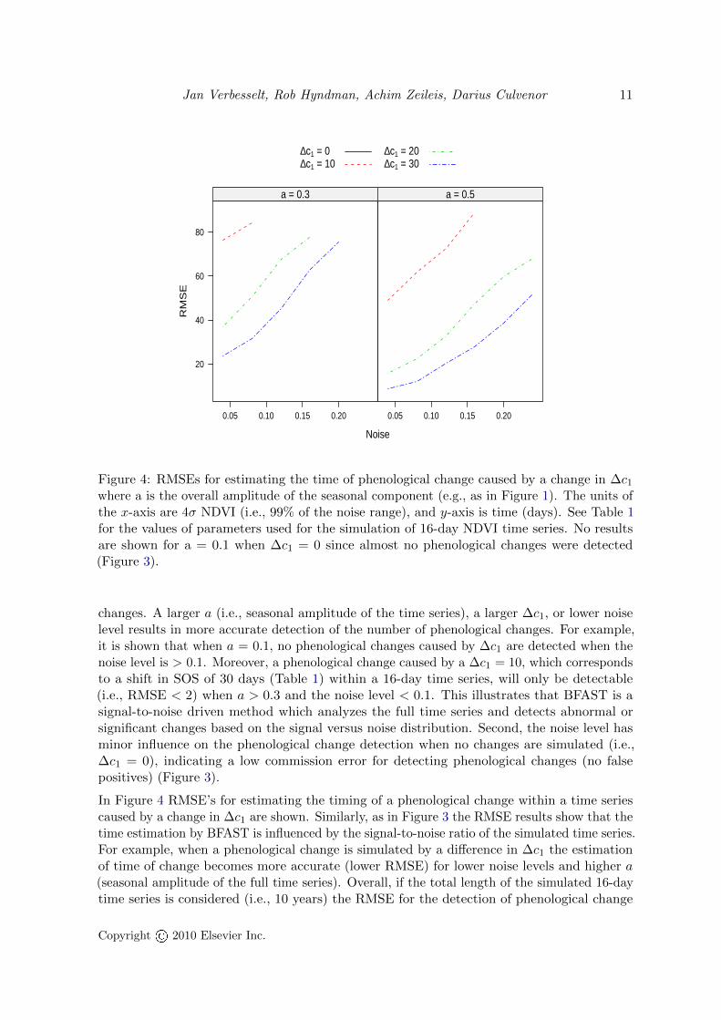
Figure 4: RMSEs for estimating the time of phenological change caused by a change in ∆c1where a is the overall amplitude of the seasonal component (e.g., as in Figure 1). The units ofthe x-axis are 4σ NDVI (i.e., 99% of the noise range), and y-axis is time (days). See Table 1for the values of parameters used for the simulation of 16-day NDVI time series. No resultsare shown for a = 0.1 when ∆c1 = 0 since almost no phenological changes were detected(Figure 3).

changes. A larger a (i.e., seasonal amplitude of the time series), a larger ∆c1, or lower noiselevel results in more accurate detection of the number of phenological changes. For example,it is shown that when a = 0.1, no phenological changes caused by ∆c1 are detected when thenoise level is > 0.1. Moreover, a phenological change caused by a ∆c1 = 10, which correspondsto a shift in SOS of 30 days (Table 1) within a 16-day time series, will only be detectable(i.e., RMSE < 2) when a > 0.3 and the noise level < 0.1. This illustrates that BFAST is asignal-to-noise driven method which analyzes the full time series and detects abnormal orsignificant changes based on the signal versus noise distribution. Second, the noise level hasminor influence on the phenological change detection when no changes are simulated (i.e.,∆c1 = 0), indicating a low commission error for detecting phenological changes (no falsepositives) (Figure 3).

In Figure 4 RMSE’s for estimating the timing of a phenological change within a time seriescaused by a change in ∆c1 are shown. Similarly, as in Figure 3 the RMSE results show that thetime estimation by BFAST is influenced by the signal-to-noise ratio of the simulated time series.For example, when a phenological change is simulated by a difference in ∆c1 the estimationof time of change becomes more accurate (lower RMSE) for lower noise levels and higher a(seasonal amplitude of the full time series). Overall, if the total length of the simulated 16-daytime series is considered (i.e., 10 years) the RMSE for the detection of phenological change



caused by a change in ∆c1 within a full time series remains low (i.e., < 3% of the length ofthe time series) for time series with a noise level < 0.15 and a seasonal amplitude a > 0.1.

4.2. Detecting phenological change in real MODIS image time series

Time of major phenological changes detected within 16-day NDVI image time series in astudy area containing a P. radiata plantation surrounded by grasslands are shown in Figure 5.Almost no phenological changes are detected in the forest plantations whereas phenologicalchanges are nearly always detected in the grasslands surrounding the forest plantation. Theseresults confirm the simulation results by showing that the detection of phenological changeswithin time series is influenced by the signal-to-noise ratio of the time series. The overallseasonal amplitude of a NDVI time series is larger for a grassland than for an evergreen forest(i.e., plantation) whereas the noise levels within NDVI time series are similar.

Figures 6 and 7 are examples of detected phenological and trend changes within a NDVItime series (2000–2009) extracted from a single MODIS pixel within a grassland and a forestcompartment located in the study area. Two phenological changes are detected in the seasonalcomponent of a grassland NDVI time series (Figure 6) whereas no phenological changes are

0 2 km

2002

2003

2004

2005

2006

2007

2008

Figure 5: Timing of long term phenological changes detected in MODIS NDVI image timeseries (2000–2009) for a forested area in south eastern Australia. The minimum period betweenbreaks is two years, which means that detected change is occurring over a period of two yearsor longer (see 2.2). The black line indicates the boundary of the Pinus radiata plantation,which corresponds to the area (white = no change) where less changes are detected. Theplantation is surrounded by grasslands.



0.2

0.5

0.8

da

ta

−0

.30

.00

.3

se

aso

na

l

0.2

0.5

0.8

tre

nd

−0

.20

.00

.2

2000 2002 2004 2006 2008 2010

rem

ain

de

r

Time

Figure 6: Detected changes in the seasonal and trend component (red) of 16-day NDVI timeseries (data) extracted from a single MODIS pixel of a grassland (Lat. 35.4◦ S, Lon. 147.9 ◦ E).The estimated average seasonal amplitude of the seasonal component is 0.7, with ∆a of -0.1for the seasonal change detected in 2006. Three abrupt changes are detected in the trendcomponent. The time of change (- - -), together with its confidence intervals (red) are alsoshown.

detected in NDVI time series of a P. radiata plantation (Figure 7). The figures illustrate thedifference in signal-to-noise ratio for a grassland versus a forest NDVI time series. The mostsignificant difference between a grassland and a forest NDVI time series is the data range ofthe seasonal component of 0.6 and 0.04, respectively. Figure 7 illustrates that the detection ofphenological changes in time series with a small signal-to-noise ratio (e.g., seasonal amplitude< 0.1 NDVI versus a noise level of approximately > 0.1 NDVI) is not possible. These resultsconfirm the simulation results by showing that the detection of phenological changes withintime series is influenced by the signal-to-noise ratio of the time series.

Figure 5 illustrates that the major phenological changes detected in the grasslands occur inbetween 2005 and 2006. While the study area was experiencing below average annual rainfallsince 2001, a major rainfall anomaly occurred in the study area from 2006 onwards causingsevere drought stress (Figure 8). Figure 6 illustrates a phenological change detected in 2006with a seasonal segment (2006–2010) that has a smaller amplitude and a later start of thegrowing season compared to the other seasonal segments (i.e., 2000–2002 and 2002–2006)resulting from the piecewise robust linear regression. The trend component of Figures 6 and 7also shows an abrupt change occurring in 2007 and a gradual decline (negative slope) fromthen onwards which confirms that the drought stress has a negative long term impact on theseasonal growth cycle. The occurrence of abrupt and gradual changes in the trend componentin the study are further discussed in detail by Verbesselt et al. (2010).



0.7

50

.85

da

ta

−0

.02

0.0

1

se

aso

na

l

0.7

50

.85

tre

nd

−0

.06

0.0

0

2000 2002 2004 2006 2008 2010

rem

ain

de

r

Time

Figure 7: Detected changes in trend component (red) of 16-day NDVI time series (data)extracted from a single MODIS pixel of a Pinus radiata plantation (Lat. 35.5◦ S, Lon. 148.0◦ E)with plant year 1974. The estimated average seasonal amplitude of the seasonal component is0.1, with three abrupt changes detected in the trend component and no phenological changesdetected in the seasonal component. The time of change (- - -), together with its confidenceintervals (red) are also shown.

2000 2001 2002 2003 2004 2005 2006 2007 2008 20090

200

400

600

800

1000

1200

Figure 8: Annual rainfall (mm/year) for North Western part of Green Hills State Forest wherethe (—) line illustrates the mean annual rainfall, 1072mm/year between 1940–2009 derivedfrom interpolated rainfall surfaces with a spatial resolution of 500 m (Jeffrey et al. 2001).



5. Discussion

The detection of phenological change within seasonal time series containing noise, phenological,abrupt and gradual changes is discussed:

(1) BFAST can be used to detect significant long term phenological changes by exploiting thefull time series while accounting for abrupt and gradual changes. Understanding of whatconstitutes significant change in land surface phenology (LSP) amidst background variationis a critical component of global change research (de Beurs and Henebry 2005a). Exploitingthe full time series enables the description of the continual process of LSP development,not just dates of specific events. Unlike in traditional ground-based phenology research inwhich dates may be recorded (e.g., flowering), LSP is the integral of multiple coincidentgrowth cycles, non-climatic factors, and data quality (de Beurs and Henebry 2004; Whiteand Nemani 2006). Furthermore, the high interannual variability of phenological metricsdemonstrates the necessity of distinguishing annual seasonal variability from long termphenological change (Bradley and Mustard 2008). In this study a long term phenologicalchange is defined relative to the total length of the studied NDVI time series (i.e., 10years) as a significant phenological change occurring over a period longer than two years.Long term phenological change within satellite image time series is a relative conceptwhen compared to global change analysis dealing with in-situ phenology or climate datatime series of 100 years and longer (Schwartz 1999). Methods able to exploit full timeseries and detect long term changes will become more important in the context of everincreasing length of satellite image time series.

(2) Results illustrate that the capacity of BFAST to detect changes within time series isinfluenced by the signal-to-noise ratio of the time series. A wide range of NDVI specificnoise levels representative for MODIS time series were simulated and used to assessBFAST’s robustness against noise (Verbesselt et al. 2010). Results showed that BFASThas a low commission error for different noise levels when no phenological changes weresimulated (no false positives). BFAST deals with noise in time series in two ways. First,robust linear regression is implemented to reduce the influence of outliers (e.g., clouds)(Venables and Ripley 2002) when iteratively estimating the seasonal and trend model.Secondly, three harmonic terms are used to estimate the seasonal component of a timeseries and remove higher frequency variations such as noise and atmospheric scatter(Geerken 2009).

Furthermore, it was shown that the detection of phenological change was influenced bythe signal-to-noise ratio of the time series (i.e., seasonal amplitude versus noise). Thelower the noise level and the larger the seasonal amplitude or phenological change withinthe time series, the easier it is to detect a phenological change within a time series.This confirms the importance of other available techniques to improve the signal-to-noiseratio of a time series. Elimination of noise within satellite image time series requiresattention to issues of satellite calibration, orbital correction, detection and removal ofatmospheric contamination, and image registration. Compositing of time series aimsat lowering atmospheric and cloud influence (Holben 1986), with different compositingperiods ranging usually from 8 to 16 days. Compositing of time series and advanced cloudmasking techniques do not fully eliminate effects of clouds and atmospheric contamination.Application of methods that estimate the upper envelope of the NDVI time series further



reduce the influence of cloud contaminated values and improve the signal-to-noise ratioof a NDVI time series (Julien and Sobrino 2010; Roerink, Menenti, and Verhoef 2000;Viovy, Arino, and Belward 1992). In summary, BFAST deals with inherent noise in timeseries but the application of other available techniques which improve data quality remainsimportant.

(3) It is shown that the seasonal amplitude of time series impacts the signal noise ratio anddetermines the capacity to detect phenological changes. Phenological changes can notbe detected in seasonal time series having a signal-to-noise ratio smaller than one (e.g.,having a seasonal amplitude ≤ 0.1 and a noise range ≥ 0.1 NDVI). Application of BFASTon real MODIS satellite image time series showed that more phenological changes weredetected within grasslands than in P. radiata plantations. The seasonal amplitude ofgrasslands (i.e., > 0.3 NDVI) is significantly larger than for evergreen plantations (i.e.,< 0.1 NDVI). The simulation analysis supports these findings by illustrating that thedetection of phenological change within time series is influenced by the signal-to-noiseratio. Moreover, simulation results also illustrated that phenological changes can stillbe detected within NDVI time series of the majority of the global land cover types, e.g.,grasslands, woodlands, deciduous or open forests, having a larger signal-to-noise ratio(> 1). These findings corroborate results of Julien and Sobrino (2009) and de Beurs et al.(2009) by excluding time series exhibiting low seasonal amplitude from the phenologicaltrend analysis. Julien and Sobrino (2009) did not analyze phenology trends in NDVI timeseries of biomes with a amplitude smaller than 0.1 that were extracted from the globalGIMMS NDVI data set (1981–2003). These biomes correspond to arid or frozen area,as well as evergreen dense vegetation (Julien and Sobrino 2009). Also, de Beurs et al.(2009) excluded MODIS NDVI time series from the analysis with a coefficient of variation< 5% to ensure sufficient seasonality to produce reliable trend estimates of extractedphenological metrics. Furthermore, the detection of phenological change in evergreenforests is difficult with remotely sensed NDVI time series since the NDVI tends to saturatefor high biomass regions such as evergreen forests (Huete et al. 2002). Other more sensitiveremotely sensed indices for high biomass regions such as the Enhanced Vegetation index(Huete et al. 2002) or SWIR-based indices (Hunt and Rock 1989; de Beurs and Townsend2008) may produce better results.

6. Further work and applications

(1) The BFAST algorithm can potentially be used for studies of vegetation dynamics andphenology in two ways (Figure 9). First, as illustrated in this study BFAST can be usedto detect long term phenological changes within time series by analyzing the seasonalcomponent of the time series for changes in phenology (Figure 9, St). Phenologicalchanges are detected independent of the change type since a harmonic model is used thataccommodates for a large range of land cover types (Jakubauskas, Legates, and Kastens2001). The detected phenological changes can be characterized by the fitted parameters ofthe harmonic model (i.e., aj and δj). Second, underlying trend can be removed from timeseries to improve the data quality (Figure 9, Yt − Tt). For example, satellite sensor errorshave a longer term impact on the signal (e.g., sensor drift and calibration problems) and



Remotely sensed time series

BFAST

Figure 9: A flow chart illustrating how BFAST can be used for phenology studies. Yt is asimulated 16-day NDVI time series used as an input (Figure 2). First, the method can be usedto detect phenological change within time series (left). Two phenological changes are detectedin the seasonal component (St). Second, time series can be corrected for underlying trendsby accounting for abrupt and gradual changes (right). One abrupt change and a gradualrecovery is shown in the trend component (Tt) and used to obtain the trend corrected timeseries, Yt − Tt.

will affect the underlying trend in long time series (Bradley and Mustard 2008). As such,by removing the underlying trends from the original time series to correct for satellitesensor errors having an impact on the signal. Available methods to extract phenologicalmetrics can be applied on these trend corrected time series.

(2) The utility of the time series simulation approach proposed in this study provides theability to test phenological change detection methods in a controlled environment. Whilevalidation is a key issue in remotely sensed phenology studies over large areas (Reed et al.2003; Schwartz, Reed, and White 2002; White et al. 2009), field data defining full seasonalgrowth cycles over multiple years is lacking. Traditional ground-based phenology researchhas been focussing on recording specific dates (e.g., flowering or budburst) (Schwartz 1999)whereas satellite sensors record daily information about LSP requiring a similar type of



temporally continuous field data to be collected. This explains why relationships betweenremotely sensed LSP and plant phenology are generally unknown (White and Nemani2006). The simulation of time series approach enables the assessment of methods to studyphenological changes in a controlled environment by varying the signal-to-noise ratio andcombining it with simulated changes within time series.

(3) The parametric seasonal and trend models used within BFAST provide a natural frameworkfor real time monitoring and forecasting. White and Nemani (2006) proposed a conceptualapproach to real time monitoring and short term forecasting of LSP. Although White andNemani (2006) state that phenology information should not be provided for individualpixels (individual time series) there are some corresponding principles. First, BFAST alsoavoids defining phenological metrics and detects phenological change based on a significantdifference between phenological models by employing a piecewise robust linear regression.Second, the estimated models in BFAST can not only be assessed using historical data todetect changes; but given the detected changes, short term forecasts from the last stablemodel can be derived (Pesaran and Timmermann 2002). The deviations between theseforecasts and the incoming observations can be utilized for monitoring the stability of themodel in real time (Zeileis 2005). Further work is required to evaluate and demonstrateBFAST for real monitoring and forecasting.

7. Conclusion

A challenge to phenology studies is understanding what constitutes long term phenologicalchange amidst background variation (e.g., fires, land degradation, and noise). Here, wedemonstrated the ability of a method to detect long term phenological change by analyzingtime series containing noise, abrupt, and gradual changes. Exploiting full time series enablesthe description of the continual process of land surface phenology, not just dates of specificevents. The method, BFAST (Breaks For Additive Seasonal and Trend), iteratively estimatesthe dates and number of changes occurring within seasonal and trend components (Verbesseltet al. 2010). The method has been improved by implementing a harmonic seasonal modelwhich requires fewer observations, is more robust against noise, and of which the parameterscan be more easily used to characterize phenological change.

We tested BFAST (1) by simulating 16-day NDVI time series with varying seasonal amplitudeand noise, containing an abrupt trend change and long term phenological changes, and (2)by applying on MODIS NDVI time series covering a forested area in south eastern Australia.Results showed that the number and timing of detected phenological changes within timeseries is influenced by the signal-to-noise ratio of the analyzed time series. BFAST dealswith inherent noise in time series using robust linear regression techniques and using only thefirst three harmonic terms for the seasonal model estimation. However, it remains importantto improve the data quality of time series by using existing techniques to reduce the noiselevel and increase the signal-to-noise ratio. It is shown that the seasonal amplitude of NDVItime series impacts the signal-to-noise ratio and determines the ability to detect phenologicalchanges. Phenological changes caused by a change in SOS can not be detected in seasonaltime series having a signal-to-noise ratio smaller than one (i.e., having a seasonal amplitude≤ 0.1 NDVI and a noise range ≥ 0.1 NDVI). Other more sensitive remotely sensed indicesfor high biomass regions (i.e., evergreen forests) may improve the detection of phenological



changes by increasing the measured seasonal amplitude. However, phenological changes canstill be detected within NDVI time series of the majority of the global land cover types, e.g.,grasslands, woodlands, deciduous or open forests, having a signal-to-noise ratio > 1.

The proposed method can be used in two ways for phenology studies. First, as demonstratedhere it can be used to detect long term phenological changes within time series. Second, itcan be used to remove underlying abrupt and gradual trend changes and improve the qualityof time series data before for example extraction of phenological metrics. BFAST can beapplied to any time series data and it is not limited to NDVI. The method described in thisstudy are available in the bfast package for R (R Development Core Team 2009) from CRAN(http://CRAN.R-project.org/package=bfast).

Acknowledgements

This work was undertaken within the program of the Cooperative Research Center for Forestry:Monitoring and Measuring (http://www.crcforestry.com.au/). Thanks to Dr. GlennNewnham and Dr. Michael Dunlop whose comments greatly improved this paper. We greatlyappreciate the constructive feedback we have received from the three reviewers.

References

Anyamba A, Eastman JR (1996). “Interannual variability of NDVI over Africa and itsrelation to El Nino Southern Oscillation.” International Journal of Remote Sensing, 17(13),2533–2548.

Azzali S, Menenti M (2000). “Mapping vegetation-soil-climate complexes in southern Africausing temporal Fourier analysis of NOAA-AVHRR NDVI data.” International Journal ofRemote Sensing, 21(5), 973–996.

Bai J, Perron P (2003). “Computation and analysis of multiple structural change models.”Journal of Applied Econometrics, 18(1), 1–22.

Bontemps S, Bogaert P, Titeux N, Defourny P (2008). “An object-based change detectionmethod accounting for temporal dependences in time series with medium to coarse spatialresolution.” Remote Sensing of Environment, 112(6), 3181–3191.

Bradley BA, Jacob RW, Hermance JF, Mustard JF (2007). “A curve fitting procedure toderive inter-annual phenologies from time series of noisy satellite NDVI data.” RemoteSensing of Environment, 106(2), 137–145.

Bradley BA, Mustard JF (2008). “Comparison of phenology trends by land cover class: a casestudy in the Great Basin, USA.” Global Change Biology, 14(2), 334–346.

Cleland EE, Chuine I, Menzel A, Mooney HA, Schwartz MD (2007). “Shifting plant phenologyin response to global change.” Trends in Ecology & Evolution, 22(7), 357–365.

Coppin P, Jonckheere I, Nackaerts K, Muys B, Lambin E (2004). “Digital change detectionmethods in ecosystem monitoring: a review.” International Journal of Remote Sensing,25(9), 1565–1596.


http://CRAN.R-project.org/package=bfast

http://www.crcforestry.com.au/


Crist EP, Cicone RC (1984). “A physically-based transformation of thematic mapper data– The TM Tasseled cap.” IEEE Transactions on Geoscience and Remote Sensing, 22(3),256–263.

de Beurs K, Wright C, Henebry G (2009). “Dual scale trend analysis for evaluating cli-matic and anthropogenic effects on the vegetated land surface in Russia and Kazakhstan.”Environmental Research Letters, 4(4).

de Beurs KM, Henebry GM (2004). “Trend analysis of the Pathfinder AVHRR Land (PAL)NDVI data for the deserts of central Asia.” Geoscience and Remote Sensing Letters, IEEE,1(4), 282–286. ISSN 1545-598X.

de Beurs KM, Henebry GM (2005a). “Land surface phenology and temperature variation inthe International Geosphere-Biosphere Program high-latitude transects.” Global ChangeBiology, 11(5), 779–790.

de Beurs KM, Henebry GM (2005b). “A statistical framework for the analysis of long imagetime series.” International Journal of Remote Sensing, 26(8), 1551–1573.

de Beurs KM, Townsend PA (2008). “Estimating the effect of gypsy moth defoliation usingMODIS.” Remote Sensing of Environment, 112(10), 3983–3990.

Eastman JR, Sangermano F, Ghimire B, Zhu H, Chen H, Neeti N, Cai Y, Machado EA, CremaSC (2009). “Seasonal trend analysis of image time series.” International Journal of RemoteSensing, 30(10), 2721–2726.

Fensholt R, Rasmussen K, Nielsen TT, Mbow C (2009). “Evaluation of earth observation basedlong term vegetation trends – Intercomparing NDVI time series trend analysis consistencyof Sahel from AVHRR GIMMS, Terra MODIS and SPOT VGT data.” Remote Sensing ofEnvironment, 113(9), 1886 – 1898.

Geerken RA (2009). “An algorithm to classify and monitor seasonal variations in vegetationphenologies and their inter-annual change.” ISPRS Journal of Photogrammetry and RemoteSensing, 64(4), 422–431.

Holben BN (1986). “Characteristics of maximum-value composite images from temporalAVHRR data.” International Journal of Remote Sensing, 7(11), 1417–1434.

Huete A, Didan K, Miura T, Rodriguez EP, Gao X, Ferreira LG (2002). “Overview of theradiometric and biophysical performance of the MODIS vegetation indices.” Remote Sensingof Environment, 83(1-2), 195–213.

Hunt ER, Rock BN (1989). “Detection of change in leaf water-content using near-infrared andmiddle-infrared reflectances.” Remote Sensing of Environment, 30(1), 43–54.

Jakubauskas ME, Legates DR, Kastens JH (2001). “Harmonic analysis of time-series AVHRRNDVI data.” Photogrammetric Engineering and Remote Sensing, 67(4), 461–470.

Jeffrey SJ, Carter JO, Moodie KB, Beswick AR (2001). “Using spatial interpolation toconstruct a comprehensive archive of Australian climate data.” Environmental Modelling &Software, 16(4), 309–330.



Julien Y, Sobrino JA (2009). “Global land surface phenology trends from GIMMS database.”International Journal of Remote Sensing, 30(13), 3495–3513.

Julien Y, Sobrino JA (2010). “Comparison of cloud-reconstruction methods for time series ofcomposite NDVI data.” Remote Sensing of Environment, 114(3), 618–625.

Lambin EF, Strahler AH (1994). “Change-Vector Analysis in multitemporal space - A ToolTo Detect And Categorize Land-Cover Change Processes Using High Temporal-ResolutionSatellite Data.” Remote Sensing of Environment, 48(2), 231–244.

Linderholm HW (2006). “Growing season changes in the last century.” Agricultural and ForestMeteorology, 137(1-2), 1–14.

Makridakis S, Wheelwright SC, Hyndman RJ (1998). Forecasting: methods and applications.3rd edition. John Wiley & Sons, New York.

Parmesan C, Yohe G (2003). “A globally coherent fingerprint of climate change impacts acrossnatural systems.” Nature, 421(6918), 37–42.

Pesaran MH, Timmermann A (2002). “Market Timing and Return Prediction Under ModelInstability.” Journal of Empirical Finance, 9, 495–510.

Potter C, Tan PN, Steinbach M, Klooster S, Kumar V, Myneni R, Genovese V (2003). “Majordisturbance events in terrestrial ecosystems detected using global satellite data sets.” GlobalChange Biology, 9(7), 1005–1021.

R Development Core Team (2009). R: A Language and Environment for Statistical Computing. RFoundation for Statistical Computing, Vienna, Austria. URL http://www.R-project.org/.

Reed BC, White M, Brown JF (2003). “Remote sensing phenology.” Phenology: an IntegrativeEnvironmental Science, 39, 365–381.

Roerink G, Menenti M, Verhoef W (2000). “Reconstructing cloudfree NDVI composites usingFourier analysis of time series.” International Journal of Remote Sensing, 21(9), 1911–1917.

Schwartz MD (1999). “Advancing to full bloom: planning phenological research for the 21stcentury.” International Journal of Biometeorology, 42(3), 113–118.

Schwartz MD, Reed BC, White MA (2002). “Assessing satellite-derived start-of-season measuresin the conterminous USA.” International Journal of Climatology, 22(14), 1793–1805.

Townshend JRG, Justice CO (1988). “Selecting the spatial-resolution of satellite sensorsrequired for global monitoring of land transformations.” International Journal of RemoteSensing, 9(2), 187–236.

Venables WN, Ripley BD (2002). Modern applied statistics with S. 4th edition. Springer-Verlag.

Verbesselt J, Hyndman R, Newnham G, Culvenor D (2010). “Detecting trend and seasonalchanges in satellite image time series.” Remote Sensing of Environment, 114(1), 106–115.

Verbesselt J, Jonsson P, Lhermitte S, van Aardt J, Coppin P (2006). “Evaluating satelliteand climate data derived indices as fire risk indicators in savanna ecosystems.” IEEETransactions on Geoscience and Remote Sensing, 44(6), 1622–1632.


http://www.R-project.org/


Viovy N, Arino O, Belward AS (1992). “The Best Index Slope Extraction (BISE) - a methodfor reducing noise in NDVI time-series.” International Journal of Remote Sensing, 13(8),1585–1590.

Wagenseil H, Samimi C (2006). “Assessing spatio-temporal variations in plant phenology usingFourier analysis on NDVI time series: results from a dry savannah environment in Namibia.”International Journal of Remote Sensing, 27(16), 3455–3471.

White MA, de Beurs KM, Didan K, Inouye DW, Richardson AD, Jensen OP, O’Keefe J, ZhangG, Nemani RR, van Leeuwen WJD, Brown JF, de Wit A, Schaepman M, Lin X, DettingerM, Bailey AS, Kimball J, Schwartz MD, Baldocchi DD, Lee JT, Lauenroth WK (2009).“Intercomparison, interpretation, and assessment of spring phenology in North Americaestimated from remote sensing for 1982–2006.” Global Change Biology, 15, 2335–2359.

White MA, Nemani AR (2003). “Canopy duration has little influence on annual carbon storagein the deciduous broad leaf forest.” Global Change Biology, 9(7), 967–972.

White MA, Nemani RR (2006). “Real-time monitoring and short-term forecasting of landsurface phenology.” Remote Sensing of Environment, 104(1), 43–49.

White MA, Thornton PE, Running SW (1997). “A continental phenology model for monitoringvegetation responses to interannual climatic variability.” Global Biogeochemical Cycles,11(2), 217–234.

Zeileis A (2005). “A Unified Approach to Structural Change Tests Based on ML Scores, FStatistics, and OLS Residuals.” Econometric Reviews, 24(4), 445–466.

Zeileis A, Kleiber C (2005). “Validating multiple structural change models – A case study.”Journal of Applied Econometrics, 20(5), 685–690.

Zeileis A, Kleiber C, Kramer W, Hornik K (2003). “Testing and Dating of Structural Changesin Practice.” Computational Statistics and Data Analysis, 44, 109–123.

Zeileis A, Leisch F, Hornik K, Kleiber C (2002). “strucchange: An R Package for Testing forStructural Change in Linear Regression Models.” Journal of Statistical Software, 7(2), 1–38.URL http://www.jstatsoft.org/v07/i02/.

Zhang XY, Friedl MA, Schaaf CB, Strahler AH, Hodges JCF, Gao F, Reed BC, Huete A(2003). “Monitoring vegetation phenology using MODIS.” Remote Sensing of Environment,84(3), 471–475.

Affiliation:

Jan VerbesseltAustralian Commonwealth Scientific and Research OrganizationRemote Sensing TeamPrivate Bag 10, Melbourne VIC 3169, AustraliaE-mail: [email protected]


http://www.jstatsoft.org/v07/i02/

mailto:[email protected]

Date post:	01-Jan-2017
Category:	Documents
Upload:	doanhanh
View:	218 times
Download:	0 times

Phenological Change Detection while Accounting for Abrupt and ...

Documents