Physics-Based Low-Order Model for Transonic Flutter...

Physics-Based Low-Order Model

for Transonic Flutter Prediction

Max M. J. Opgenoord∗, Mark Drela†, and Karen E. Willcox‡

Massachusetts Institute of Technology, Cambridge, MA, 02139

This paper presents a physical low-order model for two-dimensional unsteady transonicairfoil flow, based on small unsteady disturbances about a known steady flow solution.This is in contrast to traditional small-disturbance theory which assumes small distur-bances about the freestream. The states of the low-order model are the flowfield’s lowestmoments of vorticity and volume-source density perturbations, and their evolution equa-tion coefficients are calibrated using off-line unsteady CFD simulations through dynamicmode decomposition. The resulting low-order unsteady flow model is coupled to a typical-section structural model, thus enabling prediction of transonic flutter onset for moderateto high aspect ratio wings. The method is fast enough to permit incorporation of tran-sonic flutter constraints in conceptual aircraft design calculations. The accuracy of thislow-order model is demonstrated for forced pitching and heaving simulations of an airfoilin compressible flow. Finally, the model is used to describe the influence of compressibilityon the flutter boundary, and its accuracy is demonstrated for the Isogai Case A classicalflutter test case.

Nomenclature

A, E State-space matricesAa, Ba State-space matrices of aerodynamic

systemAΓ, AΓ, Aκ Coefficients of Γ evolution equationBΓ, Bκ, Bκ Coefficients of κx evolution equationDwave Wave dragIθ Moment of inertia around elastic axisL LiftMcrit Critical Mach numberM∞ Free stream Mach numberSθ Mass unbalanceV Velocity fieldV0 Velocity field of steady solutionVµ Flutter speed indexV∞ Free stream velocityX, X ′, X ′′ Matrices containing sequences of

snapshots of state vectora Local speed of sounda, al, b Discrete state-space matricesc Airfoil chord lengthc` Lift coefficientd Distance between quarter-chord and

elastic axish Vertical position, positive downward

kh Spring constant for vertical motionkθ Torsional spring constantm Massn Normal unit vectorr Position vectorrθ Radius of gyration about the airfoil’s

elastic axist Timeu State-space control vectorua State-space control vector of aerody-

namic systemw Vertical velocity, positive downwardx State-space vectorx, z Physical coordinates along freestreamxa State-space vector of aerodynamic

systemxcg Position of center of gravity relative to

leading edgexea Position of elastic axis relative to lead-

ing edge

Symbols

α Angle of attackΓ Circulation strength

∗Graduate student, Department of Aeronautics and Astronautics, [email protected], Student Member AIAA†Terry J. Kohler Professor of Aeronautics and Astronautics, Department of Aeronautics and Astronautics, [email protected],

Fellow AIAA‡Professor of Aeronautics and Astronautics, [email protected], Associate Fellow AIAA

1 of 20

American Institute of Aeronautics and Astronautics

θ Pitch angleκx x-doublet strengthµ Apparent mass ratioρ∞ Free stream densityσ Volume-source strengthΥ′ Matrix containing sequence of snap-

shots of control input vector

φ Velocity potentialω Vorticityω Angular velocityω Reduced frequencyωθ, ωh Uncoupled in-vacuo natural frequen-

cies in pitch and heave

I. Introduction

The push for more efficient transport aircraft leads to larger wing spans and more flexible wings, config-urations for which flutter becomes a significant design consideration. This is especially true for next-

generation airplane concepts, such as the Truss-Braced Wing.1 However, incorporating flutter prediction intoearly-stage design is a considerable challenge for the transonic flow regime relevant to most civil transportaircraft designs, since existing accurate models for transonic flutter prediction typically require extensivecomputational fluid dynamic (CFD) analyses that are too expensive to conduct in early design stages wherepotentially thousands of wing designs might be considered. Flutter constraints can be included in state-of-the-art multidisciplinary design optimization settings, but even if the static aeroelastic methods are highfidelity, the methods for unsteady (compressible) flow usually either linearize the unsteady response or usea Prandtl-Glauert correction,2,3 which is limited to subsonic flow. In this paper, we develop an accurate,fast, low-order model for small-amplitude transonic unsteady airloads, intended for flutter prediction inearly-stage design and optimization of transport aircraft.

While flutter for low subsonic flows can, in general, be accurately predicted with linearized small-disturbance theories, they fail for transonic flow where the traditional small-disturbance formulation isinherently nonlinear.4 For example, linear theory predicts that thinner wings would be less susceptible toflutter, but wind tunnel tests have shown the opposite to be true.4 Another interesting phenomenon thatoccurs in transonic flows is the transonic dip in the flutter boundary.5–8 Linear theories cannot predict thelocation or shape of the transonic dip, and tend to produce optimistic estimates for the flutter boundary.9

The seminal work by Theodorsen10 is widely used for incompressible flutter predictions for two-dimensionalairfoils. Several researchers extended Theodorsen’s theory to subsonic flows,11–13 with none of these methodsextending to the transonic regime. Moreover, Theodorsen theory is only strictly valid for simple harmonicmotion, which strictly applies only at the flutter boundary.

Possio14 applied the acceleration potential to a two-dimensional subsonic compressible nonstationaryproblem and arrived at an integral equation (Possio’s equation) for subsonic unsteady compressible flow.Closed-form solutions to an approximation of Possio’s equation were found in 1999.15,16 However, theaccuracy for Possio’s method deteriorates for transonic flows and for high-frequency oscillations.17 Lomax etal.18 used piston theory to analytically find the lift response to unsteady perturbations in subsonic flow, butonly for the non-circulatory part of the lift. Stahara and Spreiter,19 Isogai,20 and Dowell21 developed modelsfor linearized transonic flow, applicable to thin airfoils in shock-free flows. A linearization of the TransonicSmall-Disturbance (TSD) equation for unsteady transonic flow was first proposed by Nixon,22 which involveschanging the airfoil geometry for transonic flows such that the shock location does not change during anyperturbations.

These analytical/theoretical methods all suffer from a loss of accuracy in transonic flows with shockson the airfoil surface, which are typical on jet transports. Other approaches have attempted to addressthis limitation by deriving models using a combination of theory and experimental data, as in the workof Leishman and Nguyen23 who formulated a state-space representation of unsteady airfoil behavior withsome parameters estimated from experimental data, or by deriving reduced-order models from high-fidelityCFD models. A reduced-order modeling approach starts with the full state (flow field) information collectedfrom a CFD solver and identifies a low-dimensional subspace in which the most important system dynamicsevolve.24 Methods such as the harmonic balance,25 proper orthogonal decomposition,26–28 and Volterraseries29 have all been used to derive aeroelastic reduced-order models.30 These methods have been appliedin practice successfully, amongst others, for unsteady transonic flow around full wings,31 a full F-16 aircraftconfiguration,32 and many more.

In contrast to the reduced-order modeling approach, which starts with a high-order model and reducesthe state by pure numerics, our work constructs a physics-based low-order model a priori, in terms of

2 of 20


the flowfield’s volume-source and vorticity moments. Our state variables are the unsteady perturbationsof these moments from some known steady transonic solution, and their time evolution is governed bypostulated equations whose coefficients are treated as parameters. These parameters are calibrated usinghigh-fidelity CFD results. Our underlying assumption is that the baseline steady flow is statically nonlinear,but sufficiently small disturbances around the baseline solution can be assumed to produce a linear responsein the overall volume-source and vorticity moments.33 The resulting model produces unsteady perturbationlift and moment outputs, which can be combined with a conventional typical-section structural elastic modelto obtain an overall aeroelastic state-space model suitable for flutter prediction.

We develop the present aerodynamic model as an extension of the one used in ASWING,34,35 whichemploys Theodorsen theory10 for calibration. In contrast, the present model is calibrated using data fromhigh-fidelity Euler CFD simulations of the transonic unsteady flow around airfoils. Section II of this paperdevelops the physics-based low-order model. Section III describes the state-space system identificationmethods used to fit the model coefficients using CFD data. Section IV demonstrates the model’s ability topredict transonic flutter, and Section V concludes the paper.

II. Physics-Based State-Space Model Formulation

This section develops the physics-based low-order model. We start with the aerodynamic low-order model,of which some coefficients will have to be calibrated—the calibration is discussed in Section III—and thenmove on to the structural model. The aerodynamic and structural models are combined in an aeroelasticstate-space system. Analysis of the coupled state-space system indicates whether flutter occurs.

II.A. Aerodynamic Low-Order Model

The physics-based low-order aerodynamic model begins with the Helmholtz decomposition, which expressesany instantaneous velocity field V as integrals over the velocity’s divergence and curl fields, commonly knownas the volume-source density σ and the vorticity ω:

σ ≡ ∇ ·V (1)

ω ≡ ∇×V (2)

V(r, t) =1

2π

∫∫σ(r′, t)

r−r′

|r−r′|2dA′ +

1

2π

∫∫ω(r′, t)× r−r′

|r−r′|2dA′ + V∞, (3)

where r is a position vector, t is time, and V∞ is the free-stream velocity field. For low-speed flow we haveσ = 0 by mass continuity, and for potential flow the ω field is restricted to the body boundary layers andwakes where it can be approximated via vortex filaments or the equivalent normal-doublet panels. This is thebasis of vortex-lattice or doublet-lattice methods. For compressible flows the volume-source field σ becomessignificant due to density gradients, but for small-disturbance subsonic flows it can be linearized and removedvia the Prandtl-Glauert transformation.36 Although this linearization approach fails for transonic flows, thevelocity decomposition (3) is a mathematical identity and always remains valid, provided the volume-sourcefield σ is defined and computed appropriately. One example is given by Oskam,37 who obtained 2D transonicairfoil solutions using this approach. Specifically, the volume-source field was represented by panels coveringspace around the airfoil, whose σ strengths were computed via the full-potential equation, together with theusual normal-doublet panels on the surface computed via flow tangency.

We define the unsteady volume-source and vorticity fields to have the form

σ(r, t) = σ0(r) + ∆σ(r, t) (4)

ω(r, t) = ω0(r) + ∆ω(r, t), (5)

where σ0 and ω0 correspond to some known steady transonic flow, and ∆σ and ∆ω are small perturbationsdefining the unsteady flow we are seeking. Since the Helmholtz decomposition (3) is linear in σ and ω, thecorresponding velocity field will have the same baseline plus perturbation form:

V (r, t) = V0 (r) + ∆V (r, t) . (6)

We stress that “small disturbance” here refers to small disturbances from the steady solution, and not smallperturbations from the freestream (which is the more common usage).

3 of 20


To construct the low-order model for the overall airfoil lift and pitching moment, we first assume that theeffects of the σ and ω fields, diagrammed in Figure 1, can be captured by only their leading spatial moments.The zeroth moment of the vorticity, or equivalently its overall lumped strength, is the airfoil circulation

Γ ≡∫∫

ω · y dA, (7)

where y is the unit vector into the plane. For steady flow, the circulation captures the lift exactly via theKutta-Joukowsky theorem. As sketched in Figure 1, the volume-source field σ is mostly positive over theupper front of the airfoil where the flow accelerates, and mostly negative over the shock and the upper rearwhere the flow decelerates. Its zeroth moment is comparable to the wave drag, which typically is very smalland negligible compared to the lift force:

Dwave

ρ∞V∞'∫∫

σ dA ' 0. (8)

Consequently, we must consider the first x-moment of the volume-source field, which is its overall lumpedx-doublet strength,

κx(t) ≡∫∫−xσ dA. (9)

In the single-element Weissinger vortex-lattice method,38,39 all the vorticity is lumped into a point vortexplaced at the airfoil quarter-chord point, and its strength Γ is implicitly determined by requiring the flow-tangency condition Vc.p. · nc.p. = 0 at the control point at the airfoil three-quarter chord point. For unsteadyflow there will be additional contributions from the shed vorticity that modify Vc.p. and hence Γ(t) and thelift, and also from the airfoil motion. This is the approach used in the ASWING formulation,34,35 which forlow-speed flow closely matches the results of the more exact Theodorsen theory.10

For the transonic flows considered here, this model is extended by the addition of the lumped x-doubletplaced at some location (xκ, zκ). As diagrammed in Figure 1, the doublet adds to the overall velocity at thecontrol point, and thus will affect Γ and the lift. This is the mechanism which is here postulated to capturethe compressibility effects on the circulation and the resulting lift and moment.

+

−

−

+

− +

( )σρ

r

∆

V,t

xκ

Γ

n

Vωω( )r,t −−−

∆

V

x

z

V

V

∆

ρρ

t+( )1

−−− = −

Figure 1. Vorticity and field sources representing velocity field are approximated by overall circulationΓ and doublet κx. Only their small unsteady perturbations from a transonic flowfield, ∆Γ and ∆κx,are sought in the present analysis.

Corresponding to decompositions (4) and (5), we will here actually seek the small perturbations

∆Γ(t) ≡ Γ(t)− Γ0 (10)

∆κx(t) ≡ κx(t)− κx,0 (11)

from the steady-solution values Γ0, κx,0. The steady circulation Γ0 is directly proportional to the steady liftcoefficient c`0 or the corresponding angle of attack α0, while κx,0 is also a strong function of the freestreamMach number M∞ and to some extent of the airfoil shape. Typical κx,0 variation for a transonic airfoil isshown in Figure 2. Note that the dependence on c`0 is almost linear.

4 of 20


cℓ0

0.35 0.4 0.45 0.5 0.55 0.6 0.65 0.7 0.75 0.8 0.85

κx,0/V∞c2

0

0.05

0.1

0.15

0.2

0.25

0.3

Fig. 5(b)

Fig. 5(a)

M = 0.75M = 0.70M = 0.65M = 0.60M = 0.55M = 0.50M = 0.45M = 0.40

Figure 2. Variation of κx,0 with c`,0 and Mach number for the RAE2822 transonic airfoil, as computedusing MSES.40–42

For the imposition of flow tangency at the control point, we define the instantaneous airfoil-surface normalvelocity at the control point as

Un(t) ≡ Uc.p. · nc.p., (12)

while the instantaneous fluid normal velocity at the control point is defined as

Vn(t) ≡ Vc.p. · nc.p.. (13)

Next, we approximate the normal fluid velocity perturbation at the three-quarter control point as

∆Vn(t) = AΓ∆Γ +AΓ∆Γ +Aκ∆κx, (14)

which can be considered to be a lumped form of the velocity decomposition (3), with the ∆Γ term capturingthe contribution of the shed vorticity. Following the single-element Weissinger vortex lattice method38,39 weset

AΓ = − 1

π

1

c, (15)

and following the ASWING shed-vorticity model34,35 we set

AΓ = − b

V∞. (16)

The calibrated lag constant value b = 2/π gives results that closely approximate those of Theodorsen.10

If we place the x-doublet at (xκ, zκ) = (c/2, c/4), then the doublet’s influence on the three quarter-chordcontrol point gives

Aκ =1

4π

1

c2. (17)

In general, however, the effective doublet position is not known, and is expected to depend on the baselinesteady solution. Hence, the Aκ coefficient will be a calibrated function of the baseline steady flow solution.Regardless, we obtain the evolution equation for the circulation by requiring flow tangency at the controlpoint,

∆Vn = Un (18)

⇒ AΓ∆Γ = Un −AΓ∆Γ−Aκ∆κx. (19)

5 of 20


The evolution equation for the x−doublet is postulated to be second-order. This follows from the fullpotential equation,43

∇2φ− 1

a2

[∂2φ

∂t2+∂

∂t

(‖V‖2

2

)+ V · ∇

(‖V‖2

2

)]= 0. (20)

Note that ∇2φ = σ, so that taking the Laplacian of Eq. (20) would give a wave equation for σ, involvingsecond time derivatives. Hence, κx—the first moment of σ—must at a minimum have a second time derivativein its evolution equation. Therefore, we postulate the evolution equation for κx to be

∆κx = BΓ∆Γ +Bκ∆κx +Bκ∆κx, (21a)

where

BΓ = BΓ (M∞, c`0) (21b)

Bκ = Bκ (M∞, c`0) (21c)

Bκ = Bκ (M∞, c`0) (21d)

are calibrated functions for the airfoil (or airfoil family) being analyzed, and

c`0 =2Γ0

cV∞(22)

is the lift coefficient of the baseline solution. The lift and the moment around the elastic axis, per unit span,are

∆Lc(t) = ρ∞V∞∆Γ + ρ∞c∆Γ (23a)

∆L(t) = ∆Lc(t) + ∆Lnc(t) (23b)

∆M(t) = ∆Mc/4(t) + ∆Lc(t) d + ∆Mnc(t), (23c)

where ∆Mc/4(t) ≡ 12ρ∞V

2∞ c2 ∆cm. Here, ∆cm is a calibrated function of ∆Γ/cV∞, ∆Γ/V 2

∞, ∆κx/c2V∞,

and ∆κx/cV2∞, using a least-squares fit to a number of unsteady Euler or RANS calculations. Following

Theodorsen,10 the non-circulatory lift ∆Lnc(t) and moment around the elastic axis ∆Mnc(t) are added-massterms defined as

∆Lnc(t) =1

4ρ∞πc

2[∆h−

(xea −

c

2

)∆θ]

+1

4ρ∞πc

2V∞∆θ (24a)

∆Mnc(t) =1

4ρ∞πc

2(xea −

c

2

) [∆h−

(xea −

c

2

)∆θ]− ρ∞πc

4

128∆θ − 1

4ρ∞πc

2V∞

(3

4c− xea

)∆θ. (24b)

II.B. Typical-Section Structural Model

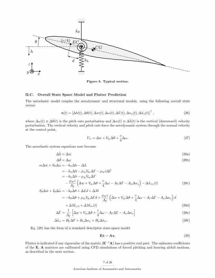
We focus here on the typical section (Fig. 3), as used frequently in the aeroelasticity community. UsingHamilton’s equation and Lagrangian mechanics, the equations of motion of an airfoil in heave and pitchmotion are found to be44,45

m∆h+ kh∆h+ Sθ∆θ = −∆L (25a)

Sθ∆h+ kθ∆θ + Iθ∆θ = ∆M (25b)

where here we define ∆h to be the heave perturbation, defined positive downward, and ∆θ to be the pitchangle perturbation, defined positive clockwise. m is the total mass/span of the section, Sθ ≡ (xcg−xea)mis the mass unbalance/span, where xcg and xea are the distances of the center of gravity and elastic center,respectively, from the leading edge. Iθ is the moment of inertia/span around the elastic axis. Finally, khis the heave displacement spring constant/span, and kθ is the torsional spring constant/span. The pitchingmoment equation (25b) is constructed about the elastic axis (or shear center) location, defined to be adistance d from the quarter chord point.

6 of 20


d

θ

h

EC(c/4)

CG

kθ

khz

xy

Figure 3. Typical section.

II.C. Overall State Space Model and Flutter Prediction

The aeroelastic model couples the aerodynamic and structural models, using the following overall statevector:

x(t) = [∆h(t),∆θ(t),∆w(t),∆ω(t),∆Γ(t),∆κx(t),∆κx(t)]>, (26)

where ∆ω(t) ≡ ∆θ(t) is the pitch rate perturbation and ∆w(t) ≡ ∆h(t) is the vertical (downward) velocityperturbation. The vertical velocity and pitch rate force the aerodynamic system through the normal velocityat the control point,

Un = ∆w + V∞∆θ +c

4∆ω. (27)

The aeroelastic system equations now become

∆h = ∆w (28a)

∆θ = ∆ω (28b)

m∆w + Sθ∆ω = −kh∆h−∆L

= −kh∆h− ρ∞V∞∆Γ− ρ∞c∆Γ

= −kh∆h− ρ∞V∞∆Γ

− ρ∞c

AΓ

(∆w + V∞∆θ +

c

4∆ω −AΓ∆Γ−Aκ∆κx

)−∆Lnc(t) (28c)

Sθ∆w + Iθ∆ω = −kθ∆θ + ∆Ld+ ∆M

= −kθ∆θ + ρ∞V∞∆Γd+ρ∞c

AΓ

(∆w + V∞∆θ +

c


)d

+ ∆Mc/4 + ∆Mnc(t) (28d)

∆Γ =1

AΓ

[∆w + V∞∆θ +

c


](28e)

∆κx = BΓ∆Γ +Bκ∆κx +Bκ∆κx. (28f)

Eq. (28) has the form of a standard descriptor state-space model

Ex = Ax. (29)

Flutter is indicated if any eigenvalue of the matrix (E−1A) has a positive real part. The unknown coefficientsof the E, A matrices are calibrated using CFD simulations of forced pitching and heaving airfoil motions,as described in the next section.

7 of 20


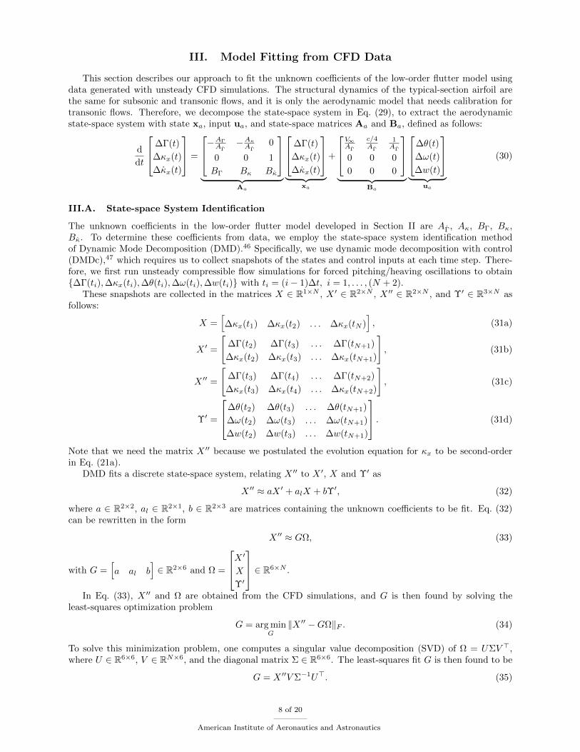
III. Model Fitting from CFD Data

This section describes our approach to fit the unknown coefficients of the low-order flutter model usingdata generated with unsteady CFD simulations. The structural dynamics of the typical-section airfoil arethe same for subsonic and transonic flows, and it is only the aerodynamic model that needs calibration fortransonic flows. Therefore, we decompose the state-space system in Eq. (29), to extract the aerodynamicstate-space system with state xa, input ua, and state-space matrices Aa and Ba, defined as follows:

d

dt

∆Γ(t)

∆κx(t)

∆κx(t)

=

−AΓ

AΓ−AκAΓ

0

0 0 1

BΓ Bκ Bκ

︸︷︷︸

Aa

∆Γ(t)

∆κx(t)

∆κx(t)

︸︷︷︸

xa

+

V∞AΓ

c/4AΓ

1AΓ

0 0 0

0 0 0

︸︷︷︸

Ba

∆θ(t)

∆ω(t)

∆w(t)

︸︷︷︸

ua

(30)

III.A. State-space System Identification

The unknown coefficients in the low-order flutter model developed in Section II are AΓ, Aκ, BΓ, Bκ,Bκ. To determine these coefficients from data, we employ the state-space system identification methodof Dynamic Mode Decomposition (DMD).46 Specifically, we use dynamic mode decomposition with control(DMDc),47 which requires us to collect snapshots of the states and control inputs at each time step. There-fore, we first run unsteady compressible flow simulations for forced pitching/heaving oscillations to obtain∆Γ(ti),∆κx(ti),∆θ(ti),∆ω(ti),∆w(ti) with ti = (i− 1)∆t, i = 1, . . . , (N + 2).

These snapshots are collected in the matrices X ∈ R1×N , X ′ ∈ R2×N , X ′′ ∈ R2×N , and Υ′ ∈ R3×N asfollows:

X =[∆κx(t1) ∆κx(t2) . . . ∆κx(tN )

], (31a)

X ′ =

[∆Γ(t2) ∆Γ(t3) . . . ∆Γ(tN+1)

∆κx(t2) ∆κx(t3) . . . ∆κx(tN+1)

], (31b)

X ′′ =

[∆Γ(t3) ∆Γ(t4) . . . ∆Γ(tN+2)

∆κx(t3) ∆κx(t4) . . . ∆κx(tN+2)

], (31c)

Υ′ =

∆θ(t2) ∆θ(t3) . . . ∆θ(tN+1)

∆ω(t2) ∆ω(t3) . . . ∆ω(tN+1)

∆w(t2) ∆w(t3) . . . ∆w(tN+1)

. (31d)

Note that we need the matrix X ′′ because we postulated the evolution equation for κx to be second-orderin Eq. (21a).

DMD fits a discrete state-space system, relating X ′′ to X ′, X and Υ′ as

X ′′ ≈ aX ′ + alX + bΥ′, (32)

where a ∈ R2×2, al ∈ R2×1, b ∈ R2×3 are matrices containing the unknown coefficients to be fit. Eq. (32)can be rewritten in the form

X ′′ ≈ GΩ, (33)

with G =[a al b

]∈ R2×6 and Ω =

X ′XΥ′

∈ R6×N .

In Eq. (33), X ′′ and Ω are obtained from the CFD simulations, and G is then found by solving theleast-squares optimization problem

G = arg minG

‖X ′′ −GΩ‖F . (34)

To solve this minimization problem, one computes a singular value decomposition (SVD) of Ω = UΣV >,where U ∈ R6×6, V ∈ RN×6, and the diagonal matrix Σ ∈ R6×6. The least-squares fit G is then found to be

G = X ′′V Σ−1U>. (35)

8 of 20


In contrast to the reduced-order modeling approach where DMD is typically used, we do not truncate thesingular values in Σ when computing G. In reduced-order modeling, the row dimension of the snapshotmatrices is the total number of states in the CFD model (typically 104 or higher), and DMD is used toidentify a model of much lower order. In contrast, in this system identification setting, we construct thedata matrices X, X ′, X ′′, and Υ′ with our six physical low-order quantities, such that the state dimensionof the DMD representation is already at the desired number.

The matrices a, al, and b are found by decomposing the linear operator U as[a, al, b

]≈[X ′′V Σ−1U>1 , X ′′V Σ−1U>2 , X ′′V Σ−1U>3

], (36)

where U1 ∈ R6×2, U2 ∈ R6×1, U3 ∈ R6×3 are the first two columns of U , the third column of U , and the lastthree columns of U .

Finally, we relate the discrete state-space matrices a, al, b to the continuous state-space matrices Aa andBa in Eq. (30) using Tustin’s method.48

The process described in this section allows for fitting one state space model for one particular freestreamMach number, airfoil and baseline lift coefficient. We would like to characterize the flutter boundary for arange of Mach numbers, airfoil thicknesses, and baseline lift coefficients. Therefore, the method describedin this section is used to find the aerodynamic state space matrices for a set of freestream Mach numbers,baseline lift coefficients, and different thicknesses of the same airfoil family. Splines are then fit for theentries in the aerodynamic state space matrices to find a low-order model at an interpolatory Mach number,baseline lift coefficient, and/or airfoil thickness.

III.B. CFD Data Generation

We fit the aerodynamic part of the state-space system using data from CFD solutions. Throughout this work,we use the SU2 tool suite.49 SU2 is a multi-purpose PDE solver, and specifically developed with aerospaceapplications in mind, such as unsteady compressible flow over an airfoil. For CFD applications, SU2 employsa finite volume method with standard edge-based structure on a dual grid. For unsteady simulations it usesa dual time-stepping strategy for high-order accuracy in time.50

Two changes to SU2 were necessary for this work. First, the parameters of our problem (κx, Γ) arecomputed by post-processing SU2 solutions. The circulation Γ(t) is defined as

Γ(t) ≡∫∫

ω(t) · y dA =

∮V(t) · dl. (37)

If this line integral is computed sufficiently close to the airfoil, it is more accurate than integrating thevorticity, because this is less susceptible to round-off errors and noise in the gradient computation. Notethat we need to choose the contour for the line integral to exclude the wake, such that we compute thecirculation without including shed vorticity. This is illustrated in Fig. 4(c).

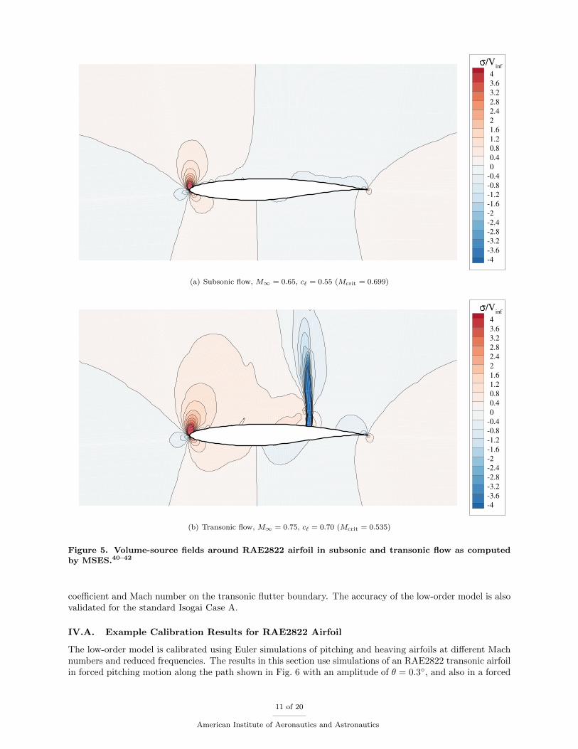
Computing the x-doublet through integration of the divergence of the velocity field is even more problem-atic, because the extrema in the volume-source field are highly localized. As an example, the volume-sourcefield around the RAE2822 airfoil in subsonic and transonic flow is shown in Fig. 5 for different lift coefficients,as computed with MSES.40–42 Using the contour shown in Fig. 4(b), the x-doublet is computed by evaluating

κx(t) = −∫∫

x∇ ·V(t) dA = −∮xV(t) · n ds+

∫∫U(t) dA

= −∮x [ V(t)−V∞] · n ds+

∫∫[U(t)− U∞] dA, (38)

where U is the velocity in the freestream x-direction. The final expression for κx(t) subtracts off V∞ tominimize cancellation errors.

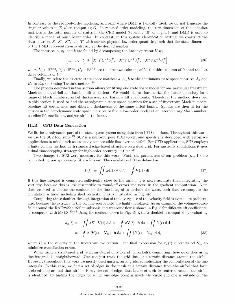
When using a structured grid (e.g., an O-grid or a C-grid for airfoils), computing these quantities usingline integrals is straightforward. One can just track the grid lines at a certain distance around the airfoil.However, throughout this work we mostly used unstructured grids, complicating the computation of the lineintegrals. In this case, we find a set of edges in the mesh at a certain distance from the airfoil that forma closed loop around that airfoil. First, the set of edges that intersect a circle centered around the airfoilis identified, by finding the edges for which one edge point is inside the circle and one is outside on the

9 of 20


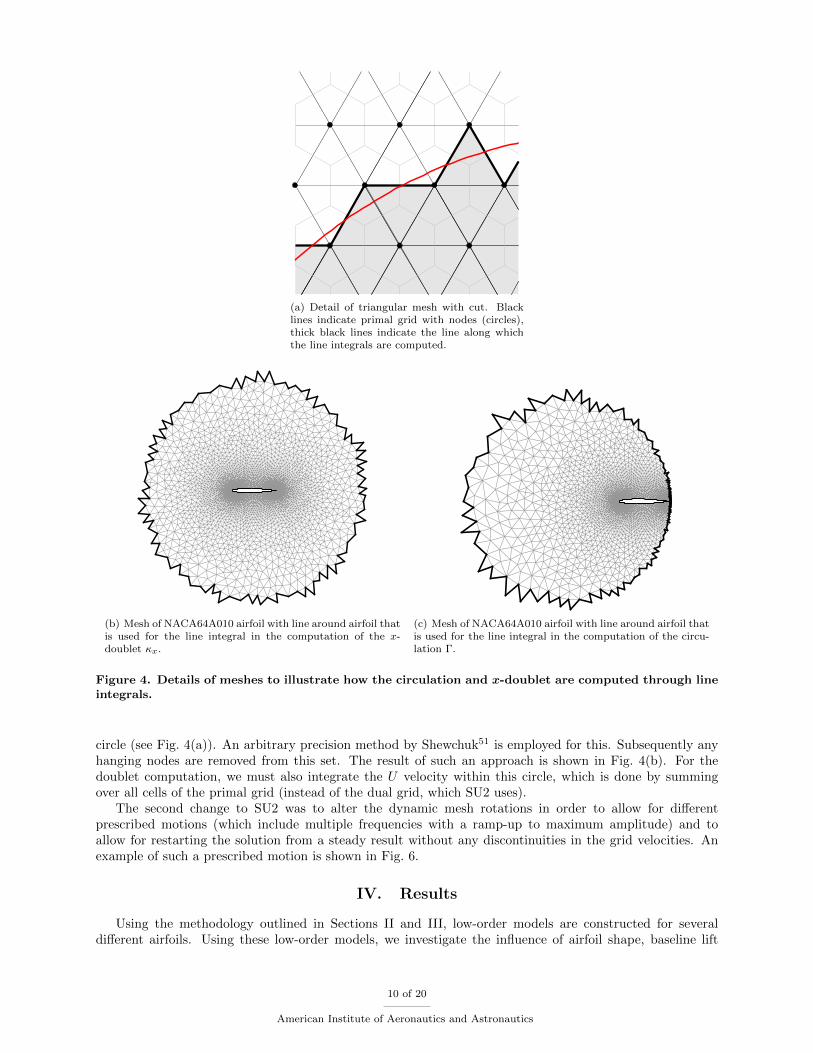
(a) Detail of triangular mesh with cut. Blacklines indicate primal grid with nodes (circles),thick black lines indicate the line along whichthe line integrals are computed.

(b) Mesh of NACA64A010 airfoil with line around airfoil thatis used for the line integral in the computation of the x-doublet κx.

(c) Mesh of NACA64A010 airfoil with line around airfoil thatis used for the line integral in the computation of the circu-lation Γ.

Figure 4. Details of meshes to illustrate how the circulation and x-doublet are computed through lineintegrals.

circle (see Fig. 4(a)). An arbitrary precision method by Shewchuk51 is employed for this. Subsequently anyhanging nodes are removed from this set. The result of such an approach is shown in Fig. 4(b). For thedoublet computation, we must also integrate the U velocity within this circle, which is done by summingover all cells of the primal grid (instead of the dual grid, which SU2 uses).

The second change to SU2 was to alter the dynamic mesh rotations in order to allow for differentprescribed motions (which include multiple frequencies with a ramp-up to maximum amplitude) and toallow for restarting the solution from a steady result without any discontinuities in the grid velocities. Anexample of such a prescribed motion is shown in Fig. 6.

IV. Results

Using the methodology outlined in Sections II and III, low-order models are constructed for severaldifferent airfoils. Using these low-order models, we investigate the influence of airfoil shape, baseline lift

10 of 20


/Vinf

4

3.6

3.2

2.8

2.4

2

1.6

1.2

0.8

0.4

0

0.4

0.8

1.2

1.6

2

2.4

2.8

3.2

3.6

4

(a) Subsonic flow, M∞ = 0.65, c` = 0.55 (Mcrit = 0.699)

/Vinf

4

3.6

3.2

2.8

2.4

2

1.6

1.2

0.8

0.4

0

0.4

0.8

1.2

1.6

2

2.4

2.8

3.2

3.6

4

(b) Transonic flow, M∞ = 0.75, c` = 0.70 (Mcrit = 0.535)

Figure 5. Volume-source fields around RAE2822 airfoil in subsonic and transonic flow as computedby MSES.40–42

coefficient and Mach number on the transonic flutter boundary. The accuracy of the low-order model is alsovalidated for the standard Isogai Case A.

IV.A. Example Calibration Results for RAE2822 Airfoil

The low-order model is calibrated using Euler simulations of pitching and heaving airfoils at different Machnumbers and reduced frequencies. The results in this section use simulations of an RAE2822 transonic airfoilin forced pitching motion along the path shown in Fig. 6 with an amplitude of θ = 0.3, and also in a forced

11 of 20


0 5 10 15

-0.3

-0.2

-0.1

0

0.1

0.2

0.3

Figure 6. Example of forced pitching oscillation.

heaving motion using a similar trajectory for h with an amplitude of h/V∞ = 0.005.First, we show the results of just the SU2 forced-heaving simulations for different Mach numbers in

Figures 7 and 8. Both the phase and the magnitude variation of the circulation and the x-doublet are seento significantly depend on the forcing reduced frequency ω, and its effect varies with the baseline Machnumber M∞. At the higher transonic Mach number, the dependence of the x-doublet phase on frequency isespecially strong. A physical explanation of this behavior is that the delays in propagation of the shock andacoustic waves which comprise the σ field variation will be strongly affected by the size of the supersoniczone, and hence by M∞.

These CFD results for different Mach numbers and different reduced frequencies are then used to calibratea low-order model. In this work, we focus on fitting one low-order model per Mach number for reducedfrequencies in the range of ω = 0.05 to ω = 0.40. In the DMD formulation of Section III, we require that allCFD simulations use the same fixed time step ∆t. Therefore, the low frequency simulations use more timesteps than the high frequency simulations. Throughout this work, we set the time step such that for thehighest reduced frequency 40 time steps per period are used.

For the calibration we combine the forced pitching and heaving simulations to yield one fit per Machnumber and airfoil. Applying the DMD method of Section III to these CFD results yields the fits shown inFigures 9 and 10 for pitching motion, and Fig. 11 for heaving motion. The low-order model captures thecirculation response quite accurately. Capture of the x-doublet response is quite reasonable as well, exceptfor the final part after we stop forcing the airfoil. This is likely due to the numerical noise in the SU2computation, which then also throws off the fit.

h/V∞ ×10-3

-6 -4 -2 0 2 4 6

Circu

lationstrength,Γ=

2Γ

V∞c

0.53

0.54

0.55

0.56

0.57

0.58

0.59

0.6

0.61

ω = 0.05ω = 0.10ω = 0.20ω = 0.30

(a) Subsonic (α0 = 1.5, M∞ = 0.5)

h/V∞ ×10-3

-6 -4 -2 0 2 4 6

Circu

lationstrength,Γ=

2Γ

V∞c

0.8

0.82

0.84

0.86

0.88

0.9

0.92

ω = 0.05ω = 0.10ω = 0.20ω = 0.30

(b) Transonic (α0 = 1.5, M∞ = 0.75)

Figure 7. Phase diagram of Γ for forced heaving at different reduced frequencies for subsonic andtransonic flow.

12 of 20


h/V∞ ×10-3

-6 -4 -2 0 2 4 6

x-doubletstrength,κx=

κx

V∞c2

0.032

0.033

0.034

0.035

0.036

ω = 0.05ω = 0.10ω = 0.20ω = 0.30

(a) Subsonic (α0 = 1.5, M∞ = 0.5)

h/V∞ ×10-3

-6 -4 -2 0 2 4 6

x-doubletstrength,κx=

κx

V∞c2

0.37

0.38

0.39

0.4

0.41

0.42

0.43

0.44

ω = 0.05ω = 0.10ω = 0.20ω = 0.30

(b) Transonic (α0 = 1.5, M∞ = 0.75)

Figure 8. Phase diagram of κx for forced heaving at different reduced frequencies for subsonic andtransonic flow.

We also show the errors in the fit for different Mach numbers in Tables 1 and 2. The error in each stateis computed as

εi =‖xi,DMD − xi,SU2‖2

‖xi,SU2‖2. (39)

The results in Tables 1 and 2 confirm that the fit for circulation is significantly better than the fit for thex-doublet.

-0.4 -0.3 -0.2 -0.1 0 0.1 0.2 0.3 0.4

-0.025

-0.02

-0.015

-0.01

-0.005

0

0.005

0.01

0.015

0.02

0.025

(a) Circulation strength

-0.4 -0.3 -0.2 -0.1 0 0.1 0.2 0.3 0.4

-8

-6

-4

-2

0

2

4

6

810

-3

(b) x-doublet strength

Figure 9. Comparison of phase diagrams between SU2 results and low-order model for forced pitchingoscillations at ω = 0.35 for M∞ = 0.6 for the RAE2822 airfoil with α0 = 1.5 (Mcrit = 0.648).

The goal of a calibrated low-order model is to be predictive at different frequencies. We calibrate onelow-order model for M∞ = 0.30 and one low-order model for M∞ = 0.70, and test these low-order modelsat frequencies that were not part of the frequencies used for calibration. Tables 3 and 4 show the accuracyof the DMD fits for these Mach numbers. We see that the accuracy for these frequencies is quite similar tothe accuracy for frequencies that were part of the calibration (Tables 1 and 2).

13 of 20


0 5 10 15

-0.03

-0.02

-0.01

0

0.01

0.02

0.03


0 5 10 15

-0.01

-0.005

0

0.005

0.01


Figure 10. Comparison of time series between SU2 results and low-order model for forced pitchingoscillations at ω = 0.35 for M∞ = 0.6 for the RAE2822 airfoil with α0 = 1.5 (Mcrit = 0.648).

-6 -4 -2 0 2 4 6

10-3

-0.025

-0.02

-0.015

-0.01

-0.005

0

0.005

0.01

0.015

0.02

0.025


-6 -4 -2 0 2 4 6

10-3

-5

-4

-3

-2

-1

0

1

2

3

4

510

-3


Figure 11. Comparison of phase diagrams between SU2 results and low-order model for forced heavingoscillations at ω = 0.25 for M∞ = 0.6 for the RAE2822 airfoil with α0 = 1.5 (Mcrit = 0.648).

Table 1. Accuracy of DMD fit forforced pitching oscillations at M∞ = 0.30for RAE2822 airfoil with α0 = 1.5

(Mcrit = 0.648).

ω Error Γ Error κx

0.05 2.8% 7.7%

0.10 2.5% 5.7%

0.15 2.9% 11.5%

0.20 2.7% 16.6%

0.25 2.3% 16.2%

0.30 1.5% 12.1%

0.35 1.3% 13.0%

0.40 3.9% 19.5%

Table 2. Accuracy of DMD fit forforced pitching oscillations at M∞ = 0.70for RAE2822 airfoil with α0 = 1.5

(Mcrit = 0.648).


0.05 4.9% 4.1%

0.10 3.8% 5.9%

0.15 2.5% 14.4%

0.20 2.8% 4.8%

0.25 5.8% 12.4%

0.30 3.6% 16.1%

0.35 1.5% 12.9%

0.40 5.8% 16.3%

We fit low-order models for different freestream Mach numbers to investigate the effect of compressibility

14 of 20


Table 3. Accuracy of DMD fit for forcedpitching oscillations at frequencies thatwere not part of the DMD calibration(M∞ = 0.30 for RAE2822 airfoil withα0 = 1.5, Mcrit = 0.648).


0.125 2.7% 8.5%

0.175 2.9% 14.4%

0.225 2.5% 17.1%

0.275 1.9% 14.5%

0.325 1.1% 10.9%

0.375 2.4% 16.7%

Table 4. Accuracy of DMD fit for forcedpitching oscillations at frequencies thatwere not part of the DMD calibration(M∞ = 0.70 for RAE2822 airfoil withα0 = 1.5, Mcrit = 0.648).


0.125 3.6% 17.2%

0.175 2.2% 9.7%

0.225 4.9% 6.6%

0.275 4.9% 19.0%

0.325 2.4% 13.2%

0.375 3.4% 9.8%

0 0.05 0.1 0.15 0.2 0.25 0.3 0.35 0.42

4

6

8

10

12

(a) Magnitude

0 0.05 0.1 0.15 0.2 0.25 0.3 0.35 0.4-80

-70

-60

-50

-40

-30

-20

-10

0

(b) Phase

Figure 12. Bode plot of transfer function between non-dimensional circulation (2Γ/V∞c) and pitchangle θ for different Mach numbers for the RAE2822 airfoil with α0 = 1.5 (Mcrit = 0.648).

on the aerodynamic response of the airfoil. The effect of Mach number is shown by the magnitude and phaseof the transfer function between circulation and the pitching angle θ in Fig. 12, where we also show theresult for Theodorsen’s theory. We see that the magnitude of the transfer function is strongly dependent onMach number, as expected, but that the Mach number influence becomes smaller as the reduced frequencyincreases. The magnitude of the transfer function is also quite different between subsonic and transonicMach numbers. Furthermore, the phase lag increases with subsonic Mach number and the Mach numberdependence becomes stronger as the reduced frequency increases. For high transonic Mach numbers (e.g.,M∞ = 0.85), however, the phase lag suddenly becomes smaller. The trends in these Bode plots are similarto Theodorsen theory, but the values are noticeable different, even for low Mach numbers. This is likely dueto considering an airfoil with thickness rather than a flat plate.

This low-order model can be used to investigate the effect of Mach number on the flutter boundary ofthe RAE2822 airfoil. Low-order models of the form Eq. (30) are fit using DMD at different freestream Machnumbers. For a given Mach number, the aerodynamic low-order model is coupled to the structural model—with airfoil parameters as listed in Table 5—to obtain the full aeroelastic state space model in Eq. (30). Here,we focus on the flutter speed as a function of the center of gravity position. The eigenvalues of (E−1A) fora given xcg are a function of V∞. A bisection method is used to find that flutter speed index Vµ for whichthe aeroelastic system becomes unstable, the results are shown in Fig. 13. The flutter speed index Vµ is anondimensionalization of the freestream velocity at which flutter occurs, and is defined as Vµ = 2V∞/

√µωθ c.

This bisection search is performed online and only involves solving 7× 7 eigenvalue problems. Constructingone flutter boundary in Fig. 13 for sixty different xcg locations therefore only takes ∼0.1 s.

Fig. 13 shows that for xcg far forward—or low reduced frequency—a higher subsonic Mach number

15 of 20


lowers the flutter speed. However, as the center of gravity moves aft—at high reduced frequencies—a highersubsonic Mach number increases the flutter speed. The behavior for transonic Mach numbers is quitedifferent, especially for xcg far forward. For instance, for xcg far forward, the flutter speed for M∞ = 0.80and M∞ = 0.85 is higher than for M∞ = 0.70, which is classic transonic flutter behavior and commonlydescribed as the “transonic dip”.

Airfoil parameter

RAE2822 (α0 = 1.5, Mcrit = 0.648)

Apparent-mass ratio µ = 4m/πρ∞c2 4.16

Inertia/mass ratio r2θ = 4Iθ/mc2 1.60

Elastic axis position xea/c 0.50

In-vacuo heavenatural frequency

ωh =√kh/m

√50.0

In-vacuo pitchnatural frequency

ωθ =√kθ/Iθ

√400

Table 5. Airfoil parameters used for fluttercalculations in Fig. 13, from Ref. 52.

0.34 0.36 0.38 0.4 0.42 0.44 0.46 0.48 0.5

0.6

0.8

1

1.2

1.4

1.6

1.8

2

2.2

Figure 13. Flutter speed versus xcg/c positions fordifferent freestream Mach numbers.

IV.B. Validation — Isogai Case A

0.1 0.2 0.3 0.4 0.5 0.6 0.7 0.8 0.9

0

0.5

1

1.5

2

2.5

3

Figure 14. Comparison of transonic flutter boundary for Isogai Case A20,53 as found by our methodand methods from literature.54–57 Mcrit = 0.762 for this case.

We validate the accuracy of the model using the standard Isogai case A.20,53 We compare our results forthe flutter boundary against four methods from the literature54–57 and against the flutter boundary foundusing SU2 (using the same mesh as was used to calibrate the model). We see that the agreement for thetransonic flow regime is quite good up to M∞ = 0.9. Isogai Case A is known for the characteristic S-shape ofits flutter boundary. For high transonic Mach numbers, the airfoil becomes unstable but if the flutter speedindex is increased further, it becomes stable again, until it finally becomes unstable again around Vµ ' 2.8.Our model will be implemented in an aircraft design code to yield flutter predictions of optimal designs. Agood design should never operate in the second stability region and therefore it is not a problem that themodel cannot capture this S-shape of the flutter boundary.

16 of 20


IV.C. Results Across Airfoil Shape Family

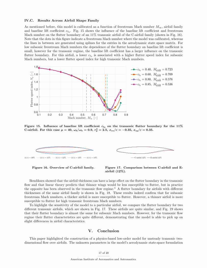
As mentioned before, this model is calibrated as a function of freestream Mach number M∞, airfoil familyand baseline lift coefficient c`0 . Fig. 15 shows the influence of the baseline lift coefficient and freestreamMach number on the flutter boundary of an 11% transonic airfoil of the C-airfoil family (shown in Fig. 16).Note that the dots in this figure indicate a freestream Mach number where the model was calibrated, whereasthe lines in between are generated using splines for the entries in the aerodynamic state space matrix. Forlow subsonic freestream Mach numbers the dependence of the flutter boundary on baseline lift coefficient issmall, however for the transonic regime, the baseline lift coefficient has a larger influence on the transonicflutter boundary. For this airfoil, a lower c`0 is associated with a higher flutter speed index for subsonicMach numbers, but a lower flutter speed index for high transonic Mach numbers.

0.1 0.2 0.3 0.4 0.5 0.6 0.7 0.8 0.9

0.6

0.8

1

1.2

1.4

1.6

1.8

Figure 15. Influence of baseline lift coefficient c`0 on the transonic flutter boundary for the 11%C-airfoil. For this case µ = 40, ωθ/ωh = 0.9, r2θ = 2.5, xea/c = −0.35, xcg/c = 0.35.

Figure 16. Overview of C-airfoil family. Figure 17. Comparison between C-airfoil and E-airfoil (12%).

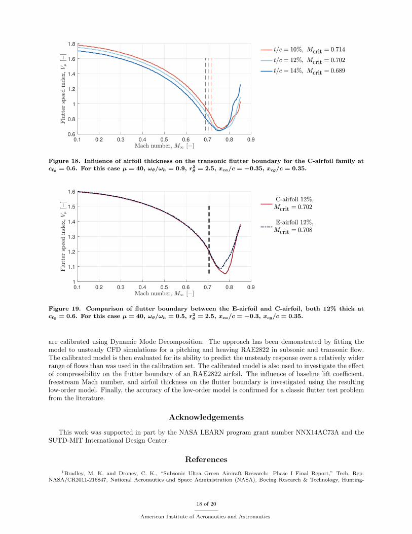
Bendiksen showed that the airfoil thickness can have a large effect on the flutter boundary in the transonicflow and that linear theory predicts that thinner wings would be less susceptible to flutter, but in practicethe opposite has been observed in the transonic flow regime.4 A flutter boundary for airfoils with differentthicknesses of the same airfoil family is shown in Fig. 18. These results indeed confirm that for subsonicfreestream Mach numbers, a thicker airfoil is more susceptible to flutter. However, a thinner airfoil is moresusceptible to flutter for high transonic freestream Mach numbers.

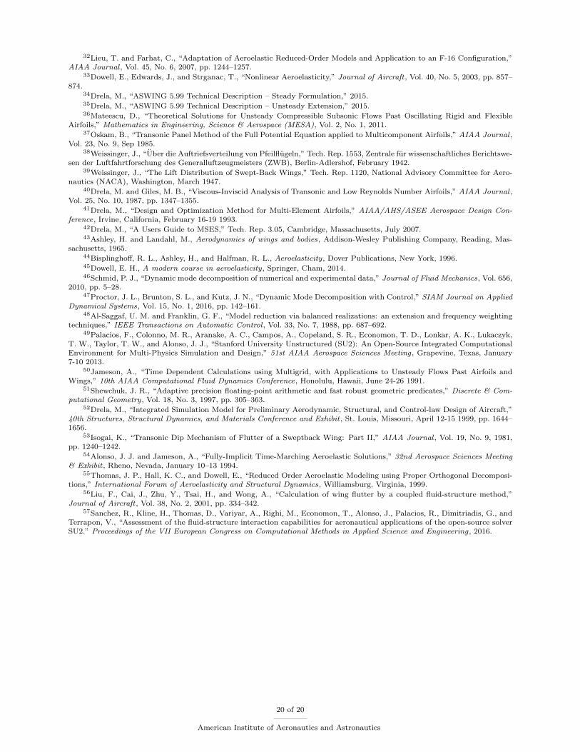
To highlight the sensitivity of the model to a particular airfoil, we compare the flutter boundary for twodifferent transonic airfoils, which are shown in Fig. 17. These airfoils are quite similar, and Fig. 19 showsthat their flutter boundary is almost the same for subsonic Mach numbers. However, for the transonic flowregime their flutter characteristics are quite different, demonstrating that the model is able to pick up onslight differences in airfoil characteristics.

V. Conclusion

This paper highlighted the construction of a physics-based low-order model for unsteady transonic two-dimensional flow over airfoils. The unknown parameters in the model’s aerodynamic state-space formulation

17 of 20


0.1 0.2 0.3 0.4 0.5 0.6 0.7 0.8 0.9

0.6

0.8

1

1.2

1.4

1.6

1.8

Figure 18. Influence of airfoil thickness on the transonic flutter boundary for the C-airfoil family atc`0 = 0.6. For this case µ = 40, ωθ/ωh = 0.9, r2θ = 2.5, xea/c = −0.35, xcg/c = 0.35.

0.1 0.2 0.3 0.4 0.5 0.6 0.7 0.8 0.9

1

1.1

1.2

1.3

1.4

1.5

1.6

Figure 19. Comparison of flutter boundary between the E-airfoil and C-airfoil, both 12% thick atc`0 = 0.6. For this case µ = 40, ωθ/ωh = 0.5, r2θ = 2.5, xea/c = −0.3, xcg/c = 0.35.

are calibrated using Dynamic Mode Decomposition. The approach has been demonstrated by fitting themodel to unsteady CFD simulations for a pitching and heaving RAE2822 in subsonic and transonic flow.The calibrated model is then evaluated for its ability to predict the unsteady response over a relatively widerrange of flows than was used in the calibration set. The calibrated model is also used to investigate the effectof compressibility on the flutter boundary of an RAE2822 airfoil. The influence of baseline lift coefficient,freestream Mach number, and airfoil thickness on the flutter boundary is investigated using the resultinglow-order model. Finally, the accuracy of the low-order model is confirmed for a classic flutter test problemfrom the literature.

Acknowledgements

This work was supported in part by the NASA LEARN program grant number NNX14AC73A and theSUTD-MIT International Design Center.

References

1Bradley, M. K. and Droney, C. K., “Subsonic Ultra Green Aircraft Research: Phase I Final Report,” Tech. Rep.NASA/CR2011-216847, National Aeronautics and Space Administration (NASA), Boeing Research & Technology, Hunting-

18 of 20


ton Beach, California, April 2011.2Kennedy, G. J., Kenway, G. K. W., and Martins, J. R. R. A., “Towards Gradient-Based Design Optimization of Flexible

Transport Aircraft with Flutter Constraints,” 15th AIAA/ISSMO Multidisciplinary Analysis and Optimization Conference,Atlanta, Georgia, June 16–20 2014.

3Mallik, W., Kapania, R. K., and Schetz, J. A., “Multidisciplinary Design Optimization of Medium-Range TransonicTruss-Braced Wing Aircraft with Flutter Constraint,” 54th AIAA/ASME/ASCE/AHS/ASC Structures, Structural Dynamics,and Materials Conference, April 8–11 2013.

4Bendiksen, O. O., “Review of Unsteady Transonic Aerodynamics: Theory and Applications,” Progress in AerospaceSciences, Vol. 47, No. 2, 2011, pp. 135–167.

5Mykytow, W. J., “A Brief Overview of Transonic Flutter Problems,” Unsteady Airloads in Separated and TransonicFlow, AGARD-CP-226, North Atlantic Treaty Organization, 1977.

6Farmer, M. G. and Itanson, P. W., “Comparison of Supercritical and Conventional Wing Flutter Characteristics,” Tech.Rep. TM X-72837, National Aeronautics and Space Administration (NASA), Langley Research Center, Hampton, Virginia,May 1976.

7Kholodar, D. B., Thomas, J. P., Dowell, E. H., and Hall, K. C., “Parametric Study of Flutter for an Airfoil in InviscidTransonic Flow,” Journal of Aircraft , Vol. 40, No. 2, 2003, pp. 303–313.

8Kholodar, D. B., Dowell, E. H., Thomas, J. P., and Hall, K. C., “Improved Understanding of Transonic Flutter: aThree-Parameter Flutter Surface,” Journal of Aircraft , Vol. 41, No. 4, 2004, pp. 911–917.

9Reddy, T. S. R., Srivastava, R., and Kaza, K. R. V., “The Effects of Rotational Flow, Viscosity, Thickness, and Shape onTransonic Flutter Dip Phenomena,” 29th AIAA/ASCE/AHS/ASC Structures, Structural Dynamics and Materials Conference,Williamsburg, Virginia, April 18–20 1988.

10Theodorsen, T., “General Theory of Aerodynamic Instability and the Mechanism of Flutter,” Tech. Rep. NACA-TR-496,National Aeronautics and Space Administration (NASA), Langley Aeronautical Lab, Hampton, Virginia, January 1935.

11Amiet, R. K., “Compressibility Effects in Unsteady Thin-Airfoil Theory,” AIAA Journal , Vol. 12, No. 2, 1974, pp. 252–255.

12Osborne, C., “Unsteady Thin-Airfoil Theory for Subsonic Flow,” AIAA Journal , Vol. 11, No. 2, 1973, pp. 205–209.13Miles, J. W., “On the Compressibility Correction for Subsonic Unsteady Flow,” Journal of the Aeronautical Sciences,

1950.14Possio, C., “L’Azione Aerodinamica sul Profilo Oscillante in un Fluido Comprimibile a Velocita Iposonora,” L’Aerotecnica,

Vol. 18, 1938, pp. 441–459.15Balakrishnan, A. V., “Unsteady Aerodynamics – Subsonic Compressible Inviscid Case,” Tech. Rep. NASA/CR-1999-

206583, National Aeronautics and Space Administration (NASA), Dryden Flight Research Center, Edwards, California, August1999.

16Lin, J. and Iliff, K. W., “Aerodynamic Lift and Moment Calculations Using a Closed-Form Solution of the Possio Equa-tion,” Tech. Rep. NASA/CR-2000-209019, National Aeronautics and Space Administration (NASA), Dryden Flight ResearchCenter, Edwards, California, April 2000.

17Garrick, I. E., “Bending-Torsion Flutter Calculations Modified by Subsonic Compressibility Corrections,” Tech. Rep. TN1034, National Advisory Committee for Aeronautics, Langley Memorial Aeronautical Laboratory, Langley Field, Virginia, May1946.

18Lomax, H., Heaslet, M. A., Fuller, F. B., and Sluder, L., “Two- and Three-Dimensional Unsteady Lift Problems inHigh-Speed Flight,” Tech. Rep. NACA TN 1077, National Advisory Committee for Aeronautics (NACA), 1952.

19Stahara, S. S. and Spreiter, J. R., “Development of a Nonlinear Unsteady Transonic Flow Theory,” Tech. Rep. NASA/CR-2258, National Aeronautics and Space Administration (NASA), Langley Research Center, Hampton, Virginia, June 1973.

20Isogai, K., “On the Transonic-dip Mechanism of Flutter of a Sweptback Wing,” AIAA Journal , Vol. 17, No. 7, 1979,pp. 793–795.

21Dowell, E., “A Simplified Theory of Oscillating Airfoils in Transonic Flow – Review and Extension,” 18thAIAA/ASCE/AHS/ASC Structures, Structural Dynamics and Materials Conference, San Diego, California, March 21-231977.

22Nixon, D., “Perturbation of a Discontinuous Transonic Flow,” AIAA Journal , Vol. 16, No. 1, 1978, pp. 47–52.23Leishman, J. G. and Nguyen, K. Q., “State-Space Representation of Unsteady Airfoil Behavior,” AIAA Journal , Vol. 28,

No. 5, 1990, pp. 836–844.24Benner, P., Gugercin, S., and Willcox, K., “A Survey of Projection-Based Model Reduction Methods for Parametric

Dynamical Systems,” SIAM Review , Vol. 57, No. 4, 2015, pp. 483–531.25Thomas, J. P., Dowell, E. H., and Hall, K. C., “Modeling Viscous Transonic Limit Cycle Oscillation Behavior using a

Harmonic Balance Approach,” Journal of Aircraft , Vol. 41, No. 6, 2004, pp. 1266–1274.26Sirovich, L., “Turbulence and the Dynamics of Coherent Structures. Part 1: Coherent Structures,” Quarterly of Applied

Mathematics, Vol. 45, No. 3, October 1987, pp. 561–571.27Berkooz, G., Holmes, P., and Lumley, J., “The Proper Orthogonal Decomposition in the Analysis of Turbulent Flows,”

Annual Review of Fluid Mechanics, Vol. 25, 1993, pp. 539–575.28Dowell, E. H. and Hall, K. C., “Modeling of Fluid-Structure Interaction,” Annual Review of Fluid Mechanics, Vol. 33,

No. 1, 2001, pp. 445–490.29Silva, W. A., “Application of Nonlinear Systems Theory to Transonic Unsteady Aerodynamic Responses,” Journal of

Aircraft , Vol. 30, No. 5, 1993, pp. 660–668.30Lucia, D. J., Beran, P. S., and Silva, W. A., “Reduced-Order Modeling: New Approaches for Computational Physics,”

Progress in Aerospace Sciences, Vol. 40, No. 1, 2004, pp. 51–117.31Thomas, J. P., Dowell, E. H., and Hall, K. C., “Three-Dimensional Transonic Aeroelasticity using Proper Orthogonal

Decomposition-Based Reduced-Order Models,” Journal of Aircraft , Vol. 40, No. 3, 2003, pp. 544–551.

19 of 20


32Lieu, T. and Farhat, C., “Adaptation of Aeroelastic Reduced-Order Models and Application to an F-16 Configuration,”AIAA Journal , Vol. 45, No. 6, 2007, pp. 1244–1257.

33Dowell, E., Edwards, J., and Strganac, T., “Nonlinear Aeroelasticity,” Journal of Aircraft , Vol. 40, No. 5, 2003, pp. 857–874.

34Drela, M., “ASWING 5.99 Technical Description – Steady Formulation,” 2015.35Drela, M., “ASWING 5.99 Technical Description – Unsteady Extension,” 2015.36Mateescu, D., “Theoretical Solutions for Unsteady Compressible Subsonic Flows Past Oscillating Rigid and Flexible

Airfoils,” Mathematics in Engineering, Science & Aerospace (MESA), Vol. 2, No. 1, 2011.37Oskam, B., “Transonic Panel Method of the Full Potential Equation applied to Multicomponent Airfoils,” AIAA Journal ,

Vol. 23, No. 9, Sep 1985.38Weissinger, J., “Uber die Auftriefsverteilung von Pfeilflugeln,” Tech. Rep. 1553, Zentrale fur wissenschaftliches Berichtswe-

sen der Luftfahrtforschung des Generalluftzeugmeisters (ZWB), Berlin-Adlershof, February 1942.39Weissinger, J., “The Lift Distribution of Swept-Back Wings,” Tech. Rep. 1120, National Advisory Committee for Aero-

nautics (NACA), Washington, March 1947.40Drela, M. and Giles, M. B., “Viscous-Inviscid Analysis of Transonic and Low Reynolds Number Airfoils,” AIAA Journal ,

Vol. 25, No. 10, 1987, pp. 1347–1355.41Drela, M., “Design and Optimization Method for Multi-Element Airfoils,” AIAA/AHS/ASEE Aerospace Design Con-

ference, Irvine, California, February 16-19 1993.42Drela, M., “A Users Guide to MSES,” Tech. Rep. 3.05, Cambridge, Massachusetts, July 2007.43Ashley, H. and Landahl, M., Aerodynamics of wings and bodies, Addison-Wesley Publishing Company, Reading, Mas-

sachusetts, 1965.44Bisplinghoff, R. L., Ashley, H., and Halfman, R. L., Aeroelasticity, Dover Publications, New York, 1996.45Dowell, E. H., A modern course in aeroelasticity, Springer, Cham, 2014.46Schmid, P. J., “Dynamic mode decomposition of numerical and experimental data,” Journal of Fluid Mechanics, Vol. 656,

2010, pp. 5–28.47Proctor, J. L., Brunton, S. L., and Kutz, J. N., “Dynamic Mode Decomposition with Control,” SIAM Journal on Applied

Dynamical Systems, Vol. 15, No. 1, 2016, pp. 142–161.48Al-Saggaf, U. M. and Franklin, G. F., “Model reduction via balanced realizations: an extension and frequency weighting

techniques,” IEEE Transactions on Automatic Control , Vol. 33, No. 7, 1988, pp. 687–692.49Palacios, F., Colonno, M. R., Aranake, A. C., Campos, A., Copeland, S. R., Economon, T. D., Lonkar, A. K., Lukaczyk,

T. W., Taylor, T. W., and Alonso, J. J., “Stanford University Unstructured (SU2): An Open-Source Integrated ComputationalEnvironment for Multi-Physics Simulation and Design,” 51st AIAA Aerospace Sciences Meeting, Grapevine, Texas, January7-10 2013.

50Jameson, A., “Time Dependent Calculations using Multigrid, with Applications to Unsteady Flows Past Airfoils andWings,” 10th AIAA Computational Fluid Dynamics Conference, Honolulu, Hawaii, June 24-26 1991.

51Shewchuk, J. R., “Adaptive precision floating-point arithmetic and fast robust geometric predicates,” Discrete & Com-putational Geometry, Vol. 18, No. 3, 1997, pp. 305–363.

52Drela, M., “Integrated Simulation Model for Preliminary Aerodynamic, Structural, and Control-law Design of Aircraft,”40th Structures, Structural Dynamics, and Materials Conference and Exhibit , St. Louis, Missouri, April 12-15 1999, pp. 1644–1656.

53Isogai, K., “Transonic Dip Mechanism of Flutter of a Sweptback Wing: Part II,” AIAA Journal , Vol. 19, No. 9, 1981,pp. 1240–1242.

54Alonso, J. J. and Jameson, A., “Fully-Implicit Time-Marching Aeroelastic Solutions,” 32nd Aerospace Sciences Meeting& Exhibit , Rheno, Nevada, January 10–13 1994.

55Thomas, J. P., Hall, K. C., and Dowell, E., “Reduced Order Aeroelastic Modeling using Proper Orthogonal Decomposi-tions,” International Forum of Aeroelasticity and Structural Dynamics, Williamsburg, Virginia, 1999.

56Liu, F., Cai, J., Zhu, Y., Tsai, H., and Wong, A., “Calculation of wing flutter by a coupled fluid-structure method,”Journal of Aircraft , Vol. 38, No. 2, 2001, pp. 334–342.

57Sanchez, R., Kline, H., Thomas, D., Variyar, A., Righi, M., Economon, T., Alonso, J., Palacios, R., Dimitriadis, G., andTerrapon, V., “Assessment of the fluid-structure interaction capabilities for aeronautical applications of the open-source solverSU2.” Proceedings of the VII European Congress on Computational Methods in Applied Science and Engineering, 2016.

20 of 20


Date post:	19-Jan-2020
Category:	Documents
Upload:	others
View:	23 times
Download:	0 times

Physics-Based Low-Order Model for Transonic Flutter...

Documents