PID CONTROLLER DESIGN FOR CONTROLLING DC MOTOR

SPEED USING MATLAB APPLICATION

MOHAMED FARID BIN MOHAMED FARUQ

UNIVERSITI MALAYSIA PAHANG

“I hereby acknowledge that the scope and quality of this thesis is qualified for the

award of the Bachelor Degree of Electrical Engineering (Power System)”

Signature : ______________________________________________

Name : AHMAD NOR KASRUDDIN BIN NASIR

Date : 11 NOVEMBER 2008

PID CONTROLLER DESIGN FOR CONTROLLING DC MOTOR

SPEED USING MATLAB APPLICATION

MOHAMED FARID BIN MOHAMED FARUQ

This thesis is submitted as partial fulfillment of the requirements for the award of the

Bachelor of Electrical Engineering (Power System)

Faculty of Electrical & Electronics Engineering

Universiti Malaysia Pahang

NOVEMBER, 2008

ii

“All the trademark and copyrights use herein are property of their respective owner.

References of information from other sources are quoted accordingly; otherwise the

information presented in this report is solely work of the author.”

Signature : ____________________________

Author : MOHAMED FARID BIN MOHAMED FARUQ

Date : 11 NOVEMBER 2008

iii

To my beloved mother, father and sister

iv

ACKNOWLEDGEMENT

In preparing this thesis, I was in contact with many people, researchers,

academicians, and practitioners. They have contributed towards my understanding

and thoughts. In particular, I wish to express my sincere appreciation to my thesis

supervisor, Mr. Ahmad Nor Kasruddin Bin Nasir, for encouragement, guidance,

critics and friendship. Without his continued support and interest, this thesis would

not have been the same as presented here. I would like to give my sincere

appreciation to all my friends and others who have provided assistance at various

occasions. Their views and tips are useful indeed. Unfortunately, it is not possible to

list all of them in this limited space. Finally to all my family members where without

them I would not be here.

v

ABSTRACT

This project is a simulation and experimental investigation into the

development of PID controller using MATLAB/SIMULINK software. The

simulation development of the PID controller with the mathematical model of DC

motor is done using Ziegler–Nichols method and trial and error method. The PID

parameter is to be tested with an actual motor also with the PID controller in

MATLAB/SIMULINK software. In order to implement the PID controller from the

software to the actual DC motor data acquisition is used. From the simulation and the

experiment, the result performance of the PID controller is compared in term of

response and the assessment is presented.

vi

ABSTRAK

Project in adalah penyelidikan secara simulasi dan eksperimen dalam

pembangunan pengawal PID mengunakan perisian MATLAB/SIMULINK.

Pembangunan simulasi pengawal PID dengan model matematik motor DC

mengunankan kaedah Ziegler–Nichols dan kaedah cuba dan jaya. Parameter

pengawal PID akan diuji dengan motor sebenar juga dengan pengawal PID

mengunakan perisian MATLAB/SIMULIN. Bagi mengaplikasikan pengawal PID

dari perisian kepada motor DC sebenar, data acquisition card di gunakan. Dari

simulasi dan eksperimen, keputusan kecekapan dari pengawal PID dibandingkan dari

segi respon dan analisis di lakukan dan dibentangkan.

vii

 

TABLE OF CONTENTS

CHAPTER TITLE PAGE

TITLE PAGE i

DECLARATION ii

DEDICATION iii

ACKNOWLEDGEMENT iv

ABSTRACT v

ABSTRAK vi

TABLE OF CONTENTS vii

LIST OF TABLES x

LIST OF FIGURES xi

LIST OF SYMBOLS xv

LIST OF APPENDICES xvi

I INTRODUCTION

1.1 Background of Project 1

1.2 Objective 2

1.3 Scope of Work 2

1.4 Problem Statement 3

viii

 

II LITERATURE REVIEW

2.1 Permanent Magnet Direct Current Motor 4

2.2 Control Theory 5

2.2.1 Closed-Loop Transfer Function 6

2.2.2 PID Controller 8

2.3 Pulse Width Modulation 9

2.4 MATLAB® and SIMULINK® 11

III METHODOLOGY

3.1 System Description 15

3.1.1 Mathematical Model 19

3.2 Data Acquisition 22

3.2.1 PCI-1710HG 24

3.2.1.1 Specification 25

3.2.1.2 Installation Guide 29

3.3 Real Time Computing 31

3.4 Real Time Window Target 32

3.4.1 Setup and Configuration 34

3.4.1.1 Compiler 34

3.4.1.2 Kernel Setup 35

3.4.1.3 Testing the Installation 37

3.4.2 Creating a Real Time Application 39

3.4.3 Entering Configuration Parameters for 47

Simulink

3.4.4 Entering Simulation Parameters for 49

Real-Time Workshop

3.4.5 Creating a Real-Time Application 51

3.4.6 Running a Real-Time Application 52

3.5 Driver 53

3.5.1 Geckodrive G340 54

ix

 

3.5.2 Alternative Driver IR2109 55

3.5 Project Planning 56

IV RESULT AND DISCUSSION

4.1 Controller Design 57

4.1.1 PID Controller 58

4.1.1.1 Zeigler Nichols Method 58

4.1.1.2 Trial and Error Method 59

4.2 Simulation without PID Controller 60

4.3 Simulation with PID Controller 61

4.4 Experiment without PID Controller 62

4.5 Experiments with PID Controller 66

V CONCLUSION AND RECOMENDATION

5.1 Conclusion 70

5.2 Future Recommendation 71

REFERENCES 73

APPENDICES

APPENDIX A 76

APPENDIX B 77

APPENDIX C 78

x

 

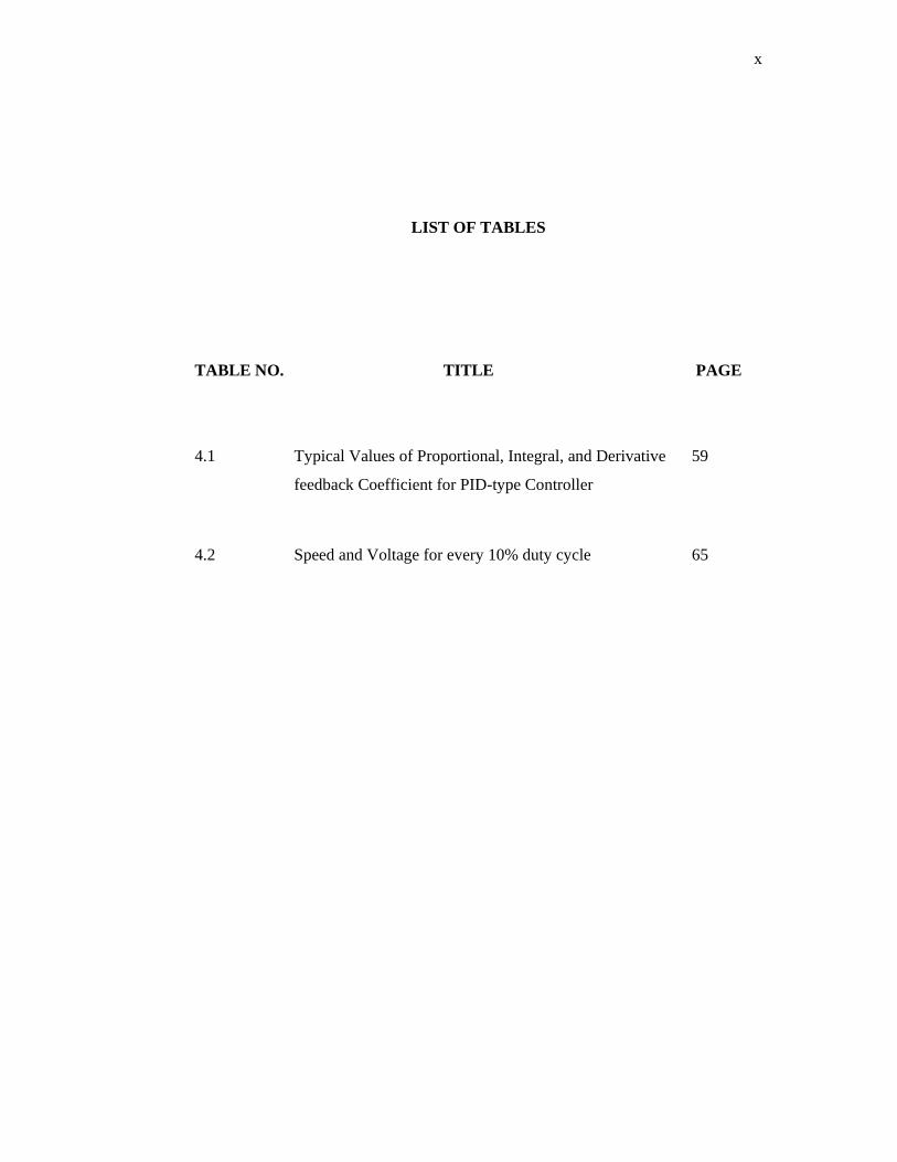
LIST OF TABLES

TABLE NO. TITLE PAGE

4.1 Typical Values of Proportional, Integral, and Derivative 59

feedback Coefficient for PID-type Controller

4.2 Speed and Voltage for every 10% duty cycle 65

xi

 

LIST OF FIGURE

FIGURE NO. TITLE PAGE

2.1 Concept of the Feedback Loop to Control the Dynamic 5

Behavior of the Reference

2.2 Closed-Loop Controller or Feedback Controller 7

2.3 A Square Wave, Showing the Definitions of ymin, ymax 9

and D

2.4 PWM Pulse Generate from Comparing Sinewave and 10

Sawtooth

2.7 MATLAB® Default Command Windows 12

2.8 SIMULINK® Running a Simulation of a Thermostat- 14

Controlled Heating System

3.1 Block Diagram of the System 15

3.2 Geckodrive G340 16

3.3 Alternative Driver (IR2109) 16

xii

 

3.4 Power Supply 16

3.5 Oscilloscope 16

3.6 Data Acquisition Card (PCI-1710HG) 16

3.7 Industrial Wiring Terminal Board with CJC Circuit 17

(PCLD-8710)

3.8 Personal Computer 17

3.9 Litton - Clifton Precision Servo DC Motor JDH-2250 18

3.10 Schematic Diagram of the DC Motor 19

3.11 Block Diagram of the Open-Loop Permanent-Magnet 21

DC Motor

3.12 Block Diagram of the Open-Loop Servo Actuated by 21

Permanent-Magnet DC Motor

3.13 Block Diagram of the Closed-Loop Servo with PID 22

Controller

3.14 Pin Assignment 27

3.15 Block Diagram of PCI-1710HG 28

3.16 PCI-1710HG Installation Flow Chart 30

3.17 Simulink Model rtvdp.mdl 37

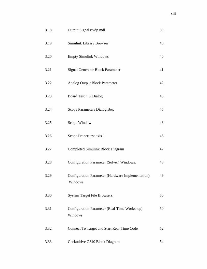
xiii

 

3.18 Output Signal rtvdp.mdl 39

3.19 Simulink Library Browser 40

3.20 Empty Simulink Windows 40

3.21 Signal Generator Block Parameter 41

3.22 Analog Output Block Parameter 42

3.23 Board Test OK Dialog 43

3.24 Scope Parameters Dialog Box 45

3.25 Scope Window 46

3.26 Scope Properties: axis 1 46

3.27 Completed Simulink Block Diagram 47

3.28 Configuration Parameter (Solver) Windows. 48

3.29 Configuration Parameter (Hardware Implementation) 49

Windows

3.30 System Target File Browsers. 50

3.31 Configuration Parameter (Real-Time Workshop) 50

Windows

3.32 Connect To Target and Start Real-Time Code 52

3.33 Geckodrive G340 Block Diagram 54

xiv

 

3.34 Typical Connections for IR2109 55

3.35 Flow Chart of Project 56

4.1 Simulink Block of PID Controller 58

4.2 Detailed Simulink Block of the System 60

4.3 Output of DC Motor without PID Controller 60

4.4 Detail Simulink Block of the System with PID Controller 61

4.5 Output of DC Motor without PID Controller 62

4.6 Simulink Block of Experiment without PID 63

4.7 10% Duty Cycle Pulse 63

4.8 50% Duty Cycle Pulse 64

4.9 90% Duty Cycle Pulse 64

4.10 Velocity Estimation 65

4.11 Complete Simulink Block of the Experiment 67

4.12 Velocity Decoder Subsystem Simulink Block 68

xv

LIST OF SYMBOLS

D - duty cycle

T - period

TL - load torque

Өr - angle

ωr - rotor angular displacement

ia - armature current

Ea - Induced emf

ka - back emf / torque constant

ra - armature resistance

La - armature inductance

J - moment of inertia

Bm - viscous friction coefficient

Tviscous - viscous friction torque

ua - armature voltage

kp - proportional coefficient

ki - integral coefficient

kd - derivative coefficient

Tocs - period of self-sustained oscillation

kpmax - critical value of proportional coefficient

xvi

LIST OF APPENDICES

APPENDIX TITLE PAGE

A Simulink Block of PID Control DC Motor (Simulation) 76

Simulink Block of DC Motor

Simulink Block of PID Controller

B Simulink Block of PID Control DC Motor (Experiment) 77

Simulink Block of Velocity Decoder

C Embedded MATLAB Function 78

MATLAB Command

 

 

 

CHAPTER 1

INTRODUCTION

1.1 Background of Project

Permanent magnet direct current motor (PMDC) have been widely use in

high-performance electrical drives and servo system. There are many difference DC

motor types in the market and all with it good and bad attributes. Such bad attribute

is the lag of efficiency. In order to overcome this problem a controller is introduce to

the system.

There are also many types of controller used in the industry, such controller is

PID controller. PID controller or proportional–integral–derivative controller is a

generic control loop feedback mechanism widely used in industrial control systems.

A PID controller attempts to correct the error between a measured process variable

and a desired set point by calculating and then outputting a corrective action that can

adjust the process accordingly. So by integrating the PID controller to the DC motor

were able to correct the error made by the DC motor and control the speed or the

position of the motor to the desired point or speed.

2

 

1.2 Objective

The objectives of this project are:

i. To fulfill the requirement for the subject BEE4712: Engineering Project.

ii. To explorer and apply the knowledge gain in lectures into practical

applications.

iii. To control the speed of DC motor with PID controller using

MATLAB/SIMULINK application.

iv. To design the PID controller and tune it using MATLAB/SIMULINK.

v. To compare and analyze the result between the simulation result using a DC

motor mathematical model in MATLAB/SIMULINK and the experimental

result using the actual motor.

1.3 Scope of Work

The scope of this project is;

i. Design and produce the simulation of the PID controller

ii. Simulate the PID controller with the modeling of the DC motor

iii. Implement the PID simulation with and actual DC motor

iv. The comparison of the simulation result with the actual DC motor

3

 

1.4 Problem Statement

The problem encounter when dealing with DC motor is the lag of efficiency

and losses. In order to eliminate this problem, controller is introduce to the system.

There’s few type of controller but in this project, PID controller is chosen as the

controller for the DC motor. This is because PID controller helps get the output,

where we want it in a short time, with minimal overshoot and little error.

 

 

 

CHAPTER 2

LITERATURE REVIEW

2.1 Permanent Magnet Direct Current Motor

A DC motor is designed to run on DC electric power [3]. An example is

Michael Faraday's homopolar motor, and the ball bearing motor. There are two types

of DC motor which are brush and brushless types, in order to create an oscillating

AC current from the DC source and internal and external commutation is use

respectively. So they are not purely DC machines in a strict sense [3].

A brushless DC motor (BLDC) is a synchronous electric motor which is

powered by direct-current electricity (DC) and which has an electronically controlled

commutation system, instead of a mechanical commutation system based on brushes

[4]. In such motors, current and torque, voltage and rpm are linearly related [4].

BLDC has its own advantages such as higher efficiency and reliability, reduced

noise, longer lifetime, elimination of ionizing sparks from the commutator, and

overall reduction of electromagnetic interference (EMI). With no windings on the

rotor, they are not subjected to centrifugal forces, and because the electromagnets are

located around the perimeter, the electromagnets can be cooled by conduction to the

motor casing, requiring no airflow inside the motor for cooling [4]. The disadvantage

5

is higher cost, because of two issues. First, it requires complex electronic speed

controller to run.

2.2 Control Theory

Control theory is an interdisciplinary branch of engineering and mathematics

that deals with the behavior of dynamical systems [7]. The desired output of a system

is called the reference [7]. When one or more output variables of a system need to

follow a certain reference over time, a controller manipulates the inputs to a system

to obtain the desired effect on the output of the system [7].

Figure 2.1 Concept of the Feedback Loop to Control the Dynamic Behavior of the

Reference

If we consider an automobile cruise control, it is design to maintain the speed of the

vehicle at a constant speed set by the driver. In this case the system is the vehicle. The

vehicle speed is the output and the control is the vehicle throttle which influences the engine

torque output. One way to implement cruise control is by locking the throttle at the desired

speed but when encounter a hill the vehicle will slow down going up and accelerate going

down. In fact, any parameter different than what was assumed at design time will

translate into a proportional error in the output velocity, including exact mass of the

6

vehicle, wind resistance, and tire pressure [7]. This type of controller is called

an open-loop controller because there is no direct connection between the output of

the system (the engine torque) and the actual conditions encountered; that is to say,

the system does not and cannot compensate for unexpected forces [7].

For a closed-loop control system, a sensor will monitor the vehicle speed and

feedback the data to its computer and continuously adjusting its control input or the

throttle as needed to ensure the control error to a minimum therefore maintaining the

desired speed of the vehicle. Feedback on how the system is actually performing

allows the controller (vehicle's on board computer) to dynamically compensate for

disturbances to the system, such as changes in slope of the ground or wind speed [7].

An ideal feedback control system cancels out all errors, effectively mitigating the

effects of any forces that may or may not arise during operation and producing a

response in the system that perfectly matches the user's wishes [7].

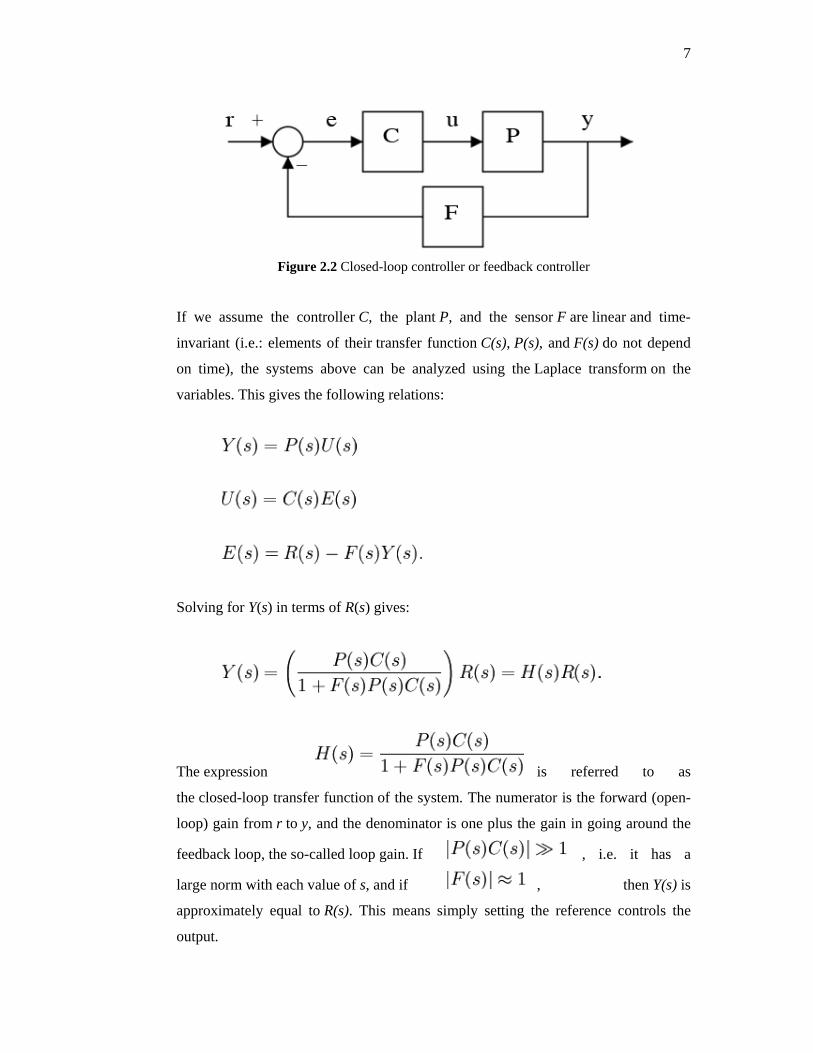
2.2.1 Closed-Loop Transfer Function

The output of the system y(t) is fed back through a sensor measurement F to

the reference value r(t). The controller C then takes the error e (difference) between

the reference and the output to change the inputs u to the system under control P.

This is shown in the figure. This kind of controller is a closed-loop controller or

feedback controller. This is called a single-input-single-output (SISO) control

system; MIMO (i.e. Multi-Input-Multi-Output) systems, with more than one

input/output, are common. In such cases variables are represented

through vectors instead of simple scalar values. For some distributed parameter

systems the vectors may be infinite-dimensional (typically functions).

7

Figure 2.2 Closed-loop controller or feedback controller

If we assume the controller C, the plant P, and the sensor F are linear and time-

invariant (i.e.: elements of their transfer function C(s), P(s), and F(s) do not depend

on time), the systems above can be analyzed using the Laplace transform on the

variables. This gives the following relations:

Solving for Y(s) in terms of R(s) gives:

The expression is referred to as

the closed-loop transfer function of the system. The numerator is the forward (open-

loop) gain from r to y, and the denominator is one plus the gain in going around the

feedback loop, the so-called loop gain. If , i.e. it has a

large norm with each value of s, and if , then Y(s) is

approximately equal to R(s). This means simply setting the reference controls the

output.

8

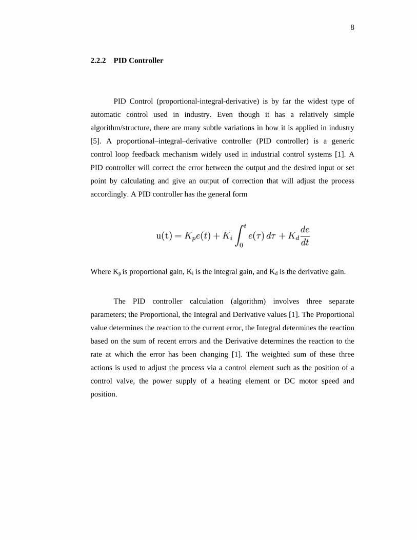
2.2.2 PID Controller

PID Control (proportional-integral-derivative) is by far the widest type of

automatic control used in industry. Even though it has a relatively simple

algorithm/structure, there are many subtle variations in how it is applied in industry

[5]. A proportional–integral–derivative controller (PID controller) is a generic

control loop feedback mechanism widely used in industrial control systems [1]. A

PID controller will correct the error between the output and the desired input or set

point by calculating and give an output of correction that will adjust the process

accordingly. A PID controller has the general form

Where Kp is proportional gain, Ki is the integral gain, and Kd is the derivative gain.

The PID controller calculation (algorithm) involves three separate

parameters; the Proportional, the Integral and Derivative values [1]. The Proportional

value determines the reaction to the current error, the Integral determines the reaction

based on the sum of recent errors and the Derivative determines the reaction to the

rate at which the error has been changing [1]. The weighted sum of these three

actions is used to adjust the process via a control element such as the position of a

control valve, the power supply of a heating element or DC motor speed and

position.

9

2.3 Pulse Width Modulation

Pulse-width modulation (PWM) of a signal or power source involves the

modulation of its duty cycle, to either convey information over a communications

channel or control the amount of power sent to a load.

Pulse-width modulation uses a square wave whose pulse width is modulated

resulting in the variation of the average value of the waveform. If we consider a

square waveform f(t) with a low value ymin, a high value ymax and a duty cycle D (see

figure 2.3), the average value of the waveform is given by:

Figure 2.3 A Square Wave, Showing the Definitions of ymin, ymax and D

As f(t) is a square wave, its value is ymax for and ymin for

. The above expression then becomes:

10

This latter expression can be fairly simplified in many cases where ymin = 0 as

. From this, it is obvious that the average value of the signal ( ) is

directly dependent on the duty cycle D.

The simplest way to generate a PWM signal is the intersective method, which

requires only a sawtooth or a triangle waveform (easily generated using a simple

oscillator) and a comparator. When the value of the reference signal (the green sine

wave in figure 2.4) is more than the modulation waveform (blue), the PWM signal

(magenta) is in the high state, otherwise it is in the low state.

Figure 2.4 PWM Pulse Generate from Comparing Sinewave and Sawtooth 

 

11

2.4 MATLAB and SIMULINK

MATLAB is a high-performance language for technical computing. It

integrates computation, visualization, and programming in an easy-to-use

environment where problems and solutions are expressed in familiar mathematical

notation. Typical uses include:

• Math and computation

• Algorithm development

• Data acquisition

• Modeling, simulation, and prototyping

• Data analysis, exploration, and visualization

• Scientific and engineering graphics

• Application development, including graphical user interface building

MATLAB is an interactive system whose basic data element is an array that

does not require dimensioning. This allows you to solve many technical computing

problems, especially those with matrix and vector formulations, in a fraction of the

time it would take to write a program in a scalar non-interactive language such as C

or Fortran.

The name MATLAB stands for matrix laboratory. MATLAB was originally

written to provide easy access to matrix software developed by the LINPACK and

EISPACK projects. Today, MATLAB engines incorporate the LAPACK and BLAS

libraries, embedding the state of the art in software for matrix computation.

MATLAB has evolved over a period of years with input from many users. In

university environments, it is the standard instructional tool for introductory and

advanced courses in mathematics, engineering, and science. In industry, MATLAB is

the tool of choice for high-productivity research, development, and analysis.

MATLAB features a family of add-on application-specific solutions called

toolboxes. Very important to most users of MATLAB, toolboxes allow you to learn

12

and apply specialized technology. Toolboxes are comprehensive collections of

MATLAB functions (M-files) that extend the MATLAB environment to solve

particular classes of problems. Areas in which toolboxes are available include signal

processing, control systems, neural networks, fuzzy logic, wavelets, simulation, and

many others.

When you start MATLAB, the MATLAB desktop appears, containing tools

(graphical user interfaces) for managing files, variables, and applications associated

with MATLAB. The following illustration shows the default desktop. You can

customize the arrangement of tools and documents to suit your needs.

 

 

Figure 2.7 MATLAB Default Command Windows

Simulink is software for modeling, simulating, and analyzing dynamic

systems. Simulink enables you to pose a question about a system, model it, and see

what happens.

13

With Simulink, you can easily build models from scratch, or modify existing

models to meet your needs. Simulink supports linear and nonlinear systems, modeled

in continuous time, sampled time, or a hybrid of the two. Systems can also be

multirate — having different parts that are sampled or updated at different rates.

Thousands of scientists and engineers around the world use Simulink® to

model and solve real problems in a variety of industries, including:

• Aerospace and Defense

• Automotive

• Communications

• Electronics and Signal Processing

• Medical Instrumentation

Model analysis tools include linearization and trimming tools, whichcan be accessed

from the MATLAB command line, plus the many tools in MATLAB and its

application toolboxes. Because MATLAB® and Simulink are integrated; you can

simulate, analyze, and revise your models in either environment at any point.

Simulink® is tightly integrated with MATLAB. It requires MATLAB to run,

depending on MATLAB to define and evaluate model and block parameters.

Simulink® can also utilize many MATLAB features. For example, Simulink can use

MATLAB to:

• Define model inputs.

• Store model outputs for analysis and visualization.

• Perform functions within a model, through integrated calls to MATLAB

operators and functions.

14

Figure 2.8 Simulink Running a Simulation of a Thermostat-Controlled Heating System

 

 

CHAPTER 3

METHODOLOGY

3.1 System Description

Figure 3.1 Block Diagram of the System

The system block diagram is as shown in Figure 3.1. It consist of 2 main

block (PC and Motor) that are connected through a driver and supplied by a power

supply. The control algorithm is builded in the Matlab/Simulink software and

compiled with Real-Time Window Target. The Real-Time Window Target Toolbox

include an analog input and analog output that provide connection between the data

acquisition card (PCI-1710HG) and the simulink model. For example, the speed of

the DC motor could be controlled by supplying certain voltage and frequency from

SPEED MEASUREMENT 

 

 

 

 

ENCORDER 

MOTOR 

PC SIMULINK  (REAL‐TIME  

WINDOW TARGET)  

DATA ACQUISITION CARD  

(PCI‐1710HG) 

POWER SUPPLY

DRIVER 

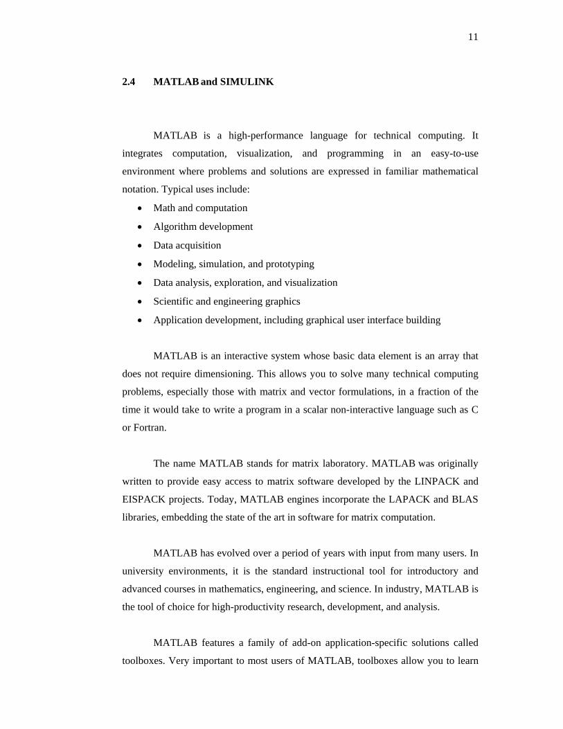
16

signal generator block to the analog output in Simulink. From the analog input, the

square received is displayed in a scope. The square wave pulse then is derived using

the velocity equation to get the velocity of the DC motor speed. The speed acquired

and the signal send can create a closed loop system with PID controller to control the

speed of the DC motor. Figure 3.2 to Figure 3.9 shows the DC motor, driver, and

other hardware used in this project and the DC motor specification.

 

Figure 3.2 Geckodrive G340 Figure 3.3 Alternative Driver (IR2109)

     Figure 3.4 Power Supply Figure 3.5 Oscilloscope

Figure 3.6 Data Acquisition Card (PCI-1710HG)

17

Figure 3.7 Industrial Wiring Terminal Board with CJC Circuit (PCLD-8710)

Figure 3.8 Personal Computer

18

Figure 3.9 Litton - Clifton Precision Servo DC Motor JDH-2250

Specification of JDH-2250

Torque Constant: 15.76 oz-in. / A

Back EMF: 11.65 VDC / KRPM

Peak Torque: 125 oz-in.

Cont. Torque: 16.5 oz-in.

Encoder: 250 counts / rev.

Channels: A, B in quadrature, 5 VDC input (no index)

Body Dimensions: 2.25" dia. x 4.35" L (includes encoder)

Shaft Dimensions: 8 mm x 1.0" L w/flat

19

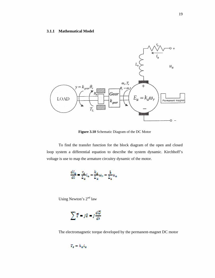
3.1.1 Mathematical Model

Figure 3.10 Schematic Diagram of the DC Motor

To find the transfer function for the block diagram of the open and closed

loop system a differential equation to describe the system dynamic. Kirchhoff’s

voltage is use to map the armature circuitry dynamic of the motor.

Using Newton’s 2nd law

The electromagnetic torque developed by the permanent-magnet DC motor

20

The viscous friction torque

The load torque is denoted as TL. Use the Newton’s second law, we have

The dynamics of the rotor angular displacement

To find the transfer function, the derived three first-order differential equation

and

Using the Laplace operator

21

From the transfer function, the block diagram of the permanent-magnet DC motor is

illustrated by Figure 3.11

Figure 3.11 Block Diagram of the Open-Loop Permanent-Magnet DC Motor

Figure 3.12 Block Diagram of the Open-Loop Servo Actuated by Permanent-Magnet DC

Motor

Using the linear PID controller

22

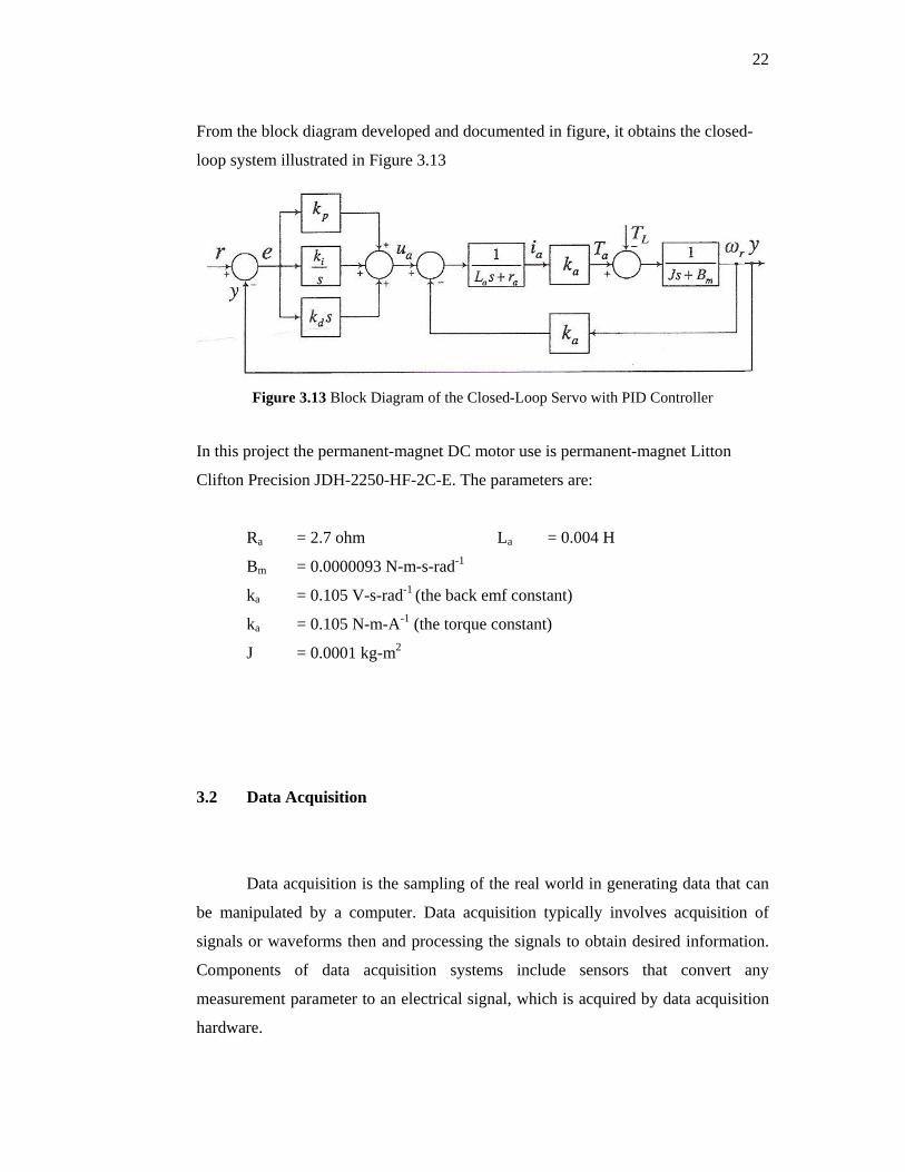
From the block diagram developed and documented in figure, it obtains the closed-

loop system illustrated in Figure 3.13

Figure 3.13 Block Diagram of the Closed-Loop Servo with PID Controller

In this project the permanent-magnet DC motor use is permanent-magnet Litton

Clifton Precision JDH-2250-HF-2C-E. The parameters are:

Ra = 2.7 ohm La = 0.004 H

Bm = 0.0000093 N-m-s-rad-1

ka = 0.105 V-s-rad-1 (the back emf constant)

ka = 0.105 N-m-A-1 (the torque constant)

J = 0.0001 kg-m2

3.2 Data Acquisition

Data acquisition is the sampling of the real world in generating data that can

be manipulated by a computer. Data acquisition typically involves acquisition of

signals or waveforms then and processing the signals to obtain desired information.

Components of data acquisition systems include sensors that convert any

measurement parameter to an electrical signal, which is acquired by data acquisition

hardware.

23

The acquired data from the data acquisition hardware are displayed,

analyzed, and stored on a computer, either using software, or custom displays and

control developed using programming languages such as BASIC, C, Fortran, Java,

Lisp, Pascal. Programming languages that used for data acquisition include, EPICS,

Lab VIEW, and MATLAB provides a programming language but also built-in

graphical tools and libraries for data acquisition and analysis.

Transducer is a device that converts physical property or phenomenon into

corresponding measurable electrical signal, such as voltage and current. The data

acquisition system ability to measure different phenomena depends on the

transducers to convert the physical phenomena into a signal measurable by the data

acquisition hardware. There are specific transducers for many different applications,

such as measuring temperature, pressure, or fluid flow. DAQ also deploy various

Signal Conditioning techniques to adequately modify various different electrical

signals into voltage that can then be digitized using ADCs.

Signals may be digital or analog depending on the transducer used. Signal

conditioning may be necessary if the signal from the transducer is not suitable for the

DAQ hardware that’ll be used. The signal may be amplified or deamplified, or may

require filtering, or a lock-in amplifier is included to perform demodulation. Various

other examples of signal conditioning might be bridge completion, providing current

or voltage excitation to the sensor, isolation, linearization, etc.

DAQ hardware is what usually interfaces between the signal and a PC. It

could be in the form of modules that can be connected to the computer's ports

(parallel, serial, USB, etc...) or cards connected to slots (PCI, ISA) in the mother

board. Due to the space on the back of a PCI card is too small for all the connections

needed, an external breakout box is required. DAQ-cards often contain multiple

components (multiplexer, ADC, DAC, TTL-IO, high speed timers, RAM). These are

accessible via a bus by a micro controller, which can run small programs. The

controller is more flexible than a hard wired logic, yet cheaper than a CPU so that it

is alright to block it with simple polling loops.

24

Driver software that usually comes with the DAQ hardware or from other

vendors, allows the operating system to recognize the DAQ hardware and programs

to access the signals being read by the DAQ hardware. A good driver offers high and

low level access. So one would start out with the high level solutions offered and

improves down to assembly instructions in time critical or exotic applications.

3.2.1 PCI-1710HG

The Advantech PCI-1710HG is a powerful data acquisition (DAS) card for

the PCI bus. It features a unique circuit design and complete functions for data

acquisition and control, including A/D conversion, D/A conversion, digital input,

digital output, and counter/timer. The Advantech PCI-1710HG provides users with

the most requested measurement and control functions as below:

• PCI-bus mastering for data transfer

• 16-channel Single-Ended or 8 differential A/D Input

• 12-bit A/D conversion with up to 100 kHz sampling rate

• Programmable gain for each input channel

• On board samples FIFO buffer (4096 samples)

• 2-channel D/A Output

• 16-channel Digital Input

• 16-channel Digital Output

• Programmable Counter/Timer

• Automatic Channel/Gain Scanning

• Board ID