17 ________________________________________________________________________ ________________________ Piecewise-Linear Programs Several kinds of linear programming problems use functions that are not really linear, but are pieced together from connected linear segments: These ‘‘piecewise-linear’’ terms are easy to imagine, but can be hard to describe in con- ventional algebraic notation. Hence AMPL provides a special, concise way of writing them. This chapter introduces AMPL’s piecewise-linear notation through examples of piecewise-linear objective functions. In Section 17.1, terms of potentially many pieces are used to describe costs more accurately than a single linear relationship. Section 17.2 shows how terms of two or three pieces can be valuable for such purposes as penalizing deviations from constraints, dealing with infeasibilities, and modeling ‘‘reversible’’ activ- ities. Finally, Section 17.3 describes piecewise-linear functions that can be written with other AMPL operators and functions; some are most effectively handled by converting them to the piecewise-linear notation, while others can be accommodated only through more extensive transformations. Although the piecewise-linear examples in this chapter are all easy to solve, seem- ingly similar examples can be much more difficult. The last section of this chapter thus offers guidelines for forming and using piecewise-linear terms. We explain how the easy cases can be characterized by the convexity or concavity of the piecewise-linear terms. 365
Several kinds of linear programming problems use functions that are not really linear,but are pieced together from connected linear segments:
These ‘‘piecewise-linear’’ terms are easy to imagine, but can be hard to describe in con-ventional algebraic notation. Hence AMPL provides a special, concise way of writingthem.
This chapter introduces AMPL’s piecewise-linear notation through examples ofpiecewise-linear objective functions. In Section 17.1, terms of potentially many piecesare used to describe costs more accurately than a single linear relationship. Section 17.2shows how terms of two or three pieces can be valuable for such purposes as penalizingdeviations from constraints, dealing with infeasibilities, and modeling ‘‘reversible’’ activ-ities. Finally, Section 17.3 describes piecewise-linear functions that can be written withother AMPL operators and functions; some are most effectively handled by convertingthem to the piecewise-linear notation, while others can be accommodated only throughmore extensive transformations.
Although the piecewise-linear examples in this chapter are all easy to solve, seem-ingly similar examples can be much more difficult. The last section of this chapter thusoffers guidelines for forming and using piecewise-linear terms. We explain how the easycases can be characterized by the convexity or concavity of the piecewise-linear terms.
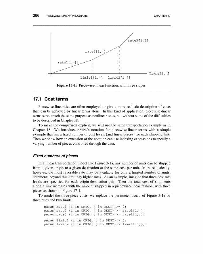
Figure 17-1: Piecewise-linear function, with three slopes.____________________________________________________________________________________________________________________________________________________________________________________________________________________________________________________________
17.1 Cost terms
Piecewise-linearities are often employed to give a more realistic description of coststhan can be achieved by linear terms alone. In this kind of application, piecewise-linearterms serve much the same purpose as nonlinear ones, but without some of the difficultiesto be described in Chapter 18.
To make the comparison explicit, we will use the same transportation example as inChapter 18. We introduce AMPL’s notation for piecewise-linear terms with a simpleexample that has a fixed number of cost levels (and linear pieces) for each shipping link.Then we show how an extension of the notation can use indexing expressions to specify avarying number of pieces controlled through the data.
Fixed numbers of pieces
In a linear transportation model like Figure 3-1a, any number of units can be shippedfrom a given origin to a given destination at the same cost per unit. More realistically,however, the most favorable rate may be available for only a limited number of units;shipments beyond this limit pay higher rates. As an example, imagine that three cost ratelevels are specified for each origin-destination pair. Then the total cost of shipmentsalong a link increases with the amount shipped in a piecewise-linear fashion, with threepieces as shown in Figure 17-1.
To model the three-piece costs, we replace the parameter cost of Figure 3-1a bythree rates and two limits:
param rate1 {i in ORIG, j in DEST} >= 0;param rate2 {i in ORIG, j in DEST} >= rate1[i,j];param rate3 {i in ORIG, j in DEST} >= rate2[i,j];
param limit1 {i in ORIG, j in DEST} > 0;param limit2 {i in ORIG, j in DEST} > limit1[i,j];
SECTION 17.1 COST TERMS 367
Shipments from i to j are charged at rate1[i,j] per unit up to limit1[i,j]units, then at rate2[i,j] per unit up to limit2[i,j], and then at rate3[i,j].Normally rate2[i,j] would be greater than rate1[i,j] and rate3[i,j] wouldbe greater than rate2[i,j], but they may be equal if the link from i to j does nothave three distinct rates.
In the linear transportation model, the objective is expressed in terms of the variablesand the parameter cost as follows:
var Trans {ORIG,DEST} >= 0;
minimize Total_Cost:sum {i in ORIG, j in DEST} cost[i,j] * Trans[i,j];
We could express a piecewise-linear objective analogously, by introducing three collec-tions of variables, one to represent the amount shipped at each rate:
var Trans1 {i in ORIG, j in DEST} >= 0, <= limit1[i,j];var Trans2 {i in ORIG, j in DEST} >= 0, <= limit2[i,j]
- limit1[i,j];var Trans3 {i in ORIG, j in DEST} >= 0;
minimize Total_Cost:sum {i in ORIG, j in DEST} (rate1[i,j] * Trans1[i,j]
But then the new variables would have to be introduced into all the constraints, and wewould also have to deal with these variables whenever we wanted to display the optimalresults. Rather than go to all this trouble, we would much prefer to describe thepiecewise-linear cost function explicitly in terms of the original variables. Since there isno standard way to describe piecewise-linear functions in algebraic notation, AMPL sup-plies its own syntax for this purpose.
The piecewise-linear function depicted in Figure 17-1 is written in AMPL as follows:
The expression between << and >> describes the piecewise-linear function, and is fol-lowed by the name of the variable to which it applies. (You can think of it as ‘‘multiply-ing’’ Trans[i,j], but by a series of coefficients rather than just one.) There are twoparts to the expression, a list of breakpoints where the slope of the function changes, anda list of the slopes — which in this case are the cost rates. The lists are separated by asemicolon, and members of each list are separated by commas. Since the first slopeapplies to values before the first breakpoint, and the last slope to values after the lastbreakpoint, the number of slopes must be one more than the number of breakpoints.
Although the lists of breakpoints and slopes are sufficient to describe the piecewise-linear cost function for optimization, they do not quite specify the function uniquely. Ifwe added, say, 10 to the cost at every point, we would have a different cost function eventhough all the breakpoints and slopes would be the same. To resolve this ambiguity,
subject to Supply {i in ORIG}:sum {j in DEST} Trans[i,j] = supply[i];
subject to Demand {j in DEST}:sum {i in ORIG} Trans[i,j] = demand[j];
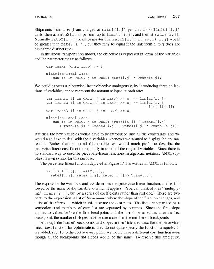
Figure 17-2: Piecewise-linear model with three slopes (transpl1.mod).____________________________________________________________________________________________________________________________________________________________________________________________________________________________________________________________
AMPL assumes that a piecewise-linear function evaluates to zero at zero, as in Figure17-1. Options for other possibilities are discussed later in this chapter.
Summing the cost over all links, the piecewise-linear objective function is now writ-ten
The declarations of the variables and constraints stay the same as before; the completemodel is shown in Figure 17-2.
Varying numbers of pieces
The approach taken in the preceding example is most useful when there are only a fewlinear pieces for each term. If there were, for example, 12 pieces instead of three, amodel defining rate1[i,j] through rate12[i,j] and limit1[i,j] throughlimit11[i,j] would be unwieldy. Realistically, moreover, there would more likelybe up to 12 pieces, rather than exactly 12, for each term; a term with fewer than 12 piecescould be handled by making some rates equal, but for large numbers of pieces this would
SECTION 17.2 COMMON TWO-PIECE AND THREE-PIECE TERMS 369
be a cumbersome device that would require many unnecessary data values and wouldobscure the actual number of pieces in each term.
A much better approach is to let the number of pieces (that is, the number of shippingrates) itself be a parameter of the model, indexed over the links:
param npiece {ORIG,DEST} integer >= 1;
We can then index the rates and limits over all combinations of links and pieces:
param rate {i in ORIG, j in DEST, p in 1..npiece[i,j]}>= if p = 1 then 0 else rate[i,j,p-1];
param limit {i in ORIG, j in DEST, p in 1..npiece[i,j]-1}> if p = 1 then 0 else limit[i,j,p-1];
For any particular origin i and destination j, the number of linear pieces in the cost termis given by npiece[i,j]. The slopes are rate[i,j,p] for p ranging from 1 tonpiece[i,j], and the intervening breakpoints are limit[i,j,p] for p from 1 tonpiece[i,j]-1. As before, there is one more slope than there are breakpoints.
To use AMPL’s piecewise-linear function notation with these data values, we have togive indexed lists of breakpoints and slopes, rather than the explicit lists of the previousexample. This is done by placing indexing expressions in front of the slope and break-point values:
minimize Total_Cost:sum {i in ORIG, j in DEST}
<<{p in 1..npiece[i,j]-1} limit[i,j,p];{p in 1..npiece[i,j]} rate[i,j,p]>> Trans[i,j];
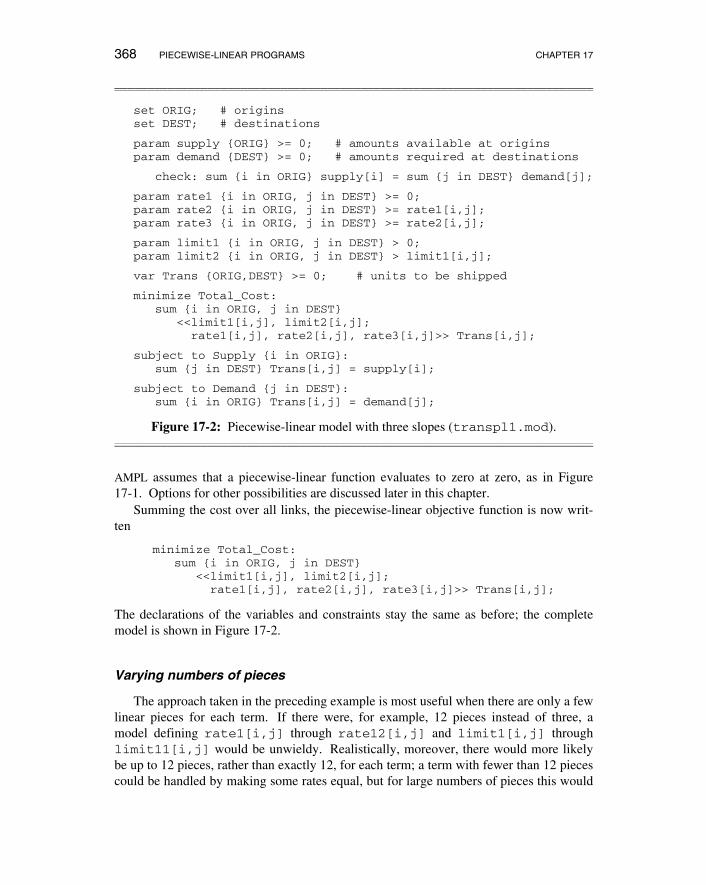
Once again, the rest of the model is the same. Figure 17-3a shows the whole model andFigure 17-3b illustrates how the data would be specified. Notice that sincenpiece["PITT","STL"] is 1, Trans["PITT","STL"] has only one slope andno breakpoints; this implies a one-piece linear term for Trans["PITT","STL"] inthe objective function.
17.2 Common two-piece and three-piece terms
Simple piecewise-linear terms have a variety of uses in otherwise linear models. Inthis section we present three cases: allowing limited violations of the constraints, analyz-ing infeasibility, and representing costs for variables that are meaningful at negative aswell as positive levels.
Penalty terms for ‘‘soft’’ constraints
Linear programs most easily express ‘‘hard’’ constraints: that production must be atleast at a certain level, for example, or that resources used must not exceed those avail-able. Real situations are often not nearly so definite. Production and resource use may
param supply {ORIG} >= 0; # amounts available at originsparam demand {DEST} >= 0; # amounts required at destinations
check: sum {i in ORIG} supply[i] = sum {j in DEST} demand[j];
param npiece {ORIG,DEST} integer >= 1;
param rate {i in ORIG, j in DEST, p in 1..npiece[i,j]}>= if p = 1 then 0 else rate[i,j,p-1];
param limit {i in ORIG, j in DEST, p in 1..npiece[i,j]-1}> if p = 1 then 0 else limit[i,j,p-1];
var Trans {ORIG,DEST} >= 0; # units to be shipped
minimize Total_Cost:sum {i in ORIG, j in DEST}
<<{p in 1..npiece[i,j]-1} limit[i,j,p];{p in 1..npiece[i,j]} rate[i,j,p]>> Trans[i,j];
subject to Supply {i in ORIG}:sum {j in DEST} Trans[i,j] = supply[i];
subject to Demand {j in DEST}:sum {i in ORIG} Trans[i,j] = demand[j];
Figure 17-3a: Piecewise-linear model with indexed slopes (transpl2.mod).____________________________________________________________________________________________________________________________________________________________________________________________________________________________________________________________
have certain preferred levels, yet we may be allowed to violate these levels by acceptingsome extra costs or reduced profits. The resulting ‘‘soft’’ constraints can be modeled byadding piecewise-linear ‘‘penalty’’ terms to the objective function.
For an example, we return to the multi-week production model developed in Chapter4. As seen in Figure 4-4, the constraints say that, in each of weeks 1 through T, totalhours used to make all products may not exceed hours available:
subject to Time {t in 1..T}:sum {p in PROD} (1/rate[p]) * Make[p,t] <= avail[t];
Suppose that, in reality, a larger number of hours may be used in each week, but at somepenalty per hour to the total profit. Specifically, we replace the parameter avail[t] bytwo availability levels and an hourly penalty rate:
Up to avail_min[t] hours are available without penalty in week t, and up toavail_max[t] hours are available at a loss of time_penalty[t] in profit for eachhour above avail_min[t].
To model this situation, we introduce a new variable Use[t] to represent the hoursused by production. Clearly Use[t] may not be less than zero, or greater than
SECTION 17.2 COMMON TWO-PIECE AND THREE-PIECE TERMS 371
param limit :=[GARY,*,*] FRA 1 500 FRA 2 1000 DET 1 500 DET 2 1000
LAN 1 500 LAN 2 1000 WIN 1 1000STL 1 500 STL 2 1000 FRE 1 1000LAF 1 500 LAF 2 1000
[CLEV,*,*] FRA 1 500 FRA 2 1000 DET 1 500 DET 2 1000LAN 1 500 LAN 2 1000 WIN 1 500 WIN 2 1000STL 1 500 STL 2 1000 FRE 1 500 FRE 2 1000LAF 1 500 LAF 2 1000
[PITT,*,*] FRA 1 1000 DET 1 1000 LAN 1 1000 WIN 1 1000FRE 1 1000 ;
Figure 17-3b: Data for piecewise-linear model (transpl2.dat).____________________________________________________________________________________________________________________________________________________________________________________________________________________________________________________________
avail_max[t]. In place of our previous constraint, we say that the total hours used tomake all products must equal Use[t]:
var Use {t in 1..T} >= 0, <= avail_max[t];
subject to Time {t in 1..T}:sum {p in PROD} (1/rate[p]) * Make[p,t] = Use[t];
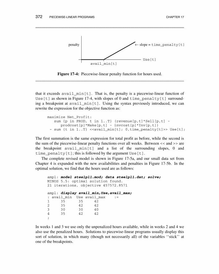
We can now describe the hourly penalty in terms of this new variable. If Use[t] isbetween 0 and avail_min[t], there is no penalty; if Use[t] is betweenavail_min[t] and avail_max[t], the penalty is time_penalty[t] per hour
Figure 17-4: Piecewise-linear penalty function for hours used.____________________________________________________________________________________________________________________________________________________________________________________________________________________________________________________________
that it exceeds avail_min[t]. That is, the penalty is a piecewise-linear function ofUse[t] as shown in Figure 17-4, with slopes of 0 and time_penalty[t] surround-ing a breakpoint at avail_min[t]. Using the syntax previously introduced, we canrewrite the expression for the objective function as:
maximize Net_Profit:sum {p in PROD, t in 1..T} (revenue[p,t]*Sell[p,t] -
prodcost[p]*Make[p,t] - invcost[p]*Inv[p,t])- sum {t in 1..T} <<avail_min[t]; 0,time_penalty[t]>> Use[t];
The first summation is the same expression for total profit as before, while the second isthe sum of the piecewise-linear penalty functions over all weeks. Between << and >> arethe breakpoint avail_min[t] and a list of the surrounding slopes, 0 andtime_penalty[t]; this is followed by the argument Use[t].
The complete revised model is shown in Figure 17-5a, and our small data set fromChapter 4 is expanded with the new availabilities and penalties in Figure 17-5b. In theoptimal solution, we find that the hours used are as follows:
ampl: model steelpl1.mod; data steelpl1.dat; solve;MINOS 5.5: optimal solution found.21 iterations, objective 457572.8571
In weeks 1 and 3 we use only the unpenalized hours available, while in weeks 2 and 4 wealso use the penalized hours. Solutions to piecewise-linear programs usually display thissort of solution, in which many (though not necessarily all) of the variables ‘‘stick’’ atone of the breakpoints.
SECTION 17.2 COMMON TWO-PIECE AND THREE-PIECE TERMS 373
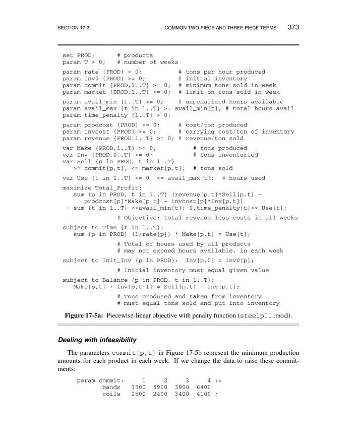
var Make {PROD,1..T} >= 0; # tons producedvar Inv {PROD,0..T} >= 0; # tons inventoriedvar Sell {p in PROD, t in 1..T}
>= commit[p,t], <= market[p,t]; # tons sold
var Use {t in 1..T} >= 0, <= avail_max[t]; # hours used
maximize Total_Profit:sum {p in PROD, t in 1..T} (revenue[p,t]*Sell[p,t] -
prodcost[p]*Make[p,t] - invcost[p]*Inv[p,t])- sum {t in 1..T} <<avail_min[t]; 0,time_penalty[t]>> Use[t];
# Objective: total revenue less costs in all weeks
subject to Time {t in 1..T}:sum {p in PROD} (1/rate[p]) * Make[p,t] = Use[t];
# Total of hours used by all products# may not exceed hours available, in each week
subject to Init_Inv {p in PROD}: Inv[p,0] = inv0[p];
# Initial inventory must equal given value
subject to Balance {p in PROD, t in 1..T}:Make[p,t] + Inv[p,t-1] = Sell[p,t] + Inv[p,t];
# Tons produced and taken from inventory# must equal tons sold and put into inventory
Figure 17-5a: Piecewise-linear objective with penalty function (steelpl1.mod).____________________________________________________________________________________________________________________________________________________________________________________________________________________________________________________________
Dealing with infeasibility
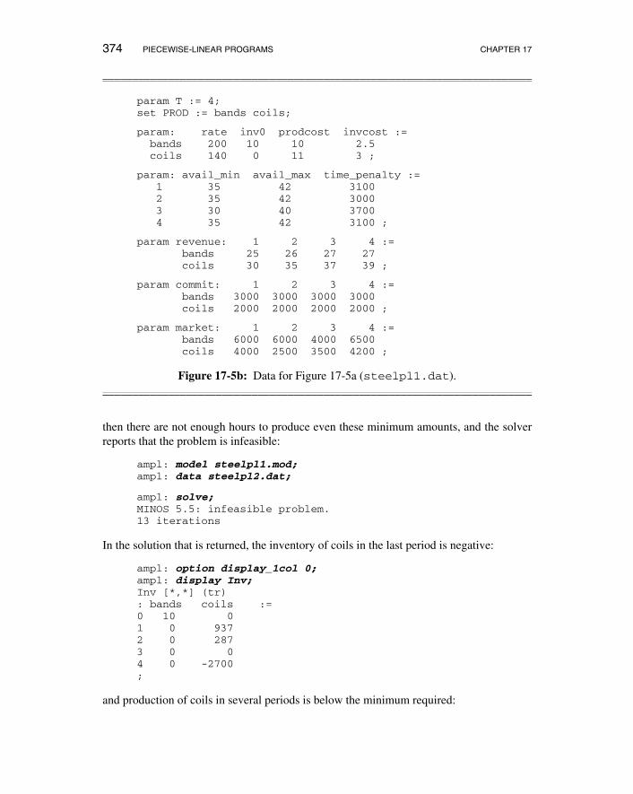
The parameters commit[p,t] in Figure 17-5b represent the minimum productionamounts for each product in each week. If we change the data to raise these commit-ments:
Figure 17-5b: Data for Figure 17-5a (steelpl1.dat).____________________________________________________________________________________________________________________________________________________________________________________________________________________________________________________________
then there are not enough hours to produce even these minimum amounts, and the solverreports that the problem is infeasible:
Figure 17-6: Penalty function for hours used, with two breakpoints.____________________________________________________________________________________________________________________________________________________________________________________________________________________________________________________________
These are typical of the infeasible results that solvers return. The infeasibilities are scat-tered around the solution, so that it is hard to tell what changes might be necessary toachieve feasibility. By extending the idea of penalties, we can better concentrate theinfeasibility where it can be understood.
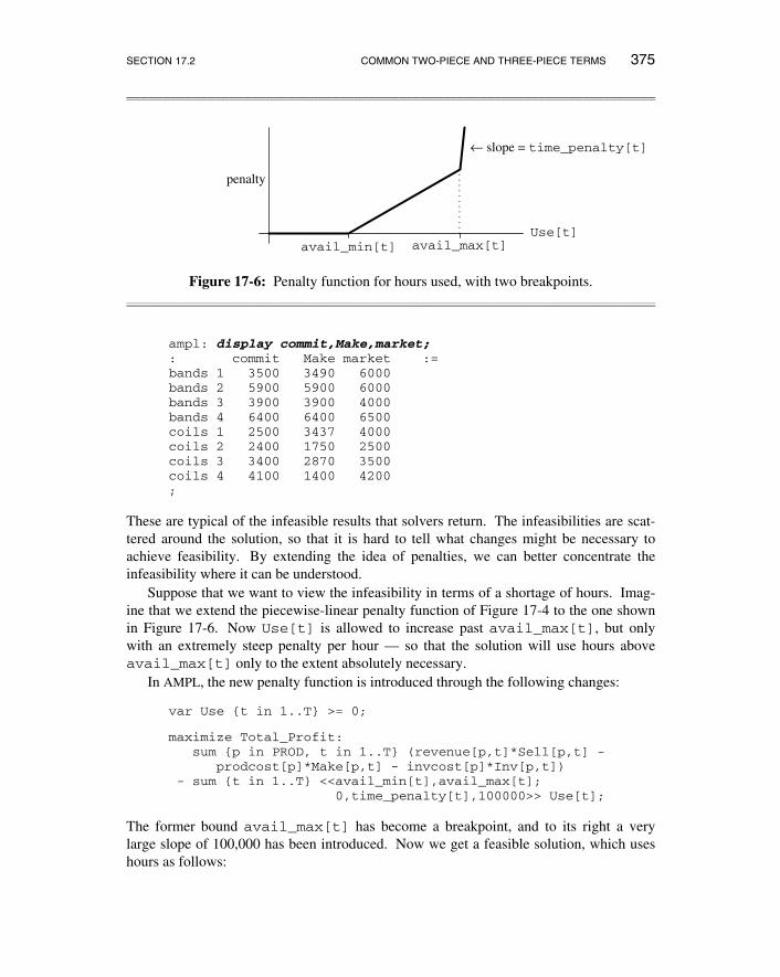
Suppose that we want to view the infeasibility in terms of a shortage of hours. Imag-ine that we extend the piecewise-linear penalty function of Figure 17-4 to the one shownin Figure 17-6. Now Use[t] is allowed to increase past avail_max[t], but onlywith an extremely steep penalty per hour — so that the solution will use hours aboveavail_max[t] only to the extent absolutely necessary.
In AMPL, the new penalty function is introduced through the following changes:
var Use {t in 1..T} >= 0;
maximize Total_Profit:sum {p in PROD, t in 1..T} (revenue[p,t]*Sell[p,t] -
prodcost[p]*Make[p,t] - invcost[p]*Inv[p,t])- sum {t in 1..T} <<avail_min[t],avail_max[t];
0,time_penalty[t],100000>> Use[t];
The former bound avail_max[t] has become a breakpoint, and to its right a verylarge slope of 100,000 has been introduced. Now we get a feasible solution, which useshours as follows:
Figure 17-7: Penalty function for sales.____________________________________________________________________________________________________________________________________________________________________________________________________________________________________________________________
ampl: model steelpl2.mod; data steelpl2.dat; solve;MINOS 5.5: optimal solution found.19 iterations, objective -1576814.857
This table implies that the commitments can be met only by adding about 21 hours,mostly in the last week.
Alternatively, we may view the infeasibility in terms of an excess of commitments.For this purpose we subtract a very large penalty from the objective for each unit thatSell[p,t] falls below commit[p,t]; the penalty as a function of Sell[p,t] isdepicted in Figure 17-7.
Since this function has a breakpoint at commit[p,t], with a slope of 0 to the rightand a very negative value to the left, it would seem that the AMPL representation could be
<<commit[p,t]; -100000,0>> Sell[p,t]
Recall, however, AMPL’s convention that such a function takes the value zero at zero.Figure 17-7 clearly shows that we want our penalty function to take a positive value atzero, so that it will fall to zero at commit[p,t] and beyond. In fact we want the func-tion to take a value of 100000 * commit[p,t] at zero, and we could express thefunction properly by adding this constant to the penalty expression:
The same thing may be said more concisely by using a second argument that statesexplicitly where the piecewise-linear function should evaluate to zero:
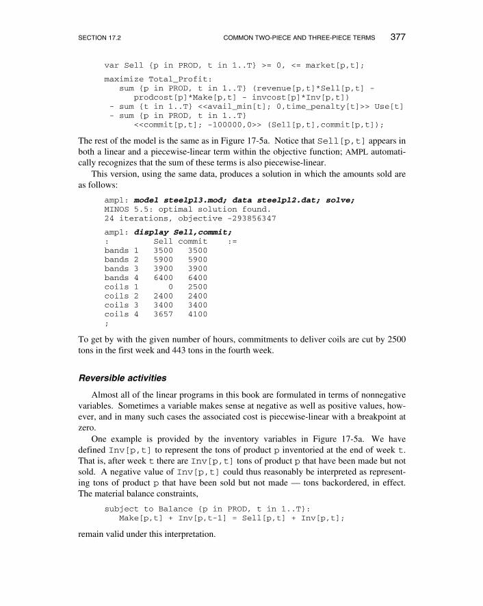
The rest of the model is the same as in Figure 17-5a. Notice that Sell[p,t] appears inboth a linear and a piecewise-linear term within the objective function; AMPL automati-cally recognizes that the sum of these terms is also piecewise-linear.
This version, using the same data, produces a solution in which the amounts sold areas follows:
ampl: model steelpl3.mod; data steelpl2.dat; solve;MINOS 5.5: optimal solution found.24 iterations, objective -293856347
To get by with the given number of hours, commitments to deliver coils are cut by 2500tons in the first week and 443 tons in the fourth week.
Reversible activities
Almost all of the linear programs in this book are formulated in terms of nonnegativevariables. Sometimes a variable makes sense at negative as well as positive values, how-ever, and in many such cases the associated cost is piecewise-linear with a breakpoint atzero.
One example is provided by the inventory variables in Figure 17-5a. We havedefined Inv[p,t] to represent the tons of product p inventoried at the end of week t.That is, after week t there are Inv[p,t] tons of product p that have been made but notsold. A negative value of Inv[p,t] could thus reasonably be interpreted as represent-ing tons of product p that have been sold but not made — tons backordered, in effect.The material balance constraints,
subject to Balance {p in PROD, t in 1..T}:Make[p,t] + Inv[p,t-1] = Sell[p,t] + Inv[p,t];
remain valid under this interpretation.
378 PIECEWISE-LINEAR PROGRAMS CHAPTER 17
This analysis suggests that we remove the >= 0 from the declaration of Inv in ourmodel. Then backordering might be especially attractive if the sales price were expectedto drop in later weeks, like this:
The source of difficulty is in the objective function, where invcost[p] * Inv[p,t]is subtracted from the sales revenue. When Inv[p,t] is negative, a negative amount issubtracted, increasing the apparent total profit. The greater the amount backordered, themore the total profit is increased — hence the odd solution in which the maximum possi-ble sales are backordered, while nothing is produced!
A proper inventory cost function for this model looks like the one graphed in Figure17-8. It increases both as Inv[p,t] becomes more positive (greater inventories) and asInv[p,t] becomes more negative (greater backorders). We represent this piecewise-linear function in AMPL by declaring a backorder cost to go with the inventory cost:____________________________________________________________________________________________________________________________________________________________________________________________________________________________________________________________
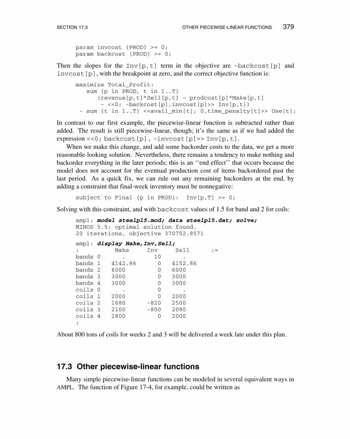
Then the slopes for the Inv[p,t] term in the objective are -backcost[p] andinvcost[p], with the breakpoint at zero, and the correct objective function is:
- sum {t in 1..T} <<avail_min[t]; 0,time_penalty[t]>> Use[t];
In contrast to our first example, the piecewise-linear function is subtracted rather thanadded. The result is still piecewise-linear, though; it’s the same as if we had added theexpression <<0; backcost[p], -invcost[p]>> Inv[p,t].
When we make this change, and add some backorder costs to the data, we get a morereasonable-looking solution. Nevertheless, there remains a tendency to make nothing andbackorder everything in the later periods; this is an ‘‘end effect’’ that occurs because themodel does not account for the eventual production cost of items backordered past thelast period. As a quick fix, we can rule out any remaining backorders at the end, byadding a constraint that final-week inventory must be nonnegative:
subject to Final {p in PROD}: Inv[p,T] >= 0;
Solving with this constraint, and with backcost values of 1.5 for band and 2 for coils:
ampl: model steelpl5.mod; data steelpl5.dat; solve;MINOS 5.5: optimal solution found.20 iterations, objective 370752.8571
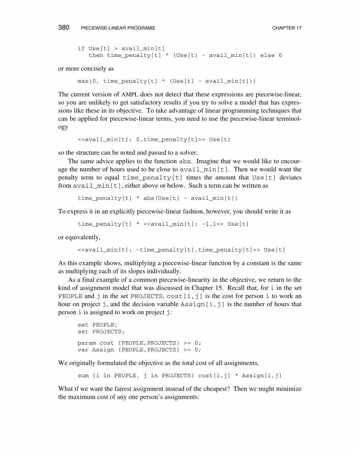
The current version of AMPL does not detect that these expressions are piecewise-linear,so you are unlikely to get satisfactory results if you try to solve a model that has expres-sions like these in its objective. To take advantage of linear programming techniques thatcan be applied for piecewise-linear terms, you need to use the piecewise-linear terminol-ogy
<<avail_min[t]; 0,time_penalty[t]>> Use[t]
so the structure can be noted and passed to a solver.The same advice applies to the function abs. Imagine that we would like to encour-
age the number of hours used to be close to avail_min[t]. Then we would want thepenalty term to equal time_penalty[t] times the amount that Use[t] deviatesfrom avail_min[t], either above or below. Such a term can be written as
time_penalty[t] * abs(Use[t] - avail_min[t])
To express it in an explicitly piecewise-linear fashion, however, you should write it as
As this example shows, multiplying a piecewise-linear function by a constant is the sameas multiplying each of its slopes individually.
As a final example of a common piecewise-linearity in the objective, we return to thekind of assignment model that was discussed in Chapter 15. Recall that, for i in the setPEOPLE and j in the set PROJECTS, cost[i,j] is the cost for person i to work anhour on project j, and the decision variable Assign[i,j] is the number of hours thatperson i is assigned to work on project j:
param supply {PEOPLE} >= 0; # hours each person is availableparam demand {PROJECTS} >= 0; # hours each project requires
check: sum {i in PEOPLE} supply[i]= sum {j in PROJECTS} demand[j];
param cost {PEOPLE,PROJECTS} >= 0; # cost per hour of workparam limit {PEOPLE,PROJECTS} >= 0; # maximum contributions
# to projects
var M;var Assign {i in PEOPLE, j in PROJECTS} >= 0, <= limit[i,j];
minimize Max_Cost: M;
subject to M_def {i in PEOPLE}:M >= sum {j in PROJECTS} cost[i,j] * Assign[i,j];
subject to Supply {i in PEOPLE}:sum {j in PROJECTS} Assign[i,j] = supply[i];
subject to Demand {j in PROJECTS}:sum {i in PEOPLE} Assign[i,j] = demand[j];
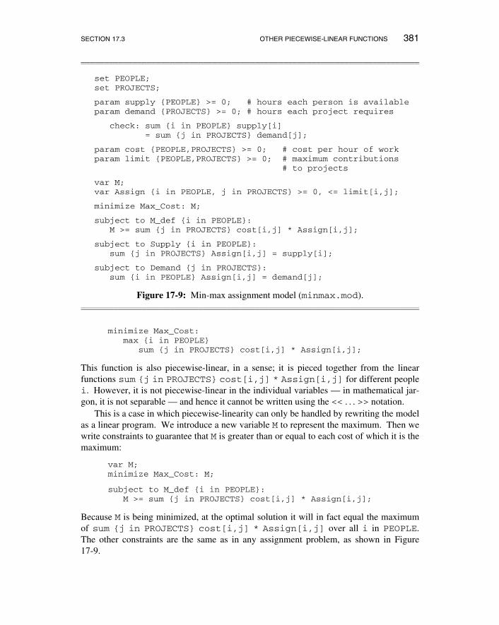
Figure 17-9: Min-max assignment model (minmax.mod).____________________________________________________________________________________________________________________________________________________________________________________________________________________________________________________________
minimize Max_Cost:max {i in PEOPLE}
sum {j in PROJECTS} cost[i,j] * Assign[i,j];
This function is also piecewise-linear, in a sense; it is pieced together from the linearfunctions sum {j in PROJECTS} cost[i,j] * Assign[i,j] for different peoplei. However, it is not piecewise-linear in the individual variables — in mathematical jar-gon, it is not separable — and hence it cannot be written using the << . . . >> notation.
This is a case in which piecewise-linearity can only be handled by rewriting the modelas a linear program. We introduce a new variable M to represent the maximum. Then wewrite constraints to guarantee that M is greater than or equal to each cost of which it is themaximum:
var M;minimize Max_Cost: M;
subject to M_def {i in PEOPLE}:M >= sum {j in PROJECTS} cost[i,j] * Assign[i,j];
Because M is being minimized, at the optimal solution it will in fact equal the maximumof sum {j in PROJECTS} cost[i,j] * Assign[i,j] over all i in PEOPLE.The other constraints are the same as in any assignment problem, as shown in Figure17-9.
382 PIECEWISE-LINEAR PROGRAMS CHAPTER 17
This kind of reformulation can be applied to any problem that has a ‘‘min-max’’objective. The same idea works for the analogous ‘‘max-min’’ objective, withmaximize instead of minimize and with M <= . . . in the constraints.
17.4 Guidelines for piecewise-linear optimization
AMPL’s piecewise-linear notation has the power to specify a variety of useful func-tions. We summarize below its various forms, most of which have been illustrated earlierin this chapter.
Because this notation is so general, it can be used to specify many functions that arenot readily optimized by any efficient and reliable algorithms. We conclude by describ-ing the kinds of piecewise-linear functions that are most likely to appear in tractable mod-els, with particular emphasis on the property of convexity or concavity.
Forms for piecewise-linear expressions
An AMPL piecewise-linear term has the general form
<<breakpoint - list; slope - list>> pl - argument
where breakpoint-list and slope-list each consist of a comma-separated list of one or moreitems. An item may be an individual arithmetic expression, or an indexing expressionfollowed by an arithmetic expression. In the latter case, the indexing expression must bean ordered set; the item is expanded to a list by evaluating the arithmetic expression oncefor each set member (as in the example of Figure 17-3a).
After any indexed items are expanded, the number of slopes must be one more thanthe number of breakpoints, and the breakpoints must be nondecreasing. The resultingpiecewise-linear function is constructed by interleaving the slopes and breakpoints in theorder given, with the first slope to the left of the first breakpoint, and the last slope to theright of the last breakpoint. By indexing breakpoints over an empty set, it is possible tospecify no breakpoints and one slope, in which case the function is linear.
The pl-argument may have one of the forms
var - ref(arg - expr)(arg - expr, zero - expr)
The var-ref (a reference to a previously declared variable) or the arg-expr (an arithmeticexpression) specifies the point where the piecewise-linear function is to be evaluated.The zero-expr is an arithmetic expression that specifies a place where the function is zero;when the zero-expr is omitted, the function is assumed to be zero at zero.
SECTION 17.4 GUIDELINES FOR PIECEWISE-LINEAR OPTIMIZATION 383
Suggestions for piecewise-linear models
As seen in all of our examples, AMPL’s terminology for piecewise-linear functions ofvariables is limited to describing functions of individual variables. In model declarations,no variables may appear in the breakpoint-list, slope-list and zero-expr (if any), while anarg-expr can only be a reference to an individual variable. (Piecewise-linear expressionsin commands like display may use variables without limitation, however.)
A piecewise-linear function of an individual variable remains such a function whenmultiplied or divided by an arithmetic expression without variables. AMPL also treats asum or difference of piecewise-linear and linear functions of the same variable as repre-senting one piecewise-linear function of that variable. A separable piecewise-linearfunction of a model’s variables is a sum or difference (using +, - or sum) of piecewise-linear or linear functions of the individual variables. Optimizers can effectively handlethese separable functions, which are the ones that appear in our examples.
A piecewise-linear function is convex if successive slopes are nondecreasing (alongwith the breakpoints), and is concave if the slopes are nonincreasing. The two kinds ofpiecewise-linear optimization most easily handled by solvers are minimizing a separableconvex piecewise-linear function, and maximizing a separable concave piecewise-linearfunction, subject to linear constraints. You can easily check that all of this chapter’sexamples are of these kinds. AMPL can obtain solutions in these cases by translating toan equivalent linear program, applying any LP solver, and then translating the solutionback; the whole sequence occurs automatically when you type solve.
Outside of these two cases, optimizing a separable piecewise-linear function must beviewed as an application of integer programming — the topic of Chapter 20 — andAMPL must translate piecewise-linear terms to equivalent integer programming forms.This, too, is done automatically, for solution by an appropriate solver. Because integerprograms are usually much harder to solve than similar linear programs of comparablesize, however, you should not assume that just any separable piecewise-linear functioncan be readily optimized; a degree of experimentation may be necessary to determinehow large an instance your solver can handle. The best results are likely to be obtainedby solvers that accept an option known (mysteriously) as ‘‘special ordered sets of type2’’; check the solver-specific documentation for details.
The situation for the constraints can be described in a similar way. However, a sepa-rable piecewise-linear function in a constraint can be handled through linear program-ming only under a restrictive set of circumstances:
• If it is convex and on the left-hand side of a ≤ constraint (or equivalently, theright-hand side of a ≥ constraint);
• If it is concave and on the left-hand side of a ≥ constraint (or equivalently, theright-hand side of a ≤ constraint).
Other piecewise-linearities in the constraints must be dealt with through integer program-ming techniques, and the preceding comments for the case of the objective apply.
If you have access to a solver that can handle piecewise-linearities directly, you canturn off AMPL’s translation to the linear or integer programming form by setting the
384 PIECEWISE-LINEAR PROGRAMS CHAPTER 17
option pl_linearize to 0. The case of minimizing a convex or maximizing a con-cave separable piecewise-linear function can in particular be handled very efficiently bypiecewise-linear generalizations of LP techniques. A solver intended for nonlinear pro-gramming may also accept piecewise-linear functions, but it is unlikely to handle themreliably unless it has been specially designed for ‘‘nondifferentiable’’ optimization.
The differences between hard and easy piecewise-linear cases can be slight. Thischapter’s transportation example is easy, in particular because the shipping rates increasealong with shipping volume. The same example would be hard if economies of scalecaused shipping rates to decrease with volume, since then we would be minimizing a con-cave rather than a convex function. We cannot say definitively that shipping rates oughtto be one way or the other; their behavior depends upon the specifics of the situationbeing modeled.
In all cases, the difficulty of piecewise-linear optimization gradually increases withthe total number of pieces. Thus piecewise-linear cost functions are most effective whenthe costs can be described or approximated by relatively few pieces. If you need morethan about a dozen pieces to describe a cost accurately, you may be better off using anonlinear function as described in Chapter 18.
Bibliography
Robert Fourer, ‘‘A Simplex Algorithm for Piecewise-Linear Programming III: ComputationalAnalysis and Applications.’’ Mathematical Programming 53 (1992) pp. 213–235. A survey ofconversions from piecewise-linear to linear programs, and of applications.
Robert Fourer and Roy E. Marsten, ‘‘Solving Piecewise-Linear Programs: Experiments with aSimplex Approach.’’ ORSA Journal on Computing 4 (1992) pp. 16–31. Descriptions of variedapplications and of experience in solving them.
Spyros Kontogiorgis, ‘‘Practical Piecewise-Linear Approximation for Monotropic Optimization.’’INFORMS Journal on Computing 12 (2000) pp. 324–340. Guidelines for choosing the breakpointswhen approximating a nonlinear function by a piecewise-linear one.
Exercises
17-1. Piecewise-linear models are sometimes an alternative to the nonlinear models described inChapter 18, replacing a smooth curve by a series of straight-line segments. This exercise dealswith the model shown in Figure 18-4.
(a) Reformulate the model of Figure 18-4 so that it approximates each nonlinear term
Trans[i,j] / (1 - Trans[i,j]/limit[i,j])
by a piecewise-linear term having three pieces. Set the breakpoints at (1/3) * limit[i,j]and (2/3) * limit[i,j]. Pick the slopes so that the approximation equals the original nonlin-ear term when Trans[i,j] is 0, 1/3 * limit[i,j], 2/3 * limit[i,j], or 11/12 *limit[i,j]; you should find that the three slopes are 3/2, 9/2 and 36 in every term, regardless
SECTION 17.4 GUIDELINES FOR PIECEWISE-LINEAR OPTIMIZATION 385
of the size of limit[i,j]. Finally, place an explicit upper limit of 0.99 * limit[i,j] onTrans[i,j].
(b) Solve the approximation with the data given in Figure 18-5, and compare the optimal shipmentamounts to the amounts recommended by the nonlinear model.
(c) Formulate a more sophisticated version in which the number of linear pieces for each term isgiven by a parameter nsl. Pick the breakpoints to be at (k/nsl) * limit[i,j] for k from 1to nsl-1. Pick the slopes so that the piecewise-linear function equals the original nonlinear func-tion when Trans[i,j] is (k/nsl) * limit[i,j] for any k from 0 to nsl-1, or whenTrans[i,j] is (nsl-1/4)/nsl * limit[i,j].
Check your model by showing that you get the same results as in (b) when nsl is 3. Then, by try-ing higher values of nsl, determine how many linear pieces the approximation requires in order todetermine all shipment amounts to within about 10% of the amounts recommended by the originalnonlinear model.
17-2. This exercise asks how you might convert the demand constraints in the transportationmodel of Figure 3-1a into the kind of ‘‘soft’’ constraints described in Section 17.2.
Suppose that instead of a single parameter called demand[j] at each destination j, you are giventhe following four parameters that describe a more complicated situation:
dem_min_abs[j] absolute minimum that must be shipped to jdem_min_ask[j] preferred minimum amount shipped to jdem_max_ask[j] preferred maximum amount shipped to jdem_max_abs[j] absolute maximum that may be shipped to j
There are also two penalty costs for shipment amounts outside of the preferred limits:
dem_min_pen penalty per unit that shipments fall below dem_min_ask[j]dem_max_pen penalty per unit that shipments exceed dem_max_ask[j]
Because the total shipped to j is no longer fixed, a new variable Receive[j] is introduced torepresent the amount received at j.
(a) Modify the model of Figure 3-1a to use this new information. The modifications will involvedeclaring Receive[j] with the appropriate lower and upper bounds, adding a three-piecepiecewise-linear penalty term to the objective function, and substituting Receive[j] fordemand[j] in the constraints.
(b) Add the following demand information to the data of Figure 3-1b:
Let dem_min_pen and dem_max_pen be 2 and 4, respectively. Find the new optimal solution.In the solution, which destinations receive shipments that are outside the preferred levels?
17-3. When the diet model of Figure 2-1 is run with the data of Figure 2-3, there is no feasiblesolution. This exercise asks you to use the ideas of Section 17.2 to find some good near-feasiblesolutions.
386 PIECEWISE-LINEAR PROGRAMS CHAPTER 17
(a) Modify the model so that it is possible, at a very high penalty, to purchase more than the speci-fied maximum of a food. In the resulting solution, which maximums are exceeded?
(b) Modify the model so that it is possible, at a very high penalty, to supply more than the specifiedmaximum of a nutrient. In the resulting solution, which maximums are exceeded?
(c) Using extremely large penalties, such as 1020 may give the solver numerical difficulties.Experiment to see how available solvers behave when you use penalty terms like 1020 and 1030.
17-4. In the model of Exercise 4-4(b), the change in crews from one period to the next is limitedto some number M. As an alternative to imposing this limit, suppose that we introduce a new vari-able D t that represents the change in number of crews (in all shifts) at period t. This variable maybe positive, indicating an increase in crews over the previous period, or negative, indicating adecrease in crews.
To make use of this variable, we introduce a defining constraint,
D t = Σ s ∈S(Y st − Y s ,t − 1 ),
for each t = 1, . . . , T. We then estimate costs of c + per crew added from period to period, and c −
per crew dropped from period to period; as a result, the following cost must be included in theobjective for each month t:
c − D t , if D t < 0;
c + D t , if D t > 0.
Reformulate the model in AMPL accordingly, using a piecewise-linear function to represent thisextra cost.
Solve using c − = –20000 and c + = 100000, together with the data previously given. How does thissolution compare to the one from Exercise 4-4(b)?
17-5. The following ‘‘credit scoring’’ problem appears in many contexts, including the process-ing of credit card applications. A set APPL of people apply for a card, each answering a set QUESof questions on the application. The response of person i to question j is converted to a number,ans[i,j]; typical numbers are years at current address, monthly income, and a home ownershipindicator (say, 1 if a home is owned and 0 otherwise).
To summarize the responses, the card issuer chooses weights Wt[j], from which a score for eachperson i in APPL is computed by the linear formula
sum {j in QUES} ans[i,j] * Wt[j]
The issuer also chooses a cutoff, Cut; credit is granted when an applicant’s score is greater than orequal to the cutoff, and is denied when the score is less than the cutoff. In this way the decisioncan be made objectively (if not always most wisely).
To choose the weights and the cutoff, the card issuer collects a sample of previously acceptedapplications, some from people who turned out to be good customers, and some from people whonever paid their bills. If we denote these two collections of people by sets GOOD and BAD, then theideal weights and cutoff (for this data) would satisfy
sum {j in QUES} ans[i,j] * Wt[j] >= Cut for each i in GOODsum {j in QUES} ans[i,j] * Wt[j] < Cut for each i in BAD
Since the relationship between answers to an application and creditworthiness is imprecise at best,however, no values of Wt[j] and Cut can be found to satisfy all of these inequalities. Instead,
SECTION 17.4 GUIDELINES FOR PIECEWISE-LINEAR OPTIMIZATION 387
the issuer has to choose values that are merely the best possible, in some sense. There are anynumber of ways to make such a choice; here, naturally, we consider an optimization approach.
(a) Suppose that we define a new variable Diff[i] that equals the difference between person i’sscore and the cutoff:
Diff[i] = sum {j in QUES} ans[i,j] * Wt[j] - Cut
Clearly the undesirable cases are where Diff[i] is negative for i in GOOD, and where it is non-negative for i in BAD. To discourage these cases, we can tell the issuer to minimize the function
sum {i in GOOD} max(0,-Diff[i]) + sum {i in BAD} max(0,Diff[i])
Explain why minimizing this function tends to produce a desirable choice of weights and cutoff.
(b) The expression above is a piecewise-linear function of the variables Diff[i]. Rewrite itusing AMPL’s notation for piecewise-linear functions.
(c) Incorporate the expression from (b) into an AMPL model for finding the weights and cutoff.
(d) Given this approach, any positive value for Cut is as good as any other. We can fix it at a con-venient round number — say, 100. Explain why this is the case.
(e) Using a Cut of 100, apply the model to the following imaginary credit data:
set GOOD := _17 _18 _19 _22 _24 _26 _28 _29 ;set BAD := _15 _16 _20 _21 _23 _25 _27 _30 ;
What are the chosen weights? Using these weights, how many of the good customers would bedenied a card, and how many of the bad risks would be granted one?
You should find that a lot of the bad risks have scores right at the cutoff. Why does this happen inthe solution? How might you adjust the cutoff to deal with it?
(f) To force scores further away from the cutoff (in the desired direction), it might be preferable touse the following objective,
sum {i in GOOD} max(0,-Diff[i]+offset) +sum {i in BAD} max(0,Diff[i]+offset)
where offset is a positive parameter whose value is supplied. Explain why this change has thedesired effect. Try offset values of 2 and 10 and compare the results with those in (e).
388 PIECEWISE-LINEAR PROGRAMS CHAPTER 17
(g) Suppose that giving a card to a bad credit risk is considered much more undesirable than refus-ing a card to a good credit risk. How would you change the model to take this into account?
(h) Suppose that when someone’s application is accepted, his or her score is also used to suggest aninitial credit limit. Thus it is particularly important that bad credit risks not receive very largescores. How would you add pieces to the piecewise-linear objective function terms to account forthis concern?
17-6. In Exercise 18-3, we suggest a way to estimate position, velocity and acceleration valuesfrom imprecise data, by minimizing a nonlinear ‘‘sum of squares’’ function:
j = 1Σn
[h j − (a 0 − a 1 t j − 1⁄2 a 2 tj2 ) ]2.
An alternative approach instead minimizes a sum of absolute values:
j = 1Σn
h j − (a 0 − a 1 t j − 1⁄2 a 2 tj2 ) .
(a) Substitute the sum of absolute values directly for the sum of squares in the model from Exercise18-3, first with the abs function, and then with AMPL’s explicit piecewise-linear notation.
Explain why neither of these formulations is likely to be handled effectively by any solver.
(b) To model this situation effectively, we introduce variables e j to represent the individual formu-las h j − (a 0 − a 1 t j − 1⁄2 a 2 tj
2 ) whose absolute values are being taken. Then we can express theminimization of the sum of absolute values as the following constrained optimization problem:
Minimizej = 1Σn
e j
Subject to e j = h j − (a 0 − a 1 t j − 1⁄2 a 2 tj2 ), j = 1, . . . , n
Write an AMPL model for this formulation, using the piecewise-linear notation for the terms e j .
(c) Solve for a 0, a 1, and a 2 using the data from Exercise 18-3. How much difference is therebetween this estimate and the least-squares one?
Use display to print the e j values for both the least-squares and the least-absolute-values solu-tions. What is the most obvious qualitative difference?
(d) Yet another possibility is to focus on the greatest absolute deviation, rather than the sum:
j = 1 , . . . ,nmax h j − (a 0 − a 1 t j − 1⁄2 a 2 tj
2 ) .
Formulate an AMPL linear program that will minimize this quantity, and test it on the same data asbefore. Compare the resulting estimates and e j values. Which of the three estimates would youchoose in this case?
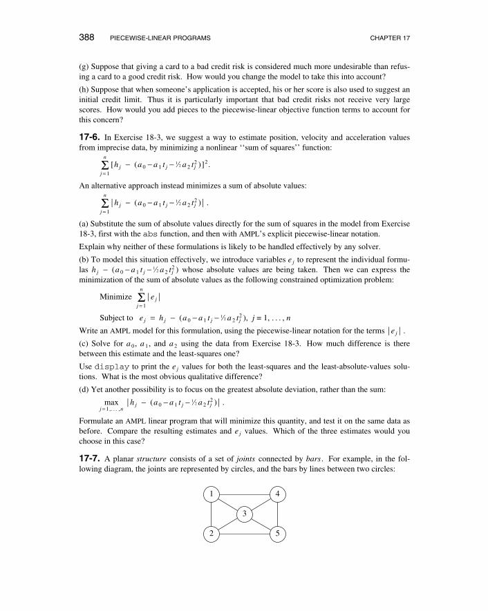
17-7. A planar structure consists of a set of joints connected by bars . For example, in the fol-lowing diagram, the joints are represented by circles, and the bars by lines between two circles:
1
2
3
4
5
SECTION 17.4 GUIDELINES FOR PIECEWISE-LINEAR OPTIMIZATION 389
Consider the problem of finding a minimum-weight structure to meet certain external forces. Welet J be the set of joints, and B⊆J×J be the set of admissible bars; for the diagram above, we couldtake J = { 1 , 2 , 3 , 4 , 5 }, and
The ‘‘origin’’ and ‘‘destination’’ of a bar are arbitrary. The bar between joints 1 and 2, for exam-ple, could be represented in B by either (1,2) or (2,1), but it need not be represented by both.
We can use two-dimensional Euclidean coordinates to specify the position of each joint in theplane, taking some arbitrary point as the origin:
aix horizontal position of joint i relative to the origin
aiy vertical position of joint i relative to the origin
For the example, if the origin lies exactly at joint 2, we might have
(a1x , a1
y ) = (0, 2), (a2x , a2
y ) = (0, 0), (a3x , a3
y ) = (2, 1),
(a4x , a4
y ) = (4, 2), (a5x , a5
y ) = (4, 0).
The remaining data consist of the external forces on the joints:
fix horizontal component of the external force on joint i
fiy vertical component of the external force on joint i
To resist this force, a subset S⊆J of joints is fixed in position. (It can be proved that fixing twojoints is sufficient to guarantee a solution.)
The external forces induce stresses on the bars, which we can represent as
F i j if > 0, tension on bar (i , j)
if < 0, compression of bar (i , j)
A set of stresses is in equilibrium if the external forces, tensions and compressions balance at alljoints, in both the horizontal and vertical components — except at the fixed joints. That is, foreach joint k ∉S,
Σ i ∈J: (i ,k) ∈Bcik
x F ik − Σ j ∈J: (k, j) ∈Bck j
x F k j = fkx
Σ i ∈J: (i ,k) ∈Bcik
y F ik − Σ j ∈J: (k, j) ∈Bck j
y F k j = fky,
where cstx and cst
y are the cosines of the direction from joint s to joint t with the horizontal and verti-cal axes,
cstx = (at
x − asx )/ l st ,
csty = (at
y − asy )/ l st ,
and l st is the length of the bar (s ,t):
l st = √ (atx − as
x )2 + (aty − as
y )2 .
In general, there are infinitely many different sets of equilibrium stresses. However, it can beshown that a given system of stresses will be realized in a structure of minimum weight if and onlyif the cross-sectional areas of the bars are proportional to the absolute values of the stresses. Sincethe weight of a bar is proportional to the cross section times length, we can take the (suitablyscaled) weight of bar (i , j) to be
w i j = l i j.F i j .
The problem is then to find a system of stresses F i j that meet the equilibrium conditions, and thatminimize the sum of the weights w i j over all bars (i , j) ∈B.
(a) The indexing sets for this linear program can be declared in AMPL as:
390 PIECEWISE-LINEAR PROGRAMS CHAPTER 17
set joints;set fixed within joints;set bars within {i in joints, j in joints: i <> j};
Using these set declarations, formulate an AMPL model for the minimum-weight structural designproblem. Use the piecewise-linear notation of this chapter to represent the absolute-value terms inthe objective function.
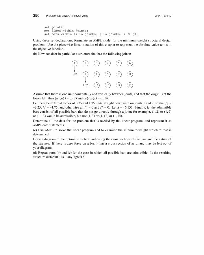
(b) Now consider in particular a structure that has the following joints:
1 2 3 4 5 6
3.25 7 8 9 10 11
1.75 12 13 14 15
Assume that there is one unit horizontally and vertically between joints, and that the origin is at thelower left; thus (a1
x ,a1y ) = (0, 2) and (a15
x ,a15y ) = (5, 0).
Let there be external forces of 3.25 and 1.75 units straight downward on joints 1 and 7, so that f1y =
–3.25, f7y = –1.75, and otherwise all fi
x = 0 and fiy = 0. Let S = {6,15}. Finally, let the admissible
bars consist of all possible bars that do not go directly through a joint; for example, (1, 2) or (1, 9)or (1, 13) would be admissible, but not (1, 3) or (1, 12) or (1, 14).
Determine all the data for the problem that is needed by the linear program, and represent it asAMPL data statements.
(c) Use AMPL to solve the linear program and to examine the minimum-weight structure that isdetermined.
Draw a diagram of the optimal structure, indicating the cross sections of the bars and the nature ofthe stresses. If there is zero force on a bar, it has a cross section of zero, and may be left out ofyour diagram.
(d) Repeat parts (b) and (c) for the case in which all possible bars are admissible. Is the resultingstructure different? Is it any lighter?