Page 1
1
Piecewise potential vorticity diagnosis of the
development of a polar low over the Sea of Japan
By Longtao Wu1*, Jonathan E. Martin1 and Grant W. Petty1
1Department of Atmospheric and Oceanic Sciences
University of Wisconsin-Madison, Madison, WI 53706, USA
____________________
*Corresponding author. E-mail: [email protected]
Page 2
2
Abstract
The piecewise potential vorticity (PV) inversion method developed by Davis and
Emanuel (1991) is used to diagnose the development processes of a polar low over the
Sea of Japan in December 2003. The synoptic scale balanced flows associated with the
polar low are successfully captured using the inversion method. It is shown that,
antecedent to the development of the polar low, a positive lower-tropospheric
temperature anomaly was induced by the approach of a positive tropopause-level PV
anomaly over the northern Sea of Japan. The analysis suggests that the polar low was
initiated as a result of the combined effect of the positive PV anomaly near the
tropopause and the near-surface positive temperature anomaly. The rapid height falls in
the lower troposphere were primarily contributed by the upper tropospheric PV anomaly.
Further intensification of the polar low was afforded by latent heat release associated
with cloud and precipitation processes. After the polar low moved over northern Honshu,
quick dissipation was primarily rendered by the thinning and elongating of the upper
level PV anomaly that led to a rapid reduction of the lower troposphere height
perturbations associated with it.
Page 3
3
1. Introduction
Polar lows (Rasmussen and Turner 2003) are intense mesoscale cyclones that
often develop over the sub-polar oceans and exhibit lifecycles ranging from hours to
days. These storms are most often manifest in comma and spiraliform cloud patterns as
viewed in satellite imagery and are regarded as difficult to forecast as a result of their
relatively small scales and short lifecycles.
In the early days of polar low research, considerable debate existed concerning
whether polar lows were purely baroclinic systems (Harrold and Browning 1969;
Mansfield 1974) or were dominated by deep convection (Rasmussen 1979). It is now
widely accepted that baroclinic conversion and air-sea interaction, which spawns deep
convection, are the two primary energetic mechanisms driving polar low formation
(Rasmussen and Turner 2003).
Since the 1990s, observational case studies and numerical simulations of polar
lows (Rasmussen et al. 1992; Nordeng and Rasmussen 1992; Grønås and Kvamstø 1995;
Guo et al. 2007) suggest that the development of polar lows, though usually initiated by
upper-level potential vorticity (PV) anomalies interacting with strong surface
baroclinicity, is greatly enhanced by the presence of deep moist convection and strong
fluxes of latent and sensible heat from the ocean (Grønås and Kvamstø 1995; Bresch et
al. 1997; Yanase et al. 2004; Guo et al. 2007). Montgomery and Farrell (1992) proposed
a two stage development model. In the first stage, the combined effect of an upper-level
PV anomaly and a low-level baroclinic zone induces a self-development process in which
rapid low-level spinup and generation of low- and midlevel PV anomalies augment the
Page 4
4
baroclinic interaction between these systems. In the second stage, the latent heating
associated with the development of clouds and precipitation intensifies the polar low
development by enhancing the upward motion. This model suggests that polar low
development is broadly similar to mid-latitude cyclonic development, albeit with moist
processes characteristically playing a more substantial role in the intensification of polar
lows.
In the real atmosphere, the relative importance of the various developmental
processes varies from case to case and changes during the lifecycle. In order to develop a
complete understanding of the dynamics of a polar low, the relative importance of each
process must be discerned. Sensitivity studies, in which certain physical processes are
switched on or off in a suite of numerical model simulations, have commonly been used
to investigate the importance of various processes on polar low development (e.g. Bresch
et al. 1997; Yanase et al. 2004; Guo et al. 2007). Since the effect of one physical process
is often coupled to the others, artificial removal of one can affect the model atmosphere
in unanticipated ways. This non-linearity of physical interactions imposes an inherent
limitation on the insights gained by such sensitivity studies.
An alternative method by which to investigate the relative importance of various
physical processes on the development of polar lows involves piecewise potential
vorticity (PV) inversion (Hoskins et al. 1985; Davis and Emanuel 1991; Bracegirdle and
Gray 2009). Two properties of PV, conservation and invertibility, make it a useful
diagnostic quantity for the study of nearly balanced atmospheric flows. In adiabatic,
inviscid flow, PV is conserved under the full primitive equations for the complete
atmospheric system. The invertibility principle states that given a distribution of PV, a
Page 5
5
balance condition relating the mass and momentum fields, and boundary conditions on
the analysis domain, there is only one set of balanced wind and temperature fields
associated with a particular PV distribution. Additional insights into cyclone dynamics
can be obtained by considering the nonconservation of PV (Stoelinga 1996) which states
that their PV distribution can be changed by adding new PV anomalies as a result of
diabatic heating or friction.
The nonlinear piecewise PV inversion method developed by Davis and Emanuel
(1991, hereafter DE) allows recovery of the subset of the wind and temperature fields
attributable to a discrete PV anomaly. Thus, the effect of a discrete PV anomaly during
the development of a weather system can be clearly revealed from the piecewise PV
inversion results. Accordingly, the relative importance of discrete PV anomalies on the
development of a given weather system can also be deduced. The DE method has been
primarily used to understand the nature of extratropical cyclones and the role of latent
heat release (LHR) in cyclone evolution (e.g. Davis and Emanuel 1991; Davis et al. 1993;
Stoelinga 1996; Korner and Martin 2000; Martin and Marsili 2002; Martin and Otkin
2004; Posselt and Martin 2004).
Although some fraction of the total circulation associated with a polar low is
likely unbalanced, Rasmussen and Turner (2003) suggest that considerable insight into
the dynamical nature of these storms can be obtained by considering their „balanced
dynamics‟. Bracegirdle and Gray (2009) implemented a piecewise PV inversion method
to assess the relative importance of different PV anomalies and their interaction during a
polar low over Norwegian Sea on 13 October 1993. It was shown that the polar low was
initiated by a positive upper-level PV anomaly. After that, the intensification of the polar
Page 6
6
low was dominated by the lower-troposphere PV anomaly associated with LHR,
consistent with nearly all prior studies of polar lows. Their analysis revealed that a third
stage of development, dominated by wind-induced surface heat exchange (WISHE),
might be a reasonable addition to the two stage development of polar lows proposed by
Montgomery and Farrell (1992).
In this paper, the lifecycle of a polar low that developed over the Sea of Japan in
December 2003 is investigated. Output from a numerical simulation of the storm
undertaken using the Weather Research and Forecasting (WRF) model is used to perform
a piecewise PV inversion in order to examine the relative influences of upper-
tropospheric, lower-tropospheric, and diabatic PV anomalies in the development of the
polar low. Unlike most other polar lows described in the literature, the analysis will
reveal that the life cycle of this storm was shaped primarily by the influence of the upper-
level PV anomaly with LHR playing a subordinate role. The paper is structured as
follows. In section 2, a synoptic description of the case is provided using analysis from
the NCEP FNL dataset. Section 3 contains the description of model setups and the
evaluation of model outputs. Section 4 describes the piecewise PV inversion procedure
and presents results from the analyses. A summary and conclusion are offered in section
5.
2. Synoptic overview
At 0600 UTC 19 December 2003, an extratropical cyclone of modest intensity
(labeled A in Fig. 1a) was beginning to form just east of Japan downstream of a broad
500 hPa trough centered over the western Sea of Japan. A surface trough (labeled P in
Page 7
7
Fig. 1a), which later developed into polar low P, was seen just west of Hokkaido, in
proximity to a local ridge in the 1000-500 hPa thickness field (Fig. 1a). The confluent
flow associated with this trough advected warm, moist marine air toward cold, dry
continental air to the northwest. The 500 hPa trough contained two vorticity maxima, one
(labeled S in Fig. 1b) associated with cyclone A, and the other (labeled N in Fig. 1b)
associated with the surface trough. The vorticity maximum N (S) was just upshear of the
development region of the polar low P (cyclone A), consistent with the relationship of
cyclonic vorticity advection by the thermal wind to upward vertical motion as described
by Sutcliffe (1947) and Trenberth (1978). At 350-hPa a dipole PV structure was evident
with the eastern maximum associated with cyclone A while the more intense western
maximum was centered over the Sea of Japan (Fig. 1c).
By 1800 UTC 19 December, cyclone A had deepened rapidly to a minimum sea
level pressure (SLP) of 980 hPa (Fig. 2a). The surface trough originally west of Hokkaido
had moved slightly southward, intensified somewhat, and was characterized by a strong
pressure gradient to its northwest by this time (Fig. 2a). The development of this feature
in the SLP field was accompanied by an intensification of its associated 1000-500 hPa
thickness ridge as well. The polar low was the emerging feature in this developing
trough. The 500 hPa trough had weakened somewhat while another short wave had
developed to the northeast of the geopotential height minimum. The vorticity maximum S
moved eastward and covered a larger region (Fig. 2b). The vorticity maximum N,
meanwhile, moved southeastward and had intensified by this time. The 350-hPa PV
feature moved southeastward while deepening slightly and becoming zonally elongated
(Fig. 2c).
Page 8
8
Over the next 6 hours, cyclone A continued developing (Fig. 3a). A rapid
development of the polar low also occurred during this time period. By 0000 UTC 20
December, a closed low with a minimum SLP of 993 hPa had developed in association
with the polar low (Fig. 3a) as it continued its southeastward movement. The trough at
500 hPa continued to weaken while the vorticity maximum N began to merge with the
vorticity maximum S (Fig. 3b). The PV feature at 350 hPa continued its southeastward
movement, intensified by about 1 PVU (1 PVU = 10-6
m2 K kg
-1 s
-1) and continued to be
stretched in the zonal direction (Fig. 3c). The Geostationary Operational Environmental
Satellite (GOES)-9 infrared (IR) image illustrates that a spiraliform polar low was fully
developed with a clear eye at the center by 0000 UTC 20 December (Fig. 4a). By 0600
UTC 20 December, the polar low had moved over land and quickly dissipated while the
350 hPa PV became more anisotropic through continued zonal stretching (not shown).
3. Model description
The Weather Research and Forecasting (WRF) model is a state-of-the-art
mesoscale weather prediction system. It integrates the nonhydrostatic (with a run-time
hydrostatic option available), compressible dynamic equations on an Arakawa C-grid
using a terrain-following hydrostatic pressure vertical coordinate. The Advanced
Research WRF (ARW) modeling system Version 3 was used in this study. Simulations
were run with two nested domains, at 25 km and 5 km horizontal grid resolution,
respectively, and with 28 eta levels in the vertical. Although the foregoing analysis relies
on output from the 25 km simulation, the 5 km simulation was employed to better
reproduce the synoptic environment through a two-way nesting procedure which was
Page 9
9
used to drive WRF. The initialization fields and boundary conditions were obtained from
the 1 x1 National Center for Environmental Prediction final (NCEP FNL) Global
Tropospheric Analyses (http://dss.ucar.edu/datasets/ds083.2/). The domains are shown in
Fig. 5. The simulation was initialized at 1800 UTC 18 December 2003 and run for 42
hours.
The principal physical schemes used in the simulations include the Yonsei
University (YSU) planetary boundary layer (PBL) scheme (Hong et al. 2006), the Rapid
Radiative Transfer Model (RRTM) longwave scheme (Mlawer et al. 1997) and the
Dudhia (1989) shortwave scheme. A modified version of the Kain-Fritsch cumulus
parameterization scheme (Kain and Fritsch 1990, 1993) was used in the outer domain,
while no cumulus scheme was used in the inner domain as suggested by the WRF
technical note (Skamarock et al. 2008). Wu and Petty (2010) show that the WRF Single-
Moment 6-class (WSM6) (Hong and Lim 2006; Dudhia et al. 2008) microphysics scheme
exhibited fewer apparent artifacts or unrealistic hydrometeor fields than any of the other
four mixed-phase microphysics schemes provided with the WRF model. The WSM6
scheme was therefore used in this study.
Although a systematic evaluation of the simulation will not be offered here, the 6-
hourly positions of the centers (SLP minima) of cyclone A and the polar low are shown
in Fig. 5 as part of a limited evaluation of the WRF simulation. The corresponding SLPs
at each time are listed in Table 1. Cyclone A is identified from 1800 UTC 18 December
to 1200 UTC 20 December while the polar low is first identified at 0600 UTC 19
December when the weak trough, which later developed into the polar low, started to
appear in the SLP field. The last indicated position of the polar low is at 0600 UTC 20
Page 10
10
December. It can be seen that the WRF simulation reasonably reproduced the
development of cyclone A and the polar low. The simulation successfully captured the
movement of cyclone A although the difference of the positions between the FNL
analyses and the WRF simulations is relatively large from 1800 UTC 19 December to
0000 UTC 20 December. The movement of the polar low is also reasonably reproduced
although the simulated initial position is a little northwest of the FNL analyses. The WRF
simulations show the same trend of the SLP minima as compared to the FNL analyses for
both cyclone A and the polar low (Table 1). However, more intense cyclones are shown
in the simulations; maximum 11 hPa deeper for cyclone A and maximum 12 hPa deeper
for the polar low. Considering the coarse resolution of the FNL analyses and the fact that
observational data over the ocean are sparse, it is not surprising that the FNL analyses
underestimate the intensity of the lows, especially the mesoscale polar low. Additionally,
since both 25 km and 5 km grid spacings are inadequate to explicitly resolve convection,
the grid-scale latent heating, and its effect on the development, may be overestimated in
the WRF simulation (Deng et al. 2004). Although the central SLP minima are different,
the vortex structures are similar between the FNL analyses and the simulations after
comparing the 10-m wind vectors in the vicinity of the polar low (not shown).
The polar low case in this study is also used in Wu and Petty (2010) to investigate
the performance of different microphysics schemes in the simulations of polar lows. In
order to better examine the whole synoptic environment affecting the development of the
polar low, the simulated domain in this study is larger than that in Wu and Petty (2010).
However, the results of the two simulations are consistent. Evaluation of the WRF
simulation of this case was discussed in detail in Wu and Petty (2010). It was shown that
Page 11
11
the simulation reasonably reproduced the dynamical evolution of the polar low although
the simulation developed a closed low earlier than in the FNL analyses and with a lower
minimum SLP.
Overall, the WRF model fairly accurately reproduced the synoptic-scale
environment within which the polar low developed despite some differences between the
FNL analyses and the simulations. We therefore confidently employ output from the
simulation to perform the piecewise PV diagnosis of this polar low.
4. Piecewise potential vorticity analysis
4.1. Definition and inversion procedure
The Ertel potential vorticity (EPV; Rossby 1940; Ertel 1942) is defined as
1EPV
(1)
where is the density, is the absolute vorticity vector, and is the potential
temperature. The conservation of EPV is not dependent on any scaling assumption. In
fact, a high-order balance approximation can be used for the inversion of EPV even in
situations where the Rossby number is not small (Davis and Emanuel 1991). The Davis
and Emanuel (1991) (DE) method is used in this study to investigate the processes that
contributed to the development of the polar low. The Charney (1955) balance condition,
which retains accuracy in highly curved flows, is used in the DE method for inversion of
the full EPV. Assuming 1) hydrostatic balance and 2) that the magnitude of the
irrotational component of the wind is much smaller than the magnitude of the
Page 12
12
nondivergent component (ie., V V ), the divergence equation and (1) can be
rewritten as:
2
4 2
,2
cos ,f
a
(2)
2 2 2 2 2
2
2 2 2 2
1 1
cos
gEPV f
P a a
(3)
where is the geopotential, is the nondivergent streamfunction, is the longitude,
is the latitude, a is the radius of the earth, / pR c , P is the pressure, and
0/pc P P
is the Exner function, which serves as the vertical coordinate.
In order to improve convergence, output from the model simulation at 25 km
resolution was coarsened to ~100 km resolution and then interpolated to 20 isobaric
levels at 50-hPa intervals from 1000 hPa to 50 hPa. Since small-scale features are
naturally smoothed by the inversion process (Davis et al. 1993) and our analyses focus on
the environmental influences on the polar low development, the coarsening of the grids
facilitates computation without compromising the quantitative nature of the inversion
results.
The PV fields are calculated from the model‟s wind and temperature fields at all
vertical levels over grid 1. The potential temperature at 975 hPa and 75 hPa (linearly
interpolated between 1000 and 950 hPa and 50 and 100 hPa, respectively) provides the
Neumann boundary conditions on the horizontal boundaries. To insure convergence of
the iterative method used to invert the PV, negative values of PV are set to a small
positive constant value (0.01 PVU). Given these distributions of PV, a balance condition
Page 13
13
and boundary conditions, a full inversion is performed to solve for the geopotential, ,
and the nondivergent streamfunction, , associated with the total PV fields. Details of
the numerical methods and boundary conditions appear in DE.
A piecewise PV inversion method is also presented in DE in order to recover the
flow fields associated with discrete PV anomalies. Here the perturbation field, which is
necessary for performing a piecewise PV inversion, is defined as a departure from a time
mean field. The time mean field is computed from three-consecutive 42-h simulations;
one initialized at 0000 UTC 17 December 2003, one initialized at 1800 UTC 18
December (the object run described in section 3), and the other initialized at 1200 UTC
20 December 2003. The time mean is then subtracted from the instantaneous PV
distribution at each discrete time in the object run to get the perturbation fields.
As the two stage development model (Montgomery and Farrell 1992) and other
studies (Rasmussen et al. 1992; Nordeng and Rasmussen 1992; Grønås and Kvamstø
1995; Guo et al. 2007) suggest, three important physical factors contributing to the
development of polar lows are an upper-level PV anomaly, a low-level baroclinic zone
and LHR. Consequently, a conventional three-way partitioning of the perturbation PV
field (Korner and Martin 2000; Martin and Marsili 2002; Martin and Otkin 2004) is used
here in order to quantify the relative importance of these three physical factors. The total
perturbation PV field is partitioned into an upper layer, an interior layer, and a surface
layer. The upper layer extends from 650 hPa to 50 hPa and is designed to isolate PV
anomalies near the tropopause. Careful comparison between the fields of relative
humidity (RH) and perturbation PV revealed that PV associated with stratospheric
anomalies resided solely in air with less than 70% RH. Thus, the positive perturbation
Page 14
14
PV in this layer is set to 0.0 PVU whenever the RH is greater than 70%. The interior
layer extends from 950 hPa to 400 hPa and is intended to isolate mid-troposphere PV
anomalies, including the PV anomaly associated with LHR. Such anomalies were
located in regions where the RH ≥ 70%. In order to guard against the scheme mistaking
extruded stratospheric perturbation PV for that associated with LHR, the PV in this layer
is set to 0.0 PVU whenever the RH is less than 70%. The surface layer extends from 950
to 900 hPa and also includes the 975-hPa potential temperature. This layer is designed to
isolate the boundary potential temperature anomalies that are equivalent to PV anomalies
just above the surface (Bretherton 1966). The surface layer, however, also includes
perturbation PV in the 950-900-hPa layer. To ensure against redundancy with the interior
layer, surface layer perturbation PV from 950 hPa to 900 hPa is set to 0.0 PVU whenever
the RH is greater than 70%.
The combination of these three layers and their respective RH criteria excludes
only two parts of the total perturbation PV distribution from being inverted; namely, 1)
positive perturbation PV in air with RH greater than 70% in the 350-50-hPa layer, and 2)
perturbation PV in air with RH less than 70% in the 850-600-hPa layer. Careful scrutiny
of the data, however, revealed that these portions of the total perturbation PV
distributions were very small in the present case. For the remainder of the paper, Upert will
refer to the PV perturbations associated with the upper layer, Mpert to perturbations
associated with the interior layer, and Lpert to perturbations associated with the surface
layer.
4.2. Evaluation of inversion results
Page 15
15
Once the inversion is performed, the effect of each of the three pieces of the
perturbation PV on the lower-tropospheric height changes during the lifecycle of the
polar low is considered. Since the lowest available isobaric surface in the inversion
output was 950 hPa, subsequent analysis will concentrate on the evolution of geopotential
height at that level.
Figure 6 compares the 950-hPa geopotential height between the simulation and
full inversion field at 0000 UTC 20 December. The full inversion field (Fig. 6b) captures
a geopotential height pattern similar to that produced in the simulation field (Fig. 6a),
with three low centers shown in both the model and full inversion fields. Figure 6c shows
the difference in the geopotential heights between the full inversion and model height
fields. The difference is small in most of the region, including where the polar low is
located (Fig. 6c). As expected, relatively large differences are shown in the vicinity of the
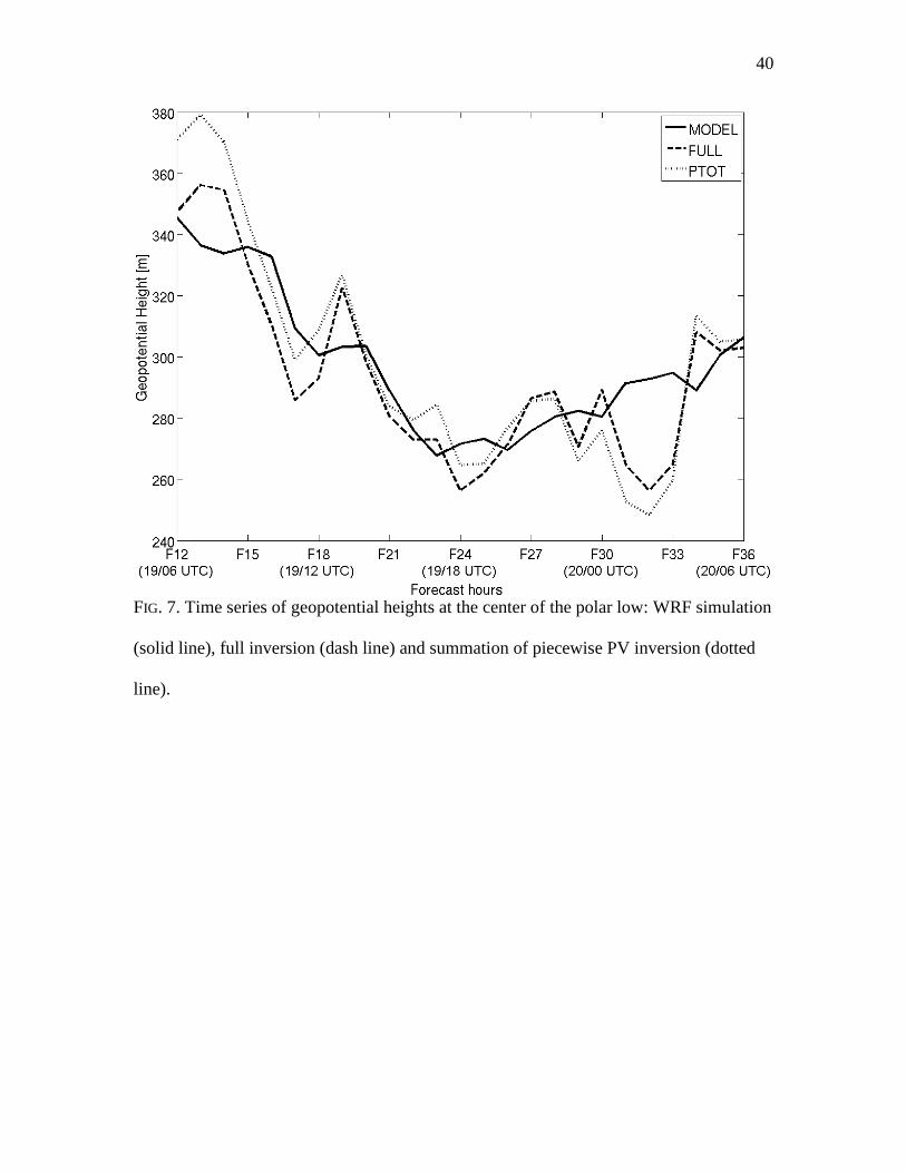
upper-level trough axis where the balance condition is most likely to be violated. Figure 7
is a time series of geopotential heights at the center of the polar low. Note that the full
inversion height agrees well with the model heights at most of the forecast times.
Additionally, the full inversion and the sum of the partitioned PV pieces are generally
within 1 dam of each other, indicating that the piecewise partitioning scheme accounts for
most parts of the total perturbation PV and associated perturbation heights. Given these
similarities, we confidently employ the results of the piecewise PV inversion to diagnose
the development of the polar low.
4.3. Partitioned height changes
Figure 8 shows the 950-hPa height perturbation associated with the Upert PV
anomaly at 12-h intervals from 1800 UTC 18 December to 0600 UTC 20 December. The
Page 16
16
position of the 950-hPa polar low center from the full inversion is indicated by the star
symbol for times at which the polar low center is clearly identified. At 1800 UTC 18
December (Fig. 8a), the center of the Upert PV anomaly was located over the Eurasian
continent with a minimum height perturbation of 119 m at 950 hPa. A negative height
perturbation (of about 40 m) contributed by the Upert PV anomaly was seen over the
northern Sea of Japan, where the polar low later developed. At 0600 UTC 19 December
(Fig. 8b), the minimum height perturbation associated with the Upert PV anomaly was just
moving off the Eurasian continent. A significant deepening of its associated height
perturbation was seen during the 12-h period as the minimum height perturbation
deepened by about 100 m. The polar low center was located to the northeast of the
minimum height perturbation associated with the Upert PV anomaly. In the next 12-h
period (Fig. 8c), the height perturbation continued to deepen. The polar low center was
just north of, and closer to, the minimum height perturbation associated with the Upert PV
anomaly. By 0600 UTC 20 December (Fig. 8d), the height perturbation associated with
the Upert PV anomaly had weakened while moving to the southeast of the polar low
center.
Given that Mpert includes perturbation PV from 950-400 hPa in air with RH 70%,
some synoptic-scale negative perturbation PV, in regions of cold air advection over or
near the ocean, are included in Mpert. Consequently, weak positive height perturbations
associated with the Mpert PV anomaly were seen over the Sea of Japan at 1800 UTC 18
December (Fig. 9a). At the same time, a weak negative height perturbation, collocated
with the cloud shield of an extratropical cyclone, was seen to the east of the Japan.
During the next 12 hours, the positive height anomaly over the Sea of Japan strengthened
Page 17
17
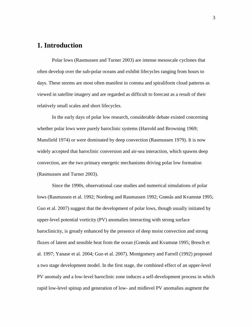
and weak negative height perturbations collocated with the cloud head of developing
cyclone A (shown in Fig. 1a) were evident (Fig. 9b). Although the polar low was
characterized by positive Mpert height perturbations, a narrow trough of low Mpert heights
can be seen extending northward from cyclone A across Hokkaido and into the vicinity of
the polar low.
The center of the Mpert positive height perturbation had weakened by 1800 UTC
19 December as it slid southward across the Sea of Japan (Fig. 9c). Simultaneously, the
negative Mpert height perturbation collocated with the cloud head of cyclone A intensified
substantially while an axis of weak negative Mpert height perturbation extended over the
polar low region. LHR was calculated using the formulation described by Cammas et al.
(1994) employing obtained by solving the balanced equation (following Davis and
Emanuel 1991, Appendix B). Calculated values of LHR (Fig. 10) are well collocated
with the Mpert negative height perturbations at this time, confirming that the negative
height perturbations are primarily attributable to positive PV produced by LHR. In the
next several hours, the negative Mpert height perturbation continued to intensify. As the
polar low moved over land, moderate precipitation occurred near the western coast of
Japan ( Fig. 4b). The negative height perturbation contributed by LHR reached its
minimum of 73 meters over the polar low center at 0200 UTC 20 December (not
shown), after which time the effect of LHR associated with the polar low started to
weaken. By 0600 UTC 20 December (Fig. 9d), negative height anomalies were still
apparent in the vicinity of the polar low while continued intensification of cyclone A was
evident in the even more substantial negative Mpert heights along its developing warm
front at this time.
Page 18
18
For height perturbations associated with the Lpert PV anomaly (Fig. 11), positive
(negative) height perturbations are associated with negative (positive) temperature
anomalies. Throughout the entire analysis period, positive (negative) height perturbations
dominated the western (eastern) part of the domain. Though the positive height
perturbations steadily weakened over time, the negative height perturbations steadily
strengthened. Also, a counterclockwise rotation of the dipole of positive and negative
height perturbations can be seen throughout this time period. At 1800 UTC 18 December
(Fig. 11a), most of the Sea of Japan was dominated by a cold anomaly, though a weak
negative height anomaly is hinted at over Hokkaido. By 0600 UTC 19 December (Fig.
11b), a modest negative height perturbation can be seen in the vicinity of the polar low
with a strong Lpert height gradient to the west and southwest. During the next 12 hours,
although the gradient of the Lpert height perturbations around the polar low continued
increasing, the center of the polar low moved toward positive height perturbations (Fig.
11c). The polar low region was totally covered by positive Lpert height perturbations by
0600 UTC 20 December (Fig. 11d) while the gradient of the height perturbations around
the polar low had also weakened significantly.
Figure 12 shows the 3-hourly evolution of the 950-hPa geopotential height change
at the polar low center during its lifecycle. The tendency and magnitude of the full
inversion height changes agree well with the model data at most times except from 0000
to 0300 UTC 20 December which corresponds to the time of maximum Mpert contribution
to development.
As shown in Fig. 12, the Upert PV anomaly contributed substantially to the 950-
hPa height tendency at the polar low center during the development and dissipation of the
Page 19
19
polar low. From 0900 to 1200 UTC 19 December, the upper-level PV anomaly was the
primary contributor to the development of the polar low. The positive near-surface
temperature anomaly contributed secondarily while a positive height change was
associated with the Mpert PV anomaly. From 1200 to 1800 UTC 19 December, the Upert
PV anomaly and the Mpert PV anomaly contributed nearly equally; counteracting positive
height changes contributed by the Lpert PV anomaly from1200 to 1500 UTC 19
December. From 1800 to 2100 UTC 19 December, there were no significant height
changes contributed by the Upert and Lpert PV anomalies while positive height
perturbations were contributed by the Mpert PV anomaly. In the 6 hours between 2100
UTC 19 December and 0300 UTC 20 December, the Mpert PV anomaly contributed to
deepening the polar low, while the Upert and Lpert PV anomalies contributed modest
weakening. This trend was continued through 0300 to 0600 UTC 20 December during
which time the Upert PV anomaly made the primary contribution to decay of the polar low
while the Mpert PV anomaly contributed secondarily.
4.4. Physical factors influencing the Upert and Mpert PV anomalies
As shown in the preceding section, the Upert PV anomaly contributed most
substantially to both the development and decay of the polar low. The effect of a
tropopause-level PV anomaly on lower-tropospheric heights is dependent on the scale,
magnitude, and shape of the anomaly and is modulated by the intervening stratification
(Hoskins et al. 1985). Figure 13 shows the PV at 350 hPa superimposed upon its
associated 950-hPa Upert height perturbation. The maximum PV values at 350 hPa are
listed in Table 2. In the first 12 hours, the maximum Upert PV decreased slightly from
Page 20
20
6.47 PVU to 6.38 PVU. Then it increased to 6.91 PVU by 1800 UTC 19 December. By
0600 UTC 20 December, the maximum Upert PV had again decreased slightly to 6.74
PVU.
When a PV anomaly is more isotropic (anisotropic), the perturbation heights
associated with it are more intense (weaker) (Morgan and Nielsen-Gammon, 1998;
Martin and Marsili, 2002), a result of the superposition principle. The thinning and
elongation of the Upert PV observed from 1800 UTC 19 December to 0600 UTC 20
December (Fig. 13c and Fig. 13d), is the opposite of superposition and results in an
increased anisotropy to the anomaly. This process was termed “PV attenuation” by
Martin and Marsili (2002) and it contributes to a weakening of the perturbation heights
associated with the Upert PV anomaly.
The largest perturbation geopotential height contributed by the Upert PV anomaly
was, at each time, found at 350 hPa. Thus, the ratio of the 950 to 350-hPa perturbation
height in the column containing the 950-hPa perturbation height minimum can be used to
assess the changes in the penetration depth of the Upert PV anomaly. From Table 2, the
ratio increased steadily from 0.64 at 1800 UTC 18 December to 0.81 at 0600 UTC 20
December. Coincident with these changes, the Square of Brunt-Väisällä frequency
( 2 g dN
dz
) at this column decreased from 3.73x10
-4 s
-2 to 3.34x10
-4 s
-2 at the first 12 h
and increased modestly (3.50x10⁻⁴
s-2
) in the subsequent 12 h. By 0600 UTC 20
December, the N2 increased substantially to 3.77 x10
-4 s
-2.
Thus, the rapid 950-hPa Upert height falls in the first 12 hours of this polar low‟s
development were primarily a result of migration of Upert PV anomaly over the ocean,
where the penetration depth was increased via a reduction in the lower tropospheric static
Page 21
21
stability. At 0600 UTC 20 December, the Upert perturbation height rises at 950 hPa
resulted from the thinning and elongation (i.e. attenuation) of the Upert PV perturbation.
As is the case in extratropical cyclones, LHR modified the environment so as to
encourage development of the polar low in two ways. First, LHR in the column served to
reduce the static stability. In fact, the N2 at the polar low center gradually decreased from
3.66 x 10⁻⁴
s-2
at 0600 UTC 19 December to 3.59 x 10⁻⁴
s-2
at 1800 UTC 19 December,
and further to 3.43 x 10⁻⁴
s-2
at 0600 UTC 20 December. Second, as shown in Fig. 9 and
Fig. 10, the diabatically generated PV anomaly was associated with a negative
geopotential height perturbation in the lower troposphere, which directly, though at most
times secondarily, contributed to the intensification of the surface cyclone.
Based on the preceding analysis, the development processes of the polar low can
be summarized as follows. Prior to the development of the polar low, a positive
tropopause-level PV anomaly over the Eurasian continent, moved southeastward toward
the central Sea of Japan. Near the surface, a weak positive temperature anomaly over the
northern Sea of Japan (near Hokkaido) was generated by warm air advection forced by
the winds associated with the Upert PV anomaly. When the Upert PV anomaly moved over
the Sea of Japan, where the static stability was considerably lower, the negative height
perturbation associated with the Upert PV anomaly intensified substantially which, in turn,
assisted in the intensification of the surface temperature anomaly. The combined effects
of the height perturbation associated with the Upert and Lpert PV anomalies instigated
development of the polar low. This development was characterized by an outbreak of
convection near the low center. The Mpert PV anomaly contributed by LHR initially
enhanced the development of the polar low by superposing an additional negative height
Page 22
22
perturbation in the lower troposphere. The development process of this polar low shares
elements of the two stage development proposed by Montgomery and Farrell (1992),
namely the cyclogenetic influence of the Upert PV anomaly and the contribution to
development made by LHR. However, the analysis presented here also suggests a
departure from this model in two aspects; 1) the Upert PV anomaly contributed
significantly during the developing and decaying stages of the polar low; 2) the
dissipation of the polar low was primarily forced by the weakening of the contribution
from the Upert PV anomaly.
5. Summary and conclusion
The piecewise PV inversion method of Davis and Emanuel (1991) was used in
this study to diagnose the development processes of a polar low over the Sea of Japan. It
was shown that the large scale balanced motions derived from the PV inversion show
good agreement with the fully nonlinear atmospheric flow. The total perturbation PV
field was partitioned into three pieces designed to isolate PV anomalies at the tropopause
(Upert), those associated with mid-tropospheric PV anomalies generated by LHR (Mpert),
and those associated with lower boundary temperature anomalies (Lpert), respectively.
The piecewise PV inversion results clearly demonstrated the effect and relative
importance of these discrete PV anomalies on the development of this polar low.
When the positive PV anomaly near the tropopause moved southeastward toward
the Sea of Japan where the lower troposphere was less stably stratified, the effect of the
upper-level positive PV anomaly on the circulation in the lower troposphere intensified.
A weak positive potential temperature anomaly was generated over the northern Sea of
Page 23
23
Japan as surface cyclogenesis and associated warm air advection began to the east of
Japan. As the Upert PV anomaly moved over the Sea of Japan, the effect of the Upert PV
anomaly on lower tropospheric heights intensified significantly primarily due to a
reduction of the lower tropospheric static stability. Thus, the interaction of the Upert PV
anomaly and the surface warm anomaly induced the development of the polar low over
the Sea of Japan.
During the development of the polar low, LHR associated with cloud and
precipitation processes further reduced the static stability and, via positive perturbation
PV production, superposed an additional negative height perturbation in the lower
troposphere. At the same time, the effect of the Upert PV anomaly made a contribution
toward development equal to that produced by LHR.
When the polar low moved over land, the combined effect of the thinning and
elongation of the Upert PV anomaly decreased the effect of the Upert PV anomaly on the
lower tropospheric geopotential heights. The Mpert PV and Lpert PV anomalies also
contributed to the positive geopotential height changes. As a consequence, the polar low
quickly dissipated.
This study confirms that piecewise PV inversion is a useful tool for examining the
dynamics of polar low formation. With this method, new insights into the effect of
discrete PV anomalies on the development of polar lows can be obtained. More polar low
cases, with different synoptic environments, are currently being investigated with the
piecewise PV inversion method. It is hoped that the results of these analyses will add
important detail to the conceptual and physical model of the development of polar lows.
Page 24
24
Acknowledgement
The authors thank Dr. Wataru Yanase for sharing the polar low case. Thanks also to Mr.
Pete Pokrandt, Mr. Yunfei Zhang, Mr. Dierk Polzin and the WRF support staff for their
assistance with setting up the WRF simulations. The authors also thank Dr. Derek Posselt
and Mr. Jason Otkin for assistance with the PV inversion programs. The comments from
two anonymous reviewers are appreciated. The GOES-9 imagery was obtained from
http://weather.is.kochi-u.ac.jp/sat/gms.fareast/. The precipitation data from AMeDAS
radar product was obtained from JAXA/EORC. This study was supported by NASA
grant NNX08AD36G.
Page 25
25
References
Bracegirdle, T. J., and S. L. Gray, 2009: The dynamics of a polar low assessed using
potential vorticity inversion. Quart. J. Roy. Meteorol. Soc., 135, 880-893.
Bresch, J. F., R. J. Reed, and M. D. Albright, 1997: A Polar-Low Development over the
Bering Sea: Analysis, Numerical Simulation, and Sensitivity Experiments. Mon.
Wea. Rev., 125, 3109–3130.
Bretherton, F. P., 1966: Baroclinic instability and the shortwave cutoff in terms of
potential vorticity. Quart. J. Roy. Meteor. Soc., 92, 335–345.
Cammas, J.-P., D. Keyser, G. Lackmann, and J. Molinari, 1994: Diabatic redistribution
of potential vorticity accompanying the development of an outflow jet within a
strong extratropical cyclones. Proc. Int. Symp. on Life Cycles of Extratropical
Cyclones, Vol. II, Bergen, Norway, Aase Grafiske A/S, 403-409.
Charney, J., 1955: The use of the primitive and balance equations. Tellus, 7, 22–26.
Davis, C. A. and K. A. Emanuel, 1991: Potential vorticity diagnostics of cyclogenesis.
Mon. Wea. Rev., 119, 1929–1953.
Davis, C. A., M. T. Stoelinga, and Y.-H. Kuo, 1993: The integrated effect of
condensation in numerical simulations of extratropical cyclogenesis. Mon. Wea.
Rev., 121, 2309–2330.
Page 26
26
Deng, A., N. L. Seaman, G. K. Hunter and D. R. Stauffer, 2004: Evaluation of
Interregional Transport Using the MM5–SCIPUFF System. J. Appl. Meteor., 43,
1864–1886. doi: 10.1175/JAM2178.1
Dudhia, J., 1989: Numerical study of convection observed during the winter monsoon
experiment using a mesoscale two-dimensional model. J. Atmos. Sci., 46, 3077–
3107.
Dudhia, J., S.-Y. Hong, and K.-S. Lim, 2008: A new method for representing mixed-
phase particle fall speeds in bulk microphysics parameterizations. J. Meteor. Soc.
Japan, 86A, 33-44.
Ertel, H., 1942: Ein Neuer hydrodynamischer Wirbelsatz. Meteor. Z., 59, 271–281.
Grønås, S., and N. G. Kvamstø, 1995: Numerical simulations of the synoptic conditions
and development of Arctic outbreak polar lows. Tellus, 47A, 797–814.
Guo, J. T., G. Fu, Z. L. Li, L. M. Shao, Y. H. Duan and J. G. Wang, 2007: Analyses and
numerical modeling of a polar low over the Japan Sea on 19 December 2003.
Atmos. Res., 85(3-4), 395-412.
Harrold, T. W., and K. A. Browning, 1969: The polar low as a baroclinic disturbance.
Quart. J. Roy. Meteor. Soc, 95, 710–723.
Hong, S.-Y., and J.-O. J. Lim, 2006: The WRF Single-Moment 6-Class Microphysics
Scheme (WSM6), J. Korean Meteor. Soc., 42, 129–151.
Hong, S.-Y., Y. Noh, and J. Dudhia, 2006: A new vertical diffusion package with an
explicit treatment of entrainment processes. Mon. Wea. Rev., 134, 2318–2341.
Page 27
27
Hoskins B. J, M. E McIntyre, and A. W Robertson, 1985: On the use and significance of
isentropic potential vorticity maps. Quart. J. Roy. Meteor. Soc., 111, 877–946.
Kain, J. S., and J. M. Fritsch, 1990: A one-dimensional entraining/detraining plume
model and its application in convective parameterization. J. Atmos. Sci., 47,
2784–2802.
Kain, J. S., and J. M. Fritsch, 1993: Convective parameterization for mesoscale models:
The Kain–Fritsch scheme. The Representation of Cumulus Convection in
Numerical Models, Meteor. Monogr., No. 46, Amer. Meteor. Soc., 165–170.
Korner, S. O., and J. E. Martin, 2000: Piecewise frontogenesis from a potential vorticity
perspective: Methodology and a case study. Mon. Wea. Rev., 128, 1266–1288.
Mansfield, D. A., 1974: Polar lows: The development of baroclinic disturbances in cold
air outbreaks. Quart. J. Roy. Meteor. Soc., 100, 541–554.
Martin, J. E., and N. Marsili, 2002: Surface cyclolysis in the North Pacific Ocean. Part II:
Piecewise potential vorticity diagnosis of a rapid cyclolysis event. Mon. Wea.
Rev., 130, 1264–1281.
Martin, J. E., and J. A. Otkin, 2004: The Rapid Growth and Decay of an Extratropical
Cyclone over the Central Pacific Ocean. Wea. Forecasting, 19, 358–376.
Mlawer, E. J., S. J. Taubman, P. D. Brown, M. J. Iacono, and S. A. Clough, 1997:
Radiative transfer for inhomogeneous atmosphere: RRTM, a validated correlated-
k model for the longwave. J. Geophys. Res., 102 (D14), 16663–16682.
Page 28
28
Montgomery, M. T., and B. F. Farrell, 1992: Polar low dynamics. J. Atmos. Sci., 49,
2484–2505.
Morgan, M. C., and J. Nielsen-Gammon, 1998: Using tropopause maps to diagnose
midlatitude weather systems. Mon. Wea. Rev., 126, 2555–2579.
Nordeng, T. E., and E. A. Rasmussen, 1992: A most beautiful polar low. A case study of
a polar low development in the Bear Island region. Tellus, 44A, 81–99.
Posselt, D. J., and J. E. Martin, 2004: The effect of latent heat release on the evolution of
a warm occluded thermal structure. Mon. Wea. Rev., 132, 578–599.
Rasmussen, E. A., 1979: Polar low as an extratropical CISK disturbance. Quart. J. Roy.
Meteor. Soc., 105, 531–549.
Rasmussen, E. A., T. S. Pedersen, L. F. Pedersen, and J. Turner, 1992: Polar lows and
arctic instability lows in the Bear Island region. Tellus, 44A, 133–154.
Rasmussen, E. A., and J. Turner, 2003: Polar lows: Mesoscale Weather Systems in the
Polar Regions. Cambridge University Press, 612 pp.
Rossby, C. G., 1940: Planetary flow patterns in the atmosphere. Quart. J. Roy. Meteor.
Soc., 66, 68–87.
Skamarock, W. C., J. B. Klemp, J. Dudhia, D. O. Gill, D. M. Barker, M. G. Duda, X. Y.
Huang, W. Wang, and J. G. Powers, 2008: A description of the advanced research
WRF version 3. NCAR/TN-468+STR, 126 pp.
Page 29
29
Stoelinga, M. T., 1996: A potential vorticity-based study of the role of diabatic heating
and friction in a numerically simulated baroclinic cyclone. Mon. Wea. Rev., 124,
849–874.
Sutcliffe, R., 1947: A contribution to the problem of development. Quart. J. Roy. Meteor.
Soc., 73, 370–383.
Trenberth, K. E., 1978: On the interpretation of the diagnostic quasi-geostrophic omega
equation. Mon. Wea. Rev., 106, 131–137.
Wu, L. T., and G. W. Petty, 2010: Intercomparison of Bulk Microphysics Schemes in
Model Simulations of Polar Lows. Mon. Wea. Rev., 138, 2211-2228.
Yanase, W., G. Fu, H. Niino, and T. Kato, 2004: A Polar Low over the Japan Sea on 21
January 1997. Part II: A Numerical Study. Mon. Wea. Rev., 132, 1552–1574.
Page 30
30
FIGURE CAPTIONS
FIG. 1. NCEP FNL analyses data at 0600 UTC 19 December 2003. (a) SLP (solid lines,
contoured at 4 hPa intervals) and 1000-500-hPa thickness (dashed lines, unit: 10 m,
contoured at 60 m intervals); Symbol „A‟ and „P‟ represent the center of extratropical
cyclone A and polar low P, respectively. (b) The 500-hPa geopotential height (solid lines,
contoured at 60 m intervals), temperature (dashed lines, contoured at 4 K intervals) and
absolute vorticity (shaded); Symbol „N‟ and „S‟ represent the positions of the two
vorticity maxima, respectively. (c) The 350-hPa PV; PV is labeled in PVU (1 PVU = 10-6
m2
K kg-1
s-1
) and contoured by every 1 PVU beginning at 1 PVU.
FIG. 2. NCEP FNL analyses data at 1800 UTC 19 December 2003. (a) As for Fig. 1a. (b)
As for Fig. 1b. (c) As for Fig. 1c.
FIG. 3. NCEP FNL analyses data at 0000 UTC 20 December 2003. (a) As for Fig. 1a. (b)
As for Fig. 1b. (c) As for Fig. 1c.
FIG. 4. (a) GOES-9 IR imagery at 0000 UTC 20 December 2003 shows a spiraliform
polar low over Japan, with clear eye in the center. (b) The precipitation rate from the
Automatic Meteorological Data Acquisition System (AMeDAS) radar product at 0350
UTC 20 Dec 2003.
Page 31
31
FIG. 5. Inner (d02) and outer (d01) domains of the WRF simulation used in this analysis.
The centers of cyclone A and the polar low P at the sea level are also shown in the
domain. Cyclone A in gray; polar low P in black; simulated data shown with star symbol;
FNL analyzed data shown with dot symbol. All the positions are identified at 6-h
intervals according to the FNL analyses and the 25-km WRF simulations. Cyclone A is
identified from 1800 UTC 18 December to 1200 UTC 20 December while the polar low
P is from 0600 UTC 19 December to 0600 UTC 20 December. The time series of the
same dataset are connected by solid lines. At each time, the centers of the FNL analysis
and WRF simulation are connected by dotted lines.
FIG. 6. (a) The WRF 950-hPa geopotential height contoured every 40 m. (b) The full
inverted geopotential height contoured every 40 m. (c) The difference between the full
inverted field and WRF field contoured every 20 m. All the fields are valid at 0000 UTC
20 December 2003.
FIG. 7. Time series of geopotential heights at the center of the polar low: WRF simulation
(solid line), full inversion (dash line) and summation of piecewise PV inversion (dotted
line).
FIG. 8. The 950-hPa geopotential height perturbation associated with the Upert PV
anomaly. Negative (positive) geopotential height perturbations are indicated by dashed
(solid) lines contoured every 40 m. The star indicates the location of the polar low center
Page 32
32
at each time. Valid at (a) 1800 UTC 18 December; (b) 0600 UTC 19 December; (c) 1800
UTC 19 December; (d) 0600 UTC 20 December.
FIG. 9. The 950-hPa geopotential height perturbation associated with the Mpert PV
anomaly. Negative (positive) geopotential height perturbations are indicated by dashed
(solid) lines contoured every 10 m. The star indicates the location of the polar low center
at each time. Valid at (a) 1800 UTC 18 December; (b) 0600 UTC 19 December; (c) 1800
UTC 19 December; (d) 0600 UTC 20 December.
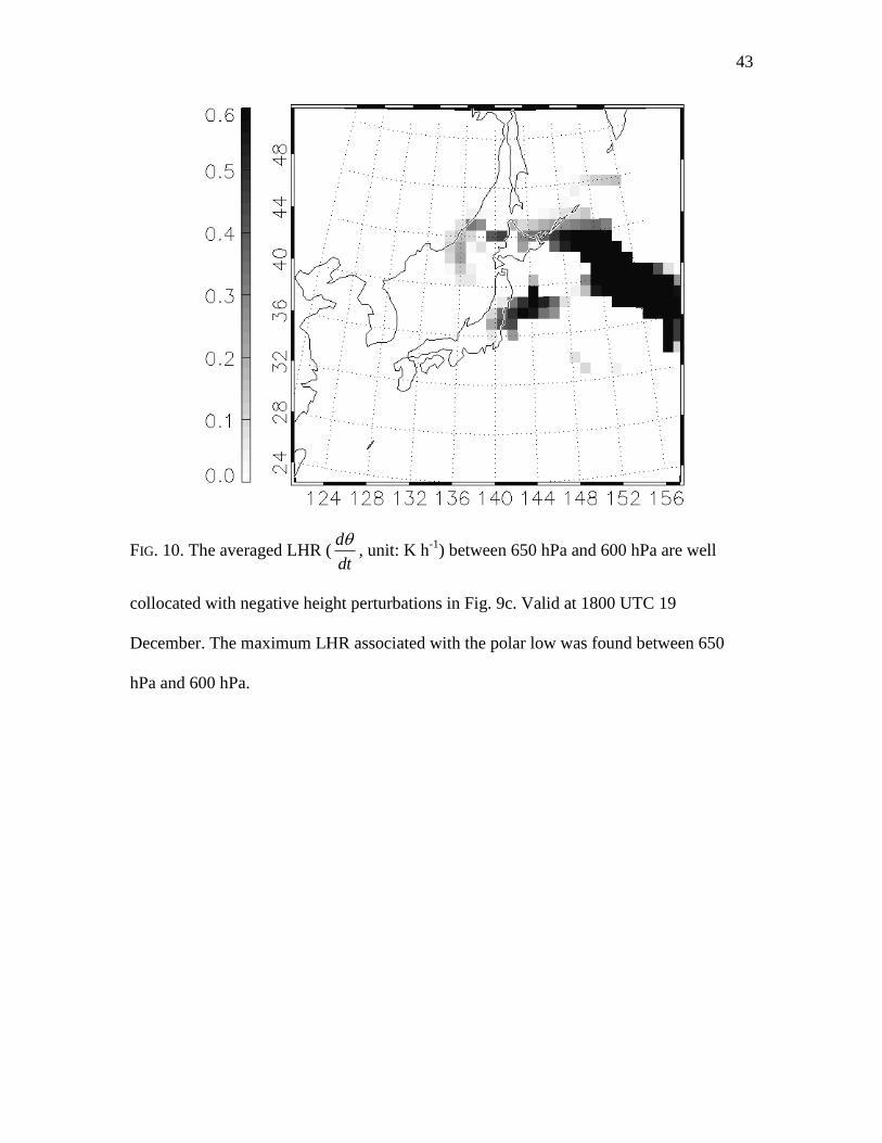
FIG. 10. The averaged LHR (d
dt
, unit: K h
-1) between 650 hPa and 600 hPa are well
collocated with negative height perturbations in Fig. 9c. Valid at 1800 UTC 19
December. The maximum LHR associated with the polar low was found between 650
hPa and 600 hPa.
FIG. 11. The 950-hPa geopotential height perturbation associated with the Lpert PV
anomaly. Negative (positive) geopotential height perturbations are indicated by dashed
(solid) lines contoured every 10 m. The star indicates the location of the polar low center
at each time. Valid at (a) 1800 UTC 18 December; (b) 0600 UTC 19 December; (c) 1800
UTC 19 December; (d) 0600 UTC 20 December.
FIG. 12. The 3-hourly height changes at the 950-hPa center of polar low: WRF outputs in
grey thin dashed line; full inversions in grey thin solid line; perturbation heights
Page 33
33
associated with the Upert in black thick solid line; Mpert in black thick dashed line; Lpert in
black thick dotted line.
FIG. 13. As for Fig. 8 but with 350 hPa perturbation PV superimposed. Valid at (a) 1800
UTC 18 December; (b) 0600 UTC 19 December; (c) 1800 UTC 19 December; (d) 0600
UTC 20 December.
List of Figures
Page 34
34
FIG. 1. NCEP FNL analyses data at
0600 UTC 19 December 2003. (a)
SLP (solid lines, contoured at 4 hPa
intervals) and 1000-500-hPa
thickness (dashed lines, unit: 10 m,
contoured at 60 m intervals); Symbol
„A‟ and „P‟ represent the center of
extratropical cyclone A and polar
low P, respectively. (b) The 500-hPa
geopotential height (solid lines,
contoured at 60 m intervals),
temperature (dashed lines, contoured
at 4 K intervals) and absolute
vorticity (shaded); Symbol „N‟ and
„S‟ represent the positions of the two
vorticity maxima, respectively. (c)
The 350-hPa PV; PV is labeled in
PVU (1 PVU = 10-6
m2
K kg-1
s-1
)
and contoured by every 1 PVU
beginning at 1 PVU.
Page 35
35
FIG. 2. NCEP FNL analyses data at
1800 UTC 19 December 2003. (a)
As for Fig. 1a. (b) As for Fig. 1b. (c)
As for Fig. 1c.
Page 36
36
FIG. 3. NCEP FNL analyses data at
0000 UTC 20 December 2003. (a) As
for Fig. 1a. (b) As for Fig. 1b. (c) As
for Fig. 1c
Page 37
37
FIG. 4. (a) GOES-9 IR imagery at 0000 UTC 20 December 2003 shows a spiraliform
polar low over Japan, with clear eye in the center. (b) The precipitation rate from the
Automatic Meteorological Data Acquisition System (AMeDAS) radar product at 0350
UTC 20 Dec 2003.
Page 38
38
FIG. 5. Inner (d02) and outer (d01) domains of the WRF simulation used in this analysis.
The centers of cyclone A and the polar low P at the sea level are also shown in the
domain. Cyclone A in gray; polar low P in black; simulated data shown with star symbol;
FNL analyzed data shown with dot symbol. All the positions are identified at 6-h
intervals according to the FNL analyses and the 25-km WRF simulations. Cyclone A is
identified from 1800 UTC 18 December to 1200 UTC 20 December while the polar low
P is from 0600 UTC 19 December to 0600 UTC 20 December. The time series of the
same dataset are connected by solid lines. At each time, the centers of the FNL analysis
and WRF simulation are connected by dotted lines.
Page 39
39
FIG. 6. (a) The WRF 950-hPa geopotential height contoured every 40 m. (b) The full
inverted geopotential height contoured every 40 m. (c) The difference between the full
inverted field and WRF field contoured every 20 m. All the fields are valid at 0000 UTC
20 December 2003.
Page 40
40
FIG. 7. Time series of geopotential heights at the center of the polar low: WRF simulation
(solid line), full inversion (dash line) and summation of piecewise PV inversion (dotted
line).
Page 41
41
FIG. 8. The 950-hPa geopotential height perturbation associated with the Upert PV
anomaly. Negative (positive) geopotential height perturbations are indicated by dashed
(solid) lines contoured every 40 m. The star indicates the location of the polar low center
at each time. Valid at (a) 1800 UTC 18 December; (b) 0600 UTC 19 December; (c) 1800
UTC 19 December; (d) 0600 UTC 20 December.
Page 42
42
FIG. 9. The 950-hPa geopotential height perturbation associated with the Mpert PV
anomaly. Negative (positive) geopotential height perturbations are indicated by dashed
(solid) lines contoured every 10 m. The star indicates the location of the polar low center
at each time. Valid at (a) 1800 UTC 18 December; (b) 0600 UTC 19 December; (c) 1800
UTC 19 December; (d) 0600 UTC 20 December.
Page 43
43
FIG. 10. The averaged LHR (d
dt
, unit: K h
-1) between 650 hPa and 600 hPa are well
collocated with negative height perturbations in Fig. 9c. Valid at 1800 UTC 19
December. The maximum LHR associated with the polar low was found between 650
hPa and 600 hPa.
Page 44
44
FIG. 11. The 950-hPa geopotential height perturbation associated with the Lpert PV
anomaly. Negative (positive) geopotential height perturbations are indicated by dashed
(solid) lines contoured every 10 m. The star indicates the location of the polar low center
at each time. Valid at (a) 1800 UTC 18 December; (b) 0600 UTC 19 December; (c) 1800
UTC 19 December; (d) 0600 UTC 20 December.
Page 45
45
FIG. 12. The 3-hourly height changes at the 950-hPa center of polar low: WRF outputs in
grey thin dashed line; full inversions in grey thin solid line; perturbation heights
associated with the Upert in black thick solid line; Mpert in black thick dashed line; Lpert in
black thick dotted line.
Page 46
46
FIG. 13. As for Fig. 8 but with 350 hPa perturbation PV superimposed. Valid at (a) 1800
UTC 18 December; (b) 0600 UTC 19 December; (c) 1800 UTC 19 December; (d) 0600
UTC 20 December.
Page 47
47
List of tables
TABLE 1. The FNL analyzed and WRF simulated SLPs in the center of cyclone A and
the polar low P at each time.
Time
SLP (hPa) in the center of
cyclone A
SLP (hPa) in the center of the
polar low
FNL WRF FNL WRF
1800 UTC 18 Dec. 1001 999
0000 UTC 19 Dec. 999 998
0600 UTC 19 Dec. 992 994 995 992
1200 UTC 19 Dec. 989 988 994 985
1800 UTC 19 Dec. 981 978 993 983
0000 UTC 20 Dec. 975 969 993 984
0600 UTC 20 Dec. 972 962 996 984
1200 UTC 20 Dec. 973 962
Page 48
48
TABLE 2. The maximum EPV at 350 hPa; the 950-hPa and 350-hPa perturbation height
associated with Upert, their ratio and the corresponded Square of bulk Brunt-Väisällä
frequency (N2) at each time. The N
2 is averaged from bottom to eta level 17 (eta
value=0.30, which is about 350 hPa) at the 950-hPa perturbation height minimum
column.
Time Max EPV at
350 hPa (PVU)
950 hPa
[m]
350 hPa
[m]
Ratio N2 [10
-4 s
-2]
1800 UTC 18 Dec. 6.47 119 185 0.64 3.73
0600 UTC 19 Dec. 6.38 218 315 0.69 3.34
1800 UTC 19 Dec. 6.91 265 355 0.75 3.50
0600 UTC 20 Dec. 6.74 208 254 0.81 3.77