Pinned Fronts in Heterogeneous Media of Jump Type Peter van Heijster * , Arjen Doelman † , Tasso J. Kaper ‡ , Yasumasa Nishiura § , Kei-Ichi Ueda ¶ * Division of Applied Mathematics, Brown University, 182 George Street, Providence, RI 02912, USA † Mathematisch Instituut, Universiteit Leiden, P.O. Box 9512, 2300 RA Leiden, Netherlands ‡ Department of Mathematics & Center for BioDynamics, Boston University, 111 Cummington Street, Boston, MA 02215, U.S.A. § Laboratory of Nonlinear Studies and Computation Research Institute for Electronic Science, Hokkaido University, Sapporo 060-0812, Japan ¶ Research Institute for Mathematical Sciences, Kyoto University, Kyoto 606-8502, Japan October 26, 2010 Abstract In this paper, we analyze the impact of a (small) heterogeneity of jump type on the most simple localized solutions of a three-component FitzHugh-Nagumo-type system. We show that the heterogeneity can pin a 1-front solution, which travels with constant (non-zero) speed in the homogeneous setting, to a fixed, explicitly determined, distance from the heterogeneity. Moreover, we establish the stability of this heterogeneous pinned 1-front solution. In addition, we analyze the pinning of 1-pulse, or 2-front, solutions. The paper is concluded with simulations in which we consider the dynamics and interactions of N -front patterns in domains with M heterogeneities of jump type (N =3, 4, M ≥ 1). key words. three-component reaction-diffusion systems, pinned fronts, heterogeneous media, geometric singular perturbation theory, semi-strong front interactions AMS subject classification. 35K57, 35K45, 35B36, 35B25, 35Q92 1
Transcript
Pinned Fronts in Heterogeneous Media of Jump Type
Peter van Heijster∗, Arjen Doelman†, Tasso J. Kaper‡,Yasumasa Nishiura§, Kei-Ichi Ueda¶
∗Division of Applied Mathematics, Brown University,182 George Street, Providence, RI 02912, USA
†Mathematisch Instituut, Universiteit Leiden,P.O. Box 9512, 2300 RA Leiden, Netherlands
‡Department of Mathematics & Center for BioDynamics,Boston University, 111 Cummington Street,
Boston, MA 02215, U.S.A.
§Laboratory of Nonlinear Studies and Computation Research Institutefor Electronic Science, Hokkaido University, Sapporo 060-0812,
Japan
¶Research Institute for Mathematical Sciences, Kyoto University,Kyoto 606-8502, Japan
October 26, 2010
Abstract
In this paper, we analyze the impact of a (small) heterogeneity of jump type on the mostsimple localized solutions of a three-component FitzHugh-Nagumo-type system. We show thatthe heterogeneity can pin a 1-front solution, which travels with constant (non-zero) speed inthe homogeneous setting, to a fixed, explicitly determined, distance from the heterogeneity.Moreover, we establish the stability of this heterogeneous pinned 1-front solution. In addition,we analyze the pinning of 1-pulse, or 2-front, solutions. The paper is concluded with simulationsin which we consider the dynamics and interactions of N -front patterns in domains with Mheterogeneities of jump type (N = 3, 4, M ≥ 1).
In many (classical) mathematical models, especially those of reaction-diffusion type, the medium inwhich the process under consideration takes place is (implicitly) assumed to be homogeneous. Thisis of course a simplification; natural media, even in their equilibrium states or background states,generally contain heterogeneities. For instance in the field of superconductivity, there is quite an ex-tensive literature, dating back to the seventies, on the impact of spatially localized heterogeneities,or ‘impurities’, on the dynamics of localized structures (the so-called fluxons), see [14]. There is alsoa special interest in the influence of spatial heterogeneities on the dynamics of localized structuressuch as fronts and pulses in reaction-diffusion equations, see [1, 2, 16, 18, 24, 25] and the referencestherein. The pinning phenomenon, in which a traveling solution gets trapped by the heterogeneitywhile its homogeneous equivalent would have kept on traveling, can be considered as one of its mostdramatic effects.
While pinning has been studied analytically in the special case of scalar equations (see [2, 24] andthe references therein), it has been studied much less extensively for systems of reaction-diffusionequations [9, 10, 11], see Remark 1.1. Numerically, pinning for systems of reaction-diffusion equa-tions has been studied more thoroughly. A model for which extensive numerical simulations areavailable is a generalized FitzHugh-Nagumo-type (FHN) system. This model has been proposedto describe, on a phenomenological level, the behavior of gas-discharge systems, see [19, 20] andreferences therein. In two space dimensions this system is given by
Ut = DU∆U + f(U)− κ3V − κ4W + κ1(x, y) ,τVt = DV ∆V + U − V ,θWt = DW∆W + U −W ,
(1.1)
where f(U) is typically a cubic nonlinearity and κ1(x, y) models the heterogeneity. System (1.1)is also a natural extension of the FHN equations to systems with two inhibitors. Since (1.1) is asystem, the pinning phenomenon cannot be studied by the methods employed in [2], which relyheavily on the scalar nature of the equations under consideration. For instance, scalar systemshave a gradient structure, and their solutions can be controlled by sub- and super-solutions. Theseproperties are crucial ingredients in the analysis of [2]. Moreover, unlike the models used for pin-ning in superconductivity, (1.1) is not close to a completely integrable partial differential equation(PDE), so that the impact of (localized, spatial) heterogeneities cannot be studied by a perturbationmethod based on this fact [14]. In this paper, we employ a dynamical systems approach to analyzethe impact of localized heterogeneities on localized solutions of (1.1). Note that this approach issimilar to that of [1] which considers a model for Josephson junctions with jump type heterogeneities.
In [25], the influence of a small smoothened jump type heterogeneity on traveling pulses of (1.1)in one space dimension is studied. It is observed that a traveling pulse colliding with the hetero-geneity can penetrate, be annihilated, rebound, oscillate or get pinned. More precisely, the pinnedsolutions are observed when the heterogeneity jumps down, and the pinned solutions are ‘in front’of the heterogeneity, that is, they are located immediately to the left of the heterogeneity. In[18], the influences of two different heterogeneities on traveling pulses are investigated for the samemodel, that is, the influences of a symmetric bump type, or 2-jump, heterogeneity and a periodicheterogeneity are studied. For the bump heterogeneity, also penetration, rebound, annihilation,oscillation and pinning are observed. However, there are now two types of pinned solutions. One is
2
0
0.5
1
1.5
2
2.5
3 x 10
4
-1000
-500
0
500
1000
-1
0
1
0
0.5
1
1.5
2
2.5
3 x 10
4
-1000
-500
0
500
1000
-1
0
1
0
0.5
1
1.5
2
2.5
3 x 10
4
-1000
-500
0
500
1000
-1
0
1
Figure 1: A traveling front solution of (1.2) that asymptotes to a stationary front, located at theheterogeneity, and hence is said to be pinned there. The system parameters are chosen as follows(α, β, γ1, γ2, τ, θ,D, ε) = (3, 1, 1,−3, 1, 1, 5, 0.01). The thick black dashed line indicates the locationof the heterogeneity.
a pinned solution ‘in front’ of a bump, and one is a pinned solution in the bump region. The pinnedsolution which is observed depends on the bump being up or down. For the periodic heterogeneity,also spatio-temporal chaos is observed.
In this paper, we present an analytic understanding of the pinning phenomenon in heterogeneousmedia. That is, we develop a method by which it is possible to predict for which parameter valuespinning can be expected. We will focus on the most elementary (localized) solutions, that is, the1-front solutions and 2-front (or 1-pulse) solutions, and we will also use these insights to study moreextended patterns. Motivated by the numerical simulations discussed in the previous paragraph, weanalyze the pinning phenomenon in the three-component FHN-system (1.1) in a particular scaling
with γ1,2 ∈ R\{0}, see Remark 1.2. Here, all parameters are assumed to be O(1) with respect toε. This typical scaling of (1.1) has been introduced in [5]. See Figure 1 for a pinned 1-front solution.
We choose this particular heterogeneous model since it is sufficiently transparent for the purposesof performing explicit mathematical analysis, while at the same time it is sufficiently complex tosupport complex localized structures. More specifically, our results (and analysis) simplify in thespecial cases when either α = 0 or β = 0. These correspond to reductions of the 3-component modelto a simpler 2-component model. In particular, our results (Theorem 1.4 and 1.5) show that also
3
the 2-component model exhibits pinned front and 2-front solutions. However, as will be clear lateron, the dynamics of the 2-front solutions (and more general N -front solutions) are much richer inthe 3-component model, see also [5, 21]. Moreover, to analyze scattering and other more complexphenomena observed in [17], the analysis developed here for the full 3-component model will berequired. Also, as is clear from the above discussion, this model has been extensively studied vianumerical simulations. The specific choice of the heterogeneity comes, on the one hand, from thejump type heterogeneity considered in [25]. On the other hand, it is motivated by our intention tokeep the analysis manageable. Furthermore, a (smoothened) step function can be seen as a basicingredient for more general heterogeneities such as periodic and random media [25]. By the choiceswe made, we are able for example to explicitly determine the pinning distance of the localizedstructures to the heterogeneity and how that depends on the system parameters.
In [5, 21, 22], a detailed analysis of the existence [5], stability [21] and interaction [22] of local-ized structures for the homogeneous problem ((1.2) with γ(ξ) ≡ γ, constant) is given. Of the mainresults of these papers, three are needed for this paper:
Theorem 1.1 [22] For ε > 0 small enough, the homogeneous model ((1.2) with γ(ξ) ≡ γ, con-stant) possesses a stable traveling 1-front solution which travels with speed 3
2
√2εγ; it possesses no
stationary 1-front solutions.
Theorem 1.2 [22] For ε > 0 small enough, the width ∆Γ of a 2-front solution to the homogeneousmodel evolves according to
∆Γ(t) = 3√
2ε(αe−ε∆Γ + βe−εD∆Γ − γ) , (1.4)
where ∆Γ := Γ2 − Γ1, with Γi the i-th intersection of the Ucomponent with zero.
Theorem 1.3 [5, 21] For ε > 0 small enough, the homogeneous model possesses a 1-parameterfamily of stationary 2-front, or 1-pulse, solutions with width ξγhom > 0, if there is a ξγhom solving
αe−εξγhom + βe−
εD ξ
γhom = γ . (1.5)
This solution is stable if
αe−εξγhom +
β
De−
εD ξ
γhom > 0.
Note that the stationary solutions (1.5) with ∆Γ = ξγhom are the fixed points of (1.4).
There are several important differences between the heterogeneous system (1.2) and its homo-geneous equivalent (γ(ξ) ≡ γ). First, due to the discontinuity in γ(ξ) at ξ = 0, we cannot expectthe solutions to the PDE to be smooth. More precisely, due to the heterogeneity the solutions canonly be C0 in time and C1 in space. Since we are interested in stationary solutions, we can rewrite(1.2) into a six dimensional system of ODEs, see for example (2.2). The solutions to these resultingsystems will only be C0 (in space).
The second, and most important, difference is that the heterogeneous model is no longer trans-lation invariant. This loss of translation invariance challenges the methods developed in [5, 21] inwhich the existence and stability of localized homogeneous structures was studied. By this loss, the
4
spatial derivative of the localized stationary structure is no longer an eigenfunction of the linearizedstability problem with corresponding eigenvalue zero, since this derivative is only C0 and not C1.This has two consequences for the stability analysis. First, we have to determine in which fashionthis zero eigenvalue perturbs, since it will yield an instability if it moves into the right half plane.Second, in [21] the translation invariance was used to derive an extra solvability condition from theexistence analysis that was used as a crucial ingredient in the stability analysis. Therefore, we haveto find a new way to determine the heterogeneous equivalent of this solvability condition.
A third difference is that, for the heterogeneous system it is a priori not clear what the ‘triv-ial’ background solutions are, see also Remark 1.2. However, their asymptotic behavior can bedetermined. As ξ → ±∞, the background solutions limit on
see also [5]. Note that u±,0γi are precisely the solutions to the cubic polynomial
u− u3 − ε(αu+ βw + γi), i = 1, 2.
Since the O(ε) solution (1.7) is unstable it will not be considered in this paper.
System (1.2) has two important symmetries
(U, V,W, γ1, γ2)→ (−U,−V,−W,−γ1,−γ2) (1.8)
and
(ξ, γ1, γ2)→ (−ξ, γ2, γ1) . (1.9)
The first symmetry allows us to restrict to solutions which asymptote to u−γ1(1, 1, 1) as ξ → −∞.For example, we construct stable pinned 1-front solutions which asymptote to u−γ1(1, 1, 1). By thefirst symmetry, we then immediately obtain a stability condition for pinned 1-front solutions whichasymptote to u+
−γ1(1, 1, 1) as ξ → −∞. The second symmetry allows us to obtain additional resultsfor the mirrored solution by interchanging the role of γ1 and γ2. For example, from the existencecondition for a 2-front solution with its front pinned at the heterogeneity, we obtain the existencecondition for a 2-front solution with its back pinned at the heterogeneity by interchanging γ1 andγ2. Therefore, without loss of generality we can restrict the numerical simulations to γ1 > γ2 as wedid in Section 4.1.
This paper is organized as follows. In the next two sections, we establish the conditions underwhich the heterogeneity pins a traveling 1-front solution, and explicitly determine its distance fromthe heterogeneity. We recall from Theorem 1.1 that stationary 1-front solutions do not exist for thehomogeneous problem (γ 6= 0, see Remark 1.2). The main pinning result is,
Theorem 1.4 For ε > 0 small enough, there exists a stable pinned 1-front solution which asymp-totes to (U, V,W ) = u−γ1(1, 1, 1) as ξ → −∞ and whose front is pinned near the heterogeneity if andonly if γ2 < 0 < γ1.
5
Figure 2: Heuristically, we expect pinning of a 1-front solution if γ1 > 0 > γ2. That is, we expectpinning in frame II. Note that only (the singular limit of) the U component of the front is depicted.
See Theorems 2.1 and 3.1 for a more detailed formulation of this result. Intuitively, this theoremcan be explained from the results on traveling 1-front solutions in the homogeneous system, seeTheorem 1.1. These 1-front solutions (which asymptote to (U, V,W ) = u−γ1(1, 1, 1) as ξ → −∞)travel in the direction of the sign of γ. So, fronts travel to the right if γ is positive and to the leftif γ is negative. Therefore, we expect pinning for the heterogeneous model at the heterogeneity if,and only if, γ1 is positive and γ2 is negative. Under these conditions, a 1-front solution away fromthe heterogeneity always moves toward it. All the other configurations of γ1 and γ2 yield movementof the front toward infinity. See also Figure 2.
In Section 4, we determine the existence condition for stationary 2-front solutions whose frontis pinned near the heterogeneity, where we recall that a 2-front solution consists of a front (positivederivatives) concatenated to the right with a back (negative derivatives). Again, we are able toexplicitly compute pinning distance. The main result is,
Theorem 1.5 For ε > 0 small enough and γ1 > γ2, there exists a pinned 2-front solution whichasymptotes to (U, V,W ) = u−γ1(1, 1, 1) as ξ → −∞ and whose front is located near the heterogeneityif and only if there exists a ξ2f > 0 solving
αe−εξ2f + βe−εD ξ2f = γ2 . (1.10)
Moreover, the width of the 2-front solution is ξ2f .
See Theorem 4.1 for a more detailed formulation of this result. Note that condition (1.10) coincideswith the existence condition of a stationary 2-front solution in the homogeneous case with γ = γ2,see Theorem 1.3. Also observe the different role of the heterogeneity between the pinning of the1-front solution and the pinning of the 2-front solution. The heterogeneity ‘creates’ a new station-ary 1-front solution, while it ‘selects’ a particular stationary 2-front solution from a 1-parameterfamily, see Theorems 1.1 and 1.3. Moreover, Theorem 1.5 confirms the numerical observations ofpinned pulses in front of a heterogeneity which jumps down [25] (note the sign difference in frontof κ1(x, y) and γ(ξ)). In this paper, we have refrained from explicitly determining the stability ofthis type of 2-front solution, especially since the pinning distance is not O(1), but O(| log ε|), see
6
Theorem 4.1. Therefore, determining the stability is a very technical procedure that in principlecan be done with the methods discussed in Section 3 of this paper and in [21].
In the last section, we present numerical results on N -front solutions with N = 3, 4, front solutionsfor different heterogeneities, and traveling 2-front solutions (τ large).
Remark 1.1 Note that (1.2) differs substantially from the model studied in [9, 10, 11]. In thesepapers, the authors analyze the influence of a spatial heterogeneity in the diffusion coefficients on thesolutions to a specific bistable two-component reaction-diffusion system. In this paper, the spatialheterogeneity is encoded in the reaction term and (1.2) has three components. Moreover, [9, 10, 11]focus entirely on front solutions. In [9] pinning, rebound and penetration phenomena are studied ina system that is assumed to be close to a drift bifurcation, i.e., the bifurcation at which a travelingfront bifurcates from the standing front. The analysis is based on a center manifold approach thathas been developed to describe the weak interactions of fronts [6]. From the analytical point ofview, the main differences between the present work and [9, 10, 11] is that (i), we use geometricalsingular perturbation theory to explicitly construct the leading order profile of 1-front and 1-pulse,or 2-front, solutions and determine explicit stability conditions (in a three-component model), seeTheorems 2.1, 3.1, and 4.1; (ii), our methods enable us to go beyond the setting of weak interactionsand thus to consider N -front patterns (N > 1) that interact in a semi-strong fashion [3, 22], seealso section 5.
Remark 1.2 In this paper, we only analyze the interaction of the jump heterogeneity through afast field of a localized pattern. That is, we only consider patterns that have one of their frontslocated near the heterogeneity. We do not analyze the influence of the jump heterogeneity throughthe slow fields. That is, we do not analyze stationary front solutions which are an O(ε−1/2), ormore, distance away from the heterogeneity. The numerical simulations in Section 4 indicate thatthese types of pinned solutions exist for 2-front solutions, see Figures 4 and 5. Moreover, thedistance between the pinned front and the heterogeneity diverges as either γ1 or γ2 → 0, see (2.1)in theorem 2.1. This is related to the fact that the homogeneous problem possesses a 1-parameterfamily of stationary 1-front solutions for γ = 0. Thus, as γi ↓ 0, the front cannot be consideredto be close to the heterogeneity. Therefore, we imposed that γi is not equal to zero. This way, wemake sure that we exclude this type of weak interaction for 1-front solutions. Also observe thatwe do not construct the background solutions, called defect solutions in [25], which can be seen asheteroclinic connections between u−γ1(1, 1, 1) and u−γ2(1, 1, 1) that remain uniformly O(ε) close to(−1,−1,−1): these solutions also interact weakly with the heterogeneity. These weak interactionsthrough the slow fields are the subject of upcoming research.
Remark 1.3 The analysis in this article can be extended to the case in which stripe solutions ofequation (1.2) are studied on a bounded strip in the plane, that is, (x, y) ∈ R × [0, L]. For suchsolutions, one can carry out a modal decomposition in terms of the vertical wave number and thenemploy the one dimensional analysis used here, incorporating the vertical wave number as a pa-rameter. We refer to [4], where such a decomposition and analysis is performed for stripe solutionsin the two dimensional Gierer-Meinhardt model. The interaction with spatial inhomogeneities canalso be studied along these lines if the inhomogeneity also is a jump heterogeneity with a verticalstructure, that is, if γ(ξ1, η1) = γ(ξ1).
A more challenging extension to studying (1.2) in two dimensions involves examining spot solu-tions, which are analogs of 2-front solutions in two space dimensions. In this regard, we observe
7
that the influence of a jump heterogeneity with a vertical structure on spot solutions of (1.1) intwo space dimensions has been investigated in [26]. Based on numerical simulations, the spotcan for example be attracted to the heterogeneity, and then transported along it. In addition tothese numerical results, there has been some recent analysis of spot solutions in the homogeneoustwo-dimensional version of (1.2). In particular, in [23], the existence and stability of stationaryradially-symmetric spot is examined. It is hoped that the analysis in [23] can be extended to spotsin the presence of heterogeneities.
2 Existence of pinned 1-front solutions
In this section, we construct pinned 1-front solutions whose fronts are located near the heterogeneity,that is, near ξ = 0.
Theorem 2.1 For each D > 1,τ, θ > 0, α, β ∈ R, γ1,2 ∈ R\{0}, and for each ε > 0 small enough,there exists a unique pinned 1-front solution Ψf (ξ) which asymptotes to (U, V,W ) = u−γ1(1, 1, 1)(1.6) as ξ → −∞ if and only if sgn(γ1) 6= sgn(γ2). Moreover, the distance ξ∗ (U(ξ∗)=0) from thefront to the heterogeneity is, to leading order, given by
ξ∗ =√
2arctanh(γ1 + γ2
γ1 − γ2
). (2.1)
This theorem establishes the existence part of Theorem 1.4. (The stability part will be given byTheorem 3.1 in the next section.) Also, this theorem combined with symmetry (1.8) immediatelyyields the existence of pinned 1-front solutions which asymptote to (U, V,W ) = u+
−γ1(1, 1, 1) asξ → −∞, under the same condition sgn(γ1) 6= sgn(γ2).
There are also a couple of special cases. First, if γ1 = −γ2, the heterogeneity is symmetric,and we obtain ξ∗ = 0. Hence, as expected in this special case, the heterogeneity and the locationwhere U crosses zero coincide. Second, the asymptotics of (2.1) yields
limγ1→0
ξ∗ = −∞ , limγ2→0
ξ∗ =∞ .
Thus, for decreasing |γi|, the location of the front goes to the left (right, respectively) boundary ofthe fast field If and will eventually move out of the fast field If as |γi| becomes too small. See alsoRemarks 1.2 and 3.1.
Proof of Theorem 2.1. The method used in [5] to construct stationary pulse solutions of thehomogeneous system may be adapted to analyze stationary fronts of (1.2). First, we define ξ∗
as the unique value of ξ where the U component crosses zero, that is, U(ξ∗) = 0. Note that forthe homogeneous problem, this point was not uniquely determined by the translation invarianceproperty. Next, we introduce the fast and slow fields
I−s :=(−∞,− 1√
ε+ ξ∗
), If :=
[− 1√
ε+ ξ∗,
1√ε
+ ξ∗], I+
s :=(
1√ε
+ ξ∗,∞).
These three domains correspond to the slow, fast, and slow regimes observed in the solution dy-namics, and in this proof we will analyze the dynamics separately in these domains.
8
Since we look for a pinned stationary solution, we can write the heterogeneous problem (1.2)as a singularly perturbed 6-dimensional system of first order ODEs by introducing (p, q, r) =(uξ, vξ/ε,Dwξ/ε):
Moreover, we know that the heterogeneity lies in the fast field If , that is, 0 ∈ If , because theheteroclinic pinned front solutions Γf (ξ) of (2.2) whose existence we establish have fronts that lieO(1) close to the heterogeneity. By (1.3), we can split this non-autonomous system of ODEs intotwo autonomous systems, one with γ(ξ) = γ1 on ξ ∈ (−∞, 0) and the other one with γ(ξ) = γ2 onξ ∈ [0,∞). We label these two systems by (2.2)1, respectively, (2.2)2. The critical points of thesesystems are, besides the unstable one around zero, given by
(u, p, v, q, w, r) = (u±γi , 0, u±γi , 0, u
±γi , 0) , for i = 1, 2,
see (1.6). Since we construct front solutions that asymptote to (U, V,W ) = uγ1(1, 1, 1) as ξ → −∞,we are actually only interested in the critical points
(u, p, v, q, w, r) = (u−γ1 , 0, u−γ1 , 0, u
−γ1 , 0) := P− , (2.3)
for (2.2)1, and for (2.2)2 we are only interested in
(u, p, v, q, w, r) = (u+γ2 , 0, u
+γ2 , 0, u
+γ2 , 0) := P+ . (2.4)
These points are saddle fixed points of (2.2)1 and (2.2)2, respectively.
The pinned 1-front solutions Γf (ξ) that we construct with respect to (2.2), will lie in the transverseintersection of Wu(P−) and W s(P+):
Γf (ξ) ⊂Wu(P−) ∩W s(P+) . (2.5)
Moreover, these solutions will consist of three segments, a left slow segment on I−s , a fast segmenton If , and a right slow segment on I+
s . Finally, since the front solution Γf (ξ) is C0 smooth (seeSection 1), the solutions to (2.2)1 and (2.2)2 should match at the heterogeneity, i.e., we must impose
limξ↑0
(u, p, v, q, w, r)(ξ) = limξ↓0
(u, p, v, q, w, r)(ξ) .
We begin with the fast segment. The fast reduced system (FRS) of (2.2) is obtained in the limitε→ 0, {
uξ = p ,pξ = −u+ u3 ,
(2.6)
9
and (v, q, w, r) = (v∗, q∗, w∗, r∗) constants. It is independent of γ(ξ), therefore, this FRS coincideswith the FRS of (2.2)1 and (2.2)2. Moreover, it also coincides with the FRS of the equivalenthomogeneous problem. Therefore, the leading order results of the homogeneous case apply here,[5]. The FRS system is a conservative system with Hamiltonian
H(u, p) =12(u2 + p2
)− 1
4(u4 + 1
). (2.7)
Its heteroclinic solutions are(u∓(ξ), p∓(ξ)
)=(± tanh
(12
√2ξ),±1
2
√2sech2
(12
√2ξ))
. (2.8)
The heteroclinic (u−(ξ), p−(ξ)) is relevant to our analysis, since in the fast field If , the fastpart of Γf (ξ), i.e., the u and p components of the heteroclinic front Γf , will be O(ε) close to(u−(ξ − ξ∗), p−(ξ − ξ∗)), as was also the case in [5].
Next, we turn our attention to the slow fields. We define the manifolds M±0 by
the unions of the saddle points of (2.6) over all possible v∗, q∗, w∗, r∗. Hence, for ε = 0, thesemanifolds are invariant and normally hyperbolic. Now, we turn to the persistence of these slowmanifolds for ε > 0 sufficiently small. The function γ(ξ) makes (2.2) non-autonomous, and henceone cannot immediately apply Fenichel theory [7, 12, 13] to (2.2). However, since γ(ξ) = γ1 forξ < 0 along Γf (ξ), we are only interested in the persistence ofM−0 in the phase space of (2.2)1 andFenichel theory may be applied directly to the autonomous system (2.2)1 to yield the existence ofa slow, invariant manifold M−1 that is O(ε) close to M−0 ,
M−1 :={
(u, p, v, q, w, r) | u = −1− 12ε(αv + βw + γ1) +O(ε2) , p = O(ε2)
}. (2.9)
Similarly, since γ(ξ) = γ2 for ξ > 0 along Γf (ξ), we are interested in the persistence of M+0 in the
phase space of (2.2)2 and Fenichel theory may be applied directly to the autonomous system (2.2)2
to yield the existence of a slow, invariant manifold M+2 that is O(ε) close to M+
0
M+2 :=
{(u, p, v, q, w, r) | u = 1− 1
2ε(αv + βw + γ2) +O(ε2) , p = O(ε2)}. (2.10)
See also [5].
In the slow fields I±s , the heteroclinic orbit Γf has to be exponentially close to M±1,2, and itsevolution is determined by the slow (v, q, w, r) equations [5]. These are given by the slow reducedsystems (SRS) of (2.2)1 and (2.2)2, respectively. That is, near M−1 the flow is to leading ordergoverned by {
vξξ = ε2(v + 1) ,wξξ = ε2
D2 (v + 1) ,(2.11)
and near M+2 by {
vξξ = ε2(v − 1) ,wξξ = ε2
D2 (v − 1) .(2.12)
10
These flows are independent of γ1,2, and thus the same as the homogeneous slow flows for theequivalent homogeneous problem. The fixed points of (2.11) and (2.12) correspond to saddle-saddlepoints on M±1,2 which correspond to the background states (2.3) and (2.4), respectively.
The result of the theorem will follow by the Melnikov approach employed in [5], because thiscalculation will establish that Wu(M−1 ) and W s(M+
2 ) intersect transversally. In particular, wedetermine the net changes in the Hamiltonian (2.7) and the slow v, w components over the fast fieldIf for the full perturbed system (2.2).
We start with the latter. Similar to the homogeneous case [5], the v and w components are constantto leading order during the jump through the fast field If . This can best be seen from the fact thatthe heterogeneity in γ has no leading order influence on the v, w equations. More precisely, by (2.2)
v = v0 + εq0(ξ − ξ∗) +O(ε2) , w = w0 +ε
Dr0(ξ − ξ∗) +O(ε2) in If , (2.13)
with v0, q0, w0, r0 constants. Hence, on If , the slow components v and w are constant to leadingorder.
Next, we work with Hamiltonian (2.7). The fact that γ(ξ) is not constant does not have an effecton the values of the Hamiltonian on the slow manifolds M±1,2
H|M∓1,2 = −14ε2 (αv + βw + γ1,2)2 +O(ε3) . (2.14)
We now can determine the change of the Hamiltonian over the fast field If in two ways. First, weknow that Γf (ξ) must be exponentially close to M±1,2 outside the fast field [5]. Thus, by (2.5) wehave that H(Γf (ξ))→ H|M−1 for ξ → I−s and H(Γf (ξ))→ H|M+
2for ξ → I+
s . Therefore,
∆fH = H|M+2−H|M−1 = −1
4ε2(γ2 − γ1)(2αv0 + 2βw0 + γ2 + γ1) +O(ε2
√ε) , (2.15)
where we have used that the slow components are to leading order constant in the fast field If .Second, using the fact that the fast component of Γf (ξ) in If is to leading order given by (u−(ξ −ξ∗), p−(ξ − ξ∗)) (see (2.8)), the change of the Hamiltonian over the fast field If is also given by
∆fH =∫IfHξdξ
= ε∫Ifp−(ξ − ξ∗)(αv + βw + γ(ξ))dξ
= ε(αv0 + βw0 + γ1)∫ −ξ∗−∞ u+
ξ (ξ)dξ + ε(αv0 + βw0 + γ2)∫∞−ξ∗ u
+ξ (ξ)dξ +O(ε
√ε)
= 2ε(αv0 + βw0) + εγ1
(1− tanh
(12
√2ξ∗))
+ εγ2
(1 + tanh
(12
√2ξ∗))
+O(ε√ε) ,
(2.16)
where we have decomposed the integral over If into a part governed by (2.2)1 and a part governedby (2.2)2. Equating (2.15) and (2.16), we find to leading order that
2(αv0 + βw0) + γ1
(1− tanh
(12
√2ξ∗))
+ γ2
(1 + tanh
(12
√2ξ∗))
= 0 . (2.17)
This equation is precisely the Melnikov condition. It establishes a relationship between ξ∗, v0 andw0 for which the manifolds Wu(M−1 ) and W s(M+
2 ) intersect transversely. The pinned 1-front
11
- 30 - 20 - 10 10 20 30
- 2
- 1
1
2
3
4
- 20 - 10 10 20
5
10
15
20
- 30 - 20 - 10 10 20 30
- 1.0
- 0.5
0.5
1.0
Figure 3: In the left frame, we plot the most general slow v-dynamics (2.18). In the middle frame,we set the constant B1 = A2 = 0 to obtain the correct asymptotic behavior. In the right frame, wealso matched the solution in the fast field If , see (2.19).
solutions Γf (ξ) lie inside this intersection, and of all the solutions inside this intersection, theyare the only ones that also satisfy (2.5). In fact, by imposing (2.5), we can determine v0 and w0
uniquely. Observe that the (v, q, w, r) components of Γf (ξ) must be exponentially close to theunstable manifold of the saddle (−1, 0,−1, 0) of (2.11), as ξ → −∞ and exponentially close to thestable manifold of the saddle (1, 0, 1, 0) of (2.12), as ξ → ∞. Therefore, we return to the SRS onthe slow manifolds M±1,2, see (2.11) and (2.12). The solutions to these equations are
v(ξ) ={A1e
εξ +B1e−εξ − 1 in I−s ,
A2eεξ +B2e
−εξ + 1 in I+s , and w(ξ) =
{C1e
εD ξ +D1e
− εD ξ − 1 in I−s ,
C2eεD ξ +D2e
− εD ξ + 1 in I+
s , (2.18)
see Figure 3. Since Γf (ξ) must asymptote to P±, we know that B1 = A2 = D1 = C2 = 0. Sincev, w, as well as their derivatives, do not change to leading order in the fast field If , see (2.13), wecan match these solutions in the fast field If . Therefore, we obtain to leading order,
A1eεξ∗ − 1 = B2e
−εξ∗ + 1 , A1eεξ∗ = −B2e
−εξ∗ ,
C1eεD ξ∗ − 1 = D2e
− εD ξ∗
+ 1 , C1eεD ξ∗
= −D2e− εD ξ∗.
Thus, A1 = e−εξ∗, B2 = −eεξ∗ , C1 = e−
εD ξ∗, D2 = −e εD ξ∗ , so that the slow v, w components of
Γf (ξ) are in the slow fields given by
v(ξ) ={
eε(ξ−ξ∗) − 1 in I−s ,
−e−ε(ξ−ξ∗) + 1 in I+s ,
and w(ξ) ={
eεD (ξ−ξ∗) − 1 in I−s ,
−e− εD (ξ−ξ∗) + 1 in I+
s .(2.19)
Therefore, v0 := v(ξ∗) = 0 = w(ξ∗) = w0 (which also implies that v(0) = w(0) = 0 to leadingorder). Plugging this into (2.17) yields (2.1),
ξ∗ =√
2arctanh(γ1 + γ2
γ1 − γ2
).
Since the domain of arctanh(x) is x ∈ (−1, 1), we immediately conclude that ξ∗ is only defined ifγ1 and γ2 have different signs:
γ1 + γ2
γ1 − γ2∈ (−1, 1) =⇒
γ1γ2
+ 1γ1γ2− 1∈ (−1, 1) =⇒ γ1
γ2∈ (−∞, 0).
12
This completes the construction of the pinned stationary 1-front solutions (and hence also of theproof of the theorem). In the case when 0 /∈ If , the front will move since ∆H 6= 0 (2.17), unlessγi = 0, see Remark 1.2. This concludes the existence proof. �
Remark 2.1 The proofs of our main results are not presented in full analytical and especiallygeometrical details. The analysis can be made rigorous by methods similar to the ones used in[5, 21]. However, we refrain from going into the technical details, since this analysis will provide noadditional insight into the differences between the heterogeneous and homogeneous problems.
For the stability analysis of the above constructed stationary 1-front solutions, we need additionalinformation on their structure, that is, we need the higher order correction term of the fast ucomponent in the fast field If . This is generally the case for singular perturbed problems of thetype studied here. Note that for the homogeneous problem, this additional information on thehigher order correction term was obtained from a solvability condition [21]. However, by the lossof translation invariance, we cannot use this method.
First, we introduce a regular expansion of the fast u component of Γf (ξ): u(ξ) = u0f (ξ) + εu1
f (ξ) +O(ε2). Clearly, in the fast field If , u0
f (ξ) = tanh(
12
√2 (ξ − ξ∗)
)(2.8), which is independent of the
heterogeneity. However, the first order correction term u1f (ξ) in the fast field If depends on the
heterogeneity.
Lemma 2.2 The first order correction term u1f (ξ) of the u component of Γf (ξ) in the fast field If
is
u1f (ξ) =
D13sech2
(12
√2(ξ − ξ∗)
)+ 1
4γ1
[2 cosh2
(12
√2(ξ − ξ∗)
)+2 sinh
(12
√2(ξ − ξ∗)
)cosh
(12
√2(ξ − ξ∗)
)+ 3 tanh
(12
√2(ξ − ξ∗)
)+ 3
2
√2(ξ − ξ∗)sech2
(12
√2(ξ − ξ∗)
)], ξ ∈
[− 1√
ε+ ξ∗, 0
),
D23sech2
(12
√2(ξ − ξ∗)
)− 1
4γ2
[−2 cosh2
(12
√2(ξ − ξ∗)
)+2 sinh
(12
√2(ξ − ξ∗)
)cosh
(12
√2(ξ − ξ∗)
)+ 3 tanh
(12
√2(ξ − ξ∗)
)+ 3
2
√2(ξ − ξ∗)sech2
(12
√2(ξ − ξ∗)
)], ξ ∈
[0, 1√
ε+ ξ∗
],
with
D23 − D1
3 =14
(γ1 − γ2)(
3− cosh2
(12
√2ξ∗))− 3
8
√2(γ1 + γ2)ξ∗ . (2.20)
Note that the condition (2.20) will be determined by the matching condition u1f (0−) = u1
f (0+),where the − and + stand for the left, respectively right, limit. In principle, we could determinethe constants D1,2
3 by also matching the derivatives, that is, by imposing (u1f )ξ(0−) = (u1
f )ξ(0+),see (2.22). However, it is not necessary to determine these constants explicitly for the forthcomingstability analysis.
Proof. From (2.2), we know that the fast equation is
uξξ + u− u3 = ε(αv + βw + γ(ξ)) .
13
Since the v and w components are zero to leading order in the fast field If (2.19), the fast equationin the fast field If is
uξξ + u− u3 = O(ε2) +
{εγ1 , for ξ < 0,
εγ2 , for ξ ≥ 0.
Clearly, the O(ε) terms depend on the heterogeneity, and therefore the first order correction termu1f (ξ) of the u component of Γf (ξ) will also depend on the heterogeneity. We introduce u1,i
f (ξ), i =1, 2, such that u1,i
f (ξ) solves the equation
Lu1,if := (u1,i
f )ξξ + u1,if − 3u1,i
f (u0f )2 = γi , (2.21)
with ξ < 0 for i = 1 and ξ ≥ 0 for i = 2 . By continuity these two solutions should match in ξ = 0,
u1,1f (0) = u1,2
f (0) , (u1,1f )ξ(0) = (u1,2
f )ξ(0). (2.22)
Moreover, by the way Γf (ξ) is constructed, u1,1f should match up to the first order correction term
of the u component of M−1 at the left boundary of If . Similarly, u1,2f should match up to the first
order correction term of the u component of M+2 at the right boundary of If . Thus, using (2.9),
(2.10), and (2.19), we obtain to leading order
limξ→−∞
u1,1f (ξ) = lim
ξ↑ξ∗
(−1
2(αv(ξ) + βw(ξ) + γ1)
)= −1
2γ1 , (2.23)
limξ→∞
u1,2f (ξ) = lim
ξ↓ξ∗
(−1
2(αv(ξ) + βw(ξ) + γ2)
)= −1
2γ2 .
14
Since Lp0f := L(u0
f )ξ := 12
√2L(sech2( 1
2
√2(ξ − ξ∗))) = 0 (2.8), we recover the expression for ξ∗
(2.1), as follows:
0 = 〈u1f ,Lp0
f 〉
=∫ 0
− 1√ε
+ξ∗u1,1f
((p0f )ξξ + p0
f − 3p0f (u0
f )2)dξ +
∫ 1√ε
+ξ∗
0
u1,2f
((p0f
)ξξ
+ p0f − 3p0
f
(u0f
)2)dξ
=∫ 0
− 1√ε
+ξ∗p0f
((u1,1f
)ξξ
+ u1,1f − 3u1,1
f
(u0f
)2)dξ +
[u1,1f
(p0f
)ξ
]0− 1√
ε+ξ∗
−[(u1,1f
)ξp0f
]0
− 1√ε
+ξ∗+∫ 1√
ε+ξ∗
0
p0f
((u1,2f
)ξξ
+ u1,2f − 3u1,2
f
(u0f
)2)dξ (2.24)
+[u1,2f
(p0f
)ξ
] 1√ε
+ξ∗
0−[(u1,2f
)ξp0f
] 1√ε
+ξ∗
0
= γ1
∫ 0
− 1√ε
+ξ∗p0fdξ + γ2
∫ 1√ε
+ξ∗
0
p0fdξ
+(p0f
)ξ
(u1,1f (0)− u1,2
f (0))− p0
f
((u1,1f
)ξ
(0)−(u1,2f
)ξ
(0))
+O(√ε)
= γ1
(1− tanh
(12
√2ξ∗))
+ γ2
(1 + tanh
(12
√2ξ∗))
+O(√ε) .
To determine u1,if (ξ), i = 1, 2, we use the variation of constants method. To simplify the calculations
and notation, we first substitute ξ = 12
√2(ξ − ξ∗) and make the Ansatz that
u1,if (ξ) = Ci(ξ)sech2ξ + γi , for i = 1, 2. (2.25)
Plugging these into (2.21) and observing that ddξ = 1
Therefore, plugging this into (2.29) using the explicit expression (2.1) for tanh(
12
√2ξ∗), we obtain
D23 − D1
3 =12
(γ1 − γ2) cosh4
(12
√2ξ∗)− 3
8
√2(γ1 + γ2)ξ∗
+14
(γ1 + γ2)3− 2 cosh4
(12
√2ξ∗)− cosh2
(12
√2ξ∗)
tanh(
12
√2ξ∗)
=14
(γ1 − γ2)(
3− cosh2
(12
√2ξ∗))− 3
8
√2(γ1 + γ2)ξ∗ ,
which is (2.20). This completes the proof. �
Note that we could, in principle, rewrite the cosh2-term in (2.20) in terms of γi
cosh2
(12
√2ξ∗)
=(γ1 − γ2)2
1− (γ1 + γ2)2.
However, we have chosen not do so.
3 Stability of pinned 1-front solutions
In this section, we determine the stability of the pinned stationary 1-front solutions Ψf (ξ) con-structed in the previous section.
Theorem 3.1 For each D > 1, τ, θ > 0, α, β ∈ R, sgn(γ1) 6= sgn(γ2) and for each ε > 0 smallenough, the spectral stability problem associated to the stability of the pinned front Ψf (ξ) (as estab-lished in Theorem 2.1) has at most two eigenvalues and the largest eigenvalue is given by
λ = 3εγ1γ2
γ1 − γ2+O(ε2) . (3.1)
The essential spectrum lies in the left half plane Σ := {ω : <(ω) < χ}, where 0 > χ > max{−2,−1/τ,−1/θ}. Therefore, the 1-front solution is stable if and only if γ2 < 0 < γ1.
This theorem establishes the stability part of Theorem 1.4. Observe that the stability of the pinnedfront is only determined by the forcing parameters γ1, γ2 and is independent of the other systemparameters. Also observe that the operator associated to the stability problem is sectorial, so thatthis spectral stability result implies nonlinear stability. To prove this sectoriality, we note thatheterogeneity gives no real extra difficulty and we can follow the standard methods employed in [8](with a modification along the lines sketched in [15] since the limit background states of the frontpatterns are only known asymptotically (in ε), see also [22].)
17
Proof. With abuse of notation, we introduce (u(ξ), v(ξ), w(ξ)) as small perturbations of the sta-tionary 1-front solution Ψf (ξ) = (Uf , Vf ,Wf )(ξ),
Next, we plug this into the heterogeneous PDE (1.2) and linearize to obtain the linear non-autonomous stability/eigenvalue problem.
uξξ +(
1− 3U2f − λ
)u = ε(αv + βw) ,
vξξ = ε2((1 + τλ)v − u) ,wξξ = ε2
D2 ((1 + θλ)w − u) .
Note that the information about the heterogeneity is encoded only in the non-autonomous term Uf .Moreover, to leading order, this non-autonomous term is the same as in the homogeneous case, see(2.8) and [21]. Therefore, we can immediately conclude two things. First, the essential spectrumof a pinned heterogeneous 1-front solution is to leading order the same as for the homogeneousproblem. That is, it lies in the left half plane Σ defined in Theorem 3.1, see also [21]. Second, theirare at most two point eigenvalues and the largest one is to leading order 0. Therefore, we rescaleλ = ελ. (The other point eigenvalue must, if it exists, lie asymptotically close to − 3
2 , the secondeigenvalue associated to the fast reduced operator L, see (2.21).)
After rescaling, the fast u equation is Lu = O(ε). This yields that u is to leading order givenby
Cp0f (ξ) := C
(u0f
)ξ
(ξ) = Csech2
(12
√2(ξ − ξ∗)
), (3.2)
see (2.8). Hence, the fast u component is to leading order 0 in the slow fields I±s . Therefore, theslow v, w equations are given by
vξξ = ε2v +O(ε3) , wξξ =ε2
D2w +O(ε3) .
These are (again) independent of the heterogeneity. Moreover, the slow components do not changein the fast field If to leading order [21]. Therefore, matching in the fast field If and imposing theboundary conditions, we find that v and w are to leading order zero.
This implies that we need to rescale v and w: v = εv, w = εw, see also [21]. The rescaledstability problem is
uξξ +(
1− 3U2f
)u = ελu+ ε2(αv + βw) ,
vξξ = −εu+ ε2v + ε3τ λv ,
wξξ = − εD2u+ ε2
D2 w + ε3
D2 θλw .
(3.3)
We introduce a regular expansion of the fast u component in the fast field If , that is, u(ξ) =u0(ξ) + εu1(ξ) + O(ε2), with u0(ξ) given by (3.2). Moreover, recall the regular expansion of thestationary Uf component: Uf (ξ) = U0
f (ξ)+εU1f (ξ)+O(ε2), with U0
f (ξ) = tanh(
12
√2(ξ − ξ∗)
)(2.8)
18
and U1f (ξ) given by u1
f (ξ) in Lemma 2.2. The first order correction term of the fast equation of(3.3) is given by
Lu1 = λu0 + 6U0fU
1fu
0 .
We can now apply a solvability condition, see also (2.24), where we use that u1 and u1ξ must be
continuous in ξ∗,
0 =∫Ifp0f (ξ)u0(ξ)
(λ+ 6U0
f (ξ)U1f (ξ)
)dξ +O(ε)
=⇒ 0 =∫If
sech4(
12
√2(ξ − ξ∗)
) (λ+ 6 tanh
(12
√2(ξ − ξ∗)
)U1f (ξ)
)dξ +O(ε)
=⇒ 0 = 43
√2λ+ 6
∫If
tanh(
12
√2(ξ − ξ∗)
)sech4
(12
√2(ξ − ξ∗)
)U1f (ξ)dξ +O(
√ε)
=⇒ λ = − 94
√2∫If
tanh(
12
√2(ξ − ξ∗)
)sech4
(12
√2(ξ − ξ∗)
)U1f (ξ)dξ +O(
√ε) .
(3.4)
Note that for the homogeneous problem this first order correction term U1f is zero [5]. This then
yields that λ = 0 to leading order and that we need to rescale once more (in the homogeneous case).However, due to the heterogeneity this is no longer the case. Thus, the impact of the heterogeneityis that the stability is already determined at an O(ε) level. After implementing U1
f = u1f , see
Lemma 2.2, and substituting ξ := 12
√2(ξ − ξ∗), we need to evaluate the following integrals∫
tanh ξ sech6ξdξ = − 16 sech6ξ ,
∫tanh ξ sech2ξdξ = − 1
2 sech2ξ ,∫tanh2 ξ sech2ξdξ = 1
3 tanh3 ξ ,∫
tanh2 ξ sech4ξdξ = 13 tanh3 ξ − 1
5 tanh5 ξ ,∫ξ tanh ξ sech6ξdξ = − 1
6 ξ sech6ξ + 130 tanh5 ξ − 1
9 tanh3 ξ + 16 tanh ξ
From (3.4), with ξ∗ = 12
√2ξ∗, we obtain
− 29 λ = − 1
6D13sech6ξ
∣∣∣−ξ∗− 1√
2ε
− 16D
23sech6ξ
∣∣∣ 1√2ε
−ξ∗− 1
4γ1sech2ξ∣∣∣−ξ∗− 1√
2ε
− 14γ2sech2ξ
∣∣∣ 1√2ε
−ξ∗
+(
16 + 1
4 −112
)γ1 tanh3 ξ
∣∣∣−ξ∗− 1√
2ε
−(
16 + 1
4 −112
)γ2 tanh3 ξ
∣∣∣ 1√2ε
−ξ∗
+(− 3
20 + 140
)γ1 tanh5 ξ
∣∣∣−ξ∗− 1√
2ε
−(− 3
20 + 140
)γ2 tanh5 ξ
∣∣∣ 1√2ε
−ξ∗
− 18γ1ξ sech6ξ
∣∣∣−ξ∗− 1√
2ε
+ 18γ2ξ sech6ξ
∣∣∣ 1√2ε
−ξ∗+ 1
8γ1 tanh ξ∣∣∣−ξ∗− 1√
2ε
− 18γ2 tanh ξ
∣∣∣ 1√2ε
−ξ∗
= 16 sech6ξ∗(D2
3 − D13)− 1
4 (γ1 − γ2)sech2ξ∗ + ( 13 −
18 + 1
8 )(γ1 − γ2)
−(γ1 + γ2)(
13 tanh3 ξ∗ − 1
8 tanh5 ξ∗ − 18 ξ∗sech6ξ∗ + 1
8 tanh ξ∗)
+O(√ε) .
By (2.20) and by the identity,tanh2 ξ + sech2ξ = 1 ,
19
we obtain that there is one eigenvalue that is to leading order given by
− 29 λ = (γ1 − γ2)
(18 sech6ξ∗ − 1
24 sech4ξ∗ − 14 sech2ξ∗ + 1
3
)−(γ1 + γ2) tanh ξ∗
(− 1
8 tanh4 ξ∗ + 13 tanh2 ξ∗ + 1
8
)= (γ1 − γ2)
(− 1
8 tanh6 ξ∗ + 13 tanh4 ξ∗ − 1
24 tanh2 ξ∗ + 16
)−(γ1 + γ2) tanh ξ∗
(− 1
8 tanh4 ξ∗ + 13 tanh2 ξ∗ + 1
8
).
Next, we use that tanh ξ∗ = γ1+γ2γ1−γ2 (2.1) to derive
− 29 λ = (γ1 − γ2)
(− 1
8
(γ1+γ2γ1−γ2
)6
+ 13
(γ1+γ2γ1−γ2
)4
− 124
(γ1+γ2γ1−γ2
)2
+ 16
)− (γ1+γ2)2
γ1−γ2
(− 1
8
(γ1+γ2γ1−γ2
)4
+ 13
(γ1+γ2γ1−γ2
)2
+ 18
)= − 1
6
((γ1+γ2)2
γ1−γ2 − (γ1 − γ2))
= − 23γ1γ2γ1−γ2 .
Therefore, λ = 3ε γ1γ2γ1−γ2 (3.1), and since by assumption sgn(γ1) 6= sgn(γ2), we have shown that λ
is negative if and only if γ2 < 0 < γ1. This completes the proof, see Remark 2.1. �
Remark 3.1 Assume that we have a stable pinned 1-front solution Γf (ξ) located at the hetero-geneity (γ2 < 0 < γ1), and we increase γ2 through 0. Our analysis indicates that the stationary1-front solution will start to travel to the right, and that its speed will approach 3√
2εγ1 to leading
order [22]. If we, on the other hand, decrease γ1 through 0, then the stationary 1-front solution willstart to travel to the left with speed asymptoting to leading order to 3√
2εγ2.
4 Existence of pinned 2-front solutions
In this section, we analyze the existence of pinned 2-front solutions. Since we now have two frontsinteracting with the heterogeneity and with each other, their are several pinning scenarios. Toshow (some of) these several scenarios, we start this section with some numerical simulations. Af-terwards, we analyze pinned 2-front solutions which asymptote to (U, V,W ) = u−γ1(1, 1, 1) (1.6) andwhose fronts are located near the heterogeneity. Note that from this result and the system symme-tries (1.8) and (1.9), we can immediately derive existence results for pinned 2-front solutions whichasymptote to (U, V,W ) = u±γ1,γ2(1, 1, 1) and whose fronts or backs are located near the heterogeneity.
From the numerical results it follows that there are also pinned 2-front solutions whose front orback is not located near the inhomogeneity, see the right frames of Figures 4 and 5. However, thistype of pinned solution will not be analyzed in this paper, see Remark 1.2.
4.1 Numerical simulations
In this section, we look at the influence of the heterogeneity on the dynamics of 2-front solutionswhich asymptote to (U, V,W ) = u−γ1(1, 1, 1). Moreover, in all the simulations that follow the domain
20
of integration is [−1000, 1000] and we use Neumann boundary conditions. The remaining systemparameters (α, β, τ, θ,D, ε) are kept fixed at (3, 2, 1, 1, 5, 0.01). By the system symmetry (1.9), wecan assume without loss of generality that |γ2| < |γ1|. So, we only have to look at three possibleconfigurations for the step function:
(a) γ1 < γ2 < 0,
(b) γ2 < 0 < γ1,
(c) 0 < γ2 < γ1.
From Theorem 1.3 we know that for these system parameters the homogeneous problem possessesa stationary stable 2-front solution for 0 < γ < 5 since α = 3, β = 2. Representative cases areγ1 = ±2 and γ2 = ±1. Moreover, from Theorem 1.2 we see for the homogeneous case the compe-tition between on the one hand α and β and on the other hand γ. When these parameters are allpositive, the α and β components increase the distance between a front and a back (labeled with∆Γ), while the γ component decreases this distance. We will also see this competition in some ofthe simulations of case (b) and (c).
We start with case (a) γ1 = −2 and γ2 = −1. Since both γi’s are negative, the equivalent ho-mogeneous problems possess no stationary stable 2-front solutions, see Theorem 1.3. A front anda back repel each other as can be explained from Theorem 1.2. For the heterogeneous problem weobserve the same. The front and back travel in opposite directions toward infinity independent ofthe initial positions of the front and back. Note that this behavior is not shown.
Next, we analyze case (b) γ1 = 2 and γ2 = −1. For this step function there exists a stable pinned1-front solution (and an unstable pinned 1-back solution), see Theorems 2.1 and 3.1. This is ex-actly what we observe numerically, if we take the initial position of the back to the right of theheterogeneity (ξ > 0), the front gets pinned at the heterogeneity, while the back travels to infinity,see the left frame of Figure 4. However, since to the left of the heterogeneity (ξ < 0), γ(ξ) > 0, weexpect that we can find pinned 2-front solutions in this region, see Theorem 1.3. This is also ob-served numerically, if we take the initial position of the back to the left of the heterogeneity (ξ < 0),we obtain a pinned solution which is pinned away from and to the left of the heterogeneity. Thewidth of the pinned 2-front solution is ξ2f = 160, which agrees (to leading order in O(ε−1)) withthe predicted homogeneous widths ξγhom (1.5). More precisely, for γ = 2 the predicted homogeneouswidth is ξ1
hom = 167. Note that the observed distance of the 2-front solution to the heterogeneityis ξ∗ = 160. See the right two frames of Figure 4.
For the last case (c) γ1 = 2 and γ2 = 1, the equivalent homogeneous problems have for bothγi a stable stationary 2-front solution, see Theorem 1.3. So, a priori, we could expect to findstationary solutions in both regimes. If we take the initial position of the back to the right of theheterogeneity (ξ > 0), the solution asymptotes to a stationary 2-front solution whose front is locatedat the heterogeneity. The width of the pinned 2-front solution is ξ2f = 340, which agrees (to leadingorder in O(ε−1)) with the predicted homogeneous widths ξγhom (1.5). More precisely, for γ = 1the predicted homogeneous width is ξ1
hom = 381. See the left two frames of Figure 5. However, ifwe take the initial position of the back to the left of the heterogeneity (ξ < 0), we again obtain apinned solution, but now the solution is pinned away from and to the left of the heterogeneity. Thewidth of the pinned 2-front solution is ξ2f = 160, which agrees (to leading order in O(ε−1)) with
21
0
5000
10000
15000
-600-400
-2000
200
400600
-101
-500 -400 -300 -200 -100 0 100 200 300 400 500
-1
-0.8
-0.6
-0.4
-0.2
0
0.2
0.4
0.6
0.8
1
0
1
2
3
4
5 x 10
6-500
-400
-300
-200
-100
0
100
-101
Figure 4: In this figure, we look at the influence of the heterogeneity on the dynamics of 2-frontsolutions. The system parameters (α, β,D, τ, θ, ε) are fixed at (3, 2, 5, 1, 1, 0.01) and the step func-tion is γ1 = 2 and γ2 = −1 (case (b)). The initial positions of the front and back are different inthe left and two right frames. In the left frame, the initial position of the back is taken to the rightof the heterogeneity and we observe that this back travels to infinity, while the front evolves to astationary pinned 1-front solution at the heterogeneity. In the middle frame, the initial position ofthe back is taken to the left of the heterogeneity and the structure evolves to a stationary 2-frontsolution pinned away from the heterogeneity. The right frame shows the final structure of this lastsimulation. The width of the 2-front is ξ2f = 160 and the distance to the heterogeneity is ξ∗ = 160.Note that the thick black dashed line again indicates the position of the heterogeneity.
0
1
2
3
4 x 10
6-600
-400
-200
0200
400
600
-101
0
1
2
3
4-600
-400
-200
0200
400
600
-101
-500 -400 -300 -200 -100 0 100 200 300 400 500
-1
-0.8
-0.6
-0.4
-0.2
0
0.2
0.4
0.6
0.8
1
5 x 10
4
-500 -400 -300 -200 -100 0 100 200 300 400 500
-1
-0.8
-0.6
-0.4
-0.2
0
0.2
0.4
0.6
0.8
1
Figure 5: In this figure, we look at the influence of the heterogeneity on the dynamics of 2-frontsolutions. The system parameters (α, β,D, τ, θ, ε) are fixed at (3, 2, 5, 1, 1, 0.01) and the step func-tion is γ1 = 2 and γ2 = 1 (case (c)). The initial positions of the front and back vary in the frames.In the left two frames, the initial position of the back is taken to the right of the heterogeneity andwe observe that the structure evolves to a stationary pinned 2-front solution at the heterogeneity.The width of the 2-front solution is ξ2f = 340 (the second frame shows the final structure of thesimulation). In the right two frames, the initial position of the back is taken to the left of theheterogeneity and the structure evolves to a stationary 2-front solution pinned away from the het-erogeneity . The width of the 2-front is ξ2f = 160 and the distance to the heterogeneity is ξ∗ = 115.Note that the thick black dashed line again indicates the position of the heterogeneity.
22
the predicted homogeneous widths ξγhom (1.5). Moreover, the distance of the 2-front solution to theheterogeneity is ξ∗ = 115. See the right two frames of Figure 5. These simulations suggest theexistence of an unstable scatter solution [18, 25], see also Remark 1.2. Moreover, they suggest, as isalso observed in the numerical simulations in [18, 25], that pinned solutions prefer smaller γ. Thatis, we do not find any pinned solutions whose back is located at the heterogeneity (γ(ξ) = γ1 = 2),but we do find pinned solutions whose front is located at the heterogeneity (γ(ξ) = γ2 = 1). Notethat this actually follows from the existence condition γ1 > γ2 of Theorem 1.5 or 4.1. Finally,note that the distance to the heterogeneity ξ∗ for case (b) and (c) differ. This suggests that alsofor this type of pinned solutions (see Remark 1.2) the step function influences the distance to theheterogeneity ξ∗.
4.2 Existence analysis
In this section, we determine the existence condition for pinned 2-front solutions whose fronts arelocated near the heterogeneity and which asymptotes to (U, V,W ) = u−γ1(1, 1, 1) (1.6). The ideasbehind the analysis are similar to those of Section 2 and of [5]. However, since we will find thatξ∗ � 1 but still inside If , i.e., the distance between the front and the heterogeneity will be � 1and � ε−1/2 (see (4.1)), we have to perform a higher order analysis. Nevertheless, we will not gointo all the details of the proof, see Remark 2.1.
Theorem 4.1 For each D > 1, τ, θ > 0, α, β ∈ R, γ1,2 ∈ R\{0}, and for each ε > 0 small enough,there exists a pinned 2-front solution Ψ2f(ξ) which asymptotes to (U, V,W ) = u−γ1(1, 1, 1) (1.6) asξ → −∞ and whose front is located near the heterogeneity, if and only if γ1 > γ2 and there existsa ξ2f solving
αe−εξ2f + βe−εD ξ2f = γ2 . (4.1)
Moreover, the width of the 2-front solution is ξ2f and the distance of the heterogeneity to the frontξ∗ is given by
ξ∗ = −12
√2 log
(18ε(γ1 − γ2)
). (4.2)
Note that the existence condition indeed coincides with the existence condition (1.5) for the homo-geneous problem with γ = γ2. Moreover, from the system symmetry (1.9) we obtain that a pinnedsolution with its back near the heterogeneity will form if γ2 > γ1 (and an existence condition like(4.1) with γ2 replaced by γ1). This coincides with the numerical observation that stationary 2-frontsolutions prefer smaller (positive) γ. See also the left frame of Figure 5.
Unlike for the 1-front solutions, we refrain from explicitly studying the stability of the pinned2-front solutions. There are two reasons for this: (i) one does not have to develop new ideas toperform this stability analysis; (ii) since we have to consider higher order effects in the existenceanalysis, we also need to go (at least) one order higher in the stability analysis, and this requiresquite a calculational effort.
Proof of Theorem 4.1. The proof will be a combination of the proof of the heterogeneous1-front solution (see Section 2) and the proof of the homogeneous 1-front solution [5]. The front‘sees’ the heterogeneity, while the back ‘does not see’ the heterogeneity. We first define ξ∗ as the ξ
23
value for which the U component crosses zero for the first time, that is, U(ξ∗) = 0, and U ′(ξ∗) > 0.Moreover, define ξ2 as the second zero of the U component, that is, U(ξ2) = 0, and U ′(ξ2) < 0. Byassumption, ξ∗ < ξ2, and the width of the 2-front is given by ξ2f := ξ2 − ξ∗. We introduce threeslow fields and two fast fields
I1s :=
(−∞,− 1√
ε+ ξ∗
), I2
f :=[− 1√
ε+ ξ∗, 1√
ε+ ξ∗
], I3
s :=(
1√ε
+ ξ∗,− 1√ε
+ ξ2),
I4f :=
[− 1√
ε+ ξ2, 1√
ε+ ξ2
], I5
s :=(
1√ε
+ ξ2,∞),
with 0 ∈ I2f . Next, we reduce the heterogeneous PDE (1.2) to the same 6-dimensional system of
first order ODEs (2.2) as in Section 2, and we split it into two different system of ODEs (2.2)1
and (2.2)2 as before. We are interested in solutions Γ2f(ξ) which still asymptote to P− (2.3) asξ → −∞. However, we have a different asymptotic state at plus infinity
(u, p, v, q, w, r) = (u−γ2 , 0, u−γ2 , 0, u
−γ2 , 0) := P−2f ,
see (1.6). We now have thatΓ2f(ξ) ⊂Wu(P−) ∩W s(P−2f ) ,
and again the solutions of (2.2)1 and (2.2)2 should match up at zero.
Also the FRS is the same, and thus has the same Hamiltonian structure and the same homo-clinic solutions, see (2.6)–(2.8). But now also (u+(ξ), p+(ξ)) is relevant, since in the second fastfield I4
f (u(ξ), p(ξ)) is asymptotically close to (u+(ξ−ξ2), p+(ξ−ξ2)) [5]. We now need to distinguishbetween four, instead of two ((2.9)–(2.10)), persisting slow manifolds
M−i :={
(u, p, v, q, w, r) | u = −1− 12ε(αv + βw + γi) +O(ε2) , p = O(ε2)
},
M+i :=
{(u, p, v, q, w, r) | u = 1− 1
2ε(αv + βw + γi) +O(ε2) , p = O(ε2)}, i = 1, 2.
(4.3)
In the slow field I1s , the flow of (2.2) is exponentially close to M−1 . In I3
s , the flow is exponentiallyclose to M+
2 and in I5s , it is exponentially close to M−2 . Moreover, the flow on the slow manifolds
M−1,2 is to leading order given by (2.11), while the leading order flow on M+1,2 is given by (2.12),
see [5].
Next, we employ the Melnikov-type approach. In the first fast field I2f , the approach will be
the same as that used in Section 2, since the heterogeneity lies in this fast field. By contrast, in thesecond fast field I4
f , the approach will be similar to that used in [5], since the heterogeneity doesnot lie in this fast field. Moreover, the slow v, w components are, to leading order, still constantduring the jumps over both fast fields, see (2.13) and [5]. This results in the eight constants,
(v, q, w, r) = (v20 , q
20 , w
20, r
20) in I2
f , (v, q, w, r) = (v40 , q
40 , w
40, r
40) in I4
f . (4.4)
The values of the Hamiltonian (2.7) on the four slow manifolds M±1,2 are given by (2.14), andwe determine the change of the Hamiltonian over the fast fields two times in two different ways.We start with the fast field I2
f containing the heterogeneity. Since H(Γ2(ξ)) → H|M−1 for ξ ↓ I1s
and H(Γ2(ξ)) → H|M+2
for ξ ↑ I3s , we obtain that during the jump through this fast field, the
Hamiltonian changes in an O(ε2) fashion,
∆2fH = H|M+
2−H|M−1 =
14ε2(γ1 − γ2)(2αv2
0 + 2βw20 + γ2 + γ1) +O(ε2
√ε) , (4.5)
24
see (2.15) and (4.3). On the other hand, since the fast component of Γ2f(ξ) in I2f is to leading order
given by (u−(ξ − ξ∗), p−(ξ − ξ∗)) (see (2.8)), we also obtain
∆2fH =
∫I2fHξdξ
= 2ε(αv20 + βw2
0) + εγ1
(1− tanh
(12
√2ξ∗))
+ εγ2
(1 + tanh
(12
√2ξ∗))
+O(ε√ε) ,
(4.6)
see (2.16). This yields the first jump condition. To leading order, we have that
0 = 2(αv20 + βw2
0) + γ1
(1− tanh
(12
√2ξ∗))
+ γ2
(1 + tanh
(12
√2ξ∗))
. (4.7)
Next, we analyze the second jump, the jump through the fast field I4f . Since H(Γ2(ξ)) → H|M+
2
for ξ ↓ I3s and H(Γ2(ξ))→ H|M−2 for ξ ↑ I5
s , we find that
∆4fH = H|M−2 −H|M+
2= O(ε2
√ε) .
On the other hand, since the fast component of Γ2f(ξ) in I4f is to leading order given by (u+(ξ −
ξ2), p+(ξ − ξ2)) (see (2.8)), we get
∆4fH =
∫I4fHξdξ = −2ε(αv4
0 + βw40 + γ2) +O(ε
√ε) .
This yields the second jump condition. To leading order, we obtain
0 = αv40 + βw4
0 + γ2 , (4.8)
Note that both jump conditions (4.7) and (4.8) depend on ξ∗ and ξ2 through the slow constants(v2,4
0 , w2,40 ) (4.4) . To determine these slow constants, we return to the slow equations (2.11), (2.12)
in the slow fields. After integrating the equations, implementing the asymptotic behavior andmatching the solutions over the fast fields, we obtain
v(ξ) =
eε(ξ−ξ
∗) − eε(ξ−ξ2)− 1 , ξ ∈ I1s ,
−eε(ξ−ξ2) − e−ε(ξ−ξ∗) + 1 , ξ ∈ I3s ,
e−ε(ξ−ξ2) − e−ε(ξ−ξ∗) − 1 , ξ ∈ I5
s ,
(4.9)
and
w(ξ) =
eεD (ξ−ξ∗) − e εD (ξ−ξ2)− 1 , ξ ∈ I1
s ,
−e εD (ξ−ξ2) − e− εD (ξ−ξ∗) + 1 , ξ ∈ I3
s ,
e−εD (ξ−ξ2) − e− ε
D (ξ−ξ∗) − 1 , ξ ∈ I5s .
(4.10)
Therefore, v20 = v0(ξ∗) = v4
0 = v(ξ2) = −e−ε(ξ2−ξ∗) and w20 = w4
0 = −e− εD (ξ2−ξ∗).
First, we plug the values of these constants into the second jump condition (4.8) and recall thatξ2f = ξ2 − ξ∗, to obtain the existence condition determining the width of the 2-front solution,
αe−εξ2f + βe−εD ξ2f = γ2 ,
25
see (4.1). Since v20 = v4
0 and w20 = w4
0, the first jump condition (4.7) reduces to leading order to
0 = −2γ2 + γ1
(1− tanh
(12
√2ξ∗))
+ γ2
(1 + tanh
(12
√2ξ∗))
=⇒
0 = (γ1 − γ2)(1− tanh
(12
√2ξ∗)).
Since γ1 6= γ2, this equation is fulfilled only if tanh(
12
√2ξ∗)
= 1 to leading order. This implies thatξ∗ � 1. Note that this does not necessarily imply that 0 /∈ I2
f . To find out, we need to look at thenext order in the fast field I2
f to determine ξ∗.
First, we introduce a regular expansion of the fast u component in the fast field I2f
u(ξ) = tanh(
12
√2(ξ − ξ∗)
)+
εu2,11 +O(ε2) , ξ ∈
[− 1√
ε+ ξ∗, 0
),
εu2,21 +O(ε2) , ξ ∈
[0, 1√
ε+ ξ∗
].
(4.11)
However, it will not be necessary to determine u2,11 and u2,2
1 explicitly. By (4.8) and since v20 = v4
0
and w20 = w4
0, (4.5) reduces to
∆2fH =
14ε2(γ1 − γ2)2 +O(ε2
√ε) .
We obtain the higher order jump condition, by equating this with (4.6),
ε
∫I2f
p(ξ)(αv(ξ) + βw(ξ) + γ(ξ))dξ =14ε(γ1 − γ2)2 +O(ε
√ε) . (4.12)
Recall from (2.13) that in the fast field I2f
v(ξ) = v20 + εq2
0(ξ − ξ∗) +O(ε2) , w(ξ) = w20 +
ε
Dr20(ξ − ξ∗) +O(ε2) ,
with q20 = 1 + v2
0 and r20 = 1 + w2
0, see (4.9) and (4.10).
26
Therefore, the integral of (4.12) can be written as∫I2f
p(ξ)(αv(ξ) + βw(ξ) + γ(ξ))dξ = (αv20 + βw2
0 + γ1)∫ 0
−∞
(tanh
(12
√2(ξ − ξ∗)
))ξ
dξ
+(αv20 + βw2
0 + γ2)∫ ∞
0
(tanh
(12
√2(ξ − ξ∗)
))ξ
dξ
+ε(α(1 + v2
0
)+β
D(1 + w0)
)×∫
I2f
(ξ − ξ∗)(
tanh(
12
√2(ξ − ξ∗)
))ξ
dξ
+ε(αv20 + βw2
0 + γ1)∫ 0
−∞(u2,1
1 )ξdξ
+ε(αv20 + βw2
0 + γ2)∫ ∞
0
(u2,21 )ξdξ +O(ε
√ε)
= (γ1 − γ2)∫ 0
−∞
(tanh
(12
√2(ξ − ξ∗)
))ξ
dξ
+ε(α(1 + v2
0
)+β
D(1 + w0)
)×∫
I2f
(ξ − ξ∗)(
tanh(
12
√2(ξ − ξ∗)
))ξ
dξ
+ε(γ1 − γ2)∫ 0
−∞(u2,1
1 )ξdξ +O(ε√ε) .
However, the second and third integrals are zero to leading order. The second integral is zero sincethe integrand is an odd function around the center of I2
f . The third integral vanishes to leadingorder since ξ∗ � 1 and therefore u2,1
1 (−∞) = u2,11 (0), see (4.11). So, the only remaining integral
must be equal to the right hand side of (4.12). To leading order, we obtain
14ε(γ1 − γ2) =
∫ 0
−∞
(tanh
(12
√2(ξ − ξ∗)
))ξ
dξ
= tanh(
12
√2(ξ − ξ∗)
)∣∣∣∣0−∞
= − tanh(
12
√2ξ∗)
+ 1 +O(ε2)
=2e−√
2ξ∗
1 + e−√
2ξ∗+O(ε2)
Therefore, to leading order
ξ∗ = −12
√2 log
(18ε(γ1 − γ2)
),
27
see (4.2). Note that this ξ∗ is only defined if γ1 > γ2 and also note that 0 ∈ I2f . This completes the
proof, see Remark 2.1. �
Lemma 4.2 For the heterogeneous problem, there does not exist a pinned 2-front solution for whichthe heterogeneity in γ(ξ) lies in between the front and the back, that is, 0 ∈ I3
s .
Proof. An analysis similar to the previous proof gives the following two jump conditions, see (4.7)and (4.8)
αe−εξ2f + βe−εD ξ2f = γ1 ,
αe−εξ2f + βe−εD ξ2f = γ2 ,
(4.13)
where, as before, ξ2f is the width of the 2-front solution . Since γ1 6= γ2, we obtain that (4.13) hasno solutions. �
5 Numerical simulations
In this section, we show numerical results for several more complex localized structures such as3-front solutions, 4-front solutions and traveling 2-front solutions. We also show the dynamics of2-front solutions for different type of heterogeneities, more precisely, for bump, or 2-jump, hetero-geneities and periodic heterogeneities. Also, where possible, we qualitatively explain the observeddynamics for these complex cases from the 1-front and 2-front dynamics with step function hetero-geneity derived in the previous sections.
It should be noted that the approach developed here can, in combination with the methods of[5, 21, 22], in principle be used to analytically study many of the forthcoming interactions betweenN -front patterns and M -jump heterogeneities. However, the calculational complications will rapidlybecome overwhelming. Nevertheless, our methods in principle enable us to – for instance – explicitlystudy the pinning of a 3-front solution by a 1-jump heterogeneity (see Figure 6c), or that of a 2-front by a 2-jump heterogeneity (see Figure 8b). However, it should be remarked that several of thesimulations to be presented in this section exhibit a pinning of fronts that takes place in a slow field.This situation has not yet been studied, see Remark 1.2. After also this type of ‘weak interactions’has been understood for stationary patterns, one can – again in principle – take the next step anddeduce explicit evolution equations for the interactions between fronts and heterogeneities as wasdone in [22] for the homogeneous problem. Finally, it should be explicitly remarked that the caseτ = O(ε−2) is still largely ununderstood, even in the homogeneous case, see [5, 21, 22] and Figure 10.
In our simulations, we focus on the influence of the heterogeneity. Therefore, we keep most ofthe other system parameters fixed in this section, i.e., (α, β,D, τ, θ, ε) = (3, 2, 5, 1, 1, 0.01), exceptin Section 5.5, where we also increase τ to 8600. When we use the step function heterogeneity(1.3), we can, by the system symmetry (1.9), restrict ourselves to a few combinations for γ1 andγ2. Moreover, since the homogeneous problem possesses no stationary solutions if |γ| > |α+β| (seeTheorem 1.3), we only need to look at a few different cases of sign combinations and magnitudesof γ1 and γ2. Representative cases are given by γ1 = ±1 and γ2 = ±2. Typically, the observeddynamics seems to be generic, that is, for slightly different parameter values the dynamics is notdrastically different.
28
U
0
1
2
3
4
5
6
7
8 x 10
4
-500
0
500
-101
t
x
U
0
0.5
1
1.5
2
2.5 x 10
4
-500
0
500
-101
t
x
U
0
2000
4000
6000
8000
10000
-600
-400
-200
0
200
-101
Figure 6: In this figure, we look at the influence of the heterogeneity on the dynamics of 3-frontsolutions. The system parameters (α, β,D, τ, θ, ε) are fixed at (3, 2, 5, 1, 1, 0.01). The step function,as well as the initial jump positions vary from frame to frame. In the left two frames, γ1 = 1 andγ2 = 2, while in the right frame, γ1 = 1 and γ2 = −2. Note that we only plot the U component ofthe solutions and that thick black dashed line again indicates the position of the heterogeneity.
5.1 Dynamics of 3-front solutions
We start by analyzing the influence of the step function heterogeneity (1.3) on the dynamics of3-front solutions. First, we take a completely positive step function: γ1 = 1, γ2 = 2. For the homo-geneous problem (with γ(ξ) = γ1 or γ(ξ) = γ2), the utmost right front travels to plus infinity, andthe remaining front and the back form a stationary 2-front [22]. This is also what we observe forthe heterogeneous case. However, the location of the resulting stationary pinned 2-front solutiondepends on the initial positions of the fronts and back. If the initial position of the right front isto the right of the heterogeneity, the stationary 2-front will be pinned with its back to the hetero-geneity, and it has an approximate width of 320, irrespective of the initial location of the left frontand the back, see the two left frames of Figure 6. Note that the resulting stationary pinned 2-frontsolution is as described by Theorem 1.3 (with leading order (in ε−1) width 381). For an initialcondition with both fronts and the back to the left of the heterogeneity, the stationary 2-front willnot be pinned at the heterogeneity, but it has the same width 320. This simulation is not shown.So, in all cases, the pinned solution prefers the smaller γi.
In the right frame of Figure 6, we changed γ2 → −γ2, that is, γ2 = −2 and γ1 = 1. We ob-serve that the utmost right front gets pinned at the heterogeneity, as could be expected from theexistence and stability conditions for pinned 1-fronts, see Theorems 2.1 and 3.1. The other frontand the back form a stationary 2-front solution with width 50. Therefore, the heterogeneity is alsoable to pin 3-front solutions. However, it also has influence on the width of the 2-front solution.Note that the distance of the back to the pinned front is 360, so that we actually do have a pinnedsolution with width as expected from the existence conditions.
29
0
0.5
1
1.5
2
2.5 x 10
5
-1000
-500
0
500
1000
-101
0
0.5
1
1.5
2
2.5
3 x 10
5
-600-400
-2000
200400
600800
-101
0
1
2
3
4
5
6
7
8 x 10
4
-800-600
-400-200
0200
400600
800
-101
Figure 7: In this figure, we look at the influence of the heterogeneity on the dynamics of the 4-frontsolution. The system parameters (α, β,D, τ, θ, ε) are fixed at (3, 2, 5, 1, 1, 0.01). The step function,as well as the initial jump positions vary from frame to frame. In the left two frames, γ1 = 1 andγ2 = 2. In the right frame, γ1 = −1 and γ2 = 2. Note that we only plot the U component of thesolutions and that thick black dashed line again indicates the position of the heterogeneity.
5.2 Dynamics of 4-front solutions
Next, we look at the dynamics of 4-front solutions. The system parameters are fixed in such away that there does not exist a stationary 4-front solution (2-pulse) for the homogeneous problem(independent of the value of γ). See [5], where we prove that α and β need to have different signsfor stationary 4-front solutions.
We start with a completely positive step function, that is, γ1 = 1 and γ2 = 2. We observe that inthe simulations the time asymptotic state is such that either all fronts (two fronts and two backs)are on one side of the heterogeneity (see the left frame of Figure 7), or two fronts (one front andone back) are to the left of the heterogeneity and two fronts are to the right (see middle frame ofFigure 7). The difference in these two runs lies in the initial condition. In the first case, a stationaryand thus pinned 4-front solution (2-pulse solution) is formed (although this may be caused by theproximity of the boundary of the domain of integration). The widths of the two pulses are 200 and220, respectively. Note that these values differ significantly from the width we expect for a 2-frontsolution, that is, 381. However, the width between the stationary 2-fronts is again 360. In thesecond case, the fronts are ostensibly slowly moving in opposite directions and have widths 310 and125, respectively. These values are both close to the theoretically predicted values for stationary2-front solutions.
In the right frame of Figure 7, we took γ1 = −1 and γ2 = 2. The left most front travels (asexpected) toward −∞, and the left most back gets pinned at the heterogeneity. The remainingfront and back form a stationary 2-front with width 92, as was also observed for the 3-front case,see the right frame of Figure 6.
For a completely negative step function: γ1 = −1 and γ2 = −2, we observe that the outer front andback diverge, while the inner front and back form a stationary 2-front solution (mirrored to the ones
30
0
0.5
1
1.5
2 x 10
4
-200
-100
0
100
200
-101
0
500
1000
1500
2000
2500
-200-100
0100
200
-101
Figure 8: In this figure, we look at the bump heterogeneity (5.1) with −A = B = 150, the dashedblack lines. In the left frame, γ1 = −1, γ2 = 2, while, in the right frame, γ2 = −2, γ1 = 1. Theother system parameters are fixed at (α, β,D, τ, θ, ε) = (3, 2, 5, 1, 1, 0.01). Note that we only plotthe U component of the solutions.
constructed in the previous section). This stationary solution can be located at the heterogeneityor away from the heterogeneity. Note that this simulation is not shown in Figure 7.
5.3 A bump, or 2-jump, heterogeneity
In this section, we modify the heterogeneity from one step function to two step functions, whichresults in a so-called bump, or 2-jump, heterogeneity. We look at the influence on the 2-frontdynamics, see also [18]. More specifically,
γ(ξ) ={γ1 , for ξ /∈ [A,B],γ2 , for ξ ∈ [A,B]. (5.1)
We focus on the case where sgn(γ1) 6= sgn(γ2), since for this combination fronts are expected tobe pinned, see Theorems 2.1 and 3.1. More specifically, we set γ1 = ±1 and γ2 = ∓2. Moreover,we take −A = B = 150, such that a stationary 2-front solutions can easily fit in the bump region(for γ(ξ) = γ2 = ±2).
First, we set γ1 = −1 and γ2 = 2 and take the initial positions of the front and back in thebump region. The front and back evolve to a stationary 2-front solution with width 150 (theoret-ically 167) and away from the heterogeneities, see the left frame of Figure 8. So, it appears thatthe front and back do not actually see the heterogeneities. This could be expected, since fromTheorems 2.1 and 3.1, we expect that both heterogeneities push the nearby front or back away. Ifonly one of the initial fronts is in between the heterogeneities, it moves to one of the heterogeneities,while the other front or back moves toward plus/minus infinity. This run is not shown in Figure 8.
For γ1 = 1 and γ2 = −2, the dynamics of the 2-front is, as expected, completely opposite. Now, the
31
-300 -200 -100 0 100 200 300
-1
-0.8
-0.6
-0.4
-0.2
0
0.2
0.4
0.6
0.8
1
01000
2000
30004000
5000
60007000
8000
9000
10000
-300-200
-1000
100200
300
-101
0
1000
2000
3000
4000
5000
6000
-200-100
0100
200
-101
Figure 9: In the left frame, we plotted the evolution of the U component of a 2-front solution witha periodic smoothened bump heterogeneity (5.2). The dotted lines are the zeroes of γ(ξ). In themiddle frame, we plotted the dynamics of the U component of a 2-front solution with a sinusoidalperiodic heterogeneity γ(ξ) = sin (0.1ξ). The other system parameters are fixed (α, β,D, τ, θ, ε) =(3, 2, 5, 1, 1, 0.01). In the right frame, we plotted this U component after the 10000 timesteps. Thedotted line represents the periodic forcing parameter γ(ξ).
heterogeneities attract their nearby structure. If the initial jump positions are chosen in betweenthe heterogeneities, a stable stationary 2-front solution is formed at the heterogeneities. The frontis located near the left heterogeneity A, while the back is located at the right heterogeneity B, seethe right frame of Figure 8. If only one of the initial fronts is in between the heterogeneities, thisfront or back moves to one of the heterogeneities, however, in the opposite direction compared tothe previous case (γ1 = −1 and γ2 = 2). The front or back that lies outside the heterogeneities alsobecomes stationary. This latter simulation is not shown in Figure 8.
5.4 Periodic heterogeneities
In this section, we look at the dynamics of a 2-front solution in the presence of a periodic hetero-geneity. First, we look at a periodic smoothened bump heterogeneity with period 200 and whichoscillates between 1 and −1, that is,
An initial condition for which the front and back are relatively close to each other evolves to astationary solution. However, the front and the back do not evolve in a symmetric fashion. More-over, while the back gets pinned at a heterogeneity, the front is pinned near a heterogeneity, seethe left frame of Figure 9. Compare also to the right frame of Figure 8, where the same behavioris observed for the front (and the back).
Second, as in [18], we take a sinusoidal periodic heterogeneity. More specifically, the forcing param-eter reads γ(ξ) = sin (0.1ξ) such that γ(ξ) ∈ [−1, 1] and the period of the function is 20π. The front
32
0
1
2
3
4
5
6
7 x 10
4
-1000-500
0500
1000
-101
0
1
2
3
4
5
6
7 x 10
4
-1000-500
0500
1000
-101
0
2
4
6
8
10
12 x 10 4
-1000-500
0500
1000
-101
Figure 10: In this figure, we plotted the dynamics of a 2-front solution with step function hetero-geneity and τ = 8600 large. The other system parameters are fixed during the simulation. That is,(α, β,D, θ, ε) = (3, 2, 5, 1, 0.01). Moreover, also the heterogeneity is kept fixed: γ1 = 1 and γ2 = 2.So, the only thing changing from frame to frame is the initial positions. Note that we only plot theU component of the solutions and that thick black dashed line again indicates the position of theheterogeneity.
and the back again move asymmetrically to a stationary solution with fixed width, see the middleframe of Figure 9. In the right frame, we plotted the U component of the final stationary solutionafter 10000 time steps together with (a part of) the periodic forcing parameter γ(ξ) (dotted line).We observe that for the stationary solution the value of γ at the position of the front and back arethe same and around 0.85. However, the width of the stationary solution does not coincide withthe width of a stationary 2-front solution in the homogeneous case with this paricular value of γ.
5.5 Large τ
In this last section, we discuss maybe the most interesting case, τ = O(ε−2) large, see also [22].From the homogeneous analysis [5, 21], we know that in this case the stationary 2-front solutioncan bifurcate into a uniformly traveling 2-front solution or into a symmetrically breathing 2-frontsolution.
We consider only one heterogeneity and we keep the system parameters (α, β,D, τ, θ, ε) positiveand fixed at (3, 2, 5, 8600, 1, 0.01). The most interesting dynamics is observed when both γi’s arepositive, that is, γ1 = 1 and γ2 = 2, since in this case the homogeneous equivalent would yield bothtraveling and breathing 2-front solutions. The observed behavior for the heterogeneous case reliesheavily on the initial conditions. However, we observe simultaneous traveling and breathing behav-ior, see the left two frames of Figure 10. Note that to the right of the heterogeneity the solutionseems to travel and breath, while to the left of the heterogeneity it only seems to travel. Moreover,we observe a traveling solution which sometimes bounces of the heterogeneity and sometimes not,see the right frame of Figure 10.
If only one of the γi’s is positive, one of the fronts gets pinned at the heterogeneity, while theother one travels to plus/minus infinity, as could be expected from the 1-front analysis. This be-
33
havior is not shown. The homogeneous problem with negative γ possesses no uniformly travelingor breathing 2-front solutions [5]. For the heterogeneous problem, we obtain something similar: ifboth γi’s are negative, the front and back move in opposite directions toward plus/minus infinity.This simulation is also not shown.
Acknowledgments
The authors thank P. Zegeling for his valuable assistance with the software used in the numericalsimulations. PvH and AD gratefully acknowledges support from the Netherlands Organisation forScientific Research (NWO) and the Centrum Wiskunde & Informatica (CWI). PvH also thanksYN and Hokkaido University for their hospitality. TK gratefully acknowledges support from theNational Science Foundation through grant DMS-0606343. YN gratefully acknowledges supportfrom the Grant-in-Aid for Scientific Research under Grant No.(B)16204008. KIU gratefully ac-knowledges support from the FY 2008 Researcher Exchange Program between JSPS and NWO.KIU also thanks AD, PvH and CWI for their hospitality.
References
[1] G. Derks, A. Doelman, S. A. van Gils, and H. Susanto, Stability analysis of π-kinksin a 0-π Josephson junction, SIAM J. Appl. Dyn. Syst., 6 (2007), pp. 99–141.
[2] N. Dirr and N. K. Yip, Pinning and de-pinning phenomena in front propagation in hetero-geneous media, Interfaces Free Bound., 8 (2006), pp. 79–109.
[3] A. Doelman, T. J. Kaper, and K. Promislow, Nonlinear asymptotic stability of thesemistrong pulse dynamics in a regularized Gierer-Meinhardt model, SIAM J. Math. Anal., 38(2007), pp. 1760–1787.
[4] A. Doelman and H. van der Ploeg, Homoclinic stripe patterns, SIAM J. Appl. Dyn. Syst.,1 (2002), pp. 65–104.
[5] A. Doelman, P. van Heijster, and T. J. Kaper, Pulse dynamics in a three-componentsystem: existence analysis, J. Dynam. Differential Equations, 21 (2009), pp. 73–115.
[6] S. I. Ei, H. Ikeda, and T. Kawana, Dynamics of front solutions in a specific reaction-diffusion system in one dimension, Japan J. Industrial Appl. Mathematics, 25 (2008), pp. 117–147.
[7] N. Fenichel, Persistence and smoothness of invariant manifolds for flows, Indiana Univ.Math. J., 21 (1971/1972), pp. 193–226.
[8] D. Henry, Geometric theory of semilinear parabolic equations, vol. 840 of Lecture Notes inMathematics, Springer-Verlag, Berlin, 1981.
[9] H. Ikeda and S. I. Ei, Front dynamics in heterogeneous diffuvise media, preprint, (2010).
[10] H. Ikeda and M. Mimura, Wave-blocking phenomena in bistable reaction-diffusion systems,Siam J. On Appl. Mathematics, 49 (1989), pp. 515–538.
34
[11] , Stability analysis of stationary solutions of bistable reaction-variable diffusion-systems,Siam J. On Math. Analysis, 22 (1991), pp. 1651–1678.
[12] C. K. R. T. Jones, Geometric singular perturbation theory, in Dynamical systems (Monte-catini Terme, 1994), vol. 1609 of Lecture Notes in Math., Springer, Berlin, 1995, pp. 44–118.
[13] T. J. Kaper, An introduction to geometric methods and dynamical systems theory for singularperturbation problems, in Analyzing multiscale phenomena using singular perturbation methods(Baltimore, MD, 1998), vol. 56 of Proc. Sympos. Appl. Math., Amer. Math. Soc., Providence,RI, 1999, pp. 85–131.
[14] D. W. McLaughlin and A. C. Scott, Perturbation analysis of fluxon dynamics, Phys.Rev. A, 18 (1978), pp. 1652–1680.
[15] A. Mielke and G. Schneider, Attractors for modulation equations on unbounded domains—existence and comparison, Nonlinearity, 8 (1995), pp. 743–768.
[16] Y. Nishiura, Y. Oyama, and K.-I. Ueda, Dynamics of traveling pulses in heterogeneousmedia of jump type, Hokkaido Math. J., 36 (2007), pp. 207–242.
[17] Y. Nishiura, T. Teramoto, and K. I. Ueda, Scattering and separators in dissipativesystems, Phys. Rev. E, 67 (2003), pp. 056210, 7.
[18] Y. Nishiura, T. Teramoto, X. Yuan, and K.-I. Ueda, Dynamics of traveling pulses inheterogeneous media, Chaos, 17 (2007), pp. 037104, 21.
[19] M. Or-Guil, M. Bode, C. P. Schenk, and H.-G. Purwins, Spot bifurcations in three-component reaction-diffusion systems: The onset of propagation, Phys. Rev. E, 57 (1998),pp. 6432–6437.
[20] C. P. Schenk, M. Or-Guil, M. Bode, and H.-G. Purwins, Interacting pulses in three-component reaction-diffusion systems on two-dimensional domains, Phys. Rev. Lett., 78 (1997),pp. 3781–3784.
[21] P. van Heijster, A. Doelman, and T. J. Kaper, Pulse dynamics in a three-componentsystem: stability and bifurcations, Phys. D, 237 (2008), pp. 3335–3368.
[22] P. van Heijster, A. Doelman, T. J. Kaper, and K. Promislow, Front interactions ina three-component system, SIAM J. Appl. Dyn. Syst., 9 (2010), pp. 292–332.
[23] P. van Heijster and B. Sandstede, Planar radial spots in a three-component FitzHugh–Nagumo system, submitted, (2010).
[24] J. Xin, Front propagation in heterogeneous media, SIAM Rev., 42 (2000), pp. 161–230.
[25] X. Yuan, T. Teramoto, and Y. Nishiura, Heterogeneity-induced defect bifurcation andpulse dynamics for a three-component reaction-diffusion system, Phys. Rev. E (3), 75 (2007),pp. 036220, 12.
[26] X. Yuan, T. Teramoto, and Y. Nishiura, Eigenvalue behaviors and bifurcation for spotdynamics in heterogeneous media, to appear in Commun. Pure Appl. Anal., (2010).
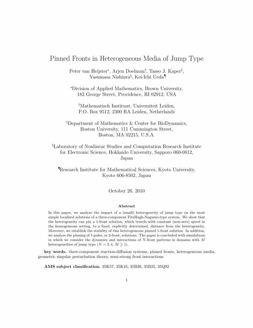
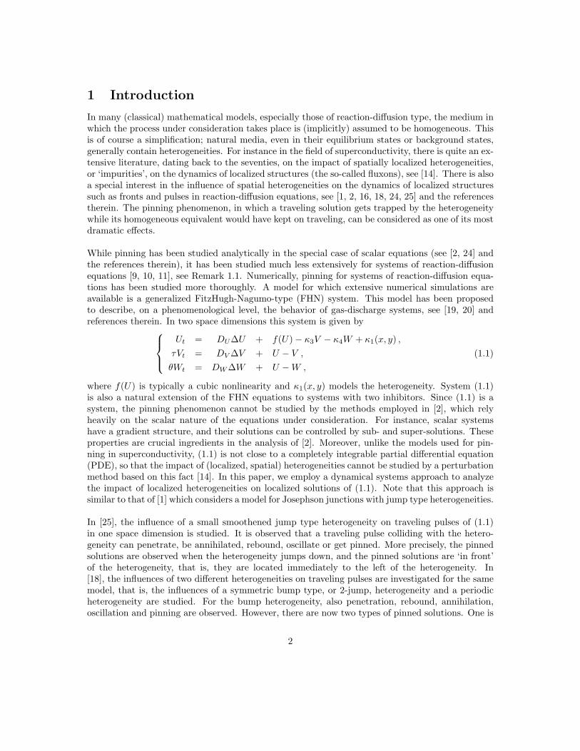
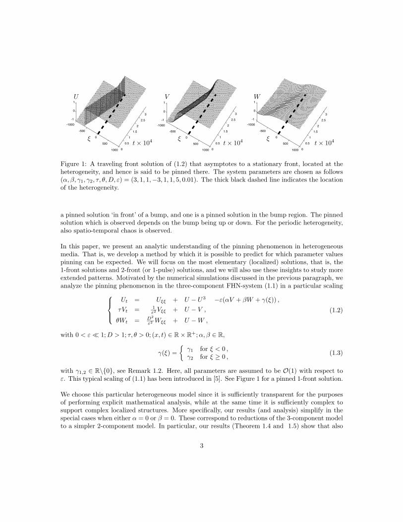
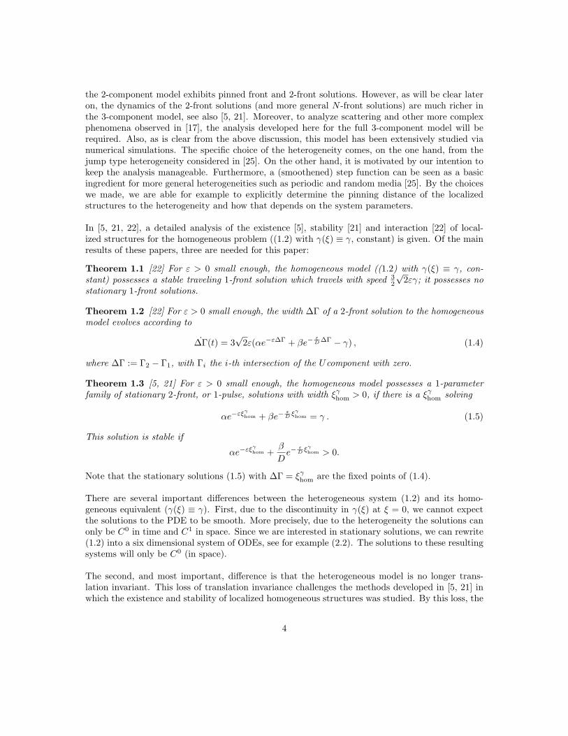
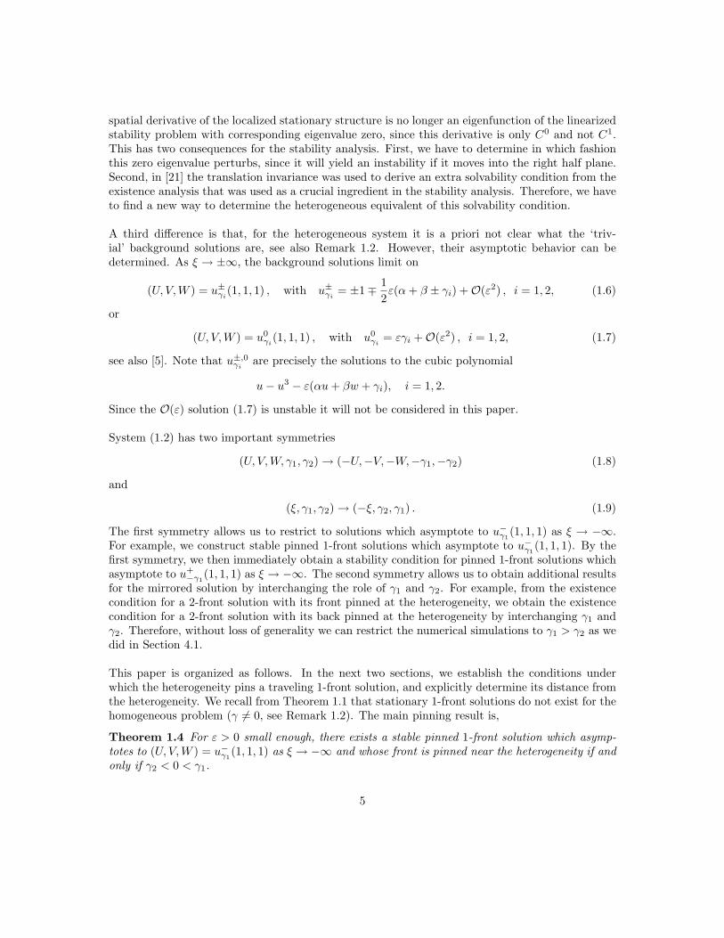
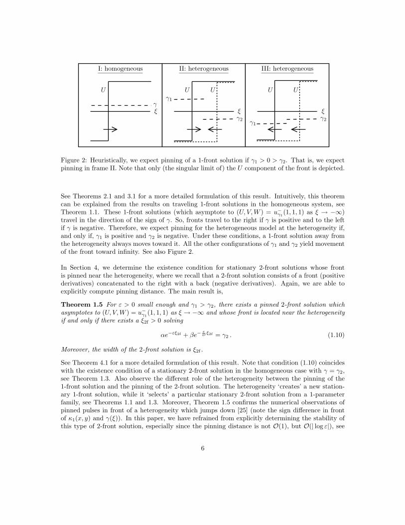
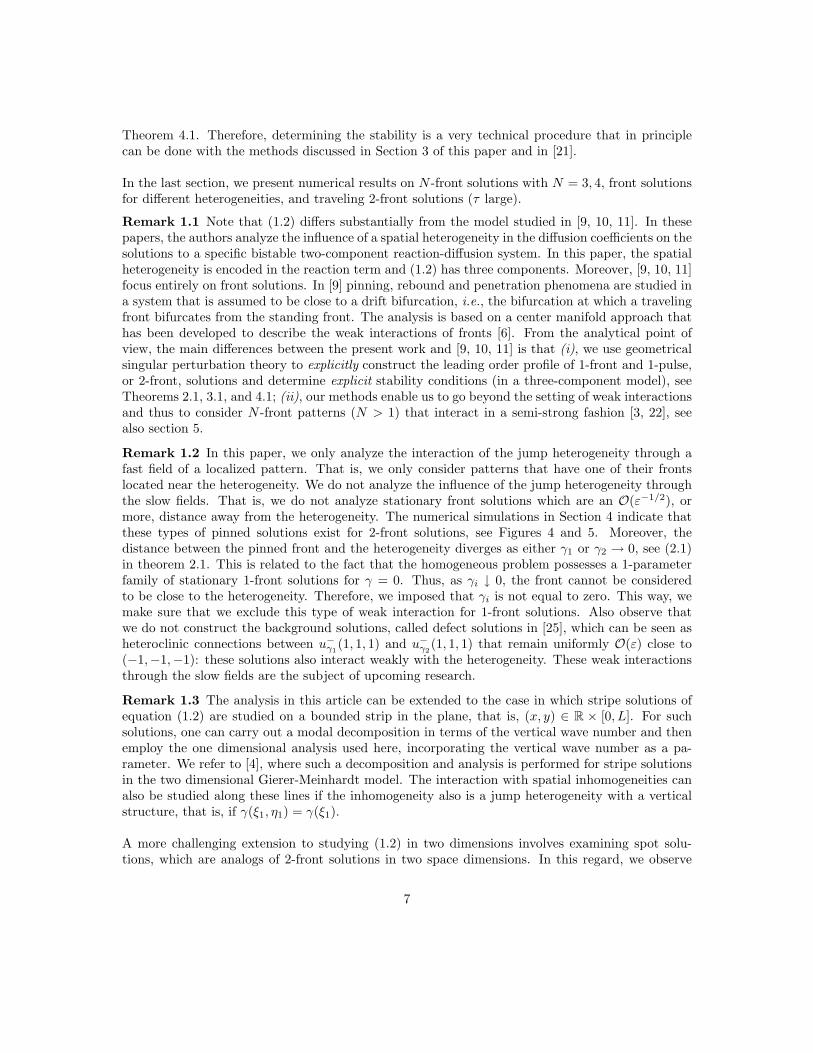
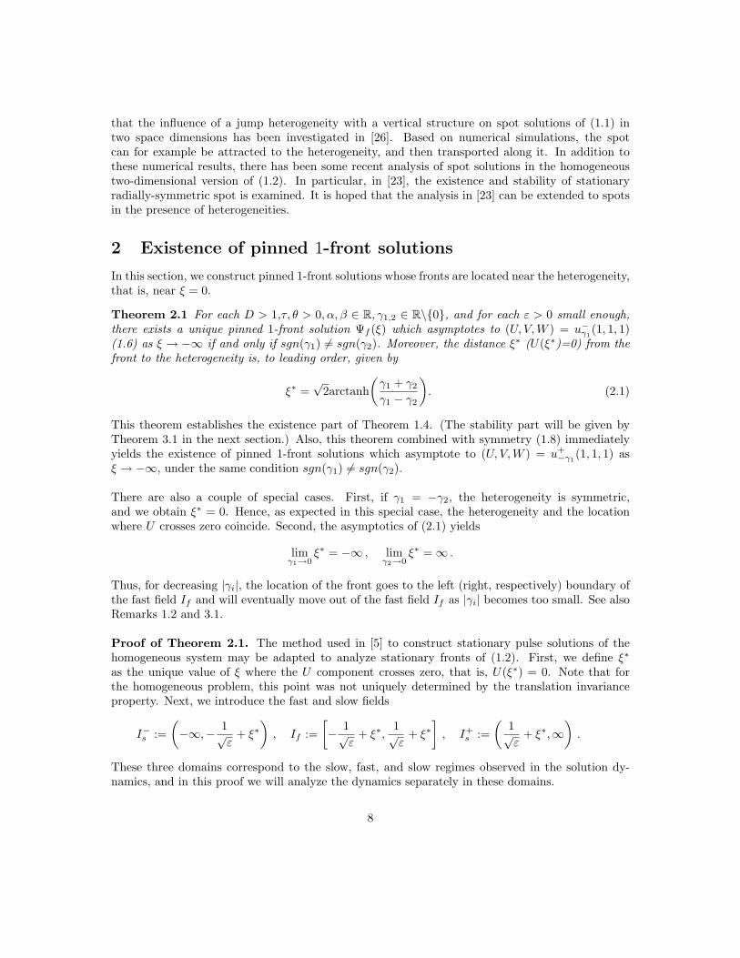
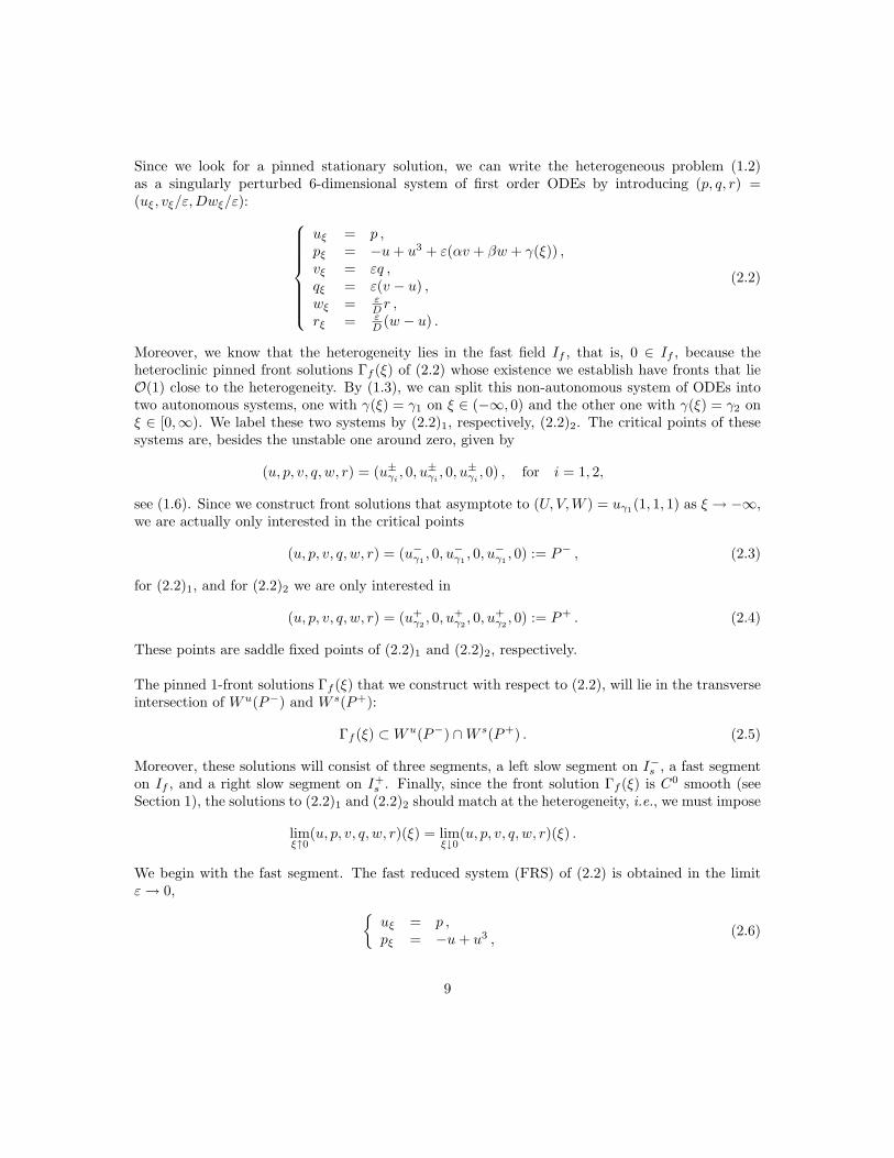
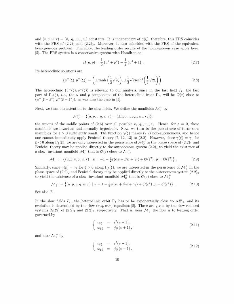
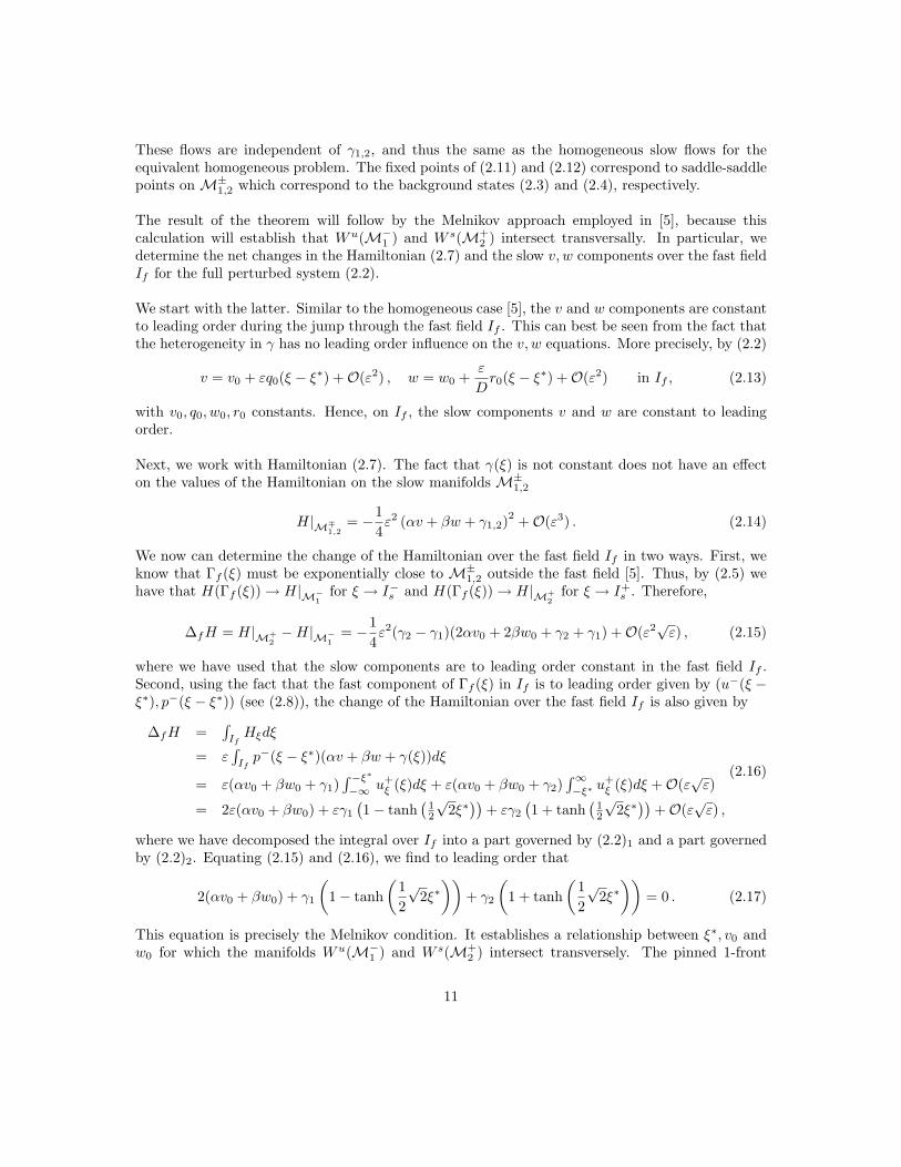
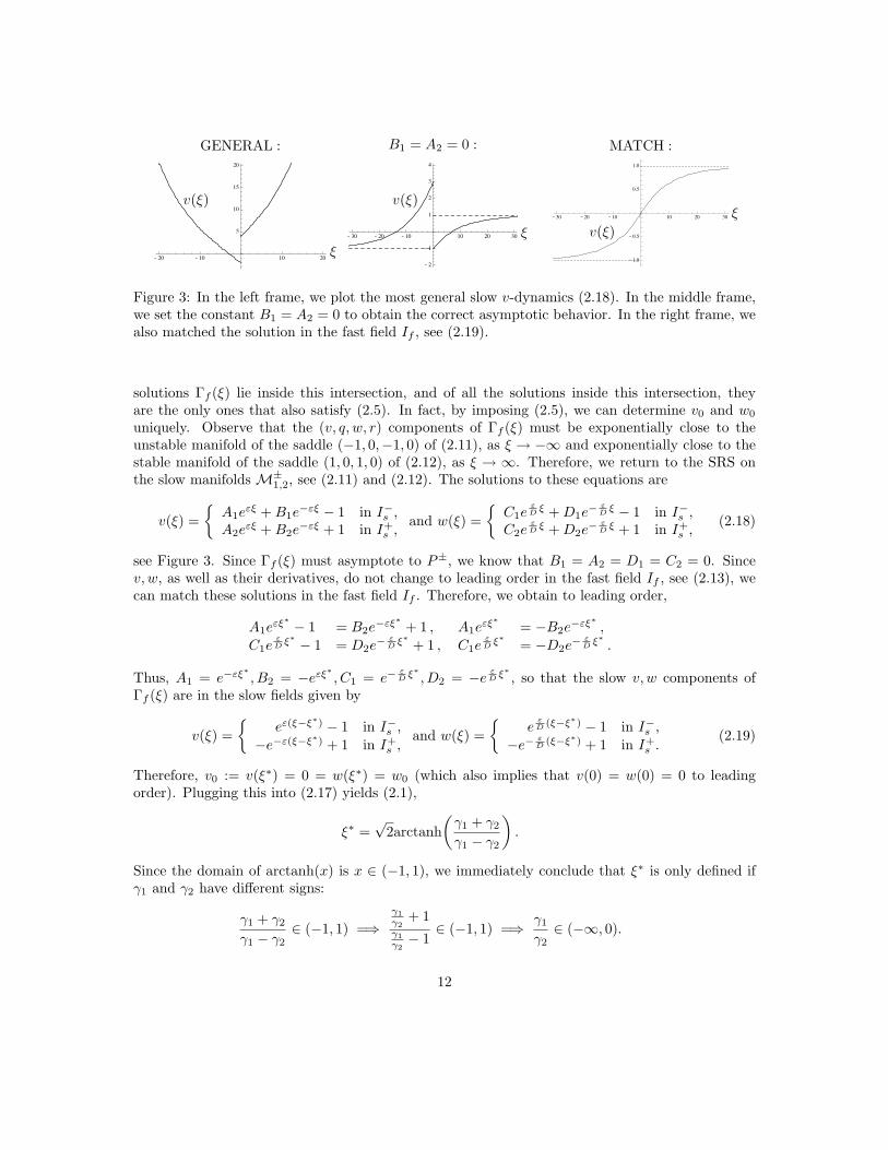


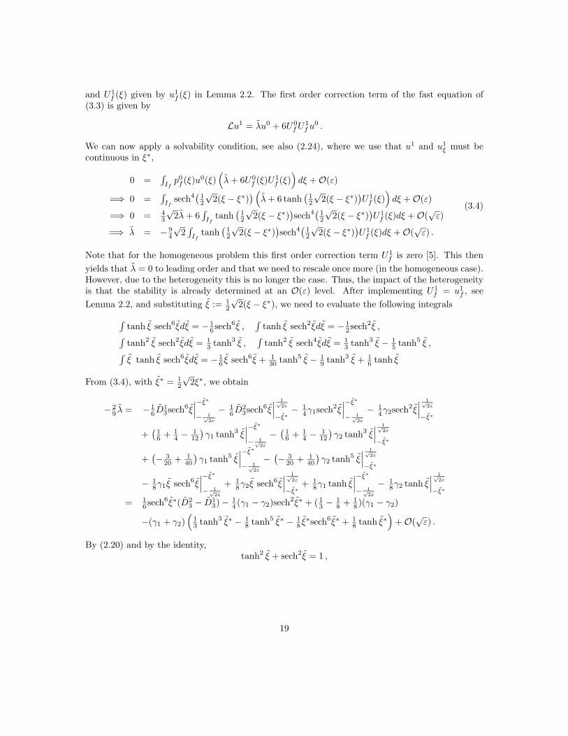
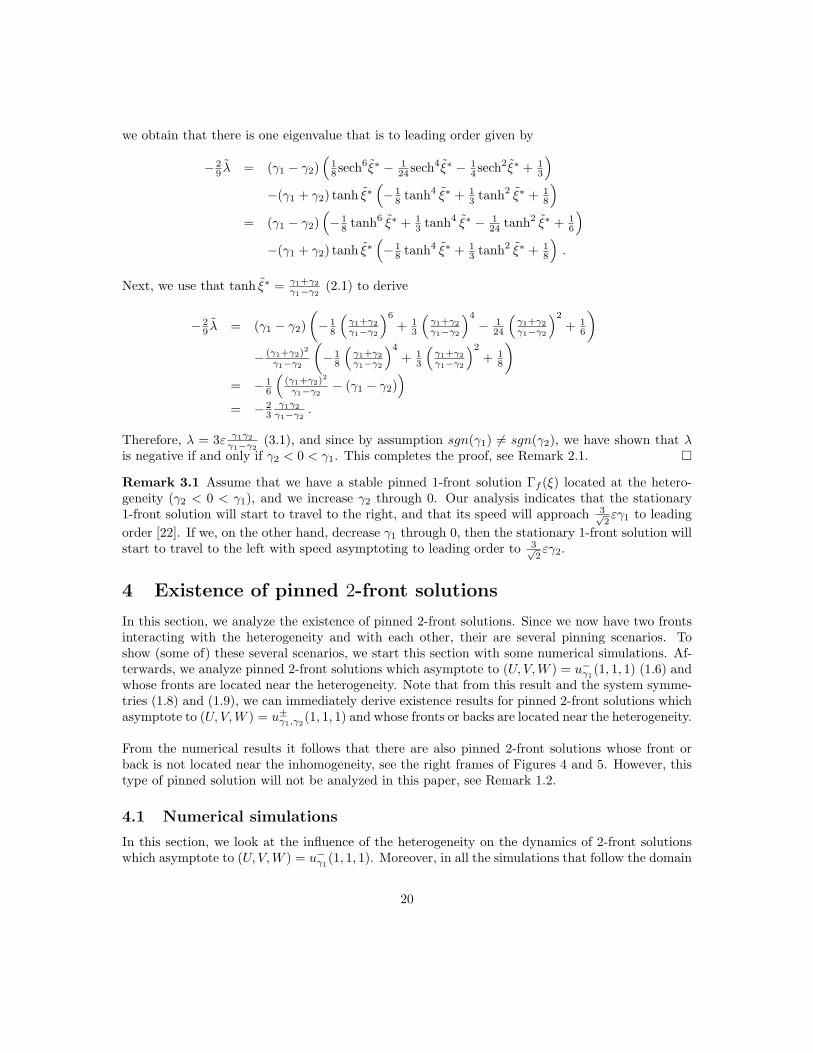
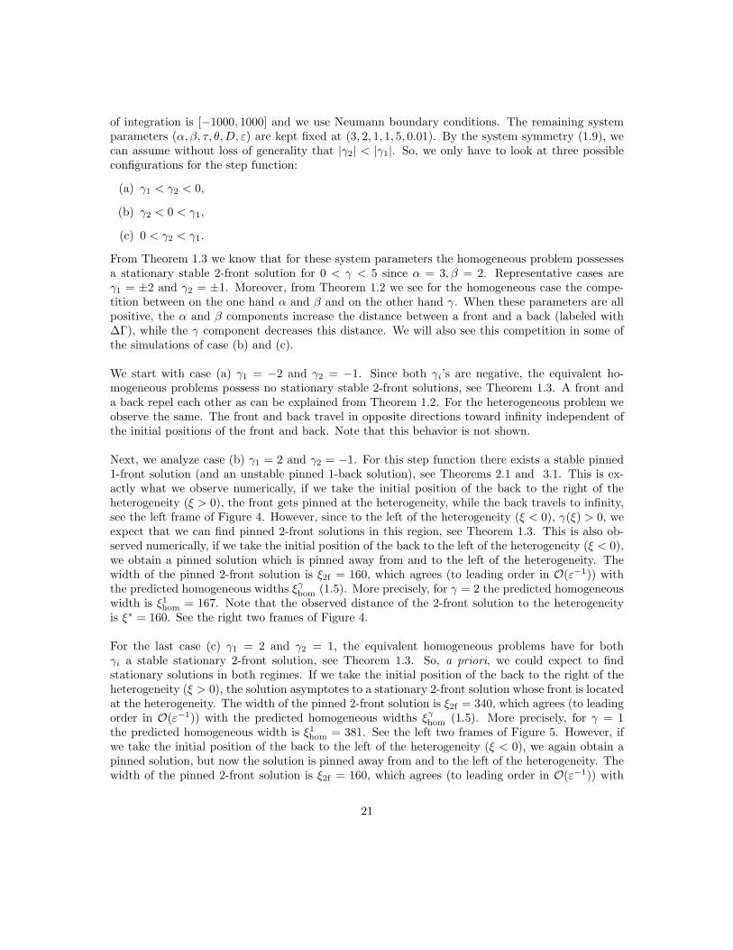
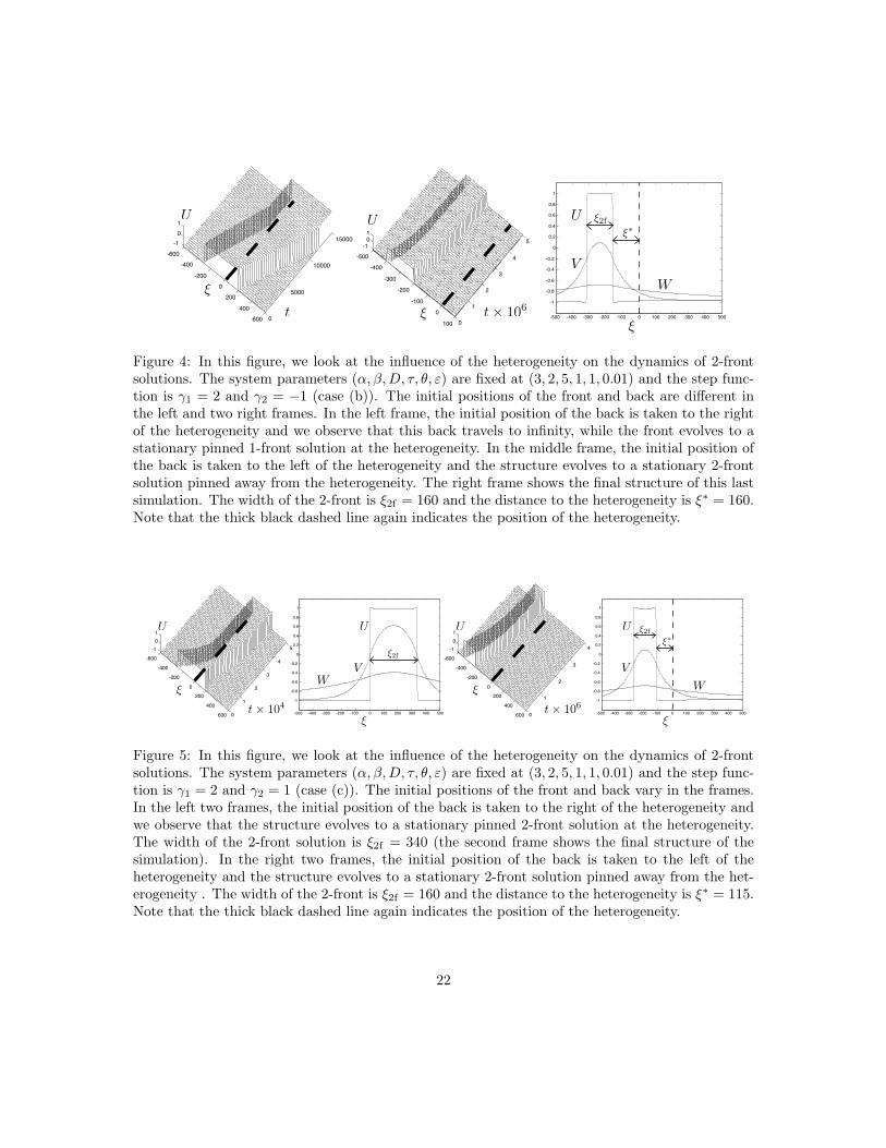

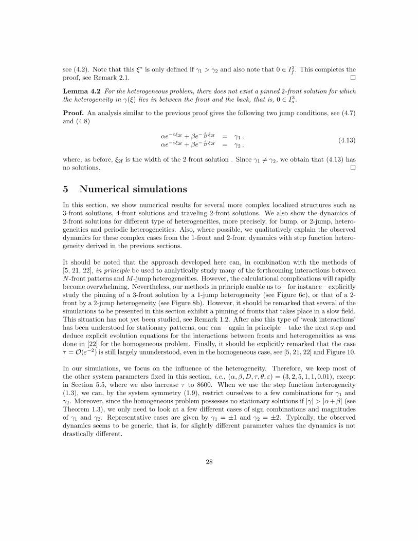
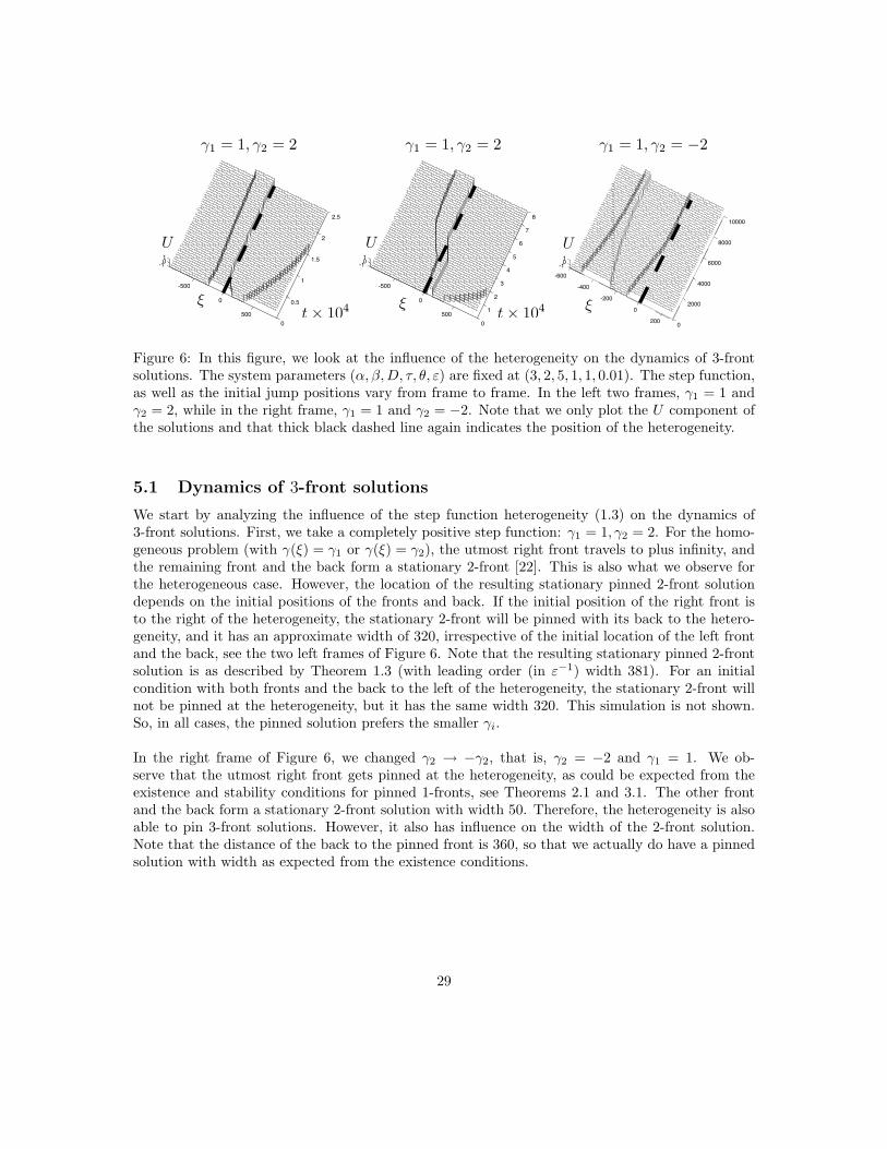
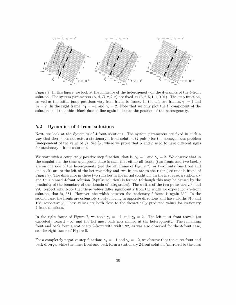
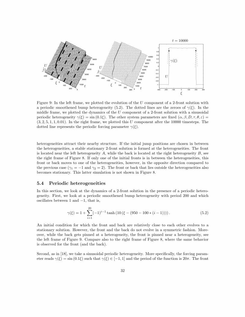

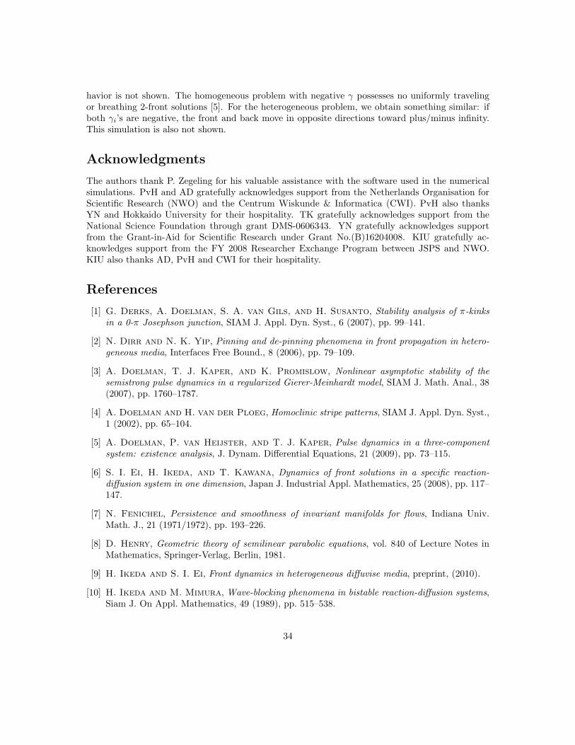


![Pinned sites in ie9 [beta]](https://static.documents.pub/doc/80x56/5554bdb8b4c90503388b4c9b/pinned-sites-in-ie9-beta.jpg)

