University of California Santa Cruz Pitch Correction for the Human Voice A thesis submitted in partial satisfaction of the requirements for the degree of Bachelor Of Science in Physics by Michael A. Peimani June 10, 2009
Transcript
University of California
Santa Cruz
Pitch Correction for the Human Voice
A thesis submitted in partial satisfactionof the requirements for the degree of
Pitch correction for musical applications is a new and extremely influential tech-nology. Since the introduction of Antares’ Auto-Tune in 1997, the music recordingindustry has been completely revolutionized by the ability to correct out of tune vo-cals. This paper examines some of the mathematical and computational techniquesbehind pitch correction. Methods of pitch estimation and pitch correction in both thetime domain and frequency domain are discussed with an emphasis on their applicationto musical singing.
1 Foreword: A Bit of Terminology
In discussing mathematics along with music it’s often easy to get lost in terminology. For this
reason, I’ve relaxed a few definitions regarding sound and singing in the body of this work.
Although the terms “pitch” and “frequency” are known to have slightly different definitions1,
for ease of discussion the two shall be used interchangeably. In addition, the complicated
process of human singing is indeed very similar to the process of speech. Throughout this
paper, then, the term “speech” may be used to mean “voiced singing,” or vice-versa.
2 Introduction and Background
Humans have been using their voices to create musical pitch for thousands of years. With
the invention of recorded sound by Thomas Edison in 1877 came the advent of musical
recordings featuring some of the world’s greatest artists. From that time on, one could
experience the mastery of great vocal works without needing to be present at the location
of the performance. As recording technology developed with the multi-track recorder, high
fidelity records became more and more available to the masses. Over time, studio engineers
developed techniques to alter sounds during the recording and mixing process. Often these
alterations were designed to make a performance sound more “real,” but were sometimes
aimed at creating new sounds which were impossible to produce without the use of modern
computers. Artificial reverb is a good example of something designed to simulate “natural
1Whereas frequency is an absolute measure of rate, pitch is a relative term used often in music to relateone note to another.
2
sound,” while the electronic synthesizer is often used for synthetic music production. Re-
cently, computer technology has made it possible to alter the sound of the recorded voice in
ways heretofore unimaginable. Many effects have been applied to recorded singing, but the
most influential by far has been the introduction of pitch-correction software.
Pitch correction is exactly what it sounds like: A vocal performance is altered by a
computer such that every note is reproduced with perfect pitch. What this means is a singer
can make a mistake in pitch during the recording process and a computer, using a variety of
algorithms, can “correct” the pitch of the fouled note. This can, in fact, be used to correct
several mistakes or even an entire performance if a singer has the tendency to sing out of
tune. What’s more, with modern computer chips this process can be done in real-time2 and
pitch can be corrected during a live performance!
This paper gives an in depth look at the computational methods behind pitch correction.
Techniques are discussed for analyzing and processing audio in both the time domain and
the frequency domain. The pitch-synchronous overlap and add method and the modified
phase vocoder are investigated in detail, and pitch detection algorithms are explained.
3 Introduction to Musical Pitch and Sound
The idea of musical pitch is directly related to the concept of frequency. The human ear can
detect sound frequencies between around 15 and 20,000 Hz. It is assumed the reader has a
basic understanding of sound waves and how they propagate through air, but it’s important
to remember that at any time, your ear is only subject to one given air pressure level. As
sound waves pass by, the air pressure at the ear changes in accordance with the wave. This
change or oscillation is what is recorded by microphones, and, eventually, encoded digitally
as a string of numbers as will be explained here in the section on Pulse-Code-Modulation.
2Here, what is meant by real-time is an imperceptible delay between the source signal input and theprocessed signal output.
3
3.1 Timbre
Another important aspect of musical sound is the idea of timbre. Timbre is a psychoacoustic
phenomenon that is best described as the “color” or “tone” of a pitch, also known as the
“character” of a sound. Timbre is what distinguishes a piano’s sound from, say, a saxo-
phone’s. Both instruments playing the same pitch (note) are easily distinguishable because
each has a unique timbre. From a technical standpoint, timbre is related to the frequency
spectrum of a sound. When an instrument produces a particular pitch, such as A4 (de-
fined to be 440Hz), a series of overtones are produced depending on the instrument and
technique used to play it. These overtones are often integer multiples of the note intended
and are what give the particular instrument its “color.” The intended note is called the
fundamental frequency and the overtones are also called harmonics. Of interest to this paper
is that the human voice also produces harmonics when singing. These harmonics are also
called “overtones,” or “formants.” Formants are, in fact, the main attributes which enable
listeners to distinguish between different singers. The concepts of fundamental frequency
and overtones are important to any pitch correction system and will be expanded upon in
the section regarding pitch-estimation.
4 Basics of Digital Audio and Spectral Analysis
4.1 Encoding digital audio - Pulse Code Modulation
Before discussing the techniques of pitch correction it’s important to have an understanding
of how sound is recorded digitally. The most basic form of digitized sound is called Pulse
Code Modulation, or PCM. Pulse Code Modulation stores an analog signal in discrete time
steps with discrete amplitudes. Whereas an analog sound wave is continuous, a computer
can only store discrete values. The digitization process goes as follows: A sound source is
recorded by a microphone, which induces a current in a wire. An analog to digital converter
(ADC) takes the incoming signal and samples it at a given frequency, Fs. Each sample is
stored as a particular value, and the next sample is taken. The number of values available
4
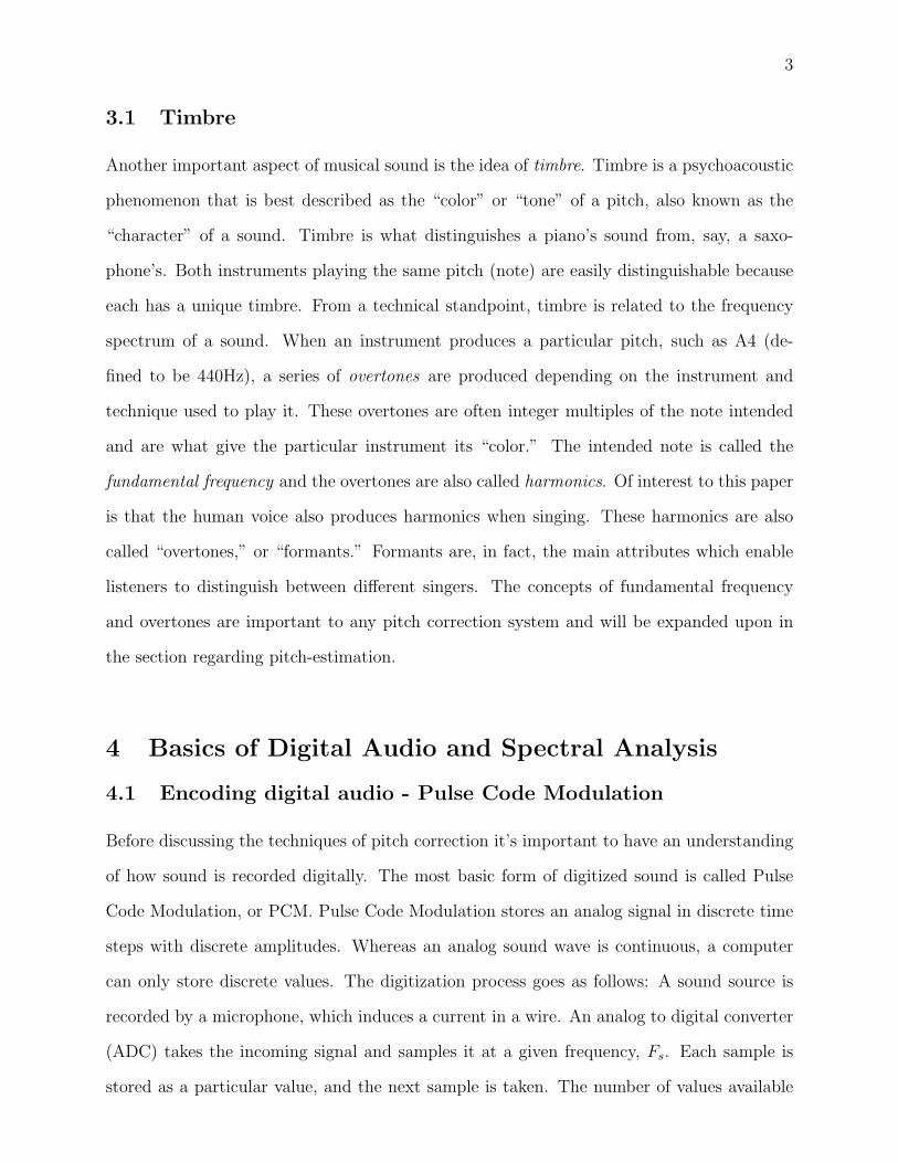
Figure 1: Illustration of quantization errors as a result of PCM encoding. Original waveformis marked by dashed line, encoded signal marked by solid line. Note the discontinuitiesin PCM waveform will translate to extremely high frequencies in the Fourier Transformfrequency spectrum, hence a low-pass filter is applied.
can be thought of as the amplitude resolution of the ADC, which depends on the ADC itself.
For example, an 8-bit ADC can store 28 = 256 different values, and a 16-bit converter can
distinguish between 216 = 65, 526 values. One can imagine the sound quality of a 16-bit ADC
to be far superior to an 8-bit chip when both are operated at the same sampling frequency.
For traditional CDs, Fs = 44, 100 Hz with 16 bits of amplitude resolution.
The inherent nature of storing audio digitally means that some approximations must be
made. The process of taking an analog signal and associating with it specific values within
the range available by the coding process is called quantization. Quantization introduces
frequency components into the recorded signal that weren’t necessarily present in the original
waveform. Because of this, signals are often processed by a low-pass filter, which filters out
the high frequency components. An illustration of a PCM waveform with quantization error
is shown in figure 1.
It should be understood now that audio stored on a computer in PCM form is essentially
a long string of values corresponding to a sequence of particular currents or voltages, with
one stored value for every 1/Fs of a second. To listen to the audio, the reverse process takes
place: The string of values is decoded by a Digital-to-Analog converter (DAC) and is output
5
as a voltage or current on a wire. This voltage can be amplified to drive a speaker, producing
the recorded sound. It’s important to realize that digital sound is stored in discrete values
to appreciate the need for the Discrete Fourier Transform.
4.2 The Discrete Fourier Transform
Fourier analysis is one of the most important mathematical techniques in signal processing.
The Fourier transform presents a way of converting a signal in the time-domain to one in
the frequency domain. That is to say: it takes a function of a real variable (time) and turns
it into a function of frequency. The Fourier transform of an audio signal often has complex
values, which are representative of amplitude and phase information. The plot of frequency
vs. the absolute value of the complex outputs of a Fourier transform can be thought of as
a power spectrum. The power spectrum is a sort of fingerprint of the original signal, as it’s
snapshot of the frequency components present in the original signal. Fourier showed that
any periodic function can be broken up into its constituent frequencies in this manner.
Since computer audio signals record amplitude at discrete time values, a technique called
the Discrete Fourier transform (DFT) is implemented to analyze digital audio[3]. The DFT
is therefore a discrete-valued version of the Fourier transform. A common form of the DFT
is found below:
x[n] ≡ x (nTs) =1
N
N−1∑k=0
X[k]ei2πkn/N , n = 0, 1, 2, ..., N − 1 (1)
X[k] ≡ FsX (kFs/N) =1
N
N−1∑n=0
x[n]e−i2πkn/N , k = 0, 1, 2, ..., N − 1 (2)
In this format, x[n] is a discrete valued function of time and can be thought of as the
original sampled audio. N is the total number of samples, Fs is the sampling frequency,
Ts = 1/Fs is the sample length, and the total signal duration is T = N × Ts. X[k] is
therefore the transform of x[n], and is a function of frequency k. The Discrete Fourier
transform is capable of resolving frequencies up to N/2 Hz.
6
4.2.1 The Fast Fourier Transform
The Fast Fourier transform, or FFT, is an implementation of the Discrete Fourier Transform.
It gets its name because of its ability to greatly reduce the number of computations needed
to perform a DFT. A DFT of N samples takes N × N = N2 complex multiplications and
additions to carry out, while a DFT reduces the problem to roughly Nlog2(N) complex
multiply-adds [3]. The great computational efficiency of the FFT led to advancements in
signal processing and the possibility of complex real-time processing3
5 Pitch Estimation Methods
5.1 Goals of a pitch estimation algorithm
The first step in altering or correcting the pitch of a voiced signal is to properly identify
the note being sounded or sung. After all, in order to shift from one frequency to another,
one must indeed know the original frequency. Determining this is no trivial task, and much
work has been done in pitch-estimation theory. Applications of pitch determination aren’t
limited to music. In fact, this type of analysis is important for all types of signal processing
and some engineering work. Pitch estimation uses any and all tools available to determine
the fundamental frequency Fs. Often, a knowledge of typical frequencies present in the
signal can help optimize pitch-estimation algorithms. In the case of musical singing, these
frequencies range from a low bass at around 80 Hz to a high soprano at 1,100 Hz, or E2 to
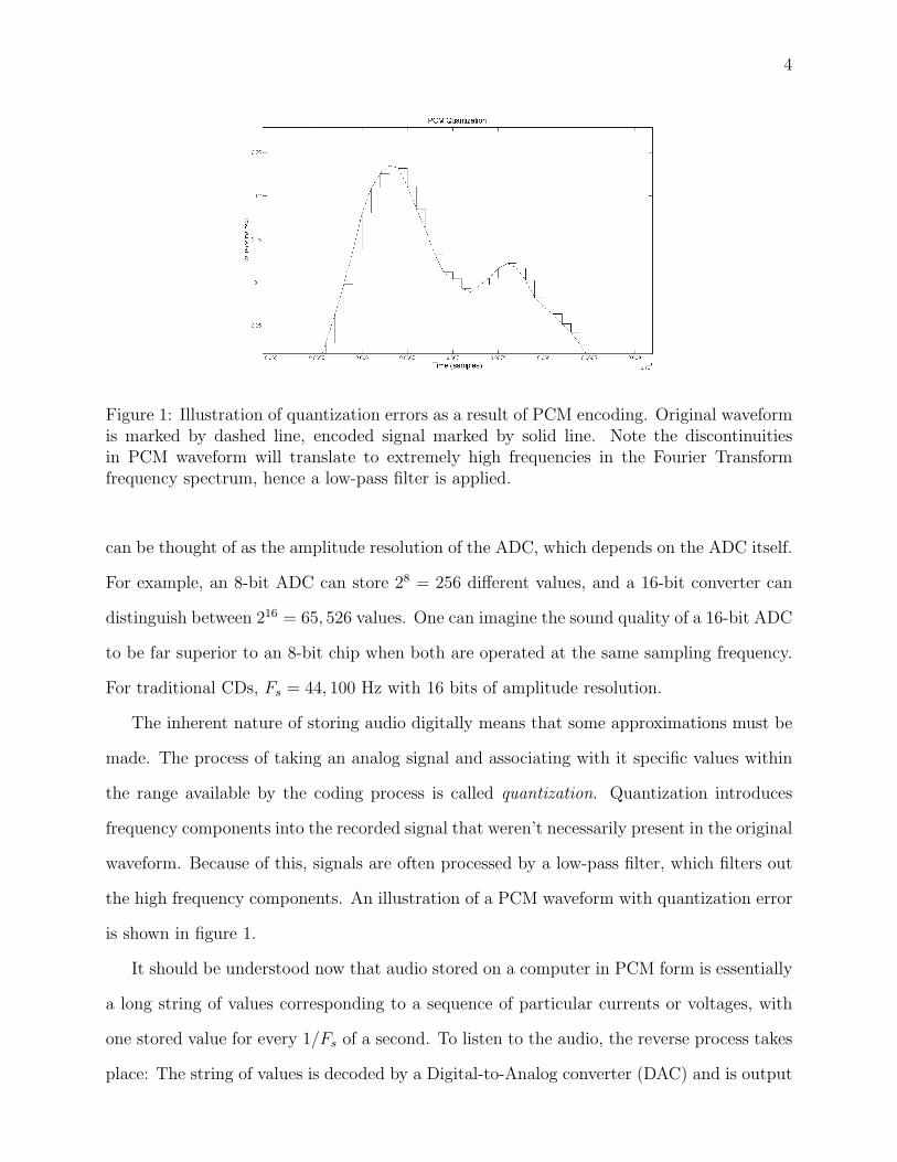
C6 on the piano. It’s important to note that a typical sampling frequency of 44.1 kHz is
more than adequate to resolve fundamentals in this range. For example, a 1,000 Hz wave
will have Fs/1, 000 ' 44 samples to represent one full period as seen in figure 2.
Of course, the human voice doesn’t produce a perfect sine wave. Instead it produces a
complex waveform which contains a fundamental frequency, F0, with a signature of harmonics
unique to the individual singer. While some of these harmonics may be outside the resolvable
range, it is the fundamental which is sought by the pitch-estimation algorithm.
3For further reading on Fast Fourier Transforms see [3] [1] or any thorough signal processing text.
7
Figure 2: 1000 Hz sine wave sampled at 44.1 kHz. Sample points are marked by ◦.
5.2 A Few Technicalities
Any pitch estimation algorithm takes a discrete signal x(n) as an input. x(n) is often
a sampled version of the original continuous signal x(t). From here on we’ll be working
primarily with the sampled signal x(n) and its discrete Fourier transform X(k). Remember
that n is the sample number, and the amount of time between successive samples is the
sample period Ts = 1/Fs. In this way, n is a time variable, so x(n) is a function of time.
As an example, a one second recording with a sampling rate of Fs =44.1 kHz will produce
44,100 total samples, which we call N = # samples. The range of n, then, is 1 < n < N .
In the frequency domain, the variable k represents individual frequencies. More precicely,
k translates to actual frequencies f in Hz as
f =kFsN
.
So X(k) gives amplitude and phase information as a function of frequency. A common way
of visualizing the transform X(k) is to plot the absolute value of X, which is a representation
of the amount of energy present at each frequency. It’s also important to note that a discrete
Fourier transform of length N samples is only capable of analyzing frequencies up to a certain
8
frequency, callded the Nyquist frequency:
fNy =1
2
kFsN
.
This is due to the fact that frequencies from fNy to 2fNy in the transform are actually
reflections of frequencies in the range 0 < f < fNy. The Nyquist frequency is usually half
the sampling rate, fNy = Fs/2 and is a fundamental property of sampling theory. The idea
is that the highest frequency one can digitally encode given a certain sampling rate is a
signal oscillating at half that rate [10].
5.3 Windowing
One of the most fundamental processes in signal processing is the breaking up of a discretely
sampled signal into smaller constituents or “windows.” In the context of pitch-correction,
windows are analyzed and processed individually, then recombined to produce a coherent
output. For example, to determine the pitch of a particular vocal passage, the signal is di-
vided into windows of lengths on the order of a few pitch-cycles. The fundamental frequency
of each window is then found and used to process the final output. The most simple method
of windowing, as it’s called, is to take the samples exactly as they are in the original and
divide them into groups. This can be thought of as multiplying the signal by a rectangular
windowing function:
w(n) =
1 , 0 < n < N
0 , elsewhere,
where n is the sample number, and N is the total number of samples per window (window
size). The problem with this type of window involves advanced topics in Fourier analysis,
but can be summarized by saying that the transform of a signal windowed by the function
above will contain energy at frequencies not actually present in the original signal [3]. In
fact, any window function will introduce new frequency components to a windowed signal.
9
The goal, then, is to use a window function which minimizes these effects.
One useful window is the Hamming window, defined by:
wH(n) = 0.54 + 0.46 cos(
2πN
N − 1
),
offers reasonable results for our application. In the process of dividing up the original signal
into smaller pieces, then, a window function is usually applied as x(n)w(n).
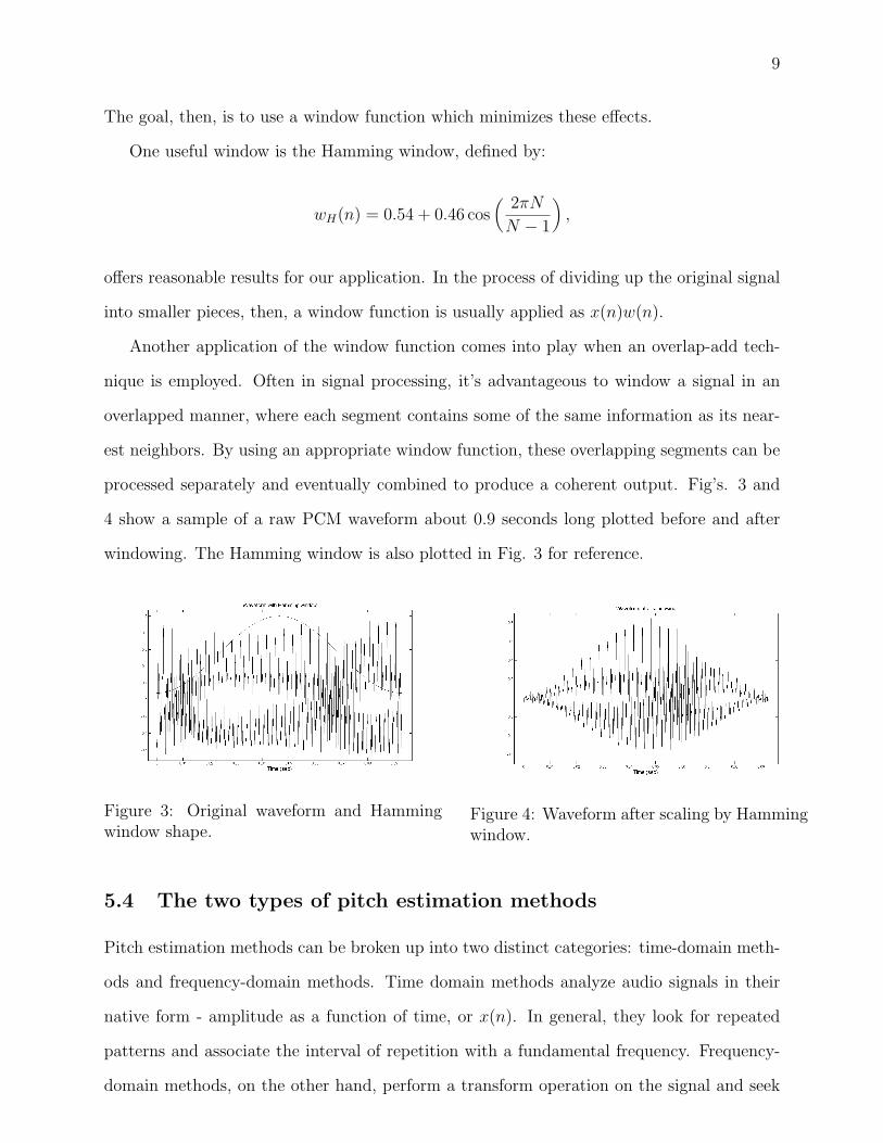
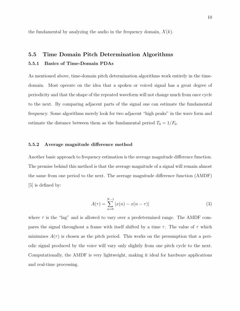
Another application of the window function comes into play when an overlap-add tech-
nique is employed. Often in signal processing, it’s advantageous to window a signal in an
overlapped manner, where each segment contains some of the same information as its near-
est neighbors. By using an appropriate window function, these overlapping segments can be
processed separately and eventually combined to produce a coherent output. Fig’s. 3 and
4 show a sample of a raw PCM waveform about 0.9 seconds long plotted before and after
windowing. The Hamming window is also plotted in Fig. 3 for reference.
Figure 3: Original waveform and Hammingwindow shape.
Figure 4: Waveform after scaling by Hammingwindow.
5.4 The two types of pitch estimation methods
Pitch estimation methods can be broken up into two distinct categories: time-domain meth-
ods and frequency-domain methods. Time domain methods analyze audio signals in their
native form - amplitude as a function of time, or x(n). In general, they look for repeated
patterns and associate the interval of repetition with a fundamental frequency. Frequency-
domain methods, on the other hand, perform a transform operation on the signal and seek
10
the fundamental by analyzing the audio in the frequency domain, X(k).
5.5 Time Domain Pitch Determination Algorithms
5.5.1 Basics of Time-Domain PDAs
As mentioned above, time-domain pitch determination algorithms work entirely in the time-
domain. Most operate on the idea that a spoken or voiced signal has a great degree of
periodicity and that the shape of the repeated waveform will not change much from once cycle
to the next. By comparing adjacent parts of the signal one can estimate the fundamental
frequency. Some algorithms merely look for two adjacent “high peaks” in the wave form and
estimate the distance between them as the fundamental period T0 = 1/F0.
5.5.2 Average magnitude difference method
Another basic approach to frequency estimation is the average magnitude difference function.
The premise behind this method is that the average magnitude of a signal will remain almost
the same from one period to the next. The average magnitude difference function (AMDF)
[5] is defined by:
A(τ) =N−1∑n=0
|x(n)− x(n− τ)| (3)
where τ is the “lag” and is allowed to vary over a predetermined range. The AMDF com-
pares the signal throughout a frame with itself shifted by a time τ . The value of τ which
minimizes A(τ) is chosen as the pitch period. This works on the presumption that a peri-
odic signal produced by the voice will vary only slightly from one pitch cycle to the next.
Computationally, the AMDF is very lightweight, making it ideal for hardware applications
and real-time processing.
11
5.5.3 Autocorrelation Method
The autocorrelation method is similar to the AMDF in that it finds the period T0 by compar-
ing the waveform with itself shifted by a time τ . The difference being a more sophisticated
method of comparison. The derivation of the normalized autocorrelation function is well
explained in [5], while a summarized version is presented here. A basic method of comparing
two waveforms is called the direct distance method:
E(τ) =1
N
N−1∑n=0
[x(n)− x(n+ τ)]2.
Similarly to the AMDF, the value of τ which minimizes the error E(τ) is chosen as the
fundamental period T0. This technique works well, but often fails at portions of speech with
quickly varying energy levels, such as at speech onsets and offsets. To compensate for this,
a scaling factor β is introduced:
E(τ) =1
N
N−1∑n=0
[x(n)− βx(n+ τ)]2.
β is found by setting δE(τ, β)/δ(β) = 0 [5]. With this new factor defined, the error becomes:
E(τ, β) =N−1∑n=0
x2(n)−R2n(τ)
where
R2n(τ) =
[∑N−1n=0 x(n)x(n+ τ)
]2∑N−1n=0 x
2(n+ τ).
Minimizing E(τ, β) is then the equivalent of maximizing R2n(τ). As one last detail, the square
root of R2n(τ) is taken to avoid possible maxima where the correlation is in fact negative.
The result is therefore:
Rn(τ) =
∑N−1n=0 x(n)x(n+ τ)√∑N−1
n=0 x2(n+ τ)
.
Again, the value of τ which maximizes Rn(τ) is chosen as the fundamental period. This pe-
12
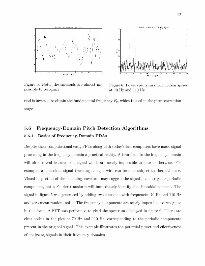
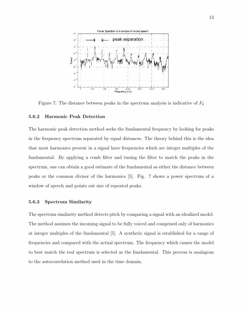
Figure 5: Note: the sinusoids are almost im-possible to recognize.
Figure 6: Power spectrum showing clear spikesat 70 Hz and 110 Hz.
riod is inverted to obtain the fundamental frequency F0, which is used in the pitch-correction
stage.
5.6 Frequency-Domain Pitch Detection Algorithms
5.6.1 Basics of Frequency-Domain PDAs
Despite their computational cost, FFTs along with today’s fast computers have made signal
processing in the frequency domain a practical reality. A transform to the frequency domain
will often reveal features of a signal which are nearly impossible to detect otherwise. For
example, a sinusoidal signal traveling along a wire can become subject to thermal noise.
Visual inspection of the incoming waveform may suggest the signal has no regular periodic
component, but a Fourier transform will immediately identify the sinusoidal element. The
signal in figure 5 was generated by adding two sinusoids with frequencies 70 Hz and 110 Hz
and zero-mean random noise. The frequency components are nearly impossible to recognize
in this form. A FFT was performed to yield the spectrum displayed in figure 6. There are
clear spikes in the plot at 70 Hz and 110 Hz, corresponding to the periodic components
present in the original signal. This example illustrates the potential power and effectiveness
of analyzing signals in their frequency domains.
13
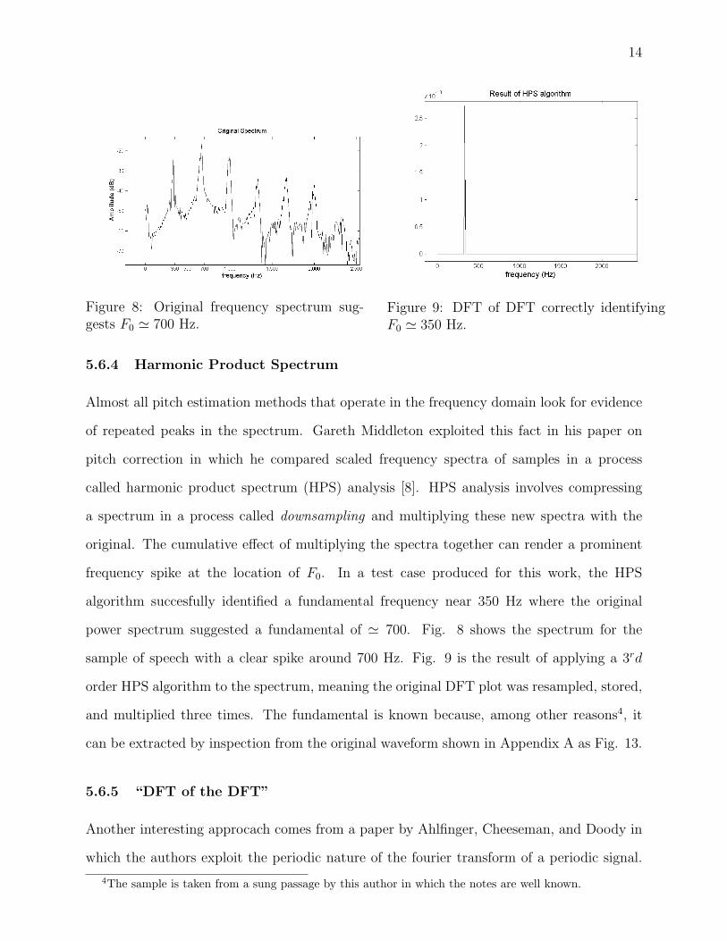
Figure 7: The distance between peaks in the spectrum analysis is indicative of F0
5.6.2 Harmonic Peak Detection
The harmonic peak detection method seeks the fundamental frequency by looking for peaks
in the frequency spectrum separated by equal distances. The theory behind this is the idea
that most harmonics present in a signal have frequencies which are integer multiples of the
fundamental. By applying a comb filter and tuning the filter to match the peaks in the
spectrum, one can obtain a good estimate of the fundamental as either the distance between
peaks or the common divisor of the harmonics [5]. Fig. 7 shows a power spectrum of a
window of speech and points out size of repeated peaks.
5.6.3 Spectrum Similarity
The spectrum similarity method detects pitch by comparing a signal with an idealized model.
The method assumes the incoming signal to be fully voiced and comprised only of harmonics
at integer multiples of the fundamental [5]. A synthetic signal is established for a range of
frequencies and compared with the actual spectrum. The frequency which causes the model
to best match the real spectrum is selected as the fundamental. This process is analagous
to the autocorrelation method used in the time domain.
14
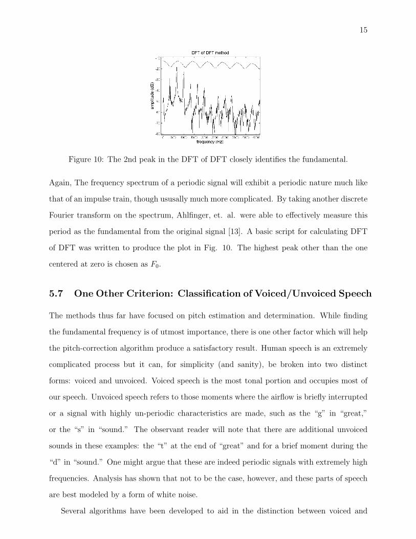
Figure 8: Original frequency spectrum sug-gests F0 ' 700 Hz.
Figure 9: DFT of DFT correctly identifyingF0 ' 350 Hz.
5.6.4 Harmonic Product Spectrum
Almost all pitch estimation methods that operate in the frequency domain look for evidence
of repeated peaks in the spectrum. Gareth Middleton exploited this fact in his paper on
pitch correction in which he compared scaled frequency spectra of samples in a process
a spectrum in a process called downsampling and multiplying these new spectra with the
original. The cumulative effect of multiplying the spectra together can render a prominent
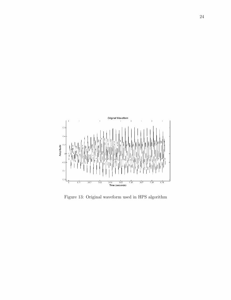
frequency spike at the location of F0. In a test case produced for this work, the HPS
algorithm succesfully identified a fundamental frequency near 350 Hz where the original
power spectrum suggested a fundamental of ' 700. Fig. 8 shows the spectrum for the
sample of speech with a clear spike around 700 Hz. Fig. 9 is the result of applying a 3rd
order HPS algorithm to the spectrum, meaning the original DFT plot was resampled, stored,
and multiplied three times. The fundamental is known because, among other reasons4, it
can be extracted by inspection from the original waveform shown in Appendix A as Fig. 13.
5.6.5 “DFT of the DFT”
Another interesting approcach comes from a paper by Ahlfinger, Cheeseman, and Doody in
which the authors exploit the periodic nature of the fourier transform of a periodic signal.
4The sample is taken from a sung passage by this author in which the notes are well known.
15
Figure 10: The 2nd peak in the DFT of DFT closely identifies the fundamental.
Again, The frequency spectrum of a periodic signal will exhibit a periodic nature much like
that of an impulse train, though ususally much more complicated. By taking another discrete
Fourier transform on the spectrum, Ahlfinger, et. al. were able to effectively measure this
period as the fundamental from the original signal [13]. A basic script for calculating DFT
of DFT was written to produce the plot in Fig. 10. The highest peak other than the one
centered at zero is chosen as F0.
5.7 One Other Criterion: Classification of Voiced/Unvoiced Speech
The methods thus far have focused on pitch estimation and determination. While finding
the fundamental frequency is of utmost importance, there is one other factor which will help
the pitch-correction algorithm produce a satisfactory result. Human speech is an extremely
complicated process but it can, for simplicity (and sanity), be broken into two distinct
forms: voiced and unvoiced. Voiced speech is the most tonal portion and occupies most of
our speech. Unvoiced speech refers to those moments where the airflow is briefly interrupted
or a signal with highly un-periodic characteristics are made, such as the “g” in “great,”
or the “s” in “sound.” The observant reader will note that there are additional unvoiced
sounds in these examples: the “t” at the end of “great” and for a brief moment during the
“d” in “sound.” One might argue that these are indeed periodic signals with extremely high
frequencies. Analysis has shown that not to be the case, however, and these parts of speech
are best modeled by a form of white noise.
Several algorithms have been developed to aid in the distinction between voiced and
16
unvoiced sounds. For a good overview see Digital Speech by A. Kondoz [5]. The most
basic of these looks for the general feature of periodicity in a signal. It is similar to the
autocorrelation method discussed before, but in this case a threshold is set. Any window of
signal which doesn’t exhibit enough periodicity is determined to be unvoiced. In most pitch
correction schemes unvoiced portions of the signal are left unaltered, while voiced parts are
processed and re-synthesized.
6 Pitch Correction
6.1 Concepts of Pitch correction
The end-goal of all the above pitch estimation methods was to determine the fundamental
frequency of voiced speech. Once this frequency is known, it can be used to accurately
alter the pitch of the signal. Here it should be explained that most Western music uses
what is called the equal temperament scale. This scale determines the pitches found on a
piano keyboard, and is the result of many mathematicians’ and musicians’ work from the
1500’s on [11]. For the purposes of this study it needs only be known that there are a set
of predetermined notes which are considered “in-tune” for most music. As an example, the
notes labeled C2 and C#2 have frequencies 65.4064 Hz and 69.2957 Hz, respectively. If a
cello played a note with a fundamental frequency of, say, 67.0 Hz, it would be considered
“out of tune” since it isn’t one of the allowed frequencies5. The same would go if a singer
attempting to sing C#2 made a note with fundamental frequency 67 Hz. His or her note
would be described as “flat” because it has a frequency F0 that is less than the desired pitch.
On the other hand, if the attempted note were C2 = 65.4064 Hz, the 67 Hz pitch produced
by the singer would be considered “sharp.” The purpose of a pitch correction system, then, is
to confine a singer’s pitches to a set of predetermined “allowed” notes (frequencies), thereby
making him or her always sound “in-tune.”
Just as there are methods of determining fundamental frequency in both the time-domain
567 Hz isn’t allowed because there are no established notes between C2 and C#2. There are exceptionsto the rule, but they are ignored for simplicity in this study.
17
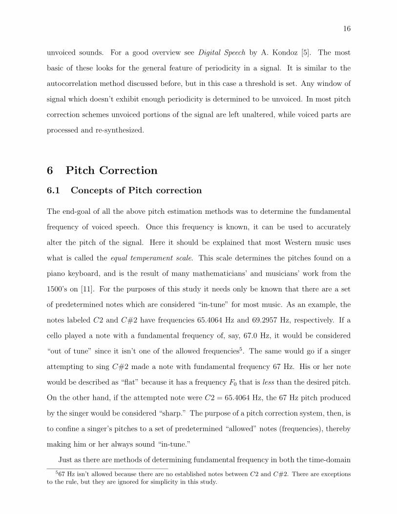
Figure 11: A rough diagram of wavelength shortening (pitch increase) by PSOLA
and frequency-domain, so, too are there methods of correcting frequency in both domains.
Both approaches have their merits and pitfalls as they are summarized below.
6.2 Time-Domain Pitch Correction
6.2.1 Pitch Synchronous Overlap Add
One very basic way of altering pitch is to play a sequence back at a different rate than it
was recorded. For example, playing a 44.1 kHz file back at twice the rate, 88.2 kHz, will
result in all pitches being doubled. The main problem with this method is that by effectively
stretching or compressing the entire signal all the harmonics and formants of the voice also
become affected. What this means in practice, is that an upward shift in frequency will result
in a so-called “chipmunk effect” in which the singer sounds much different than he would
if he were actually singing the higher note. The Pitch Synchronous Overlap-Add method
(PSOLA) is an effective and computationally efficient algorithm which preserves the singer’s
natural harmonics.
The principle of the PSOLA method is to lengthen or shorten the waveform at a very
small scale - often on the order of fractions of a period per few periods. The process goes as
follows: The original signal is analyzed by a pitch-detection algorithm and the fundamental
frequency of each window is established. Next, the waveform is given pitch-markers at
intervals equal to the pitch period T0. The markers are often placed at locations of the
largest peak in each cycle. Next, a new sequence of markers is established based on the
18
desired (target) frequencies. The synthesis process then involves matching the frequency
markers in the sampled signal with the target markers. The original signal is then windowed,
centering around every 2nd or every 4th marker, and each overlapped segment is added to the
previous one to reconstruct a full signal with the new fundamental period (see Fig. 11 for a
graphical depiction of this process) Any portion of the pitch deemed as unvoiced is simply
copied directly with no modification. Note that while the traditional window size for pitch
detection is around 90 ms long (4096 samples for 44.1 kHz audio), the windows used for
synthesis in PSOLA are much smaller: For a 300 Hz fundamental frequency, four periods is
equal to 4/300 ' 13.3ms. The method of PSOLA thus corrects pitch while preserving most
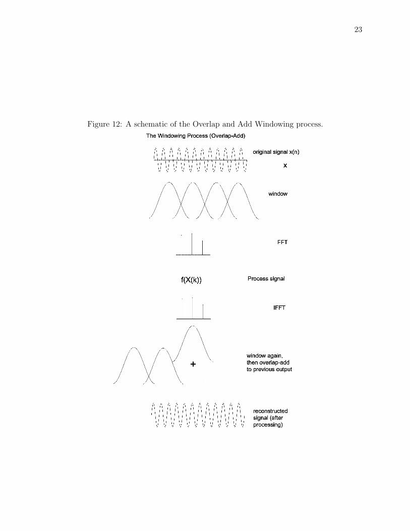
of the shape of the original waveform. Fig. 12 in the appendix shows a graphical timeline
The most promising and effective pitch modification technique which operates in the fre-
quency domain is called the modified phase vocoder. The term “vocoder” is short for “voice-
encoder,” as the original vocoder was designed in the 1930’s to transmit secure communica-
tions. The modified phase vocoder is an expansion on the original concepts and is usually
implemented digitally.
The analysis and synthesis process in the modified phase vocoder is as follows: A pitch
detection algorithm divides the original signal into overlapping segments and stores the fun-
damental frequency for each in memory. The segments are then windowed and transformed
by a FFT algorithm. The results of each transform are stored in a new matrix. A typical
design would place the output for each frequency k in the transformed function along a
column vector, with each column representing an individual window. The spectrum for each
bin is then processed individually. An algorithm then detects all the peaks present in the
frequency spectrum and shifts them by an appropriate factor - in effect altering the pitch
of each window. The scaling factor is determined by the original detected frequency and
the target frequency. A complex phasor is then multiplied to each peak and its surround-
19
ing region in order to preserve phase relationships across windows. Lastly, each column
vector is overlap-added in a reconstruction process which produces the pitch shifted signal
[2]MiddletonFrequency.
One great advantage of the modified phase vocoder is the ability to process polyphonic
signals. Polyphonic signals contain more than one fundamental frequency, such as a chord
played on a piano or the sound produced by two singers in harmony. In theory, the vocoder
could correct one out-of-tune singer and leave the other’s signal nearly unchanged. This has
huge applications when applied to live sound recordings, which are often limited to a single
stereo mix. The merits of this have yet to be seen in practice, but new technology from
Celemony promises to do exactly this [14].
7 Comments and the Future of Pitch Correction
Any musician will tell you that perfect pitch is merely a theoretical limit - that no human
can possibly sing with perfect pitch. Sure, some greats may come close, but the physiology
of the human vocal tract makes it virtually impossible to sing without a single deviation in
pitch. In some performances deviation from perfect pitch is even desired and can be used for
emphasis, tension, or style in the music. The definitive piece of software in the world of pitch
correction is “Auto-Tune,” by Antares Technologies. Auto-Tune puts accurate, high quality
pitch correction at recording engineers’ fingertips with an easy to use interface and the ability
to run on most computers. Since its introduction in 1997, Auto-Tune has revolutionized the
music industry. It has sparked an ongoing debate which divides some of the world’s top
musicians and producers. On one side of the argument is the case that pitch correction is
a form of cheating, in that it allows less-than-adequate singers to sound as if they have real
talent. The other side argues the technology has provided greater workflow in the studio,
greater records overall, and has allowed creative singers of all skill levels to present their
music in a palatable form. The debate continues, but one thing is for sure: it’s changed the
way music is made.
20
I had the privilege of interviewing Antares’ founder and chief scientist, Dr. Andy Hilde-
brand, and asked him about the direction of his technology. As the person responsible for
Auto-Tune, Dr. Hildebrand feels a sense of satisfaction that he’s completely altered the mu-
sic industry. He doesn’t forsee the immediate direction the technology will go, and admitted
he had no idea the software would be used as a voice-altering effect as it often is today6.
When asked about some of the criticism aimed at pitch correction, he kindly responded, “I’m
an engineer, not an artist,” suggesting that his goal was to write the software, not debate
its use.
One other note of interest was Dr. Hildebrand’s approach toward entrepeneurship. He
earned his PhD. in electrical engineering and has years of experience with signal processing,
from geophysics research in the oil industry to fixing sour notes in recording studios every-
where. He says some of best technology comes from innovators who see a goal and develop a
means to that end. Auto-Tune, as it turns out, processes signals entirely in the time-domain.
Dr. Hildebrand says this is the most computationally efficient method and is the reason his
products are the only pitch-correctors that work in real-time for live applications.
8 Conclusion
This work presented an investigation into the methods behind pitch correction for the human
voice. It isn’t immediately obvious whether time-domain or frequency-domain algorithms
are more effective. The general consensus in industry is to use whichever approach best suits
the needs of a particular implementation. It’s understandable to note that effective pitch
correction suitable for music applications has only become available over the last ten years.
With this in mind, it’s exciting to imagine where the technology will be in another ten.
Antares is in currently in development of an Auto-Tune based application for the iPhone,
which will make the technology available-at least on a rudimentary level-to a growing portion
of the population [4]. As computers become cheaper, we will soon find a day when advanced
6Auto-Tune is designed to transparently correct pitch, but with certain parameter settings can producean artificial vocal sound, popular in much of today’s music.
21
pitch correction can even be found in children’s toys.
References
[1] Kihong Shin, Joseph Kenneth Hammond, Fundamentals of signal processing for soundand vibration engineers. John Wiley & Sons Ltd., West Sussex, England, 2008.
[2] Jean Laroche and Mark Dolson, New phase-vocoder techniques for pitch-shifting, har-monizing, and other exotic effects, Proc. IEEE Workshop on Applications of SignalProcessing to Audio and Acoustics, New Paltz, New York, October 17-20, 1999.
[3] Marina Bosi, Richard E. Goldberg, Introduction to digital audio coding and standards.Kluwer Academic Publishers, Norwell, Massachusetts, 2003.
[4] Andy Hildebrand, Personal interview, Antares Technologies, Scotts Valley, CA, June5, 2009.
[5] A. M. Kondoz, Digital Speech - Coding for low bit rate communication systems JohnWiley & Sons Ltd., West Sussex, England, 2004.
[6] Gareth Middleton, Examples and Code, Connexions, December 17, 2003,http://cnx.org/content/m11716/1.3/.
[7] Gareth Middleton, Time Domain Pitch Correction, Connexions, December 17, 2003,http://cnx.org/content/m11711/1.3/.
[8] Gareth Middleton, Frequency Domain Pitch Correction, Connexions, December 17,2003, http://cnx.org/content/m11715/1.2/.
[9] David Gerhard, Pitch Extraction and Fundamental Frequency: History and CurrentTechniques Technical Report TR=CS 2003-06 University of Regina Saskatchewan,Canada.
[10] John Strawn, Digital Audio Signal Processing: An Anthology, A-R Editions, Inc.,Madison, WI, 1985.
[11] Stuart Isacoff, Temperament: How music became a battleground for the great mindsof western civilization, Vintage Books, a division of Random House, Inc., New York,NY, 2001, 2003.
[12] Sami Lemmetty Review of Speech Synthesis Technology, M.S. Thesis, Helsinki Uni-versity of Technology, Department of Electrical and Communications Engineering,Helsinki, Finland, 1999.
[13] Robert Ahlfinger, Brenton Cheeseman, and Patrick Doody, Harmonic Detection, Con-nexions, August 12, 2005, http://cnx.org/content/m12555/1.5/.
[14] Celemony company website, http://www.celemony.com/cms/ Accessed June 3, 2009.
22
A Appendix: Additional Figures
23
Figure 12: A schematic of the Overlap and Add Windowing process.
24
Figure 13: Original waveform used in HPS algorithm