1 POES/METOP SEM-2 OMNI Flux Algorithm Theory and Software Description Revision Record Version Document Release Date Revision/Change Description Pages Affected 1.0 03/27/2012 Initial Release – Janet Machol (NOAA/NGDC) All
Transcript
1
POES/METOP SEM-2 OMNI Flux
Algorithm Theory and Software Description
Revision Record
Version Document
Release Date Revision/Change Description Pages Affected
1.0 03/27/2012 Initial Release – Janet Machol (NOAA/NGDC) All
2
TABLE OF CONTENTS
Page
LIST OF FIGURES ....................................................................................................................... 4
LIST OF TABLES .......................................................................................................................... 5
LIST OF ACRONYMS .................................................................................................................. 6
4 TEST DATASETS AND ERROR BUDGET ................................................................... 27
4.1 SIMULATED/PROXY INPUT DATA SETS .......................................................... 27
4.2 PROXY DATA FROM POES MEASUREMENTS ............................................... 27
4.3 PROXY DATA FROM 2003 SEP FLUENCE SPECTRA STUDIED BY MEWALDT .............................................................................................................. 28
Figure 2. Proton counts in the lowest channel (≥16MeV) of the POES omni-directional detectors on NOAA-15 over six-hr periods. Also shown are the L-values at the satellite. (a) Data from a quiet period (1 January 2003) showing background counts due to GCRs as well as peaks from the SAA and a temporary proton radiation belt. (b) Data taken during a large geomagnetic storm (29 October 2003) showing the high count rates over the poles due to SEPs and the peaks dues to the SAA. 12
Figure 3. Rapid evolution of the 100-600 MeV spectrum of solar protons at 7-minute intervals during the onset of the SEP event of September 28, 1961, as measured by Explorer 12 [ from Rodriguez, 2009; after Bryant et al., 1962, Figure 11]. ................................................................................... 13
Figure 4. The relative locations of some variables including several upper and lower channel edges (Eu and El) and the midpoint energies (Ei). Note that the ranges for channel count rates (Ci), and the differential flux (ji) are offset since the differential flux fits are calculated between the midpoint energies. ......................................................................................................................................... 19
Figure 5. The overlapping energy ranges of the raw count rates from the omni-directional detectors, Oi, and the derived non-overlapping ranges for the final count rates, Ci. Also shown are the non-zero FOV and geometric factors. ........................................................................................................... 21
Figure 7. Comparison of power law fits to proton fluence spectra for five SEP events during October-November 2003 given in Table 5 of paper by Mewaldt (2005). The dots are the spectral shapes generated from the equations from Mewaldt et al., and the solid lines are the power law fits to those spectra produced by the EI algorithm. The average standard deviation for the derived spectra from the original spectra is 5%. .............................................................................................................. 29
5
LIST OF TABLES
Table 1. POES and MetOp satellites which carry SEM-2 instruments as of April 2012. (From http://www.oso.noaa.gov/poesstatus/). ....................................................................8
Table 2. SEM-2 OMNI 1-s inputs to EI algorithm. ......................................................................23
Table 3. Ancillary data related to OMNI performance characteristics required by the EI algorithm. ...............................................................................................................23
Table 4. Data output from EI Algorithm. .....................................................................................24
Table 5. Flags output by EI algorithm. All flags are integers. Values are 1=true, 0=false unless otherwise stated. .....................................................................................................25
Table 6. POES omni-directional data channels. ...........................................................................28
Table 7. Standard deviations (fractional error) of flux for three energy bands for the NOAA 15 satellite. Other thresholds were set to minimal values. Here Σomni= omni[0]+omni[1]+omni[2]+omni[3], where the omni[] are the original channel count rates. .............................................................................................................32
Table 8. Error values output by the EI algorithm. .........................................................................32
Table 9. Statistics and other values for output spectra with added Poisson noise. ........................33
Table 10. Six examples of comparisons of fluxes output by algorithm with fluxes from simple calculations of Evans and Greer (2006). ................................................................34
Table 11. Expected measurement performance of the energetic ion detectors according to the SEM-2 specification. ..............................................................................................36
Table 12. Power law fits of the form g0i Eδ for the effective geometric factors for detectors
obtained from GEANT4 modeling. .......................................................................38
NPOESS National Polar-orbiting Operational Environmental Satellite System
OMNI omni-directional detector
POES Polar Orbiting Environmental Satellite
SEISS Space Environment In-Situ Suite (part of the SGPS on GOES-R)
SEM-2 Space Environment Monitor on POES
SEM-N Space Environment Monitor for NPOESS (not built)
SEP solar energetic particle (event)
SGPS Solar and Galactic Proton Sensor
SWPC Space Weather Prediction Center
7
1 INTRODUCTION
This document fully describes the algorithm theoretical basis plus supporting information for producing the differential particle fluxes for the omni-directional (OMNI) detectors in the Space Environmental Monitor (SEM-2) instrument package on the Polar Orbiting Environmental Satellite (POES) and MetOp satellites. The algorithm is referred to as the energetic ion flux (EI) algorithm. The following section provides a brief mission overview including general descriptions of the spacecraft bus, communications infrastructure and ground processing architecture, and the SEM-2 sensor suite hardware and software. Section 3 provides a scientific description of the algorithm required to process the SEM-2 OMNI data into differential number fluxes, including the mathematical description of the algorithm, processing procedures, identified sources of error, and algorithm inputs and outputs (I/O). Section 4 describes the test and proxy data sets used to validate the algorithm. Section 5 of this document consist of key assumptions and limitations, including software and hardware performance, references, and other pertinent information.
8
2 OBSERVING SYSTEM OVERVIEW
The SEM-2 OMNI instrument has been used on NOAA 15-19 (POES satellites) and has been/will fly on the MEPED A-C satellites. The POES and MetOp satellites are in Low Earth Orbiting (LEO) satellite with altitudes near 840 km, inclinations above 98°, and periods of about 102 minutes. The OMNI instrument characteristics and raw data structure are described in the document by Evans and Greer (2006). Launch dates for the various satellites carrying SEM-2 instruments are given in Table 1.
Table 1. POES and MetOp satellites which carry SEM-2 instruments as of April 2012. (From http://www.oso.noaa.gov/poesstatus/).
Satellite Launch Date Operational Date Decommission Date Morning/Afternoon
Orbit
NOAA 15 13 May 1998 15 December 1998 -- AM
NOAA 16 21 September 2000 20 March 2001 -- PM
NOAA 17 24 June 2002 15 September 2002 -- AM
NOAA 18 20 may 2005 30 August 2005 -- PM
NOAA 19 6 February 2009 2 June 2009 -- PM
MetOp A 19 October 2006 21 May 2007 -- AM
MetOp B 23 May 2012
(planned) --
-- --
MetOp C 2017 (planned) -- -- --
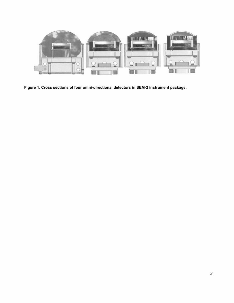
In the SEM-2 package, the two lower energy detectors (P6 and P7) have 2-s integration times while the higher energy detectors (P8 and P9) have 4-s integration times. For this algorithm, the detectors are referred to as numbers 0 (lowest energy) to 3 (highest energy). Cross sections of the four omni-directional detectors in SEM-2 instrument package are shown in Figure 1. It can be seen that the higher energy detectors (on the left) have more shielding on the domes.
Figure 1. Cross sectionns of four ommni-direction
al detectors in SEM-2 insstrument pacckage.
9
10
3 ALGORITHM DESCRIPTION
3.1 Algorithm Overview
The EI algorithm converts ion count rates (ions/sec) into differential flux spectra with units of ions / (cm2 s sr MeV). The basic equation to be solved is to determine the differential proton flux j(E, θ, φ) from the count rate ci for channel i:
, , , , sin ∞
where b is the background count rate, dA is the area of the detector, dt is the duration of the measurement, E is the energy, GB(αB, θ, φ) is the particle angular distribution function for the pitch angle αB, Gi(E) is the detector response including the field of view (FOV), and ηi represents the change in response due to detector aging,
The fundamental assumption of this algorithm is that over short energy ranges the differential directional energy spectrum of solar ions above 1 MeV follows a power law in kinetic energy, with an exponent that varies with energy. This assumption is well supported by observations of solar and magnetospheric ions with energies in the 100’s of keV to MeV range [e.g., Baker et al., 1979; Lario and Decker, 2002].
The four omni-directional detectors provide the EI algorithm with 1-s proton count rates in four overlapping energy bands: 16-35, 35-250, 70-250, and 140-250 MeV. First, the algorithm redistributes the count rates into a new set of four non-overlapping energy channels. Then it iterates a piecewise power law fit over adjacent channels in order to derive a differential flux spectrum. The calculations include the energy-dependent geometric factor (response function + FOV) for each detector channel. The basis of this algorithm is the SEISS Integral Flux Algorithm for GOES-R [Rodriguez, 2009].
The primary algorithm outputs are four pairs of power law exponents and coefficients which define the derived differential flux spectrum over the entire energy range of the input channels. Also produced is the total flux in each of the five non-overlapping channels. The algorithm sets limits and defaults on the value of the power law exponents, , in order to
avoid using unrealistically extreme or noise-sensitive values of this parameter. Since is solved iteratively, the algorithm places a limit on the number of iterations. Flags are set when defaults are used, limits are reached, or input data are missing.
3.2 The Particle Environment Measured by POES
The greatest proton fluxes above 10 MeV are observed during solar energetic particle (SEP) events. These energetic ions (as well as electrons and heavy ions) are believed to originate
11
in shocks and magnetic field reconnections associated with coronal mass ejections (CME) [Cane and Lario, 2006]. The measurement of proton fluxes in polar orbit has both operational and scientific applications. These fluxes are sufficiently energetic to impact satellites in the region, causing undesired transient responses and single-event upsets and permanent damage in solid state and solar cell devices [Baker, 1996]. Measurements of proton fluxes support alerts and warnings of radiation hazards to occupants of manned spacecraft and polar-crossing aircraft [Baker, 1996] and serve as inputs to operational predictions of D-region absorption of high-frequency and very-high-frequency (HF/VHF) radio waves [Sauer and Wilkinson, 2008] and to models to determine the polar cap boundary.
On its polar orbit, POES passes through several different regions of higher proton concentrations. Ions from SEP events are detected at high L-values (above about L>2.5) where they are directly injected into the polar regions during geomagnetic storms. The SEPs have a broad spectrum and are detected in all of the OMNI instruments. Following geomagnetic storms, new proton belts with energies in the 2-15 MeV range are sometimes created from ions injected at locations of about L=2 to 3.5 [Lorentzen, 2002]. A third set of energetic ions encountered by POES are those in the South Atlantic Anomaly (SAA). These trapped ions have energies covering all bands of the omni-directional detectors. In the SAA the ion fluxes are found mostly at L<1.6 and are not impacted by magnetic activity or SEP events [Evans, 2008].
Background counts on POES are due to galactic cosmic rays (GCRs) and are highest near the magnetic poles. The background count rates are below 1 cps. An example of a quiet period from POES data is shown in Figure 2a. An example of the high count rates detected during a SEP event is shown in Figure 2b.
Figure 2. PNOAA-15 ov(1 January temporary pshowing the
The calculsingle statsimplify thewith a powadequately(Figure 3)acceleratio
Proton countver six-hr pe2003) showi
proton radiate high count
ation of thetistical repre calculatio
wer law, j(E)y by a sing, in which
on of the so
ts in the lowriods. Also ing backgrotion belt. (b)rates over th
e differentiresentation n. For exa
) = j0 Eγ. In
gle power lh the highource popu
west channeshown are tund counts
) Data takenhe poles due
al flux requof the sp
ample, a mo general, hlaw. The est energi
ulation to M
l (≥16MeV) ohe L-values due to GCR
n during a lae to SEPs and
uires assumpectrum caonotonic deowever, theonset of aes arrive
MeV energi
of the POESat the satellRs as well aarge geomagd the peaks
mptions aban adequatecrease in e spectrum SEP evenfirst (withi
ies). Durin
S omni-directite. (a) Data as peaks frognetic stormdues to the S
bout its spetely fit theflux with en
m of SEPs isnt is a veryin tens of ng such a
tional detectfrom a quietom the SAA
m (29 OctobeSAA.
ectral shap data,that nergy mighs not represy importan
minutes period, wh
12
tors on t period
A and a er 2003)
pe. If a would
ht be fit sented t case of the en the
data clearsingle eneadequatelinterest, ituses a pie
Figure 3. Rthe onset oafter Bryan
The SEPsdistributiorange (remagnetic below w
∝[Evans, 2form sinn much largoverlap ofalgorithm are mis-co
rly exhibit vergy spectly represent is better ecewise fit o
Rapid evolutof the SEP evnt et al., 1962
s, which on. Trapped
elative to thfield at the
which any
/008]. The [(α / αmax )
ger. The anf the pitch include en
ounted as p
velocity disrum. Therented by a not to basof power la
tion of the 1vent of Septe
2, Figure 11].
ccur at higd ions, whiche B field)satellite, a
particle
/ ; the a
pitch angle90˚] where
nalysis in thangle distrergetic neuprotons.
persion, thefore, since
single poe the calcuw functions
00-600 MeV ember 28, 19
gh L-valuesch are dete) between nd B120 is t
is assum
angles outs
e distributioe n is frequhe EI algoritribution of putral ions, s
e exponente the differ
ower law dulation on s to the spe
spectrum o961, as meas
s, are assuected at low90˚ ∝
the magnetmed to
side of this
on of the traently chosethm does nparticles. Osatellite cha
t varies frential flux distribution,this assum
ectrum.
of solar protosured by Exp
umed to hawer L-values
and 90tic field strebe lost
range are
apped parten to be 2, not currentlyOther errorarging, and
from positivspectra a
especiallymption. Inst
ons at 7-minplorer 12 [ fro
ave an isos, occur in 0˚ ∝ , ength at an to the a
referred to
icles is assbut near th
y include cor sources nhigh energ
ve to negatre sometimy during titead the al
nute intervalsom Rodrigue
otropic pitcha local pitcwhere Bsat
altitude of atmosphere
o as the los
sumed to hhe equator onsiderationot includedgy electrons
13
ive in a mes not mes of gorithm
s during ez, 2009;
h angle ch angle
t is the 120 km
e, and
ss cone
ave the may be n of the d in the s which
14
3.3 Mathematical Description
The EI algorithm determines the differential proton flux spectrum from the proton count rates produced by the SEM-2 omni-directional detectors. Challenges in this algorithm are that there are only four input channels, the channels overlap in energy, and there are energy-dependent correction factors.
The count rates are an integral of the differential flux and geometric factors. In order to estimate the integral of a function, a summing method can be used. The range is segmented into sub-ranges where the area under the curve can be well-represented by a simple function. These pieces of smaller area are then summed to provide the total integral. This estimation becomes better as the sub-ranges are made smaller.
The sub-ranges in these calculations are defined by the bandwidths of the detectors, and therefore cannot be made narrower to more accurately represent the differential flux spectrum. The proton measurements are made in channels that are rather wide in comparison to the energy dependence of the differential flux spectrum. Since the spectrum between the measurement values is not likely to be linear, we improve the estimation by applying an appropriate functional form to the curve between measurements. At these energies, a power law is a physically acceptable model of the differential flux spectrum that has been used extensively in legacy algorithms.
This procedure is based on the approach of the SEISS Integral Flux Algorithm for GOES-R [Rodriguez]. For the POES/MetOp EI algorithm, the particle count rates, Ci, are in adjacent channels with non-overlapping energy ranges. Center energies, Ei, are defined for each channel, i, and then power law fits of the differential flux,
, (1)
are made over the ranges between the center energies. The power law expression implicitly assumes that the energy is normalized to some reference energy such that j0,i is the flux at this energy and the term is a unitless function. For the solar proton integral fluxes, the natural reference energy is 1 MeV and the differential flux units are ions cm-2 s-1 sr-1 MeV-1. Constraints are that the differential flux from adjacent fits must match at the center energies,
,
and that Ei is a midpoint (i.e., "center-of-mass") energy such that
.
15
where the Gi are the detector effective geometrical factors. A solution to these equations is found by iteratively calculating the channel center energy, Ei, and then the power law parameters, j0,i and γi, until the values of Ei converge.
Several modifications to the GOES-R procedure were required for use with the SEM-N data in the EI algorithm. First, the GOES-R technique assumes that the detectors have a constant response as a function of energy. The EI equations can maintain a similar form with the approximation that the detectors have piecewise power law responses. The GOES-R technique also requires that the detector channels should not overlap. For the EI algorithm, this requires converting the given overlapping channels into non-overlapping channels. This is done with some initial fit estimates using default values for the power law exponents.
The proton differential flux spectrum, ji(E), and the detector response, gi(E), are assumed to have power law forms in each region i:
(2)
To simplify the following expressions we define:
(4)
The associated count rate over region i is
, (5)
,
(6)
where Eu and El are the upper and lower limits of energy range i. From Eq 6 we obtain an equation for the differential flux coefficient:
,
(7)
Next we define an "uncalibrated flux", k, which is the detected differential flux without the geometric factors. This is given by
(8)
In region i, there is some midpoint energy Ei (Figure 4) such that
16
, (9)
The initial guess for each Ei is the geometric mean in the energy range given by
(10)
To derive the power law fit, we take the ratio of the ki and ki+1 at Ei noting that ji = ji+1 since the adjacent fits should match at this point.
, ,
, (11)
Given that and log log log , we find
,
,
/
The power law exponent for this region is then
/ ,
⁄ (12)
Given γi (and hence βi), we can now find the new Ei for this iteration. Reordering Eq. 9 and substituting from Eqs 8, we get
,
(13)
Substituting for Ci from Eq 6 yields
(14)
/
(15)
Then, the power law coefficient determined from Eq 9 is
, (16)
17
In practice, the calculations of γi and then Ei and j0i are iterated until the change in Ei is adequately small. The integrated flux can be calculated with the final values of γi,Ei and j0i is
, (17)
, (18)
3.1.1 Simple Fit
As described in the next section, for cases where there the count rate is low, a simple fit to the data is made with a single power law using count rates in the lowest two non-overlapping channels. A "two point" fit is preferred, but if that cannot be made, then a "one point" fit is made. The fit of two channels to a single power law is done as follows at E0 and E1. First, using ax = exp(x log a), Eq. 1 expands to
(19) Here the subscripts have been removed, since there will be only one power law fit for all ranges. A linear expression is created by taking the logarithm of both sides of Eq. 19 to produce ln ln ln (20) For two midpoint energies, E0 and E1 and with an estimate of the flux at each of the energies, the power law parameters of j0 and γ are then
⁄
⁄ and (21)
/ (22)
For a single point fit, for the energy, Ei, the flux parameters are
and (23)
18
/ (24) In this case, the j0 used is the average of that calculated at E0 and E1.
Figure 4. Tand El) andifferential energies.
3.4 Proce
A summais referredgeneratedNo backg(Figure 2)
1. Redirebe
2. Geexp
3. Cothenewcha
4. Initinit
5. Ful
The relative ld the midpo
flux (ji) are
essing Pro
ry of the std to as "rawd non-overlground subt).
ad in raw pectional detset to -999
enerate initiaponent, γdef
nvert raw ce initial diffew count rateannels is <1tialize Ei witial values dll fit routinea. Estima
the hig(Step 6
b. Estima
ocations of soint energiese offset sin
cedure
teps in the w count ratapping chatraction is
proton countectors. If a
9. al estimates
fault. (Eq 7) count rates erential flux es are nega1, skip Stepth the geomdo not impa: Iterate to dte the set ohest energy
6). te a new se
some variabs (Ei). Note
nce the diffe
algorithm ftes" and "raannels are performed
nt rates in ovany of these
s the differe
to count raspectrum. ative, or if tps 4 and 5 ametric meanact the solutdetermine p
of γi using thy leg is pos
et of Ei usin
les includingthat the ran
erential flux
follows. Thaw data chreferred tobecause th
verlapping e values ar
ential flux s
tes in four n If the sum
the sum of tand do the n of the chation. power law phe set of Ei
sitive (|γ2 |>0
ng the new
g several upnges for ch
fits are ca
he original dhannels", wo as just "che backgro
energy chare negative
spectrum us
non-overlapof raw cou
the count rasimple fit ro
annel edge
parameters
i. (Eq 12) If0), then ski
set of γi. (E
per and lowehannel countalculated be
data in ovewhile that incount ratesound count
annels fromor NAN, th
sing a defa
pping energunt rates < 2ates in the outine in Stenergies. (
s, j0,i and γi.f any |γi |>8ip to the sim
Eq 15)
er channel et rates (Ci), tween the m
erlapping chn the EI-algs" and "chat rates are
m the four ohen all outp
ult power la
gy channel25, if any ofthe first thrtep 6. (Eq 10) Th
. 8 or if the smple fit rout
19
dges (Eu and the
midpoint
hannels gorithm-annels". <1 cps
mni-ut will
aw
s using f the ree
ese
slope in tine
20
c. Since there are two Ei’s associated with each channel (except for the lowest and highest energy channels), one below the center energy and one above the center energy, there are two new Ei’s for each channel. Linearly average the two estimates to derive the new estimate of Ei going forward.
d. Compare new Ei with previous Ei. Reiterate Steps 5a-d until the convergence criterion that all channels are changing by < 1% is met. If, after ten iterations, the value of Ei is still changing by more than 1%, then stop the iteration and do the simple fit routine in Step 6.
e. Calculate the set of j0,I from the final set of Ei and γi. (Eq. 16) f. Extrapolate from the adjacent fits to cover both ends of the range of the
channels; i.e., select γ0 and j0,0 for El,0 to E0, and γ4 and j0,4 for E4 to Eu,4. 6. Simple Fit Routine: If there were errors in converting from raw count rates or during
the iteration, generate a single power law fit to the entire differential flux spectrum using the count rates for channels 0 and 1. For either type of simple fit (one-point or two-point) the resulting γ< 0. Before starting the calculations, if cn[ii]<0 for ii=0 or 1, that cn[ii] is set to 0.
a. Estimate j(E0) and j(E1) for the lowest two channels. (Eqs 8 and 9) b. If C0>0.01, C1>0.01, and j(E0)>2* j(E1), and then do a
Two-point fit: use j(E0) and j(E1) to define a single power law fit over all channels (Eqs 21 and 22).
c. If didn't do a two-point fit or the two-point fit produced γ< -8, then do a One-point fit: If either j(E0) or j(E1) is <0.00001 it is reset to 0.0001 Determine the coeficients, γ0 and γ1, at both E0 and E1 using Eq. 24. The final parameters for the single power law fit over all channels are the default power law exponent, γdefault, and the average of j0(E0) and j0(E1).
7. Calculate differential flux at desired energies to output. (Eq. 1) 8. Calculate estimated errors on differential flux (Section 4.5). 9. Set exception handling flags as needed.
In general, the non-simple fit requires only two or three iterations to converge. Setting the convergence threshold to 0.1% or less has a negligible effect on the results and increases the number of iterations by at most one.
A default power law exponent, γdefault, is used at several points in the algorithm. The value of -2.9 was obtained by temporarily setting all of the fits to simple fits and finding the average γ for 2-pt fits of NOAA-15 data for the year of 2003.
Differentiaestimateswhich dete
The convein non-oveportrayed done in ppiecewisechannels
The next range 140and γdefaul
j3 and the an estima
The countthe geomneeded to
MeV. Fromchannel is
Figure 5. Tand the derand geome
al flux is cal are given ermines γi a
ersion fromerlapping cin Figure
piecewise fe in energy.cover the s
step is to 0 to 250 M
t. Next, threlevant ge
ate of j2 is m
t rates on thmetric factoo calculate m C1 an es given by C
The overlapprived non-ov
etric factors.
lculated in tover the chand j0,i is ap
m the raw cohannels, C5. The sufashion be. Calculatiosame range
determine MeV is mad
he count raeometric fa
made.
he lower thr ranges dthe count r
estimate of C0 = O0 – C
ping energy rverlapping ra
two ways ahannel rangpplied to th
ount rates o
i, requires subtraction oecause the ons are sta
e from 140 t
C2. First ae using Eq
ate in this ractor for cha
hree energydo not oveate there: Cj1 is made
C0,j2,90-140 MeV
ranges of theanges for the
and over twges using Ee ranges be
of the omniseveral stepof count rat
functions arted from tto 250 MeV
an estimateq. 7, the reange on deannel 2, g2.
y channels aerlap perfecC1 = O1 – Ce. Similarly
V - C0,j2, 70-9
e raw count re final count
wo different Eq. 6 and γd
etween the
i-directionaps. The eletes from thfor the ge
the highestV, C3= O3.
e of differeelevant geoetector 2, C
Then C2=
are found ictly for ch
C1,j3,140-250 M
, the coun
90 MeV– C0,j1
rates from thrates, Ci. A
sets of regi
default. The e midpoint e
l detectors,ements of the various eometric fat energy ch
ential flux fuometric factC2,j3,140-250 Me
O2 – c2,j3,14
n a similar annel 1, m
MeV – C1,j2,90
t rate for t
, 35-70 MeV.
he omni-direcAlso shown a
ions. Rougiterative fit
energies.
, Oi, to couhis converschannels m
actors are hannel. Sin
unction j3 otors for cha
eV, are foun
40-250 MeV. F
fashion. Bmultiple ter
-140 MeV - Cthe lowest
ctional detecare the non-z
21
gh initial routine
nt rates sion are must be defined ce both
over the annel 3, nd using From C2
Because rms are C1,j2, 70-90
energy
ctors, Oi, zero FOV
The simplesmall. Thbackgroundthe calculacount, andwhen the (generally backgrounddetector coenergy chaentire rang
A cartoon oshown as discontinui
Figure 6. Cextrapolated(black line).
3.5 Algorit
The input tdetectors, a
3.5.1 Prim
The differesampling t
e fit routine his occurs d levels. D
ation of γi a not represpower law lower enerd levels. Tount rates iannels and e.
of the technwell as
ties occur a
Cartoon of td to edge of The count r
thm Input a
to the algorand ancilla
ary Senso
ential flux catimes are 2
is used whwhen the uring theseand j0 can sentative offits produc
rgy ones) hThe threshois <25. Fouses just t
nique is shothe extrapat the Ei.
echnique. f energy rangrates, Ci, for
and Outpu
rithm consiry data des
r Data
alculation u2 s for the
hen some oparticle flu
e times whebe greatly
f the actuace very larghave very hld for using
or the simphe first two
ow in Figurpolations to
Power lawsge (dashed
r the four det
ut
sts of the cscribing the
uses the foue two lowe
of the convuxes in somen the mea
y affected bal populatioge exponehigh countg the simplele fit routin
o channels t
re 6. The to the edg
s are calculpurple lines
tectors are re
count ratesresponse f
ur channelser energy d
verted counme of the asurementsby small van. The simnts; this ocrates, but
e fit routine ne, the algoto set a sin
three poweges of the
ated betwees). The true epresented b
s from the ffunctions of
s of the OMdetectors a
nt rates areenergy ch
s may be inariations inmple fit rouccurs whenadjacent ch is when th
orithm disrengle power
r law fits bee detector
en Ei (solid differential
by the blue b
four SEM-2f the individ
MNI proton and 4 s fo
e negative ohannels aren the noise
n the backgutine is alson some chahannels are
he sum of thegards the law fit acro
etween theranges.
purple lineflux is also
boxes.
2 omni-diredual detecto
count ratesor the two
22
or very e near e level, ground o used annels e near he four higher
oss the
Ei are Slope
es) and shown
ctional ors.
s. The higher
23
detectors. The accumulation times end 0.2 s after time stamps according to Evans and Greer [2000].
In specifying the FOV center direction relative to the ENP coordinate system, it is assumed that the spacecraft axes are aligned to this coordinate system (where N is the normal to the orbital plane and E is directed toward the Earth along this plane). Given the large FOVs, this is not a critical assumption for small (~1 deg) differences between the spacecraft and ENP axes. The omni-directional detectors are mounted on the spacecraft with the central axis of the dome directed off-axis to E and along P by 9˚ [Evans and Greer, 2000].
Table 2. SEM-2 OMNI 1-s inputs to EI algorithm.
Quantity Number of Values Units Purpose in Calculations
Proton count rates 4 cps Basis for flux calculations
3.5.2 Auxiliary Data
No auxiliary data is needed by the algorithm.
3.5.3 Ancillary Data
Ancillary data are data that are not generated by SEM-2 or the spacecraft on-orbit or by the ground processing system. The ancillary data required by the EI algorithm include of characteristics of the OMNI channels (Table 3). These characteristics consist of their response functions (i.e., geometrical factors) as a function of energy. These data are products of the characterization of the HES in ground test and analysis. The geometrical factors are fit with power laws as a function of energy for ease of use in the EI algorithm. For some detectors, with a flat response at low energy, there are power laws fits for two energy ranges.
Table 3. Ancillary data related to OMNI performance characteristics required by the EI algorithm.
Quantity Refresh Number of Values Units Purpose in
Calculations Source
Energy boundaries of detector response function
Static
3 energy boundaries (representing 2 energy ranges)
MeV
To calculate band centers and average fluxes
Ground calibration
24
Quantity Refresh Number of Values Units Purpose in
Calculations Source
Detector response functions
Static
Power law response functions (1 exponents and 1 coefficients) on one or two energy ranges for each of the detector. In software version 1.0 there are a total of 6 functions for the four detectors.
cm2 sr To calculate average fluxes
Ground calibration
Software version number
Static
Two integers (i, j). Version number is of the form "i.j"
none
May define changes to other static values.
Software
Output energy values
Static For software Version 1.0, there are 3 energies: 25, 50 and 100 MeV.
none
Energies at which to calculate output average fluxes
Software
3.5.4 Algorithm Output
The EI algorithm creates power law fits to the differential proton flux spectrum. The fits are made to three adjacent energy intervals which fully cover the energy range of the four input channels. The coefficients, exponents and energy ranges of the fits are output. Other output values include the differential flux at three specific energies chosen to be near the geometric means of the channel energies, the fractional error on the flux and quality flags. The data outputs are shown in Table 4 and flag outputs are shown in Table 5. The non-integer output values are converted to float data types from doubles to save file space.
Table 4. Data output from EI Algorithm.
Name Description Data Type Number of
values Units
Eedge1 Boundaries of energy ranges for power law fits to differential proton flux
float 4 MeV
25
Table 5. Flags output by EI algorithm. All flags are integers. Values are 1=true, 0=false unless otherwise stated.
Flag Cause Result
bad_cn Non-overlapping channel count rates are 'NaN'. Note: this seldom if ever occurs.
Record is not processed.
bad_omni_cts OMNI count rates are negative or 'NaN'. Record is not processed.
fit
-1= No fit performed.
0= Power law fit with different γ and j0 over four regions
1 = simple "one point" fit: Fit all energies with a single γ and j0 based on count rates in first two channels and γ= γdefault.
2 = simple "two point" fit: Fit all energies with a single γ and j0 based on count rates in first two channels.
Defines fit used.
gamma_lim For some i, | γi | >8. Use a fit with a single γ and j0.
highE_slope_pos Initial fit produced slope>0 (γ2 >0) for highest energy range
Use a fit with a single γ and j0.
jf0 Coefficients of power law fits to differential proton flux
float 3 ions / (cm2 s sr MeV)
gamma0 Exponents of power law fits to differential proton flux
float 3 none
j_out Differential proton fluxes at 25, 50 and 100 MeV
float 3 ions / (cm2 s sr MeV)
fract_err Average fractional error on fluxes
float 1 none
[flags] Error/quality flags (see Table 5) int 6 see Table 5
version EI software version number int 2 none
26
Flag Cause Result
iter_lim For some i,, exceeded number of allowed iterations (10) to determine Ei.
Use a fit with a single γ and j0.
27
4 TEST DATASETS AND ERROR BUDGET
The proxy data for the OMNI detectors is discussed in Sections 4.1 through 4.3. The sources of error for this algorithm and the error calculations are discussed in Section 4.4.
4.1 Simulated/Proxy Input Data Sets
The proton differential flux calculation requires input of proton count rates in four channels. Proxy count data are created from several sources and are intended to represent a wide range of conditions for the OMNI detectors. The test data sets include a mix of quiet and active times and include occurrences of solar energetic particle (SEP) events. Proxy data include some extreme values and bad data points that can be used to exercise the algorithm. The software was set up to generate proxy data with either a prescribed spectral function or from POES 16-s averaged data.
To evaluate the errors due to the algorithm, the proxy data count rates must be generated from a "true" spectrum, and then the output of the algorithm compared with this "truth". This type of proxy data is created by (1) generating "true" differential energy spectra from real count data, and then (2) generating proxy SEM-N count rates based on these "true" spectra. The first step requires assumptions regarding spectral shape. The chosen spectral shape does not need to match reality perfectly in order for the generated spectra and associated proxy count rates to be good tests of the algorithm. Poisson noise can be added to the count rates to assess its impact on the algorithm as discussed in Sections 4.4 and 4.5.
4.2 Proxy data from POES measurements
Simulation software was set up to generate proxy data over any time range from 16-s averaged POES or MetOp OMNI data. The data was accessed from the NOAA NGDC archives and generally the NOAA-15 data was used to create the proxy values. The lowest channel of the POES omni-directional detectors is known to be contaminated by electrons, but this is not considered in the creation of the proxy data.
The EI algorithm is run using the proxy POES raw count rates and differential flux spectra are generated for the entire energy range of the detectors. These spectra are not used as "truth" because they have unrealistic discontinuities in slope at the center energies. Instead, the "true" spectrum is created by fitting the differential flux values, ji at each of the center energies, Ei with a pair of overlapping power law functions. The lower energy fit is over j0, j1, and j2, and the higher energy fit is over j1, j2, and j3. The fit is accomplished by doing a linear fit to ln j. The final spectrum is an interpolation of the two fits in the overlapping region between E1 and E2. Then, proxy detector count rates due to the "true" spectra are calculated assuming response functions of the OMNI detectors. The proxy
28
count rates are run through the algorithm and the differential energy flux spectrum output by the algorithm is compared to the "true" spectrum.
Table 6. POES omni-directional data channels.
algorithm channel number
POES channel POES channel energy
range (MeV)
0 P6 16-250
1 P7 35-250
2 P8 70-250
3 P9 140-250
Proxy data sets using POES data can be chosen to encompass SEP events including their onset, peak, and decay, and the magnetospheric-only populations preceding or following them such as the events that occurred over 10 days during the 2003 Halloween storm.
4.3 Proxy data from 2003 SEP fluence spectra studied by Mewaldt
The algorithm was also tested on data for the SEP events of October-November, 2003. Mewaldt et al. generated fluence spectra for five events during this time period using double power law fits:
⁄ exp ⁄ for ;
⁄ for
The spectral functions defined by Mewaldt et al. were used to generate proxy count rates which were then processed by the EI algorithm. A comparison of the original spectra and the EI algorithm output are shown in Figure 7. For all points shown for the five cases, the average magnitude of the error was 2.4% with a standard deviation of 4%. There is no noise on this data, so it is a test of how well the algorithm fits the fluence spectral shape.
Comparison 2003 given from the eqoduced by thl spectra is 5
r Determina
e a numbeFactors in
esolution, oa, and algo
algorithm plunt rates fothm with pro
of power lawin Table 5
uations fromhe EI algorit5%.
ation
er of sourcnclude unceoverlap of rithm error.
us instrumeor each chaoxy data to
w fits to proof paper by
m Mewaldt etthm. The a
ces of erroertainties indownward
.
ent error isannel are c
o obtain the
ton fluence y Mewaldt (t al., and theaverage stan
r that contn instrume
loss cone
determinecalculated. statistics o
spectra for f2005). Thee solid linesndard deviati
tribute to unt correctio
e with dete
ed in two st Then, this
on how it im
five SEP evee dots are t
s are the powion for the d
uncertaintieon factors,
ectors, Pois
eps. First,s error is pr
mpacts the o
ents during Othe spectralwer law fits derived spec
es in the Elow spect
sson noise
the error bropagated toutput fluxe
29
October- shapes to those
ctra from
EI EDR tral and
on the
budgets through
es.
Figure 8. Er
Figure 8 shchannel. H
given by
z
4.5 Error E
As discussrates and tshown in F
rror propaga
hows the erHere, the ro
z
z
x
x
2
Estimates
sed in Sectthen proxy Figure 9.
tion for the c
rror propagoot sum of
y
y
2
.
tion 4.1, focount rates
count rates i
ation of thef the square
r tests, "trus are gener
n one chann
e main soures of indep
ue" spectrarated from t
nel.
rces of erropendent rel
a are generthese "true"
ors for the cative unce
rated from " spectra.
count rates rtainties (R
(25)
the POESAn examp
30
in one RSS) is
count le fit is
Figure 9. with diamo
To determoutput spein a little mMeV, andfunction ochannels course, duused thes
Based on
Σo
where omAbove thi0.27, andConsidericonservat
Table 8 sthe algoritthe valuesattempt toalgorithm error in th
Comparisononds.
mine the errectra were more detaild >100 MeVof the counto see how
ue to Poissse results to
the values
omni[i] >25
mni[i] are ths threshold
d 0.38 and ng that wtive estimat
hows the frthm. Whers come froo calculate
(final coluhe knowled
n of typical fi
ror statisticscompared , by breakinV. We loont rates in w the standon noise, w
o set the thr
in Table 7,
e count ratd are avera
an overallwe are onlyte of the err
ractional erre the error
om the marerrors, butmn of Tab
dge of the e
t of flux (dot
s, Poisson with the "trng up the oked at the both the lo
dard deviatwe expect tresholds for
, we choose
tes of detecage standal average sy looking rors.
rror as a fur is based rked valuest rather set le 8) includeffective ge
tted line) to t
noise was ue" spectra
output into tstandard d
owest enertions changhe largest dr when the
e a thresho
ctor channerd deviatiostandard dat certain
nction of thon the sums in Table this error t
des an addeometric fa
the "true" flu
added to ta. We examthree energdeviations irgy channeged with lodeviations asimple fit s
old for the fi
el i and Σoons in the tdeviation of
spectral
he detector m of the de
7. For theto 1.0 (100ditional erroactor (Sectio
ux (solid line
he proxy comined the stgy bands: 1in each of el and the ow and highat the lowe
should be a
it routine of
omni[i] is ovthree energf 0.36 (lastshapes, th
count rateetector coune simple fit
0%). The eor due to aon 6.1) wh
e). Errors ar
ount rates tandard dev6-50 MeV, these bandsum of al
h count ratst count ratpplied.
f
ver all 4 chgy ranges ot line of Tahis is prob
es that is ount rates (Σot case, we error outputan estimatehich is adde
31
re shown
and the viations 50-100
ds as a l of the tes. Of tes. We
hannels. of 0.36, able 7). bably a
utput by omni[i]),
do not t by the ed 20% ed as a
32
root sum of the squares (Eq 25). This is a conservative estimate of the error. Other unquantified sources of error include the assumed spectral shape that we used for the proxy data and the assumption that the particle angular distribution is isotropic.
Table 7. Standard deviations (fractional error) of flux for three energy bands for the NOAA 15 satellite. Other thresholds were set to minimal values. Here Σomni= omni[0]+omni[1]+omni[2]+omni[3], where the omni[] are the original channel count rates.
Table 8. Error values output by the EI algorithm.
simple
fit range for Σomni
fractional error based on
Poisson error only (from
Table 7)
fractional error output by
algorithm (includes 20% error
on detector response)
no 25<Σomni<50 0.74 0.77
50<Σomni<100 0.62 0.65
'' 100<Σomni<250 0.45 0.49
'' 250<Σomni<500 0.34 0.39
'' 500< Σ omni<1000 0.29 0.35
date(s) threshold
avg sd
for j in 16‐
50 MeV
avg sd
for j in 50‐
100 MeV
avg sd
for j in
>100 MeV
avg sd
for j over
full range
no. of
values
in avg
used to
define
output error
2003‐
05 15<Σomni<25 2.77 0.44 0.52 1.17 3800
2003‐
05 25<Σomni<35 1.52 0.41 0.54 0.75 4100
2003 25<Σomni<100 1.28 0.40 0.51 0.67 9500
'' 25<Σomni<50 1.44 0.42 0.56 0.74 3300 x
'' 50<Σomni<100 1.19 0.39 0.48 0.62 6000 x
'' 100<Σomni<250 0.75 0.33 0.38 0.45 11000 x
'' 250<Σomni<500 0.51 0.26 0.31 0.34 10000 x
'' 500< Σ omni<1000 0.42 0.22 0.27 0.29 12000 x
'' 1000<Σ omni<5000 0.46 0.19 0.12 0.22 33000
'' Σ omni>5000 0.38 0.24 0.22 0.25 2000
'' Σ omni>1000 0.46 0.19 0.12 0.22 35000 x
'' Σ omni>25 0.66 0.26 0.29 0.37 78000
Oct
2003 Σ omni>25 0.50 0.26 0.36 0.37 11400
2000‐
09 Σ omni>25 0.72 0.26 0.28 0.37 850000
33
'' Σ omni>1000 0.22 0.29
yes any, but generally Σomni<25 1.0 1.02
For proxy data created from the POES data, output statistics are shown in Table 9. The values were determined with a threshold for non-simple fits set to Σomni[i] >25 and Poisson noise added to the detector count rates.
Table 9. Statistics and other values for output spectra with added Poisson noise.
4.6 Other Tests
A simple test was performed to compare the outputs of this algorithm with the simple directional flux estimates given as J6-J9 in Appendix F of Evans and Greer (2006) for the POES OMNI detectors. These fluxes are calculated for energy ranges 16-35, 35-70, 70-140, and 140-500 MeV. Directional fluxes were calculated for the same ranges from the fits given by this algorithm (Table 10). This comparison verifies that the magnitudes of the algorithm output are reasonable. It also shows that some refinement is needed for the very simple Evans and Greer (2006) algorithm because it sometimes produces negative fluxes.
year(s) key values for proxy fractions of data statistics
Table 10. Six examples of comparisons of fluxes output by algorithm with fluxes from simple calculations of Evans and Greer (2006).
trial # channel count rate Evans flux flux from algorithm fit
1 0 29 3 11
1 25 ‐8 4
2 34 3 13
3 16 3 10
2 0 213 15 23
1 195 27 64
2 163 6 67
3 130 24 82
3 0 1576 841 892
1 586 199 336
2 352 49 161
3 81 15 46
4 0 3134 1483 1187
1 1387 347 716
2 978 160 403
3 99 18 53
5 0 13039 8729 9708
1 2757 1330 1895
2 1190 205 493
3 66 12 34
6 0 15856 11332 13130
1 2508 1357 1832
2 910 157 382
3 47 9 24
35
5 PRACTICAL CONSIDERATIONS
5.1 Numerical Computation Considerations
The algorithm is straightforward to implement in software. The retrievals do not require matrix inversions. The most complex part of the algorithm, the iterative solution for the channel center energies and gammas, is limited in the number of iterations that can take place and generally requires less than three iterations. Although the measurements are single precision, the calculations takes advantage of the double precision capabilities of the host machine.
5.2 Programming and Procedural Considerations
The operational algorithm has been implemented in C. It uses many subroutines in order to maintain the readability and modularity of the code. The algorithm was originally developed for the proposed NPOESS SEM-N HES instrument and the software retains some variables to permit the 5-channel structure of the HES.
5.3 Quality Assessment and Diagnostics
Quality assessment of the operational product is based on the flags described in the next section. If error flags are set frequently, then either the instrument is having problems or there is a problem upstream in the data processing system. The single power law fits will be used frequently outside of SEP events. The gamma limits should be invoked less frequently, primarily in temporary radiation belts. Based on testing with the proxy data, the energy iteration limit should be reached very infrequently.
5.4 Exception Handling
Instrument error handling is performed prior to this algorithm. Instrument errors or bad data are flagged by setting the detector count rates to -999. This algorithm requires a complete set (4 channels) of count rates to accurately determine the differential flux spectrum. Checks on the validity of the input, based on bad data flags threshold levels for the input are made by this algorithm. The flags are listed in Table 5.
In the presence of one or more missing differential flux values (assumed to be indicated by fill value such as -999.0 or NaN), the algorithm will not calculate the integral flux. Instead, it sets flag_fit to -1, most output values to -999, and any relevant flags to 1. In principle, it is possible to interpolate or extrapolate over a missing flux value. However, there are many possible permutations of missing flux values, and each could require a different algorithm. If the problem is random and infrequent, then it is not worthwhile to develop an algorithm to handle the problem. Should one or more channels in the OMNI fail for a particular satellite, then it may be possible to develop an algorithm to handle the specific situation.
36
5.5 Algorithm Validation
Differential flux measurements could also be compared with those made by the GOES-R instruments as POES or MetOp satellites pass by at much lower altitude. In this case, the differential flux from regions with the same L-value should be compared and the GOES data will need to be converted from integral flux to differential flux.
5.6 Performance
An important performance parameter is continuity of integral flux levels between satellites. Satellite-satellite intercomparisons are needed to ensure continuity of the operational product. Such intercomparisons could be made regarding count rates between various POES and MetOp satellites.
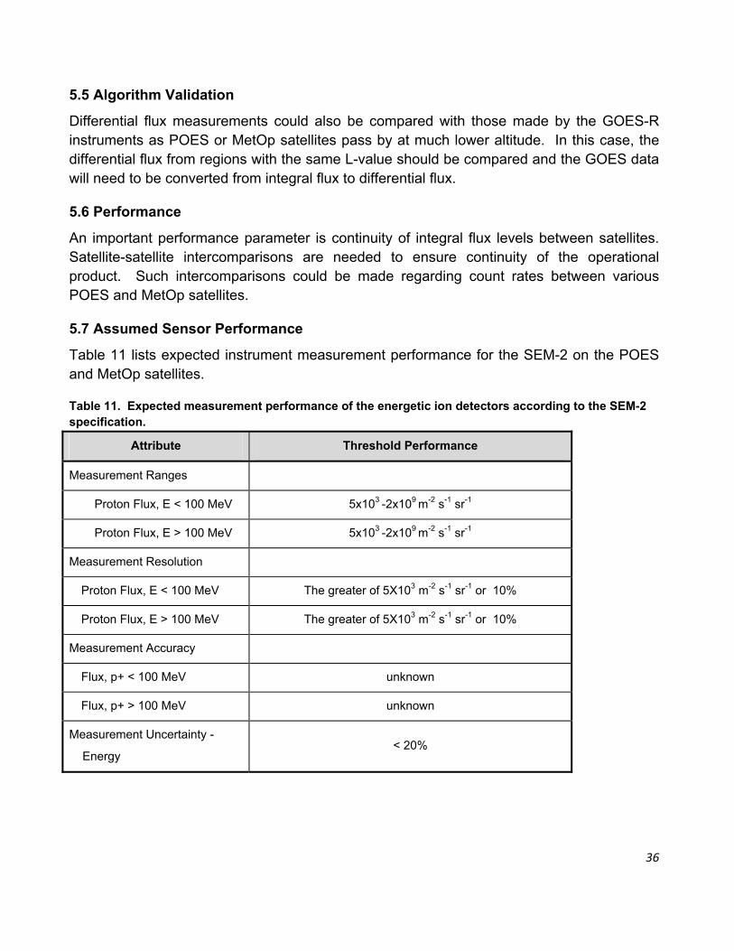
5.7 Assumed Sensor Performance
Table 11 lists expected instrument measurement performance for the SEM-2 on the POES and MetOp satellites.
Table 11. Expected measurement performance of the energetic ion detectors according to the SEM-2 specification.
Proton Flux, E < 100 MeV The greater of 5X10³ m-2 s-1 sr-1 or 10%
Proton Flux, E > 100 MeV The greater of 5X10³ m-2 s-1 sr-1 or 10%
Measurement Accuracy
Flux, p+ < 100 MeV unknown
Flux, p+ > 100 MeV unknown
Measurement Uncertainty -
Energy < 20%
37
5.8 Possible Product Improvements
The lowest energy detector is contaminated by high energy electrons. Tom Sotirelis of JHU-APL is working on an algorithm to remove this contamination.
At low L-values, where the detected ions are primarily from radiation belts, the pitch angle particle distribution should also be included in the analysis. For low pitch angles, the convolution of the pitch angle distribution function could also be included in the calculations given the magnetic field vectors needed to determine the loss cone angle and B-field pointing relative to the detectors. This overlap might be done with the use of a lookup table.
38
6 DETECTOR PARAMETERS
6.1 Detector effective geometric factors
The fields of view for each detector depend on the energy range as discussed by Evans and Greer (2006). The total response for each detector including FOVs was determined by GEANT4 modeling by ATC (Tom Sotirelis, JHU-APL, private communication, 7 February 2012). The GEANT4 modeling was for the three higher energy (35, 70 and 140 MeV) detectors and over a 0.5 cm2 detector area. The aperture was assumed to be 180˚ for the two higher energy detectors and 120˚ for the 35-MeV detector. The particles were assumed to come isotropically from 180˚. The form of the effective geometric factors for one detector is a plateau at low energy (where the height represents the FOV and a detector efficiency of nearly 1) and a fall off at higher energies. For this algorithm, the effective geometric factors were roughly fit to power law functions using the GEANT4 data. The error in these fits was about 20%. For the lowest energy detector (16 MeV), we assumed that plateau height was the same as for detector 1 (35 MeV). The power law exponent for detector 0 was taken to be the average of the exponents for the other three detectors. These values may be updated in future software versions.
Table 12. Power law fits of the form g0i Eδ for the effective geometric factors for detectors obtained
The code is written in C. The main program is omni_flux.c. There are two versions of the wrapping program. For test purposes, one should use omni_flux0 .c while for operational purposes, one should follow the example of omni_flux_calc .c. The primary components of the code package are: makeo make file for omni_flux0.c omni_flux0 .c calls omni_flux and contains needed #defines etc. omni_flux_calc .c same as omni_flux0.c but without test routines omni_flux.h defines output structure omni_testdata.txt test data for omni_flux0.c omni_out_master.txt file should match omni_out.txt when omni_flux0 is run with ITEST=1 In omni_flux.c, the primary flags are isimple 0: do a regular fit; 1: do a simple fit iskip 0: proceed with fit; 1: set all parameters to -999 The primary flow of omni_flux.c is as follows init() initialize variables init_flags() initialize variables set iskip or isimple to 1 based on omni[] if iskip=0 mk_cn() create not overlapping count rates in cn[] set iskip or isimple to 1 if problems if iskip=0 and isimple=0 pl_fit() do piecewise power law fit to data set isimple=1 if problems with fit if iskip=0 and isimple=1 mk_simple() do simple fit with one power law fit to data mk_output() copy output into output structure if iskip=1, flag_fit=-1 and output set to -999
40
7.2 Test data
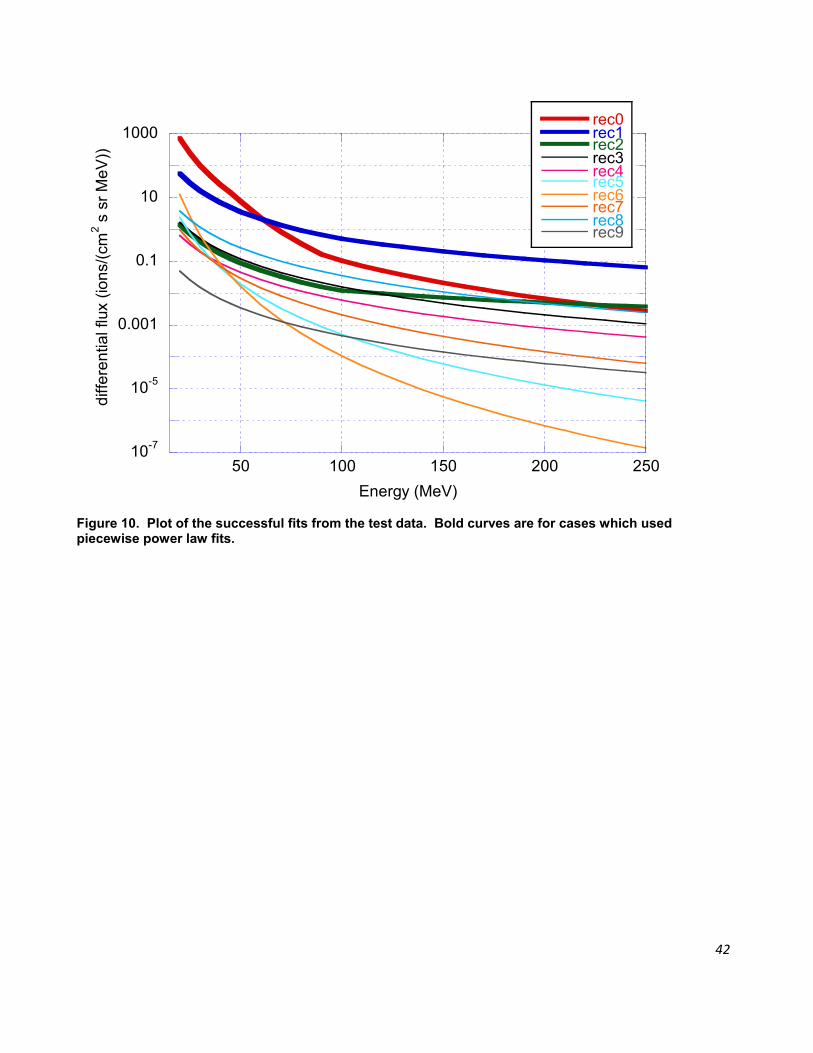
The test data is in omni_testdata.txt. To run the test data, set ITEST=1 in omni_flux0.c. The program will produce an output file omni_out.txt which should be identical with omni_out_master.txt. As of 27 March 2012, the test data file contained: 11 number_of_recs 10000.0 500.0 20.0 2.0 1000.0 200.0 80.0 24.0 25.0 5.0 2.0 1.0 12.0 10.0 1.0 0.0 5.0 8.8 8.0 7.0 -6.0 1.0 2.0 3.0 23.0 2.0 2.0 0.0 80.0 2.0 2.0 2.0 16.0 6.0 8.0 0.0 16.0 26.0 8.0 0.0 1.0 0.0 0.0 1.0 The corresponding output file contained: rec: 0 omni: 10000, 500, 20, 2 err: 0.29 fit type: 0 flags: 0 0 0 0 0 version: 1.0 Eedge1: 16 46 91 250 jout: 248.453 7.656 0.084 gamma: -4.8 -6.5 -3.9 jf0: 1.41504e+09 8.96382e+11 8.10052e+06 rec: 1 omni: 1000, 200, 80, 24 err: 0.29 fit type: 0 flags: 0 0 0 0 0 version: 1.0 Eedge1: 16 49 96 250 jout: 29.218 3.609 0.503 gamma: -3.0 -2.8 -2.3 jf0: 494406 243295 17085 rec: 2 omni: 25, 5, 2, 1 err: 0.77 fit type: 0 flags: 0 0 0 0 0 version: 1.0 Eedge1: 16 49 96 250 jout: 0.732 0.089 0.012 gamma: -3.0 -2.9 -1.3 jf0: 13154.2 8850.24 4.26095 rec: 3 omni: 12, 10, 1, 0 err: 1.02 fit type: 1 flags: 0 0 0 0 0 version: 1.0 Eedge1: 16 49 99 250 jout: 0.885 0.119 0.016 gamma: -2.9 -2.9 -2.9 jf0: 10021 10021 10021 rec: 4 omni: 5, 9, 8, 7 err: 1.02 fit type: 1 flags: 0 0 0 0 0 version: 1.0 Eedge1: 16 49 99 250 jout: 0.339 0.045 0.006 gamma: -2.9 -2.9 -2.9 jf0: 3833.84 3833.84 3833.84 rec: 5 omni: -6, 1, 2, 3 err: -999.00 fit type:-1 flags: 0 1 0 0 0 version: 1.0 Eedge1: -999 -999 -999 -999 jout: -999.000 -999.000 -999.000 gamma: -999.0 -999.0 -999.0 jf0: -999 -999 -999
Figure 10. Plot of the successful fits from the test data. Bold curves are for cases which used piecewise power law fits.
10-7
10-5
0.001
0.1
10
1000
50 100 150 200 250
rec0rec1rec2rec3rec4rec5rec6rec7rec8rec9
diff
ere
ntia
l flu
x (io
ns/
(cm
2 s
sr
Me
V))
Energy (MeV)
43
References
Baker, D. N. (1996), Solar wind-magnetosphere drivers of space weather, J. Atmos. Terr. Phys., 58, 1509-1526.
Baker, D. N., R. D. Belian, P. R. Higbie, and E. W. Hones, Jr. (1979), High-energy magnetospheric protons and their dependence on geomagnetic and interplanetary conditions, J. Geophys. Res., 84, 7138-7154.
Bryant, D. A., T. L. Cline, U. D. Desai, and F. B. McDonald (1962), Explorer 12 observations of solar cosmic rays and energetic storm particles after the solar flare of September 28, 1961, J. Geophys. Res., 67, 4983-5000.
Cane, H. V., and D. Lario (2006), An introduction to CMEs and energetic particles, Space Sci. Rev., 123, 45-56.
Evans, D., H. Garrett, I. Jun, R. Evans and J. Chow (2008), Long-term observations of the trapped high-energy proton population (L<4) by the NOAA Polar Orbiting Environmental Satellites (POES), Advances in Space Research, 41, pp. 1261-1268.
Evans, D. S. and M.S. Greer (2006), Polar Orbiting Environmental Satellite Space Environment Monitor – 2: Instrument Descriptions and Archive Data Documentation, available from NGDC. (http://ngdc.noaa.gov/stp/satellite/poes/documentation.html).
Rodriguez, J., L. Mayer, T. Onsager, J. Gannon (2009), SEISS Integral Flux Algorithm Theoretical Basis Document, version 1.0.
Lario, D., and R. B. Decker, The energetic storm particle event of October 20, 1989, Geophys. Res. Lett,. 29, 10.1029/2001GL014017, 1002.
Lorentzen, K. R., J. E. Mazur, M. D. Looper, J. F. Fennell, and J. B. Blake (2002), Multisatellite observations of MeV ion injections during storms, J. Geophys. Res., 107(A9), 1231, doi:10.1029/2001JA000276.
Mewaldt, R. A., C. M. S. Cohen, A. W. Labrador, R. A. Leske, G. M. Mason, M. I. Desai, M. D. Looper, J. E. Mazur, R. S. Selesnick, and D. K. Haggerty (2005), Proton, helium, and electron spectra during the large solar particle events of October–November 2003, J. Geophys. Res., 110, A09S18, doi:10.1029/2005JA011038.
Sauer, H. H., and D. C. Wilkinson (2008), Global mapping of ionospheric HF/VHF radio wave absorption due to solar energetic protons, Space Weather, 6, 10.1029/2008SW000399.