1

Population growth and the Environmental

Kuznets Curve

Yu Benjamin Fu1, Sophie Xuefei Wang

2, Zhe George Zhang

3

This version: 2014 October

Abstract: the Environmental Kuznets Curve (EKC) hypothesis postulates an inverted U-shaped

relationship between economic growth and many local environmental health indicators, while

some economists argue that the relationship follows other patterns. By using an overlapping

generations (OLG) model, we focus on technological effects, where the properties of the existing

pollution abatement technologies could generate the inverted U-shaped EKC and other forms of

growth-pollution paths for the less developed economies. Moreover, we examine the effects of

population growth on the shape of the EKC, provided that it exists. Simulations indicate positive

population growth raises the height of the EKC at every level of output per worker; thus, putting

extra burden on environment quality. Empirical evidence from China partially supports the

results.

Keywords: Environmental Kuznets curve; Population growth; Technological effect; China

JEL classification: O33, O44, Q56

1. Introduction

The side effects of economic growth on environmental quality have been brought to the

attention of economists since worldwide environmental degradation was observed in the 1960s.

The pessimists believe that growing economic activities will bring even more harm to the

environment, while optimists argue that levels of environmental quality will be improved as

economic development induces cleaner technologies and service-based economy (Meadows et

al., 1972; Syrquin, 1989). Yet a more interesting claim is that the level of environmental

degradation and economic growth measured by income per capita follows an inverted-U shape

relationship (Grossman and Krueger, 1991). This is summarized as the Environmental Kuznets

Curve (EKC): as income per capita increases, measured levels of environmental quality, such as

pollution emissions, also increase at first, but then, after some turning point, start decreasing. If

the EKC hypothesis is correct, it has important implications for sustainable development. First,

1 Postdoc, Beedie School of Business, Simon Fraser University. yuf@sfu.ca

2 Corresponding Author. Assistant Professor, China Center for Human Capital and Labor Market

Research, Central University of Finance and Economics. sophiewang2004@gmail.com 3 Professor, Beedie School of Business, Simon Fraser University. Professor, Department of Decision

Sciences, College of Business and Economics, Western Washington University. gzhang@sfu.ca

2

the EKC hypothesis implies that most developing countries which are at low income levels must

inevitability suffer from rising environmental degradation such as pollution, especially during the

take-off process of industrialization. Second, the EKC hypothesis only describes an inverted-U-

shaped relationship between environmental quality and income; it does not imply a causal effect

of increased income on environmental quality. That is, income growth without institutional

reform is not likely to be enough to undo the damage done earlier.

Previous studies often focus on two issues related to the EKC: Is the EKC hypothesis

plausible? And, if it is plausible, where is its turning point? In this paper, we investigate the

effect of population growth on environmental quality and the EKC. More specifically,

developing countries often experience fast population growth; what effect does population

growth have on environmental quality and the EKC? We perform our theoretical analysis in two

steps. First, we develop an OLG model deducing the EKC. We focus on technological effects

assuming that pollution is an unavoidable by-product of production. The properties of both

production and abatement technologies are the joint determinants that shape the growth-pollution

path. It can be an inverted-U-shape or an N-shape, depending on the evolution of both

technologies. The second step is to examine the effects of population growth on the EKC. In the

OLG model, agents face a tradeoff between economic growth and environmental quality. On the

one hand, the positive population growth puts pressure on consumption and, consequently,

production, which generates more pollution. On the other hand, adults are more concerned about

the environmental quality if they have more children. The results from the model indicate that

the consumption effect dominates the environmental effect when agents are poor, but the

environmental effect becomes dominant after agents become rich. Simulations are provided to

graphically present the model's results, clearly indicating the negative effect of population

growth on environmental quality. By using panel data from China, we examine the pollution

paths of sulfur dioxide, waste water, and industrial waste gas in six regions of China. The

findings partially support our model as negative effects of population growth on the EKC are

observed when it is rising in some regions for certain pollutants (for waste water in the East, and

for waste gas in the North).

The rest of this paper is organized as follows. Section 2 reviews the related literature.

Section 3 shows the model set-up and theoretical analysis. We first build a theoretical model to

deduce the EKC and then analyze the effects of positive population growth on environmental

quality and the EKC. Section 4 presents numerical simulations for the model. Section 5 provides

empirical evidence from China. We apply a fixed-effect model by using the panel data from

China to examine the effects of population growth on the pollution paths for several pollutants

which have only local effects, such as sulfur dioxide, waste water, and industrial waste gas.

Section 6 concludes the paper.

2. Literature Review

Extensive literature is available regarding the theory and empirical evidence for the EKC, the

former of which were developed in the early 1990s. One plausible explanation is based on the

perspective of a natural progression of economic development: the economy starts from a clean

agrarian economy, develops into a polluting industrial economy, and then develops into a clean

service-based economy (Arrow et al., 1995; Munasinghe, 1999; Lopez, 1994). Other theories

focus on scale, technology, and compositional effects, as advocated by Grossman and Krueger

(1991). If as an economy grows, the scale of all activities increases proportionally, pollution will

increase with economic growth. If growth is not proportional but is accompanied by a change in

3

the composition of goods produced, then pollution may decline or increase with income. If richer

economies produce proportionally fewer pollution-intensive products, because of changing tastes

or patterns of trade, this composition effect can lead to a decline in pollution associated with

economic growth. Finally, if richer countries use less pollution-intensive production techniques,

as environmental quality is a normal good or even a luxury good, growth can lead to falling

pollution. The EKC summarizes the interaction of these three processes. More recent theories on

the EKC extend the basic dynamic growth model of Ramsey, Cass, and Koopmans by including

the environment and the disutility of pollution (Dinda, 2005; Selden and Song, 1995).

An important factor in the EKC hypothesis is technological change, including both

production technology and pollution abatement technology. Production technologies differ in

their pollution intensity. According to Stokey (1998), at a low level of per capita income the

pollution-intensive production process is implemented; after income per capita becomes high

enough, clean production technology becomes available, as the marginal utility of income falls

and the marginal disutility from pollution rises to the point where people choose costly

abatement technology. Andreoni and Levinson (2001) focused on the characteristics of

abatement technology and showed that the EKC can be explained with increasing returns to scale

in abatement technology.

The EKC can also be derived from an overlapping generations (OLG) model as in John

and Pecchenino (1994) and Cao et al. (2011). There are two major differences between their

models and the OLG model here. First, John and Pecchenino (1994) and Cao et al. (2011)

assumed agents are young and work in the first period and become old and consume only in the

second period, while our model assume agents are children and make no economic decision in

the first period and enter adulthood, work and are altruism toward their children in the second

period. Second, in John and Pecchenino (1994) and Cao et al. (2011), each young agent supplies

his one unit of labor inelastically and makes the decision on how to divide his wage between

saving and investing in environmental maintenance, while in our model, we assume each adult

agent make the decision on how to divide his human capital between production and R&D in

pollution abatement technology. Barbier (1997) and Carson et al. (1997) derived the EKC with

the assumption of change in consumer preferences over environmental quality. Vita (2007)

indicated the crucial role played by the discount factor in deducing the EKC.

Pioneering empirical work was done by Grossman and Krueger (1991), who used

sulfur dioxide and "dark matter" as pollution variables and found supporting evidence for the

EKC hypothesis. They concluded that the turning point of the EKC come when income per

capita fell in the threshold of $4000-$5000 in 1985 USD for both variables. Hettige et al. (1992),

Panayotou (1993), Seldon and Song (1994), Shafik and Bandopadhyay (1992) and Shafik (1994)

also suggested the existence of the EKC between income per capita and environmental quality

measured by sulfur dioxide emissions and suspended particulate concentrations. Nevertheless,

other studies have cast doubt on it. Holtz-Eakin and Selden (1995) showed the absence of an

EKC for carbon dioxide; and Grossman and Krueger (1995) found an N-shaped relation between

emissions of sulfur dioxide and output. More recent empirical studies were improved (either

"statistically" or "methodologically"), yet consensus is far from reach. Studies favor the

4

existence of the EKC include Carson et al. (1997)4, Cole et al. (1997), Hilton and Levinson

(1998), Martinez-Zarzoso and Maruotti (2011), Panayotou (1997), Song et al. (2007), and

Wagner (2008), while other studies fail to find evidence for the EKC hypothesis (Caviglia-Harris

et al; 2009; Koop and Tole, 1999; Roy and Van Kooten, 2004). So far, economists seem to agree

that the environmental quality indicators for which the inverted-U-shaped EKC relationship is

most plausible are local air pollutants such as sulfur dioxide, nitrogen oxides and suspended

particulate matter and water pollutants such as biological oxygen demand (BOD), chemical

oxygen demand (COD), nitrates and some heavy metals (arsenic and cadmium), and there is no

evidence to support the EKC hypothesis for pollutants that cause no harm locally but may affect

the global climate, such as carbon dioxide.

The income turning point of the EKC is different for different environmental quality

indicators and when using different data. In general, cross-country data may suffer from

heterogeneity problem. Grossman and Krueger (1991) using cross-country data found that the

turning point of the EKC for sulfur dioxide and "smoke or dark matter" come when income per

capita fell in the threshold of $4000-$5000 measured in 1985 USD. Using cross-country data,

Grossman and Krueger (1995) investigated the EKC relationship for water pollution and income.

They found that the income turning points for levels of dissolved oxygen and total coliform in

water ($3000 measured in 1985 USD) are lower than for sulfur dioxide, smoke, and suspended

particulates in the air. They argued that this is because harms from contaminated water occur

much sooner than those from air pollution. Shafik and Bandopadhyay (1992) using cross-country

panel data found that the turning-point incomes for sulfur dioxide, suspended particulate matter,

and fecal coliform are $3,700, $3,300 and $1,400, respectively (all measured in 1985 USD),

which is consistent with the findings in Grossman and Krueger (1995). Using cross-country

panel data, Panayotou (1995) investigated the EKC relationship for deforestation, sulfur dioxide,

nitrogen oxides, and suspended particulate matter. He found that the turning-point income for

deforestation occurs much earlier (around $800 per capita) than for emissions ($3,000 for sulfur

dioxide, $4,500 for suspended particulates and $5,500 for nitrogen oxides). He argued that this is

because deforestation for either agricultural expansion or logging takes place at an earlier stage

of development than heavy industrialization. Using cross-country data from 64 developing

counties, Cropper and Griffiths (1994) studied the relationship between deforestation and income

and population growth and found that the turning points of the EKC are $5,420 and $4,760 in

1985 USD in Latin America and Africa, respectively.

Some studies claimed that population growth plays an important role in shaping the EKC,

but the debate is on what is its effect. Panayotou (1993) found that the turning point is delayed

by a higher population density, and Panayotou (1997) proved that population density raises the

height of the EKC for sulfur dioxide at every level of income. Cropper and Griffiths (1994) and

Nguyen (2003) argue that the effect of fast population growth on the EKC is negative, while

others conclude that it is positive (Vincent and Ali, 1997).

4 Carson et al. (1997) used US state-level emissions for seven major air pollutants and found that

emissions per capita decrease with increasing income per capita for all seven pollution variables. Note that using the US data, if an EKC relationship is observed, it is likely to be the rightmost part of the inverted-U shape curve where rising income per capita is associated with environmental improvement, because of its high income levels. Thus, in this respect, their results are consistent with the EKC hypothesis.

5

3. Model

3.1. Assumptions

We consider an overlapping generations model (OLG) in which agents live for two

periods. Generation is defined as the adults in period . Generation is born in period

when they are children and become adults in period . The initial population is normalized to 1.

The gross population growth rate is . Each adult has η children at the beginning of period , and

lives with them for one period. Each child is a net receiver, endowed with nothing, and makes no

economic decisions, while adults are altruistic toward her children and make all the decisions.

Each adult of generation has preferences defined over her consumption and her

children’s welfare weighted by the number of children. Each child’s welfare is measured in two

dimensions: his consumption and the environmental quality during his childhood.5 Thus, the

utility function of an adult of generation is given by

(1)

where is the gross population growth rate, measures the degree of altruism toward

children, is the consumption of the adult, is the total consumption of the children in the

household and is the environment quality. For simplicity, we assume .6

Each adult of generation is endowed with 1 unit of labor and units of human capital

which is embodied in the ability to perform labor, and she has to decide how to allocate her

labor, and thus human capital, between production and the development of pollution abatement

technology. Because knowledge and skills can be passed along from one generation to the next,

human capital is assumed to accumulate over time and to increase at an exogenous growth rate,

h. The initial level of human capital is normalized to 1.

(2)

where is the level of human capital supplied to production, is level of human capital

supplied to R&D of the pollution abatement technology.

We assume that each adult owns a firm, and supplies labor to her firm inelastically.

Assume that the market is competitive; thus in equilibrium, no firm makes positive profits. For

simplicity, human capital (effective units of labor) is the only variable input in production. The

production function is , with , and is the level of human

capital used in production. As the owner of the firm, adult take its output as income which is

divided between her own consumption and consumption of her children. Therefore,

consumptions and income are given in the following equation

(3)

Following the convention in the environmental economics literature, we assume that

pollution is a side-effect of production: pollution is increasing in the level of output. Firms have

options to develop and adopt pollution abatement technologies which requires input in terms of

human capital, . implies no pollution abatement. Pollution emission is determined by the

function below

(4)

where acts as an index of the number of firms, is the human capital input in pollution

abatement in period , and measures the pollution intensity, with ,

5 Here, we assume environmental quality enters adult’s utility through its effect on children’s health, as

children are more susceptible to poor environmental quality than adults. 6 Relaxing this assumption does not affect the results of our model.

6

and . Moreover, we assume that is bounded between because of

technological constraints; i.e., and . The function in equation (4)

implies the tradeoff between pollution abatement and higher level of output.

Environmental quality evolves over time according to

(5)

where , measuring the self-adjustment ability of nature. Thus, without human activity,

environment quality eventually converges to , which is a stable equilibrium. This assumption

is plausible, because ecology and biology literature shows that the earth can absorb and purify

minor quantities of pollutants, possibly because of the chemical properties of some vegetation.7

Without loss of generality, we assume . Yet, the amount of pollution that can be

absorbed by the ecosystem is limited. For simplicity, we assume the limit is , with .

Therefore, when production begins, environmental quality degrades by the amount of

in period .

Taking human capital, , existing environmental quality, , and population growth,

as given, a representative agent solves the following optimization problem

(6)

(7)

(8)

(9)

(10)

3.2. The EKC

We analyse the model starting with deducing the EKC by assuming zero population

growth, . Adult’s problem becomes

(6’)

(7’)

(8’)

(9’)

(10’)

To solve this maximization problem, we divide time horizon into three stages: At the

very early stage, as agent has very low level of human capital and thus output level is low, we

assume that . That is pollution level is so low that it has no effect on

environmental quality even without abatement. At the second stage, as human capital

accumulates to a certain level, firms generate more pollution than and environmental quality

degrades. Now, agents start to consider pollution abatement in order to balance production and

environmental quality. The third stage begins with a level of human capital at which agents adopt

a pollution abatement technology such that the pollution level decreases back to .

Stage 1: where .

At this stage, the outcome is trivial. Even if agents do not adopt abatement technology,

the levels of pollution emission are still lower than the limit that can be absorbed by the

7 There are studies documenting the biological purification of sewage from chemical plants and the ability

of ornamental plants to absorb and purify environmental pollutants (Koren'kov, 1991; Wang et al., 2006). The self-adjustment ability of the earth was also considered by other economists, such as John and Pecchenini (1994).

7

ecosystem and thus environmental quality are not affected. Therefore, agents have no incentive

to sacrifice consumption to adopt abatement technology, . If environmental quality starts

at its natural equilibrium, , it will stay at for the duration of stage 1.

Stage 2: where and for

. is the solution to agent’s optimization problem at the level of human capital of .

Entering stage 2, pollution becomes more severe as grows. If agents do not adopt

pollution abatement technology, the level of pollution emission will exceed the level that can be

absorbed by the earth ( ), and environmental quality starts to degrade. Thus,

agents consider adopting abatement technology to balance consumption and environmental

quality. Agent’s optimization problem is represented in the following Lagrangian function:

(11)

FOCs are

(12)

(13)

(14)

[ (15)

(16)

(17)

Solving the equation systems above gives:

(18)

Equation (16) and equation (18) jointly define the optimal level of pollution abatement

. Note that it is never optimal to abatement more than at which level pollution is at at

given level of human capital. Otherwise, agents can decrease the abatement level, increase

human capital input in production, increase consumptions and thus become better off without

affecting environmental quality. Notice also that a necessary condition for the existence of

solutions for equation (18) is which we assume holds.

Equation (18) will have corner solutions for large enough and small enough , for

which values the decreasing LHS of equation (18) is always smaller than its increasing RHS for

all values of , and thus at the corner solutions, . Therefore, at the beginning of stage 2,

as agent’s human capital is lower than some threshold and the level of environmental quality is

high, agent’s marginal utility of consumption is larger than her marginal utility of environmental

quality even without pollution abatement, then agent will allocate all her human capital into

production and does not adopt abatement technology. As the level of pollution exceeds as in

stage 2, environmental quality deteriorates. And then as the level of human capital increases, the

economy grows and the environmental quality deteriorates, the optimization problem starts to

have interior solution where . Suppose that the agent’s optimization problem starts to have

interior solution at period T when the level of human capital is . For the rest of this

subsection, we focus on the properties of the solutions to the optimization problem for the

periods in stage 2.

Proposition 1: Agent invests more in abatement technology as her human capital accumulates,

i.e., , if and .

8

Proof. Totally differentiate equation (16) and (18) and solve the two new differentiation

equations for ( ). Under the condition that and , we

have . The detailed proof is shown in the appendix A. qed.

Proposition 1 suggests that agent prefers to adopt more abatement technology as her

human capital accumulates and the economy grows. As human capital accumulates, agents are

capable of producing more output and thus more pollution as pollution is the by-product of

production. If the damage from environmental degradation to the household outweighs the

benefits from higher levels of consumption, adults will adopt abatement technology to achieve a

balance. More specifically, as agents become richer and environmental quality deteriorates, the

marginal utility of higher consumption decreases and the marginal utility of environmental

quality increases. Optimally, agents will adopt more abatement technology to make the marginal

rate of substitution between environmental quality and consumptions equal to the relative cost of

pollution abatement.

Does the relationship between the levels of pollution emission and income exhibit an

inverted-U shape? The answer is provided in proposition 2.

Proposition 2: The pollution emission shows an inverted-U shape with economic growth over

time, in the range where the degree of "relative curvature" of to is very high

initially and then decreases. The "relative curvature" of to is defined as

.

Proof: The inverted-U-shaped EKC depicts the relationship between pollution emission

and income measured by output per worker here. Thus, we will examine the sign of

. Note

that

and

have the same sign, as

and

. Therefore, we will examine the

sign of

, instead. If

for small values of and

for large values of , then we

get an inverted-U-shaped EKC.

9

where

>0, and , , =−[ ]2 +[ 2 ] .

Because

,

has the same sign as

2 2= ( ( ) ( )) + ( ( ) ( )) ( ). Because [ ( )] ( ) measures the curvature of function , the sign of is

determined by the "relative curvature" of and at time .

for all . Also, from our assumptions, is

increasing and strictly concave in its argument and is decreasing and strictly convex in its

argument. Therefore, is increasing and convex, while is

convex. At , some periods may exist where is much more curved than , so that

drops faster than the increasing rate of , and we would

then have . Otherwise, . For example, if is

increasing and linear, while is strictly convex, then we will observe an inverted-U-

shaped EKC. A numerical example to deduce the inverted-U shaped EKC is as follows. ,

with and , with and . We have

10

Therefore, we have

If ,

and pollution emission is increasing in

human capital and income when is small, and

and

pollution emission is decreasing in human capital and income when is large. Thus,

we will observe an inverted-U-shaped EKC. For example, when and ,

when 1, and when . qed.

The economic interpretation is that as human capital accumulates and environmental

quality deteriorates, agents start to adopt abatement technology to achieve a balance between

production and environmental quality. Actually, proposition 1 shows that agents always invest a

proportion of their increased human capital toward adopting abatement technology after period

. From equation (18), the use of human capital is balanced when the marginal benefit from

production equals the marginal benefit from environmental quality. Nevertheless, at low levels of

pollution abatement, the technology effect is not large enough to offset the production effect, and

therefore the level of pollution emission continues rising. As agents accumulate high enough

human capital and adopt sufficient pollution abatement which is large enough to offset the

negative effect from the increasing production, and the level of pollution emission starts to fall.

From the above analysis, EKC is a possible equilibrium of our model, but it is not the

unique one. If the properties of change, the pollution emission path may exhibit a different

shape, accordingly. For example, if improvements occur in abatement technology in the future,

becomes strongly convex as is large enough; i.e., / drops very fast.

would change sign again, and we may observe an N-shaped pollution path.

Proposition 3: The value of the parameter of the self-adjustment ability of nature, b,

determines the path of environmental quality in stage 2. If , the environmental quality

degrades in stage 2; if , the environmental quality is U-shaped in stage 2.

Proof: From the evolution equation of environmental quality (11), we derive the function

of , which equals if ;

if

; or if . reaches its minimum point either when goes to its

maximum, at the end of stage 2, or sometime in between. Because b=1 is unrealistic, we focus on

the cases where or , which imply that environmental quality either degrades or

starts to show a U-shape in stage 2. The calculation is shown in the appendix B, proof of

proposition 3. qed.

Stage 3: .

11

From proposition 2, pollution emission is decreasing after the economy passes a

threshold. Because and , at stage 3 . However, abating

pollution below is never optimal, thus pollution emission will be at the level of . Because

, pollution has no effects on environmental quality, and starts to converge back to .

The above analysis implies that the inverted-U-shaped pollution-emission-over-time can

be observed at stage 1 and stage 2, while the U-shaped environmental-quality-over-time is

observed at stage 2 and stage 3. Intuitively, when the economy starts with low consumption but

good environmental quality, consumption need outweighs environmental concerns, and therefore

agents prefer investing their human capital into production rather than pollution abatement. As a

result, pollution increases. As the economy is getting richer and environmental quality has

deteriorated, agents become increasingly harmed by the degraded environment and begin

investing in pollution abatement. In the long-run, pollution levels are reduced and environmental

quality converges to its natural equilibrium, providing that the deteriorated environmental quality

is reversible.

3.3. Positive population growth

When the population growth rate is positive, , the relationship between pollution

emission and income can still be an inverted-U shape, but there is a minor difference from the

results in subsection 3.2.. With , the representative agent’s problem is defined by equations

(6), (7), (8), (9) and (10). Transform the objective function (equation (6)) by taking its logarithm.

This positive increasing transformation will not change the solution to our optimization problem.

The corresponding Lagrangian function with the transformed objective function is:

(19)

The FOCs are

(20)

(21)

(22)

[ (23)

(24)

(25)

Solving the FOC equation system gives proposition 4.

Proposition 4: If the population growth rate is >1, agents invest more in abatement

technology, compared to the situation where . That is, .

Proof. From equations (20), (21), and (25), we have:

(26)

From equations (22) and (23), we have:

(27)

Equations (24) and (27) define the optimal pollution abatement . The derivative of the

RHS of equation (27) with respect to is:

(28)

12

This implies that the higher the rate of population growth, the smaller the ratio of the

LHS of equation (27).

As is decreasing and convex and is increasing and concave, when increases

becomes less positive, as do and .Thus, the

numerator of the LHS of (27) decreases in .

From equation (24), we have:

(29)

Therefore, the derivative of the LHS of equation (27) with respect to is negative. As

increases, the RHS of equation (27) decreases. To make the equation hold, the optimal pollution

abatement will be larger. qed.

Proposition 4 implies that if two economies are identical except the population growth

rates, then the economy with higher population growth rate has more pollution abatement per

capita. Next, proposition 5 compares two different economies that differ in population growth

rates and make similar investments in pollution abatements initially.

Proposition 5: If the population growth rate is >1,

before

pollution emission reaches its maximum. After the economy becomes rich and pollution

emission starts to decrease,

.

The mathematical proof is shown in the appendix C, proof of proposition 5. Proposition 5

compares the two economies with different population growth rates. It suggests that a less

developed country with a higher population growth rate may make similar abatement

investments as a more developed country with a lower population growth rate. In this

circumstance, the country with higher population growth rate would always adopt slightly more

abatement technology until its EKC peaks. This implies that agents in countries with positive

population growth tend to adopt less abatement technology than do those in countries with zero

population growth, at any given level of , when the economy is poor. After the economy

becomes rich, agents in the country with positive population growth adopt more abatement

technology than do those in countries with zero population growth at any given level of .

The positive population growth rate has two effects. First, agents must produce more to

feed themselves and their children. This increase in output leads to higher level of pollution

emission. Second, because environmental quality affects children’s welfare and thus adults’

utility, they must take action to avoid harming the environment. This effect gives adults an

incentive to adopt abatement technology and to decrease pollution. Proposition 5 implies that

when agents are poor they care more about consumption, and the first effect dominates the

second at certain levels of . As income increases to a threshold, environmental quality

becomes the first concern and the second effect dominates the first. This result seems to be

consistent with the trend of the EKC. The EKC is derived more formally in proposition 6.

Proposition 6. If the population growth rate is >1, the relationship between pollution

emission and income can exhibit an inverted-U shape, with the additional assumption that the

population grows more slowly than human capital accumulates. This EKC has a steeper slope

when it rises than the one with zero population growth.

13

Proof.

where

is defined as the population growth effect and

is defined as the production effect. It is easy to show that:

(30)

where and , , , are defined as

in appendix C, the proof of proposition 5. From the proof of proposition 2 we know that

and

, which indicates that the production effect itself deduces

an EKC curve that has a steeper slope than that without population growth. Nevertheless, the

turning point condition is the same as in case without population growth:

.

The population growth effect,

, is always positive. Because

, and in combination with equation 4, we have:

(31)

is positive because and . From the previous proof, increases at first and then decreases. If , the population growth effect will

be dominated by the production effect with t increases, and the smaller the ratio of ,

the earlier a decreasing path of pollution emission is observed. Therefore, the overall effects of

and suggest an inverted-U-shaped EKC with a steeper slope before it reaches its summit.

Immediately after passing its peak, the change in slope is ambiguous, since and work in

opposite directions. qed.

4. Simulation

In this section, we will analyze the pollution-growth pattern by simulation. We replace

the general functional forms in our model with specific forms, whose properties are consistent

with all of our assumptions. We assume that each generation is 20 years and dynamics occur on

yearly basis. The production function is assumed to be:

(32)

With .

The abatement technology function is assumed to be:

(33)

14

with . A small positive number is added to prevent the nonexistence of a real

solution to . Otherwise, when ,

whose denominator is zero.

The parameters are assumed as follows: and the

human capital growth rate is . The environmental quality is initially at an equilibrium

level . The self-adjustment parameter is . The self-absorbing parameter is

.

We use Matlab to find the solutions to the dynamic system with equations (16) and (18).

We start with the case of zero population growth. The first stage ends at period 5 and the third

stage begins at period 180 after which the pollution level is maintained at . is 0 for all .

does not immediately have a positive value at the beginning of stage 2 as pollution is not a

serious concern to the agents in those periods. A positive appears from period 17. Figure 1

presents the path of , which proves proposition 1 that agents intend to use more human capital

on abatement technology as their human capital accumulates. Figure 2, the time path for output,

indicates a steady increase in output through time. As we normalize the total population to 1, it

also shows output per capita.

Figure 1. The time path of z Figure 2 The time path of output

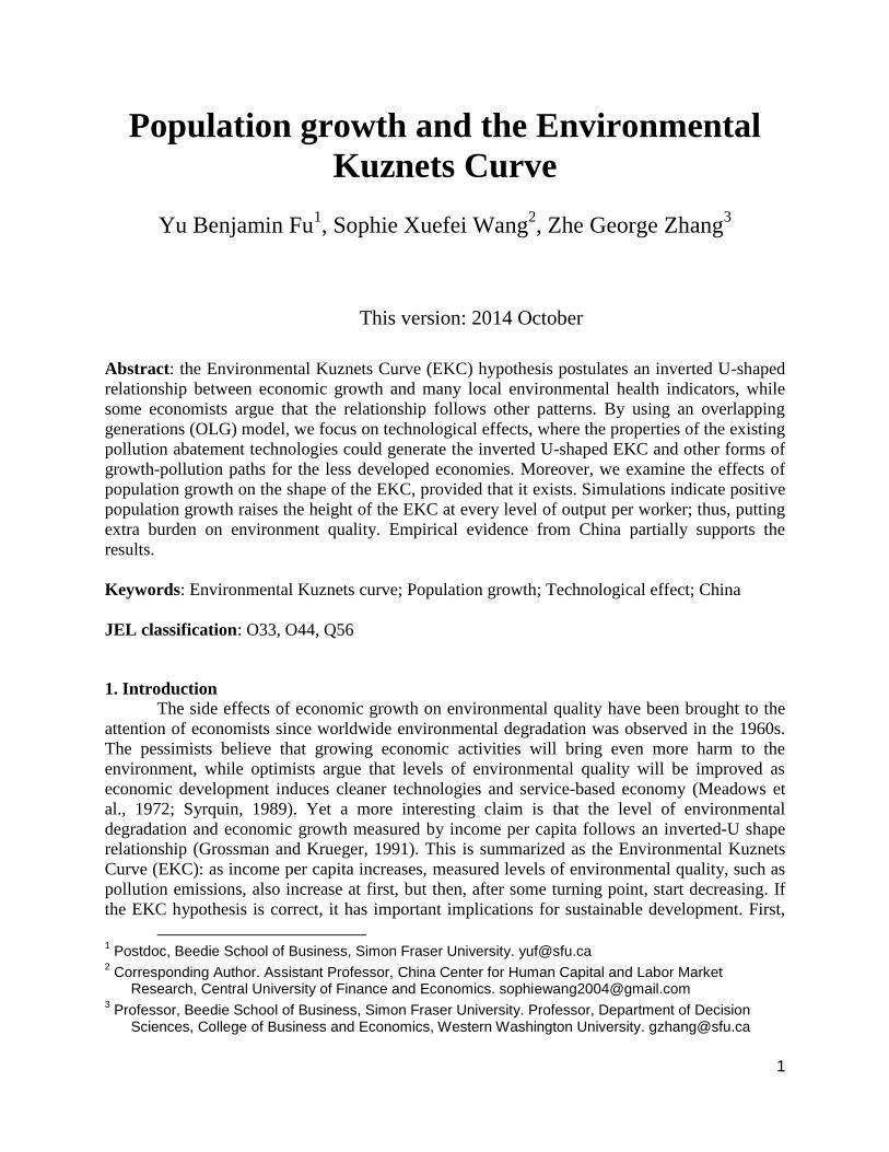
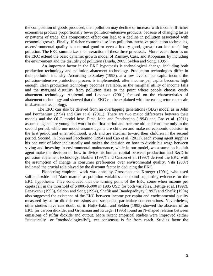
The changes in pollution and environmental quality are our focus here. Figures 3 and 4

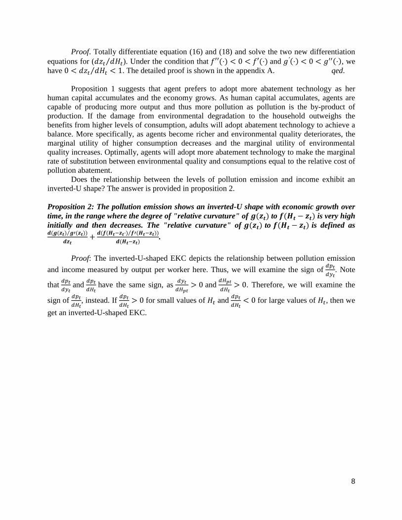
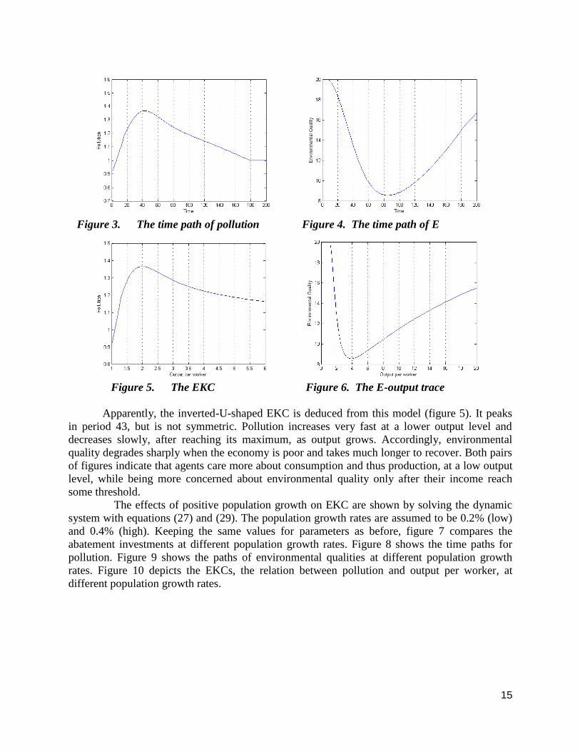
show the time paths for pollution and environmental quality. Figures 5 and 6 show the changes

in pollution and environmental quality against the output level.

15

Figure 3. The time path of pollution Figure 4. The time path of E

Figure 5. The EKC Figure 6. The E-output trace

Apparently, the inverted-U-shaped EKC is deduced from this model (figure 5). It peaks

in period 43, but is not symmetric. Pollution increases very fast at a lower output level and

decreases slowly, after reaching its maximum, as output grows. Accordingly, environmental

quality degrades sharply when the economy is poor and takes much longer to recover. Both pairs

of figures indicate that agents care more about consumption and thus production, at a low output

level, while being more concerned about environmental quality only after their income reach

some threshold.

The effects of positive population growth on EKC are shown by solving the dynamic

system with equations (27) and (29). The population growth rates are assumed to be 0.2% (low)

and 0.4% (high). Keeping the same values for parameters as before, figure 7 compares the

abatement investments at different population growth rates. Figure 8 shows the time paths for

pollution. Figure 9 shows the paths of environmental qualities at different population growth

rates. Figure 10 depicts the EKCs, the relation between pollution and output per worker, at

different population growth rates.

16

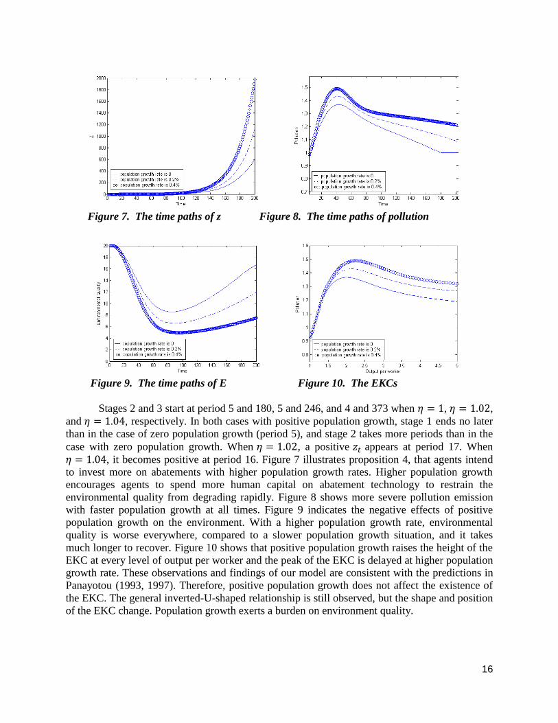
Figure 7. The time paths of z Figure 8. The time paths of pollution

Figure 9. The time paths of E Figure 10. The EKCs

Stages 2 and 3 start at period 5 and 180, 5 and 246, and 4 and 373 when , ,

and , respectively. In both cases with positive population growth, stage 1 ends no later

than in the case of zero population growth (period 5), and stage 2 takes more periods than in the

case with zero population growth. When , a positive appears at period 17. When

, it becomes positive at period 16. Figure 7 illustrates proposition 4, that agents intend

to invest more on abatements with higher population growth rates. Higher population growth

encourages agents to spend more human capital on abatement technology to restrain the

environmental quality from degrading rapidly. Figure 8 shows more severe pollution emission

with faster population growth at all times. Figure 9 indicates the negative effects of positive

population growth on the environment. With a higher population growth rate, environmental

quality is worse everywhere, compared to a slower population growth situation, and it takes

much longer to recover. Figure 10 shows that positive population growth raises the height of the

EKC at every level of output per worker and the peak of the EKC is delayed at higher population

growth rate. These observations and findings of our model are consistent with the predictions in

Panayotou (1993, 1997). Therefore, positive population growth does not affect the existence of

the EKC. The general inverted-U-shaped relationship is still observed, but the shape and position

of the EKC change. Population growth exerts a burden on environment quality.

17

5. Empirical Evidence

In this section, we use ten-year panel data from China to examine the EKC hypothesis

and the effects of population growth has on it, if it exists.8 We examine pollutants that are

supposed to have local effects (i.e., sulfur dioxide, waste water, and industrial waste gas), to

check for evidence of the EKC in China's economic development.9 We examine the possible

effects from population growth on the EKC, if it is indeed present. The ten-year panel data for

these three pollutants are compiled with other critical variables for China's 30 provinces and

metropolises, from 2000 to 2009. The data is based on China's statistical yearbooks, from 2001

to 2010.10

The yearly averages of the key variables are presented in Table D1, shown in the

appendix D.

In the traditional model, where pollution is assumed to be a by-product of the production

process, simple polynomial forms are widely used. EKC models usually use a simple reduced-

form quadratic function, sometimes with polynomial terms for the income variable, and

sometimes including the cubic level is also included in the reduced form. To examine the effects

of local population growth, dummy variables are used for six different regions. Let be the

yearly emission of the pollutant in province , at time . The following equation specifies a

possible form of the EKC model with population growth.

(35)

where is GDP per capita, is aggregate employment, is aggregate physical capital

investment, is aggregate abatement investment, and is population density. and

, where is the birth rate, is the

dummy variable for six different regions in China: represents the North; represents

the Northeast, represents the East, represents the South, represents the

West and represents the Center. indexes provinces and metropolises, and

indexes time periods. The intercept is allowed to change across regions to

capture the effects of other regional factors on local pollution over time. The EKC hypothesis

would be supported if and . The impacts of local population growth can be

examined by looking at the values of the coefficients for and , which, when

combined, change the curvature of EKC . We use fixed effects transformation to eliminate the

unobserved effect from the constant terms, Define , , and so on.

The general time-demeaned equation for each , which is estimated by pooled OLS, is:

(36)

The output of the pooled OLS regression is shown in Table 1.

8 We understand that the time span of 10 year may be too short to test a growth model. But our focus

here is to test the effect of population growth rate on the EKC, rather than to test the validity of the OLG model.

9 The pollutants that we studied include sulfur dioxide, waste residuals, industrial soot, industrial dust,

waste water, COD in water and waste gas. We choose to report sulfur dioxide, waste water and waste gas because the evidence of the EKC is strong, with significant effects from population growth.

10 China has 31 provinces and metropolises, and our data excludes Tibet because of missing data. The

consolidated data can be found at: www.sfu.ca/~yuf/research/datafile.xlsx

18

Table 1. The output of the fixed-effect model for three pollutants Variables Sulfur dioxide Waste water Waste gas

GDP per capita

GDP per capita squared

Investment

Employment

Abatement

Population density

DBYNorth

DBYNortheast

DBYEast

DBYSouth

DBYWest

DBYCenter

DBY2North

DBY2Northeast

DBY2East

DBY2South

DBY2West

DBY2Center

F value

Turning point (1000RMB)

Note: and , where is the birth rate, is the

dummy variable for six different regions in China. The coefficient with *, ** and *** is significant at 1%,

5% and 10% respectively.

The P-values for all F-tests are approximately 0.0000, which suggests overall

significance for all three estimations. Furthermore, the significant positive β and negative β

from all three estimations indicate very strong evidence of EKCs for sulfur dioxide, waste water,

and industrial waste gas in China. The turning points vary from 20,706 to 24,670 RMB for sulfur

dioxide; from 13,501 to 14,523 RMB for waste water; and from 8,480 to 12,269 RMB for

industrial waste gas.11

Nevertheless, the effects of population growth are not significant for all

regions.12

For sulfur dioxide, only the coefficients of the dummy variables for the West are

significant. For waste water, the coefficients of the dummy variables for the North, the South,

and the East are significant. For industrial waste gas, the coefficients of the dummy variables for

the North, the Northeast, and the East are significant.

The effects of population growth are not significant for all regions. Figures 11, 12, and

13 show the effects of population growth for regions with significant coefficients.

11

The real GDP per capita in China varies among different regions. In 2000 the range was from 3,127 to 33,863 RMB, and the national GDP per capita was 8,846 RMB. In 2009 the range was from 6,681 to 61,251 RMB and the national GDP per capita was 20,757 RMB. The base year is 1997.

12 To be consistent in our model, we used birth rate to approximate population growth.

19

Figure 11. The EKCs of sulfur dioxide

Figure 12. The EKCs of waste water Figure 13. The EKCs of waste gas

From these three figures we can still observe EKCs with positive population growth. The

solid curves are the benchmarks. When income level is low, the pollution emissions rise faster

with positive population growth for sulfur dioxide at the increasing part of the EKC. For the

other two pollutants, the effects of positive population growth are different. We observe faster

rising EKCs at low income levels in some regions (the East for waste water and the North for

waste gas), which is consistent with proposition 6. Nevertheless, we also observe some slower

rising EKCs at low income levels in the other regions, where positive population growth rates are

also significant. Not surprisingly, the shape of the EKC is determined by industry-specialized

production technology, abatement technology, the relative growth rate of population to human-

capital accumulation, and so on; but the population growth rate has an effect on the EKC.

6. Concluding Remarks

In this paper, we use an overlapping generations (OLG) model to study the EKC, an

inverted-U-shaped relationship between environmental degradation measured by environmental

health indicators and income. In out OLG model, the representative agent is altruistic toward her

children, and must balance her household consumption with investments in pollution abatement

20

technology. The investment increases monotonically as the economy becomes rich. The relative

improvement of the abatement technology to the production technology is mathematically

expressed as the degree of "relative curvature" of to , and it determines the shape of the

curve for the relationship between pollution and economic growth. When the "relative curvature"

of to is initially very high, and then decreases, the inverted-U-shaped EKC is observed.

Population growth is not neutral and has two effects of opposite directions on the EKC. On one

side, more children in the household means more consumption, and thus production, which

generates more pollution. On the other side, agents may have more incentive to reduce the level

of pollution emission, since pollution negatively affects their children’s welfare and thus their

utility. These two effects have impacts on the pollution path, though the inverted-U-shaped EKC

is still present. The assumption about the self-adjustment ability of the environment is critical for

obtaining the result that the environmental quality path will be U-shaped and then return to its

original stable level. Simulations confirm the propositions and clearly indicate that the EKC is

deduced under the given assumptions of our model. Moreover, simulations display the effects of

positive population growth on the EKC and environmental quality: the height of the EKC is

raised at every level of output per worker and environmental quality is made worse everywhere

and the peak of the EKC shifts to the right. Empirical evidence from China support the EKC

hypothesis and provide partial support for the predictions of our model regarding the effect of

population growth on the EKC. Higher population growth rate shifts the EKC curve upwards and

faster rising EKCs can be observed at low income levels with higher population growth rate in

some regions.

References

Anderoni, J., Levinson, A., 2001. The simple analytics of the environmental Kuznets curve.

Journal of Public Economics. 80, 269-286.

Arrow, K., Bolin, B., Costanza, R., Dasgupta, P., Folke, C., Holling, C. S., Jansson, B-O., Levin,

S., Maler, K-G., Perrings, C., D. Pimentel, 1995. Economic growth, carrying capacity,

and the environment. Science. 268: 520-521.

Barbier, E B. 1997. Introduction to the environmental Kuznets curve special issue. Environment

and Development Economics. 2: 369-381.

Cao, D., Wang, L., Wang Y., 2011. Endogenous fluctuations induced by nonlinear pollution

accumulation in an OLG economy and the bifurcation control. Economic Modelling, 28,

2528-2531.

Carson, R, McCubbin R., 1997. The relationship between air pollution emissions and income:

US data. Environment and Development Economics. 2, 433-450.

Caviglia-Harris, J., Chambers, D., Kahn, J., 2009. Taking the "U" out of Kuznets: A

comprehensive analysis of the EKC and environmental degradation. Ecological

Economics. 68, 1145-1155.

Cole, M. A., A. J. Rayner, and J. M. Bates, 1997. The Environmental Kuznets Curve: An

Empirical Analysis. Environment and Development Economics, 2(4): 401–16.

Cropper, M., Griffiths, C., 1994. The interaction of population growth and environmental

quality. American Economic Review, 84(2), 250-254.

Dinda, S., 2005. A theoretical basis for the environmental Kuznets curve. Ecological Economics,

53, 403-413.

Grossman, G.M., Krueger, A.B., 1991. Environmental impacts of a North American Free Trade

Agreement. NBER, working paper 3914, Cambridge, MA.

21

Grossman, G.M., Krueger, A.B., 1995. Economic growth and the environment. Quarterly Journal

of Economics, 110(2), 353-377.

Hettige, H., Robert E. B. Lucas, and D. Wheeler, 1992. The Toxic Intensity of Industrial

Production: Global Patterns, Trends, and Trade Policy. American Economic Review,

82(2): 478–81.

Hilton, F.G.H., Levinson, A., 1998. Factoring the environmental Kuznets curve: evidence from

automotive lead emissions. Journal of Environmental Economics and Management. 35,

126-141.

Holtz-Eakin, D., Seldon, T.M., 1995. Stoking the fries? CO emissions and economic growth.

Journal of Public Economics. 57, 85-101.

John, A., Pecchenino, R., 1994. An overlapping generations model of growth and the

development. The Economic Journal. 104, 1393-1410.

Koop, T., Tole, T., 1999. Is there an environmental Kuznets curve for deforestation? Journal of

Development Economics. 58, 231-244.

Koren'kov, VN., 1991. Biological purification of sewage from chemical plants. Russian

Chemical Reviews. 60, 273.

Lopez, R., 1994. The environment as a factor of production: the effects of economic growth and

trade liberalization. Journal of Environmental Economics and Management. 27, 163-184.

Martinez-Zarzoso, I., Maruotti, A., 2011. The impact of urbanization on CO2 emissions:

Evidence from developing countries. Ecological Economics. 70(7), 1344-1353.

Meadows, D. H., D. L. Meadows, J. Randers, W.W. Behrens, 1972. The Limits to Growth. Earth

Island Limited, London.

Munasinghe, M., 1999. Is Environmental Degradation an Inevitable Consequence of Economic

Growth: Tunneling Through the Environmental Kuznets Curve. Ecological Economics.

29(1), 89–109.

Nguyen, V., 2002. Endogenous population and environmental quality. Working papers of BETA.

Panayotou, T., 1993. Empirical tests and policy analysis of environmental degradation at

different stages of economic development. International Labor Organization working

paper 238, Geneva, Switzerland.

Panayotou, T., 1997. Demystifying the environmental Kuznets curve: Turing a black box into a

policy tool. Environment and Development Economics. 2, 465-484.

Roy N., Van Kooten C., 2004. Another look at the income elasticity of non-point source

pollutants: a semi parametric approach, Economic letters. 85(1), 17-22.

Seldon, T.M., Song, D., 1994. Environmental air quality and development: is there a Kuznets

curve for air pollution emissions. Journal of Environmental Economics and Management.

27, 147-162.

Seldon, T.M., Song, D., 1995. Neoclassical growth, the J cuve for abatement, and the inverted-U

curve for pollution. Journal of Environmental Economics and Management. 29, 162-168.

Shafik, N., 1994. Economic development and environmental quality: An econometric analysis.

Oxford Economic Papers. 46, 757-777.

Shafik, N., S. Bandyopadhyay, 1992. Economic Growth and Environmental Quality: Time Series

and Cross Section Evidence. Working paper. World Bank, Washington, DC..

Song, T., Zheng, T., Tong, L., 2008. An empirical test of the environmental Kuznets curve in

China: A panel cointegration approach. China Economic Review. 19, 381-392.

Stern, D., 2004. The rise and fall of the environmental Kuznets curve. World Development. 32,

1419-1439.

22

Stokey, N., 1998. Are there limits to Growth? International Economic Review. 39(1), 1-31.

Syrquin, M., 1989. Patterns of structural change. In: Chenery, H., Srinivasan, T.N. (Eds.),

Handbook of Development Economics. Elsevier, Amsterdam, 203–273.

Vincent, J., Ali, R.M., 1997. Environment and Development In a Resource-Rich Economy:

Malaysia Under the New Economic Policy. Harvard Institute for International

Development, Harvard University.

Vita, G., 2007. Is the discount rate relevant in explaining the environmental Kuznets curve?

Journal of Policy Modeling. 30, 191-207.

Wagner, M., 2008. The carbon Kuznets curve: A cloudy picture emitted by bad econometrics?

Resource and Energy Economics. 30, 388-408.

Wang, C., Fang, Y., Wu, X., Hu, D., Zuo Z., Li C., Xu Y., Xiao, G., 2006. Research on the

ability of twenty- one ornamental plants to absorb and purify environmental pollutants. Journal

of Shandong Forestry Science and Technology. 6, 11-13.

Appendices

Appendix A: proof of proposition 1

From equation (12) and (13), . Combining with equation (17), we have

(A1)

From equation (12) or (13) and (14), we have

(A2)

(A3)

Substitute equations (A2) and (A3) into equation (15), we have equation (18). Totally

differentiating equation (18) gives

(A4)

where

All the terms in are positive and all the terms in are

negative, under the assumption that and .

Totally differentiating equation (16) gives

(A5)

Solving the equation system of (A4) and (A5) by eliminating gives

23

(A6)

Each term in the numerator and the denominator of (A6) is positive, under the assumption that

and . Thus, . qed.

Appendix B: Proof of proposition 3

If the economy starts from its natural equilibrium , from equation (16) the environmental

quality at time is:

i.e.,

(B1)

(B2)

(B3)

When , we also have:

(B4)

This implies that the trace of is totally opposite to that of . Since is inverted-U-shaped,

is then be U-shaped and reaches its minimum point when goes to the maximum.

If :

(B5)

Because in stage two , the environmental quality will then degrade at all times in this

stage. At the end of this period which means reaches its minimum at this time

because it will start to improve in stage three.

If :

(B6)

Because in stage two we have:

Also, if when in stage two:

Therefore is bounded between ( , ). When is

increasing, which implies then is deceasing over time, even after reaches its

maximum. But at the end of stage two, and . This indicates is already

increasing. Because is monotonically decreasing after reaching its maximum point, the

minimum of must appear sometime between the time when reaches its maximum and the

end of stage 2. qed.

Appendix C: Proof of proposition 5

From equation (20) and (21), we have . In combination with (22), (23), and

(25), we have:

24

(C1)

Totally differentiating (C1), we have:

(C2)

where

Solving the equation system containing (C2) and (A5), we have:

(C3)

where

Because both the denominator and numerator of (C3) are positive, and the numerator is smaller

than the denominator, we have .

Equation (C3) shows that if there is no population growth. Because , we know that:

Therefore the relationship between and decides which is bigger, either

that in (A4) or that in (C3). we know that:

(C4)

where is the product of the two denominators, and , and it is positive. Therefore

is positive, as in equation (17). Because before pollution

emission reaches its maximum, this implies with positive population growth is smaller

than without population growth. After the economy becomes rich and pollution emission starts

to decrease, with positive population growth will be greater than without population

growth. qed.

25

Appendix D

Table D1. The yearly averages of the panel data Province sulfur

dioxide

(ton)

Waste

water

(10000

ton)

Gas

(100

millio

n m3)

GDP

Per

capita

(10000

RMB)

Real

Invest

ment

(100

million

RMB)

Emplo

yment

(10000)

Real

abatement

(10000

RMB)

Population

density

(per km2)

Popula

tion

growth

rate

( 0/00 )

Beijing 115087 16607 3711 2.5406 2258.5 865 65612 891.3821 1.58

Tianjin 209474 21078 3986 2.6852 1453.9 445 96314 881.2472 1.92

Hebei 1188256 112227 25406 1.1906 3888.7 3499 119814 359.7127 5.64

Shanxi 1047918 36474 14094 0.8786 1454.8 1486 173371 210.2571 6.23

Inner

Mongolia

970855 24189 12223 1.1389 1865 1051 64963 20.00311 4.42

Liaoning 823598 96849 18235 1.6546 3610 1948 174795 284.469 1.6

Jilin 255672 36568 4529 1.0801 1690.5 1116 47682 143.5528 2.79

Heilongjiang 329913 46556 5743 1.3672 1609.5 1664 74099 83.44418 2.76

Shanghai 331362 60637 7928 4.1033 2896.8 790 64901 2657.896 0.62

Jiangsu 1139960 250812 17443 2.0199 6348.4 3896 210428 720.6637 2.43

Zhejiang 696351 167948 11758 2.1349 5009.6 3098 147119 466.3847 4.17

Anhui 438846 65720 7937 0.8297 2414.8 3481 56306 443.422 6.24

Fujian 313492 100127 5602 1.8119 2362.9 1828 125670 284.3904 5.53

Jiangxi 415291 53672 4238 0.7965 1741 2072 32119 254.5905 7.78

Shandong 1543785 134086 21083 1.6322 6426.7 5031 375634 580.3073 4.85

Henan 1070006 117298 13540 0.8806 3858.3 5573 127124 563.1387 5.46

Hubei 555634 99408 8417 1.1839 2473.1 2720 100779 312.6937 3.09

Hunan 673323 111594 5989 0.9085 2103.1 3621 70732 304.9056 4.79

Guangdong 1010679 168215 12915 1.877 5587.2 4508 218847 462.315 7.79

Guangxi 812124 125282 8252 0.8153 1587.4 2645 66175 199.9296 7.4

Hainan 21706.3 6954.9 759.4 0.9688 332.27 368 4117.7 226.8859 9.04

Chongqing 627432 75315 4645 0.9118 1569.8 1697 33978 359.9889 3.37

Sichuan 957149 112388 9252 0.7944 3095.3 4596 105907 172.5918 3.57

Guizhou 718105 17565 5413 0.4065 857.34 2148 40691 212.1471 8.68

Yunnan 377304 35048 5214 0.6691 1390.8 2437 50192 109.9928 8.31

Shaanxi 693357 37854 5088 0.7228 1588.5 1878 57730 178.0309 4.26

Gansu 393161 20490 4143 0.5852 733.4 1294 62259 56.42585 6.53

Qinghai 73777 5142.7 1581 0.7798 285.13 260 5722.1 7.361878 9.9

Ningxia 255691 14345 2549 0.7217 336.87 292 26829 86.63381 10.3

Xinjiang 325396 18305 3921 0.9764 1024.5 741 37889 11.592 10.5

Note: All provinces of China are divided into six regions. The North includes Beijing, Tianjin, Hebei, Shanxi and

Inner Mongolia; the Northeast includes Liaoning, Jilin and Heilongjiang; The East includes Shanghai, Jiangsu,

Zhejiang, Anhui, Fujian, Jiang xi and Shandong; The South includes Henan, Hubei, Hunan, Guangdong, Guangxi

and Hainan; The West includes Chongqing, Sichuan, Guizhou and Yunnan; The center includes Gansu, Qinghai,

26

Ningxia and Xinjiang.

All numbers are yearly averages, from 2001 to 2010.

GDP per capita, investment and abatement spending are in real terms. The base year is 1997.

Data source: China's statistical yearbooks, 2001 to 2010.