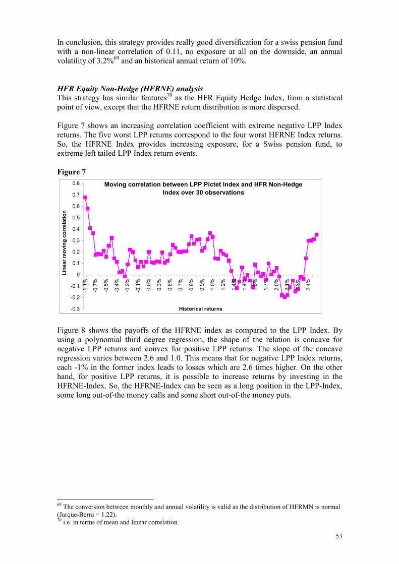
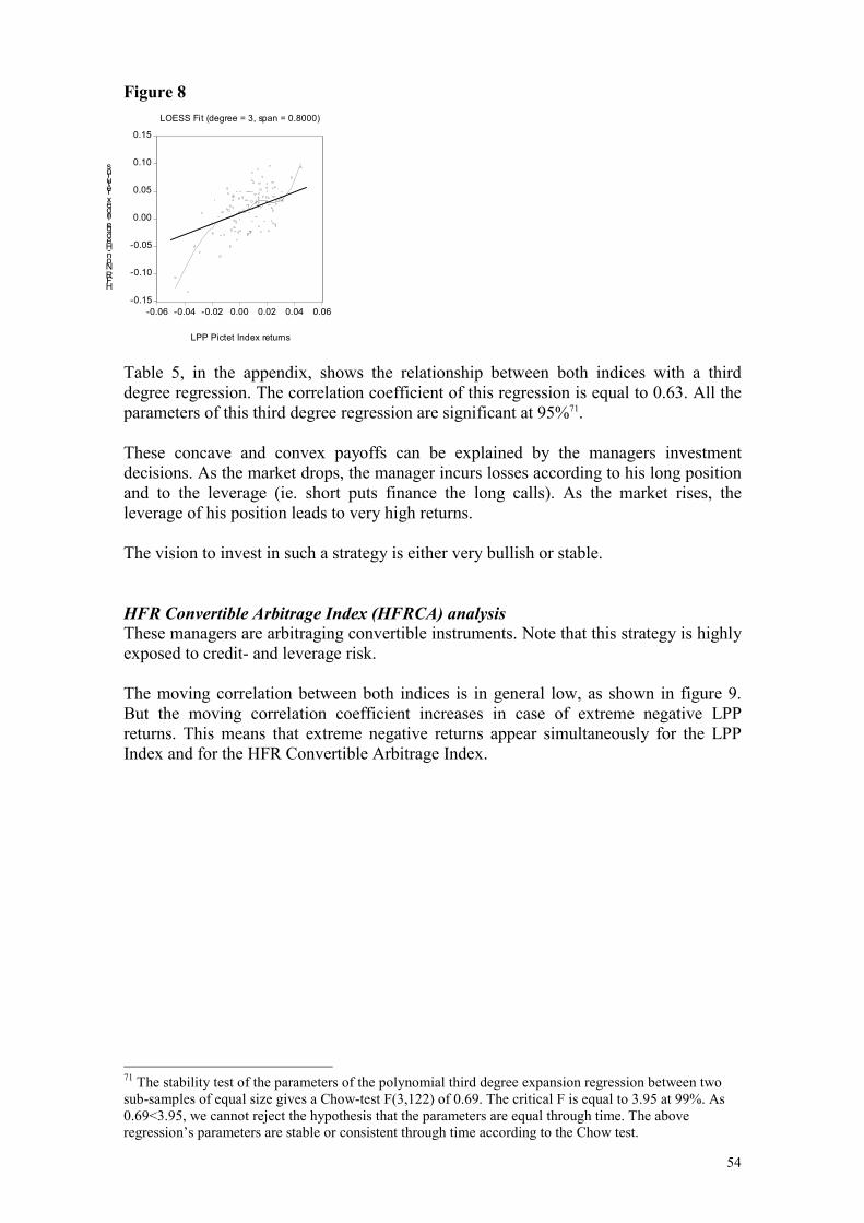
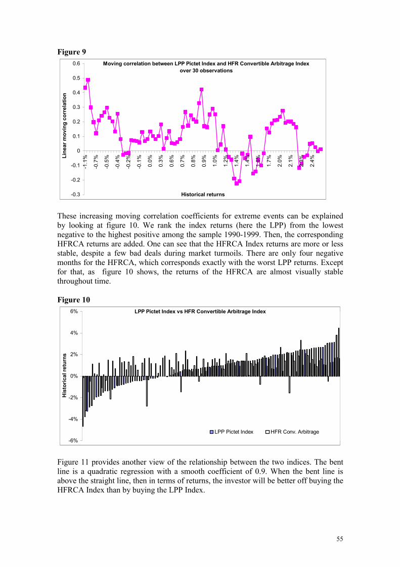
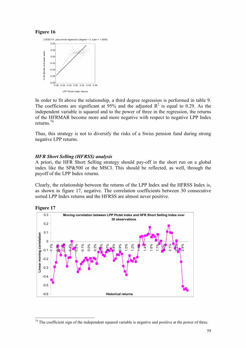
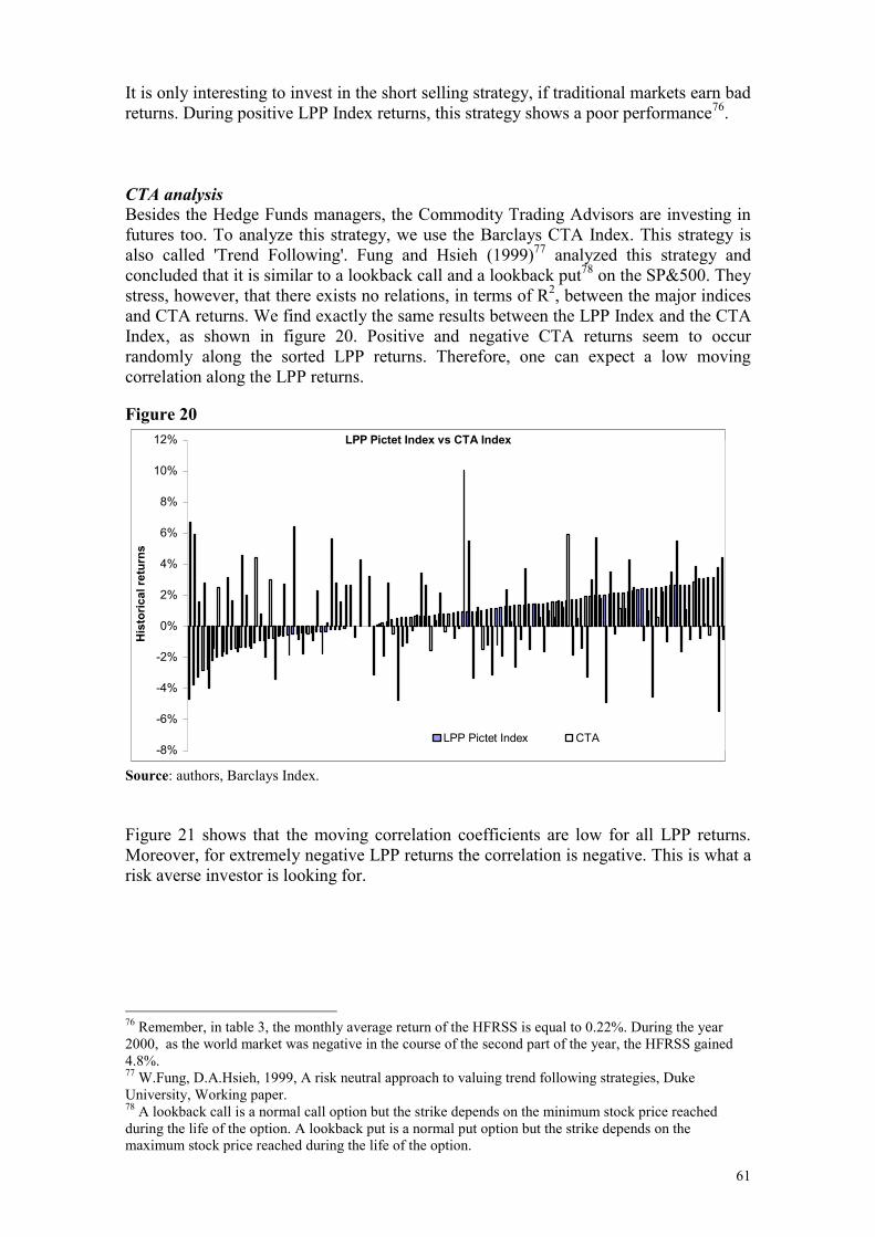
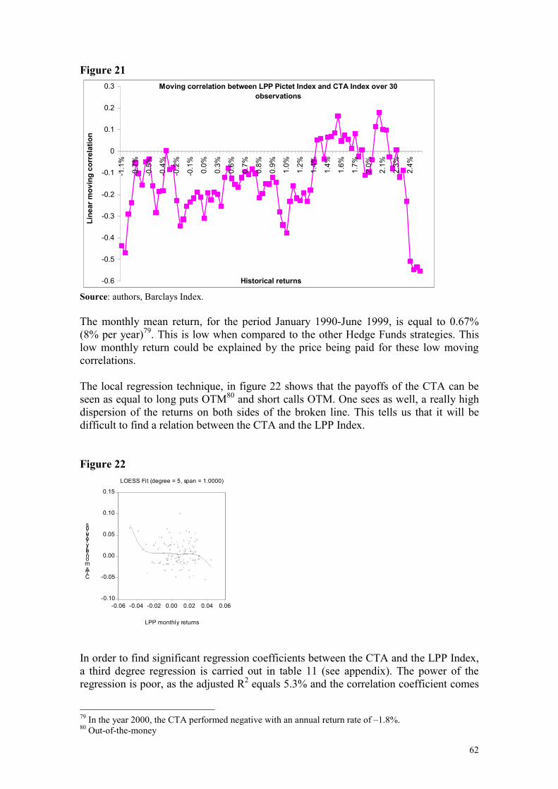
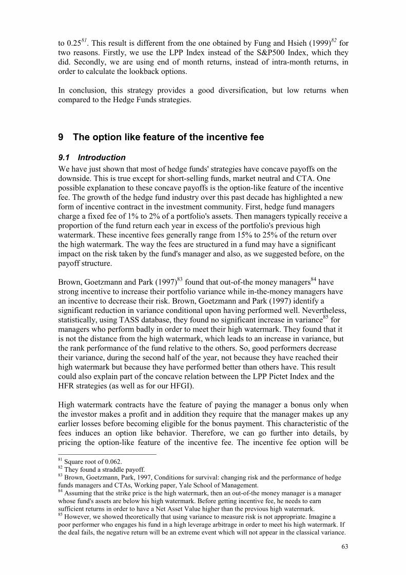
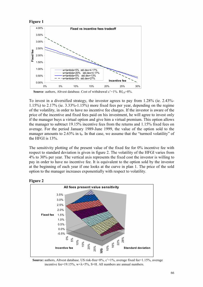
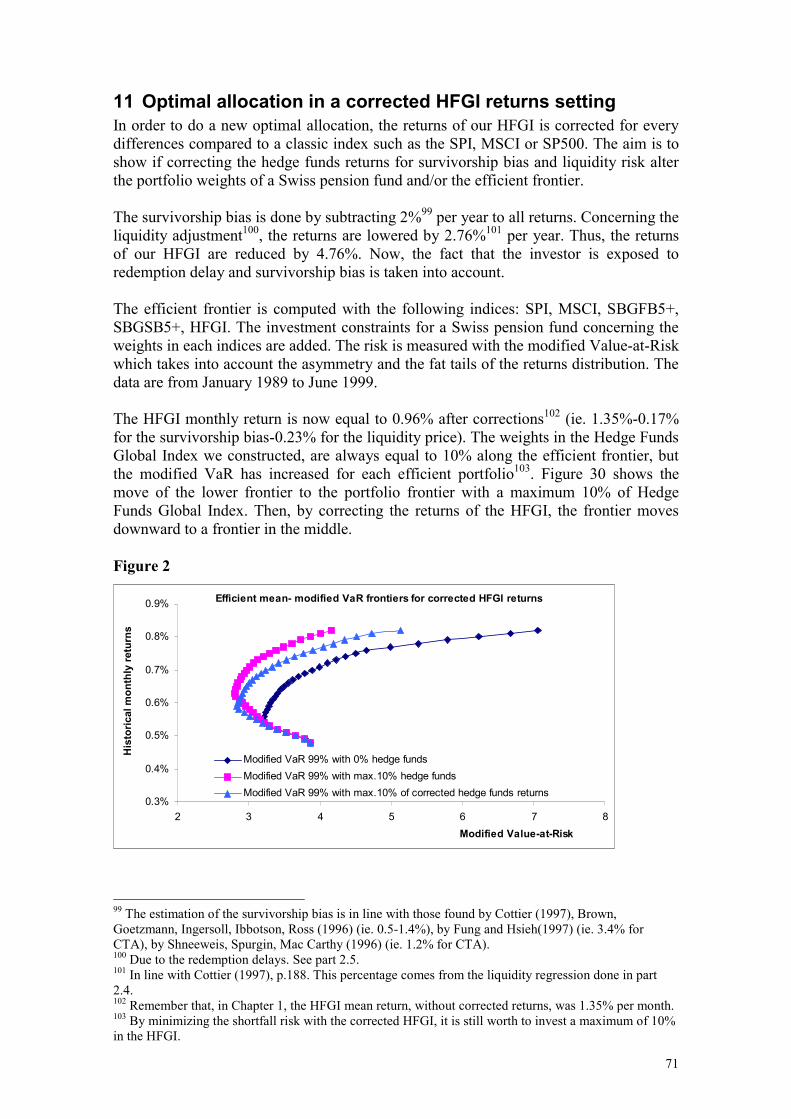
1 Portfolio Allocation with Hedge Funds Case study of a Swiss institutional investor First version: January 2000 This version: August 2004 Laurent Favre José-Antonio Galeano CEO & Founder AlternativeSoft LLC Banque Cantonale Vaudoise Switzerland Switzerland Abstract Asset allocation advisers usually use the mean-variance framework to show the benefits of investing in hedge funds. We prove that this is not optimal and develop a method based on a modified Value-at-Risk model for non-normally distributed assets: we called it modified VaR. We take the example of a Swiss pension fund investing part of its wealth in hedge funds. We also use a shortfall risk approach and show that investing in a diversified Hedge Funds portfolio is beneficial for lowering its modified Value-at-Risk. We find that constructing a portfolio without taking into account skewness and kurtosis underestimates the portfolio risk, measured with our developed modified VaR, by 10% to 40% depending on the level of historical return. Then, we analyze the distribution of Hedge Funds strategies returns, the average returns obtained over the past ten years and their correlation with a traditional portfolio. We show that the classical linear correlation and the classical linear regression cannot be relied upon hedge funds. Moreover, we will show that only three strategies, Convertible Arbitrage, Market Neutral and CTA, give diversification during market downturns. The techniques used are non-linear regressions, moving correlation and local correlation. Finally, we corrected the returns of our hedge funds index for survivorship bias and liquidity risk and find that it is still beneficial to invest in a well diversified hedge funds portfolio. Adding 10% of hedge funds in a swiss pension fund portfolio lowers the risk in a mean-variance world by 3% to 35%. In a corrected modified Value-at-Risk setting, 10% of hedge funds diminishes the risk by only 0% to 20%.
Transcript
1
Portfolio Allocation with Hedge Funds
Case study of a Swiss institutional investor
First version: January 2000 This version: August 2004
Abstract Asset allocation advisers usually use the mean-variance framework to show the benefits of investing in hedge funds. We prove that this is not optimal and develop a method based on a modified Value-at-Risk model for non-normally distributed assets: we called it modified VaR. We take the example of a Swiss pension fund investing part of its wealth in hedge funds. We also use a shortfall risk approach and show that investing in a diversified Hedge Funds portfolio is beneficial for lowering its modified Value-at-Risk. We find that constructing a portfolio without taking into account skewness and kurtosis underestimates the portfolio risk, measured with our developed modified VaR, by 10% to 40% depending on the level of historical return. Then, we analyze the distribution of Hedge Funds strategies returns, the average returns obtained over the past ten years and their correlation with a traditional portfolio. We show that the classical linear correlation and the classical linear regression cannot be relied upon hedge funds. Moreover, we will show that only three strategies, Convertible Arbitrage, Market Neutral and CTA, give diversification during market downturns. The techniques used are non-linear regressions, moving correlation and local correlation. Finally, we corrected the returns of our hedge funds index for survivorship bias and liquidity risk and find that it is still beneficial to invest in a well diversified hedge funds portfolio. Adding 10% of hedge funds in a swiss pension fund portfolio lowers the risk in a mean-variance world by 3% to 35%. In a corrected modified Value-at-Risk setting, 10% of hedge funds diminishes the risk by only 0% to 20%.
3 PORTFOLIO OPTIMIZATION WITH HEDGE FUNDS............................................................ 5
3.1 INTRODUCTION OF THE MEAN-VARIANCE FRAMEWORK................................................................ 5 3.2 DATA............................................................................................................................................ 6
3.2.1 Traditional financial instruments......................................................................................... 6 3.2.2 Hedge Funds data ................................................................................................................ 7 3.2.3 Currency .............................................................................................................................. 8
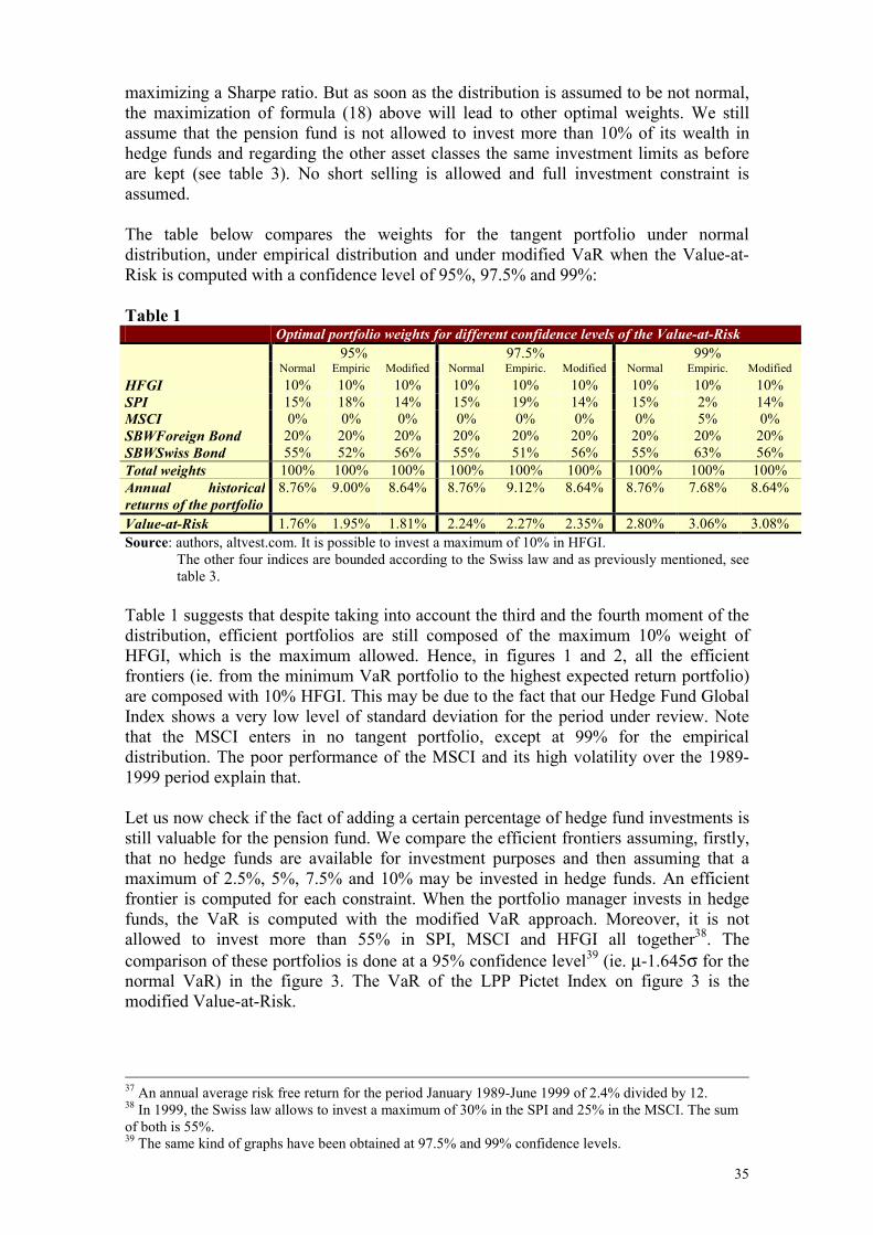
5.3 MEAN –MODIFIED VALUE-AT-RISK OPTIMIZATION..................................................................... 26 5.3.1 Introduction ....................................................................................................................... 26 5.3.2 Asset allocation in a mean-modified Value-at-Risk framework ......................................... 27 5.3.3 Efficient frontier in a mean-modified Value-at-Risk setting............................................... 32 5.3.4 Conclusion ......................................................................................................................... 34
5.4 OPTIMAL TANGENT WEIGHTS IN A MEAN-MODIFIED VAR SETTING............................................. 34 5.5 VERIFYING THE ROBUSTNESS OF THE RESULTS OBTAINED .......................................................... 37
5.5.1 Efficient frontiers with the HFR Index ............................................................................... 37 5.5.2 Out-of-Sample in a mean-modified VaR setting................................................................. 39
6 ALLOCATION IN A DOWNSIDE-RISK SETTING .................................................................. 40
1 Introduction Switzerland both has three pillar retirement system. The AVS is a basic Sate pension plan, financed by employees and employers. A complementary scheme came into force on 1 January 1985 with the introduction of the LPP, "Loi sur la prévoyance professionnelle". The LPP contains the Swiss Federal guidelines for retirement provisions. And finally, there are supplemental schemes corresponding to private provisions for individuals. With the introduction of the LPP in January 1985, Swiss pension funds developed rapidly. In 1997, Switzerland had the third largest pension fund assets in Europe with US$233 billion in total. In 1999, pension fund assets represented US$287 billion and are expected to grow at 11% annually for the next few years1. Setting investment decisions for Swiss pension funds is a major challenge for several reasons. Obviously, the investments should provide with a long term rate of return, which is in line with the liability structure of the pension plan. Furthermore, the investment decisions should comply with the legal requirement of the LPP. This law standardized existing Cantonal pension fund regulations regarding asset categories and their maximum authorized weightings. It also requires that assets held by pension funds show a minimum rate of return of 4% per annum. Over the last few years, pension funds have had no difficulty in achieving their target return. They have benefited from the high level of interest rates. Nevertheless, from this point of view, future returns look more problematic. Although many pension funds have enjoyed the bull run of the equity market, the impact of falling interest rates is more important for some of them and is twofold: Firstly, it reduces the rate of return obtained from the assets invested. This reduction may be important as Swiss pension funds traditionally invest heavily in bonds. Secondly, due to the decrease of the actualization of the interest rate, it resulted in increasing the liability side of the balance sheet and thus, ate up part of the surpluses accumulated over the last decade. Swiss pension funds are not the only ones to be concerned by these changing market conditions. For example in the UK, around 25% of the pension funds which responded to a National Association of Pension Funds survey have a surplus of less than 10%, a level which put them at risk of becoming under funded2. Aware of this state of fact, an increasing number of pension funds started looking at alternative investments. Alternative Investments are a class of financial vehicles including Hedge Funds, Managed Futures and Private Equity. Another reason for pension funds to start looking at this type of financial instruments stems from their diversification benefits. Solnik (1974)3 was one of the first economists to document the benefits of an international diversification. Investing internationally offers benefits in terms of portfolio risk reduction and return enhancement. Odier, Solnik and Zucchinetti (1995)4 show in their paper that a Swiss pension fund should engage in extensive international asset allocation. In this context, pension funds are looking for new financial instruments, which have a low coefficient of correlation with traditional
1 Source: Intersec 2 Media Release, Credit Suisse Asset Management. 3 Bruno Solnik, 1974, Why not diversify internationally rather than domestically ?, Financial Analyst Journal 30, 48-54. 4 Patrick Odier, Bruno Solnik and Stephane Zucchinetti, 1995, Global Optimization for Swiss Pension Funds, Finanzmarkt und Portfolio Management, Nr. 2
5
instruments in all market conditions. Odier and Solnik (1993)5 show that even if there is little evidence that either stock or bond markets have become more correlated or volatile worldwide, it appears that correlation increases when market volatility increases, that is precisely when the diversification potential offered by low correlation is most needed. This master's thesis has three objectives. First, we analyze the benefits for a Swiss pension fund to invest part of its wealth in hedge funds. We also highlight the weaknesses of the mean-variance theory and its limitations (when we start dealing with this type of financial instruments). Then, we analyze some hedge funds' characteristics like their payoffs and fee structure. Finally, we attempt to show that part of the excess return faced by hedge funds is nothing else than a compensation for taking specific risks. We analyze in particular the case of liquidity risk.
2 Introductory comments Before analyzing the allocation of the portfolio assets of a pension fund, it is necessary to understand its investment objectives. These objectives simultaneously depend on the assets of the fund and on the level of its liabilities, which consist of all the benefits that will have to be paid to the contributors in the future. A clear assessment of the pension liabilities should be used to set the objectives of the asset allocation policy. This is more generally called an Asset and Liability Management (ALM) approach. An important factor influencing the level of liabilities and assets is the way employees' contributions are calculated. Swiss law knows two mechanisms, the defined benefit plan and the defined contribution plan. According to Odier, Solnik and Zucchinetti (1995), the ALM approach for a pension fund with a defined benefit plan ought to be to minimize the risk for the return on invested assets will be below the rate of wage inflation affecting the pension liabilities. In the case of a defined contribution plan, the ALM approach should be to achieve the best long term real return on invested assets. After a brief introduction on the framework on which the analysis is done, we look at the impact on the efficient frontier of investing part of the assets' portfolio in hedge funds. Then, we perform an out-of-sample analysis. At this stage, it is important to check if the implicit assumptions underlying the conceptual framework are respected when dealing with hedge fund instruments. We finally introduce a Value at Risk and a shortfall risk approach in order to reassess the benefits for a Swiss pension fund to invest in this type of instruments.
3 Portfolio optimization with Hedge Funds
3.1 Introduction of the mean-variance framework Markowitz identified the trade-off faced by an investor. Investment decisions are made to achieve an optimal risk/return tradeoff from the available opportunities. In order to meet this objective, the portfolio manager must first evaluate capital market information
5 Patrick Odier and Bruno Solnik, 1993, Lessons for International Asset Allocation, Financial Analyst Journal March-April 1993.
6
and quantify ex-ante measures of both risk and expected return for the appropriate set of assets. Thus, he has to isolate those combinations of assets that are the most efficient, in order to provide the lowest level of risk for a desired level of expected return. He, then, has to select one combination that is consistent with the risk aversion of the investor. While the principle of identifying portfolios with the required risk and return characteristics is certainly clear, the appropriate definition of risk is more ambiguous. Risk may be defined differently according to the sensibility and the objectives of the portfolio manager. One manager might view risk as the probability of shortfall below some benchmark level of return, while another may be more sensitive to the overall magnitude of a loss. Mean-variance analysis has been increasingly applied to asset allocation and it is now the traditional formulation of the investment decision problem. In order to achieve the most efficient portfolio, assets are combined so as to minimize the variance for a given level of return. Here, risk is defined as the variance or standard deviation of the portfolio. Standard deviation of the returns is the most traditional statistical measure for risk. It corresponds to the dispersion of the returns around the mean return. The main justification for using the mean-variance formulation is its tractability, as it requires relatively limited data. Instead of using the full assets returns' distribution, we summarize it by its two first moments, that is the mean and the variance of the returns:
where R is the return of the asset. It is interesting to observe the importance of the first period model on which the mean and the variance are estimated given the underlying hypothesis of the framework. Regarding this last point, a detailed analysis is done in the next section.
3.2 Data
3.2.1 Traditional financial instruments We first replicate a traditional Swiss pension fund's portfolio. For that purpose, we select the Swiss Performance Index as a proxy for the investments in Swiss stocks. For the investments in Swiss bonds, we select the Lehman Brothers Swiss Bond Index. For the foreign investments, we use the Morgan Stanley Capital Index World (MSCI) for the stocks and the Lehman Brothers weight Global Bond Index for the bonds. We do not include investments in Swiss or foreign real estate even if pension funds are allowed to invest part of their wealth in these instruments. Real estate indices with enough historical data are not available on the market. We use monthly data over a period of almost ten years, that is from January 1989 to June 1999.
( )
=Ε= ∑=
N
iiR
NRMean
1
1
( )( )[ ]2)( RRRVarVariance Ε−Ε==
)(tan RVariondardDeviatS =
(1)
(2)
(3)
7
3.2.2 Hedge Funds data Hedge fund indices sold by the biggest companies like Managed Accounts Reports, Inc.(MAR), Hedge Fund Research, Inc.(HFR) or Evaluation Associates Capital Market (EACM) differ widely in purpose, composition and in the way they are constructed. In short, the MAR and HFR indices are not replicable because their composition is not known and because they use arithmetic averaging, which requires monthly rebalancing to replicate. The EACM index is constructed to be replicable but its composition is not known. Furthermore, there is no doubt that some funds included in the indices are not anymore opened to new investors. Several studies on mutual funds have shown that fund indices may be impacted by significant bias. This is also true for hedge fund indices. Ackermann, McEnally and Ravenscraft (1999)6 develop this issue and analyze its impact on returns. In our analysis, we created our own index. The objective is to obtain an index which is replicable by investors and which is also representative of the hedge fund industry. We included the following strategies: Table1 Investment Style Number of hedge
funds selected Short only & short biased 3 Statistical arbitrage 2 Asset & mortgage 5 Convertible bond 5 Distressed securities 5 Emerging markets 1 Fixed income arbitrage 4 Global macro 4 High yield bond 1 Index & options arbitrage 4 Long-short European equity 5 Long-short International equity 2 long-short U.S. equity 5 Market neutral 2 Merger arbitrage 5 Total 53 We built an equally weighted Hedge Fund Global Index (HFGI), as it is the simplest and more objective technique. We obtain the fund's returns on a monthly basis, from January 1989 to June 1999. It is important to highlight, at this stage, that the objective is not to construct the optimal hedge fund portfolio, considering that the investor is a pension fund. Therefore, we haven't selected the funds based on their historical performances or based on their low degree of correlation with more traditional financial instruments. Hedge funds were selected based on their market capitalization in 1989, the objective being to select big caps. This selection methodology has two important advantages: Indices published by MAR, or EACM are often said to contain a survivorship bias. The performance of these indices doesn't include hedge funds that
6 Carl Ackermann, Richard McEnally and David Ravenscraft, 1999, The performance of hedge funds: risk, return and incentives, Journal of Finance.
8
went bankrupt. The index returns are therefore upwardly biased. Furthermore, they also have a self-selection bias. For example, mainly managers with good performances ask to be included in these databases. In our case, the self-selection bias is mitigated by the fact that we selected the funds on a market capitalization basis and not based on the performance. Our selection methodology is coherent with the way a pension fund would select hedge funds to include in its portfolio. One criterion for the selection of a fund consists in having a low risk of going bankrupt. Therefore, a critical size in terms of market capitalization may be determinant for a pension fund in order to select a hedge fund. To assess the features of our constructed index, let us compare it to the Hedge Fund Research Weighted Composite Index (HFRWI), published by Hedge Fund Research, Inc. Table 2
HFRWI Constructed HFGI
Average ret. 1.31 1.37 Stand.Dev. 1.93 1.12 Sharpe Ratio 0.68 1.22 From January 1990 to June 1999, our constructed hedge fund global index shows an almost similar average monthly return compared to the Hedge Fund Research Weighted Composite index . HFGI has a lower standard deviation compared to the HFRW index. Due to this difference, we decided to test, in a further section, the robustness of results, obtained with our constructed index, by comparing them with those obtained using the Hedge Fund Research Weighted Composite index.
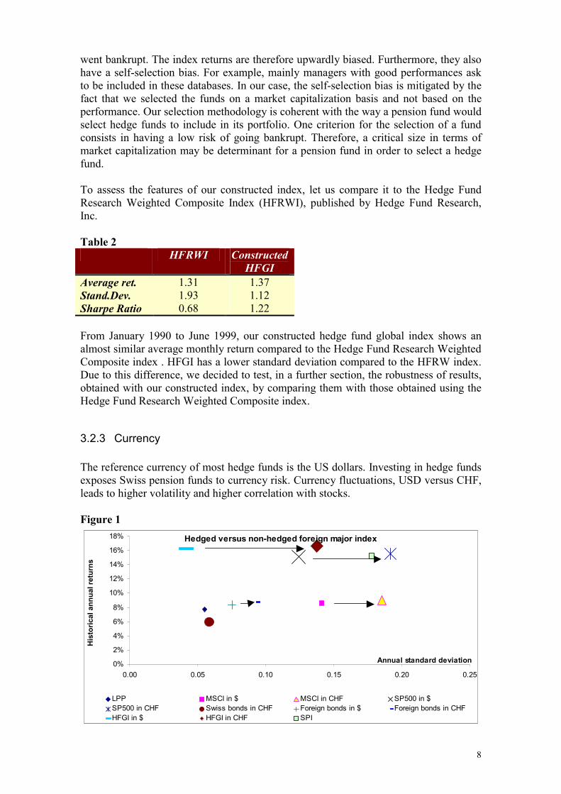
3.2.3 Currency The reference currency of most hedge funds is the US dollars. Investing in hedge funds exposes Swiss pension funds to currency risk. Currency fluctuations, USD versus CHF, leads to higher volatility and higher correlation with stocks. Figure 1
Hedged versus non-hedged foreign major index
0%
2%
4%
6%
8%
10%
12%
14%
16%
18%
0.00 0.05 0.10 0.15 0.20 0.25
Annual standard deviation
His
toric
al a
nnua
l ret
urns
LPP MSCI in $ MSCI in CHF SP500 in $SP500 in CHF Swiss bonds in CHF Foreign bonds in $ Foreign bonds in CHFHFGI in $ HFGI in CHF SPI
9
Figure 1 shows the impact of the exchange rate on the volatility for different indices over a period of ten years, that is from January 1989 to June 1999. One should remember that the Swiss franc variance of a foreign investment is equal to its variance in the local currency plus the variance of the exchange rate plus twice the covariance between the investment return and the exchange rate movement. This figure confirms that currency risk increases the volatility of the foreign investments and that it may have a significant impact on hedge funds investments. Nevertheless, the objective of an optimal investment policy is not to minimize risk but to optimize the risk-adjusted performance. A systematic policy of complete currency hedging would eliminate the contribution of currency risk to the total volatility of the portfolio. Furthermore, in the case of hedge fund investments, it allows to maintain important features of hedge funds like a low volatility and low correlation. But hedging has a cost and a systematic full hedging may turn out to be costly. Therefore, the hedging policy should depend on the investor's objectives. It is not in the scope of this master's thesis to analyze currency risk in detail. In order to focus only on hedge fund characteristics and their implications on portfolio asset allocation, we will assume that Swiss pension funds are able to fully and perfectly hedge their foreign investments.
3.3 Mean-variance analysis
3.3.1 Efficient frontier analysis In recent years, a lot of press releases were published on the industry of hedge funds. Some articles mention the advantages of these financial instruments and others highlight theirs dangers. This was particularly true after the near debacle of the LTCM fund or the impressive returns obtained by some Macro funds. "Put your money in hedge funds: it's safer", this is what one of the biggest banks in the world told to its U.S. pension fund clients in a booklet published in July 1998. One way to analyze the benefits for a Swiss Pension Fund to invest in hedge funds in a mean-variance setting, consists in looking at the impact of the decision on the efficient frontier. One can assert that an asset or a portfolio X dominates an asset or a portfolio Y if the expected return X is greater than the expected return of Y and if simultaneously the variance of X is lower or equal to the variance of Y. Thus, the efficient frontier can be defined as the locus of all non-dominated portfolios in the mean-variance space. By definition, no mean-variance investor would choose to hold a portfolio not located on the efficient frontier. The shape of the efficient frontier is thus of primary interest. The available set of assets is composed of stocks, bonds and hedge funds. They are represented by the following indices mentioned above, that is the Swiss Performance Index (SPI), the MSCI index, the Salomon Brother Weighted Global Bond index (SBWBI), the Salomon Brother Weighted Swiss Bond Index (SBSBI) and the Hedge Fund Equally Weighted Global Index (HFGI). The analysis is performed over a period of about 10 years, from January 1989 to July 1999 inclusive. We obtain the optimal portfolios by minimizing the portfolio variance for a given rate of return. With the set of optimal portfolios, it is then possible to draw the efficient frontier. We first assume that hedge funds are not available for investment purposes. We assume, then, that Swiss pension funds can invest part of their wealth in them. The analysis cannot be done without taking into account the legal requirements of the LPP in terms of investment limits. We, therefore, include some constraints in our
10
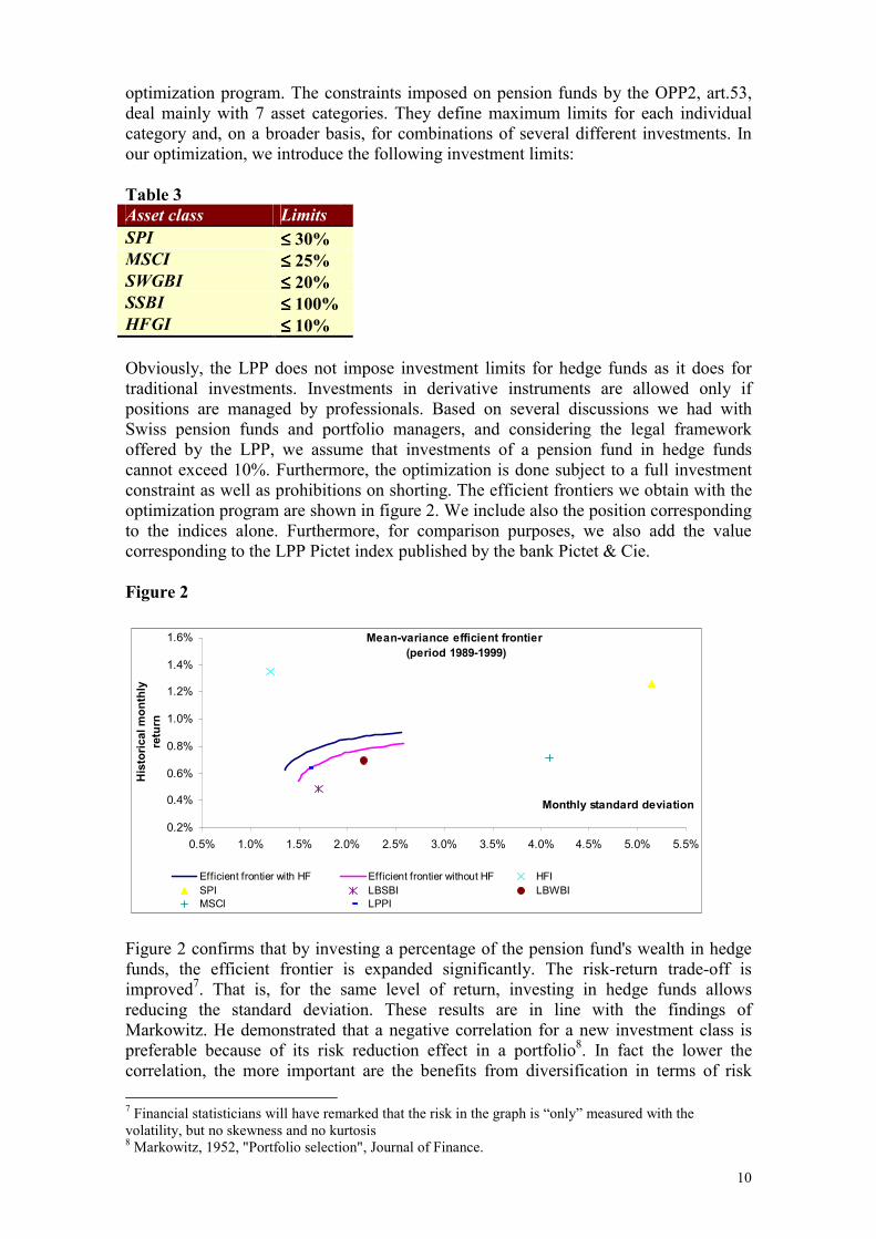
optimization program. The constraints imposed on pension funds by the OPP2, art.53, deal mainly with 7 asset categories. They define maximum limits for each individual category and, on a broader basis, for combinations of several different investments. In our optimization, we introduce the following investment limits: Table 3 Asset class Limits SPI ≤≤≤≤ 30% MSCI ≤≤≤≤ 25% SWGBI ≤≤≤≤ 20% SSBI ≤≤≤≤ 100% HFGI ≤≤≤≤ 10% Obviously, the LPP does not impose investment limits for hedge funds as it does for traditional investments. Investments in derivative instruments are allowed only if positions are managed by professionals. Based on several discussions we had with Swiss pension funds and portfolio managers, and considering the legal framework offered by the LPP, we assume that investments of a pension fund in hedge funds cannot exceed 10%. Furthermore, the optimization is done subject to a full investment constraint as well as prohibitions on shorting. The efficient frontiers we obtain with the optimization program are shown in figure 2. We include also the position corresponding to the indices alone. Furthermore, for comparison purposes, we also add the value corresponding to the LPP Pictet index published by the bank Pictet & Cie. Figure 2
Figure 2 confirms that by investing a percentage of the pension fund's wealth in hedge funds, the efficient frontier is expanded significantly. The risk-return trade-off is improved7. That is, for the same level of return, investing in hedge funds allows reducing the standard deviation. These results are in line with the findings of Markowitz. He demonstrated that a negative correlation for a new investment class is preferable because of its risk reduction effect in a portfolio8. In fact the lower the correlation, the more important are the benefits from diversification in terms of risk 7 Financial statisticians will have remarked that the risk in the graph is “only” measured with the volatility, but no skewness and no kurtosis 8 Markowitz, 1952, "Portfolio selection", Journal of Finance.
Efficient frontier with HF Efficient frontier without HF HFISPI LBSBI LBWBIMSCI LPPI
11
reduction and return enhancement. Figure 2 confirms the benefits from the diversification. All single indices are outperformed by the efficient frontiers, except for the LPP Pictet index and the hedge fund index. This is logical for the LPP index as it is composed of the same asset classes as the optimal portfolios, which form the efficient frontier obtained without hedge funds available for investment. This is confirmed by the statistics based on monthly data provided in table 4. Table 4 Asset class Exp. Ret. Stand.Dev. Sharpe Ratio SPI 1.25% 5.14% 0.246 MSCI 0.71% 4.08% 0.175 LBSBI 0.48% 1.70% 0.285 LBWBI 0.70% 2.17% 0.321 HFGI 1.35% 1.20% 1.124 LPPI 0.64% 1.60% 0.402 Note that we assume a risk free interest rate equal to zero. The hedge fund index clearly outperforms the other indices on a Sharpe ratio basis. This is in line with various papers published on the subject. Edwards and Liew (1999)9 and Cottier (1997)10 conclude that Hedge Funds as a stand-alone investments outperform stocks and bonds on a return and a risk-return basis. The high risk-adjusted returns earned by hedge funds raise the issue of understanding the source of this performance. Are these funds capturing market inefficiencies, do hedge fund portfolio managers possess higher trading skills or is the investor simply paying for taking specific risks which appear to a lesser extend with standard investment classes such as stocks and bonds? These questions are of major concern and will be subject to a closer analysis later in our paper.
3.3.2 Correlation analysis An interesting information concerns the degree of linear correlation of the hedge fund index with other indices. Table 5 Correlation MSCI SPI SBWBI SBSBI HFGI
MSCI 1 0.68 0.33 0.10 0.35 SPI 1 -0.08 0.27 0.43
SBWBI 1 0.25 -0.07 SBSBI 1 0.06 HFGI 1
The hedge fund global index shows a lower linear correlation level with bond indices and is slightly higher with stock indices11. This is an important result considering that Swiss pension funds invest highly in bonds. Again this result is in line with those obtained in previous studies.
9 Franklin R. Edwards and Jimmy Liew, 1999, Hedge Funds versus Managed Futures As Asset Classes, The Journal of Derivatives. 10 Philipp Cottier, 1997, Hedge Funds and Managed Futures: Performance, Risks, Strategies and Use in Investment Portfolios, Haupt. 11 Financial statisticians will have remarked that a linear correlation underestimates the true relation when the relation between the 2 assets is non linear
12
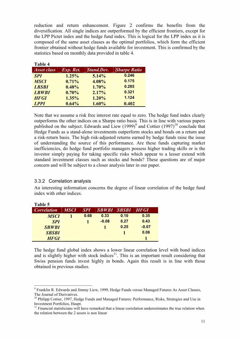
Hedge funds are largely unregulated. Usually, they have flexible investment strategies and are allowed to use leverage, derivative products and take short positions. These characteristics allow hedge funds to exhibit low correlation coefficients with traditional financial products. This has been confirmed by empirical studies published over the last years. The correlation obtained in table 5 is obviously an interesting characteristic as it suggests that hedge funds may provide diversification for portfolio investors. Nevertheless, this diversification benefit is valuable as long as the correlation is stable over time. Furthermore, the underlying assumption of the traditional correlation coefficient is that there is a linear relationship between the two financial instruments analyzed. Due to the characteristics of hedge funds, the linear relationship assumption may be too restrictive. Therefore, another way to analyze the correlation should be implemented. Let us take the case of the LPP Pictet index and our hedge fund global index. The linear correlation coefficient between both indices is given by12
Based on this formula, the correlation between the hedge fund index and the LPP Pictet index over the period from January 1989 to June 1989, equals 0.44. Figure 3 analyzes the returns of the HFGI compared to the returns of the LPP Pictet Index over the same period of time. The LPP Pictet Index measures a theoretical average performance of portfolios subject to the legal requirements in terms of investment constraints (see table 3). Figure 3
Source: authors, Altvest database, datastream There is a positive correlation for positive LPP returns and another one for negative LPP returns:
12 In a mean-variance setting, the risk is measured with the variance of the portfolio and is equal to σ2(portfolio)= w2
LPPσ2LPP+w2
HFGIσ2HFGI + 2 wLPP wHFGI cov(rLPP;rHFGI)
HFGiLPP *)HFGI,LPPcov(
σσ=ρ
ρσ σ+
++= =cov( ; ) .LPP HFGILPP HFGI
0 47 ρσ σ−
−−= =cov( ; ) .LPP HFGILPP HFGI
0 07
LPP Pictet Index vs Hedge Funds Global Index
-6%
-4%
-2%
0%
2%
4%
6%
His
toric
al m
onth
yl re
turn
s
Return HF Global IndexReturn LPP
13
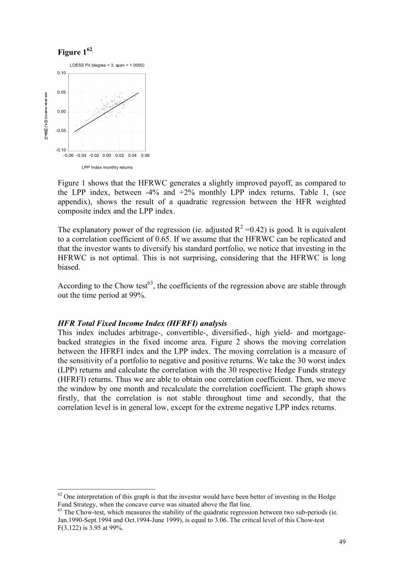
It seems, therefore, that the coefficient of correlation is not stable over time and that the assumption of linear relationship is not verified. These characteristics can be highlighted with a local regression analysis. Figure 4 shows this idea: Figure 4 The straight line represents the payoff of a 100% investment in the LPP Pictet index. The "concave" line is the result of the local regression analysis obtained with the Loess Fit technique13. First we observe that the relationship between both indices is far from being linear. We can also see that investing in the hedge fund global index is profitable when returns of the LPP index are below 2%. The "concave" shape suggests that an investor who buys this hedge fund global index is selling options. Therefore, the vision of the investor buying our constructed diversified Hedge Funds index is bearish in the volatility, stable or bearish on the market.
3.4 Out-of-sample portfolio performance analysis in a mean-variance framework
One step further in our methodology involves analyzing the out-of-sample performance of the optimized portfolios. We split our sample in two. Data from January 1989 to December 1994 is used to get the optimal weights for each asset class. From January 1995 to June 1999, the performance of the optimal portfolio with hedge funds is then compared with the optimal portfolio without hedge funds. We take three different examples for which we assume different constraints and investment objectives.
3.4.1 Example 1 First, we assume that the investment objective of the Swiss pension fund consists in maximizing the Sharpe ratio. We assume that cash invested without risk does not pay any return. The risk free rate of return, therefore, equals zero. We maximize the Sharpe ratio so that no short selling is allowed, a full investment is required and the investment constraints in table 2 are satisfied.
13 For more information on local regression analysis, see Chambers, Hastie, Statistical models in S, 1992, chapter 8, Wadsworth & Brooks.
-0.04
-0.02
0.00
0.02
0.04
0.06
-0.06 -0.04 -0.02 0.00 0.02 0.04 0.06
LPP monthly returns
HFGI monthly returns
LOESS Fit (degree = 2, span = 0.8000)
14
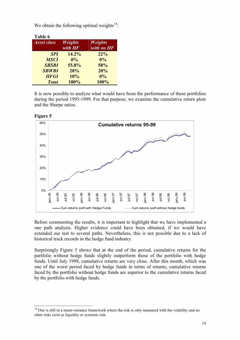
We obtain the following optimal weights14: Table 6 Asset class Weights
with HF Weights with no HF
SPI 14.2% 22% MSCI 0% 0%
SBSBI 55.8% 58% SBWBI 20% 20%
HFGI 10% 0% Total 100% 100%
It is now possible to analyze what would have been the performance of these portfolios during the period 1995-1999. For that purpose, we examine the cumulative return plots and the Sharpe ratios. Figure 5
Before commenting the results, it is important to highlight that we have implemented a one path analysis. Higher evidence could have been obtained, if we would have extended our test to several paths. Nevertheless, this is not possible due to a lack of historical track records in the hedge fund industry. Surprisingly Figure 5 shows that at the end of the period, cumulative returns for the portfolio without hedge funds slightly outperform those of the portfolio with hedge funds. Until July 1998, cumulative returns are very close. After this month, which was one of the worst period faced by hedge funds in terms of returns, cumulative returns faced by the portfolio without hedge funds are superior to the cumulative returns faced by the portfolio with hedge funds. 14 One is still in a mean-variance framework where the risk is only measured with the volatility and no other risks exist as liquidity or systemic risk.
Standard Deviation 1.23% 1.57% Sharpe ratio 0.722 0.577%
Table 7 confirms that the traditional portfolio outperforms the portfolio with hedge funds on a return basis. Nevertheless, on a risk-adjusted basis the portfolio with hedge funds is clearly better. The main observation that we can draw from these results is that the inclusion of 10% of hedge funds in the traditional portfolio has an important diversification effect. The volatility of the traditional portfolio decreases, which improves the Sharpe ratio.
3.4.2 Example 2 Let us now assume that the investor still has the same objective, that is to maximize the Sharpe ratio without any constraints regarding the investment limits by asset class. Thus, we will compute the optimal portfolio in a mean-variance framework. Therefore, total investment in hedge funds is no more limited to 10% of the wealth. Full investment constraint and no short selling assumption are kept. We obtain the following weights: Table 8 Asset class Weights
with HF Weights
without HF SPI 0% 15.1%
MSCI 0% 0% SBSBI 0% 11.3/
SBWBI 11% 73.6% HFGI 89% 0% Total 100% 100%
Based on the optimization without limit constraints, we should invest 89% of the total wealth in hedge funds. This is not really a surprise considering the level of the risk-adjusted return of our constructed hedge fund index. Over the period between January 1995 to June 1999, the cumulative returns are the following: Figure 6
Cumulative returns (period 1995-1999) No constraints
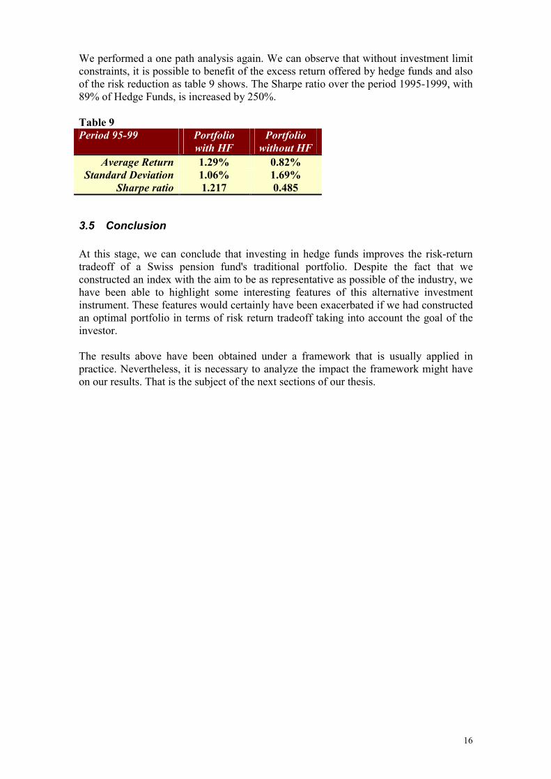
We performed a one path analysis again. We can observe that without investment limit constraints, it is possible to benefit of the excess return offered by hedge funds and also of the risk reduction as table 9 shows. The Sharpe ratio over the period 1995-1999, with 89% of Hedge Funds, is increased by 250%. Table 9 Period 95-99 Portfolio
with HF Portfolio
without HF Average Return 1.29% 0.82%
Standard Deviation 1.06% 1.69% Sharpe ratio 1.217 0.485
3.5 Conclusion At this stage, we can conclude that investing in hedge funds improves the risk-return tradeoff of a Swiss pension fund's traditional portfolio. Despite the fact that we constructed an index with the aim to be as representative as possible of the industry, we have been able to highlight some interesting features of this alternative investment instrument. These features would certainly have been exacerbated if we had constructed an optimal portfolio in terms of risk return tradeoff taking into account the goal of the investor. The results above have been obtained under a framework that is usually applied in practice. Nevertheless, it is necessary to analyze the impact the framework might have on our results. That is the subject of the next sections of our thesis.
17
4 Assumptions underlying the mean-variance theory
4.1 Introduction Financial theory has devoted a lot of time and resources to understand the determinants of the demand for different securities. This is directly linked with the theory of choice made by a rational agent in a situation of uncertainty. This reflection on the demand of agents requires the understanding of how financial risk is measured and how an investor's attitude towards risk is to be conceptualized and measured. The objective of this section consists in explaining and, then, testing the different assumptions underlying the use of the mean-variance theory for asset allocation with alternative investments.
4.1.1 Mean-variance criterion for investment selection In finance, risk is typically defined as the uncertainty of future cash-flow streams of an asset. Let us take the following example: Asset payoffs t=0 t=1 State of nature 1
(probability:1/2) State of nature 2 (probability:1/2)
Investment 1 -100 80 150 Investment 2 -100 40 180
or in term of returns t=1 State of nature 1 State of nature 2Investment 1 -20% +50% Investment 2 -60% +80%
Both investments have an initial cost of 100. One period later, in t=1, they have different payoffs depending on the state of nature. The probability of each state is equal. In our case asset 2 seems to be riskier than asset 1 but with a greater potential of return. Therefore, it is difficult to say which of them dominates the other one. The ranking between these two investments is preference dependent. The theory of choice under uncertainty has developed several types of criteria in order to modelize how a rational agent is going to make his choice. These criteria are, for example, the maximin of Wald or the criterion of Hurwicz. Nevertheless, it is customary to summarize this investment return distribution by the mean and the variance. In this case, the variance or the standard deviation is used as a measure of risk. Mean Variance Investment 1 15% 24.5% Investment 2 10% 98%
Considering the mean and the variance, asset 1 dominates asset 2. It has a greater mean with a lower variance. The mean-variance criterion says that for investments of the
18
same expected rate of return, choose the one with the lowest variance and for investments of the same variance, choose the one with the greatest expected return. This criterion is the simplest to understand as it uses only the first two moments of the asset returns distribution. The difficulty in applying it in practice lies in the fact that we don't know the probabilities of the states of nature ex-ante. That is, we don't know ex-ante the returns' distribution. A frequently used proxy for a future return distribution is its historical one. For example, we can decide to select the last monthly returns over a period of 5 years. The mean and variance of these 60 monthly returns are then used as a proxy of the future mean and variance of the returns. By doing that we assign a probability of 1/60 to each past observation. Firstly, we assume that the return realizations are independent of each other and secondly that the returns of the asset are stationary. In other words, we assume that the future is going to repeat itself.
4.2 Assumptions underlying the mean-variance portfolio theory The concept of utility function allows taking into account the preferences and the risk aversion of the investors. This is obviously an important advantage compared to the simple mean-variance criterion. Nevertheless, the most part of financial institutions still use the last criterion as a consequence of the findings of the Modern Portfolio Theory. This theory has been developed using the concept of utility functions. But by postulating either that the utility function of the investor is quadratic or that the investor's end of period wealth is normally distributed, it is possible to justify the choice of the mean-variance criteria. At this stage, it may be important to observe that our goal is not to explain the concepts underlying the Modern Portfolio Theory. Our objective is to highlight the fact that there are strong assumptions behind the mean-variance framework. When a new financial product is available, like hedge funds, it is interesting to analyze if these assumptions are still valid and, if not, to understand the consequences and the limitations of the theory.
4.2.1 Quadratic utility function The first way to justify the use of the mean-variance theory is to assume that investors have a quadratic utility function:
Taking this utility function, it can be demonstrated that mean-variance decision making process leads to optimal choices. Nevertheless, the quadratic utility function has some properties that are hardly satisfied.
2)( bWaWWU −=
19
Pratt (1964) and Arrow(1971) have developed two widely used measures of risk aversion: Absolute risk aversion: Relative risk aversion:
The absolute risk aversion measures the risk aversion for a given level of wealth. This definition of risk aversion is useful because it provides an interesting insight of people's behavior in the face of risk. Empirically we know that absolute risk aversion will probably decrease as wealth increases. If we multiply the value of absolute risk aversion by the level of wealth, we obtain the relative risk aversion. Constant relative risk aversion implies that an individual will have constant risk aversion to a proportional loss of wealth even though the absolute loss increases at the same time as wealth does. If we take the case of the quadratic utility function, the absolute risk aversion is given by:
If we analyze the behavior of the risk aversion as a function of the wealth, we observe that the absolute risk aversion is an increasing function of wealth:
Obviously, this result is not fully satisfactory as it does not correspond to the rational behavior of an investor. It is, therefore, difficult to justify the use of the mean-variance theory with the assumption about agents' preferences.
4.2.2 Normally distributed returns The second assumption that can be done to justify the use of the modern portfolio theory is the normality of the returns' distribution. The normal distribution has the property that it can be completely described by two parameters: its mean and variance. This is a bell-shaped probability distribution that many natural phenomena obey to. When a phenomenon is subject to numerous influences independent of each other, the values of this phenomenon are distributed according to the normal distribution. The normal distribution is perfectly symmetric, 50% of the probability lies above the mean. Therefore, the skewness and the kurtosis, which are, respectively, the third and fourth moment of the distribution, are equal to 0 and 3. The following chart represents a standard normal distribution curve. It has been randomly generated with a statistical software. The standard normal distribution is characterized by the fact that its mean and standard deviation are respectively equal to 0 and 1.
)()()(
WUWUWAR
′′′
−=)(
)(*)(WU
WUWWRR′′′
−=
bWabWAR2
2)(−
=
0)2(
4)(2
2
bWab
WWAR
−=
∂∂
20
If the mean and the standard deviation of the normal distribution are known, then the likelihood of every point in the distribution is also known. This would not be true if the distribution was not symmetric. The probability to lie within the limits of µ ± σ is 68.27% and within the limits of µ ± 2σ is 95.45%. In the case of a skewness, for example, which were not equal to 0, the mean and the variance would not be enough to know the probability to lie within a range of values. Therefore, the analysis of the returns' true distribution is important for proper risk management and portfolio allocation.
4.2.3 Hedge Fund Global Index analysis Our Hedge Fund Global Index is composed of 53 hedge funds. They have been selected among the different investment strategies available. As discussed previously, some of the defining characteristics of hedge funds are the regular use of short positions, leverage and derivatives instruments in their investment strategy. It is interesting to analyze the distribution of our hedge fund index and to see how these features may affect it. We obtain the distribution based on monthly returns from January 1989 to June 1999. We observe that the returns' distribution of our hedge fund index has not the same bell shape. First, the skewness is negative. This suggests that the distribution is not symmetric. The probability to have returns which are lower than the mean is higher than 50%. Then, the kurtosis is much higher than 3. This distribution has fat tails. Obviously, these findings may have important impacts on the risk assessment of the global investment portfolio.
0
200
400
600
800
1000
1200
-3 -2 -1 0 1 2 3 4
Series: DISTRSample 1 10000Observations 10000
Mean -0.005770Median -0.004278Maximum 4.255807Minimum -3.744810Std. Dev. 0.994403Skewness 0.007913Kurtosis 3.018883
Jarque-Bera 0.252937Probability 0.881202
0
5
10
15
20
25
-0.025 0.000 0.025
Series: HFSample 1989:01 1999:06Observations 126
Mean 0.013537Median 0.015726Maximum 0.043883Minimum -0.037080Std. Dev. 0.012040Skewness -1.379540Kurtosis 7.423158
Jarque-Bera 142.6785Probability 0.000000
21
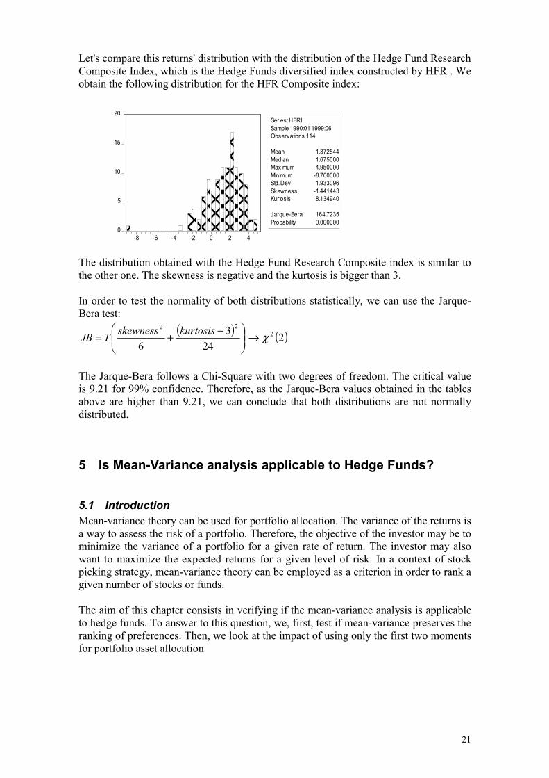
Let's compare this returns' distribution with the distribution of the Hedge Fund Research Composite Index, which is the Hedge Funds diversified index constructed by HFR . We obtain the following distribution for the HFR Composite index: The distribution obtained with the Hedge Fund Research Composite index is similar to the other one. The skewness is negative and the kurtosis is bigger than 3. In order to test the normality of both distributions statistically, we can use the Jarque-Bera test:
( ) ( )224
36
222
χ→
−+= kurtosisskewnessTJB
The Jarque-Bera follows a Chi-Square with two degrees of freedom. The critical value is 9.21 for 99% confidence. Therefore, as the Jarque-Bera values obtained in the tables above are higher than 9.21, we can conclude that both distributions are not normally distributed.
5 Is Mean-Variance analysis applicable to Hedge Funds?
5.1 Introduction Mean-variance theory can be used for portfolio allocation. The variance of the returns is a way to assess the risk of a portfolio. Therefore, the objective of the investor may be to minimize the variance of a portfolio for a given rate of return. The investor may also want to maximize the expected returns for a given level of risk. In a context of stock picking strategy, mean-variance theory can be employed as a criterion in order to rank a given number of stocks or funds. The aim of this chapter consists in verifying if the mean-variance analysis is applicable to hedge funds. To answer to this question, we, first, test if mean-variance preserves the ranking of preferences. Then, we look at the impact of using only the first two moments for portfolio asset allocation
Mean 1.372544Median 1.675000Maximum 4.950000Minimum -8.700000Std. Dev. 1.933096Skewness -1.441443Kurtosis 8.134940
Jarque-Bera 164.7235Probability 0.000000
22
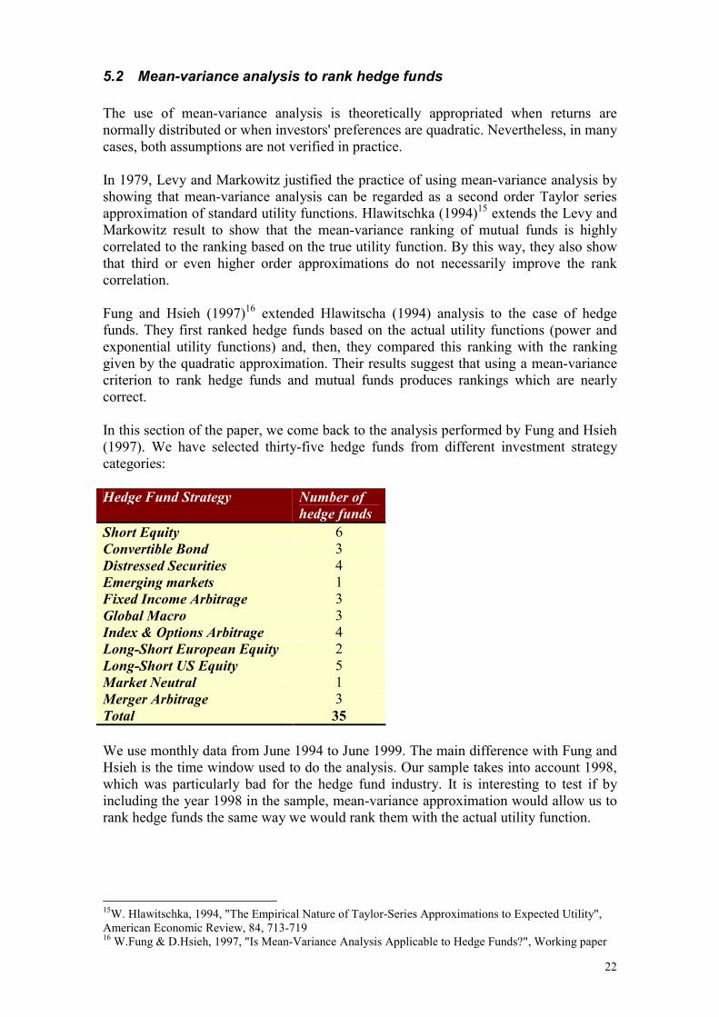
5.2 Mean-variance analysis to rank hedge funds The use of mean-variance analysis is theoretically appropriated when returns are normally distributed or when investors' preferences are quadratic. Nevertheless, in many cases, both assumptions are not verified in practice. In 1979, Levy and Markowitz justified the practice of using mean-variance analysis by showing that mean-variance analysis can be regarded as a second order Taylor series approximation of standard utility functions. Hlawitschka (1994)15 extends the Levy and Markowitz result to show that the mean-variance ranking of mutual funds is highly correlated to the ranking based on the true utility function. By this way, they also show that third or even higher order approximations do not necessarily improve the rank correlation. Fung and Hsieh (1997)16 extended Hlawitscha (1994) analysis to the case of hedge funds. They first ranked hedge funds based on the actual utility functions (power and exponential utility functions) and, then, they compared this ranking with the ranking given by the quadratic approximation. Their results suggest that using a mean-variance criterion to rank hedge funds and mutual funds produces rankings which are nearly correct. In this section of the paper, we come back to the analysis performed by Fung and Hsieh (1997). We have selected thirty-five hedge funds from different investment strategy categories: Hedge Fund Strategy Number of
hedge funds Short Equity 6 Convertible Bond 3 Distressed Securities 4 Emerging markets 1 Fixed Income Arbitrage 3 Global Macro 3 Index & Options Arbitrage 4 Long-Short European Equity 2 Long-Short US Equity 5 Market Neutral 1 Merger Arbitrage 3 Total 35 We use monthly data from June 1994 to June 1999. The main difference with Fung and Hsieh is the time window used to do the analysis. Our sample takes into account 1998, which was particularly bad for the hedge fund industry. It is interesting to test if by including the year 1998 in the sample, mean-variance approximation would allow us to rank hedge funds the same way we would rank them with the actual utility function.
15W. Hlawitschka, 1994, "The Empirical Nature of Taylor-Series Approximations to Expected Utility", American Economic Review, 84, 713-719 16 W.Fung & D.Hsieh, 1997, "Is Mean-Variance Analysis Applicable to Hedge Funds?", Working paper
23
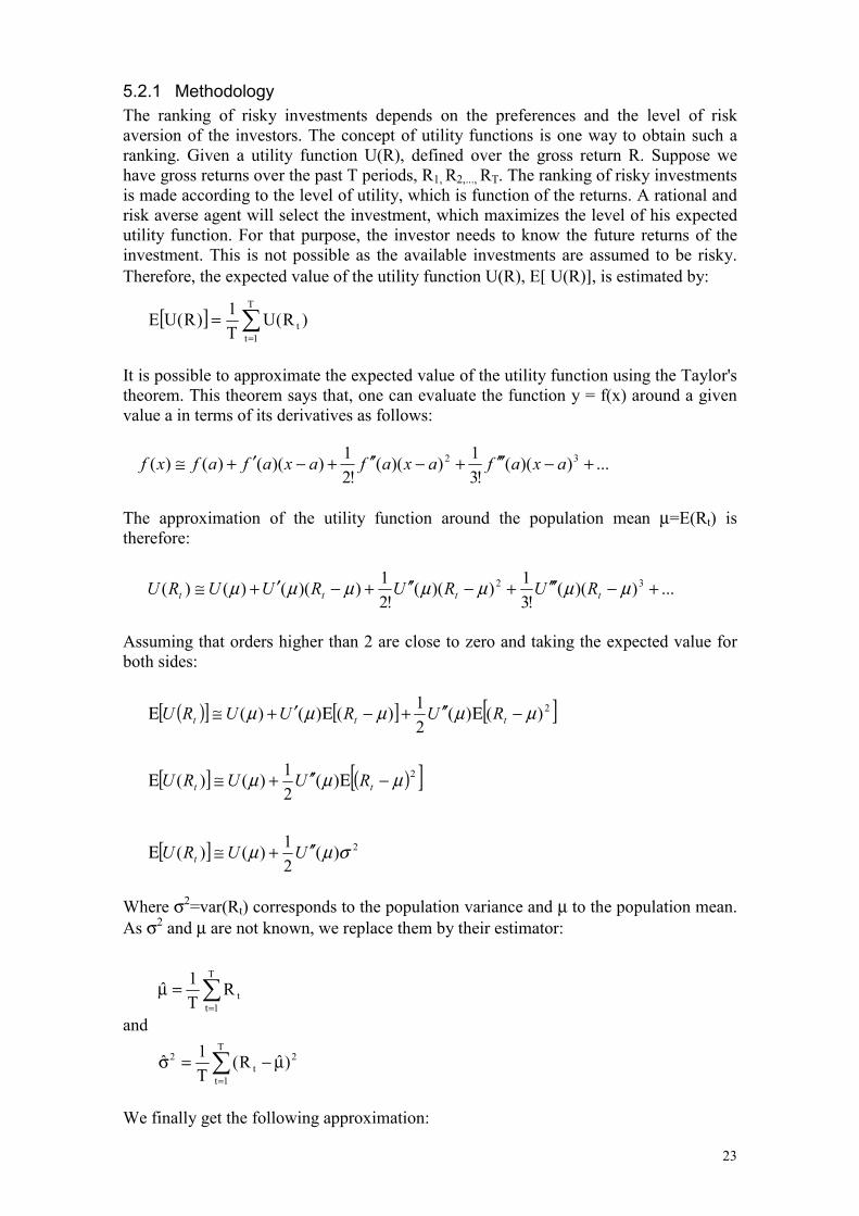
5.2.1 Methodology The ranking of risky investments depends on the preferences and the level of risk aversion of the investors. The concept of utility functions is one way to obtain such a ranking. Given a utility function U(R), defined over the gross return R. Suppose we have gross returns over the past T periods, R1, R2,..., RT. The ranking of risky investments is made according to the level of utility, which is function of the returns. A rational and risk averse agent will select the investment, which maximizes the level of his expected utility function. For that purpose, the investor needs to know the future returns of the investment. This is not possible as the available investments are assumed to be risky. Therefore, the expected value of the utility function U(R), E[ U(R)], is estimated by:
It is possible to approximate the expected value of the utility function using the Taylor's theorem. This theorem says that, one can evaluate the function y = f(x) around a given value a in terms of its derivatives as follows:
The approximation of the utility function around the population mean µ=E(Rt) is therefore:
Assuming that orders higher than 2 are close to zero and taking the expected value for both sides:
Where σ2=var(Rt) corresponds to the population variance and µ to the population mean. As σ2 and µ are not known, we replace them by their estimator:
The expected value of the utility function is approximated with the sample mean and the sample variance. To assess the quality of this approximation, we select two widely used utility functions. Like Fung and Hsieh (1997), we assume that investors have either power utility function or exponential utility function. Power utility function:
where γ is the Arrow-Pratt coefficient of risk aversion and W the level of wealth after one period return. We assume that the initial level of wealth W0 = 100. Exponential Utility function:
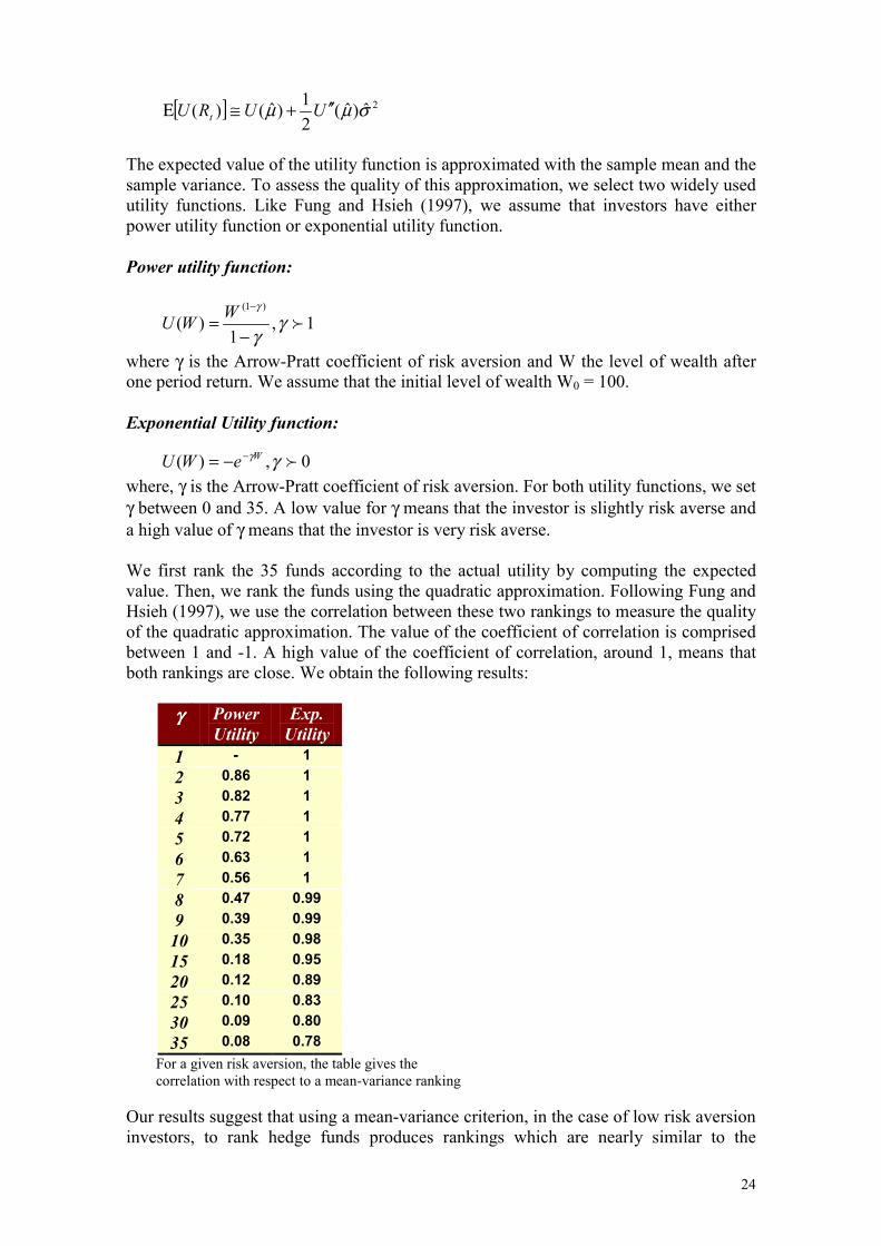
where, γ is the Arrow-Pratt coefficient of risk aversion. For both utility functions, we set γ between 0 and 35. A low value for γ means that the investor is slightly risk averse and a high value of γ means that the investor is very risk averse. We first rank the 35 funds according to the actual utility by computing the expected value. Then, we rank the funds using the quadratic approximation. Following Fung and Hsieh (1997), we use the correlation between these two rankings to measure the quality of the quadratic approximation. The value of the coefficient of correlation is comprised between 1 and -1. A high value of the coefficient of correlation, around 1, means that both rankings are close. We obtain the following results:
For a given risk aversion, the table gives the correlation with respect to a mean-variance ranking Our results suggest that using a mean-variance criterion, in the case of low risk aversion investors, to rank hedge funds produces rankings which are nearly similar to the
[ ] 2ˆ)ˆ(21)ˆ()( σµµ UURU t ′′+≅Ε
1,1
)()1(
γγ
γ
−=
−WWU
0,)( γγWeWU −−=
25
rankings obtained with the actual utility functions. Nevertheless, the quality of the approximation decreases with the increase of the agent's risk aversion. In general, the exponential utility function produces better results. With a degree of risk aversion of 35, we still have a ranking correlation of 0.78. In contrast, the coefficient of correlation is lower with the power utility function. Moreover, it deteriorates a lot with high degrees of risk aversion. Thus, this criterion seems to work poorly with agents having high degrees of risk aversion. These results are significantly different from those obtained by Fung & Hsieh in 1997. Their results show that using mean-variance criterion to rank hedge funds produces rankings close to those obtained with the actual utility function. That is, the coefficient of correlation is close to 1 even when we use high degrees of risk aversion. This difference in the results may be due to the time window used to do the analysis. As previously mentioned, we take into account 1998 which was a poor performing year for the hedge fund industry. To understand the reason of this difference between both function utilities, we performed the same test with a three months interval, that is we used quarterly data from June 1994 to June 1999. With quarterly data, the correlation with the exponential utility function do not significantly change. The opposite is true for the power utility function, which correlation coefficients increase significantly (max correlation coef.=0.99 and minimum=0.4). Thus, we can conclude that the power utility function is more sensitive than the exponential to the sample data used and its fluctuations. By taking quarterly data, price's fluctuations (volatility) are reduced. Finally, we test the appropriateness of using the Sharpe ratio. This criteria assumes that each agent, willing to invest in risky assets, makes his decisions based on mean-variance criterion and that he attributes the same tradeoff between risk and return. This tradeoff is represented by the ratio E(R)/σ. We do not use the traditional Sharpe ratio as we don't subtract the risk free rate from the numerator. We first rank the hedge funds based on the Sharpe ratio and then, we compare it with the ranking obtained with the actual utility function. Again, both rankings are compared using the coefficient of correlation. We obtain the following results:
For a given risk aversion, the table gives the correlation with respect to a mean-variance ranking
26
It is interesting to observe that using the Sharpe ratio to rank hedge funds produces rankings which are nearly correct when the degree of risk aversion is high, in the case of the exponential utility function. The results obtained with the power utility function are far from 1, whatever the degree of risk aversion is. Fung and Hsieh (1997) also find that this criterion works poorly when the risk aversion is low but they suggest that it works reasonably well when the risk aversion is high. Furthermore, the different results obtained with one utility function and the other one are, again, due to the sensitivity of the power utility function to return fluctuation.. If we take only quarterly data, we observe that correlation coefficients obtained with the power utility are significantly improved.
5.2.2 Conclusion Our results show that the effectiveness of the criterion that an investor chooses in order to rank hedge funds strongly depends on his degree of risk aversion. We show that an investor with a low risk aversion should use the quadratic approximation criterion and therefore the mean variance theory. In the case of a highly risk averse investor, like a pension fund for example, he should use the Sharpe ratio. More generally, we have shown that criteria defined only over the mean and variance of the returns' distribution are not fully satisfactory. The quality of the results depends on the degree of risk aversion and on the type of utility function. Our results clearly differ from those obtained by Fung & Hsieh (1997). The reason for this difference can be found in the time window used to do the analysis. As already said, we took hedge funds' returns between 1994 and 1999. Therefore, we included the year 1998, which was a bad year for hedge funds. Thus, this difference in methodology and its impact on the results suggest that the appropriateness of using a mean-variance criterion mainly depends on the degree of non-normality of the returns.
5.3 Mean –modified Value-at-Risk optimization
5.3.1 Introduction We have seen that the use of the mean-variance approach to rank funds has some drawbacks. As a consequence, we decided to look at the benefits of investing in hedge funds using another framework, that is using mean-Value-at-Risk setting. Until now, risk was measured by the volatility of the returns. Nevertheless, other approaches are available to measure the risk of a portfolio. The most traditional is the Value at Risk, which integrates the notion of downside risk. The downside risk is incorporated into the asset allocation model. The optimal portfolio is selected by maximizing the expected return over candidate portfolios so that some shortfall criterion is met. The literature expanded a lot on the Value at Risk subject these recent years. Uryasev and Rockafellar (1999)17 propose to measure a Mean Shortfall or Conditional VaR which is the mean of the returns higher than the VaR. Flavin and Wickens (1998)18 use a Garch process to model asset returns. Artzner, Delbaen, Eber and Heath (1997)19 argue that their 17 Uryasev, Rockafellar, 1999, Optimization of conditional VaR, University of Florida, Working paper. 18 Flavin, Wickens, 1998, A risk management approach to optimal asset allocation, University of New-York, Working paper. 19 Artzner, Delbaen, Eber, Heath, 1997, Coherent measures of risk, Carnegie Mellon University, Working paper.
27
proposed coherent measures of risks have certain desirable properties that VaR lacks of. Basak and Shapiro (1998)20 argue that VaR does not consider the magnitude of loss, which exceeds the threshold level. They propose an analytical formula to obtain the portfolio's weights of risky assets, assuming that they are log-normally distributed, by minimizing the losses over a threshold. In this section, we first introduce the framework. It is based on the working paper by Huisman, Koedijk and Pownall (1999)21. Then, we show some empirical results and highlight the importance of non-normal characteristics of some returns' distributions. Finally, we compute the optimal weights in a mean-VaR setting taking into account these non-normal features.
5.3.2 Asset allocation in a mean-modified Value-at-Risk framework Introduction The risk of a portfolio composed of financial assets can be measured with the VaR. The VaR, as a measure of risk, has some interesting advantages: • It is recognized by practitioners, • It is easy to understand and to implement, • It measures the downside risk which is interesting for a risk averse investor like a
pension fund, • Many academic studies have been done on the subject, • We can measure risk with just one easily understandable number. • It can be used for non-normally distributed assets. We will adjust the Value-at-Risk
method by using an empirical VaR and an analytical VaR, which takes the skewness and the kurtosis into account.
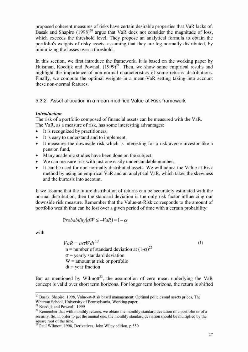
If we assume that the future distribution of returns can be accurately estimated with the normal distribution, then the standard deviation is the only risk factor influencing our downside risk measure. Remember that the Value-at-Risk corresponds to the amount of portfolio wealth that can be lost over a given period of time with a certain probability:
with
n = number of standard deviation at (1-α)22 σ = yearly standard deviation W = amount at risk or portfolio dt = year fraction But as mentioned by Wilmott23, the assumption of zero mean underlying the VaR concept is valid over short term horizons. For longer term horizons, the return is shifted 20 Basak, Shapiro, 1998, Value-at-Risk based management: Optimal policies and assets prices, The Wharton School, University of Pennsylvania, Working paper. 21 Koedijk and Pownall, 1999 22 Remember that with monthly returns, we obtain the monthly standard deviation of a portfolio or of a security. So, in order to get the annual one, the monthly standard deviation should be multiplied by the square root of the time. 23 Paul Wilmott, 1998, Derivatives, John Wiley edition, p.550
VaR n Wdt= σ 0 5.
(1)
( ) α−=−≤ 1P VaRdWrobability
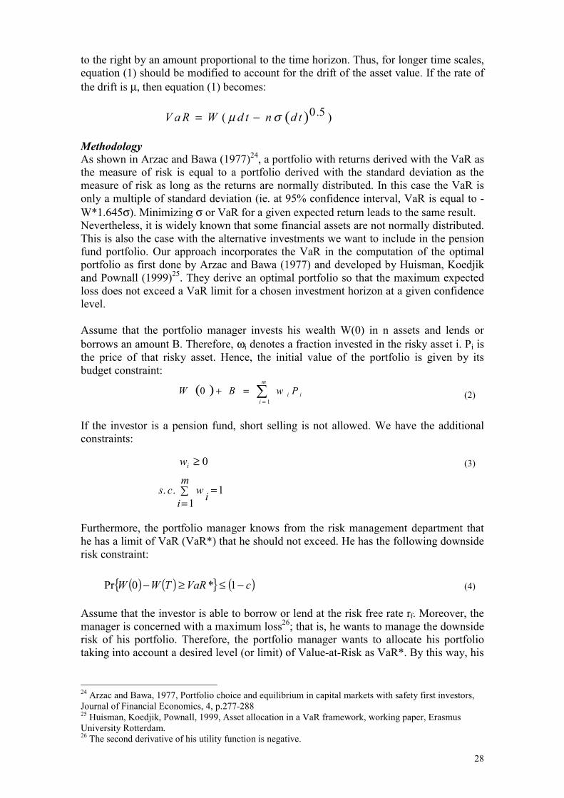
28
to the right by an amount proportional to the time horizon. Thus, for longer time scales, equation (1) should be modified to account for the drift of the asset value. If the rate of the drift is µ, then equation (1) becomes:
Methodology As shown in Arzac and Bawa (1977)24, a portfolio with returns derived with the VaR as the measure of risk is equal to a portfolio derived with the standard deviation as the measure of risk as long as the returns are normally distributed. In this case the VaR is only a multiple of standard deviation (ie. at 95% confidence interval, VaR is equal to -W*1.645σ). Minimizing σ or VaR for a given expected return leads to the same result. Nevertheless, it is widely known that some financial assets are not normally distributed. This is also the case with the alternative investments we want to include in the pension fund portfolio. Our approach incorporates the VaR in the computation of the optimal portfolio as first done by Arzac and Bawa (1977) and developed by Huisman, Koedjik and Pownall (1999)25. They derive an optimal portfolio so that the maximum expected loss does not exceed a VaR limit for a chosen investment horizon at a given confidence level. Assume that the portfolio manager invests his wealth W(0) in n assets and lends or borrows an amount B. Therefore, ωi denotes a fraction invested in the risky asset i. Pi is the price of that risky asset. Hence, the initial value of the portfolio is given by its budget constraint:
If the investor is a pension fund, short selling is not allowed. We have the additional constraints:
Furthermore, the portfolio manager knows from the risk management department that he has a limit of VaR (VaR*) that he should not exceed. He has the following downside risk constraint:
Assume that the investor is able to borrow or lend at the risk free rate rf. Moreover, the manager is concerned with a maximum loss26; that is, he wants to manage the downside risk of his portfolio. Therefore, the portfolio manager wants to allocate his portfolio taking into account a desired level (or limit) of Value-at-Risk as VaR*. By this way, his
24 Arzac and Bawa, 1977, Portfolio choice and equilibrium in capital markets with safety first investors, Journal of Financial Economics, 4, p.277-288 25 Huisman, Koedjik, Pownall, 1999, Asset allocation in a VaR framework, working paper, Erasmus University Rotterdam. 26 The second derivative of his utility function is negative.
( )V a R W d t n d t= −( . )µ σ 0 5
( ) ∑=
=+m
iii PwBW
10 (2)
s c w ii
m. . =
=∑ 1
1
0≥iw
( ) ( ) ( )cVaRTWW −≤≥− 1*0Pr
(3)
(4)
29
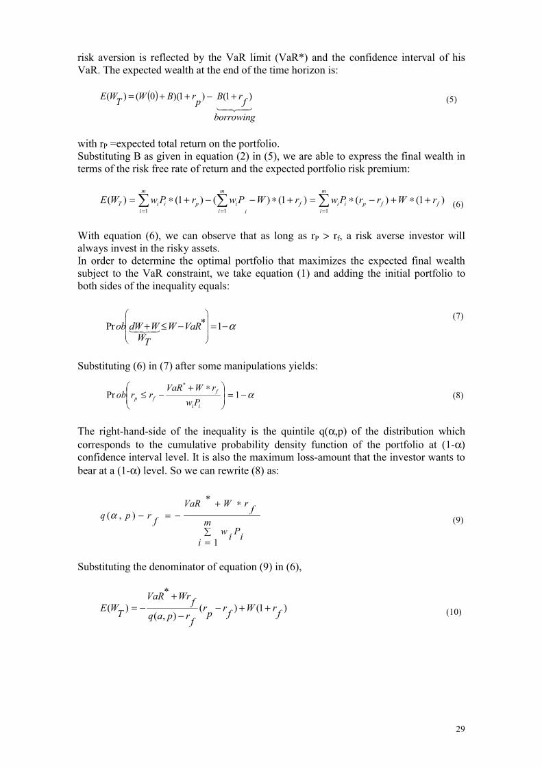
risk aversion is reflected by the VaR limit (VaR*) and the confidence interval of his VaR. The expected wealth at the end of the time horizon is:
with rP =expected total return on the portfolio. Substituting B as given in equation (2) in (5), we are able to express the final wealth in terms of the risk free rate of return and the expected portfolio risk premium:
With equation (6), we can observe that as long as rP > rf, a risk averse investor will always invest in the risky assets. In order to determine the optimal portfolio that maximizes the expected final wealth subject to the VaR constraint, we take equation (1) and adding the initial portfolio to both sides of the inequality equals:
Substituting (6) in (7) after some manipulations yields:
The right-hand-side of the inequality is the quintile q(α,p) of the distribution which corresponds to the cumulative probability density function of the portfolio at (1-α) confidence interval level. It is also the maximum loss-amount that the investor wants to bear at a (1-α) level. So we can rewrite (8) as:
Substituting the denominator of equation (9) in (6),
( )NMNLK
borrowingfrBprBWTWE )1()1)(0()( +−++=
∑ ∑∑= ==
+∗+−∗=+∗−−+∗=m
i
m
iffpiif
i
m
iipiiT rWrrPwrWPwrPwWE
1 11
)1()()1()()1()(
Pr *ob dW WWT
W VaR+ ≤ − = −
1 α
(5)
α−=
∗+−≤ 1Pr
*
ii
ffp Pw
rWVaRrrob (8)
∑
=
∗+−=−
m
i iPiw
frWVaR
frpq
1
*
),(α
)1()(),(
*)( frWfrpr
frpaqfWrVaR
TWE ++−−
+−=
(6)
(9)
(10)
(7)
30
Dividing by W,
Remember that VaR* is the Value at Risk limit that the investor wants to bear. This term can be seen as an additional constraint for the investor. The objective of the investor, concerned by the downside risk, is to maximize the expected return of his portfolio. Hence, he wants to maximize equation (11), which is equivalent to maximizing the ratio S(p):
So, S(p) equals the expected excess return on portfolio p divided by the expected loss on portfolio p that is incurred with probability (1-α). Note that the asset allocation process is thus independent of wealth. VaR is the Value at Risk of the portfolio p. Remember that this VaR is the Value at Risk of the optimal portfolio, which may not be the VaR limit that the investor has. As the risk is measured with the VaR, the denominator can be seen as a measure of regret since it measures the potential loss of investing in risky assets. S(p) is a measure of performance like the Sharpe ratio. The advantage of this measure is that it does not rely on any distribution assumptions and is therefore able to incorporate non-normalities in the portfolio allocation. The existence of non-normalities may lead to the choice of different portfolios. If we assume that returns are normally distributed and that the risk free is equal to zero, then, S(p) collapses to the classical Sharpe ratio. The optimal portfolio, which maximizes S(p), is independent from the desired level of VaR* (see equation (4)) since the measure VaR in (12) represents the optimal portfolio Value at Risk. The investor first allocates the risky assets by maximizing S(p). Then, he decides the amount of wealth to lend (or borrow) depending on how much of the portfolio's VaR is higher (or lower) compared to the VaR* limit. This is exactly the same as moving on the CML in a mean-variance setting27. The amount to lend or borrow in order to obtain the desired level of VaR* is obtained by substituting (2) in (9)
Rearranging and extracting B becomes
27 In a mean-variance setting, the investor computes the market portfolio w rf= − −1 1
γµ( )Ω and then
according to his desired level of volatility borrows at rf and places the proceed in the market portfolio if he wants to increase his risk (ie. he will move on the right on the Capital Market Line) or lends at rf by
( ) ( )( )
( ) )1()*0()),((*0
)0
( *ff
pS
f
fpT rrWVaRrpqW
rrWW
E +++−
−−=
α
( ) ( ) ( ) VaRrWrr
pqWrWrr
pSf
fP
f
fp
−−
=−−
=*0),(*0*0
)(max_α
(13)
BVaR W rr q p
WW VaR W r W r q p
W r q pf
f
f f
f
=+
−− =
+ − −−
* **( , )
*( * ) *( ( , ))*( ( , ))α
αα
2
q p r f
V a R W r fW B
( , )
* *α − = −
+
+
(12)
(14)
(11)
31
VaRfrWVaRVaRWB
+−=
*)(*
*
with VaR : optimal Value at Risk28 VaR*: Value at Risk limit for the investor When the desired level of risk (ie. VaR* ) is lower than the VaR of the optimal portfolio, the numerator will be lower than zero, B will be negative, so the investor will lend the amount B. The objective now consists in drawing the efficient frontiers based on this new framework, that is in the mean-Value-at-Risk theory. The only problem is to compute the Value-at-Risk without doing any assumption on the underlying distribution. We have to estimate the VaR analytically, that is the VaR is derived with the parameters characterizing the distribution of the returns. We use a Cornish-Fisher (1937)29 expansion to compute the VaR analytically30. It adjusts the traditional VaR31 with the skewness and kurtosis of the distribution:
with: zc: critical value for probability (1-α) S: skewness K: excess kurtosis The VaR is equal to:
Then, the modified VaR developed in this paper is equal to
σ
−−−+−+−µ= 2c
3cc
3c
2cc S)z5z2(
361K)z3z(
241S)1z(
61zWVaR
In formula (18), zc is equal to –2.33 for a 99% probability or to –1.645 for a 95% probability. The modified VaR allows us to compute the VaR for distributions with asymmetry and fat tails. Note that if the distribution is normal, S and K are equal to zero, which makes “z” to be equal to zc. We are, therefore, back to the normal case.
decreasing his exposure to risky assets if he wants to decrease his risk (ie. he will move on the left on the Capital Market Line) 28 VaR=Wq(α,p), with q(α,p)<0. So in the calculus we invert the sign of VaR in the numerator and at the denominator. 29 Cornish and Fisher, 1937, Moments and cumulants in the specification of distributions, Review of the International Statistical Institute, p.307-320. 30 David X Li, 1999, Value-at-Risk based on volatility, skewness and kurtosis, Riskmetrics Group, Working paper, derives also an analytical formula for confidence interval by using estimating functions. But with his formula, it was not possible to find a realistic one-side confidence level for negative returns. 31 Mina and Ulmer, 1999, Delta-Gamma Four Ways, Riskmetrics Group, provide four methods to compute the VaR for non-normally distributed assets: Johnson transformations, Cornish-Fisher expansion, Fourier method, partial Monte-Carlo. They found that Cornish-Fisher is fast and tractable, but sometimes not accurate with extremely sharp distributions.
(15)
2c
3cc
3c
2cc S)z5z2(
361K)z3z(
241S)1z(
61zz −−−+−+=
)( σµ zWVaR −=
(16)
(17)
(18)
32
5.3.3 Efficient frontier in a mean-modified Value-at-Risk setting In this section, we show the results obtained by applying the methodology explained above. We compute the efficient frontier and the optimal portfolio allocation for a Swiss pension fund assuming that the portfolio manager has a VaR* limit, that is, he does not want to loose more than x% each month at a probability of (1-α). The assets available for investment are the SPI (returns in CHF), the MSCI (returns in USD), the Salomon Brother Weighted Global Bond Index (returns in USD), the Salomon Brother Weighted Swiss Bond Index (returns in CHF) and the Hedge Fund Global Index (returns in USD). As previously done, we assume that perfect hedging is feasible and at no cost32. We use monthly data from January 1989 to June 1999. In order to compute the VaR, we use three different techniques: First, the returns of the indices (HFGI included) are assumed to be normally
distributed. Hence, the maximization of formula (12) in a mean-Value-at-Risk setting33 yields the same result as in a mean-variance setting. We compute a VaR at 95% and 99%34 confidence level.
The second technique uses formula (18). We maximize formula (12) and replace VaR with the modified VaR in formula (18). The modified VaR is computed at 95% and 99% confidence level.
The third technique consists in taking the empirical distribution: we compute the empirical VaR.
The three VaR techniques allow us to compute three different efficient frontiers. In the three cases above, we have the same constraints as for the mean-variance setting. That is, no short selling allowed, full investment constraint and the standard investment limits (see table 3). Figures 1 and 2 show the impact on the efficient frontier of a distribution with fat tails and asymmetric returns, which is the case with our Hedge Funds Global Index35.
32 ie.the forward rate is an unbiased estimator of the future spot rate 33 The mean will be on the vertical axis and the Value at Risk on the horizontal axis. 34 As it is a one tail measure, the critical values are respectively 1.645, 2.33. 35 Note that not only hedge funds may show asymmetry or fat tails distribution. for the monthly log returns of the SPI, from 2/1980 to 9/1997, excessK= 5.05, S= -0.98 are significant at 95%. So, during this period, this index is not significantly normally distributed as well.
33
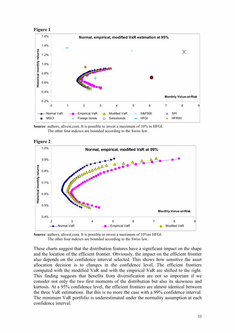
Figure 1
Source: authors, altvest.com. It is possible to invest a maximum of 10% in HFGI. The other four indexes are bounded according to the Swiss law.
Figure 2
Source: authors, altvest.com. It is possible to invest a maximum of 10%in HFGI. The other four indexes are bounded according to the Swiss law.
These charts suggest that the distribution features have a significant impact on the shape and the location of the efficient frontier. Obviously, the impact on the efficient frontier also depends on the confidence interval selected. This shows how sensitive the asset allocation decision is to changes in the confidence level. The efficient frontiers computed with the modified VaR and with the empirical VaR are shifted to the right. This finding suggests that benefits from diversification are not so important if we consider not only the two first moments of the distribution but also its skewness and kurtosis. At a 95% confidence level, the efficient frontiers are almost identical between the three VaR estimations. But this is no more the case with a 99% confidence interval. The minimum VaR portfolio is underestimated under the normality assumption at each confidence interval.
Normal, empirical, modified VaR estimation at 95%
0.2%
0.4%
0.6%
0.8%
1.0%
1.2%
1.4%
1.6%
0 1 2 3 4 5 6 7 8 9
Monthly Value-at-Risk
His
toric
al m
onth
ly re
turn
s
Normal VaR Empirical VaR Modified VaR S&P500 SPIMSCI Foreign bonds Swissbonds HFGI HFRWI
Normal, empirical, modified VaR at 99%
0.4%
0.5%
0.6%
0.7%
0.8%
0.9%
1.0%
2 3 4 5 6 7 8 9
Monthly Value-at-Risk
His
toric
al m
onth
ly re
turn
s
Normal VaR Empirical VaR Modified VaR
34
Both graphs clearly suggest that the level of the VaR is better estimated with the empirical VaR formula or with modified VaR than with the normal VaR. On the right hand side of the efficient frontiers, the modified VaR estimation underestimates the true VaR from 0.2% to 1.1% at 99% confidence level. At the 95% confidence level, the difference between the empirical VaR and the modified VaR estimation is never higher than 0.2% per month.
5.3.4 Conclusion Risk as measured by the empirical VaR or by the modified VaR is higher for all combinations of assets than captured by the use of standard deviation alone. This underestimation of risk will be even greater as the deviation from normality increases. The greater probability of extreme negative returns in the empirical distribution implies greater downside risk than is captured by the measurement of the standard deviation alone. These findings are particularly important in the case of some hedge fund investment strategies. It is important at this stage to highlight again that our hedge fund index is representative of the industry but not of an investment strategy in particular. If a Swiss pension fund tries to construct an optimal hedge fund portfolio, it may result in greater deviation from normality. Therefore, we have just shown the importance to go beyond the standard measure of risk like the standard deviation.
5.4 Optimal tangent weights in a mean-modified VaR setting The objective of this section is to determine the optimal weights of each asset class to be included in a portfolio of a Swiss pension fund. We have just seen that taking into account the non-normality of the distribution may have a significant impact on the efficient frontiers (on the level of risk). This is particularly true for hedge funds, where distributions may be far from normality for some investment strategies. Therefore, it is interesting to check if it is still interesting for a Swiss pension fund to invest in this type of financial instruments if we take into account the skewness and the kurtosis of the distribution. The optimal weights36, on the efficient frontier, are obtained by maximizing formula (12) for normal VaR, empirical VaR and modified VaR estimation:
with z obtained from equation (16). We assume a one month risk-free rate of return of 0.2%37. Then, if the distribution is assumed to be normal, maximizing (19) with the VaR at the denominator is the same as 36 Computing optimal weights here is the same as the computing tangent portfolio weights.
OOO NOOO ML
VaR
iiif
ifii
WzrwrW
rrwpS
∗−−∗
−∗=
∑
∑
=
=5
1
5
1
)*()(max_
σ(19)
35
maximizing a Sharpe ratio. But as soon as the distribution is assumed to be not normal, the maximization of formula (18) above will lead to other optimal weights. We still assume that the pension fund is not allowed to invest more than 10% of its wealth in hedge funds and regarding the other asset classes the same investment limits as before are kept (see table 3). No short selling is allowed and full investment constraint is assumed. The table below compares the weights for the tangent portfolio under normal distribution, under empirical distribution and under modified VaR when the Value-at-Risk is computed with a confidence level of 95%, 97.5% and 99%: Table 1 Optimal portfolio weights for different confidence levels of the Value-at-Risk
Value-at-Risk 1.76% 1.95% 1.81% 2.24% 2.27% 2.35% 2.80% 3.06% 3.08% Source: authors, altvest.com. It is possible to invest a maximum of 10% in HFGI.
The other four indices are bounded according to the Swiss law and as previously mentioned, see table 3.
Table 1 suggests that despite taking into account the third and the fourth moment of the distribution, efficient portfolios are still composed of the maximum 10% weight of HFGI, which is the maximum allowed. Hence, in figures 1 and 2, all the efficient frontiers (ie. from the minimum VaR portfolio to the highest expected return portfolio) are composed with 10% HFGI. This may be due to the fact that our Hedge Fund Global Index shows a very low level of standard deviation for the period under review. Note that the MSCI enters in no tangent portfolio, except at 99% for the empirical distribution. The poor performance of the MSCI and its high volatility over the 1989-1999 period explain that. Let us now check if the fact of adding a certain percentage of hedge fund investments is still valuable for the pension fund. We compare the efficient frontiers assuming, firstly, that no hedge funds are available for investment purposes and then assuming that a maximum of 2.5%, 5%, 7.5% and 10% may be invested in hedge funds. An efficient frontier is computed for each constraint. When the portfolio manager invests in hedge funds, the VaR is computed with the modified VaR approach. Moreover, it is not allowed to invest more than 55% in SPI, MSCI and HFGI all together38. The comparison of these portfolios is done at a 95% confidence level39 (ie. µ-1.645σ for the normal VaR) in the figure 3. The VaR of the LPP Pictet Index on figure 3 is the modified Value-at-Risk.
37 An annual average risk free return for the period January 1989-June 1999 of 2.4% divided by 12. 38 In 1999, the Swiss law allows to invest a maximum of 30% in the SPI and 25% in the MSCI. The sum of both is 55%. 39 The same kind of graphs have been obtained at 97.5% and 99% confidence levels.
36
Figure 3
Source: authors, altvest.com, Datastream. It is possible to invest a maximum of 10%in HFGI. HFGI is our hedge funds index composed with the 53 biggest hedge funds. Non-normality is taken into account through the modified VaR. The other four indices are bounded according to the Swiss law. Moreover, wSPI +wMSCI +wHFGI ≤55%. A monthly risk-free rate of 0.2% is assumed.
Figure 3 compares the efficient frontiers assuming that hedge funds are available for investment and taking into account non-normalities of the distribution through the modified VaR. Evidence is given that even if we take into account the first four moments of the distribution, investing in hedge funds allows shifting the efficient frontier to the left hand side. This graph suggests that the higher the constraint of maximum Hedge funds investments limit, the more the efficient frontier moves to the left. Again, it is important to highlight that it is not possible to generalize this result to all portfolios containing hedge funds. It is true for our hedge fund index. Table 2 shows the modified Sharpe ratios in a Mean-Value-at-Risk setting with assumption of normally distributed returns and non-normally distributed returns. Furthermore, we also assume a one month risk-free rate of returns of 0.2%. Table 2 Assumption of normal
distribution Non-normally distributed
returns Without
Hedge Funds Max 10% of Hedge Funds
Without Hedge Funds
Max 10% of Hedge Funds
Mod. Sharpe with VaR at 95% 0.2230 0.3010 0.2157 0.2874 Mod. Sharpe with VaR at 99% 0.1442 0.1894 0.1296 0.1693
Source: authors, altvest.com. It is possible to invest a maximum of 10% in HFGI. In order to compute the tangent portfolios, the other four index are bounded according to the Swiss law.
By taking the fourth moments of the distribution into account, the modified Sharpe ratio decreases. Non-normality of the SPI, the MSCI and the HFGI leads to a higher VaR, thus to a lower modified Sharpe ratio. Nevertheless, adding a max of 10% of our Hedge Funds Global Index leads to an increase of the modified Sharpe ratio (an increase in slope of 30%, from 0.1296 to 0.1693). It is important to highlight that our tests are based "in the sample" observations.
0.2%
0.3%
0.4%
0.5%
0.6%
0.7%
0.8%
0.9%
1.0%
1 2 3 4
Monthly Value-at-Risk
His
toric
al m
onth
ly re
turn
s
Max 0% of HFGI Max 2.5% of HFGI Max 5% of HFGIMax 7.5% of HFGI Max. 10% of HFGI LPP Pictet Index
Efficient frontiers with and without HFGI
37
In table 3, we test if the previously obtained results are valid at a 3 months horizon. A modified Sharpe ratio (ie. trimestrial returns divided by three months modified VaR)40 is computed with Hedge Funds available at a maximum level of 10%. Table 3 Non-normally distributed returns
With 0% HFGI With 10% HFGI Modified Sharpe ratio 0.0062 0.0090 Source: authors, altvest.com. The increase in the modified Sharpe ratio, if we also assume that the risk-free rate is equal to zero, is equal to 45% which is higher than the modified Sharpe ratio obtained with monthly data. This is explained by the fact that the trimestrial HFGI returns distribution is less skewed with lower fat tails (ie. S=-1.09, excess K=2.25) with respect to the monthly returns distribution (S=1.40, excess K=4.65). So including 10% of HFGI in the portfolio reduced the impact on the modified VaR with respect to the monthly returns framework.
5.5 Verifying the robustness of the results obtained We constructed a Hedge Fund Global Index composed of 53 large and representative Hedge Funds. To test the robustness of our results, we proceeded in two steps: Firstly, we compare the results obtained with our HFGI with another global well-
diversified Hedge Funds index. We select the Hedge Fund Research Weighted Composite index (HFRWI) from January 1990 to June 1999. An analysis of non-linear correlation and the efficient frontier impact are done with the HFRWI.
Secondly, we perform an out-of sample analysis.
5.5.1 Efficient frontiers with the HFR Index Figure 4 below compares the returns of the HFRWI with those of the HFGI during the period starting in January 1990 to June 1999. This figure can be compared to the figure 3 obtained in section 3.3.2 where we compare the returns of our constructed HFGI with the returns of the LPP Pictet index.
40 Longer horizon will be difficult as with three months horizon, our sample is reduced to 42 data. Moreover, if we assume that the Hedge Funds can be seen as barrier options, with the impact of leverage and margin calls, dealing with higher horizon (ie. smoothing the returns) is specially dangerous at our mind.
38
Figure 4
Source: authors, HFR, Datastream. LPP Index returns are sorted from lower to higher. The respective HFR Index returns are added. We observe that the result in figure 4 is almost similar compared to the figure 3 in section 3.3.2. The HFR Index is not correlated to the LPP Index till –1.5% for the LPP Index. After both indices decrease together on the left of the graph. Finally, the comparison of the efficient frontiers in a mean-Value-at-Risk setting leads to approximately the same level of modified VaR. The weights on the frontier are almost the same as with our constructed HFGI. The hedge funds weights increases until a maximum of 10% and at that point the portfolio is almost the most diversified one. Figure 5
Source: authors, HFR, Datastream. The 3 frontiers take into account volatility, skewness, kurtosis. Based on the results obtained above, we conclude that the construction of our Hedge Funds Global Index was representative for an average of the hedge funds strategies and our conclusions are robust. By taking into account skewness and kurtosis of each of the five indexes of our portfolio, it is possible to decrease the Value-at-Risk which accounts
for volatility skewness and kurtosis significantly or for the same modified VaR to increase the expected returns.
5.5.2 Out-of-Sample in a mean-modified VaR setting Introduction In section 5.4, figure 3 we show that the efficient frontier is always shifted to the left when we introduce a percentage of hedge fund investment in the pension fund portfolio. This is true even when we take into account the skewness and the kurtosis of the distribution. We concluded that the diversification benefits obtained by investing in this new asset class compensate the impact of the non-normality of its returns' distribution. This test is based on an in-the-sample observation. Let us perform now an out-of-sample analysis.
Methodology We split our sample in two. The first sample data, from January 1990 to December 1995, is used to compute the parameters in order to maximize equation (19). We obtain the weights of the optimal portfolio. Then, these weights are used to compute the returns over the second period, that is from January 1996 to June 1999. We perform three maximizations with the following assumptions: No hedge funds are available, Hedge funds are available with an investment limit of 5%, Hedge funds are available with an investment limit of 10%. Furthermore we assume a zero risk free rate of return. The assets available for investment are the SPI (returns in CHF), the MSCI (returns in USD), the Salomon Brother Weighted Global Bond Index (SBWBI), returns in USD, the Salomon Brother Weighted Swiss Bond Index (SBSBI), returns in CHF and the Hedge Fund Research Weighted Composite Index (HFRWI), returns in USD. We decide to take the HFRWI to do this out-of-sample analysis to avoid the low level of standard deviation shown by our constructed Hedge Fund Global Index. It is important to underline that the constructed portfolio are fully hedged. The currency fluctuations have no impact on the level of risks of the HFRWI, MSCI or SBWBI. Investment limits are the same as before, that is 30% for the SPI, 25% for the MSCI, 20% for the SBWBI and 100% for the SBSBI. Full investment and no short selling constraints are also applied. Results We obtain the following weights with the optimization: Table 4 Asset class No Hedge Funds available Hedge Fund investment
limit of 5% Hedge Fund investment
limit of 10% HFWI 0% 5% 10%
SPI 5% 3% 1% MSCI 0% 0% 0%
SBWBI 20% 20% 20% SBSBI 75% 72% 69%
Total 100% 100% 100%
40
Table 4 shows that hedge funds take the place of swiss bonds and of the SPI. Once the weights of the tangent portfolios are obtained, we compute the monthly returns that each portfolio would have yielded from January 1996 to June 1999. Based on these monthly returns, we compute the average return over the period and the modified VaR. We obtain the following results: Table 5 Average
return Modified
VaR Modified
Sharpe Ratio Portfolio with 0% HF 0.53% 2.37% 0.223 Portfolio with 5% HF 0.54% 2.18% 0.247
Portfolio with 10% HF 0.55% 2.03% 0.271 Table 5 shows that the average return we obtain is improved by adding hedge fund investments in our portfolio. The level of risk, measured with the modified VaR is decreased by adding hedge funds. This one path out-of-sample test shows that there is clearly a benefit in investing in hedge funds even if we take into account the non-normality features of the hedge funds.
6 Allocation in a downside-risk setting The Hedge Fund strategies are characterized by having correlation coefficients with traditional investments which are not constant over time and the fact that they increase during markets downturns41. By using the Lower Partial Moment (LPM), it is possible to take this last fact into account as the LPM measures the deviation below a target. The LPM can be useful in order to compute efficient frontiers and optimal allocations in Hedge Funds strategies42. With this method, the investor is interested in the distribution below a target return (for example, below –1% monthly return). The LPM for an empirical discrete distribution is given by the following optimization:
subject to the following constraints
n=1 if the aim is to minimize the deviation below the target returns RT n=2 if the aim is to minimize the variance below the target ∑wiE(Ri)=R* ∑wi=1 wi≥0
41 Refer to Chapter 2 for strategies correlation analysis. 42 See W.V.Harlow, 1991, Asset allocation in a downside-risk framework, Financial Analyst Journal, for the development of the concept of Lower Partial Moment. They found that by using LPM, instead of mean-variance theory for optimization purpose, it is possible to decrease the risk of a portfolio and to maintain or even improve the expected returns.
∑<
−
−=
TR
TRpR
npRTR
mnLPMw 1
1minmin_ (1)
41
with m: the number of return observations n: describe the type of moment Rp: distribution returns RT: fixed return target. R* represents the level of returns to reach by minimizing the target shortfall (if n=1) or the under-target variance (if n=2). The type of moment “n” allows taking the utility of the investor into account. LPM1 is valid for an investor with utility U’(.)>0 and U’’(.)<0. LPM2 is valid for an investor that displays skewness preference (U’(.)>0, U’’(.)<0 and U’’’(.)>0). If the returns' distribution of the assets is normally distributed, the weights wi and the efficient frontiers will be the same as in a mean-variance setting. But with the Hedge Funds, the LPM will describe the behavior of a distribution below a target which is of interest as almost all Hedge Funds strategies distribution have significant skewness and kurtosis. The optimization of equation (1) is done with the HFGI, the SPI, the MSCI, the SBWGI (ie. foreign bonds index) and the SBWSB (ie. Swiss bonds index). We use the LPM with moment of order n=2, as the Swiss pension funds can be characterized with an exponential utility function with U’’’(.)>0. The objective is to show what the impact of characterizing the risk of the Hedge Funds is with the variance below a negative return43. It is possible, as in Harlow (1991), to reduce the risk level of a portfolio, obtained with a classic mean-variance optimization. In our case, the risk is the variance under a target returns fixed at –1%. By using the shortfall risk, it is possible to lower the LPM2 from 1.05% to 1.01%44 for the portfolio with the minimum lower partial moment of order 245. Note that this reduction in the risk level is not obtained by decreasing the HFGI weights, but by slightly decreasing or increasing some percentage allocation of SPI and MSCI weights46. As our Hedge Funds Global Index's weight is bounded at 10% in the optimization and the index does not show a wide left fat tail (excess kurtosis of 4.46), it cannot influence the shortfall risk LPM2 measure47 too negatively.
43 We set the target returns at –1% as many HFR strategies (see Chapter 2) have significant increasing positive local correlation with LPP Pictet Index below this target. 44 These two numbers represent the monthly semi-standard deviation below –1%. To obtain the annual one, multiply by square-root of 12. 45 Our results are less spectacular than those obtain by Harlow(1991), this is due to the weights constraints included in the optimization. 46 The SPI and MSCI distribution are not statistically normally distributed for January 1989-June 1999 monthly returns. 47 We test the optimization with max. 100% of HFGI. It was possible to decrease the LPM2 risk measure, on average from 10%, by minimizing it compare to a mean-variance optimization.
42
Figure 1
Source: authors, altvest.com, datastream. A maximum of 10% is possible to invest in our HedgeFunds Global Index. The other four indexes are bounded according to the Swiss law. The minimum risk portfolio has an expected returns of 0.63%/month.
Figure 1 above shows the optimal weights of the mean-LPM2 frontier. The weights are not far from those obtained under a mean-variance optimization. Nevertheless, with the variance measure the risk is underestimated. The lower partial moment method will be preferred for an investor who is concerned only on the negative portion of the Hedge Funds distribution. This investor does not care about the shape of the positive returns distribution. This investor also desires not to deviate too much from a negative target returns level. The cons of this method is that it is necessary to have sufficient number of observations under the negative target level in order to obtain statistically reliable LPM1 or LPM2.
7 Conclusion We have shown that the risk of alternative instruments like hedge funds is not properly measured with the variance of the returns. This is due to the non-normal distribution of the returns. We performed our tests using monthly data from January 1989 to June 1999. It is important to observe that the returns of the MSCI have been low for this period (ie. an average of 0.71% over the period under review). This has an important impact on our results. This index is always under weighted. Based on the investment constraints included in our optimizations and considering these low MSCI returns, further developments could be to perform optimizations taking into account expected returns instead of historical returns48.
48 For example, use an inverse optimization to compute the implied returns coming from the world market.
Optimal weights by minimizing LPM2 (target -1%) with max. 10% of Hedge Funds
0%
10%
20%
30%
40%
50%
60%
70%
80%
90%
100%
0.48
%
0.50
%
0.52
%
0.54
%
0.56
%
0.58
%
0.60
%
0.62
%
0.64
%
0.66
%
0.68
%
0.70
%
0.72
%
0.74
%
0.76
%
0.78
%
0.80
%
0.82
%
0.84
%
0.86
%
0.88
%
Historical monthly returns
Wei
ghts
HFGI SPI MSCI Foreign bonds Swiss bonds
43
Mean-variance is not available when the investor is risk averse, which is the case of the pension funds. So, one has to use another approach which accounts for the non-normality of the returns. We developed and applied two techniques for portfolio asset allocation, which takes into account the non-normality of the returns' distribution, the modified Value-at-Risk and the Lower Partial Moment. Even by applying the modified Value-at-Risk which corrects for the normality, it is still worth to invest in a well diversified Hedge Funds portfolio. To compute the risk of a non-normal portfolio, with the volatility only, underestimates the risk by 12% to 40% at a VaR level of 99%. The effect of adding 10% of a well diversified hedge funds portfolio in a swiss pension fund hedged portfolio decreases the risk, measured with the modified VaR, by 19% to 40% at a VaR level of 99%. Thus, an investment in a diversified hedge funds portfolio is clearly interesting. But the price of the survivorship bias and the price of the liquidity of the hedge funds have not been taken into account till yet. This will have a negative impact on the historical return delivered by the hedge funds. The results obtained under the modified VaR are confirmed with the minimization of the Lower Partial Moment (n=2) below a target of –1%.
44
Part 2 Hedge Fund's characteristics analysis
8 Performance analysis of Hedge Funds
8.1 Introduction In the first part, we constructed our own hedge funds index. The objective was to create a replicable hedge funds portfolio which was representative of the global industry. In this chapter, we analyze the characteristics of ten hedge funds styles like the distribution of their returns and their linear correlation with a traditional portfolio. The objective consists in identifying the characteristics of each hedge funds style in order to be able to construct an optimal hedge fund portfolio taking into account the objective of the investor. The analysis we are doing in this second chapter is valid for all investors, not only for pension funds investors. The choice between several hedge funds or strategies is difficult when an investor wants to create a hedge fund portfolio. We will show that the classical linear correlation are not reliable with hedge funds. Some techniques will be proposed as non-linear regressions, non-linear correlation, pricing the option incentive fee and pricing the liquidity risk. The paper is divided into the following parts. Section 9 describes in short the different Hedge Funds strategies. Section 10 measures the historical returns and risks of these Hedge Funds strategies. Section 11 analyzes each Hedge Funds strategies with the help of correlation and regressions and section 12 presents the conclusions.
8.2 Definition Hedge Fund indices differ widely in purpose, composition and weightings. The major differences relate to management staffing, performance determination and strategies. For the purpose of this article, we use indices constructed and provided to us by Hedge Fund Research, Inc.(HFR), a firm specialized in research and analysis of hedge funds and alternative investment strategies. Performance is net of all fees for all funds and is defined as being the equally weighted mean return of the reporting hedge funds' results. In the following section, we briefly analyze the most important investment strategies: Convertible Arbitrage: involves purchasing a portfolio of convertible securities,
generally convertible bonds and hedging a portion of the equity risk by short-selling the underlying common stock. Certain managers may also seek to hedge interest rate exposures under some circumstances. Most managers employ some degree of leverage, ranging from zero to 6:1.
Merger Arbitrage: funds invest simultaneously in long and short positions in both companies involved in a merger or acquisition. In stock swap mergers, the Hedge Funds are typically long the stock of the acquired company and short the acquiring company. In the case of a cash tender offer, the Hedge Funds are seeking to capture the difference between the tender price and the price at which the acquired company
45
is traded. Profits are made by capturing the spread between the current market price of the target company and the price to which it wil appreciate when the deal is completed. The risk is that the deal fails.
Emerging markets: funds invest in securities of companies or the sovereign debt of developing or “emerging” countries. This style is more volatile not only because emerging market are more volatile than developed markets, but because most emerging markets allow for only limited short selling and do not offer a viable futures contract to control risk. This suggests that Hedge Funds in emerging markets have a strong long bias.
Equity hedge: investing consists of a core holding of long equities hedged at all times with short sales of stocks and/or stock index options. The short position has three purposes. First, it is intended to generate as well alpha. Stock selection skill for short stocks can result in doubling the alpha. An equity hedge manager can add value by buying winners and selling losers. Second, the short position can serve the purpose of hedging market risk. Third, the manager earns interest on the short position.
Equity non-hedge: funds are predominately long term equities, although they have the ability to hedge with short sales of stocks and/or stock index options. The leverage is created by borrowing money or by using derivatives. Some strategies are long stock index futures or buying stocks, using them as collateral to borrow money (50%) which is then reinvested in more stocks.
Event driven: also known as “corporate life cycle” investing. This involves investing in opportunities created by significant transactional events, such as spin-offs, changes in ownership, bankruptcies, reorganizations, share-buy-backs and recapitalizations. The securities prices of the companies involved in these events are typically influenced more by the dynamics of the particular event than by the general appreciation or depreciation of the debt and equity markets.
Market Neutral: seek to profit by exploiting pricing inefficiencies between related equity securities, neutralizing exposure to market risk by combining long and short positions. Market neutral portfolios are designed to be either beta-neutral, currency-neutral or both.
Fixed Income: groups all strategies together, which can be performed with fixed income instruments like arbitrage, convertible-, diversified-, high yield- and mortgage bonds.
Macro: involves leveraged bets in liquid market on anticipated stock market price movements, interest rates, foreign exchange and physical commodities. They pursue a base strategy such as long/short or future trend following to which highly leverage bets in other markets are added a few times each year. They move from opportunity to opportunity and from trend to trend. Macro funds make their money by anticipating a price change early and not by exploiting market inefficiencies.
Short selling: involves the sale of a security not owned by the seller with the intention of buying it back later at a lower price. In addition the short seller earns interest on the cash proceeds from the short sale of stock. Given the extensive equity bull market, short selling strategies have not done well in the recent past. Technically, a short sale does not require an investment, but it does require collateral.
CTA: Commodity Trading Advisors are investing in commodity and financial futures. For example, two of the used techniques are long/short stock index futures based on quantitative or technical trend following indicator with stop loss limit, or stock index arbitrage. We include them in the analysis, even though they are not considered being Hedge Funds by the practitioners.
46
8.3 Performance analysis The analysis covers the period January 1990 till June 1999, based on monthly observations. We obtained the following results: Table 1 µµµµ σσσσ S K RMAX RMIN ρρρρLPP
Convertible Arbitrage
0.92% 1.04 -1.46 3.18 3.3% -3.1% 0.44
Merger Arbitrage
1.00% 1.37 -3.21 13.7 2.9% -6.4% 0.46
Emerging Markets
1.36% 4.64 -1.16 4.31 12.3% -21.0% 0.59
Equity hedge
1.73% 2.36 -0.50 1.15 7.2% -7.6% 0.51
Equity non-hedge
1.66% 3.83 -0.82 1.79 9.5% -13.3% 0.59
Event Driven
1.35% 1.96 -1.78 7.34 5.1% -8.9% 0.61
Market neutral
0.87% 0.90 -0.09 0.55 3.5% -1.6% 0.07
Fixed income(Total)
0.98% 1.06 -0.58 6.05 5.3% -3.2% 0.49
Macro
1.59% 2.67 0.10 0.16 7.8% -6.4% 0.55
Short selling
0.22% 5.57 0.30 0.73 19.4% -16.2% -0.51
CTA 0.66% 2.76 0.44 0.35 10.0%
-5.5% -0.16
µµµµ : arithmetic monthly mean returns σσσσ : monthly standard deviation S : skewness 49 K : excess kurtosis 50 RMAX : maximum monthly returns over the period RMIN : minimum monthly returns over the period ρρρρLPP, BVG 51: linear correlation coefficient between the hedge fund strategy and the LPP Index Some interesting conclusions can be derived from table 1. First, all strategies achieve positive monthly mean returns. If we focus on a classical Sharpe ratio (i.e. mean returns divided by the standard deviation), the worst strategy is, by far, the short selling one, which is consistent with the stock market behavior of the last ten years. The best one is the market neutral, mainly because of its low level of standard deviation. If we look at the skewness and the kurtosis indicators, we observe that almost all strategies have a negative skewness52 and a positive excess kurtosis, except for the macro, short-selling and the CTA strategies. This means that negative returns will deviate from normality, 49 The skewness measures the asymmetry of a distribution. A normal distribution has a skewness of zero. 50 The kurtosis measures returns which are highly positive or highly negative with respect to the other returns. In other words, the kurtosis is a measurement of the fat-tailness of a distribution. A normal distribution has an excess kurtosis of zero. 51 The LPP Index or BVG Index is the Index constructed by Pictet & Cie (Geneva) and represents the Benchmark Index for a Swiss institutional investor. Typically, this Index does not include more than 30% of the SPI, 25% of the MSCI, 20% of the Salomon Brother Global Bond Index. 52 A negative skewness implies that the distribution has a long left tail. Risk averse investor does not like negative skewness.
47
especially on the downside, except in the case of the macro and short-selling strategies. The Merger Arbitrage is deviating the most from normality, the skewness and the kurtosis being significant53. Finally, the linear correlation with the LPP/BVG portfolio is an important indicator for the investors. Many pension funds look for diversification benefits when they decide to invest in alternative instruments. Therefore, asset allocation advisors construct a portfolio with a low correlation level, although for us this is not the right measure . With this objective in mind, the short selling, Convertible Arbitrage, CTA and market neutral strategies are interesting. The short selling strategy is an insurance, which some investors include in their portfolio. Like any other insurances, it has a price. In this case, the price consists of two factors, firstly the low level of return, at least when the markets of traditional instruments are bullish and secondly, the high level of standard deviation shown by the short selling strategy. It is interesting to observe that portfolio insurance can also be achieved by buying some put options, but not at the same costs and the same payoffs. In the next section, we will test nine of these strategies to determine which ones are adding diversification to a Swiss pension fund portfolio.
8.4 Local regression analysis The standard linear correlation is not appropriate, if we want to compare two distributions, of which the latter is not a normal one54. This is the case with the above Hedge Funds strategies, exceptions are the Macro and Short-Selling. Having two normally distributed assets is as well not sufficient to claim that a combination of both will be normally distributed. You must be, as well, convinced that they have jointly a multivariate normal or elliptical distribution55. An actual assessment of the correlation is fundamental for the creation of an optimum hedge fund portfolio. This is also true, if we want to take into consideration the investor's objectives. In the case of a pension fund, the common objective is to have a portfolio of hedge funds with a low correlation level, as compared with traditional investments. The objectives of this section are, firstly, to analyze the correlation between the LPP and the HFR indices using a methodology, which takes into account the non-linear relationship between both instruments and, secondly, to analyze the payoff structure of the HFR indices. The methodology being used is the local regression analysis. We shall show that four HFR strategies56 out of nine result in concave payoffs as compared to the LPP index. This means that the slope of the local regression decreases, when the LPP index returns increase. When LPP returns decrease, the HFR returns decrease at an even higher proportional rate. Moreover, when the relation is statistically not linear between both series (as in the four case cited above), the classical correlation coefficient correlation is misleading and will, in the case of convexity relation, give a higher correlation during markets downturns. 53 Only the Macro, the Short Selling and the CTA strategies have a normal distribution based on the Jarque-Berra statistics. 54 See appendix 2 for a theoretical demonstration. 55 Embrechts, Mc Neil, Straumann, Correlation and dependance in risk management: properties and pitfalls, ETH Zurich & RiskLab, Working paper. 56 HFR Weighted Composite Index, HFR Fixed Income, HFR Convertible Arbitrage, HFR Event Driven
48
8.5 Methodology We perform a local regression analysis on 9 different HFR investment styles (included an equally weighted Hedge Funds index) and the CTA strategy57. For each style selected, we first perform a Loess Fit analysis using a statistical software58. Loess Fit is a technique, which displays local polynomial regressions with the bandwidth based on nearest neighbors. Briefly, for each data point in a sample, the software fits a locally weighted polynomial regression. It is a local regression since it uses only the subset of observations, which lies in the neighborhood of the point fitting the regression model. We obtain a picture of local regressions between the LPP index and a hedge fund investment strategy. This picture helps us to identify the best way to do the regression, that is, with the help of the standard linear regression, by means of a quadratic regression or finally with aid of a polynomial third degree regression. The significance of the local regressions59 is verified using the adjusted R2. The adjusted R2 gives us the explanatory power of the local regression taking into account the number of independent variables. In our case, the independent variable is always the LPP Index. Therefore, the higher the adjusted R2, the more important the correlation between the LPP Index and the HFR strategy becomes. Moreover, we show that the parameters of the non-linear regressions are stable throughout time60.
8.6 Results HFR Weighted Composite Index (HFRWC) analysis This index is an equally weighted index of all Hedge Funds based on the HFR database. It is long biased. Figure 1 below shows the local regression obtained with the Loess Fit technique. We observe that the payoff of the HFR Weighted Composite Index is concave compared to the LPP61 index. The straight line in figure 1 corresponds to a 100% investment in the LPP index, considering that our reference asset is the LPP index. Furthermore, figure 1 suggests that the explanatory power of the linear regression can be improved upon by using a quadratic regression.
57 We have excluded Emerging markets which are not well defined in term of strategy, excluded Equity hedge strategies which are similar to Equity non-hedge, but with lower volatility and lower kurtosis. 58 For more information on local regression analysis, see Chambers, Hastie, Statistical models in S, 1992, Chapter 8, Wadsworth & Brooks. 59 We use Newey-West regression, which adjusts for autocorrelation and heteroskedasticity. 60 To do that, the period January 1990-June 1999 is divided in two equal sub-periods. A Chow-test which follows an F-distribution with 3 and 122 degrees of freedom is performed. 61 Remember that the LPP index is the index constructed by Pictet & Cie (Geneva) and represents the benchmark index for a Swiss institutional investor. Typically, this index consists of not more than 30% SPI, 25% MSCI, 20% Salomon Brother Global Bond Index.
49
Figure 162 Figure 1 shows that the HFRWC generates a slightly improved payoff, as compared to the LPP index, between -4% and +2% monthly LPP index returns. Table 1, (see appendix), shows the result of a quadratic regression between the HFR weighted composite index and the LPP index. The explanatory power of the regression (ie. adjusted R2 =0.42) is good. It is equivalent to a correlation coefficient of 0.65. If we assume that the HFRWC can be replicated and that the investor wants to diversify his standard portfolio, we notice that investing in the HFRWC is not optimal. This is not surprising, considering that the HFRWC is long biased. According to the Chow test63, the coefficients of the regression above are stable through out the time period at 99%. HFR Total Fixed Income Index (HFRFI) analysis This index includes arbitrage-, convertible-, diversified-, high yield- and mortgage-backed strategies in the fixed income area. Figure 2 shows the moving correlation between the HFRFI index and the LPP index. The moving correlation is a measure of the sensitivity of a portfolio to negative and positive returns. We take the 30 worst index (LPP) returns and calculate the correlation with the 30 respective Hedge Funds strategy (HFRFI) returns. Thus we are able to obtain one correlation coefficient. Then, we move the window by one month and recalculate the correlation coefficient. The graph shows firstly, that the correlation is not stable throughout time and secondly, that the correlation level is in general low, except for the extreme negative LPP index returns.
62 One interpretation of this graph is that the investor would have been better of investing in the Hedge Fund Strategy, when the concave curve was situated above the flat line. 63 The Chow-test, which measures the stability of the quadratic regression between two sub-periods (ie. Jan.1990-Sept.1994 and Oct.1994-June 1999), is equal to 3.06. The critical level of this Chow-test F(3,122) is 3.95 at 99%.
-0.10
-0.05
0.00
0.05
0.10
-0.06 -0.04 -0.02 0.00 0.02 0.04 0.06
LPP Index monthly returns
HFRWCI monthly returns
LOESS Fit (degree = 3, span = 1.0000)
50
Figure 2 Moving correlation between LPP Pictet Index and HFR Total Fixed Income Index over
30 observations
-0.6
-0.4
-0.2
0
0.2
0.4
0.6
0.8
-1.1
%
-0.7
%
-0.5
%
-0.4
%
-0.2
%
-0.1
%
0.0%
0.3%
0.6%
0.7%
0.8%
0.9%
1.0%
1.2%
1.4%
1.4%
1.6%
1.7%
2.0%
2.1%
2.3%
2.4%
Historical returns
Line
ar m
ovin
g co
rrel
atio
n
As mentioned by Fung and Hsieh (1999)64, the fixed income arbitrage strategy produces stable returns with low dispersions65. They argue that Arbitrage Fixed Income managers are not capturing mispricings, but that they sell economic disaster insurance. When the market is quiet, the managers perform well and poorly in volatile markets. For example, when the liquidity dried up in the months September, October and November 1998, the HFR Total Fixed Income Index lost –3.1%, -1.8% and –3.2% respectively. This fact is confirmed by Figure 3, where the slope for LPP returns below -1% of the regression, dramatically increases. Figure 3 Based on figure 3 and on the statistical Chow test, we performed two different regressions: one regression for index returns between –5%/month and +0.5%/month and another regression for index returns between 0.5%/month and 4.5%/month. The first regression has a quadratic form and the second a linear one with a slope of 0.2. A significant quadratic regression, with an adjusted R2 of 47%, below a return of 0.5%, means that the investor becomes more and more exposed, when the index returns turn
64 W.Fung, D.H.Hsieh, A primer on Hedge Funds, March 1999, Working paper, Duke University. 65 The empirical Value-at-Risk at the 95% level for the HFR Fixed Income Arbitrage and for the HFR Total Fixed Income is –2.58% and -0.66% respectively.
-0.04
-0.02
0.00
0.02
0.04
0.06
-0.06 -0.04 -0.02 0.00 0.02 0.04 0.06
LPP Pictet Index monthly returns
HFR Fixed Income monthly returns
LOESS Fit (degree = 2, span = 1.0000)
51
negative. This strategy can be seen as buying 0.2 LPP Indexes and selling put options with strikes further and further out-of-the-money66. Table 2 in the appendix shows the explanatory power of the first quadratic regression to be good (47%). Therefore, the correlation coefficient, considering only the negative returns, equals 0.69. This is a significant increase, as compared to the classical correlation coefficient between the index (obtained in table 1, which was equal to 0.49), which takes all the returns into consideration in a linear way. HFR Macro Index (HFRMA) analysis The macro managers anticipate market movements by using top-down approaches. Historically, they achieve high yearly returns. Furthermore, they argue that their investments have low linear correlations with traditional instruments. As figure 4 shows, the moving correlation is again not stable and low, except for LPP returns below -0.4% and between 1.4% and 2%. Figure 4
Moving correlation between LPP Pictet Index and HFR Macro Index over 30 observations
-0.2
-0.1
0
0.1
0.2
0.3
0.4
0.5
0.6
-1.1
%
-0.7
%
-0.5
%
-0.4
%
-0.2
%
-0.1
%
0.0%
0.3%
0.6%
0.7%
0.8%
0.9%
1.0%
1.2%
1.4%
1.4%
1.6%
1.7%
2.0%
2.1%
2.3%
2.4%
Historical returns
Line
ar m
ovin
g co
rrel
atio
n
Figure 5 shows that, if there is a significant relationship, it should be a linear one. We performed a linear regression between the HFRMA Index and the LPP index and found a significant relationship with an adjusted R2 of 0.2967. The constant of the linear regression is equal to 0.009 and the coefficient of the LPP index equals to 0.904. This means that, by investing in a macro Hedge Fund, the investor will be exposed to 0.904 of the returns of the LPP index68.
66On average as the adjusted R2 is not equal to 100%. 67 Fung and Hsieh, 1999, A primer on Hedge Funds, found that the payoffs of the macro strategies can be seen as a long position in the SP500, short calls in-the-money and long put positions. But they do not provide a local linear coefficient in order to prove the statistical validity of their conclusions. 68 On average as the adjusted R2 is not equal to 100%.
52
Figure 5 HFR Market Neutral (HFRMN) analysis By definition this strategy should have a beta of zero with the market. The market could be equity, bond, commodity, currency, real estate, private equity, ... markets. By trading on the long and short sides, in theory, they should neutralize their exposure to each of these different markets. We will show that this theoretical beta of zero, in a linear regression, is valid only on the LPP negative side. Figure 6 shows that the relation between HFRMN and the LPP Index is not defined. When the LPP Index gets monthly returns higher than ~1.7%, the HFRMN Index gets returns lower and more and more small (all the part on the left of the straight line). When the LPP Index returns are negative, the HFRMN Index performs very well and is always positive. Figure 6 Now, we have to see if this graph is significant and what is the relation between both indices. A regression to the power three is done, in table 4 in the appendix, which shows that the relation between both indices is small (adjusted R2 = 1.2%). All the coefficients of the regression to the power three are significant at 95%, as the absolute t-stat are higher than 1.96.
-0.10
-0.05
0.00
0.05
0.10
-0.06 -0.04 -0.02 0.00 0.02 0.04 0.06
LPP Pictet Index monthly returns
HFR Macro Index Monthly returns
LOESS Fit (degree = 1, span = 1.0000)
-0.02
0.00
0.02
0.04
-0.06 -0.04 -0.02 0.00 0.02 0.04 0.06
LPP Index monthly returns
HFRMN monthly returns
LOESS Fit (degree = 3, span = 0.9000)
53
In conclusion, this strategy provides really good diversification for a swiss pension fund with a non-linear correlation of 0.11, no exposure at all on the downside, an annual volatility of 3.2%69 and an historical annual return of 10%. HFR Equity Non-Hedge (HFRNE) analysis This strategy has similar features70 as the HFR Equity Hedge Index, from a statistical point of view, except that the HFRNE return distribution is more dispersed. Figure 7 shows an increasing correlation coefficient with extreme negative LPP Index returns. The five worst LPP returns correspond to the four worst HFRNE Index returns. So, the HFRNE Index provides increasing exposure, for a Swiss pension fund, to extreme left tailed LPP Index return events. Figure 7
Moving correlation between LPP Pictet Index and HFR Non-Hedge Index over 30 observations
-0.3
-0.2
-0.1
0
0.1
0.2
0.3
0.4
0.5
0.6
0.7
0.8
-1.1
%
-0.7
%
-0.5
%
-0.4
%
-0.2
%
-0.1
%
0.0%
0.3%
0.6%
0.7%
0.8%
0.9%
1.0%
1.2%
1.4%
1.4%
1.6%
1.7%
2.0%
2.1%
2.3%
2.4%
Historical returns
Line
ar m
ovin
g co
rrel
atio
n
Figure 8 shows the payoffs of the HFRNE index as compared to the LPP Index. By using a polynomial third degree regression, the shape of the relation is concave for negative LPP returns and convex for positive LPP returns. The slope of the concave regression varies between 2.6 and 1.0. This means that for negative LPP Index returns, each -1% in the former index leads to losses which are 2.6 times higher. On the other hand, for positive LPP returns, it is possible to increase returns by investing in the HFRNE-Index. So, the HFRNE-Index can be seen as a long position in the LPP-Index, some long out-of-the money calls and some short out-of-the money puts.
69 The conversion between monthly and annual volatility is valid as the distribution of HFRMN is normal (Jarque-Berra = 1.22). 70 i.e. in terms of mean and linear correlation.
54
Figure 8 Table 5, in the appendix, shows the relationship between both indices with a third degree regression. The correlation coefficient of this regression is equal to 0.63. All the parameters of this third degree regression are significant at 95%71. These concave and convex payoffs can be explained by the managers investment decisions. As the market drops, the manager incurs losses according to his long position and to the leverage (ie. short puts finance the long calls). As the market rises, the leverage of his position leads to very high returns. The vision to invest in such a strategy is either very bullish or stable. HFR Convertible Arbitrage Index (HFRCA) analysis These managers are arbitraging convertible instruments. Note that this strategy is highly exposed to credit- and leverage risk. The moving correlation between both indices is in general low, as shown in figure 9. But the moving correlation coefficient increases in case of extreme negative LPP returns. This means that extreme negative returns appear simultaneously for the LPP Index and for the HFR Convertible Arbitrage Index.
71 The stability test of the parameters of the polynomial third degree expansion regression between two sub-samples of equal size gives a Chow-test F(3,122) of 0.69. The critical F is equal to 3.95 at 99%. As 0.69<3.95, we cannot reject the hypothesis that the parameters are equal through time. The above regression’s parameters are stable or consistent through time according to the Chow test.
-0.15
-0.10
-0.05
0.00
0.05
0.10
0.15
-0.06 -0.04 -0.02 0.00 0.02 0.04 0.06
LPP Pictet Index returns
HFR Non-Hedge Index returns
LOESS Fit (degree = 3, span = 0.8000)
55
Figure 9
Moving correlation between LPP Pictet Index and HFR Convertible Arbitrage Index over 30 observations
-0.3
-0.2
-0.1
0
0.1
0.2
0.3
0.4
0.5
0.6
-1.1
%
-0.7
%
-0.5
%
-0.4
%
-0.2
%
-0.1
%
0.0%
0.3%
0.6%
0.7%
0.8%
0.9%
1.0%
1.2%
1.4%
1.4%
1.6%
1.7%
2.0%
2.1%
2.3%
2.4%
Historical returns
Line
ar m
ovin
g co
rrel
atio
n
These increasing moving correlation coefficients for extreme events can be explained by looking at figure 10. We rank the index returns (here the LPP) from the lowest negative to the highest positive among the sample 1990-1999. Then, the corresponding HFRCA returns are added. One can see that the HFRCA Index returns are more or less stable, despite a few bad deals during market turmoils. There are only four negative months for the HFRCA, which corresponds exactly with the worst LPP returns. Except for that, as figure 10 shows, the returns of the HFRCA are almost visually stable throughout time. Figure 10
LPP Pictet Index vs HFR Convertible Arbitrage Index
-6%
-4%
-2%
0%
2%
4%
6%
His
toric
al re
turn
s
LPP Pictet Index HFR Conv. Arbitrage
Figure 11 provides another view of the relationship between the two indices. The bent line is a quadratic regression with a smooth coefficient of 0.9. When the bent line is above the straight line, then in terms of returns, the investor will be better off buying the HFRCA Index than by buying the LPP Index.
56
Figure 11 When the LPP Index returns rise (straight line), then the HFRCA returns do not move in the same manner (bent line). The exposure to negative LPP Index returns is low, since the slope of a local regression with only negative LPP returns is less than 1. Table 7, in the appendix, confirms the fact that a regression is not powerful, to explain the relationship between the LPP and HFCA Indices. We obtain a quadratic regression with an adjusted R2 of 0.2072. All the coefficients of the regression are strongly significant. This leads to the conclusion that the relation between the LPP Index and the HFRCA is concave (as shown in figure 11), but the power of the relation is poor. HFR Event-Driven (HFRED) analysis The managers using this strategy are investing in significant transactional events such as spin-offs, bankruptcies, recapitalizations and share buy-backs. The instruments used are short and long stocks, debts and options. This will explain the strong significant non-linear regression obtained thereafter. In figure 12, we can observe that the moving correlation is high for the worst LPP Index returns. Thus, by investing in the HFR Event Driven strategy the investor is more and more exposed to the LPP Index, when the returns tend to be negative. Figure 12
Moving correlation between LPP Pictet Index and HFR Event Driven Index over 30 observations
-0.4
-0.2
0
0.2
0.4
0.6
0.8
-1.1
%
-0.7
%
-0.5
%
-0.4
%
-0.2
%
-0.1
%
0.0%
0.3%
0.6%
0.7%
0.8%
0.9%
1.0%
1.2%
1.4%
1.4%
1.6%
1.7%
2.0%
2.1%
2.3%
2.4%
Historical returns
Line
ar m
ovin
g co
rrel
atio
n
72 The above regression’s parameters are stable or consistent through time according to the Chow test . The stability test of the parameters of the quadratic regression between two sub-samples of equal size gives a Chow-test F(3,122) of 0.72. The critical F is equal to 3.95 at 99%. As 0.72<3.95, we cannot reject the hypothesis that the parameters are equal.
-0.04
-0.02
0.00
0.02
0.04
-0.06 -0.04 -0.02 0.00 0.02 0.04 0.06
LPP Pictet Index returns
HFR Convertible Arbitrage Index
LOESS Fit quadratic regression (degree = 2, span = 0.9000)
57
The payoffs in figure 13 indicate that a quadratic regression is not appropriate. The relationship between both payoffs starts changing, when LPP monthly returns are above 2%. Figure 13 The local regression between both indices, performed in table 8 in the appendix, is well explained with a polynomial third degree regression. The adjusted R2 is equal to 0.46 and the correlation coefficient is equal to 0.69, which gives a high explanatory power to the regression. All the coefficients of the regression are significant at 95%, when the t-statistic is higher than ±1.96. The coefficients of the LPP2 and LPP3 are high (i.e. –14 and 298 respectively). Their signs prove the increasing exposure to negative independent variable values. The parameters are not stable or consistent between the two chosen sub-samples73. Nevertheless, the parameters of the two sub-sample regressions are near (ie. in terms of the confidence interval) those obtained with a regression over all the samples. HFR Merger Arbitrage (HFRMAR) HFR Merger Arbitrage managers are investing in leveraged buy-outs, mergers and hostile take-overs. From figure 14, it is clear that the only significant relationship between the HFR Merger Arbitrage index and the LPP Index exists in case of extremely negative LPP Index returns.
73 The stability test of the parameters of the quadratic regression between two sub-samples of equal size gives a Chow-test F(3,122) of 5.09. The critical F is equal to 3.95 at 99%. As 5.09>3.95, we reject the hypothesis that the parameters are equal through time.
-0.10
-0.05
0.00
0.05
0.10
-0.06 -0.04 -0.02 0.00 0.02 0.04 0.06
LPP Pictet Index monthly returns
HFR Event driven monthly returns
LOESS Fit (degree = 3, span = 1.0000)
58
Figure 14
Moving correlation between LPP Pictet Index and HFR Merger Index over 30 observations
-0.6
-0.4
-0.2
0
0.2
0.4
0.6
0.8
-1.1
%
-0.7
%
-0.5
%
-0.4
%
-0.2
%
-0.1
%
0.0%
0.3%
0.6%
0.7%
0.8%
0.9%
1.0%
1.2%
1.4%
1.4%
1.6%
1.7%
2.0%
2.1%
2.3%
2.4%
Historical returns
Line
ar m
ovin
g co
rrel
atio
n
The 'adjusted' graph with respect to the LPP Index returns, in figure 15, shows that the returns of the HFRMAR Index are stable, despite three extremely negative returns. This is due to the fact that this strategy is sensitive to important market shocks (liquidity risk). Figure 15
LPP Pictet Index vs HFR Merger Arbitrage Index
-8%
-6%
-4%
-2%
0%
2%
4%
6%
His
toric
al re
turn
s
LPP Pictet Index HFR Merger Arbitrage
The graph in figure 16 shows a kind of concave relationship with a bump. The explanation of the concave relationship is, that the managers invested in some mispriced securities. If they prove to be wrong, the losses may be really high.
59
Figure 16 In order to fit above the relationship, a third degree regression is performed in table 9. The coefficients are significant at 95% and the adjusted R2 is equal to 0.29. As the independent variable is squared and to the power of three in the regression, the returns of the HFRMAR become more and more negative with respect to negative LPP Index returns.74 Thus, this strategy is not to diversify the risks of a Swiss pension fund during strong negative LPP returns. HFR Short Selling (HFRSS) analysis A priori, the HFR Short Selling strategy should pay-off in the short run on a global index like the SP&500 or the MSCI. This should be reflected, as well, through the payoff of the LPP Index returns. Clearly, the relationship between the returns of the LPP Index and the HFRSS Index is, as shown in figure 17, negative. The correlation coefficients between 30 consecutive sorted LPP Index returns and the HFRSS are almost never positive. Figure 17
Moving correlation between LPP Pictet Index and HFR Short Selling Index over 30 observations
-0.6
-0.5
-0.4
-0.3
-0.2
-0.1
0
0.1
0.2
0.3
-1.1
%
-0.7
%
-0.5
%
-0.4
%
-0.2
%
-0.1
%
0.0%
0.3%
0.6%
0.7%
0.8%
0.9%
1.0%
1.2%
1.4%
1.4%
1.6%
1.7%
2.0%
2.1%
2.3%
2.4%
Historical returns
Line
ar m
ovin
g co
rrel
atio
n
74 The coefficient sign of the independent squared variable is negative and positive at the power of three.
Figure 18 confirms that when the LPP Index records positive returns, the HFRSS Index tends to have strong negative ones and inversely. Figure 18
LPP Pictet Index vs HFR Short Selling Index
-20%
-15%
-10%
-5%
0%
5%
10%
15%
20%
25%
His
toric
al re
turn
s
LPP Pictet Index HFR Short Selling
The local regression is shown in the following graph (fig. 19). The relationship is linear and negative. The dashed line represents a 100% investment in the LPP Index and the straight line represents the investment in the HFRSS. In the CAPM, the beta of the HFRSS, with respect to the LPP Index, would be around –1.7. Figure 19 The linear regression gives a power of explanation of 26%, in table 10 in the appendix. The coefficients are significant at 99%. The linear relationship between both indices with a slope of –1.76 is negative. Thus, the HFRSS can be seen as selling 1.76 futures on the LPP Index75.
75 This is true under two conditions. Firstly the LPP can be replicated and secondly the LPP explains 100% of the HFRSS.
-0.2
-0.1
0.0
0.1
0.2
-0.06 -0.04 -0.02 0.00 0.02 0.04 0.06
LPP Pictet Index monthly returns
HFR Short selling monthly returns
LOESS Fit (degree = 1, span = 0.9000)
61
It is only interesting to invest in the short selling strategy, if traditional markets earn bad returns. During positive LPP Index returns, this strategy shows a poor performance76. CTA analysis Besides the Hedge Funds managers, the Commodity Trading Advisors are investing in futures too. To analyze this strategy, we use the Barclays CTA Index. This strategy is also called 'Trend Following'. Fung and Hsieh (1999)77 analyzed this strategy and concluded that it is similar to a lookback call and a lookback put78 on the SP&500. They stress, however, that there exists no relations, in terms of R2, between the major indices and CTA returns. We find exactly the same results between the LPP Index and the CTA Index, as shown in figure 20. Positive and negative CTA returns seem to occur randomly along the sorted LPP returns. Therefore, one can expect a low moving correlation along the LPP returns. Figure 20
LPP Pictet Index vs CTA Index
-8%
-6%
-4%
-2%
0%
2%
4%
6%
8%
10%
12%
His
toric
al re
turn
s
LPP Pictet Index CTA
Source: authors, Barclays Index. Figure 21 shows that the moving correlation coefficients are low for all LPP returns. Moreover, for extremely negative LPP returns the correlation is negative. This is what a risk averse investor is looking for.
76 Remember, in table 3, the monthly average return of the HFRSS is equal to 0.22%. During the year 2000, as the world market was negative in the course of the second part of the year, the HFRSS gained 4.8%. 77 W.Fung, D.A.Hsieh, 1999, A risk neutral approach to valuing trend following strategies, Duke University, Working paper. 78 A lookback call is a normal call option but the strike depends on the minimum stock price reached during the life of the option. A lookback put is a normal put option but the strike depends on the maximum stock price reached during the life of the option.
62
Figure 21
Moving correlation between LPP Pictet Index and CTA Index over 30 observations
-0.6
-0.5
-0.4
-0.3
-0.2
-0.1
0
0.1
0.2
0.3
-1.1
%
-0.7
%
-0.5
%
-0.4
%
-0.2
%
-0.1
%
0.0%
0.3%
0.6%
0.7%
0.8%
0.9%
1.0%
1.2%
1.4%
1.4%
1.6%
1.7%
2.0%
2.1%
2.3%
2.4%
Historical returns
Line
ar m
ovin
g co
rrel
atio
n
Source: authors, Barclays Index. The monthly mean return, for the period January 1990-June 1999, is equal to 0.67% (8% per year)79. This is low when compared to the other Hedge Funds strategies. This low monthly return could be explained by the price being paid for these low moving correlations. The local regression technique, in figure 22 shows that the payoffs of the CTA can be seen as equal to long puts OTM80 and short calls OTM. One sees as well, a really high dispersion of the returns on both sides of the broken line. This tells us that it will be difficult to find a relation between the CTA and the LPP Index. Figure 22 In order to find significant regression coefficients between the CTA and the LPP Index, a third degree regression is carried out in table 11 (see appendix). The power of the regression is poor, as the adjusted R2 equals 5.3% and the correlation coefficient comes
79 In the year 2000, the CTA performed negative with an annual return rate of –1.8%. 80 Out-of-the-money
-0.10
-0.05
0.00
0.05
0.10
0.15
-0.06 -0.04 -0.02 0.00 0.02 0.04 0.06
LPP monthly returns
CTA monthly returns
LOESS Fit (degree = 5, span = 1.0000)
63
to 0.2581. This result is different from the one obtained by Fung and Hsieh (1999)82 for two reasons. Firstly, we use the LPP Index instead of the S&P500 Index, which they did. Secondly, we are using end of month returns, instead of intra-month returns, in order to calculate the lookback options. In conclusion, this strategy provides a good diversification, but low returns when compared to the Hedge Funds strategies.
9 The option like feature of the incentive fee
9.1 Introduction We have just shown that most of hedge funds' strategies have concave payoffs on the downside. This is true except for short-selling funds, market neutral and CTA. One possible explanation to these concave payoffs is the option-like feature of the incentive fee. The growth of the hedge fund industry over this past decade has highlighted a new form of incentive contract in the investment community. First, hedge fund managers charge a fixed fee of 1% to 2% of a portfolio's assets. Then managers typically receive a proportion of the fund return each year in excess of the portfolio's previous high watermark. These incentive fees generally range from 15% to 25% of the return over the high watermark. The way the fees are structured in a fund may have a significant impact on the risk taken by the fund's manager and also, as we suggested before, on the payoff structure. Brown, Goetzmann and Park (1997)83 found that out-of-the money managers84 have strong incentive to increase their portfolio variance while in-the-money managers have an incentive to decrease their risk. Brown, Goetzmann and Park (1997) identify a significant reduction in variance conditional upon having performed well. Nevertheless, statistically, using TASS database, they found no significant increase in variance85 for managers who perform badly in order to meet their high watermark. They found that it is not the distance from the high watermark, which leads to an increase in variance, but the rank performance of the fund relative to the others. So, good performers decrease their variance, during the second half of the year, not because they have reached their high watermark but because they have performed better than others have. This result could also explain part of the concave relation between the LPP Pictet Index and the HFR strategies (as well as for our HFGI). High watermark contracts have the feature of paying the manager a bonus only when the investor makes a profit and in addition they require that the manager makes up any earlier losses before becoming eligible for the bonus payment. This characteristic of the fees induces an option like behavior. Therefore, we can go further into details, by pricing the option-like feature of the incentive fee. The incentive fee option will be 81 Square root of 0.062. 82 They found a straddle payoff. 83 Brown, Goetzmann, Park, 1997, Conditions for survival: changing risk and the performance of hedge funds managers and CTAs, Working paper, Yale School of Management. 84 Assuming that the strike price is the high watermark, then an out-of-the money manager is a manager whose fund's assets are below his high watermark. Before getting incentive fee, he needs to earn sufficient returns in order to have a Net Asset Value higher than the previous high watermark. 85 However, we showed theoretically that using variance to measure risk is not appropriate. Imagine a poor performer who engages his fund in a high leverage arbitrage in order to meet his high watermark. If the deal fails, the negative return will be an extreme event which will not appear in the classical variance.
64
priced with the Goetzmann, Ingersoll and Ross (1998)86 approach. They derive the price of all future manager fees (ie. costs, fixed and incentive fees) under the assumption that the Hedge Fund's assets follow a lognormal return distribution. Thus, it is possible to see the impact of the incentive fee on the total returns of the Hedge Fund taking some fund's features like periodic withdrawals or distributions, the probability of liquidation, high watermark, fund assets' variance, risk-free rate and fixed fee into account. The Goetzmann, Ingersoll and Ross (1998) approach allows us to calculate the present value of all future fees charged by the manager. It's a way to transfer the notion of future incentive fees into an actual fixed fee. Thus, the investor is able to derive the price of investing in Hedge Funds as future costs. This technique allows the investor to price the present value of different volatility's value, everything else being equal.
9.2 Methodology Goetzmann, Ingersoll and Ross (1998) derive the following formula for the present value of all the future fees for a hedge fund:
where
F: incentive and fixed fees c: fixed fee λ: constant probability of liquidation w: percentage of withdrawal S: assets of the fund H: high watermark level k: incentive fee c’: costs allocated to reduce the high watermark when there is a withdrawal rf :risk free rate σ2: yearly fund assets' variance There are seven parameters in the valuation function: r and σ are environmental, k, c and c' are contractual and w and λ are endogenous choices which the authors of the paper assume to be constant. The cost c’ represents the cost that the manager supports when an investor desires to withdraw his money. As it is contractual, it represents a fixed cost and it reduces the high watermark each time that the investor withdraws his money of the hedge funds. The time to maturity of this option is perpetuity.
86 Goetzmann, Ingersoll, Ross, 1998, High Watermarks, Working paper, Yale School of Management.
PV F cSw c
wc w
S k SH
( ) ( , )*=+ +
+ ++ +
−
λλ
λψ γ
γ 1
ψ γγ
( , )( )
k kk
=+ −1 1
( ) ( )γ
σ σ σ λσ
=+ − − ′ + + − − ′ + + ′ + +0 5 0 5 22 2 2 2
2
. .c r c c r c r c wf f f
(18)
65
9.3 Data To obtain the values of some of the parameters above, we use our constructed hedge fund global index. The mean values of the incentive and fixed fees are respectively 19.15% and 1.15%. The sum of the liquidation probability and percentage of withdrawal (ie. w+λ) is set at 5%87. The risk free rate rf equals 8% which is the average rate for five years US government bonds for the period January 1989-June 199988. The charge c’, due to the withdrawal of the investor is estimated at 1%89. The high watermark H is assumed to be at the beginning of the investment equals the fund price S (ie. at-the-money). The yearly variance σ2 is the variance of the HFGI for the period January 1989-June 1999 and is equal to 0.001739 (ie. equivalent to a yearly standard deviation of 4.17%). In fact, we can observe that using this variance to value the option leads to an underestimation of the value of the incentive fee as the HFGI returns are not normally distributed. The variance cannot completely measure the risk of our Hedge Funds returns, because the distribution is negatively skewed and has fat tails. So, it will be interesting to have two measures of variance: one for quiet market and one for turmoil. As Kim and Finger (1999)90 or Hull and White (1998) 91underline, a normal distribution with a low volatility in a quiet market and a second normal distribution with a much higher volatility can be used to describe the behavior of the non-normally distributed assets returns. They found that the volatility during volatile market is (for the S&P500 and for the period 1996-1999) 2.7 times higher. In our case, a 3 times higher volatility during market turmoil (ie. 13%) for the diversified HFGI captures the last 1% extreme returns well.
9.4 Results We plot, in figure 1, the present value of management and incentive fees for different standard deviations and withdrawal rates. For a Hedge Funds contract of 19.15% incentive fee and 1.15% fixed fee, w+λ=5%, σ=4.17% (during quiet market), the figure shows that the manager's fraction would be preserved at the same value by a fixed fee of 2.63% with no incentive fee. This trade-off is dramatically affected by the volatility of the assets but clearly not much by the withdrawal/liquidation policy w+λ. With an asset volatility at 13% (during market turmoil for a well diversified Hedge Funds index), the investor is willing to pay a total of 2.63% fixed fee in t0 to eliminate the incentive fee of 19.15%. We plot, in figure 27 as well, the standard deviation of certain volatile Hedge Funds strategies which can reach an annual volatility of 28%. To eliminate the incentive fee in the latter case, the investor is willing to pay a total fixed fee of 3.33%. So, the price in t0 of the incentive fee represents 3.33-1.15=2.17% fixed fee per year.
87 Practitioners estimation range between 2% to 20% depending on the Hedge Funds selected. 88 We take the US risk free rate because most Hedge Funds have returns in USD. So the derivation of the risk neutral probability of the option is done with a US rate. 89 According to practitioners estimation. 90 J.Kim, C.Finger (1999), A stress test to incorporate correlation breakdown, Riskmetrics Group, Working paper. 91 Hull, White (1998), Value-at-Risk when daily changes in market variables are not normally distributed, The Journal of Derivatives.
66
Figure 1
Source: authors, Altvest database. Cost of withdrawal c’=1%. RfUS=8%. To invest in a diversified strategy, the investor agrees to pay from 1.28% (ie. 2.43%-1.15%) to 2.17% (ie. 3.33%-1.15%) more fixed fees per year, depending on the regime of the volatility, in order to have no incentive fee charges. If the investor is aware of the price of the incentive and fixed fees paid on his investment, he will agree to invest only if the manager buys a virtual option and give him a virtual premium. This option allows the manager to subtract 19.15% incentive fees from the returns and 1.15% fixed fees on average. For the period January 1989-June 1999, the value of the option sold to the manager amounts to 2.63% in t0. In that case, we assume that the “turmoil volatility” of the HFGI is 13%. The sensitivity plotting of the present value of the fixed fee for 0% incentive fee with respect to standard deviation is given in figure 2. The volatility of the HFGI varies from 4% to 30% per year. The vertical axis represents the fixed cost the investor is willing to pay in order to have no incentive fee. It is equivalent to the option sold by the investor at the beginning of each year if one looks at the curve in plan 1. The price of the sold option to the manager increases exponentially with respect to volatility. Figure 2
Source: authors, Altvest database. US risk-free=8%, c’=1%, average fixed fee=1.15%, average incentive fee=19.15%, w+λ=5%, S=H. All numbers are annual numbers.
The relationship between the incentive fee and the fixed fee seems to be linear. So, a decrease from 20% to 15% or from 10% to 5% for the incentive fee will increase the fixed fee by the same amount in order to have the same total present value. As the option is really sensitive to the Hedge Fund's assets standard deviation, the next step would be to derive the option for a jump process in Hedge Fund returns or a process with stochastic volatility.
10 Liquidity risk analysis
10.1 Introduction Several studies have shown that hedge funds as a stand-alone investment outperform stocks and bonds on a return and a risk-return basis. Nevertheless, the high risk-adjusted returns earned by hedge funds raise the issue of what the sources of those returns are. Are these funds capturing market inefficiencies, do hedge funds portfolio managers possess higher trading skills or is the investor simply paying for taking specific risks which appear to a lesser extend with standard investment classes such as stocks and bonds? Hedge funds are subject to specific risks like leverage, liquidity or concentration risk. Let us analyze the relationship between liquidity risk and the hedge fund's returns more into detail. Liquidity risk can be measured at two levels. First, at the level of the investor. There are two indicators of the liquidity risk at the level of the investor. There are the lock-up period and the redemption delay. The lock-up period is the minimum amount of time to be invested in the fund before being able to go out of it. Then, hedge funds usually have a redemption delay. The second level at which the liquidity may be measured are the assets of the fund. Some hedge fund strategies are less liquid than others. When constructing an optimal hedge fund portfolio, this has to be taken into account in order to mitigate liquidity risk. It is interesting to observe that the liquidity of the fund at the first level, that is at the investor level, is strongly influenced by the liquidity of the assets of the fund. Recent studies have tried to explain Hedge Fund returns. Bing Liang (1998)92 performs a regression between the hedge fund's returns and eight indices. He finds that there are unexplained returns which, according to him, should indicate that there is some evidence of manager skills. He also finds a significant linear relationship between Hedge Funds' returns and incentive fee, assets size, lock up period and the age of the Hedge Funds. Using a multi-factor model with eight major indices, Agarwal and Naik (1999)93 find also significant intercept values for every Hedge Fund strategies. They conclude that depending on the strategy selected, Hedge Funds outperform major indices by 6% to 15% per year. Fung and Hsieh (1999)94 perform local regressions for trend following strategies. They show that, after having taken into account the survivorship bias95, the intercept for the trend following strategy is equal to 6% per year.
92 Bing Liang, 1998, On the performance of Hedge Funds, Cleveland University, Working paper. 93 V.Agarwal, N.Naik, 1999, On taking the alternative route: risks, rewards style and performance persistence of Hedge Funds, London Business School, Working paper. 94 W.Fung, D.A.Hsieh, 1999, A risk neutral approach to valuing trend following strategies, Duke University, Working paper. 95 See W.Fung, D.A.Hsieh, 1997, Survivorship bias and investment style in the returns of CTAs, Journal of Portfolio Management.
68
Cottier (1997) finds that the redemption delay was significant to explain part of the Hedge Funds' returns. He finds that a significant premium is paid to invest in Hedge Funds with quarterly, semi-annual and annual redemption delays. The objective of this chapter consists in analyzing the relationship between liquidity risk and hedge funds' returns. We want to check if abnormal returns obtained by hedge funds compared to traditional investments are only a reward for taking specific hedge fund risks. We focus our analysis to the redemption delay and lock-up period which we assume as being two indicators of the liquidity risk from the point of view of the investor.
10.2 Methodology Before trying to analyze the impact of liquidity risk on the returns of hedge funds, we need to find a proxy of the liquidity. Several studies use the spread as measure of the liquidity, see Brennan and Subrahmanyam[1996]96. Regarding hedge funds, the spread cannot be used since shares are not traded on a market. Therefore, we decided to take the redemption delay of the fund. As we said before, this measure is interesting because it also has an influence on the level of liquidity of the fund's assets. We perform a quadratic regression analysis between the average returns and the redemption delay of the fund:
with R : average monthly Hedge Fund returns Redemption: Redemption period + Notice period (in months) We perform a quadratic regression in order to take into account the fact that the relationship between the returns and the liquidity proxy may not be linear. We use monthly data over a period starting in January 1992 to June 1999. The regression analysis is performed with 207 Hedge Funds. We assume that the redemption delay does not change along the period under review.
10.3 Results Results are given in figure 1 below. β1 and β2 are significant at 99%. The power of explanation of the regression, that is the adjusted R2 is 3.5%. The F-test of the regression shows that one can reject the fact that both redemption coefficients are equal to zero. Figure 1 shows that hedge funds' returns have a high dispersion, which explains the weak explanation's power of the regression.
96 Brennan and Subrahmanyam, 1996, Market microstructure and asset pricing: on the compensation for illiquidity in stock returns, Journal of Financial Economics 41, 441-464
R redemption redemption= + + ∗α β β1 22*
69
Figure 1
Source: authors, Altvest database. Critical F-test at 99% is 4.61. Ex-ante, one would expect a positive increasing relationship between Hedge Funds returns and redemption delays. A high redemption delay of the fund means a lower liquidity. Thus, investors should be paid for bearing this higher risk compared to funds with short redemption delays. But, this is obviously not the case. Figure 1 shows that funds with a higher than 11 months redemption delay have the same level of lower returns that funds with redemption delays of 6 months. Based on these results, we can conclude that the investor is rewarded from taking liquidity risk but only up to a certain limit. Therefore, is there another kind of reward granted by the funds with redemption delays equal or higher than 11 months? These hedge funds have lower linear correlation as table 1 shows. But for us the reward in term of lower linear correlation is too small to justify the lower returns. Hedge Funds with redemption delays higher than 11 months have the following investment styles: arbitrage (28%), distressed securities (10%), funds of funds (19%) and value stocks (26%). These strategies have mean returns lower than the average returns of the Hedge Funds industry97. We create three portfolios of Hedge Funds according to their redemption delay, that is from 0 to 2 months, 3 to 11 months and 12 to 18 months. Their average returns and linear correlation, in table 1, show that the portfolios with a redemption delay between 12 and 18 months have a lower linear correlation than the others, which could explain the lower returns.
97 For example, over the period under review, HFR convertible arbitrage, HFR distressed securities, HFR fixed-income arbitrage, HFR merger arbitrage, HFR relative value arbitrage, HFR funds of funds have monthly returns of respectively 0.92%, 1.31%, 0.76%, 1.00%, 1.13%, 0.92% with respect to the HFR weighted composite index of 1.34%.
Hedge Funds returns vs redemption delay
Y = -5E-05 X2 + 0.0009 X + 0.0105 (t=-2.98) (t=3.04) (t=13.64)
Adjusted R2 = 0.035F-test=4.62
0.00%
0.50%
1.00%
1.50%
2.00%
2.50%
3.00%
3.50%
0 5 10 15 20
Redemption delay
HF
mon
thly
retu
rns
70
Table 1
Portfolios with redemption delay between 0 and 2 months (69) 3 and 11 months (86) 12 and 18 months (42)
Monthly mean Returns (1)
1.27% 1.46% 1.32%
Modified Value-at-Risk (2)
5.00 5.05 5.77
(1) / (2)
0.254 0.289 0.228
Linear correlation with SP500
0.696 0.657 0.601
Source: authors, Altvest database. In brackets, the number of Hedge Funds in each portfolios. SP500 monthly mean returns and kurtosis over this period are respectively 1.20% and 8.65. An investor who is aware of the redemption delay will invest in the first portfolio (ie. redemption delay between 0 and 2 months). He will have to pay a premium in order to have the opportunity to withdraw his money very rapidly. The mean returns of the second portfolio (ie. redemption delay between 3 and 11 months) is high but the investor receives a premium for the low liquidity. Moreover, the investor expects a lower linear correlation with respect to the first portfolio98. The third portfolio (ie. redemption delay between 12 and 18 months) has lower mean returns and a higher risk. But, the investor is compensated with a lower linear correlation with the SP500 of 0.601. Clearly, this lower linear correlation coefficient is not enough to reward for the lower returns. So, investing in Hedge Funds with redemption delays of 12 months and higher was not beneficial in terms of risk-adjusted returns, on average, over the period from January 1992 to June 1999, with respect to the expected low linear correlation coefficient. In the next section, the equation of the regression in figure 1 is used to correct the returns of our 53 Hedge Funds composing the HFGI. Each redemption delay of the 53 Hedge Funds included in the HFGI is priced. The average of the liquidity price of all the 53 Hedge Funds is 0.23% per month. So, on average the price of the redemption delay was 0.23%/month or 2.76%/year for the Hedge Funds Global Index. We deduct this premium of the published Hedge Funds returns and do a new asset allocation for a Swiss pension fund portfolio.
98 The authors explain the premium in monthly mean returns with linear correlation knowing that it is not the right statistical tool to use. But, this is what is priced on the market.
71
11 Optimal allocation in a corrected HFGI returns setting In order to do a new optimal allocation, the returns of our HFGI is corrected for every differences compared to a classic index such as the SPI, MSCI or SP500. The aim is to show if correcting the hedge funds returns for survivorship bias and liquidity risk alter the portfolio weights of a Swiss pension fund and/or the efficient frontier. The survivorship bias is done by subtracting 2%99 per year to all returns. Concerning the liquidity adjustment100, the returns are lowered by 2.76%101 per year. Thus, the returns of our HFGI are reduced by 4.76%. Now, the fact that the investor is exposed to redemption delay and survivorship bias is taken into account. The efficient frontier is computed with the following indices: SPI, MSCI, SBGFB5+, SBGSB5+, HFGI. The investment constraints for a Swiss pension fund concerning the weights in each indices are added. The risk is measured with the modified Value-at-Risk which takes into account the asymmetry and the fat tails of the returns distribution. The data are from January 1989 to June 1999. The HFGI monthly return is now equal to 0.96% after corrections102 (ie. 1.35%-0.17% for the survivorship bias-0.23% for the liquidity price). The weights in the Hedge Funds Global Index we constructed, are always equal to 10% along the efficient frontier, but the modified VaR has increased for each efficient portfolio103. Figure 30 shows the move of the lower frontier to the portfolio frontier with a maximum 10% of Hedge Funds Global Index. Then, by correcting the returns of the HFGI, the frontier moves downward to a frontier in the middle. Figure 2
99 The estimation of the survivorship bias is in line with those found by Cottier (1997), Brown, Goetzmann, Ingersoll, Ibbotson, Ross (1996) (ie. 0.5-1.4%), by Fung and Hsieh(1997) (ie. 3.4% for CTA), by Shneeweis, Spurgin, Mac Carthy (1996) (ie. 1.2% for CTA). 100 Due to the redemption delays. See part 2.5. 101 In line with Cottier (1997), p.188. This percentage comes from the liquidity regression done in part 2.4. 102 Remember that, in Chapter 1, the HFGI mean return, without corrected returns, was 1.35% per month. 103 By minimizing the shortfall risk with the corrected HFGI, it is still worth to invest a maximum of 10% in the HFGI.
Efficient mean- modified VaR frontiers for corrected HFGI returns
0.3%
0.4%
0.5%
0.6%
0.7%
0.8%
0.9%
2 3 4 5 6 7 8Modified Value-at-Risk
His
toric
al m
onth
ly re
turn
s
Modified VaR 99% with 0% hedge fundsModified VaR 99% with max.10% hedge fundsModified VaR 99% with max.10% of corrected hedge funds returns
72
We observe that the efficient frontier is shifted to the left when we include a proportion of hedge funds in the portfolio (rectangle frontier to triangle frontier). Nevertheless, we find that for a given expected return and by taking into account the liquidity risk and survivorship bias, the reduction in the level of risk is smaller than the reduction noted in the first part. Risk reduction obtained, by adding 10% of hedge funds, now ranges from 12% to 30% compared to the first part. The fact that it is still worth to invest in hedge funds is due to two factors. Firstly, our HFGI, composed of 53 Hedge Funds available on the market has performed very well in terms of high returns. Secondly, the diversification of the Hedge Funds is very good. Indeed, the distribution of the HFGI is not so skewed and has not so big tails. This leads to the fact that the optimization gives low modified Value-at-Risk.
12 Conclusion Mean-variance is not available when the investor is risk averse, which is the case of the pension funds. So, one has to use another approach which accounts for the non-normality of the returns. In the first chapter, we developed and applied two techniques for portfolio asset allocation, which takes into account the non-normality of the returns' distribution, the modified Value-at-Risk and the Lower Partial Moment. Even by applying the modified Value-at-Risk which corrects for the normality, it is still worth to invest in a well diversified Hedge Funds portfolio. To compute the risk of a non-normal portfolio, with the volatility only, underestimates the risk by 12% to 40% at a VaR level of 99%. The effect of adding 10% of a well diversified hedge funds portfolio in a swiss pension fund hedged portfolio decreases the risk, measured with the modified VaR, by 19% to 40% at a VaR level of 99%. Thus, an investment in a diversified hedge funds portfolio is clearly interesting. But the price of the survivorship bias and the price of the liquidity of the hedge funds have not been taken into account till yet. By taking into account the price of these two parameters, adding 10% of a well diversified hedge funds, in a world where volatility, skewness and kurtosis are priced, reduced the risk for the same level of return by 12% to 30%. We have just seen that four out of ten Hedge Funds strategies104 have concave payoffs. This is like selling options. Therefore, these strategies are capped, when high LPP105 returns occur. We have also seen that six out of ten have concave payoffs on the downside106. We have also observed that diversification benefits tend to disappear in case of extremely negative LPP Index returns, except in case of short-selling, market neutral, CTA and convertible arbitrages. Generally speaking positive LPP returns do not explain a lot about the Hedge Funds strategies returns. This can be explained by the fact that the Hedge Funds managers reduce their risks, when reaching a positive monthly return107. So a manager has to reach a positive return level which he has set for himself. As long as he has not reached
104 HFR Weighted Composite Index, HFR Fixed Income, HFR Convertible Arbitrage, HFR Event Driven 105 The LPP Index is the index constructed by Pictet & Cie (Geneva), which represents the benchmark index for a Swiss institutional investor. Typically, this index consists of not more than 30% SPI, 25% MSCI, 20% Salomon Brother Global Bond Index. 106 Same as four above, but add HFR Equity Non-hedge, HFR Merger Arbitrage 107 See Brown, Goetzmann, Park, 1997
73
this target return, he takes risks and is exposed to the underlying market, which in our case is represented by the LPP Index. Compared to the paper by Fung & Hsieh (1999)108, wherein they analyze five alternative investment strategies, we obtain the same payoffs for two of them. For Macro and Short selling, we found exactly the same payoffs even if they used S&P500 as benchmark and we used the LPP Pictet Index. They analyzed Event Driven and compared it with a high yield index. They found that the payoffs of both indices are positively almost linearly related109. They analyzed Fixed Income Arbitrage110 and concluded that it is like a stable positive payoff of 1% per month. We analyze Fixed Income strategy, with respect to the LPP Pictet Index. We found that this strategy is like receiving 0.09% per month with an exposure to 20% to the LPP Index on the positive side and being more and more exposed to the LPP Index when it becomes lower than -1% per month. They analyzed CTA as well. As previously mentioned, they concluded that the CTA payoffs are the same as a lookback call and a lookback put111 on the S&P500. Thus, it is like a butterfly but with strikes which are not fixed at the beginning of the period of investment. Thus, they found no increasing exposure of the CTA on the downside, with respect to the S&P500. We found, with a low power of explanation, that the payoffs are like a negative third degree regression with respect to the LPP Index (see figure 21). This means that the Swiss pension fund will have a negative correlation during negative LPP returns and a negative correlation during positive LPP returns. At first sight, we think that the differences between the results of Fung & Hsieh (1999) and our results are due to the fact that they used a different benchmark, namely the S&P500. By means of the payoffs analysis, assuming that the investor is a Swiss pension fund, only three strategies will give a diversification effect during market downturns112: Convertible Arbitrage, Market Neutral and CTA. Other strategies are interesting in term of risk-returns as soon as the market is not volatile. This is due to the fact that the payoffs are similar to short option positions. We would add Hedge Funds to a diversified Swiss pension fund portfolio under four conditions: - invest in Convertible Arbitrage, Market Neutral and CTA113 - diversify among Hedge Funds in order to decrease the volatility, skewness and kurtosis and then test the Hedge Fund portfolio with the same techniques we developed in chapter 2. - verify the diversification of the portfolio with local negative correlation and volatile correlation114 - combine equities, bonds and Hedge Funds in a portfolio by using the modified Value-at-Risk115 - each Hedge Fund has followed a qualitative analysis 108 Fung & Hsieh, 1999, A primer on Hedge Funds, Working paper 109 Fung & Hsieh did not provide any numbers on local correlations are non-linear regressions, but just simple graphs and discussions. 110 In this paper we analyze Fixed Income as the sum of all the Fixed Income strategies including Fixed Income Arbitrage. 111 A lookback call is a normal call option but the strike depends on the minimum stock price reached during the life of the option. A lookback put is a normal put option but the strike depends on the maximum stock price reached during the life of the option. 112 for annual returns higher than 10% 113 CTA have shown a really disappointing performance in 2000 (-1.8%). 114 A free software is available at www.alternativesoft.com/CorrelMetrics.exe 115 This is a Value-at-Risk developed in this paper by the authors which accounts for mean, volatility, skewness and kurtosis.
74
Appendix 1
Table 1 Regression between HFR Weighted Index & LPP HFR Weighted composite index = 0.011 + 0.784 * LPP - 10.638 * LPP^2 Sample: 1990:01 1999:06 Included observations: 114 Newey-West HAC Standard Errors & Covariance (lag truncation=4)
Variable Coefficient Std. Error t-Statistic Prob.
C 0.011517 0.001656 6.955799 0.0000 LPP 0.784128 0.084616 9.266952 0.0000 LPP^2 -10.63889 3.486322 -3.051609 0.0028 R-squared 0.433121 Mean dependent var 0.013725 Adjusted R-squared 0.422907 S.D. dependent var 0.019331 Sum squared resid 0.023937 Schwarz criterion -5.506000 Log likelihood 320.9463 F-statistic 42.40442
Table 2 Regression between HFR Fixed Income & LPP HFR Fixed Income = 0.01 – 17.37 * LPP^2 From -5% to 0.5% LPP returns Newey-West HAC Standard Errors & Covariance (lag truncation=3) Coefficient Std. Error t-Statistic Prob. LPP^2 -17.37522 1.794328 -9.683416 0.0000
R-squared 0.476186 Mean dependent var 0.005480 Adjusted R-squared 0.476186 S.D. dependent var 0.009996 Sum squared resid 0.002303 Schwarz criterion -6.957787
Regression between HFR Fixed Income & LPP HFR Fixed Income = 0.009 + 0.212 * LPP From 0.5% to 4.5% LPP returns Newey-West HAC Standard Errors & Covariance (lag truncation=3) Coefficient Std. Error t-Statistic Prob. LPP 0.212654 0.085554 2.485608 0.0154 R-squared 0.034381 Mean dependent var 0.012691 Adjusted R-squared 0.034381 S.D. dependent var 0.010161 Sum squared resid 0.006779 Schwarz criterion -6.328731
Table3 Regression between HFR Macro and LPP HFR MACRO = 0.009 + 0.904 * LPP Newey-West HAC Standard Errors & Covariance (lag truncation=4)
Variable Coefficient Std. Error t-Statistic Prob.
C 0.009544 0.002090 4.566153 0.0000LPP 0.904237 0.097596 9.265064 0.0000
R-squared 0.303892 Mean dependent var 0.015918Adjusted R-squared 0.297677 S.D. dependent var 0.026682Sum squared resid 0.056003 Schwarz criterion -4.697588
Table 4 Regression between HFR Market neutral & LPP HFR Market neutral = 0.08 + 0.16 * LPP -141 * LPP^3 Newey-West HAC Standard Errors & Covariance (lag truncation=4)
R-squared 0.312327 Mean dependent var 0.010004Adjusted R-squared 0.299936 S.D. dependent var 0.013665Sum squared resid 0.014511 Schwarz criterion -6.006502Log likelihood 349.4749 F-statistic 25.20696
Table 10 Regression between HFR Short selling & LPP HFR Short selling = 0.014 – 1.76 * LPP Newey-West HAC Standard Errors & Covariance (lag truncation=4) Variable Coefficient Std. Error t-Statistic Prob.
C 0.014653 0.004484 3.267830 0.0014 LPP -1.763566 0.266439 -6.619030 0.0000
R-squared 0.265560 Mean dependent var 0.002220 Adjusted R-squared 0.259002 S.D. dependent var 0.055669 Sum squared resid 0.257196 Schwarz criterion -3.173147 Log likelihood 185.6056 F-statistic 40.49710
Table 11 Regression between CTA & LPP CTA = 0.007 – 398 * LPP^3 Newey-West HAC Standard Errors & Covariance (lag truncation=4)
Variable Coefficient Std. Error t-Statistic Prob.
C 0.007966 0.002388 3.335650 0.0012 LPP^3 -398.1878 115.8161 -3.438103 0.0008
R-squared 0.062217 Mean dependent var 0.006657 Adjusted R-squared 0.053844 S.D. dependent var 0.027613 Sum squared resid 0.080800 Schwarz criterion -4.331004 Log likelihood 251.6034 F-statistic 7.430565
77
Appendix 2 We will show that the classical constant correlation coefficient underestimates the relation between two assets as soon as the relation between them is no linear. This is often the case in Hedge Funds. We will see 2 cases: - a hedge fund which is exposed to volatility (ie. long only strategy) with payoffs Y = X3 + ε - a hedge fund which has convex payoffs (ie. long puts and long calls strategy) following Y = X2 - a hedge fund which has a concave or convex payoffs (ie. convertible arbitrage strategy) following Y = aX2 + ε where Y is a portfolio with options and X is a classical index. The returns of the index X follow a normal distribution N(0,1). The constant correlation between the two assets X and Y is given by
( )( )2222 )()()()()()()(
yEyExExEyExExyE−−
−=ρ
The non constant correlation between the two assets X and Y is given by
( )( )YXfYXf
non ,max),(constant == ρρ 116
First case The portfolio Y can be replicated with a long index X, short puts and long calls on the index X (see Equity non-hedge strategy for a real example):
First let's assume the relation is well defined, ε = 0. Thus
Then, the constant correlation is equal to
( )( ) 2326223262
4
centered is x23622
34
)()()()()()()()(
0)(
)()()()(
)()()(),(xExExExExExExExE
xE
xExExExE
xExExExy+−−
−=−−
−=ρ
with
155*3*1)( 6233 ==== xExx σσ
As we have assumed that the process X follows a normal distribution (0,1) with no random term ε, the constant correlation between a X and Y is 0.77. From (2), we have assumed that the process Y is driven by Y = X3. Thus, the non constant correlation between Y and X3 is
116 Heinz Mueller, UBS
ε+= 3xy
3xy =
77.0
153
15*13)(
)()()()(
)1,0(~
4
2362
4
3
====−
=Nxxx
xExExExE
xEσσ
ρ
1),(),( 333constant === xxcorrxycorrnonρ
(1)
(2)
78
There is a full deterministic relationship between X and Y. The constant correlation measures only the linear relation between the two process. This is why the constant correlation gives 0.77 and the non-constant correlation is 1. Second case Let's take an example where the constant correlation is equal to zero and there is a deterministic relationship between X and Y:
The constant correlation is equal to
( )( ) 0
)13)(01(1*00
)()()()(
)()()(),()1,0(~22422
222 =
−−−=
−−
−=NxxExExExE
xExExxExxρ
The constant correlation shows no relation between both distribution even though the Y asset is depending on the X asset. This is due to the fact that the constant correlation "tries" to find linear relation between X and Y. In this case, there is absolutely no linear relation between X and Y, but only a positive quadratic relation. Third case Now, we will show that the relation between two stochastic processes with random terms cannot be measured with the constant correlation coefficient. After a non-linear regression, one sees that the relation between two processes X and Y is of the form
Assume a=1. The non-constant correlation between asset 2x and asset Y is equal to
Assuming the asset X is normally distributed N(0,1) for simplicity, the real correlation equals
2xy =
ε+= 2axy
22224224
2222
constant 22
)()2()()(
)()())((),(εεε
εεερ+−++−
+−+=+xExxExExE
xExExxExx non
0 as 1
2
2
22
2
)()(222
)()(2
)(222
)(2
1)(232
1)(3
1)()(2)(2
1)()(
1)2(13
1)(
220)(
22
2
22
2
22
2
224
24
224
24
constant
2
→→+
=+
=
++
+=++
+=−++
−+=
−++
−+=−++−
−+=
=ε
εεε
εεεε
σσσ
σε
ε
σε
ε
σε
ε
εε
ε
εε
ερ
E
correlatednonandX
non
ExE
ExE
xE
xE
xE
xE
ExExE
xExE
xxE
xxE
79
If ones computes the constant correlation coefficient between asset X 117and asset Y, one finds (always assuming that a=1 and X ~ N(0,1))
Assuming the asset X ~ N(0,1) and 1, ≤ερ X . Thus,
0 as 02 2
→→+
≤ εε
ε σσ
σρ
The constant correlation ρ tends to zero when the error term σε tends to zero. By equalizing ρnon-constant and ρ ,one finds that the constant correlation ρ is smaller than the real correlation ρnon-constant as soon as σε is smaller than 20.5, which is always the case in finance. This underlines the fallacy of constant correlation when the payoffs of the hedge funds strategy is non-linear. For example, HFR Equity Non-Hedge constant correlation with LPP Index is 0.51. But, the non-constant correlation, coming from a regression to the power three, is 0.62.
117 εσερε
εσε
εσε
εσσεε
ερ ,)()(*1
0)()()()(, xxExExE
x
ExExEx =⇒=−=−=
2222422
22
)()2()()(
)()())((
εεε
εερ+−++−
+−+=xExxExExE
xExExxE
εεεεεεε
σρσσ
ε
σε
εεε
ε
εεε
ερ
,2)117(20)(22
224
3
22224
3
2
1
2
)(
1)()(23
)(01)()(2)(
)()(
)()2(01
0)(
2x
FootnoteEcorrelatednonandx
xE
ExE
xEExExE
xExE
xExxE
xxE
+=
+=
−++
+=
−++
+=+−++−
−+=
=
80
References P.H. Artzner, F. Delbaen, J.M. Eber, and D. Heath, 1997, Coherent measures of risk, Carnegie Mellon University, Working paper. E. Arzac, V.Bawa, 1977, Portfolio choice and equilibrium in capital markets with safety first investors, Journal of Financial Economics, 4, p.277-288. S. Basak, A. Shapiro, 1998, “Value-at-Risk based management: Optimal policies and assets prices,” The Wharton School, University of Pennsylvania, Working paper. B. Liang, 1998, “On the performance of Hedge Funds,” Cleveland University, Working paper. M. Brennan, and M. Subrahmanyam, 1996, “Market microstructure and asset pricing: on the compensation for illiquidity in stock returns,” Journal of Financial Economics, 41, p. 441-464. S. Brown, W. Goetzmann, J. Park, 1997, Conditions for survival: changing risk and the performance of hedge funds managers and CTAs, Yale School of Managemen, Working paper. Solnik, B., 1974, “Why not diversify internationally rather than domestically ?”, Financial Analyst Journal, 30, p.48-54. Ackermann C., R. McEnally, and D. Ravenscraft, 1999, “The performance of hedge funds: risk, return and incentives,” Journal of Finance, 54: 3, 833-874 J. Chambers, T. Hastie, Statistical models in S, 1992, chapter 8, Wadsworth & Brooks. E. Cornish, R. Fisher, 1937, Moments and cumulants in the specification of distributions, Review of the International Statistical Institute, p.307-320. Li David, 1999, Value-at-Risk based on volatility, skewness and kurtosis, Riskmetrics Group, Working paper. T. Flavin, M. Wickens, 1998, A risk management approach to optimal asset allocation, University of New-York, Working paper. F.R. Edwards, and J. Liew, 1999, Hedge Funds versus Managed Futures As Asset Classes, 6, p.45-64, The Journal of Derivatives. W. Goetzmann, J. Ingersoll, S. Ross, 1998, High Watermarks, Yale School of Management, Working paper. R. Huisman, K. Koedjik, R. Pownall, 1999, Asset allocation in a VaR framework, Erasmus University Rotterdam, Working paper. J. Hull, A. White, 1998, Value-at-Risk when daily changes in market variables are not normally distributed, 5, p.9-19, The Journal of Derivatives. J. Kim, C. Finger, 1999, A stress test to incorporate correlation breakdown, Riskmetrics Group, Working paper. H. Markowitz, 1952, "Portfolio selection", p.77-91, Journal of Finance. J. Mina, A. Ulmer, 1999, Delta-Gamma Four Ways, Riskmetrics Group, Working paper. Patrick Odier, Bruno Solnik, 1993, Lessons for International Asset Allocation, Financial Analyst Journal, vol.49, p.63-77. Patrick Odier, Bruno Solnik, Stephane Zucchinetti, 1995, Global Optimization for Swiss Pension Funds, Finanzmarkt und Portfolio Management, Nr. 2.
81
Paul Wilmott, 1998, Derivatives, John Wiley edition, p.550. Philipp Cottier, 1997, Hedge Funds and Managed Futures: Performance, Risks, Strategies and Use in Investment Portfolios, Haupt edition. S. Uryasev, R. Rockafellar, 1999, Optimization of conditional VaR, University of Florida, Working paper. V.Agarwal, N.Naik, 1999, On taking the alternative route: risks, rewards style and performance persistence of Hedge Funds, London Business School, Working paper. W. Hlawitschka, 1994, "The Empirical Nature of Taylor-Series Approximations to Expected Utility", American Economic Review, 84, p.713-719. W. Fung, D.A. Hsieh, 1997, "Is Mean-Variance Analysis Applicable to Hedge Funds?", Working paper. W. Fung, D.A. Hsieh, 1997, Survivorship bias and investment style in the returns of CTAs, 24, p.30.41, Journal of Portfolio Management. W. Fung, D.A. Hsieh, 1999, A risk neutral approach to valuing trend following strategies, Duke University, Working paper. W. Fung, D.A. Hsieh, A primer on Hedge Funds, March 1999, Duke University, Working paper. W.V.Harlow, 1991, 5, p.28-40, Asset allocation in a downside-risk framework, Financial Analyst Journal.