Portfolio Construction and Risk Measurement: Practical Issues and Examples A Thesis Submitted to the Faculty of the WORCESTER POLYTECHNIC INSTITUTE in partial fulfillment of the requirements for the Professional Masters Degree in Financial Mathematics by Pan Gao _________________________ Date: April 30, 2003 Approved: ____________________________ Professor Arthur C. Heinricher, Jr., Major Advisor ____________________________ Professor Bogdan Vernescu, Department Head
Transcript
Portfolio Construction and Risk Measurement:
Practical Issues and Examples
A Thesis
Submitted to the Faculty of the
WORCESTER POLYTECHNIC INSTITUTE
in partial fulfillment of the requirements for the
Professional Masters Degree in Financial Mathematics by
Pan Gao
_________________________
Date: April 30, 2003
Approved:
____________________________ Professor Arthur C. Heinricher, Jr., Major Advisor
____________________________ Professor Bogdan Vernescu, Department Head
i
Abstract This thesis describes some of the practical issues faced by a portfolio manager in analyzing the risk associated with a portfolio of assets. The main tools used are the mean-variance optimization algorithm introduced by Markowitz and multi-factor models for risk decomposition. A sample portfolio designed to track the Russell 1000G stock index is constructed that minimizes tracking error while satisfying constraints on the exposure of the portfolio to particular factors (growth and market capitalization).
ii
Acknowledgements
I am deeply indebted to each and every one who inspired and encouraged me. I
am especially indebted to Professor Arthur Heinricher and Professor Domokos Vermes
for encouragement without which neither my thesis nor my degree would have been
possible.
I am very thankful to Professor Heinricher for his knowledge and critical
guidance, for the endless hours he spent reviewing and editing the drafts of my thesis,
and for his kindness in accommodating my schedule and juggling a full time job and full
time school.
I am very grateful to Professor Vermes for his encouragement and support during
the various stages of my graduate study.
iii
Table of Contents
Abstract ................................................................................................................................ i Acknowledgements .............................................................................................................ii 1. Introduction and Background.......................................................................................... 1
1.1 Mean-variance Analysis........................................................................................ 1 1.2 Efficient Portfolios ................................................................................................ 3 1.3 Alternate Risk Measures ....................................................................................... 4 1.4 Practical Issues in Portfolio Management............................................................. 5 1.5 Overview of the Thesis ......................................................................................... 7
2. Estimating Risk ............................................................................................................... 8 2.1 Total Risk and Tracking Error .............................................................................. 8 2.2 Estimating Total Risk from Asset Covariance...................................................... 9 2.3 The Single-index Model........................................................................................ 9 2.4 Multi-factor risk models...................................................................................... 10 2.4 Tracking Error Target Range .............................................................................. 14
3. Risk Decomposition ...................................................................................................... 17 3.1 Risk Decompositions along Factors.................................................................... 17 3.2 Sources of Factor Exposure................................................................................. 19 3.3 A Security’s contribution to One Risk Factor’s Factor Risk .............................. 20 3.4 Risk Decompositions across Securities............................................................... 21
4. Portfolio Construction and Risk Analysis Based on a Paper Portfolio ......................... 23 4.1 A Complete Step-By-Step Risk Analysis............................................................ 25 4.2 Choose the best tracking portfolios..................................................................... 28
5. Summary ....................................................................................................................... 33 References ......................................................................................................................... 34 Appendix A: Barra Factors ................................................................................................ A Appendix B: Presentation Slides........................................................................................ B
1
1. Introduction and Background
Modern portfolio theory began with the fundamental work of Harry Markowitz.
(References [4, 5, 6].) His was the first work that gave a clear mathematical definition to “risk”
in portfolio analysis. No work prior to Markowitz was able to give a mathematical explanation
for the fact that diversification reduced the risk in a portfolio of stocks. Markowitz did not
actually use the word “risk” in his original paper; he spoke only of variance in return as the
quantity that an investor should wish to minimize (or control) while maximizing return.
Markowitz’s original work still defines the main analytical tool for choosing “optimal”
portfolios. In practice, however, most of the work of the portfolio manager is done in preparing
the inputs for the Markowitz model (the forecasts for portfolio return and portfolio variance), and
in interpreting the outputs of the model. The most recent advances in portfolio management
have focused on ways to analyze in more detail the different sources contributing to the total risk
in a portfolio. (See [8].)
1.1 Mean-variance Analysis
In the simplest example, the investor chooses a fraction of total wealth ix to invest in an
asset with (random) return iR for each stock Ni ,...2,1= . The expected return on the portfolio is
the weighted average of the individual expected returns:
[ ] [ ]1 1
N NT
P P i i i ii i
E E R x E R x xµ µ= =
= = = = ⋅∑ ∑
In Markowitz’s work, the risk associated with the portfolio is defined to be variance (or standard
deviation) in the return on the portfolio:
2
1 1
( ) N N
TP P i ij j
i j
V Var R x x x V xσ= =
= = =∑∑
where V is the N N× covariance matrix with entries
[ ])()( jjiiij RRE µµσ −⋅−= .
The intuitive definition of risk is the probability of suffering harm or loss. Much of the
history of risk is tied to attempts to quantify the “probability” mentioned in the intuitive
definition. (See [1] for an engaging discussion of the history of risk, from its development in
parallel with the mathematical theory of probability up to modern finance including portfolio
theory and derivatives.) Any mathematical definition for risk must capture and quantify the
intuitive idea that return is a random variable and risk is the probability of loss.
To say that the return on a portfolio is a random variable means that the (future) return is
not known in advance but the analyst has some way of modeling the distribution of possible
returns and their associated probabilities. For example, if the return on a particular stock is
assumed to have a normal distribution, with mean 0.12iµ = and variance 2 2(0.05) 0.025iσ = = ,
then about 60% of all returns will be in the interval [ ] [ ]0.12 0.05 , 0.12 0.05 0.07 , 0.17− + =
and about 95% of all returns will fall in the interval [ ] [ ]0.12 0.1 , 0.12 0.1 0.02 , 0.22− + = . The
investor should be about 97.5% confident that the return on the stock will exceed 0.02 or 2%.
The normal distribution has (at least) two more crucial properties:
• The distribution is symmetric about the mean;
• Two parameters, the mean iµ and the variance 2iσ , capture all of the information
needed to answer any question about the distribution.
The second fact implies that the variance is the only information you need to quantify the risk
associated with this investment.
3
1.2 Efficient Portfolios
Markowitz defined as efficient portfolios that minimized risk for a given level of return
and maximized return for a given level of risk. The set of all efficient (feasible) portfolios was
called the efficient frontier. (See [4,6].) In addition to giving the fundamental definition,
Markowitz developed computer algorithms that could efficiently find the efficient frontier.
The search for good portfolios is reduced to a standard mathematical optimization
problem. It can be formulated in several equivalent forms. For example:
Problem 1:
Minimize ∑∑= =
===N
i
N
j
TjijiPP CxxxxRVarV
1 1)( σ
subject to the constraint
[ ] ∑=
⋅===N
i
TiiPP xxREE
1
µµ is equal to a specified constant,
and
∑=
=N
iix
11
Problem 2:
Maximize [ ] ∑=
⋅===N
i
TiiPP xxREE
1µµ
subject to the constraint
∑∑= =
===N
i
N
j
TjijiPP CxxxxRVarV
1 1)( σ is equal to a specified constant,
and
∑=
=N
iix
11
Problem 3:
Minimize PEP EVU ⋅−= λ subject to the constraint
∑=
=N
iix
11
The first two problems simply require that the “optimal” portfolio is efficient. The third
problem introduces (quietly) the notion of a utility function where the parameter Eλ is a measure
4
of the risk tolerance for the investor (actually the reciprocal of the risk tolerance). There may
also be additional constraints of the form A x b⋅ = or A x b⋅ ≥ or 0 for 1, 2,...,ix i N≥ = . (In the
last case, short-selling is forbidden.)
1.3 Alternate Risk Measures
In practice, at least in some applications, stock returns are not normal and so variance
may not be the best measure of risk for a stock or portfolio. (See Chapter 2 in [8] for a
discussion of the implications of non-normality.) In addition, there are other measure for risk
that are easier to interpret and easier to explain to a customer or client. Other risk measures have
been developed and applied (see, for example, Chapter 3 in [3]). These measures include:
• Semivariance (also called downside risk or downside variance)
• Target semivariance
• Shortfall probability
• Value at Risk
Semivariance simply assumes that the investor only cares about large shifts in the price of
a stock if the large shifts are down. If the distribution is symmetric, then semivariance is simply
a multiple of variance and so no new information is recorded. If the distribution is not
symmetric, then semivariance does capture useful information.
Target semivariance goes one step further and records only drops in price larger than a
certain (target) threshold.
Shortfall probability records the part of the distribution in returns that is below a critical
threshold. It answers the question “What is the probability that returns will be below X?” for a
specified X.
5
Value at risk is perhaps the most used of the alternate risk measures. It records the actual
loss that would occur if the returns were in the worst 5% of the distribution. (Other thresholds
can be set.) Note that, as with the semivariance, when the distribution of returns is normal, then
the value at risk is a multiple of the variance. Even in this situation where the two measures
really provide the same information, some clients will demand a report of value at risk for a
portfolio.
1.4 Practical Issues in Portfolio Management
The theory developed by Markowitz remains the core of portfolio theory, but the
portfolio manager must deal with many practical issues that change the focus of the analysis.
These difficulties include:
• The universe of available investments can change.
• Estimating the input parameters for the model is expensive.
• There is always error in the parameter estimates.
• Parameters change over time (non-stationary processes).
• It is expensive to change the holdings in a portfolio (transaction costs).
Most of the work of the portfolio managers must be done before the Markowitz machinery can
be applied. In particular, sophisticated statistical/econometric models have been developed to
estimate the necessary parameters. (See [2,3,8] and the references cited therein.)
Even if there is enough data to estimate all of the inputs to the model, these inputs are
still forecasts of stock behavior and so subject to error. In fact, this estimation error is a problem
for another reason; mean-variance optimizers tend to be “error optimizers” in the sense that the
optimization algorithm will put too much weight on assets with unusually high returns. It is
6
highly likely that the unusually high return is due more to estimation error than to actual
performance.
The mean variance approach assumes that two numbers can record all of the information
that an investor needs or should use to make an investment decision. The most restrictive
assumption, perhaps, is that all of the “risk” inherent in an investment can be captured in a single
number. Many economists and financial analysts have taken the view that there is much more
information to be gained and used by studying the sources of risk within the portfolio. Which
assets contribute the most to the total risk of the portfolio? If risk is reduced by diversification,
is there another way to compare the level of diversification in two portfolios with roughly the
same predicted variance (or total risk).
It is not always possible or practical to maintain a truly optimal portfolio. If the estimates
for the input parameters change, then there may be a significant change in the allocations in the
optimal portfolio. Transaction costs could quickly wipe out any profits made by frequent re-
optimization of a portfolio.
Finally, in many situations, the manager’s job may be to construct a portfolio that tracks a
specific index or set of stocks, the benchmark. In this situation, the appropriate measure for
return is active return, defined by
Active Return P BR R= −
and the appropriate measure for risk is the tracking error:
)( BP RRstdTE −=
where BR is the return on the benchmark and PR is the return on the manager’s portfolio.
Roughly, the idea is that the manager is rewarded for beating the benchmark in returns while
7
carrying the same risk load as that of the benchmark. This will be the measure of risk used in
the example portfolio constructed in Section 4.
1.5 Overview of the Thesis
This thesis focuses on the practical side of portfolio analysis and risk analysis in
particular. The next section gives an overview of the different approaches to estimating risk.
We then turn to the details of the interpretation for the factors in the risk model. The final
section provides a complete analysis of a portfolio designed to track the Russell 1000G.
8
2. Estimating Risk
2.1 Total Risk and Tracking Error
A portfolio’s total risk and tracking error can be computed from the time series of the
portfolio’s returns. The total risk is just the standard deviation in the portfolio returns:
( )P PStd Rσ =
where PR is portfolio’s total return.
As mentioned in the first section, there is another way to look at risk for a portfolio of
investments. For many portfolio managers, the goal is to use a smaller set of stocks to mimic
working the performance and risk characteristics of a certain benchmark portfolio. Active return
is defined to be the difference between the portfolio return and the return of the benchmark:
Active Return = P BR R− ,
and the tracking error is the standard deviation of active return:
( )p P BTE Std R Rσ= ≡ − .
The terms of total active risk and tracking error are used interchangeably. Tracking error
is used more specifically for active risk. Active risk is the standard deviation of active returns.
Notice that, even for a portfolio that has no benchmark, we can think of active return for a
portfolio that is benchmarked against cash.
In estimating realized tracking errors, different time frames are used. For example, the
standard deviation of 36 monthly returns is widely used by agencies that rate mutual funds, but
for portfolio management purposes, many believe that a 36 month period is too long for
9
detecting any patterns and less informative than statistics based on shorter periods and more
frequent time intervals, such as 120 day, 60 day, 20 day standard deviation of daily returns.
Tracking errors are expressed as percents and, just as returns and tracking error, is
annualize for comparability. The standard deviation based on monthly return or daily return is
then annualized by multiplying 12 or 252 , respectively.
2.2 Estimating Total Risk from Asset Covariance
There are “standard” statistical tools designed for estimating the return vector and the
covariance matrix for a set of stocks. A portfolio’s risk can also be calculated from asset level:
2 2 2 2TP i i i j ij i i i j ij i ji j i j
w V w w w w w w wσ σ σ σ ρ σ σ= ⋅ ⋅ = + = +∑ ∑ ∑ ∑ ∑ ∑
where,
w = N×1 vector of asset weights,
iw ( ) ( )
( ) ( )∑=
⋅
⋅= n
iii
ii
sharesprice
sharesprice
1
is the weight of thi asset,
V = NN × covariance matrix for the asset returns, and
ij ij i jσ ρ σ σ= introduces the correlation coefficient.
For any portfolio, we are able to calculate its risk if we know the weights and covariance matrix
of assets.
2.3 The Single-index Model
One barrier to the application of the Markowitz optimization approach lies in number of
parameters that must be estimated for a large universe of stocks. If the portfolio manager wishes
10
to choose from among 500 stocks, then she must estimate 500 returns and 250,1252
501500 =⋅
covariance entries. To obtain independent estimates of all parameters requires an incredibly long
history of returns for all stocks in the universe.
One of the simplest methods used to simplify the inputs for the portfolio optimization
problem starts with the assumption that the variability in each stock’s return is a (linear) function
of the return on some larger market:
i i i M iR R eα β= + ⋅ +
Here, MR is the return on the market, iα is the intercept and iβ is a the slope of the regression
line. The key (technical) assumption made here is that the residuals ie are uncorrelated:
. and allfor ,0),cov( jiee ji =
This reduces the number of parameters significantly; it is now necessary to estimate the return
for the markets, the N individual returns, the N betas, and the N specific variances, )var(2ii e=σ
( 13 +N parameters instead of ( ( 1)) / 2N N⋅ + ). For a complete overview of the single-index
model, as well as other index models, see Chapters 7 and 8 in [2].
2.4 Multi-factor risk models
Each particular stock has some associated risk due to fluctuations in return. Some of
these fluctuations can be explained by the fact that the company is part of a particular industry
and that industry, as a whole, is doing well (or not). Some of the fluctuations are explained by
more general economic factors such as inflation and some are explained by fundamental
characteristics of the portfolio such as growth, value, and size. (A table listing the risk factors
used in this thesis is included in Appendix A.)
11
The need and desire to analyze, estimate, predict and decompose a portfolio’s risk gives
rise to multifactor risk models and risk-model-enabled risk analysis. The following is the general
form of a multi-factor risk model:
K
P j jj i
R X f u=
= ⋅ +∑
where
jx = thj factor’s factor exposure,
jf = returns attributed to the thj factor, and
u = specific returns.
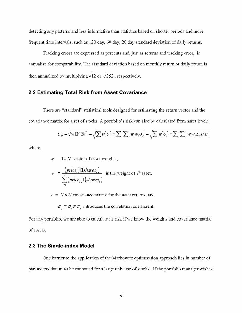
That is, a multi-factor risk model is used to model factor returns and then to estimate the
covariance matrix of factor returns. Specific returns are returns that are unaccounted for by
factors and therefore unique to the security. Specific risks are the variance (or standard
deviation) of specific returns.
The process of building and maintaining a risk model is rather complex. It involves the
following steps:
1. Test, and select a pool of factors. For example price to book and price to cash flow,
among many others, are selected as significant predictors. (See Appendix A.)
2. For the selected factors, formulate the factors and obtain factor exposures. For example,
price to book and price to cash flow are similar and should be grouped as one factor to
describe security’s valuation aspect; call this the factor value. The factor value could be
formulated as value= weight · (price to book) + weight· (price to sales). Price to book
and price to sales each has its own scoring scheme.
12
3. After obtaining factor and factor exposures (scores) for each asset, estimate factor returns
and then estimate the covariance matrix for factor returns.
4. Estimate specific returns and estimate specific risks. Specific returns are uncorrelated
with factor returns, and therefore the covariance of specific return with factors is zero.
Specific returns, on the other hand, are related with the level of market volatility.
This process is diagramed on the following page.
13
Figure 2.1: Building a structured risk model
Model -Fundamental?
-Macroeconomic? -Microeconomic?
Universe Selection -Focus on sector?
-Focus on country?
Factor Selection & Factor formulation
(K factors)
Estimate Factor Estimate Specific
Covariance Matrix ( K K× )
Specific Risk ( 1×N )
Factor Exposures ( N K× )
14
The techniques used for finding and formulating factors vary and can be very involved.
These techniques are beyond the scope of this project. We will focus on risk analysis from the
point of view of a portfolio manager or portfolio construction professional. They are the end-
users of the risk model. From the above diagram, three key sets of inputs are the output of risk
models: the factor covariance matrix, the factor exposures, and the specific risk. Section 3
discusses risk analysis based on the outputs of a multifactor risk model.
2.4 Tracking Error Target Range
Except for the case of index funds, the lowest tracking errors are not always desirable.
Low tracking errors imply a conservative approach towards risk and limit the portfolio’s return
potential. High tracking errors on the other hand expose the portfolio to greater risk. A tracking
error range should be determined before any further risk analysis takes place. After the tracking
error range is set, it needs to be periodically reexamined for appropriateness under the current
market conditions.
Define first the market cross sectional volatility as the standard deviation of all market
security’s returns at one point in time.
[ ]MRStd = MVarR
[ ]
−=
− 2
rrERVar iM
where ir = return of the thi asset in the market. It is important to remember that the market
portfolio is unobservable. Usually a broad index, such as the SP500, is used as proxy and is
referred to as the market.
15
Knowledge of market cross-sectional volatility is helpful in assessing an appropriate
tracking target range. Let’s use the single factor risk model. In a single factor risk model, each
stock’s return is given by:
iMii rr ϖβ +•=
where iMii rr ϖβ +•= ,
=ir stock 'i s return,
iβ = stock 'i s beta,
Mr = market return, and
iϖ = stock 'i s residual return.
Residual returns are assumed to be uncorrelated, and hence
2,( )i j i j MCov r r β β σ= ⋅ ⋅
and so
2222iMii ϖσβσ +=
To see the relation between asset correlation and market volatility, notice that
2
2 2 2 2 2 2( ) ( )i j M
ij
i M i j M j
β β σρ
β σ ϖ β σ ϖ=
+ ⋅ +
Values for stock β ’s are relative stable. Let’s assume β =1, then the above reduces to
22
2
ϖσσρ
+=
M
Mij
Thus, there is a positive correlation between market risk and correlation between assets. Now
let’s take a look at how asset correlation would affect tracking error. In a multifactor model, a
portfolio’s tracking error is given by:
16
2 T TTE x F x w w= ⋅ ⋅ + ⋅∆ ⋅
The first term of the righthand side is the portion of risk explained by the factor model. Keeping
factor exposure constant, with correlation among assets increasing(decrease), factor risk will
increase(decrease).
By the model design, specific risks are the risks unaccounted for by any factors, but the
level of specific risks are affected by the market overall volatility. The specific risks are
estimated by two steps - the first step is a scaling and standardizing of overall market risk and the
second step is a regression analysis of any residual volatility.
Both factor risks and specific risks are affected by market overall volatility, and therefore
the tracking error is not constant. It is important for risk analysis to start with an assessment of
overall market volatility. If there is no significant change in market volatility, then the preset
tracking error range should be upheld, and more focus should be given to risk decomposition.
However, we have examined residual risks of BARRA model and found residual risks
are correlated, which makes the specific risk portion susceptible to asset correlation change also.
17
3. Risk Decomposition Decomposing risk allows portfolio managers to identify and isolate the sources of risk. It
is important primarily for two reasons:
1. It allows the portfolio manager to align the portfolio’s risk with a particular
strategy.
2. It gives additional information regarding the level of real diversification in the
portfolio.
Two portfolios with the same estimated tracking error may have very different risk
characteristics. For example, a portfolio loaded with high beta stocks may have high tracking
errors due to volatility, while another portfolio may tilt towards momentum, which favors recent
winners. Risk characteristics should be in sync with portfolio’s intended management strategy.
A portfolio that is heavily tilted towards one type of factor is very different from a
portfolio with relatively diversified factor risks. Generally, diversification among factors is more
desirable than overly concentrated factor risk. But some factors are by design more volatile
(explaining more variance) than others. For example, in Barra’s USE3 risk model, volatility and
momentum are the volatile factors among common factors, and Gold, Internet, Semi conductors
account for more risk among industry factors.
3.1 Risk Decompositions along Factors
Tracking Error can be decomposed into factor risk and specific risk:
=2TE 2Fσ + 2
Sσ
Here, the specific risk is the weighted sum of the individual asset-specific risks.
∑=
=N
isiiS w
1
222 σσ
18
where iw = thi asset’s active weight, and
siσ = thi asset’s specific risk.
The factor risk (industry factor and common factor) is given by
TF xFx=2σ
where x = Factor Active Exposure ( 1 K× , and K is the number of factors), and
F = Factor Covariance ( K K× matrix).
A portfolio’s exposure to each factor is then computed as
1
N
j ij ii
x Coeff w=
= ⋅∑ for 1, 2,...,j K=
where ijCoeff is the exposure coefficient (score) for the thi security on the thj factor.
Factor exposure measures how a portfolio is exposed to particular factors in the risk
model. This is just the weighted sum of factor scores. Factor exposures are easy to understand
and easy to manage, i.e. to include one or many factor exposure constraints are just adding one or
more linear constraints, while to target factor risk to a range will be harder as they are quadratic
constraints.
Factor Risk (A factor’s contribution to TE)
jjFj xxF=2σ
where 2Fjσ = factor risk attributed to thj factor
x = factor exposure vector (1 K× )
jF = thj factor’s covariance with other factors ( 1K × )
jx = thj factor’s exposure
The marginal contribution to active risk by each factor is then
19
2
j 2MCAR Fj
TEσ
=
Each factor’s contribution to risk is expressed as a percentage of the total risk. It is similar to
common size accounting analysis; using percentages we are able to compare different portfolios
even though they have different levels of tracking error.
3.2 Sources of Factor Exposure
After a factor is identified as a major risk contributor, i.e. a factor accounting for a high
percentage of total risk, further examinations are required:
1. Is the high percentage of risk caused by high exposure or by the variance and
covariance matrix?
2. Is the factor exposure concentrated on a few stocks or it is rather diversified?
Individual security contribution to each risk factor’s exposure can be computed as
ijx = ij iCoeff w⋅
This analysis is simple and useful in isolating the sources of risk exposures. We will see
that in some cases a handful of securities accounts for so much of a factor’s exposure such that if
those are removed, the factor exposure will change dramatically. In other cases, such analysis
exposes data error; sometimes it provides more reasonable calculations for factor scores.
As an example consider the Barra factor momentum. Barra defines momentum as a
combination of relative strength and historical alpha:
a) Relative Strength is defined as cumulative excess return over the past 12 months, using
continuously compounded monthly returns. The excess return is defined as excess return
over the compounded monthly risk-free rate.
20
b) Historical alpha is defined as the excess return from a 60 month regression of the stocks
excess returns on the SP500 excess returns. Again, excess returns are defined as the
excess return over the risk-free rate.
Let us use MRVL as example: MRVL’s IPO price was at $15 but the first trade was $50.
In essence, MRVL has a positive return over the past three years but a meaningful loss (-70%) if
calculated from when investors could actually buy the stock. Thus, momentum scores based on
IPO price for cases like MRVL can be misleading. There are might be plenty of cases similar to
MRVL that IPOed in 1999/2000. And such a problem will be easy to spot when we analyze
factor exposure by security contribution.
Taking action to adjust factor coefficients for certain securities, (which can be costly), or
not taking action but being able to readjusting tolerance to certain risk factors, either way, both
are direct benefits from understanding the source of factor risk.
3.3 A Security’s contribution to One Risk Factor’s Factor Risk
It is useful to focus more closely on how an individual security contributes to a specific
risk factor. We have
2ij j ij ix F Coeff wσ = ⋅ ⋅ ⋅ ( thi security’s risk contribution to thj factor’s risk),
as well as
2 2
1
K
i ijj
σ σ=
=∑ ( thi security’s risk contribution to factor risk).
This shows that one asset’s contribution to one risk factor depends on
1. the security’s active weight,
2. the security’s exposure coefficient for that factor, and
21
3. the factor’s relative “significance” (active exposure times covariance with other
factors)
However, a security also contributes to the factor exposure, making it difficult to assign and
interpret. .
3.4 Risk Decompositions across Securities
Each security’s contribution to tracking error can be expressed as the sum of security
risks:
=2TE 2
1
N
ii
σ=∑
where 2iσ = the thi security’s contribution to TE
N = the number of assets in the portfolio.
It is important to note that 2iσ is a security’s contribution to the portfolio’s tracking error and
has to be put into the context of the portfolio being analyzed. This is not the intrinsic risk or
variance of a security that is measured based the securities historical movements alone, rather it
is calculated given a security’s active weight in the portfolio, its factor risk and specific risk in
the portfolio.
Each individual security’s contribution to tracking error can be expressed as
2 2 2
1
K
i j ij i i sij
x F Coeff w wσ σ=
= ⋅ ⋅ ⋅ + ⋅∑
where
ijCoeff = the exposure coefficient for the thi security on the thj factor
One asset’s contribution to TE is the sum of the asset’s
22
1) factor risk contribution, and
2) specific risk contribution.
Thus, the marginal contribution to active risk (MCAR) can be calculated as:
2
2MCAR ii TE
σ= .
23
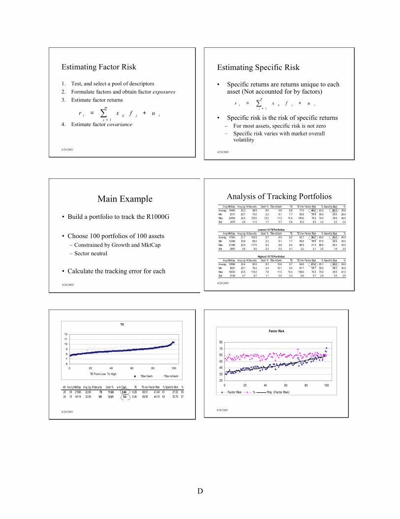
4. Portfolio Construction and Risk Analysis Based on a Paper Portfolio
This chapter discusses an example based on the Barra USE3 Risk model used to construct
an index fund that tracks the R1000G. The Russell 1000G is a large-cap index developed and
maintained by Russell, an investment services firm. The index measures the performance of the
largest 1,000 U.S. incorporated companies.
The Russell 1000G measures the performance of those Russell 1000 companies with
higher price-to-book ratios and higher forecasted growth values.
4.1 Tracking the Russell 1000G
Indexed funds are growing popular due to several factors:
- Low cost. An indexed mutual fund charges around 0.3% of asset, whereas an
actively managed mutual fund normally costs around 1.3% of asset to investors.
- The assumption of market efficiency.
- A proliferation of quantitative risk models and portfolio construction tools.
The primary goal of indexing is to track the target portfolio as closely as possible. For
this exercise, our goal is to choose a portfolio with the lowest tracking error. There are also other
constraints set for this index fund:
- no more than 100 assets
- no more than 5% cash holding
- single asset will exceed 2.5% of weight of the portfolio
- sector neutral
Initial construction as of date 2001/12/06.
24
Step 1: Generate 100 names
On the portfolio formation date, R1000G had around 550 assets. To randomly choose 100
from 550 assets, we need to generate a set of random number with probability of
0.1818(=100/550), that is, the selection of an asset can be represented as:
1818.0)1( ==XP
where X is a 0, 1 variable indicating in or out of sample.
We also wish to mimic the distribution of growth and market capitalization in the
R1000G. Growth and capitalization are basic characteristics of a portfolio, and are widely used
to determine the style of a portfolio. Assuming growth and market cap are independent, the joint
probability can be represented as:
)1( =XP = )1( =gXP )1( =mXP = 0.1818
and
)1( =gXP = )1( =mXP = 0.4264
where the subscripts g, and m indicate whether the indicator is for growth or market cap.
In the algorithm, first rank each of R1000 constituents by growth and market cap, and
then each security takes a uniform random number with probability of 0.4264.
Step 2: Assign weight of holdings
To mimic sector exposure of R1000G,
jj
n
ii WIw
j
=∑=1
mjni j ..1,...1 ==
where =iw the weight of a security in the portfolio
jn = the number of securities in the portfolio that belong to sector j
25
=jW the sector weight in the benchmark
In this step, jW is determined by the benchmark; jn is determined after the names are
chosen. If we set jwIw ji
−= , that is, a security’s weight equals the average weight of assets in
the sector, we have
jwIw ji
−= = jj nW /
The final adjustment is if any single security holding exceeds 2.5%, set the holding to be
2.5%. The choice of 2.5% is arbitrary and in fact 2.5% is rather large in a diversified portfolio,
some investors may have higher or lower tolerance.
Step 3: Calculate the estimated tracking error for the synthesized portfolios
The tracking errors and other information, such as portfolio’s average market cap,
average long term growth rate, are calculated as a basis for choosing the initial portfolio.
4.1 A Complete Step-By-Step Risk Analysis
Analysis of the 100 portfolios begins by reviewing the composition of factor risk and specific
• Risk analysis based on Risk Models– Benchmarks, Tracking Error– Factor Models and Factor Decomposition
• Example in Detail– Tracking the Russell 1000 Growth
4/28/2003
Background: Active versus Passive Management• Measure return relative to a benchmark.
– Passive: believe the market is efficient, and the goal is to match the benchmark
– Active: believe that active stock selection will outperform market, and the goal is to beat the benchmark
• Measure total risk relative to the same benchmark– Passive: maintain a tight risk target range and try to match
benchmark risk as closely as possible– Active: manage portfolio risk characteristics to be in line with
active stock selection strategy, and target risk within a specific lower and upper bounds
4/28/2003
Classical Modern Portfolio Theory
• Markowitz: Efficient Frontier
• Maximize Utility:
M
BA
Capital Market Line
Efficient Frontier
Eσ
ERr
σ
X
Y
2PPRU λσ−=
4/28/2003
Some Notation• Universe of stocks:
• Expected returns:
• Covariance matrix:
• Portfolio returns:
• Portfolio risk:
1,2,...,i N=
( )i iE Rµ =
( ) ( )ij i i j jE R Rσ µ µ = − ⋅ −
Vwwww Ti j ijjiP ==∑ ∑ σσ 2
∑= iiP uwR
C
4/28/2003
Portfolio Construction And Risk Analysis
OptimizerMaximizes
Utility
Riskσ
Constraints Bounds
Exp. Returnsα
PortfolioUniverseBenchmark
OptimallyWeightedPortfolio
4/28/2003
Estimating Risk
• Problems with asset covariance matrix – Parameter estimation is hard– Provides little workable information
• Advantages of risk models– Reduce parameter space– Provide ways to manage risk through exposures– Provides ways to attribute risk to factors by percent of
total risk
4/28/2003
Estimating Portfolio’s Risk
• Tracking ErrorTracking Error is the standard deviation of portfolio's active return
-Historical Realization Based on 36-monthly returns, 120, 60, 20- daily returns
-Estimated Based On Assets (Modern Portfolio Theory)
[ ]Bpp RRStd −≡σ
2 2 2 2TP i i i j ij i i i j ij i ji j i j
w V w w ww w wwσ σ σ σ ρσσ= ⋅ ⋅ = + = +∑ ∑∑ ∑ ∑∑
4/28/2003
Estimating Portfolio’s Risk
Estimated Based On Factors (Risk Models)
wherex: M by 1 Factor Exposure VectorF: M by M Factor Covariance Matrix