Posterior Distribution of Nondifferentiable Functions

Toru KitagawaJose-Luis Montiel-Olea Jonathan Payne

The Institute for Fiscal Studies Department of Economics, UCL

cemmap working paper CWP20/16

POSTERIOR DISTRIBUTION OF NONDIFFERENTIABLE FUNCTIONS.1

Toru Kitagawa2, José-Luis Montiel-Olea3 and Jonathan Payne4

This paper examines the asymptotic behavior of the posterior distributionof a possibly nondifferentiable function g(θ), where θ is a finite dimensionalparameter. The main assumption is that the distribution of the maximum like-lihood estimator θ̂n, its bootstrap approximation, and the Bayesian posteriorfor θ all agree asymptotically.

It is shown that whenever g is Lipschitz, though not necessarily differen-tiable, the posterior distribution of g(θ) and the bootstrap distribution ofg(θ̂n) coincide asymptotically. One implication is that Bayesians can interpretbootstrap inference for g(θ) as approximately valid posterior inference in alarge sample. Another implication—built on known results about bootstrapinconsistency—is that the posterior distribution of g(θ) does not coincide withthe asymptotic distribution of g(θ̂n) at points of nondifferentiability. Conse-quently, frequentists cannot presume that credible sets for a nondifferentiableparameter g(θ) can be interpreted as approximately valid confidence sets (evenwhen this relation holds true for θ).

Keywords: Bootstrap, Bernstein von-Mises Theorem, Directional Differ-entiability, Posterior Inference.

1. INTRODUCTION

This paper studies the posterior distribution of a real-valued function g(θ), whereθ is a parameter of finite dimension. We focus on a class of models where the trans-formation g(θ) is Lipschitz continuous but possibly nondifferentiable. Some stylizedexamples are:

|θ|,max{0, θ},max{θ1, θ2}.

Parameters of the type considered in this paper arise in a wide range of applicationsin economics and statistics. Some examples are the welfare level attained by an op-timal treatment assignment rule in the treatment choice problem (Manski (2004));a trading strategy in an asset market (Jha and Wolak (2015)); the regression func-tion in a regression kink model with an unknown threshold (Hansen (2015)); the

1We would like to thank Gary Chamberlain, Tim Cogley and Quang Vuong for detailed commentsand suggestions on a earlier draft of this paper. All errors remain our own. Financial support fromthe ESRC through the ESRC Centre for Microdata Methods and Practice (CeMMAP) (grantnumber RES-589-28-0001) is gratefully acknowledged. This draft: May 6, 2016.

2University College London, Department of Economics. E-mail: t.kitagawa@ucl.ac.uk.3New York University, Department of Economics. E-mail: montiel.olea@nyu.edu.4New York University, Department of Economics. E-mail: jep459@nyu.edu.

1

2 KMP

eigenvalues of a random symmetric matrix (Eaton and Tyler (1991)); and the valuefunction of stochastic mathematical programs (Shapiro (1991)). The lower and up-per bound of the identified set in a partially identified model are also examples ofparameters that fall within the framework of this paper.1

The potential nondifferentiability of g(·) poses different challenges to frequentistinference. For example, different forms of the bootstrap lose their consistency when-ever differentiability is compromised; see Dümbgen (1993), Andrews (2000) andthe recent characterization of bootstrap failure in Fang and Santos (2015). To ourknowledge, the literature has not yet explored how the Bayesian posterior of g(θ)relates to the distribution of the (plug-in) maximum likelihood (ML) estimator andits bootstrap distribution when g is allowed to be nondifferentible.This paper studies these relations in large samples. The main assumptions are

that: (i) the ML estimator for θ, denoted by θ̂n, is√n-asymptotically normal,

(ii) the bootstrap consistently estimates the asymptotic distribution of θ̂n and (iii)the Bernstein-von Mises Theorem holds for θ (DasGupta (2008), p. 291); i.e., theBayesian posterior distribution of θ coincides with the asymptotic distribution ofθ̂n.This paper shows that—after appropriate centering and scaling—the posterior

distribution of g(θ) and the bootstrap distribution of g(θ̂n) are asymptotically equiv-alent. This means that the bootstrap distribution of g(θ̂n) contains, in large samples,the same information as the posterior distribution for g(θ).2

This result provides two useful insights. First, Bayesians can interpret bootstrap-based inference for g(θ) as approximately valid posterior inference in a large sample.Thus, Bayesians can use bootstrap draws to conduct approximate posterior inferencefor g(θ) when computing θ̂n is simpler than Markov Chain Monte Carlo (MCMC)sampling.Second, combined with the known results on the failure of bootstrap inference,

we show that the Bernstein-von Mises Theorem for g(θ) will not hold even undermild departures from differentiability. In particular, the posterior distribution of g(θ)

1For example, treatment effect bounds (Manski (1990), Balke and Pearl (1997)); bounds in auc-tion models (Haile and Tamer (2003)), and bounds for impulse-response functions (Giacomini andKitagawa (2015), Gafarov, Meier, and Montiel Olea (2015)) and forecast-error variance decompo-sitions (Faust (1998)) in structural vector autoregressions.

2Other results in the literature concerning the relations between bootstrap and posterior inferencehave focused on the Bayesian interpretation of the bootstrap in finite samples, for example Rubin(1981), or on how the parametric bootstrap output can be used for efficient computation of theposterior, for example Efron (2012).

3

will not coincide with the asymptotic distribution of g(θ̂n) whenever g(·) only hasdirectional derivatives as in the pioneering work of Hirano and Porter (2012). In fact,it is shown that whenever directional differentiability causes a bootstrap confidenceset to cover g(θ) less often than desired, a credible set based on the quantiles of theposterior will have distorted frequentist coverage as well.The rest of this paper is organized as follows. Section 2 presents a formal statement

of the main results. Section 3 presents an illustrative example: the absolute valuetransformation. Section 4 concludes. All the proofs are collected in the Appendix.

2. MAIN RESULTS

Let Xn = {X1, . . . Xn} be a sample of i.i.d. data from the parametric modelf(xi | θ), with θ ∈ Θ ⊆ Rp. Let θ̂n denote the ML estimator of θ and let θ0 denotethe true parameter of the model. Consider the following assumptions:

Assumption 1 The function g : Rp → R is Lipschitz continuous with constantc. That is;

|g(x)− g(y)| ≤ c||x− y|| ∀ x, y ∈ Rp.

Assumption 1 implies—by means of the well-known Rademacher’s Theorem (Evansand Gariepy (2015), p. 81)—that g is differentiable almost everywhere in Rp. Thus,the functions considered in this paper allow only for mild departures from differen-tiability.3

Assumption 2 The sequence Zn ≡√n(θ̂n − θ0) d→ Z ∼ N(0, I−1(θ0)), where

I−1(θ0) is the inverse of Fisher’s Information matrix evaluated at θ0.

Assumption 2 is high-level, but there are well-known conditions on the statisticalmodel f(x; θ) under which Assumption 2 obtains (see, for example, Newey andMcFadden (1994) p. 2146).In order to state the next assumption, we introduce additional notation. Define

the set:

BL(1) ≡{f : Rp → R| sup

a∈Rk|f(a)| ≤ 1 and |f(a1)−f(a2)| ≤ ||a1−a2|| ∀a1, a2

}.

3Moreover, we assume that g is defined everywhere in Rp which rules out examples such as theratio of means θ1/θ2, θ2 6= 0 discussed in Fieller (1954) and weakly identified Instrumental Variablesmodels.

4 KMP

Let φ∗n and ψ∗n be random variables whose distribution depends on the data Xn.The Bounded Lipschitz distance between the distributions induced by φ∗n and ψ∗n

(conditional on the data Xn) is defined as:

β(φ∗n, ψ∗n; Xn) ≡ supf∈BL(1)

∣∣∣E[f(φ∗n)|Xn]− E[f(ψ∗n)|Xn]∣∣∣.

The random variables φ∗n and ψ∗n are said to converge in Bounded Lipschitz dis-tance in probability if β(φ∗n, ψ∗n; Xn) p→ 0 as n→∞.4

Let θP∗n denote the random variable with law equal to the posterior distributionof θ in a sample of size n. Let θB∗n denote the random variable with law equal tothe bootstrap distribution of the Maximum Likelihood estimator of θ in a sampleof size n.

Remark 1 In a parametric model for i.i.d. data there are different ways of boot-strapping the distribution of θ̂n. One possibility is a parametric bootstrap, whichconsists in generating draws (x1, . . . xn) from the model f(xi; θ̂n) followed by an eval-uation of the ML estimator for each draw (Van der Vaart (2000) p. 328). Anotherpossibility is the standard mutinomial bootstrap, which generates draws (x1, . . . xn)from its empirical distribution. We do not take a stand on the specific bootstrapprocedure used by the researcher as long as it is consistent. This is formalized in thefollowing assumption.

Assumption 3 The centered and scaled random variables:

ZP∗n ≡√n(θP∗n − θ̂n) and ZB∗n ≡

√n(θB∗n − θ̂n),

converge (in the Bounded Lipschitz distance in probability) to the asymptotic dis-tribution of the ML estimator Z ∼ N(0, I−1(θ0)), which is independent of the data.That is,

β(ZP∗n , Z; Xn) p→ 0

andβ(ZB∗n , Z; Xn) p→ 0.

Sufficient conditions for Assumption 3 to hold are the consistency of the boot-4For a more detailed treatment of the bounded lipschitz metric over probability measures see the

‘β’ metric defined in p. 394 of Dudley (2002).

5

strap for the distribution of θ̂n (Horowitz (2001), Van der Vaart and Wellner (1996)Chapter 3.6, Van der Vaart (2000) p. 340) and the Bernstein-von Mises Theoremfor θ.5

The following theorem shows that under the first three assumptions, the Bayesianposterior for g(θ) and the frequentist bootstrap distribution of g(θ̂n) converge (afterappropriate centering and scaling). Note that for any measurable function g(·), be itdifferentiable or not, the posterior distribution of g(θ) can be defined as the imagemeasure induced by the distribution of θP∗n under the mapping g(·).

Theorem 1 Suppose that Assumptions 1, 2 and 3 hold. Then,

β(√n(g(θP∗n )− g(θ̂n)),

√n(g(θB∗n )− g(θ̂n)); Xn) p→ 0.

That is, after centering and scaling, the posterior distribution g(θ) and the bootstrapdistribution of g(θ̂n) are asymptotically close to each other in terms of the BoundedLipschitz metric in probability.

Proof: See Appendix A.1. Q.E.D.

The intuition behind Theorem 1 is the following. The centered and scaled posteriorand bootstrap distributions can be written as:

√n(g(θP∗n )− g(θ̂n)) =

√n(g(θ0 + ZP∗n /

√n+ Zn/

√n)− g(θ̂n)),

√n(g(θB∗n )− g(θ̂n)) =

√n(g(θ0 + ZB∗n /

√n+ Zn/

√n)− g(θ̂n))

Because ZP∗n and ZB∗n both converge, by assumption, to a common limit Z and g isLipschitz, the centered and scaled posterior and bootstrap distributions (conditionalon the data) can both be well approximated by:

√n(g(θ0 + Z/

√n+ Zn/

√n)− g(θ̂n))

and so the desired convergence result obtains. Theorem 1 does not rely on thenormality assumption, but we impose this condition for the sake of exposition.

5Note that the Berstein-von Mises Theorem is oftentimes stated in terms of almost-sure con-vergence of the posterior density to a normal density (DasGupta (2008) p. 291). This mode ofconvergence (total variation metric) implies convergence in the bounded Lipschitz metric in proba-bility. In this paper, all the results concerning the asymptotic behavior of the posterior are presentedin terms of the Bounded-Lipschitz metric. This facilitates comparisons with the boostrap.

6 KMP

If the additional assumption is made that the function g is directionally differ-entiable, a common approximation to the distribution of the bootstrap and theposterior can be characterized explictly.

Assumption 4 There exists a continuous function g′θ0 : Rp → R such that forany compact set K ⊆ Rp and any sequence of positive numbers tn → 0:

suph∈K

∣∣∣t−1n (g(θ0 + tnh)− g(θ0))− g′θ0(h)

∣∣∣→ 0,

The continuous, not necessarily linear, function g′θ(·) will be referred to as the(Hadamard) directional derivative of g at θ0.6

Remark 2 Note that the notion of Hadamard directional derivative is, in principle,stronger than the notion of one-sided directional derivative (or Gateaux directionalderivative) used in Hirano and Porter (2012). The former requires the approximationto be uniform over directions h that belong to a compact set, whereas the latteris pointwise in h. However, when g is Lipschitz it can be shown that one-sideddirectional differentiability implies Hadamard directional differentiability and so,for the environment described in this paper, the concepts are equivalent. We stateAssumption 4 using the Hadamard formulation (as that is the property required inthe proofs), but we remind the reader that in a Lipschitz environment it is sufficientto show one-sided directional differentiability to verify Assumption 4.

Corollary 1 Let θ0 denote the parameter that generated the data. Under As-sumptions 1, 2, 3, and 4:

β(√n(g(θP∗n )− g(θ̂n)), g′θ0(Z + Zn)− g′θ0(Zn) ; Xn) p→ 0,

where Z ∼ N(0, I−1(θ0)) and Zn =√n(θ̂n − θ0).

Proof: See Appendix A.2. Q.E.D.

6Equivalently, one could say there is a continuous function g′θ : Rk → R such that for anyconverging sequence hn → h:∣∣∣∣√n(g(θ0 + hn√

n

)− g(θ0)

)− g′θ0 (hn)

∣∣∣∣→ 0.

See p. 479 in Shapiro (1990).

7

The distribution g′θ0(Z + Zn) − g′θ0(Zn) (which still depends on the sample size)provides a large-sample approximation to the distribution of g(θP∗n ). Our resultshows that, in large samples, after centering aroung g(θ̂n), the data will only affectthe posterior distribution through Zn =

√n(θ̂n − θ0).

The approximating distribution has appeared in the literature before, see Propo-sition 1 in Dümbgen (1993) and equation A.41 in Theorem A.1 in Fang and Santos(2015). Thus, verifying the assumptions for any of these papers in combination withour Theorem 1 would suffice to establish our Corollary 1. In order to keep the ex-position self-contained, we decided to present a simpler derivation of this law usingour own specific assumptions.

The intuition behind our proof is as follows. When g is directionally differentiablethe approximation used to establish Theorem 1:

√n(g(θ0 + Z/

√n+ Zn/

√n)− g(θ̂n)) =

√n(g(θ0 + Z/

√n+ Zn/

√n)− g(θ0))

−√n(g(θ0 + Zn/

√n)− g(θ0)),

can be further refined to:g′θ0(Z + Zn)− g′θ0(Zn).

This follows from the fact that

√n(g(θ0 + Z/

√n+ Zn/

√n)− g(θ0))

is a perturbation around θ0 in the random direction (Z + Zn) and is well approxi-mated by g′θ0(Z + Zn). Likewise,

√n(g(θ0 + Zn/

√n)− g(θ0))

is a perturbation around θ0 in direction Zn and it is well approximated by g′θ0(Zn).

Remark 3 Note that if g′θ0 is linear (which is the case if g is fully differentiable),then

√n(g(θP∗n )− g(θ̂n)) converges to:

g′θ0(Z + Zn)− g′θ0(Zn) = g′θ0(Z) ∼ N (0, (g′θ0)TI−1(θ0)(g′θ0)),

where (g′θ0)T denotes the transpose of the gradient vector g′θ0 . This is the samelimit as one would get from applying the delta method to g(θ̂n). Thus, under full

8 KMP

differentiability, the posterior distribution of g(θ) can be approximated as:

g(θP∗n ) ≈ g(θ̂n) + 1√ng′θ0(Z).

Moreover, this distribution coincides with the asymptotic distribution of the plug-inestimator g(θ̂n). The obvious remark is that full differentiability is sufficient for aBernstein-von Mises Theorem to hold for g(θP∗n ).

If g′θ0 is nonlinear the limiting distribution of√n(g(θP∗n ) − g(θ̂n)) becomes a

nonlinear transformation of Z. This nonlinear transformation need not be Gaus-sian, and need not be centered at zero. Moreover, the nonlinear transformationg′θ0(Z+Zn)−g′θ0(Zn) is different from the asymptotic distribution of the plug-in es-timator g(θ̂n) which is given by g′θ0(Z).7 Informally, one can say that for directionallydifferentiable functions:

g(θP∗n ) ≈ g(θ̂n) + 1√n

(g′θ0(Z + Zn)− g′θ0(Zn)), where Zn =√n(θ̂n − θ0).

Failure of Bootstrap Inference: Theorem 1 established the large-sampleequivalence between the bootstrap distribution of g(θ̂n) and the posterior distri-bution of g(θ). We now use this Theorem to make a concrete connection betweenthe coverage of bootstrap-based confidence sets and the coverage of Bayesian credi-ble sets based on the quantiles of the posterior.Neither the results of Dümbgen (1993) nor those of Fang and Santos (2015) offer

a concrete chacterization of the asymptotic coverage of bootstrap-based confidencesets. Despite the bootstrap inconsistency established in these papers, it is still pos-sible that the bootstrap confidence sets have correct asymptotic coverage.In this section we will not insist in characterizing the asymptotic coverage of

bootstrap and/or posterior inference. Instead, we start by assuming that a nominal(1 − α) bootstrap confidence set fails to cover g(θ) at a point of directional differ-entiability. Then, we show that a (1− α − ε) credible set based on the quantiles ofthe posterior distribution of g(θ) will also fail to cover g(θ) for any ε > 0.8

7This follows from an application of the delta-method for directionally differentiable functions inShapiro (1991)) or from Proposition 1 in Dümbgen (1993).

8The adjustment factor ε is introduced because the the quantiles of both the bootstrap and theposterior remain random even in large samples.

This result is not a direct corollary of Theorem 1 as there is some extra work needed to relatethe quantiles of the bootstrap distribution of g(θ̂n) and the quantiles of the posterior of g(θ).

9

Set-up: Let qBα (Xn) be defined as:

qBα (Xn) ≡ infc{c ∈ R | PB∗(g(θB∗n ) ≤ c |Xn) ≥ α}.

The quantile based on the posterior distribution qPα (Xn) is defined analogously.A nominal (1−α)% two-sided confidence set for g(θ) based on the bootstrap dis-

tribution g(θB∗n ) can be defined as follows:

CSBn (1− α) ≡[qBα/2(Xn) , qB1−α/2(Xn)

].(2.1)

This is a typical confidence set based on the percentile method of Efron, p. 327 inVan der Vaart (2000).

Definition We say that the nominal (1− α)% bootstrap confidence set fails tocover the parameter g(θ) at θ by at least dα% (dα > 0) if:

(2.2) lim supn→∞

Pθ(g(θ) ∈ CSBn (1− α)

)≤ 1− α− dα,

where Pθ refers to the distribution of Xi under parameter θ.

Let Fθ(y|Zn) denote the c.d.f. of the random variable Y ≡ g′θ(Z + Zn) condi-tional on Zn. In order to relate our weak convergence results to the behavior of thequantiles, we assume that at the point θ where the bootstrap fails the followingassumption is satisfied:

Assumption 5 The c.d.f. Fθ(y|Zn) is Lipschitz continuous with a constant kthat does not depend on Zn.9

Assumption 5 suffices to relate the coverage of a confidence set for g(θ) based onthe quantiles of the posterior of g(θ) with the coverage of a bootstrap confidenceset.10 We establish this connection as another Corollary to Theorem 1.

9A sufficient condition for this result to hold is that the density hθ(y|Zn) admits an upper boundindependent of Zn. This will be the case in the illustrative example we consider.

10Assumption 5 could be relaxed. Appendix A.3 presents a high-level condition implied by As-sumption 5 that requires the existence of a value ζ such that, for all c ∈ R, the probability thatg′θ(Z + Zn) − g′θ(Zn) is in the interval [c − ζ, c + ζ] can be made arbitrarily small (for most datarealizations).

10 KMP

Corollary 2 Suppose that the nominal (1 − α)% bootstrap confidence set failsto cover g(θ) at θ by at least dα%. If Assumptions 1 to 5 hold then for any ε > 0 :

lim supn→∞

Pθ(g(θ) ∈

[qP(α+ε)/2(Xn) , qP1−(α+ε)/2(Xn)

])≤ 1− α− dα.

Thus, for any 0 < ε < d, the nominal (1−α−ε)% credible set based on the quantilesof the posterior fails to cover g(θ) at θ by at least (dα − ε)%.

Proof: See Appendix A.3. Q.E.D.

The intuition behind the theorem is the following. For convenience, let θ∗n denoteeither the bootstrap or posterior random variable and let c∗β(Xn) denote the β-critical value of g(θ∗n) defined by:

c∗β(Xn) ≡ infc{c ∈ R | P∗(

√n(g(θ∗n)− g(θ̂n)) ≤ c |Xn) ≥ β}.

We show that c∗β(Xn) is asymptotically close to the β-quantile of g′θ(Z+Zn)−g′θ(Zn),denoted by cβ(Zn). More precisely, we show that for arbitrarily small 0 < ε < β andδ > 0, the probability that c∗β(Xn) ∈ [cβ−ε/2(Zn), cβ+ε/2(Zn)] is greater than 1 − δfor sufficiently large n.Because under Assumptions 1 to 5 the critical values of both the bootstrap and

posterior distributions are asymptotically close to the quantiles of g′θ(Z + Zn) −g′θ(Zn), we can show that for a fixed ε > 0 and sufficiently large n:

Pθ(g(θ) ∈ CSBn (1− α)

)= Pθ

(g(θ) ∈

[qP(α+ε)/2(Xn) , qP1−(α+ε)/2(Xn)

])− δ.

It follows that when the (1−α)%–bootstrap confidence set fails to cover the param-eter g(θ) at θ, then so must the (1− α− ε)%–credible set.11

11It immediately follows that the reverse also applies. If the (1− α)%–credible set fails to coverthe parameter g(θ) at θ, then so must the (1 − α − ε)%–bootstrap confidence set. Note that ourapproximation holds for any fixed ε, but we cannot guarantee that our approximation holds if wetake the limit.

11

3. ILLUSTRATION OF MAIN RESULTS FOR |θ|

The main result of this paper, Theorem 1, can be illustrated in the followingsimple environment. Let Xn = (X1, . . . Xn) be an i.i.d. sample of size n from thestatistical model:

Xi ∼ N (θ, 1).

Consider the following family of priors for θ:

θ ∼ N(0, (1/λ2)),

where the precision parameter satisfies λ2 > 0. The transformation of interest is theabsolute value function:

g(θ) = |θ|.

It is first shown that when θ0 = 0 this environment satisfies Assumptions 1 to 5.Then, the bootstrap and posterior distributions for g(θ) are explicitly computed andcompared.

Relation to main assumptions: The tranformation g is Lipschitz continuousand differentiable everywhere, except at θ0 = 0. At this particular point in theparameter space, g has directional derivative g′0(h) = |h|. Thus, Assumptions 1 andAssumption 4 are both satisfied.

The Maximum Likelihood estimator is given by θ̂n = (1/n)∑ni=1Xi and so

√n(θ̂n−

θ) ∼ Z ∼ N (0, 1). This means that Assumption 2 is satisfied.

This environment is analytically tractible so the distributions of θP∗n and θB∗n canbe computed explicitly. The posterior distribution for θ is given by:

θP∗n |Xn ∼ N( n

n+ λ2 θ̂n,1

n+ λ2

),

which implies that:

√n(θP∗n − θ̂n)|Xn ∼ N

( λ2

n+ λ2√nθ̂n,

n

n+ λ2

).

Consequently,β(√

n(θP∗n − θ̂n) , N (0, 1);Xn)

p→ 0.

12 KMP

This implies that under, θ0 = 0, the first part of Assumption 3 holds.12

Second, consider a parametric bootstrap for the sample mean, θ̂n. We decidedto focus on the parametric bootstrap to keep the exposition as simple as possible.The parametric bootsrap is implemented by generating a large number of draws(xj1, . . . , xjn), j = 1, . . . , J from the model

xji ∼ N (θ̂n, 1), i = 1, . . . n,

recomputing the ML estimator for each of the draws. This implies that the boostrapdistribution of θ̂n is given by:

θB∗n ∼ N (θ̂n, 1/n),

and so, for the parametric bootstrap it is straightforward to see that:

β(√

n(θB∗n − θ̂n) , N (0, 1);Xn)

= 0.

This means that the second part of Assumption 3 holds.

Finally, in this example the p.d.f. of Y ≡ g′0(Z+Zn) = |Z+Zn| is that of a foldednormal:

h0(y|Zn) = 1√2π

exp(− 1

2(y − Zn)2)

+ 1√2π

exp(− 1

2(y + Zn)2),

this expression follows by direct computation or by replacing cosh(x) in equa-tion 29.41 in p. 453 in Johnson, Kotz, and Balakrishnan (1995) by (1/2)(exp(x) +exp(−x)). Note that:

h0(y|Zn) ≤√

2π,

12The last equation follows from the fact that for two Gaussian real-valued random variablesX ∼ N (µ1, σ

21) and Y ∼ N (µ2, σ

22) we have that:∣∣∣E[f(X)]− E[f(Y )]

∣∣∣ ≤√ 2π

∣∣∣σ21 − σ2

2

∣∣∣+∣∣∣µ1 − µ2

∣∣∣.Therefore:

β(√

n(θP∗n − θ̂n) , N (0, 1);Xn)≤√

2π

∣∣∣ n

n+ λ2 − 1∣∣∣+∣∣∣ λ2

n+ λ2

√nθ̂n

∣∣∣.

13

which implies that Assumption 5 holds. To see this, take y1 > y2. Note that:

Fθ(y1|Zn)− Fθ(y2|Zn) =∫ y1

y2h(y|Zn)dy ≤ (y1 − y2)

√2π.

An analogous argument for the case in which y1 ≤ y2 implies that Assumption 5 isverified.

Asymptotic Behavior of Posterior Inference for g(θ) = |θ|: Since As-sumptions 1 to 4 are satisfied, Theorem 1 and its Corollary hold.In this example the posterior distribution of g(θ∗P )|Xn is given by:

∣∣∣ 1√n+ λ2

Z∗ + n

n+ λ2 θ̂n∣∣∣, Z∗ ∼ N (0, 1)

and therefore√n(g(θ∗P )− g(θ̂n) can be written as :

∣∣∣ √n√

n+ λ2Z∗ + n

n+ λ2√nθ̂n

∣∣∣− ∣∣∣√nθ̂n∣∣∣, Z∗ ∼ N (0, 1).(3.1)

Theorem 1 and its Corollary show that when θ0 = 0 and n is large enough, thisexpression can be approximated in the Bounded Lipschitz metric in probability by:∣∣∣Z + Zn

∣∣∣− ∣∣∣Zn∣∣∣ =∣∣∣Z +

√nθ̂n

∣∣∣− ∣∣∣√nθ̂n∣∣∣, Z ∼ N (0, 1).(3.2)

Observe that at θ0 = 0 the sampling distribution of the plug-in ML estimator for|θ| is given by:

√n(|θ̂n| − |θ0|) ∼ |Z|.

Thus, the approximate distribution of the posterior differs from the asymptotic dis-tribution of the plug-in ML estimator and the typical Guassian approximation forthe posterior will not be appropriate.

Asymptotic Behavior of Parametric Bootstrap Inference for g(θ) = |θ|:The parametric bootstrap distribution of |θ̂n|, centered and scaled, is simply givenby: ∣∣∣Z +

√nθ̂n

∣∣∣− |√nθ̂n|, Z ∼ N(0, 1),

which implies that posterior distribution of |θ| and the bootstrap distribution of |θ̂n|

14 KMP

are asymptotically equivalent.

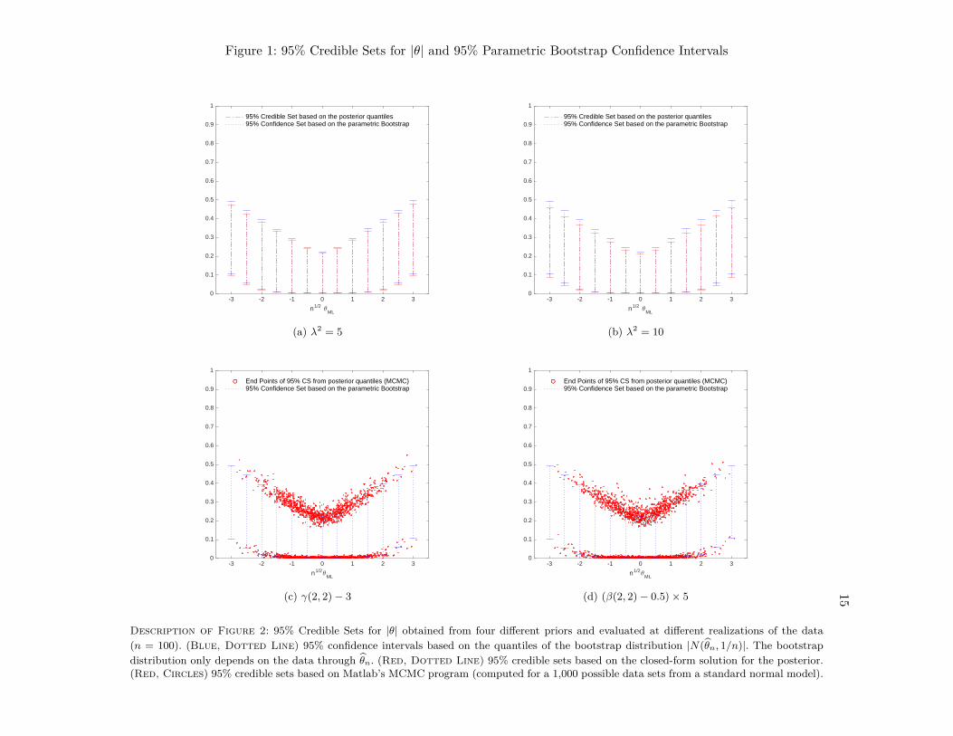
Graphical interpretation of Theorem 1: One way to illustrate Theorem 1is to compute the 95% credible sets for |θ| when θ0 = 0 using the quantiles of theposterior. We can then compare the 95% credible sets to the 95% confidence setsfrom the bootstrap distribution. Note that in establishing Corollary 2 we have shownthat this relation is indeed implied by Theorem 1.Observe from (3.2) that the approximation to the centered and scaled posterior

and bootstrap distributions depends on the data via√nθ̂n. Thus, in Figure 2 we

report the 95% credible and confidence sets for data realisations√nθ̂n ∈ [−3, 3]. In

all four plots the bootstrap confidence sets are computed using the parametric boot-strap. Posterior credible sets are presented for four different priors for θ: N (0, 1/5),N (0, 1/10), γ(2, 2)− 3 and (β(2, 2)− 0.5)× 5. The posterior for the first two priorsis obtained using the expression in (3.1), while the posterior for the last two priorsis obtained using a the Metropolis-Hastings algorithm (Geweke (2005), p. 122).

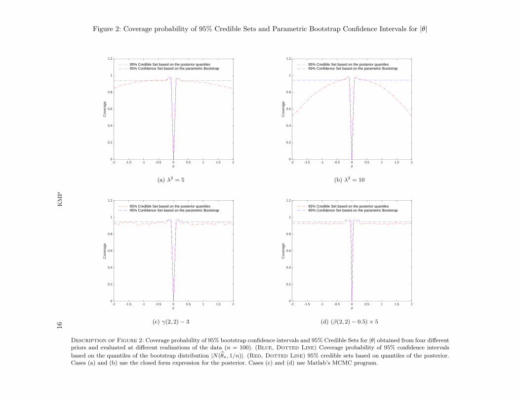
Coverage of Credible Sets: In this example, the two-sided confidence set basedon the quantiles of the bootstrap distribution of |θ̂n| fails to cover |θ| when θ = 0.Corollary 2 showed that the two-sided credible sets based on the quantiles of theposterior should exhibit the same problem. This is illustrated in Figure 2. Thus, afrequentist cannot presume that a credible set for |θ| based on the quantiles of theposterior will deliver a desired level of coverage.As Liu, Gelman, and Zheng (2013) observe, although it is common to report

credible sets based on the α/2 and 1 − α/2 quantiles of the posterior, a Bayesianmight find these credible sets unsatisfactory. In this problem, it is perhaps morenatural to consider one-sided credible sets or Highest Posterior Density sets. In theonline Appendix B we consider an alternative example, g(θ) = max{θ1, θ2}, wherethe decision between two-sided and one-sided credible sets is less obvious, but thetwo-sided credible set still experiences the same problem as the bootstrap.

15

Figure 1: 95% Credible Sets for |θ| and 95% Parametric Bootstrap Confidence Intervals

-3 -2 -1 0 1 2 3

n1/2 3ML

0

0.1

0.2

0.3

0.4

0.5

0.6

0.7

0.8

0.9

1

95% Credible Set based on the posterior quantiles95% Confidence Set based on the parametric Bootstrap

(a) λ2 = 5

-3 -2 -1 0 1 2 3

n1/2 3ML

0

0.1

0.2

0.3

0.4

0.5

0.6

0.7

0.8

0.9

1

95% Credible Set based on the posterior quantiles95% Confidence Set based on the parametric Bootstrap

(b) λ2 = 10

-3 -2 -1 0 1 2 3

n1/23ML

0

0.1

0.2

0.3

0.4

0.5

0.6

0.7

0.8

0.9

1

End Points of 95% CS from posterior quantiles (MCMC)95% Confidence Set based on the parametric Bootstrap

(c) γ(2, 2)− 3

-3 -2 -1 0 1 2 3

n1/23ML

0

0.1

0.2

0.3

0.4

0.5

0.6

0.7

0.8

0.9

1

End Points of 95% CS from posterior quantiles (MCMC)95% Confidence Set based on the parametric Bootstrap

(d) (β(2, 2)− 0.5)× 5

Description of Figure 2: 95% Credible Sets for |θ| obtained from four different priors and evaluated at different realizations of the data(n = 100). (Blue, Dotted Line) 95% confidence intervals based on the quantiles of the bootstrap distribution |N(θ̂n, 1/n)|. The bootstrapdistribution only depends on the data through θ̂n. (Red, Dotted Line) 95% credible sets based on the closed-form solution for the posterior.(Red, Circles) 95% credible sets based on Matlab’s MCMC program (computed for a 1,000 possible data sets from a standard normal model).

16KMP

Figure 2: Coverage probability of 95% Credible Sets and Parametric Bootstrap Confidence Intervals for |θ|

-2 -1.5 -1 -0.5 0 0.5 1 1.5 23

0

0.2

0.4

0.6

0.8

1

1.2

Cov

erag

e

95% Credible Set based on the posterior quantiles95% Confidence Set based on the parametric Bootstrap

(a) λ2 = 5

-2 -1.5 -1 -0.5 0 0.5 1 1.5 23

0

0.2

0.4

0.6

0.8

1

1.2

Cov

erag

e

95% Credible Set based on the posterior quantiles95% Confidence Set based on the parametric Bootstrap

(b) λ2 = 10

-2 -1.5 -1 -0.5 0 0.5 1 1.5 23

0

0.2

0.4

0.6

0.8

1

1.2

Cov

erag

e

95% Credible Set based on the posterior quantiles95% Confidence Set based on the parametric Bootstrap

(c) γ(2, 2)− 3

-2 -1.5 -1 -0.5 0 0.5 1 1.5 23

0

0.2

0.4

0.6

0.8

1

1.2

Cov

erag

e

95% Credible Set based on the posterior quantiles95% Confidence Set based on the parametric Bootstrap

(d) (β(2, 2)− 0.5)× 5

Description of Figure 2: Coverage probability of 95% bootstrap confidence intervals and 95% Credible Sets for |θ| obtained from four differentpriors and evaluated at different realizations of the data (n = 100). (Blue, Dotted Line) Coverage probability of 95% confidence intervalsbased on the quantiles of the bootstrap distribution |N(θ̂n, 1/n)|. (Red, Dotted Line) 95% credible sets based on quantiles of the posterior.Cases (a) and (b) use the closed form expression for the posterior. Cases (c) and (d) use Matlab’s MCMC program.

17

4. CONCLUSION

This paper studied the asymptotic behavior of the posterior distribution of pa-rameters of the form g(θ), where g(·) is Lipschitz continuous but possibly nondiffer-entiable. We have shown that the bootstrap distribution of g(θ̂n) and the posteriorof g(θ) are asymptotically equivalent.One implication from our results is that Bayesians can interpret bootstrap infer-

ence for g(θ) as approximately valid posterior inference in large samples. In fact,Bayesians can use bootstrap draws to conduct approximate posterior inference forg(θ) whenever bootstraping g(θ̂n) is more convenient than MCMC sampling. Thisreinforces observations in the statistics literature noting that by “perturbing thedata, the bootstrap approximates the Bayesian effect of perturbing the parameters”(Hastie, Tibshirani, Friedman, and Franklin (2005), p. 236).13

Another implication from our main result—combined with known results aboutbootstrap inconsistency—is that it takes only mild departures from differentiabil-ity (such as directional differentiability) to make the posterior distribution of g(θ)behave differently than the limit of

√n(g(θ̂n) − g(θ)). We showed that whenever

directional differentiability causes a bootstrap confidence set to cover g(θ) less oftenthan desired, a credible set based on the quantiles of the posterior will have distortedfrequentist coverage as well.For the sake of exposition, we restricted our analysis to parametric models. The

main result of this paper should carry over to semiparametric models as far asthe Bernstein-von Mises property and the bootstrap consistency for the finite-dimensional parameter θ hold. The Bernstein-von Mises theorem for smooth func-tionals in semiparametric models has been established recently in the work of Castilloand Rousseau (2015). The consistency of different forms of the bootstrap for semi-parametric is well-known in the literature. The generalization of our main resultsto a semi-parametric environment considered in Castillo and Rousseau (2015) is leftout for future work.

13Our results also provide a better understanding of what type of statistics could preserve, inlarge samples, the equivalence between bootstrap and posterior resampling methods, a questionthat have been explored by Lo (1987).

18 KMP

REFERENCES

Andrews, D. W. (2000): “Inconsistency of the bootstrap when a parameter is on the boundary of

the parameter space,” Econometrica, 68, 399–405.

Balke, A. and J. Pearl (1997): “Bounds on treatment effects from studies with imperfect com-

pliance,” Journal of the American Statistical Association, 92, 1171–1176.

Castillo, I. and J. Rousseau (2015): “A Bernstein–von Mises theorem for smooth functionals

in semiparametric models,” The Annals of Statistics, 43, 2353–2383.

DasGupta, A. (2008): Asymptotic theory of statistics and probability, Springer Verlag.

Dudley, R. (2002): Real Analysis and Probability, vol. 74, Cambridge University Press.

Dümbgen, L. (1993): “On nondifferentiable functions and the bootstrap,” Probability Theory and

Related Fields, 95, 125–140.

Eaton, M. L. and D. E. Tyler (1991): “On Wielandt’s inequality and its application to the

asymptotic distribution of the eigenvalues of a random symmetric matrix,” The Annals of Statis-

tics, 260–271.

Efron, B. (2012): “Bayesian inference and the parametric bootstrap,” The Annals of Applied

Statistics, 6, 1971.

Evans, L. C. and R. F. Gariepy (2015): Measure theory and fine properties of functions, CRC

press.

Fang, Z. and A. Santos (2015): “Inference on Directionally Differentiable Functions,” Working

paper, University of California at San Diego.

Faust, J. (1998): “The Robustness of Identified VAR Conclusions about Money,” in Carnegie-

Rochester Conference Series on Public Policy, Elsevier, vol. 49, 207–244.

Fieller, E. C. (1954): “Some Problems in Interval Estimation,” Journal of the Royal Statistical

Society. Series B (Methodological), 175–185.

Gafarov, B., M. Meier, and J. L. Montiel Olea (2015): “Delta-Method inference for a class

of set-identified SVARs,” Working paper, New York University.

Geweke, J. (2005): Contemporary Bayesian econometrics and statistics, vol. 537, John Wiley &

Sons.

Giacomini, R. and T. Kitagawa (2015): “Robust Inference about partially identified SVARs,”

Working Paper, University College London.

Haile, P. A. and E. Tamer (2003): “Inference with an incomplete model of English auctions,”

Journal of Political Economy, 111, 1–51.

19

Hansen, B. E. (2015): “Regression kink with an unknown threshold,” Journal of Business &

Economic Statistics.

Hastie, T., R. Tibshirani, J. Friedman, and J. Franklin (2005): “The elements of statistical

learning: data mining, inference and prediction,” The Mathematical Intelligencer, 27, 83–85.

Hirano, K. and J. R. Porter (2012): “Impossibility results for nondifferentiable functionals,”

Econometrica, 80, 1769–1790.

Horowitz, J. L. (2001): “The bootstrap,” Handbook of econometrics, 5, 3159–3228.

Jha, A. and F. A. Wolak (2015): “Testing for market efficiency with transactions costs: An

application to convergence bidding in wholesale electricity markets,” Working paper, Stanford

University.

Johnson, N., S. Kotz, and N. Balakrishnan (1995): “Continuous Univariate Distributions, Vol.

2. 1995,” .

Liu, Y., A. Gelman, and T. Zheng (2013): “Simulation-efficient shortest probability intervals,”

arXiv preprint arXiv:1302.2142.

Lo, A. Y. (1987): “A large sample study of the Bayesian bootstrap,” The Annals of Statistics,

360–375.

Manski, C. F. (1990): “Nonparametric bounds on treatment effects,” The American Economic

Review, 80, 319–323.

——— (2004): “Statistical treatment rules for heterogeneous populations,” Econometrica, 72, 1221–

1246.

Newey, W. and D. McFadden (1994): “Large sample estimation and hypothesis testing,” Hand-

book of econometrics, 2111–2245.

Rubin, D. B. (1981): “The Bayesian Bootstrap,” The Annals of Statistics, 9, 130–134.

Shapiro, A. (1990): “On concepts of directional differentiability,” Journal of optimization theory

and applications, 66, 477–487.

——— (1991): “Asymptotic analysis of stochastic programs,” Annals of Operations Research, 30,

169–186.

Van der Vaart, A. (2000): Asymptotic Statistics, Cambridge Series in Statistical and Probabilistic

Mathematics, Cambridge University Press.

Van der Vaart, A. and J. Wellner (1996): Weak Convergence and Empirical Processes.,

Springer, New York.

20 KMP

APPENDIX A: MAIN THEORETICAL RESULTS.

A.1. Proof of Theorem 1

Lemma 1 Suppose that Assumption 1 holds. Suppose that θ∗n is a random variable satisfying:

supf∈BL(1)

∣∣∣E[f(Z∗n) |Xn]− E[f(Z∗)]∣∣∣ p→ 0,

where Z∗n =√n(θ∗n− θ̂n) and Z∗ is a random variable independent of Xn = (X1, . . . , Xn) for every

n. Then,

supf∈BL(1)

∣∣∣E[f(√n(g(θ∗n)− g(θ̂n))) |Xn](A.1)

− E[f(√n(g(θ0 + Z∗/

√n+ Zn/

√n)− g(θ̂n))) |Xn]

∣∣∣ p→ 0,

where θ0 is the parameter that generated the data and Zn =√n(θ̂n − θ0).

Proof: By Assumption 1, g is Lipschitz continuous. Define ∆n(a) =√n(g(θ0 +a/

√n+Zn/

√n)−

g(θ̂n)). Observe that ∆n(·) is Lipschitz since:

|∆n(a)−∆n(b)| = |√n(g(θ0 + a/

√n+ Zn/

√n)− g(θ0 + b/

√n+ Zn/

√n))|

≤ c‖a− b‖,

(by Assumption 1).

Define c̃ = max{c, 1}. Then the function (f ◦∆n)/c̃ is an element of BL(1). Consequently,∣∣∣E[f(√n(g(θ∗n)− g(θ̂n))) |Xn]

− E[f(√n(g(θ0 + Z∗/

√n+ Zn/

√n)− g(θ̂n))) |Xn]

∣∣∣= c̃

∣∣∣E[f ◦∆n(Z∗n)c̃

∣∣∣Xn]− E[f ◦∆n(Z∗)

c̃

∣∣∣Xn]∣∣∣,

(since θ∗n = θ0 + Z∗n/√n+ Zn/

√n)

≤ c̃ supf∈BL(1)

∣∣∣E[f(Z∗n)|Xn]− E[f(Z∗)|Xn]∣∣∣,

(since (f ◦∆n)/c̃ ∈ BL(1)).

Q.E.D.

Proof of Theorem 1: Theorem 1 follows from Lemma 1. Note first that Assumptions 1, 2 and3 imply that the assumptions of Lemma 1 are verified for both θP∗n and θB∗n . Note then that:

supf∈BL(1)

∣∣∣E[f(√n(g(θP∗n )− g(θ̂n))) |Xn]− E[f(

√n(g(θB∗n )− g(θ̂n))) |Xn]

∣∣∣≤ sup

f∈BL(1)

∣∣∣E[f(√n(g(θP∗n )− g(θ̂n))) |Xn]

21

− E[f(√

n(g(θ0 + Z√

n+ Zn√

n

)− g(θ̂n)

))|Xn

]∣∣∣+ supf∈BL(1)

∣∣∣E[f(√n(g(θB∗n )− g(θ̂n))) |Xn]

− E[f(√

n(g(θ0 + Z√

n+ Zn√

n

)− g(θ̂n)

))|Xn

]∣∣∣.Lemma 1 implies that both terms converge to zero in probability. Q.E.D.

22 KMP

A.2. Proof of the corollary to Theorem 1

Lemma 2 Let Z∗ be a random variable independent of Xn = (X1, . . . , Xn) and let θ0 denote theparameter that generated the data. Suppose that Assumption 4 holds. Then,

supf∈BL(1)

∣∣∣E[f(√n(g(θ0 + Z∗√n

+ Zn√n

)−g(θ̂n

))∣∣∣Xn]−E[f(g′θ0

(Z∗+Zn

)−g′θ0

(Zn

))∣∣∣Xn]∣∣∣ p→ 0.

Proof: Define the random variable:

Wn ≡√n(g(θ0 + Z∗√

n+ Zn√

n

)− g(θ̂n

))−(g′θ0

(Z∗ + Zn

)− g′θ0

(Zn

)).

Let P∗ denote the law of Z∗ which, by assumption, is independent of Xn. We first show that forevery ε > 0:

P∗(|Wn| > ε|Xn) p→ 0,

and then argue that this statement implies the desired result.

In order to prove P∗(|Wn| > ε|Xn) p→ 0 we must show that for every ε, η, δ > 0 there existsN(ε, η, δ) such that if n > N(ε, η, δ):

Pn(P∗(|Wn| > ε|Xn) > η

)< δ,

where Pn denotes the distribution of (X1, . . . Xn). Observe that:∣∣∣Wn

∣∣∣ ≤ ∣∣∣√n(g(θ0 + Zn√n

)−g(θ0)

)−g′θ0

(Zn

)∣∣∣+∣∣∣√n(g(θ0 + Z∗√n

+ Zn√n

)−g(θ0)

)−g′θ0

(Z∗+Zn

)∣∣∣.Moreover, since Zn is (uniformly) tight, there exists an Mδ such that Pn(‖Zn‖ > Mδ) < δ.

This means that:

Pn(P∗(|Wn| > ε|Xn) > η

)≤ Pn

(P∗(|Wn| > ε|Xn) > η and ‖Zn‖ ≤Mδ

)+ δ,

and we can focus on the first term to right of the inequality. Define Γ1(δ) = {a ∈ Rp : ‖a‖ ≤Mδ}.Since g is (Hadamard) directionally differentiable and Γ1(δ) is compact, ∀ε > 0, ∃ N1(ε, δ) suchthat ∀ n > N1(ε, δ).

supa∈Γ1(δ)

∣∣∣√n(g(θ0 + a/√n)− g(θ0))− g′θ0 (a)

∣∣∣ < ε

2 .

This means that ∀ n > N1(ε, δ):

Pn(P∗(|Wn| > ε|Xn) > η and ‖Zn‖ ≤Mδ

)is bounded above by

Pn(P∗(∣∣∣√n(g(θ0 + Z∗√

n+ Zn√

n

)− g(θ0

)− g′θ0

(Z∗ + Zn

)∣∣∣ > ε

2

∣∣∣Xn

)> η and ‖Zn‖ ≤Mδ

).

Trivially, there existsM∗η/2 such that P∗(‖Z∗‖ > M∗η/2) < η/2. Consequently, we can further bound

23

the probability above by:

Pn(P∗(∣∣∣√n(g(θ0 + Z∗√

n+ Zn√

n

)− g(θ0

)− g′θ0

(Z∗ + Zn

)∣∣∣ > ε

2 and ||Z∗|| ≤M∗η/2∣∣∣Xn

)> η/2

and ‖Zn‖ ≤Mδ

).

Define the set Γ2(δ, η) = {b ∈ Rp : ‖b‖ ≤ Mδ + M∗η/2}. Then, since g is (Hadamard) directionallydifferentiable and Γ2(η, δ) is compact, ∀ε > 0, ∃ N2(ε, δ, η) such that ∀n > N2(ε, δ, η)

supb∈Γ2(δ,η)

∣∣∣√n(g(θ0 + b/√n)− g(θ0))− g′θ0 (b)

∣∣∣ ≤ ε

2 .

This means that for n > N2(ε, δ, η):

Pn(P∗(∣∣∣√n(g(θ0 + Z∗√

n+ Zn√

n

)− g(θ0

)− g′θ0

(Z∗ + Zn

)∣∣∣ > ε

2 and ||Z∗|| ≤M∗η/2∣∣∣Xn

)> η/2

and ‖Zn‖ ≤Mδ

)= 0,

and, consequently, for any ε, η, δ > 0 there is n sufficiently large such—in particular, n > max{N1(ε, δ), N2(ε, δ, η)}—such that:

Pn(P∗(|Wn| > ε|Xn) > η

)≤ δ.

To see that this implies the desired result, let

ψ∗n ≡√n(g(θ0 + Z∗√

n+ Zn√

n

)− g(θ̂n

))and γ∗n ≡ g′θ0

(Z∗ + Zn

)− g′θ0

(Zn

),

so that Wn = ψ∗n − γ∗n. Fix η > 0 and note that

supf∈BL(1)

∣∣∣E[f(ψ∗n)|Xn]− E[f(γ∗n)|Xn]∣∣∣

≤ supf∈BL(1)

E[ |f(ψ∗n)− f(γ∗n)| |Xn]

≤ E[min{|Wn|, 2}|Xn], (since f ∈ BL(1))

≤ E[min{|Wn|, 2}I{|Wn|≤η/2}|Xn] + E[min{|Wn|, 2}I{|Wn|>η/2}|X

n]

≤ η/2 + 2P∗(|Wn| > η/2|Xn).

This inequality implies that:

Pn(

supf∈BL(1)

∣∣∣E[f(ψ∗n)|Xn]− E[f(γ∗n)|Xn]∣∣∣ > η

)≤ Pn

(η/2 + 2P∗(|Wn| > η/2|Xn) > η

)= Pn

(P∗(|Wn| > η/2|Xn) > η/4

)This means that for any η, δ > 0 there exists n large enough—specifically, we can choose n >

max{N1(η/2, δ), N2(η/2, δ, η/4)} with N1 and N2 as defined before—such that:

Pn(

supf∈BL(1)

∣∣∣E[f(ψ∗n)|Xn]− E[f(γ∗n)|Xn]∣∣∣ > η

)< δ.

24 KMP

Q.E.D.

Proof of the Corollary to Theorem 1: The proof of the Corollary to Theorem 1 followsdirectly from Lemma 1 and Lemma 2. Remember that the goal is to show that:

supf∈BL(1)

∣∣∣E[f(√n(g(θP∗n )− g(θ̂n)))− f(g′θ0 (Z + Zn)− g′θ0 (Zn)

)∣∣∣Xn]∣∣∣ p→ 0,

where Z ∼ N (0, I−1(θ0)). The triangle inequality provides a natural upper bound for the proba-bility above:

supf∈BL(1)

∣∣∣E[f(√n(g(θP∗n )− g(θ̂n)))− f(g′θ0 (Z + Zn)− g′θ0 (Zn)

)∣∣∣Xn]∣∣∣(A.2)

≤ E[f(√

n(g(θP∗n )− g(θ̂n)

))− f(√

n(g(θ0 + Z√

n+ Zn√

n

))− g(θ̂n

))∣∣∣Xn]

+E[f(√

n(g(θ0 + Z√

n+ Zn√

n

))− g(θ̂n

))− f(g′θ0

(Z + Zn

)− g′θ0

(Zn

))∣∣∣Xn].

Under Assumptions 1, 2 and 3, Lemma 1 applied to θP∗n implies that the term in the second line of(A.2) converges in probability to zero. Under Assumption 4, Lemma 2 applied to Z ∼ N (0, I−1(θ0))implies that the term in the third line of (A.2) converges in probability to zero. The desired resultthen follows.

25

A.3. Proof of Corollary 2

We start by establishing a Lemma based on a high-level assumption implied by Assumption 5.

Assumption 6 The directional derivative g′θ (at a point θ) is such that for all positive (M, ε, δ)there exists ζ(M, ε, δ) > 0 and N(M, ε, δ) for which:

Pθ(

supc∈R

PZθ(c− ζ(M, ε, δ) ≤ g′θ(Z + Zn)− g′θ(Zn) ≤ c+ ζ(M, ε, δ)

and ||Z|| ≤M∣∣∣Xn

)> ε)< δ.

provided n ≥ N(M, ε, δ).

To see that Assumption 6 is implied by Assumption 5 simply note the following. Note that:

PZ(c− ζ(M, ε, δ) ≤ g′θ(Z + Zn)− g′θ(Zn) ≤ c+ ζ(M, ε, δ) and ||Z|| ≤M

∣∣∣Xn),

is bounded above by

PZ(c− ζ(M, ε, δ) ≤ g′θ(Z + Zn)− g′θ(Zn) ≤ c+ ζ(M, ε, δ)

∣∣∣Xn),

which equals:

Fθ(g′θ(Zn) + c+ ζ(M, ε, δ))− Fθ(g′θ(Zn) + c− ζ(M, ε, δ)) ≤ 2ζ(M, ε, δ)k.

By choosing ζ(M, ε, δ) equal to ε/4k, then

PZ(c− ζ(M, ε, δ) ≤ g′θ(Z + Zn)− g′θ(Zn) ≤ c+ ζ(M, ε, δ) and ||Z|| ≤M

∣∣∣Xn)≤ PZθ ( ε2 > ε) = 0.

Lemma 3 Let θ∗n denote a random variable whose distribution, P ∗, depends on Xn = (X1, . . . , Xn)and let Z be distributed as N (0, I−1(θ)), where θ denote the parameter that generated the data. LetZn ≡

√n(θ̂n − θ). Suppose that

supf∈BL(1)

∣∣∣E[f(√n(g(θ∗n)− g(θ̂n)) ∣∣∣Xn]− E[f(g′θ0

(Z + Zn

)− g′θ0

(Zn

))∣∣∣Xn]∣∣∣ p→ 0.

Define c∗α(Xn) as the critical value such that:

c∗α(Xn) ≡ infc{c ∈ R | P∗(

√n(g(θ∗n)− g(θ̂n)) ≤ c |Xn) ≥ α}.

Suppose that the distribution of g′θ(Z +Zn)− g′θ(Zn) is continuous for every Zn. Define cα(Zn) as:

PZ(g′θ(Z + Zn)− g′θ(Zn) ≤ cα(Zn) |Xn

)= α.

Under Assumption 6 for any 0 < ε < α and δ > 0 there exists N(ε, δ) such that for n > N(ε, δ):

Pθ(cα−ε(Zn) ≤ c∗α(Xn) ≤ cα+ε(Zn)) ≥ 1− δ.

Proof: We start by deriving a convenient bound for the difference between the distribution of

26 KMP

√n(g(θ∗n)− g(θ̂)) and the distribution of g′θ(Z + Zn)− g′θ(Zn). Define the random variables:

W ∗n ≡√n(g(θ∗n)− g(θ̂n)), Y ∗n ≡ g′θ(Z + Zn)− g′θ(Zn).

Denote by PnW and PnY the probabilities that each of these random variables induce over the realline. Let c ∈ R be some constant. Choose Mε such that PZ(||Z|| > Mε) ≤ ε/3. By applying Lemma5 in Appendix A.4 to the set A = (−∞, c) it follows that for any ζ > 0:

|PnW ((−∞, c)|Xn)− PnY ((−∞, c)|Xn)|

≤ 1ζβ(W ∗n , Y ∗n ;Xn) + min{(PnY (Aζ \A|Xn), PnY ((Ac)ζ \Ac|Xn)}

= 1ζβ(W ∗n , Y ∗n ;Xn) + min{PnY ( [c, c+ ζ] |Xn), PnY ( [c− ζ, c] |Xn)}

≤ 1ζβ(W ∗n , Y ∗n ;Xn) + PZ

(c− ζ ≤ g′θ(Z + Zn)− g′θ(Zn) ≤ c+ ζ |Xn

)= 1ζβ(W ∗n , Y ∗n ;Xn)

+ PZ(c− ζ ≤ g′θ(Z + Zn)− g′θ(Zn) ≤ c+ ζ and ||Z|| ≤Mε|Xn

)+ PZ

(c− ζ ≤ g′θ(Z + Zn)− g′θ(Zn) ≤ c+ ζ and ||Z|| > Mε|Xn

)≤ 1ζβ(W ∗n , Y ∗n ;Xn)

+ PZ(c− ζ ≤ g′θ(Z + Zn)− g′θ(Zn) ≤ c+ ζ and ||Z|| ≤Mε|Xn

)+ PZ (‖Z‖ > Mε)

(since the random variable Z is independent of Xn)

That is:

|P∗(√n(g(θ∗n)− g(θ̂n)) ≤ c |Xn)− PZ

(g′θ(Z + Zn)− g′θ(Zn) ≤ c |Xn

)|

≤ 1ζβ(√n(g(θ∗n)− g(θ̂n)) , g′θ(Z + Zn)− g′θ(Zn);Xn)

+ PZ(c− ζ ≤ g′θ(Z + Zn)− g′θ(Zn) ≤ c+ ζ and ||Z|| ≤Mε |Xn

)+ PZ(||Z|| > Mε).

We use this relation between the c.d.f. of√n(g(θ∗n)− g(θ̂n)) and the c.d.f. of g′θ(Z + Zn)− g′θ(Zn)

to show that quantiles of these distributions should be close to each other.

Note that for any c ∈ R the previous equation implies:

|P∗(√n(g(θ∗n)− g(θ̂n)) ≤ c |Xn)− PZ

(g′θ(Z + Zn)− g′θ(Zn) ≤ c |Xn

)|

≤ 1ζβ(√n(g(θ∗n)− g(θ̂n)) , g′θ(Z + Zn)− g′θ(Zn);Xn)

+ supc∈R

PZ(c− ζ ≤ g′θ(Z + Zn)− g′θ(Zn) ≤ c+ ζ and ||Z|| ≤Mε |Xn

)+ ε/3.

27

To simplify the notation, define the functions:

A1(ζ,Xn) ≡ 1ζβ(√n(g(θ∗n)− g(θ̂n)) , g′θ(Z + Zn)− g′θ(Zn);Xn),

A2(ζ,Xn) ≡ supc∈R

PZ(c− ζ ≤ g′θ(Z + Zn)− g′θ(Zn) ≤ c+ ζ and ||Z|| ≤Mε |Xn

).

Observe that if the data Xn were such that A1(ζ,Xn) ≤ ε/3 and A2(ζ,Xn) ≤ ε/3 then for anyc ∈ R:

|P∗(√n(g(θ∗n)− g(θ̂n)) ≤ c |Xn)− PZ

(g′θ(Z + Zn)− g′θ(Zn) ≤ c |Xn

)|

≤ A1(ζ,Xn) +A2(ζ,Xn) + ε/3

< ε.

This would imply that for any c ∈ R:

(A.3) −ε < P∗(√n(g(θ∗n)− g(θ̂n)) ≤ c |Xn)− PZ

(g′θ(Z + Zn)− g′θ(Zn) ≤ c |Xn

)< ε.

We now show that this inequality implies that:

cα−ε(Zn) ≤ c∗α(Xn) ≤ cα+ε(Zn),

whenever Xn is such that A1(ζ,Xn) ≤ ε/3 and A2(ζ,Xn) ≤ ε/3. To see this, evaluate equation(A.3) at cα+ε(Zn). This implies that:

−ε < P∗(√n(g(θ∗n)− g(θ̂n)) ≤ cα+ε(Zn) |Xn)− (α+ ε).

Consequently:cα+ε(Zn) ∈ {c ∈ R | P∗(

√n(g(θ∗n)− g(θ̂n)) ≤ c |Xn) ≥ α}.

Since:c∗α(Xn) ≡ inf

c{c ∈ R | P∗(

√n(g(θ∗n)− g(θ̂n)) ≤ c |Xn) ≥ α},

it follows that:c∗α(Xn) ≤ cα+ε(Zn).

To obtain the other inequality, evaluate equation (A.3) at cα−ε(Zn). This implies that:

P∗(√n(g(θ∗n)− g(θ̂n)) ≤ cα−ε(Zn) |Xn)− (α− ε) < ε.

Note that cα−ε(Zn) is a lower bound of the set:

(A.4) {c ∈ R | P∗(√n(g(θ∗n)− g(θ̂n)) ≤ c |Xn) ≥ α}.

If this were not the case, there would exist c∗ in the set above such that c∗ < cα−ε(Zn). As aconsequence, the monotonicity of the c.d.f would then imply that:

α ≤ P∗(√n(g(θ∗n)− g(θ̂n)) ≤ c∗ |Xn) ≤ P∗(

√n(g(θ∗n)− g(θ̂n)) ≤ cα−ε(Zn) |Xn) < α,

which would imply that α < α; a contradiction. Therefore, cα−ε(Zn) is indeed a lower bound for

28 KMP

the set in (A.4) and, consequently:

cα−ε(Zn) ≤ cα(Xn) ≡ infc{c ∈ R | P∗(

√n(g(θ∗n)− g(θ̂n)) ≤ c |Xn) ≥ α}.

This shows that whenever the data Xn is such that A1(ζ,Xn) ≤ ε/3 and A2(ζ,Xn) ≤ ε/3

cα−ε(Zn) ≤ c∗α(Xn) ≤ cα+ε(Zn).

To finish the proof, note that by Assumption 6 there exists ζ∗ ≡ ζ(Mε, ε/3, δ/2) and N(Mε, ε/3, δ/2)that guarantees that if n > N(Mε, ε/3, δ/2):

Pnθ (A2(ζ∗, Xn) > ε/3) < δ/2.

Also, by the convergence assumption of this Lemma, there is N(ζ∗, ε/3, δ/2) such that for n >

N(ζ∗, ε/3δ/2):

Pnθ (A1(ζ∗, Xn) > ε/3 ) < δ/2.

It follows that for n > max{N(ζ∗, ε/3, δ/2), N(Mε, ε/3, δ/2)} ≡ N(ε, δ)

Pθ(cα−ε(Zn) ≤ c∗α(Xn) ≤ cα+ε(Zn))

≥ Pθ(A1(ζ∗, Xn) < ε/3 and A2(ζ∗, Xn) < ε/3)

= 1− Pθ(A1(ζ∗, Xn) > ε/3 or A2(ζ∗, Xn) > ε/3)

≥ 1− Pθ(A1(ζ∗, Xn) > ε/3)− Pθ(A2(ζ∗, Xn) > ε/3)

≥ 1− δ

Q.E.D.

29

Lemma 4 Suppose that the Assumptions 1-5 hold. Fix α ∈ (0, 1). Let cBα (Xn) and cPα (Xn) denotecritical values satisfying:

cB∗α (Xn) ≡ infc{c ∈ R | PB∗(

√n(g(θB∗n )− g(θ̂n)) ≤ c |Xn) ≥ α},

cP∗α (Xn) ≡ infc{c ∈ R | PP∗(

√n(g(θP∗n )− g(θ̂n)) ≤ c |Xn) ≥ α}.

Then, for any 0 < ε < α and δ > 0 there exists N(ε, δ) such for all n > N(ε, δ):

Pθ(√n(g(θ̂n)− g(θ)) ≤ −cB∗α (Xn)) ≤ Pθ(

√n(g(θ̂n)− g(θ)) ≤ −cP∗α−ε(Xn)) + δ,(A.5)

Pθ(√n(g(θ̂n)− g(θ)) ≤ −cB∗α (Xn)) ≥ Pθ(

√n(g(θ̂n)− g(θ)) ≤ −cP∗α+ε(Xn))− δ.(A.6)

Proof: Let θ∗ denote either θP∗n or θB∗n . Let cα(Zn) and c∗α(Xn) be defined as in Lemma 3. UnderAssumptions 1 to 5, the conditions for Lemma 3 are satisfied. It follows that for any 0 < ε < α andδ > 0 there exists N(ε, δ) such for all n > N(ε, δ):

Pθ(cα+ε/2(Zn) < c∗α(Xn)) ≤ δ/2

Pθ(c∗α(Xn) < cα−ε/2(Zn)) ≤ δ/2

Therefore:

Pθ(√n(g(θ̂n)− g(θ)) ≤ −cα+ε/2(Zn))(A.7)

= Pθ(√n(g(θ̂n)− g(θ)) ≤ −cα+ε/2(Zn) and cα+ε/2(Zn) ≥ c∗α(Xn))

+ Pθ(√n(g(θ̂n)− g(θ)) ≤ −cα+ε/2(Zn) and cα+ε/2(Zn) < c∗α(Xn))

(by the additivity of probability measures)

≤ Pθ(√n(g(θ̂n)− g(θ)) ≤ −c∗α(Xn)) + Pθ(cα+ε/2(Zn) < c∗α(Xn))

(by the monotonicity of probability measures)

≤ Pθ(√n(g(θ̂n)− g(θ)) ≤ −c∗α(Xn)) + δ/2.

Also, we have that:

Pθ(√n(g(θ̂n)− g(θ)) ≤ −cα−ε/2(Zn))(A.8)

≥ Pθ(√n(g(θ̂n)− g(θ)) ≤ −cα−ε/2(Zn) and c∗α(Xn) ≥ cα−ε/2(Zn))

≥ Pθ(√n(g(θ̂n)− g(θ)) ≤ −c∗α(Xn) and c∗α(Xn) ≥ cα−ε/2(Zn))

= Pθ(√n(g(θ̂n)− g(θ)) ≤ −c∗α(Xn)) + Pθ(c∗α(Xn) ≥ cα−ε/2(Zn))

− Pθ(√n(g(θ̂n)− g(θ)) ≤ −c∗α(Xn) or c∗α(Xn) ≥ cα−ε/2(Zn))

(using P (A ∩B) = P (A) + P (B)− P (A ∪B))

≥ Pθ(√n(g(θ̂n)− g(θ)) ≤ −c∗α(Xn))− (1− Pθ(c∗α(Xn) ≥ cα−ε/2(Zn)))

(since Pθ(√n(g(θ̂n)− g(θ)) ≤ −c∗α(Xn) or c∗α(Xn) ≥ cα−ε/2(Zn)) ≤ 1)

= Pθ(√n(g(θ̂n)− g(θ)) ≤ −c∗α(Xn))− Pθ(c∗α(Xn) < cα−ε/2(Zn))

≥ Pθ(√n(g(θ̂n)− g(θ)) ≤ −c∗α(Xn))− δ/2.

30 KMP

Replacing θ∗n by θB∗n in (A.8) and θ∗n by θP∗n and α by α− ε in (A.7) implies that for n > N(ε, δ):

Pθ(√n(g(θ̂n)− g(θ)) ≤ −cα−ε/2(Zn)) ≥ Pθ(

√n(g(θ̂n)− g(θ)) ≤ −cB∗α (Xn))− δ/2

Pθ(√n(g(θ̂n)− g(θ)) ≤ −cα−ε/2(Zn)) ≤ Pθ(

√n(g(θ̂n)− g(θ)) ≤ −cP∗α−ε(Xn)) + δ/2.

Combining the previous two equations gives that for n > N(ε, δ):

Pθ(√n(g(θ̂n)− g(θ)) ≤ −cB∗α (Xn)) ≤ Pθ(

√n(g(θ̂n)− g(θ)) ≤ −cP∗α−ε(Xn)) + δ.

This establishes equation (A.5). Replacing θ∗n by θB∗n in (A.7) and replacing θ∗n by θP∗n , α by α+ ε

(A.8) implies that for n > N(ε, δ):

Pθ(√n(g(θ̂n)− g(θ)) ≤ −cα+ε/2(Zn)) ≤ Pθ(

√n(g(θ̂n)− g(θ)) ≤ −cB∗α (Xn)) + δ/2

Pθ(√n(g(θ̂n)− g(θ)) ≤ −cα+ε/2(Zn)) ≥ Pθ(

√n(g(θ̂n)− g(θ)) ≤ −cP∗α+ε(Xn))− δ/2

and combining the previous two equations gives that for n > N(ε, δ):

Pθ(√n(g(θ̂n)− g(θ)) ≤ −cB∗α (Xn)) ≥ Pθ(

√n(g(θ̂n)− g(θ)) ≤ −cP∗α+ε(Xn))− δ,

which establishes equation (A.6).Q.E.D.

31

Proof of Corollary 2: Define, for any 0 < β < 1, the critical values cBβ (Xn) and cPβ (Xn) by thefollowing:

cB∗β (Xn) ≡ infc{c ∈ R | PB∗(

√n(g(θB∗n )− g(θ̂n)) ≤ c |Xn) ≥ β},

cP∗β (Xn) ≡ infc{c ∈ R | PP∗(

√n(g(θP∗n )− g(θ̂n)) ≤ c |Xn) ≥ β}.

Note that the critical values cB∗β (Xn), cP∗β (Xn) and the quantiles for g(θB∗n ) and g(θP∗n ) are relatedthrough the equation:

qBβ (Xn) = g(θ̂n) + cB∗β (Xn)/√n

qPβ (Xn) = g(θ̂n) + cP∗β (Xn)/√n.

This implies that:

CSB(1− α) =[g(θ̂n) + cB∗α/2(Xn)/

√n , g(θ̂n) + cB∗1−α/2(Xn)

]CSP (1− α− ε) =

[g(θ̂n) + cP∗α/2+ε/2(Xn)/

√n , g(θ̂n) + cP∗1−α/2−ε/2(Xn)

].

Under Assumptions 1 to 5 we can apply the previous lemma. This implies that for n > N(ε, δ)

Pθ(g(θ) ∈ CSBn

)= Pθ

(g(θ) ∈

[g(θ̂n) + cB∗α/2(Xn)/

√n , g(θ̂n) + cB1−α/2/

√n])

= Pθ(√n(g(θ̂n)− g(θ)) ≤ −cB∗α/2(Xn))

− Pθ(√n(g(θ̂n)− g(θ)) ≤ −cB∗1−α/2(Xn))

≥ Pθ(√n(g(θ̂n)− g(θ)) ≤ −cP∗α/2+ε/2(Xn))

− Pθ(√n(g(θ̂n)− g(θ)) ≤ −cP∗1−α/2−ε/2(Xn))− δ

(Replacing α by α/2, ε by ε/2 and δ by δ/2 in (A.6) and

replacing α by 1− α/2, ε by ε/2 and δ by δ/2 in (A.5))

= Pθ(g(θ) ∈ CSPn (1− α− ε)

)− δ

This implies that for every ε > 0:

1− α− dα ≥ lim supn→∞

Pθ(g(θ) ∈ CSBn

)≥ lim sup

n→∞Pθ(g(θ) ∈ CSPn (1− α− ε)

),

which implies that

1− α− ε− (dα − ε) ≥ lim supn→∞

Pθ(g(θ) ∈ CSPn (1− α− ε)

).

This implies that if the bootstrap fails at θ by at least dα% given the nominal confidence level(1− α)%, then the confidence set based on the quantiles of the posterior will fail at θ—by at least(dα − ε)%—given the nominal confidence level (1− α− ε).

32 KMP

A.4. Additional Lemmata

Lemma 5 (Dudley (2002), p. 395) Let W ∗n , Y ∗n be random variables dependent on the dataXn = (X1, X2, . . . Xn) inducing the probability measures PnW and PnY respectively. Let A ⊂ Rk andlet Aδ = {y ∈ Rk : ‖x− y‖ < δ for some x ∈ A}. Then,

|PnW (A|Xn)− PnY (A|Xn)| ≤ 1δ

∣∣E[f(W ∗n)|Xn]− E[f(Y ∗n )|Xn]∣∣

+ min{PnY (Aδ\A|Xn), PnY ((Ac)δ\Ac|Xn)}

Proof: First observe that:

PnW (A|Xn)− PnY (A|Xn) ≤ PnW (A|Xn)− PnY (Aδ|Xn) + PnY (Aδ|Xn)− PnY (A|Xn)

Define f(x) := max(0, 1− ‖x−A‖/δ). Then, δf ∈ BL(1) and:

PnW (A|Xn) =∫A

dPnW |Xn

≤∫fdPnW |Xn

( since f is nonnegative and f(x) = 1 over A )

=∫A

dPnY |Xn + 1δ

(∫A

δfdPnW |Xn −∫A

δfdPnY |Xn

)≤∫fdPnY |Xn + 1

δsup

f∈BL(1)

∣∣∣E[f(W ∗n) |Xn]− E[f(Y ∗n ) |Xn]∣∣∣

=∫Aδ

fdPnY |Xn + 1δ

supf∈BL(1)

∣∣∣E[f(W ∗n) |Xn]− E[f(Y ∗n ) |Xn]∣∣∣

≤ PnY (Aδ|Xn) + 1δ

supf∈BL(1)

∣∣∣E[f(W ∗n) |Xn]− E[f(Y ∗n ) |Xn]∣∣∣

It follows that:

PnW (A|Xn)− PnY (A|Xn) ≤ 1δ

∣∣E[f(W ∗n)|Xn]− E[f(Y ∗n )|Xn]∣∣+ (PnY (Aδ|Xn)− PnY (A|Xn))

An analogous argument can be made for Ac. In this case we get:

PnW (Ac|Xn)− PnY (Ac|Xn) ≤ 1δ

∣∣E[f(W ∗n)|Xn]− E[f(Y ∗n )|Xn]∣∣+ (PnY ((Ac)δ|Xn)− PnY (Ac|Xn)),

which implies that:

PnW (A|Xn)− PnY (A|Xn) ≥ − 1δ

∣∣E[f(W ∗n)|Xn]− E[f(Y ∗n )|Xn]∣∣− (PnY ((Ac)δ|Xn)− PnY (Ac|Xn))

The desired result follows. Q.E.D.

ONLINE APPENDIX B.

Toru Kitagawa1, José-Luis Montiel-Olea2 and Jonathan Payne3

1. MAX{θ1, θ2}

In this Appendix we provide another illustration to Corollary 2. Let (X1, . . . Xn)be an i.i.d sample of size n from the statistical model:

Xi ∼ N2(θ,Σ), θ = (θ1, θ2)′ ∈ R2, Σ =(σ2

1 σ12

σ12 σ22

)∈ R2×2,

where Σ is assumed known. Consider the family of priors:

θ ∼ N2(µ, (1/λ2)Σ), µ = (µ1, µ2)′ ∈ R2

indexed by the location parameter µ and the precision parameter λ2 > 0. The objectof interest is the transformation:

g(θ) = max{θ1, θ2}.

Relation to the main assumptions: The transformation g is Lipschitz con-tinuous everywhere and differentiable everywhere except at θ1 = θ2 where it hasdirectional derivative g′θ(h) = max{h1, h2}. Thus, Assumptions 1 and 4 are satis-fied.The maximum likelihood estimator is given by θ̂ML = (1/n)

∑ni=1Xi and so

√n(θ̂ML − θ) ∼ Z ∼ N2(0,Σ). Thus, Assumption 2 is satisfied.The posterior distribution for θ is given by Gelman, Carlin, Stern, and Rubin

(2009), p. 89:

θP∗n |Xn ∼ N2( n

n+ λ2 θ̂n + λ2

n+ λ2µ ,1

n+ λ2 Σ).

and so by an analogous argument to the absolute value example we have that:

β(√n(θP∗n − θ̂n),N2(0,Σ));Xn) p→ 0,

1University College London, Department of Economics. E-mail: t.kitagawa@ucl.ac.uk.2New York University, Department of Economics. E-mail: montiel.olea@nyu.edu.3New York University, Department of Economics. E-mail: jep459@nyu.edu.

1

2 KMP

which implies that Assumption 3 holds.Finally, we show that the cdf Fθ(y|Zn) of the random variable Y = g′θ(Z +Zn) =

max{Z1 +Zn,1, Z2 +Zn,2} satisfies Assumption 5. Based on the results of Nadarajahand Kotz (2008), the density fθ(y|Zn) is given by:

1σ1φ

(Zn,1 − yσ1

)Φ(

1√1− ρ2

(ρ(Zn,1 − y)

σ1+ y − Zn,2

σ2

))

+ 1σ2φ

(Zn,2 − yσ2

)Φ(

1√1− ρ2

(ρ(Zn,2 − y)

σ2+ y − Zn,1

σ1

)),

where ρ = σ12/σ1σ2 and φ,Φ are the p.d.f. and the c.d.f. of a standard normal. Itfollows that:

f(y|Zn) ≤ 1√2π

( 1σ1

+ 1σ2

).

and so, by an analogous argument to the absolute value case, F (y|Zn) is Lipschitzcontinuous with Lipschitz constant independent of Zn and so Assumption 5 holds.

Graphical illustration of coverage failure: Corollary 2 implies that cred-ible sets based on the quantiles of g(θP∗n ) will effectively have the same asymp-totic coverage properties as confidence sets based on quantiles of the bootstrap.For the transformation g(θ) = max{θ1, θ2}, this means that both methods leadto deficient frequentist coverage at the points in the parameter space in whichθ1 = θ2. This is illustrated in Figure 2, which depicts the coverage of a nominal95% bootstrap confidence set and different 95% credible sets. The coverage is eval-uated assuming θ1 = θ2 = θ ∈ [−2, 2] and Σ = I2. The sample sizes considered aren ∈ {100, 200, 300, 500}. A prior characterized by µ = 0 and λ2 = 1 is used to cal-culate the credible sets. The credible sets and confidence sets have similar coverageas n becomes large and neither achieves 95% probability coverage for all θ ∈ [−2, 2].

3

Figu

re1:

Coverag

eprob

ability

of95

%CredibleSe

tsan

dPa

rametric

Boo

tstrap

Con

fiden

ceIntervals.

-2-1

.5-1

-0.5

00.

51

1.5

23

0

0.1

0.2

0.3

0.4

0.5

0.6

0.7

0.8

0.91

Coverage

95%

Cre

dibl

e S

et b

ased

on

the

post

erio

r qu

antil

es95

% C

onfid

ence

Set

bas

ed o

n th

e pa

ram

etric

Boo

tstr

ap

(a)n

=10

0

-2-1

.5-1

-0.5

00.

51

1.5

23

0

0.1

0.2

0.3

0.4

0.5

0.6

0.7

0.8

0.91

Coverage

95%

Cre

dibl

e S

et b

ased

on

the

post

erio

r qu

antil

es95

% C

onfid

ence

Set

bas

ed o

n th

e pa

ram

etric

Boo

tstr

ap

(b)n

=20

0

-2-1

.5-1

-0.5

00.

51

1.5

23

0

0.1

0.2

0.3

0.4

0.5

0.6

0.7

0.8

0.91

Coverage

95%

Cre

dibl

e S

et b

ased

on

the

post

erio

r qu

antil

es95

% C

onfid

ence

Set

bas

ed o

n th

e pa

ram

etric

Boo

tstr

ap

(c)n

=30

0

-2-1

.5-1

-0.5

00.

51

1.5

23

0

0.1

0.2

0.3

0.4

0.5

0.6

0.7

0.8

0.91

Coverage95

% C

redi

ble

Set

bas

ed o

n th

e po

ster

ior

quan

tiles

95%

Con

fiden

ce S

et b

ased

on

the

para

met

ric B

oots

trap

(d)n

=50

0

Des

crip

tion

ofF

igur

e2:

Coverageprob

abilitie

sof

95%

bootstrapconfi

denceintervalsan

d95%

CredibleSe

tsforg(θ

)=

max{θ

1,θ

2}at

θ 1=θ 2

=θ∈

[−2,

2]an

dΣ

=I 2

basedon

data

from

samples

ofsizen∈{1

00,2

00,3

00,5

00}.

(Blu

e,D

otte

dLi

ne)Coverageprob

ability

of95%

confi

denceintervalsba

sedon

thequ

antiles

ofthepa

rametric

bootstrapdistrib

utionofg(θ̂n);that

is,g

(N2(θ̂n,I

2/n

)).(

Red

,Dot

ted

Line

)95%

cred

ible

sets

basedon

quan

tiles

ofthepo

steriordistrib

utionofg(θ

);that

isg(N

2(

nn

+λ

2θ̂ n

+λ

2

n+λ

2µ,

1n

+λ

2I 2

))forapriorcharacteriz

edby

µ=

0an

dλ

2=

1.

4 KMP

Remark 1 Dümbgen (1993) and Hong and Li (2015) have proposed re-scaling thebootstrap to conduct inference about a directionally differentiable parameter. Morespecifically, the re-scaled bootstrap in Dümbgen (1993) and the numerical delta-method in Hong and Li (2015) can be implemented by constructing a new randomvariable:

y∗n ≡ n1/2−δ(g

( 1n1/2−δZ

∗n + θ̂n

)− g(θ̂n)

),

where 0 ≤ δ ≤ 1/2 is a fixed parameter and Z∗n could be either ZP∗n or ZB∗n . Thesuggested confidence interval is of the form:

(1.1) CSHn (1− α) =[g(θ̂n)− 1√

nc∗1−α/2, g(θ̂n)− 1√

nc∗α/2

]

where c∗β denote the β-quantile of y∗n. Hong and Li (2015) have recently establishedthe pointwise validity of the confidence interval above.

Whenever (1.1) is implemented using posterior draws; i.e., by relying on drawsfrom:

ZP∗n ≡√n(θP∗n − θ̂n),

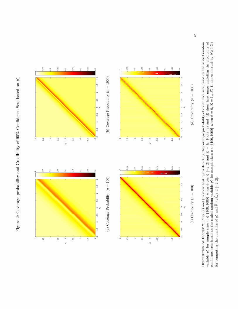
it seems natural to use the same posterior distribution to evaluate the credibilityof the proposed confidence set. Figure 2 reports both the frequentist coverage andthe Bayesian credibility of (1.1), assuming that the Hong and Li (2015) procedureis implemented using the posterior:

θP∗n |Xn ∼ N2( n

n+ 1 θ̂n ,1

n+ 1I2).

The following figure shows that at least in this example fixing coverage comes atthe expense of distorting Bayesian credibility.1

1The Bayesian credibility of CSHn (1− α) is given by:

P∗(g(θP∗n ) ∈ CSHn (1− α)|Xn)

= P∗(g(θ̂n)− 1√

nc∗

1−α/2(Xn) ≤ g(θP∗n ) ≤ g(θ̂n)− 1√

nc∗α/2(Xn)

∣∣∣Xn

)

5

Figu

re2:

Coverag

eprob

ability

andCredibilityof

95%

Con

fiden

ceSe

tsba

sedon

y∗ n

-2-1

.5-1

-0.5

00.

51

1.5

231

-2

-1.5-1

-0.50

0.51

1.52

32

0.6

0.65

0.7

0.75

0.8

0.85

0.9

0.95

1

(a)CoverageProba

bility(n

=10

0)

-2-1

.5-1

-0.5

00.

51

1.5

231

-2

-1.5-1

-0.50

0.51

1.52

32

0.6

0.65

0.7

0.75

0.8

0.85

0.9

0.95

1

(b)CoverageProba

bility(n

=10

00)

-2-1

.5-1

-0.5

00.

51

1.5

2

3̂1

-2

-1.5-1

-0.50

0.51

1.52

3̂2

0.6

0.65

0.7

0.75

0.8

0.85

0.9

0.95

1

(c)Credibility(n

=10

0)

-2-1

.5-1

-0.5

00.

51

1.5

2

3̂1

-2

-1.5-1

-0.50

0.51

1.52

3̂2

0.6

0.65

0.7

0.75

0.8

0.85

0.9

0.95

1

(d)Credibility(n

=10

00)

Des

crip

tion

ofF

igur

e2:

Plots

(a)an

d(b)show

heat

map

sde

pictingthecoverage

prob

ability

ofconfi

dencesets

basedon

thescaled

rand

omvaria

bley

∗ nforsamplesizesn∈{1

00,1

000}

whe

nθ 1,θ

2∈

[−2,

2]an

dΣ

=I 2.Plots

(c)an

d(d)show

heat

map

sde

pictingthecred

ibility

ofconfi

dencesets

basedon

thescaled

rand

omvaria

bley

∗ nforsamplesizesn∈{1

00,1

000}

whe

nθ

=0,

Σ=

I 2,Z

∗ nis

approxim

ated

byN

2(0,Σ

)forcompu

tingthequ

antiles

ofy

∗ nan

dθ̂ n,1,θ̂n,2∈

[−2,

2].

6 KMP

REFERENCES

Dümbgen, L. (1993): “On nondifferentiable functions and the bootstrap,” Probability Theory and

Related Fields, 95, 125–140.

Gelman, A., J. B. Carlin, H. S. Stern, and D. B. Rubin (2009): Bayesian data analysis, vol. 2

of Texts in Statistical Science, Taylor & Francis.

Hong, H. and J. Li (2015): “The numerical delta-method,” Working Paper, Stanford University.

Nadarajah, S. and S. Kotz (2008): “Exact distribution of the max/min of two Gaussian random

variables,” Very Large Scale Integration (VLSI) Systems, IEEE Transactions on, 16, 210–212.