POTENTIAL IMPACTS OF MAN-MADE NOISE ON RINGED SEALS: VOCALIZATIONS AND REACTIONS by William C. Cummings Oceanographic Consultants D. V. Holliday B. J. Lee Tracer, Inc. Final Report Outer Continental Shelf Environmental Assessment Program Research Unit 636 December 1984 95
Transcript
POTENTIAL IMPACTS
OF MAN-MADE NOISE ON RINGED SEALS:
VOCALIZATIONS AND REACTIONS
by
William C. CummingsOceanographic Consultants
D. V. HollidayB. J. Lee
Tracer, Inc.
Final ReportOuter Continental Shelf Environmental Assessment Program
Research Unit 636
December 1984
95
jngciuã1(1102
I2fI2Tct
TABLE OF CONTENTS
Section Page
L I S T O F T A B L E S . . . . . . . . . . . . . . 0 . . . 0 9 9
LIST OF FIGURE S...... . . . . . . . . . ...101
I. EXE CUT IVE SUMMARY .“. ... ., . . . ..O O. ..107
Table 1. Playback schedule of previously recorded underwaterman-made noise, Kotzebue Sound, 1984.
Table 2. Listing of ringed seal sound categories and theiroccurrence as to location and proportion.
Table 3. Occurrence of infrequent ringed seal vocalizationcategories from the triangular array period, 25 March- 11 April 1984.
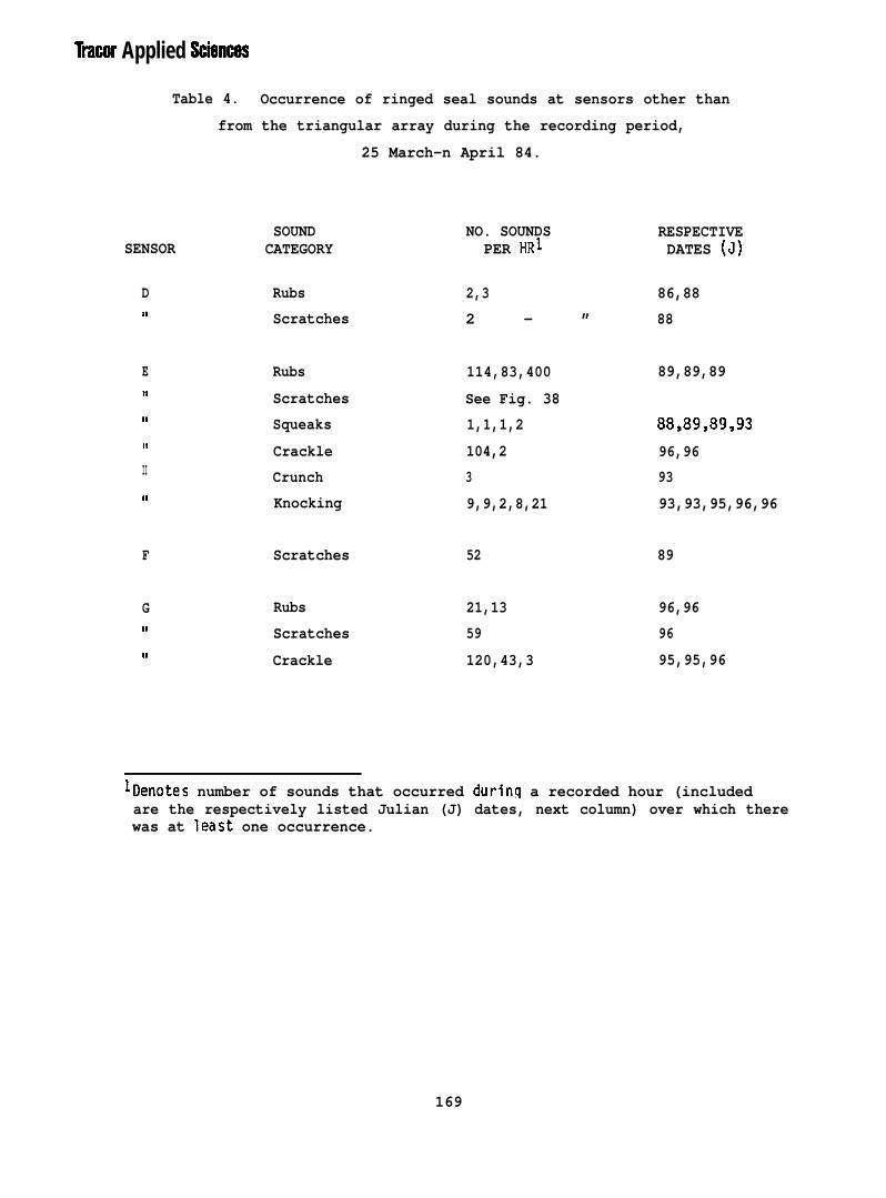
Table 4. Occurrence of ringed seal sounds at sensors other thanfrom the triangular array during the recording period,25 March - 11 April 1984.
Table 5. Compilation of bearings and range of some soundsselected for localization, referenced to hydrophore A.
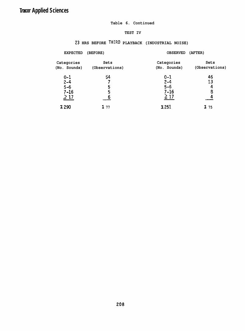
Table 6. Data base for chi square tests of independence.
Table 7. Summary of chi square single classification tests ofindependence for the occurrence of ringed sealvocalizations before and after designated playbackexperiments.
99—
LIST OF FIGURES
Figure 1.
Figure 2.
Figure 3.
Figure 4.
Figure 5.
Figure 6.
Figure 7.
Figure 8.
Figure 9.
Figure 10.
Figure 11.
Figure 12.
Figure 13.
Study site (arrow) at’the offshore edge of KotzebueSound, Alaska.
Schematic, modifications, and specifications of thetelemetry units.
Sketch of recording site layout with distances anddirections from camp (drawing not to scale).
Histogram showing pooled monitoring (recording)effort.
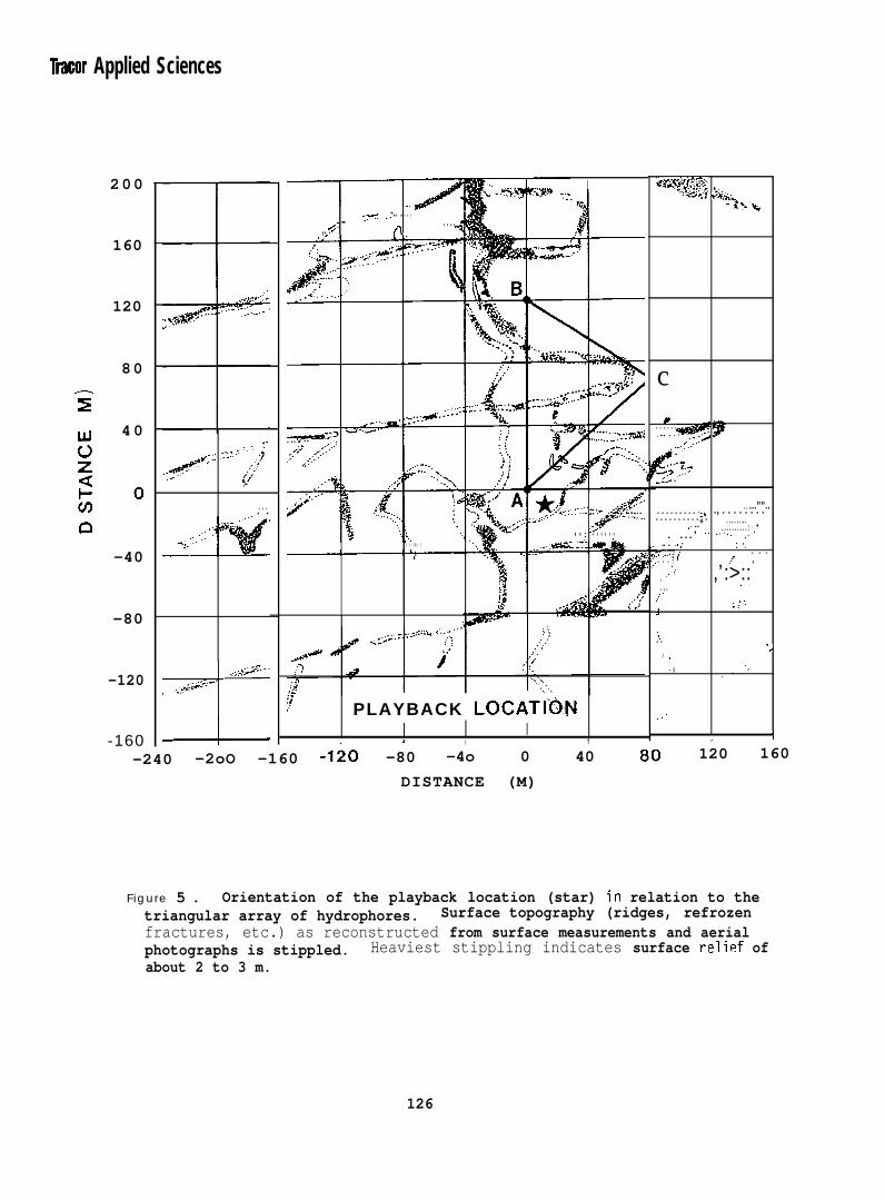
Orientation of the playback location (star) inrelation to the triangular array of hydrophores.Surface topography (ridges, refrozen fractures, etc.)as reconstructed from surface measurements and aerialphotographs is stippled. Heaviest stipplingindicates surface relief of about 2 to 3 m.
Waterfall display (time history) of Vibroseis andassociated industrial noise playback, recorded on thetriangular array, showing the fundamental and up tothe llth harmonic, analyzing filter bandwidth. 7.5Hz.
Instantaneous spectra (upper) and 15 sec duration ofpeak hold spectra (lower) of seismic explorationconvoy noise playback consisting of D-6 cat scrapingice, drill, and trucks. Analyzing filter bandwidth18.8 Hz and 37.5 Hz, respectively.
Voltage plotted as a function of time for a transientsound due to ice cracking (upper). Another transient(lower) is displayed with a time scale that is 200times faster than the waveform in the upper figure.
Relative power spectrum density of an ice-crackingsound.
Sensor locations (A,B,C), ice ridges (stippled),triangular array, and the intersection of twoparabolas (star) based on the indicated sound arrivaltime differences.
Arrivals of the same ice cracking transient sound athydrophores A and C (upper) and their crosscorrelation function used to determine the arrivaltime difference, 72.27 ms (lower).
Waveform (upper) and spectrum (lower) of a singlescratch sound, 30 March 1984. Analyzing filterbandwidth was 3.75 Hz (upper) and 37.5 Hz (lower).
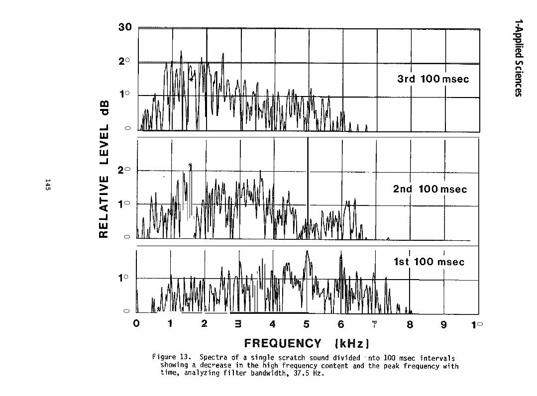
Spectra of a single scratch sound divided into 100msec intervals showing a decrease in the highfrequency content and the peak frequency with time,analyzing filter bandwidth, 37.5 Hz.
Figure 14.
Figure 15.
Figure 16.
Figure 17.
Figure 18.
Figure 19.
Figure 20.
Figure 21,
Figure 22.
Figure 23.
Figure 24.
Figure 25.
Figure 26.
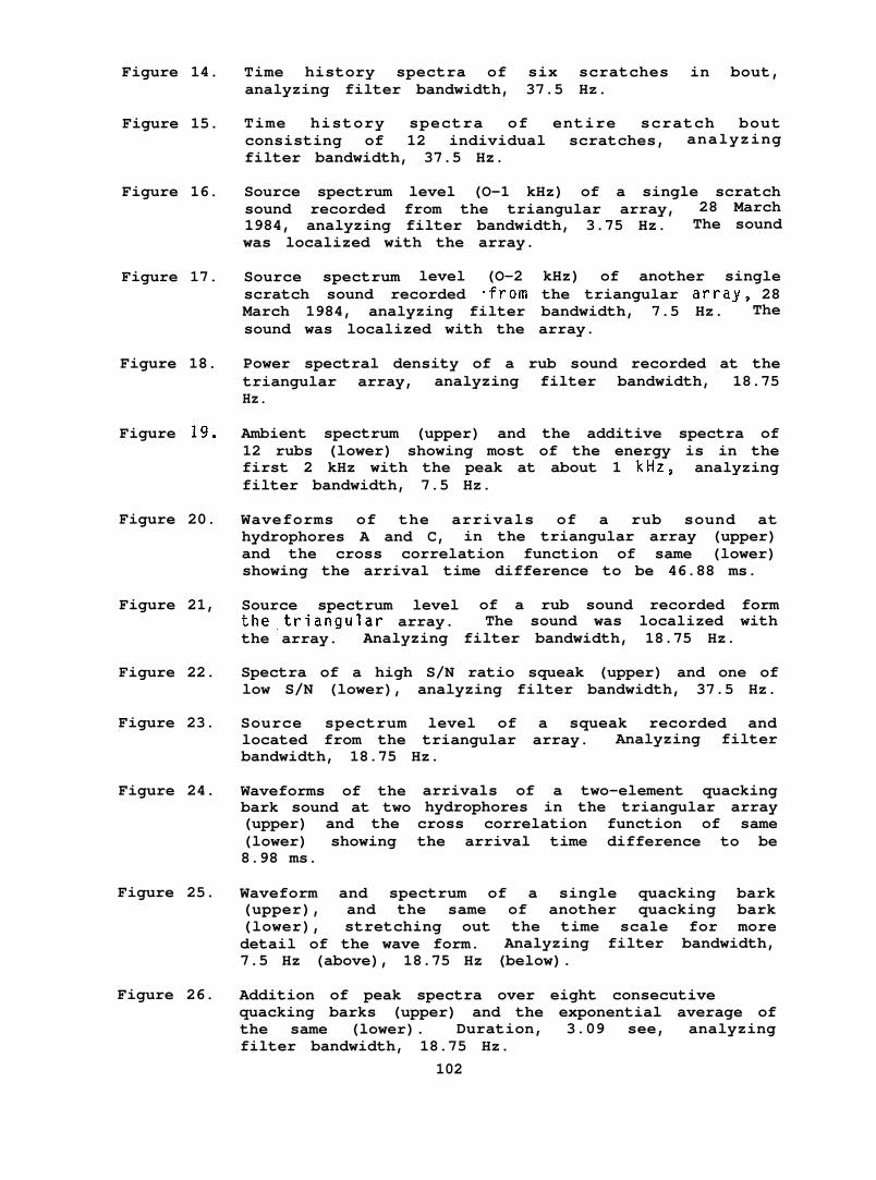
Time history spectra of six scratches in bout,analyzing filter bandwidth, 37.5 Hz.
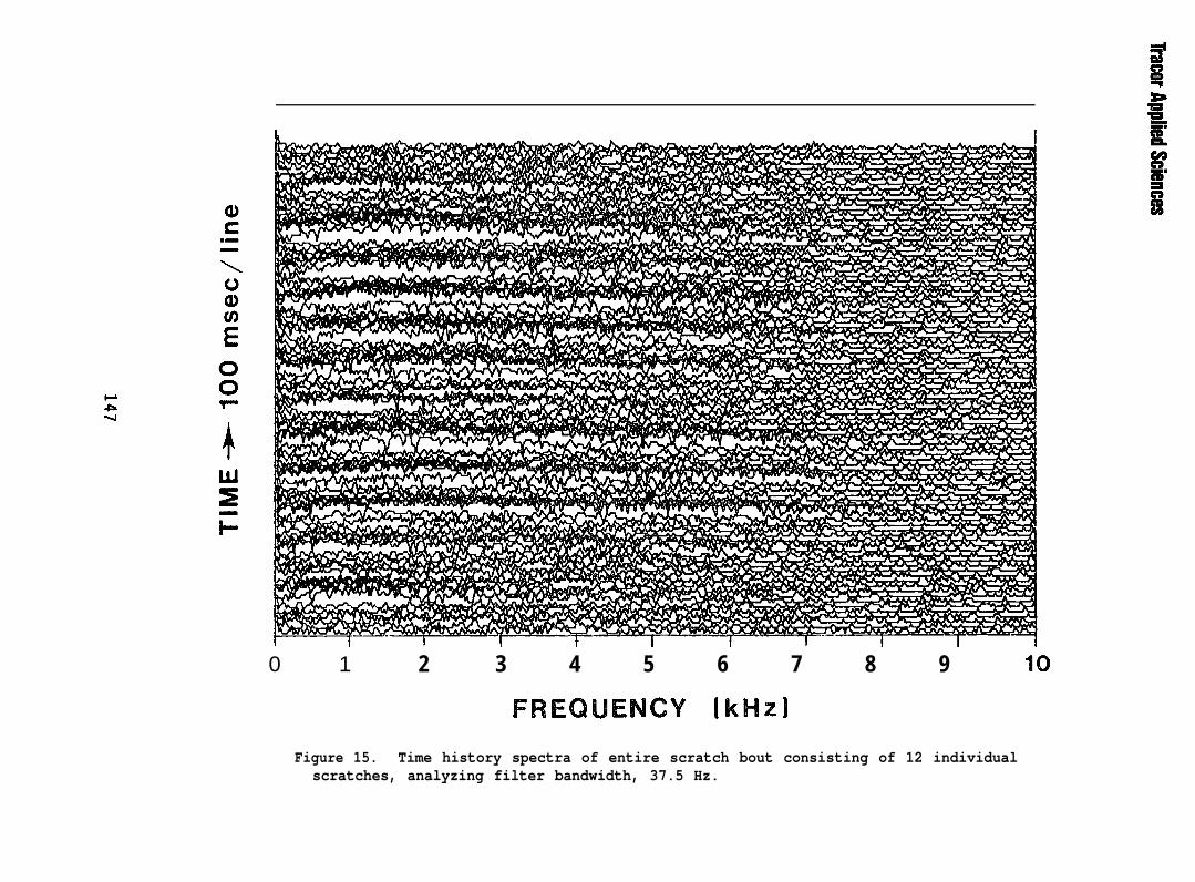
Time history spectra of entire scratch boutconsisting of 12 individual scratches, analyzingfilter bandwidth, 37.5 Hz.
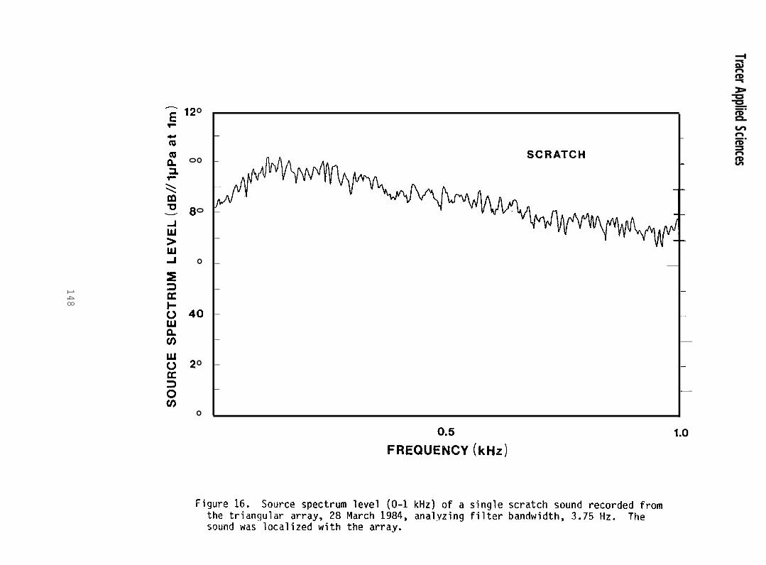
Source spectrum level (O-1 kHz) of a single scratchsound recorded from the triangular array, 28 March1984, analyzing filter bandwidth, 3.75 Hz. The soundwas localized with the array.
Source spectrum level (O-2 kHz) of another singlescratch sound recorded “from the triangular array~ 28March 1984, analyzing filter bandwidth, 7.5 Hz. Thesound was localized with the array.
Power spectral density of a rub sound recorded at thetriangular array, analyzing filter bandwidth, 18.75Hz.
Ambient spectrum (upper) and the additive spectra of12 rubs (lower) showing most of the energy is in thefirst 2 kHz with the peak at about 1 kHz, analyzingfilter bandwidth, 7.5 Hz.
Waveforms of the arrivals of a rub sound athydrophores A and C, in the triangular array (upper)and the cross correlation function of same (lower)showing the arrival time difference to be 46.88 ms.
Source spectrum level of a rub sound recorded formthe,triangular array. The sound was localized withthe array. Analyzing filter bandwidth, 18.75 Hz.
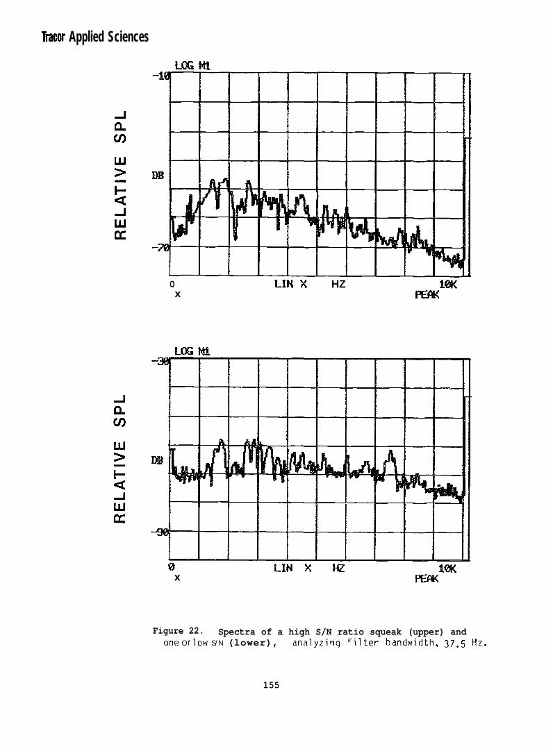
Spectra of a high S/N ratio squeak (upper) and one oflow S/N (lower), analyzing filter bandwidth, 37.5 Hz.
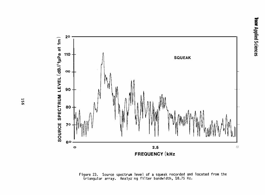
Source spectrum level of a squeak recorded andlocated from the triangular array. Analyzing filterbandwidth, 18.75 Hz.
Waveforms of thebark sound at two(upper) and the(lower) showing8.98 ms.
arrivals of a two-element quackinghydrophores in the triangular arraycross correlation function of samethe arrival time difference to be
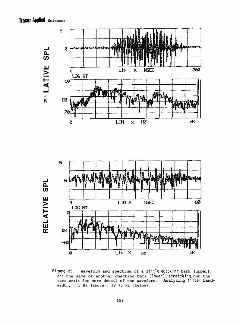
Waveform and spectrum of a single quacking bark(upper), and the same of another quacking bark(lower), stretching out the time scale for moredetail of the wave form. Analyzing filter bandwidth,7.5 Hz (above), 18.75 Hz (below).
Addition of peak spectra over eight consecutivequacking barks (upper) and the exponential average ofthe same (lower). Duration, 3.09 see, analyzingfilter bandwidth, 18.75 Hz.
102
Figure 27.
Figure 28.
Figure 29.
Figure 30.
Figure 31.
Figure 32.
Figure 33.
Figure 34.
Figure 35.
Figure 36.
Spectrum of a single quacking bark analyzed at peakamplitude (upper), analyzing filter bandwidth, 18.75Hz. Power spectral densities (O-1 kHz) of thearrival of a quacking bark at two hydrophores in thetriangular array, analyzing filter bandwidth, 3.7 Hz.
Source spectrum level of a quacking bark recorded andlocated with the triangular array. Analyzing filterbandwidth, 7.5 Hz.
Histogram showing the long-term increase in the rateof ringed seal vocalizations from the array (sounds,excluding scratches) over the recording periodbeginning with Julian day 86 (26 March 1984). Thedata were normalized for unequal recording times eachday (see text).
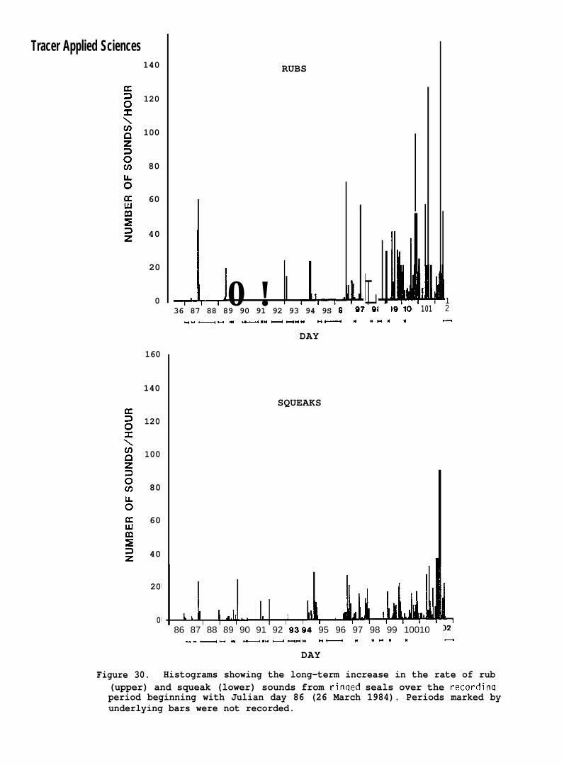
Histograms showing the long-term increase in the rateof rub (upper) and squeak (lower) sounds from ringedseals over the recording period beginning with Julianday 86 (26 March 1984). Periods marked by underlyingbars were not recorded.
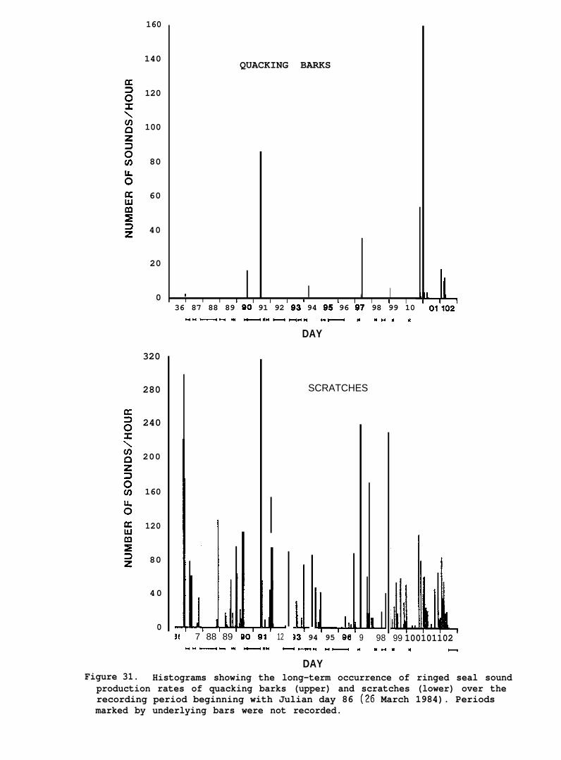
Histograms showing the long-term occurrence of ringedseal sound production rates of quacking barks (upper)and scratches (lower) over the recording periodbeginning with Julian day 86 (26 March 1984).Per-iods marked by underlying bars were not recorded.
Histogram of pooled data involving all soundcategories at the triangle, including scratches,recorded over the entire period beginning with Julianday 86 (26 March 1984).
Histograms showing the hourly occurrence of allringed seal sounds from the triangular array, pooledover the number of days indicated and normalized forunequal numbers of recordings (upper) and the samedata smoothed by a moving average of 3 (lower).
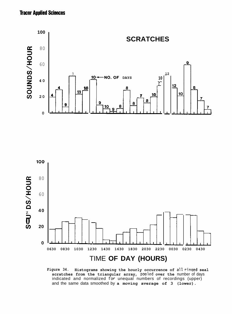
Histograms showing the hourly occurrence of allringed seal scratches from the triangular array,pooled over the number of days indicated and normal-ized for unequal numbers of recordings (upper) andthe same data smoothed by a moving average of 3(lower).
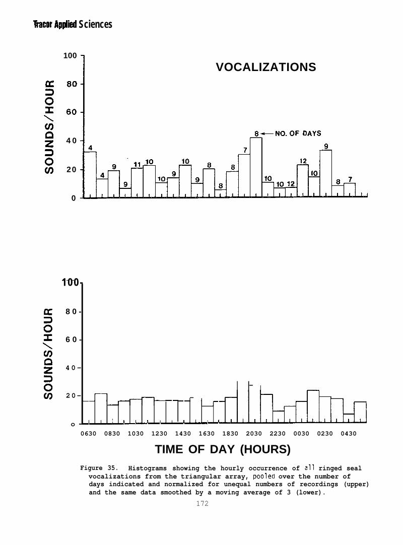
Histograms showing the hourly occurrence of allringed seal vocalizations from the triangular array,pooled over the number of days indicated and normal-ized for unequal numbers of recordings (upper) andthe same data smoothed by a moving average of 3(lower).
Fast Fourier Transform (FFT) of the frequency ofoccurrence of ringed seal vocalizations (sounds,excluding scratches) showing two possibleperiodicities of about 7 and 2 hours (from pooleddata of 3,359 vocalizations at the triangle).
103
Figure 37.
Figure 38.
Figure 39.
Figure 40.
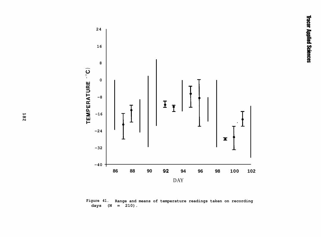
Figure 41.
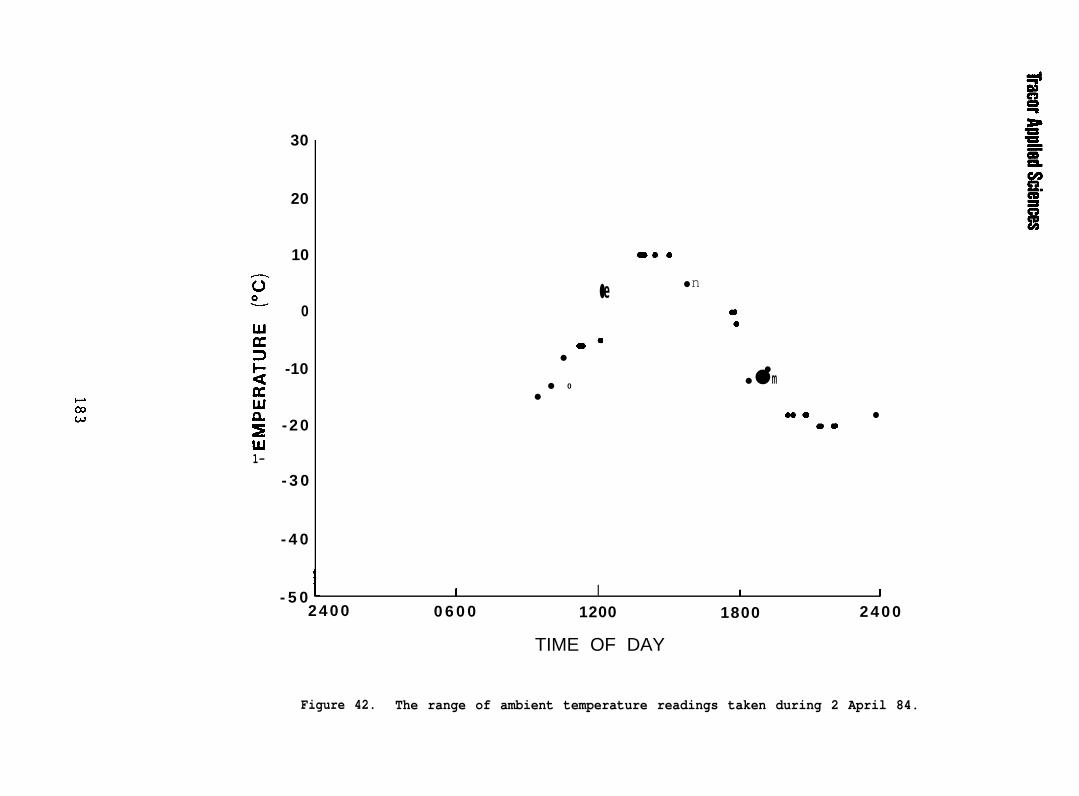
Figure 42.
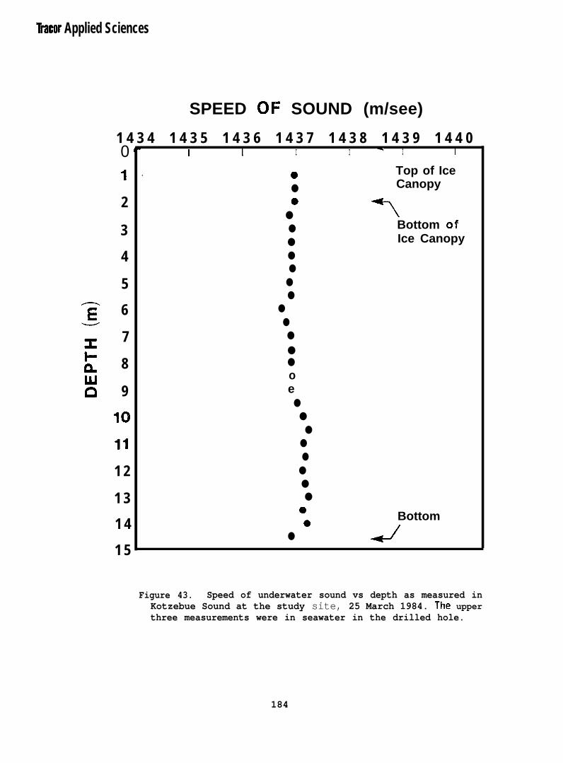
Figure 43.
Figure 44.
Figure 45.
Figure 46.
Figure 47.
Figure 48.
Figure 49.
Figure 50.a
Figure 51.
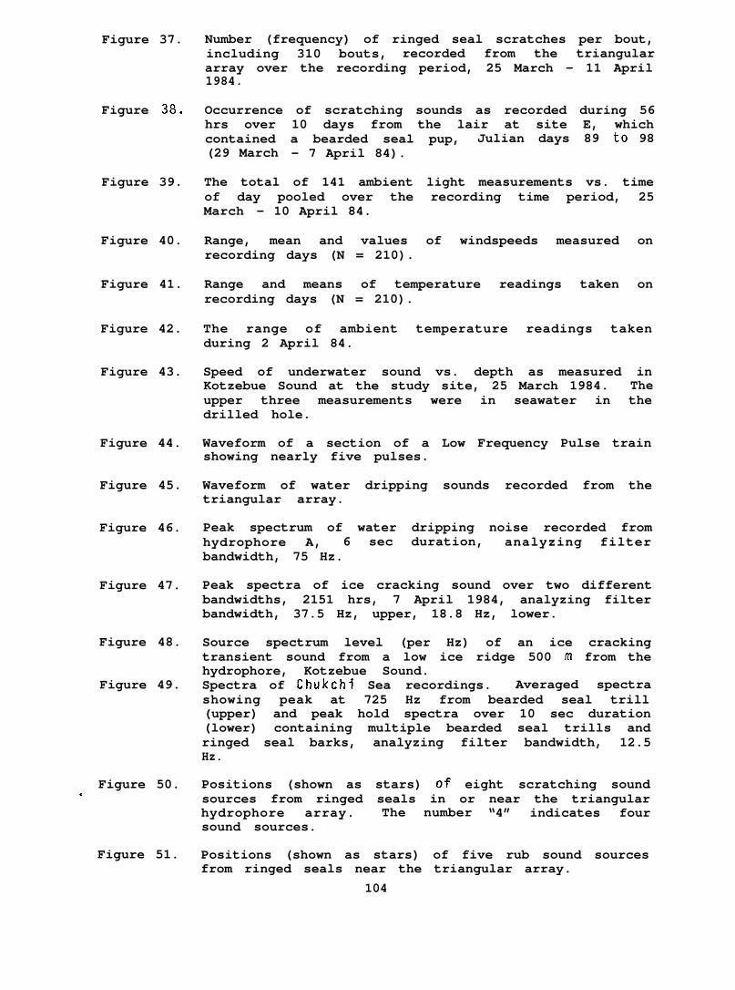
Number (frequency) of ringed seal scratches per bout,including 310 bouts, recorded from the triangulararray over the recording period, 25 March - 11 April1984.
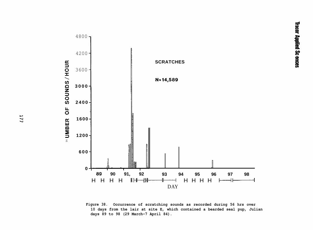
Occurrence of scratching sounds as recorded during 56hrs over 10 days from the lair at site E, whichcontained a bearded seal pup, Julian days 89 to 98(29 March - 7 April 84).
The total of 141 ambient light measurements vs. timeof day pooled over the recording time period, 25March - 10 April 84.
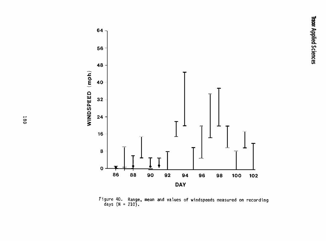
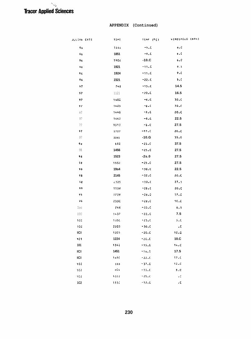
Range, mean and values of windspeeds measured onrecording days (N = 210).
Range and means of temperature readings taken onrecording days (N = 210).
The range of ambient temperature readings takenduring 2 April 84.
Speed of underwater sound vs. depth as measured inKotzebue Sound at the study site, 25 March 1984. Theupper three measurements were in seawater in thedrilled hole.
Waveform of a section of a Low Frequency Pulse trainshowing nearly five pulses.
Waveform of water dripping sounds recorded from thetriangular array.
Peak spectrum of water dripping noise recorded fromhydrophore A, 6 sec duration, analyzing filterbandwidth, 75 Hz.
Peak spectra of ice cracking sound over two differentbandwidths, 2151 hrs, 7 April 1984, analyzing filterbandwidth, 37.5 Hz, upper, 18.8 Hz, lower.
Source spectrum level (per Hz) of an ice crackingtransient sound from a low ice ridge 500 m from thehydrophore, Kotzebue Sound.Spectra of Chukchi Sea recordings. Averaged spectrashowing peak at 725 Hz from bearded seal trill(upper) and peak hold spectra over 10 sec duration(lower) containing multiple bearded seal trills andringed seal barks, analyzing filter bandwidth, 12.5Hz.
Positions (shown as stars) of eight scratching soundsources from ringed seals in or near the triangularhydrophore array. The number “4” indicates foursound sources.
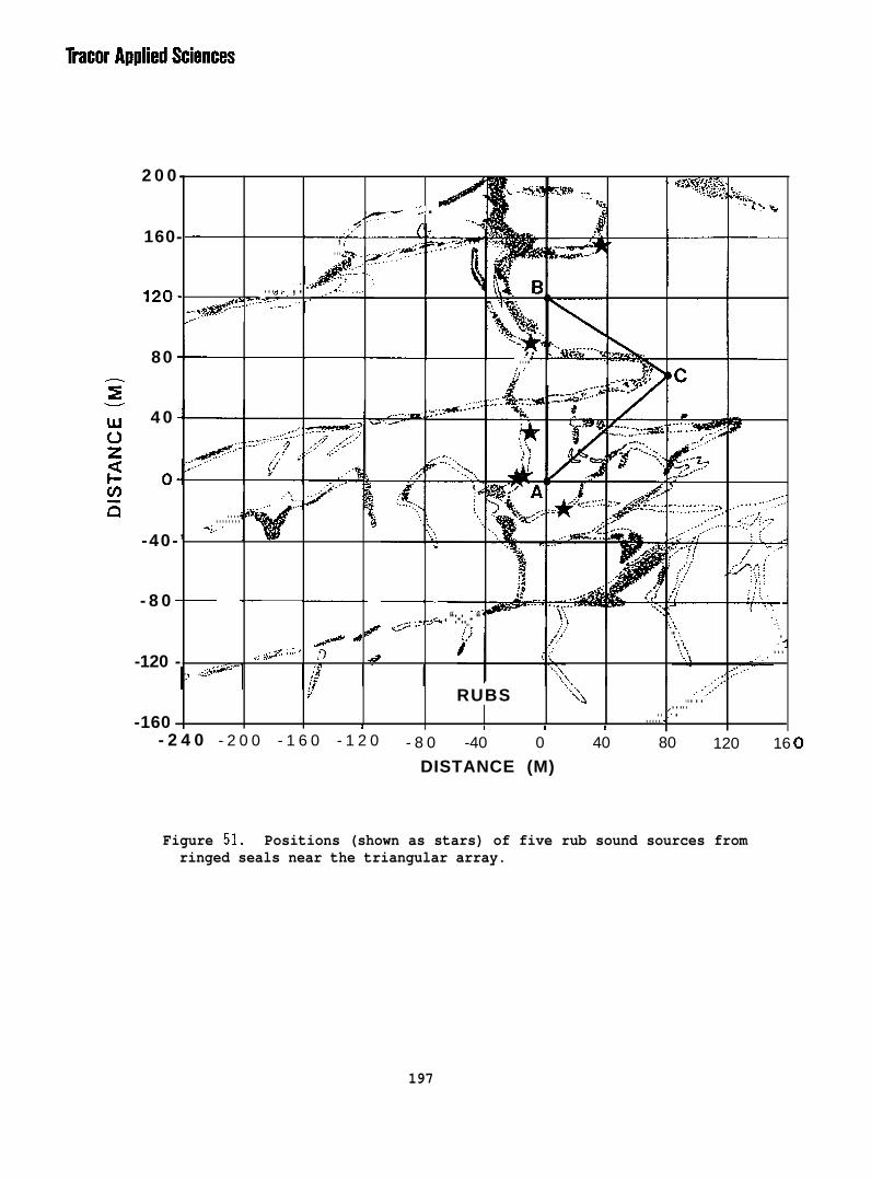
Positions (shown as stars) of five rub sound sourcesfrom ringed seals near the triangular array.
104
Figure 52. Positions (shown as stars) of two squeak s o u n dsources from ringed seals in or near the triangulararray.
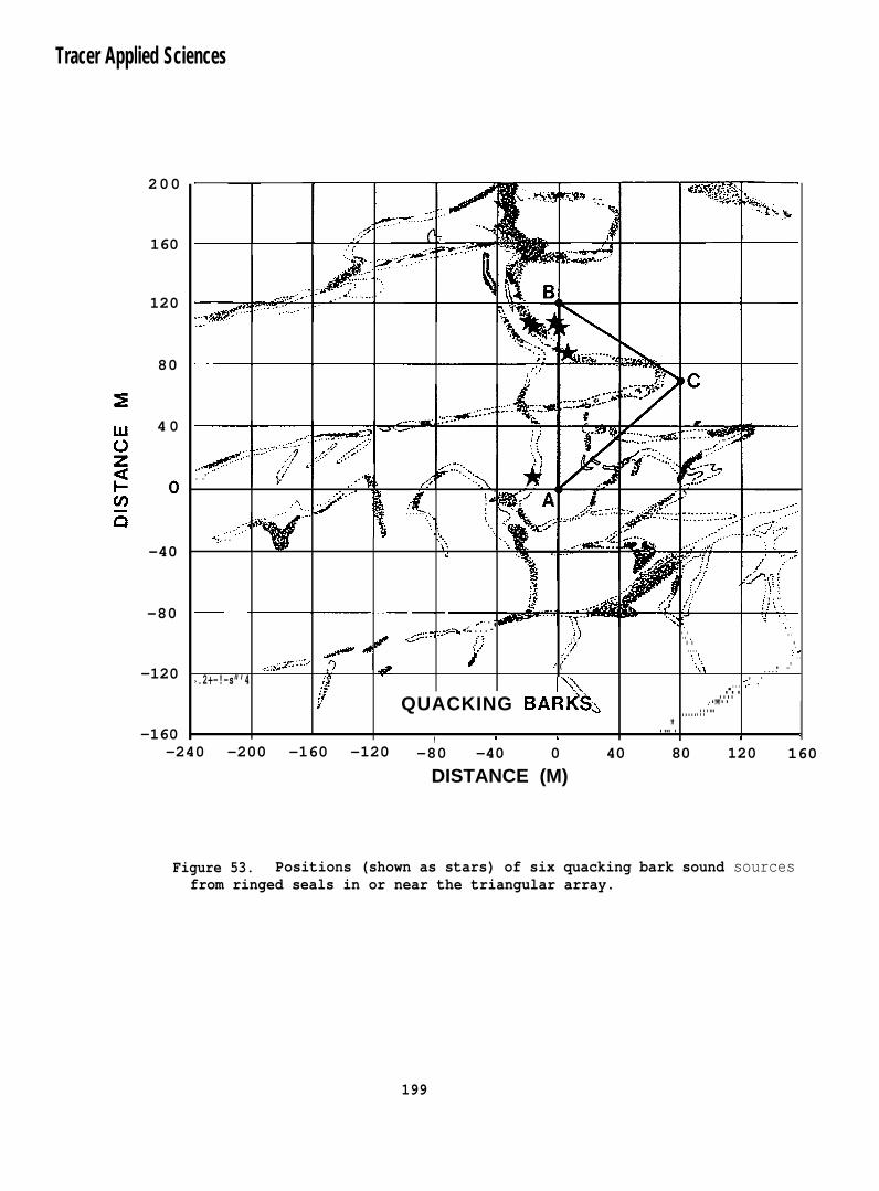
Figure 53. Positions (shown as stars) of six quacking bark soundsources from ringed seals in or near the triangulararray.
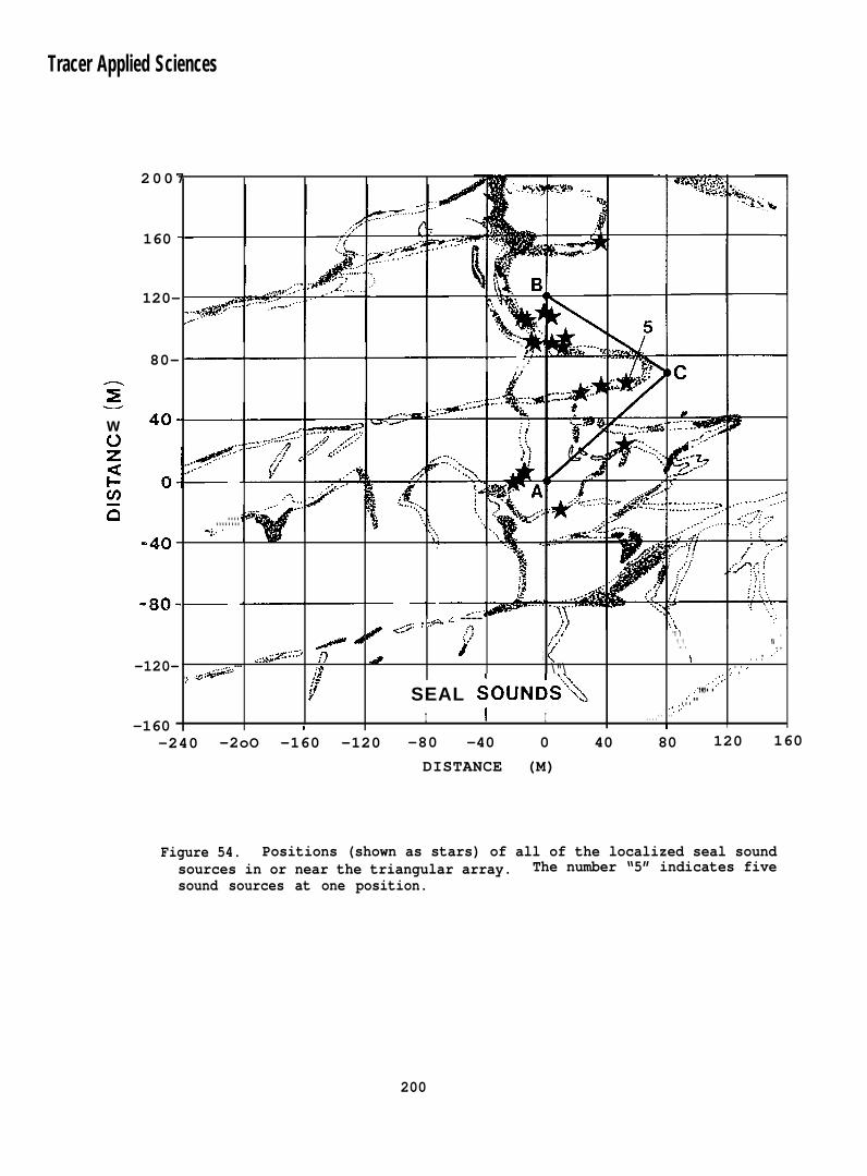
Figure 54. Positions (shown as stars) of all of the localizedseal sound sources in or near the triangular array.The number “5” indicates five sound sources.
Figure 55. Positions of nine ice cracking sound sources (stars)near the triangular array.
Figure 56. D i s t r i b u t i o n o f n u m b e r s o f r i n g e d sealvocalizations/15 min periods over 72 hrs before anyplayback of man-made noise (upper) and 72 hrs afterall playbacks (lower).
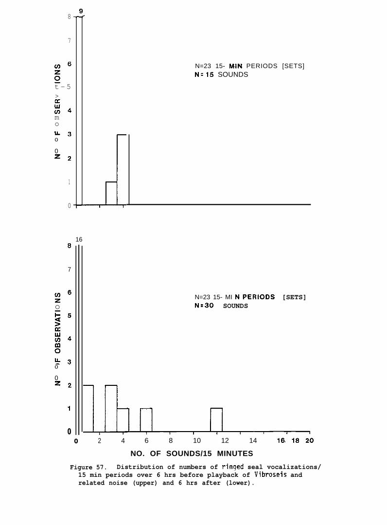
Figure 57. D i s t r i b u t i o n o f n u m b e r s o f r i n g e d sealvocalizations/15 min periods over 6 hrs beforeplayback of Vibroseis and related noise (upper) and 6hrs after (lower).
Figure 58. D i s t r i b u t i o n o f n u m b e r s o f r i n g e d sealvocalizations/15 min periods over 10 hrs beforeplayback of random and 1 kHz noise (upper) and 10 hrsafter (lower).
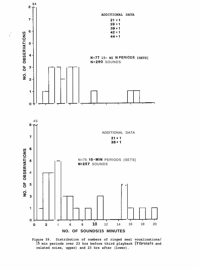
Figure 59. D i s t r i b u t i o n o f n u m b e r s o f r i n g e d sealvocalizations/15 min periods over 23 hrs before thirdplayback (Vibroseis and related noise, upper) and 23hrs after (lower).
105
?mcor Applied Schmes
I. EXECUTIVE SUMMARY
This is a report of studies related to possible impacts of man-made
noise on the ringed seal (Phoca hispida), with emphasis on seal vocaliza-
tions and noises associated with near-shore geophysical exploration. The
research was supported by the Minerals Management Service through inter-
agency agreement with the National Oceanic and Atmospheric Administration,
Office of Oceanography and Marine Services, Juneau, Alaska, as part of the
Outer Continental Shelf Environmental Assessment Program under Contract83-ABC-00065. It was conducted in Kotzebue Sound, Alaska, during March
and April 1984.
The study area was typical of that used or planned for offshore
seismic exploration. It was covered with first-year landfast ice,
deformed with ridges, hummocks, and refrozen fractures, in a shallow-
water area found to be inhabited with ringed seals. Surprisingly, there
was evidence that at least two bearded seals (Erignathus barbatus) also
resided there. A bearded seal pup was found in a lair, and very distant
bearded seal trills were recorded on two occasions. The major task was
to characterize the types of ringed seal sounds in this location by means
of long-term field recordings, and to determine their frequency of occur-
rence as a possible clue to any changes in sound production resulting
from the artificial introduction of “industrial” underwater noise.
The field activities centered on a precisely located
array, which resulted in not only a very large number of
but some Vocalizations of sounds and sound source levels
3-hydrophore
recorded hours,
(intensity).
Data were also obtained from outlying hydrophores, including a recording
192 km away. Not counting duplications on recordings of up to six hydro-
phores at once, we recorded and monitored 245 hrs of data, comprising
nearly 25,000 biological sounds.
Ringed seal sounds were of comparatively low source level. Located
seal and ice sounds originated mostly in areas of active ice, i.e.,
refrozen fractures or ridges, at distances up to 0.6 km. The frequency
107
Tmcor Applied Sciences
of occurrence of vocalizations dramatically increased over the study,
presumably as breeding and parental activity increased. Ice scratching
occurred mostly at two times of the day, and the occurrence of vocaliza-
tions also showed dependence on time of day. More vocalizations occurred
during daylight hours. There were more vocalizations during periods of
low windspeed, perhaps the effect of decreased aural masking by wind
generated noise for the human listener. The number of scratches was not
correlated with windspeed or temperature. The number of vocalizations
increased during lower temperatures. Temperature and windspeed were not
statistically correlated.
The rubs, squeaks, and quacking barks recorded by us appear to be very
similar to ringed seal” sounds described by Stirling and coworkers.
The results of underwater noise playback had to be considered in
light of an overlying long-term natural inGrease in sound production.
Consequently, comparable periods were kept reasonably short. Two compari-
sons before and after playback (6 and 23 hrs) of recorded “industrial”
noise showed no statistical difference in sound production. Two other
periods of comparison before and after (10 and 72 hrs) showed that sound
production increased after playbacks, possibly related to an expected
overall heightening of breeding and parental activity as the season
progressed. There is a possibility that noise unassociated with our
activity intensified ringed seal sound production based on the initial-
ization of certain vocalizations by distant sources of low frequency
pulses supposedly of man-made origin.
Recommendations basically involve the need for more research with
narrower focusing, i.e., sound propagation, attenuation and modeling
studies, and more controlled experimentation. Based upon this study,
there was no evidence that petro-exploratory industrial noise reduced the
occurrence of sound production of ringed seals. In some instances, it
could have increased sound production. For example, a different kind of
noise (low frequency pulsing believed to be of man-made origin) incited
ringed seals to produce rub, squeak and quacking bark sounds. Since the
source levels of ringed seal sounds were relatively low, there could have
been a potential indirect effect from acoustical masking.
108
Compared to other pinnipeds,
izations under the circumstances
ringed seals did not produce many vocal-
of this study. Consequently, future
research that is intended to utilize vocal sound production as indices to
population enumeration, distribution or behavior may, of necessity, be
limited. On the other hand, ice scratching sounds were very common, and
they could possibly be used for these purposes.
109
Tktcor Applied !Mcmes
11. INTRODUCTION AND BACKGROUND
The ProblemA.
reg.
Ringed seals, Phoca hispida, are extremely abundant in Arctic Polar
ens. Of all the marine mammals of this region, this species s the
most numerous and widespread, being circumpolar in distribution (King,
1964). In recent years there has been a large-scale development of
hydrocarbon energy sources in the near- and on-shore regions of Arctic
Alaska. Associated with industrial activities involving exploration,
development, and production, are increased levels of man-made noise and
vibration (Malme and Miawski, 1979; Holliday et al., 1980, 1983, 1984;
Cummings et al., 1981(6 references); Cummings & Holliday, 1983(3 references);
Green, 1981; Ljundblad, 1983; Turl, 1982; LGL, 1981). Please refer to J.
Acoust. Sot. Am., Suppl 1, Vols. 70, 74 for abstracts of other reports on
man-made underwater noise based on work outside of the Alaskan Arctic
region.
Airborne
of potential
noise and vibration from petro-industrial activities may be
impact on Arctic wildlife; in particular, the ringed seal.
OCSEAP has expressed concern that noisy activities could adversely affect
the bioacoustical behavior of ringed seals, especially during the
sensitive period of their life cycle as pups or mothers in early spring
reproductive activities. A major source of noise in certain of Alaska’s
coastal ice regions is associated with on-ice geophysical exploration
wherein low frequency sound is used to detect deposits of hydrocarbons in
the underlying strata. Added to the noise from seismic profiling itself,
are numerous other noise sources such as bulldozers, tank trucks, ice
drilling rigs, and transport vehicles.
In addition to possible lair abandonment or displacement (ASA, 1980),
the effects of man-made noise may be manifested as changes in the vocal
behavior that presumably is important to the animals’ welfare. For
example, sound production in birds and fish has been shown to cease in
the presence of loud man-made noise. There is also an indication thatthe frequency of occurrence of gray whale sounds is affected by man-made
110
noise (Malme et al., 1983, 1984). The sound production of ringed seals
could possibly be affected, but before any changes could be detected in
their vocal behavior, a ground truth data base must be established.
Thus, the main purpose of this research was to study the ringed seal’s
vocal activities, first, in a relatively undisturbed situation, and
second, when the animals were exposed to possibly disturbing man-made
noise. Hopefully, the work would yield information on apparent
behavioral roles of vocalizations.
The Alaska office of OCSEAP and the Alaska Eskimo Whaling Commission
(AEMC) contracted with Oceanographic Consultants and Tracer in 1981 for
the purpose of developing an underwater sound localization system for
ringed seal studies and for measurement of Vibroseis@ 1 seismic
profiling noise. The results of that work are described in a report by
Cummings, et al. (1981). In 1983, OCSEAP supported our studies on
acoustic and vibration measurements related to possible disturbance of
ringed seals off Prudhoe Bay (Holliday et al., 1984). The present study
was funded via a prime contract with Tracer, Inc., and a subcontract to
Oceanographic Consultants.
B. The Ringed Seal and Its Bioacoustics
Although ringed seals are circumpolar in distribution, significantly
large numbers occur on or very near landfast ice during the winter months
(King, 1964). They are an important species to Inuit cultures because of
their abundance and use for food, shelter, clothing, and artifacts
(D. Brice-Bennett, Inuit Tapi risat of Canada, pers. communication).
Male and female ringed seals grow to about the same size (90 kg,
1.4 m) and may live to be over 40 years of age. The pups are born during
a period from about mid-March to mid-April. Birth takes place in anatural ice cave or in a lair excavated by the mother where an access
lThe use of trade names or model numbers in this report does not implyendorsement.
111
hole is kept open. Other holes are kept open only for the purpose of
breathing. Ringed seal pups are greatly dependent upon their mothers for
nourishment, and they nurse for about eight weeks (Scheffer, 1958;
McLaren, 1958; Burns and Eley, 1976).
Ringed seals feed on crustaceans and small fish. Their enemies
include killer whales, polar bears, Arctic foxes, man, and pathogens
(King, 1964).
Smith and Stirling (1975) described the wide variety of lairs as being
composed of two general types. They also described the process by which
they are constructed. One type, the birth lair, probably originates with
the other, the haul-out lair. Birth lairs may have tunnels, whereas
haul-out lairs generally are a single chamber. Lairs provide thermal
insulation and a hiding place from polar bears and foxes. The reported
lair sizes varied from 45 - 65 cm high, 196 - 355 cm long, and 135 -
227 cm wide. These authors indicated that populations may be limited by
the amount of suitable breeding ice.
The hearing capabilities of seals were given an early review by Mohl
(1968). Terhune and Ronald (1975a, 1975b, 1976) reported on the hearing
of ringed seals and the following is mostly based upon their work. There
is virtually no quantitative information on the sensitivity of seals to
vibrational energy (displacement of the medium vs hearing).
We can assume that the audiogram of ringed seals is U-shaped; however,
due to technical difficulties in producing uniform low-frequency sound
fields at known received levels in small underwater enclosures, hearing
sensitivity below about 1 kHz has not been measured. However, ringed
seals do produce (and presumably hear) sound below 1 kHz (Cummings et
al., 1981). Terhune and Ronald reported a fairly uniform sensitivity (~
7 dB) from 1 to 45 kHz, with increases of about 60 d13/octave above that
frequency to 90 kHz. Thresholds below 45 kHz are about -30 to -20 dB re
lpbar (70 to 80 dB re luPa). Critical ratios vary between 30~5.4 dB
(at 4 kHz) to 35 ~ 4.5 dB (at 32 kHz). Critical bandwidths over thesefrequencies vary from 1 to 3.16 kHz. They concluded that the loss of
112
both sensitivity and pitch discrimination effectively places the upper
limit of useful hearing at 90 kHz. On this basis, ringed seals are
capable of hearing noise spectra above 1 kHz that is associated with gas
and oil exploration on the ice. It would be difficult to predict the
masking effect of this noise on their own sounds without more research.
Most animals produce a lexicon of sounds which may occur in well-
defined patterns. Examples are the long, involved repetitions of hump-
back (Payne) and bowhead whale (Ljungblad et al., 1982; Cummings et al.,
1983) sounds, or the rhythmical sounds of wild porpoises. We (Hell iday
et al., 1980) have shown that bearded seal calls off Barrow, Alaska,
occurred in a diurnal pattern. The ability to recognize patterns implies
categorization and recognition of the components, which can be described
in physical terms such as frequency, temporal, and amplitude character-
istics.
Very little information has been published on ringed seal sounds.
Stirling (1973) described barks, yelps, high-pitched growls, and chirps
of ringed seals that extended up to a maximum of about 6 kHz. Cummings
et al. (1981) presented some spectra of ringed seal sounds: a gargle-
type with peak energy at 1 kHz, a rub that extended from about 0.7 -
2.6 kHz, a bubbling sound thought to have been produced from an underwater
exhalation, .05 - 11 kHz, and a scratching sound from a ringed seal work-
ing on its breathing or access hole, or in the lair above, 0.5 - 3 kHz.
Stirling, et al. (1983), observed that ringed seal vocal izations were
more frequent in late April than earlier in the season or in late June,
and that the sounds have the potential of being useful for information on
distribution and abundance. Their sonagrams indicated considerable low
frequency energy in the ringed seal’s sounds, below 500 Hz.
Although the behavioral significance of these sounds is unknown, we
may assume that some sounds involve inter-animal communications. Likely
functions of the signals doubtlessly are associated with courtship,
parent-offspring, food finding, and territorial behavior. Based upon
113
Thor A@id Sck?ms
what is known of the importance of sound production in other species, it
could be assumed, a priori, that ringed seal sound production is a
requirement for survival in the natural environment.
To our knowledge, man-made noise had not previously been experi-
mentally played back to ringed seals. Watkins and Schevill (1968) used
playbacks to Weddell seals that consisted of the seals’ sounds. They
reported varied responses and described an apparent learning to ignore.
Cummings played back killer whale sounds and random noise to California
sea lions off Catalina Island and in the Gulf of California in an unsuc-
cessful attempt to displace them from fishing operations (unpublished).
There either was no apparent reaction or the seals appeared to be
attracted to the underwater transducer. P. Shaughnessy had much the same
results in experiments
in South Africa (pers.
and co-workers, Oregon
underwater playback of
for the same purpose with fur seals and sea lions
communication). On the other hand, Dr. Bruce Mate
State University, have experienced success with
noise to harbor seals in the attempt to reduce
their predation upon salmon in a restricted area (personal communication).
Schusterman and Moore (1981) stressed the importance of individual and
group behavioral variability of response to noise.
c. Acoustic Environment
Most models involving the reception of acoustic energy will include
three basic parameters, the received level (RI-), total propagation losses
(TL), and the source level (SL). Thus RL will depend upon the degrada-
tion of the propagated sound (TL) and the power of that sound at its
source (SL). The most simplified expression of this relationship is:
R L = S L - T L (eq. 1)
where all three variables are given in decibels (dB). As used in this
report,
dB = 20 lo9@~/PfJ (eq. 2)
114
Tmcor Applied %ienws
where PI signifies measured acoustic pressure and PO signifies a
reference of the pressure measurement, herein defined as 1 pPa (one
micropascal). While the dB may seem to be a very indirect method of
indicating acoustic levels, it is used by convention because the normal
range in pressure units may be in the millions. Since the dB is actually
a multiple of a logarithm, its unit is much more manageable in acoustic
measurements than the unwieldy large numbers encountered
measurement of pressure, the physical stimulus perceived
in the direct
by the ear.
Also by convention, the term “signal” as applied here denotes the
sound of interest, e.g., the warning bark of a seal, whereas the back-
ground or accompanying sound may be termed “noise”. In most applica-
tions, it is the reseacher’s arbitrary choice to define sound(s) as
signal or noise. In practice, this choice usually does not depend
aural pleasure or discrimination.
At first glance of eq. 1, it may appear that the loudness of a
upon
received level (RL) to a listener will depend upon its magnitude, source
level, and total propagation loss. While all three variables are
involved in auditory perception, given a satisfactory receiver, the
ultimate limitation involves signal to noise ratio (S/N) usually given in
dB . In other words, regardless of the signal’s received level, audibility
(recognition) will depend upon the ratio of its level to an equivalent or
nearly equivalent frequency band of noise. Remembering that dB basically
is a logarithmic quantity, if the signal and noise are of equal level,
S/N = O. The reader is referred to llrick (1967, 1975, 1983) for discus-
sions of these principles, and there are numerous other references.
The measurement and physical characteristics of petro-industrial and
natural background (ambient) noise are of paramount importance in any
basic understanding of how this noise may affect marine mammals. In a
given model it is conceivable that the RL of man-made noise may be less
than that of the natural noise such that it may not be the most important
limiting factor in masking of an important biological signal. Or the
reverse may be true, in which case the level of man-made noise may be the
dominant factor in making an important signal inaudible.
115
?mwr AI@M S&mm
Aside from aspects of the basic sonar equation (eq. 1) that relate to
masking and detection, there are possible behavioral responses to man-
made noise. In other words, ifa signal is audible in the presence of
the noise, will it elicit a behavioral response that affects the animal’s
welfare? For example, in the presence of offensive man-made noise an
animal may flee its accustomed location to experience the consequences of
a new location. Moreover, if the received noise is sufficiently high and
of critical duration and frequency, it could possibly cause physical or
psychological impairment, either temporary or permanent. Given the
necessary parameters of detection5 but lacking those responsible for any
direct or indirect harm, in all probability the animal will learn to
ignore a given noise source, a process sometimes called acclimation.
Acclimation can occur even though a noise may be of some indirect harm.
No one study of acoustics and bioacoustics can sufficiently address
all of these items, especially over short-term study periods. Instead,
each project must focus on certain priorities. The ultimate objective is
a mosaic of facts that will provide management with a sufficient scien-
tific basis for effective decision making.
116
Tmcor Applied Sciences
III. OBJECTIVES
The present study had three main objectives as follows:
(1) Determine vocal i zation characteristics and patterns for ringed
seals in the southern Chukchi Sea region during the study period.
(2) Determine any bioacoustical responses of ringed seals to taped
playbacks of man-made noise associated with seismic activities.
(3) Describe any apparent roles of vocalization in reproduction and
pupp.ing behavior.
All three goals involve important information for the decisions
required before and during offshore oil and gas development. First, to
determine if man-made noise affects the sound production of ringed seals,
vocalization characteristics and any patterns of vocalization for this
species must be known under undisturbed (“normal”) conditions. Since
winter seismic profiling occurs during the active reproductive season,
and it can be assumed that vocalization is part of the reproductive
behavior, the resulting man-made noise may possibly affect vocalization
and the behavioral role of reproduction-related sounds. Secondly, it
would be very useful to determine the apparent reproductive roles of
vocalization. Finally, the purposeful introduction of previously
recorded man-made noise may indicate bioacoustic responses by the seals
that may be indicative of what to expect in the presence of noisy on-ice
operations.
117
Tiicor Applied Scimes
Iv ● METHODS
A. Study Period, Personnel, Location
The technical preparation for this study began on 16 January 1984.
This basically consisted of design, purchase, fabrication and testing of
the sensing and sound projecting instrumentation as specified in our
proposal. A special effort was made to calibrate the receiving trans-
ducers in San Diego. The projectors had already been calibrated.
The field personnel were divided into two teams, each consisting of
three people. D. V. Holliday headed the first team which was responsible
for setting up the ice” camp, the initial installation of hydrophores, and
the initial recordings near the camp. The second team, headed by
W. C. Cummings, reinstalled some of the equipment, completed the
recordings, conducted the noise playback experiment, and disassembled the
camp. The first team departed for Kotzebue on 18 March, returning on
30-31 March. The second team departed on 29 March and returned on
15 April 1984. Field work was undertaken by:
D. V. Holliday, Tracer, Inc., San Diego, CA
Team I C. F. Greenlaw, Tracer, Inc., Philomath, OR
B. Narimatzu, Tracer, Inc., Silverdale, WA
w. c.
Team II D. E.
C. T.
Cummings, Oceanographic Consultants, San Diego, CA
Bennett, Tracer, Inc., Silverdale, WA
Lee, Tracer, Inc., San Diego, CA
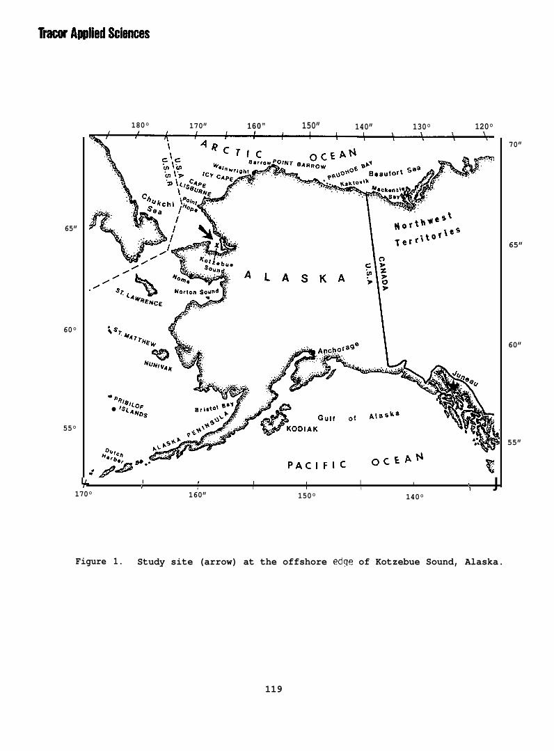
Our camp was located on landfast ice at the entrance to Kotzebue Sound
(66° 41.1’ N, 162°55.9’ W, Fig. 1), a site about 28 km southwest of
the village of Kotzebue. The nominal thickness of ice in this region was
2 m. Snow cover was light. The area was moderately ridged, landfast
first year ice with hummocks and fractures. The bottom in this location
is flat, the depth being about 14.5 m to the top of the flat ice. The
camp was occupied from 22 March-13 April 1984. The period of 19-21 March
118
jOLIOU 2OflqJJ ) 0$4r
r V 2 K Vn.-. o.p C.,
v
OJ/ib.(U BenoL,
8yOM 9
OCE
BIAYI,cISIJx.
ee9
bVC I E I C
cbE -.53 ii c1'
0IkLOMèc
BIAYI,cISIJx.
8yOMftl ee9
65”
60°
55°
180° 170” 160” 150” 140” 130° 120°
‘-’REUCE Y \iS
-P●
9 II
I I 1 I I !
170°I I r
160”1 1
150° 140°
70”
65”
60”
55”
J
Figure 1. Study site (arrow) at the offshore edge of Kotzebue Sound, Alaska.
119
Tmcor Ap@ied Sciences
was spent assembling snowmachines, readying the field instrumentation,
and locating ringed seals. The latter task, of considerable importance
to the project, was undertaken by J. Burns (Alaska Department of Fish and
Game), B. Kelly (University of Alaska) and associates working with
trained dogs. Within a 5.6 km radius of camp, 21 locations were marked
signifying breathing holes, and active or abandoned lairs.
Transportation and shipping to and from the base of our operations at
Kotzebue were furnished by a NOAA helicopter and crew. Snowmachines were
used for local transportation of personnel and gear near the study site,
although we also walked long distances to minimize disturbance to the
seals.
B. Sensors, Telemetry, Sound Speed
Underwater sound was received with hydrophores (Milcoxon H-505,
InterOcean R-130, and sonobuoys AN/SQQ-57A) placed through holes drilled
in the ice. PVC pipe casings and antifreeze were used to prevent loss of
the Wilcoxon hydrophores due to freezing. Besides being an antifreeze
mechanism, the pipe casings also isolated the hydrophore cable from
vibrations due to stress relief (cracking) in the ice. These vibrations
can interfere with measurements if the ice is allowed to freeze around
the cable. The InterOcean hydrophores were used while being attended,
thus they were recoverable. However, the sonobuoy sensing units and
cables had to be sacrificed.
When certain of the measurements were made at frequencies greater
than 15 I(Hz, a portable recorder (Nagra 4-SJ) was connected directly to
the hydrophore and a portable, wideband amplifier in the field. One
recording channel was “hard-wired” to a hydrophore via coaxial cable.
Appropriate amplifiers and line drivers were provided to prevent signal
loss, and the entire system was calibrated as a unit. For other work,
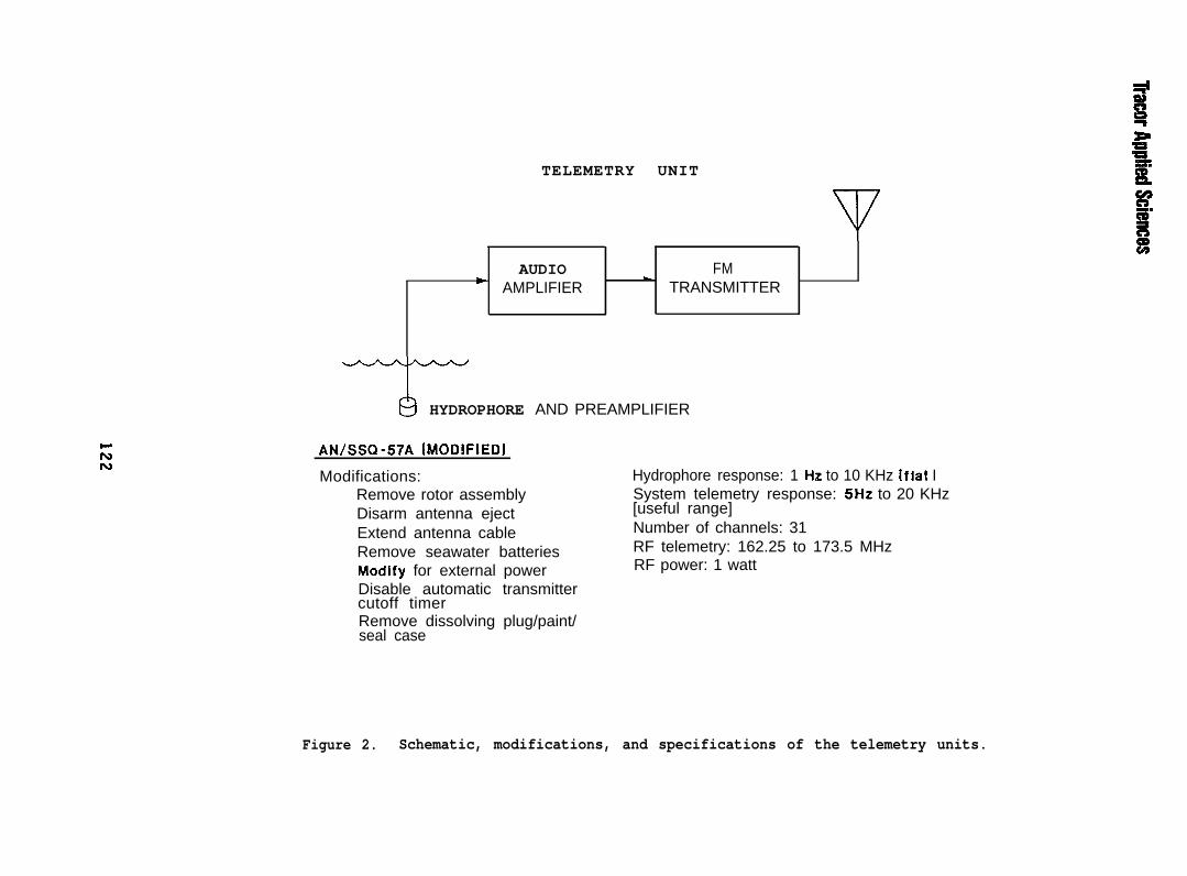
telemetry was provided by transmitters from modified AN/SQQ-57A sono-
buoys . Considerable modification of these sonobuoys was necessary in
order to dismantle the normal air eject mode, provide for long-term
120
TmcoII AIIvIMI Sciences
operation with large (105 amp/hr) 12V storage batteries, and provide for
additional matched, variable gain amplification (Fig. 2). Just prior to
the field work, all three types of hydrophores were calibrated at the
U.S. Navy calibration facility in San Diego (TRANSDEC). The design of
the instrument was such that these calibrations would not be expected to
change due to water temperature changes between this facility and
Kotzebue. All of the instrumentation exposed to outside temperatures was
tested in a laboratory freezer during the period of preparation.
Three of the hydrophores were installed in a triangular array set up
about 1 nm SW of our camp (Fig. 3). These were designated hydrophores A,
B, and C, their separation being 118.9, 99, and 108.2 m, respectively.
Hydrophore A, installed through a pipe casing, was cable-connected to our
camp, a distance of 1.8 km. B and C (sonobuoys) were received at the camp
by radio telemetry. Another sonobuoy (D) was installed about 3.7 km SW of
the triangular hydrophore array. About 2.8 km NW of the triangular array,
a bearded seal pup was found in an active lair consisting of a natural
opening between ice blocks. The animal was identified byJ. Burns. Here
we installed a sonobuoy hydrophore as a microphone, above the water’s
surface. This location was designated as E, the “bearded seal lair”.
A sixth sonobuoy (F) was used as a microphone in an active lair about
1.4 km NW of the camp. A seventh sonobuoy (G) was installed about 5.6 km
N of the camp and 25 m from an access hole that was being used by a
ringed seal and its pup. There was no den at G, and the seal hole was
made through a refrozen fracture. We located this hole and two others in
the general vicinity simply by scanning the area with binoculars on a
comparatively warm, bright, sunny day. This fracture extended for miles
and contained numerous breathing and access holes. The eighth recording
location (H) was situated 192 km W of Kotzebue. Here we drilled a 1 m
hole through a refrozen polynya and deployed a cable-connected InterOcean
hydrophore for two recording sessions lasting two hours. This far off-
shore site was an area of active ice. It was not possible to record
there for a longer period because of the environmental limitations placed
upon both airplane and personnel. Locations of all recording and
playback sites are summarized in Fig. 3.
121
TELEMETRY UNIT
gq
AUDIO FM> \
AMPLIFIER TRANSMITTER
43 HYDROPHORE AND PREAMPLIFIER
AN/SSQ-57A IMOD!FIEDI
Modifications: Hydrophore response: 1 Hz to 10 KHz [flat IRemove rotor assembly System telemetry response: 5Hz to 20 KHzDisarm antenna eject [useful range]
Extend antenna cable Number of channels: 31
Remove seawater batteries RF telemetry: 162.25 to 173.5 MHz
Modify for external power RF power: 1 watt
Disable automatic transmittercutoff timerRemove dissolving plug/paint/seal case
Figure 2. Schematic, modifications, and specifications of the telemetry units.
lhwor Applied Sciencest
OHoD
Q---q\ ,/ \\\ \\ /’ \
G)@
OF
m
oE
oG
DISTANCE DIRECTIONSITE FROM CAMP [MAGNETIC]
A 1.8 krn 238°
B 1.9 k m 237°
c 1.9 km 240°
D 5.7 km 2390E 4.8 km 260°F 1.4 km 281°
G 5.6 km 353°H 192.0 km 296°
Figure 3. Sketch of recording site layout with distances and directionsfrom camp (drawing not to scale).
123
Tmtwr AwIIM Scbnces
Supporting data collected during the period of field work included
measurements of windspeed and direction, air temperature, light, and
unde~water sound speed profiles.
c. Recordinq
To allow for seal location, site preparation, and dismantling, the
actual data recordings and sound playback took place 25 March to 11 April
1984. During this period of time 209 hrs were recorded from the tri-
angular array on magnetic tape, most of which included sounds from all
three hydrophores recorded simultaneously. In other words, one hour of
recording from the triangular array may have consisted of 1 to 3 channels,
usually 3. In addition, there were 36 hrs of recordings from the other
sensors (D-H) for a total of 245 hrs (Fig. 4). Recordings for long-term
monitoring and localization were made with a 4-channel instrumentation
recorder (Nagra T). Some long-term monitoring from the remote sensors
was also done with uncalibrated recorders (GE, Mod. 3-5105F) for the
purpose of determining the frequency of occurrence of sound production.
Short-term calibrated recordings were made with a 3-channel instrumenta-
tion recorder (Nagra 4-SJ).
D. Playback
A series of playback sessions was undertaken in the area of the
triangular array. The underwater sound projector (Navy Type J-9) was
lowered to half depth through a large hole chiseled through 2 m of ice at
a location 26.2 m from A and 99.5 m from C (Fig. 5). Peak source levels
were 135 to 140 dB re 1 pPa, 1 m. Dimensions of the ice opening were
0.75 x 1 m.
Playback data were rerecorded from field recordings taken in prior
years, in addition to alternating random noise and a 1 kHz tone. We used
a 25-rein continuous series of Vibroseis sweeps alternated with 14 min of
noise associated with Vibroseis operations (operating bulldozer, drilling,
Figure 5 . Orientation of the playback location (star) in relation to thetriangular array of hydrophores. Surface topography (ridges, refrozenfractures, etc.) as reconstructed from surface measurements and aerialphotographs is stippled. Heaviest stippling indicates surface relief ofabout 2 to 3 m.
126
Tmor Applied Sciences
movement of heavy track vehicles
also used 40 min of random noise
and personnel, etc.), Figs. 6 and 7. We
alternated with 45 min of 1 kHz tones.
Ten minute silent control periods were allowed between adjacent playback
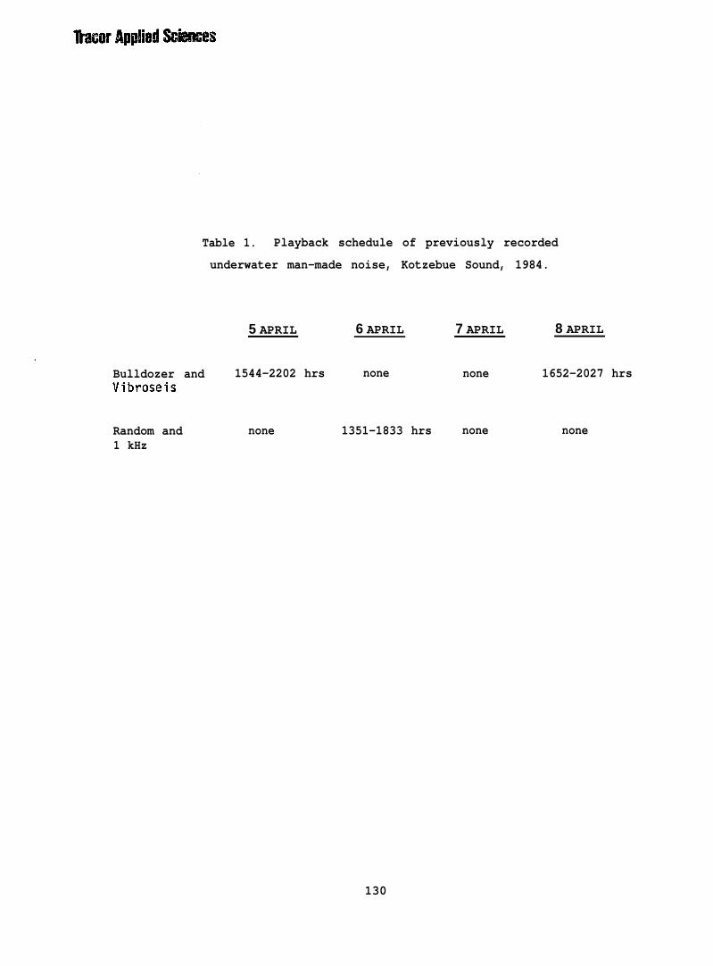
sessions. The total duration of playbacks was 14 hrs, 35 rein, scheduled
as shown in Table 1, with inclusive short, silent control periods.
Playbacks were undertaken on 5, 6 and 8 April, with portions of the
recordings at other times being used as controls. Continuous recording
was underway during both playback and the interspersed silent control
periods. The experimental design was to allow time for recordings of
ringed seal sounds before and after playbacks.
E. Analysis
Five basic types of analysis were utilized in this study: 1) waveform
and spectrum analyses, 2) determination of the rates of sound production
(frequencY of occurrence), 3) correlation, 4) sound localization, and 5)source level determination.
Waveform Analysis
Individual vocalizations or other sounds can be characterized by
duration (time), level (power), and frequency (analogous to pitch). The
last two parameters often change within an individual vocalization, and
the first may be variable between sounds.
It is useful to convey the characteristics of a sound by plotting
sound pressure level or some proportional quantity, such as a voltage
from a pressure sensor, versus time, a technique that primarily utilizes
the time domain. This type of display (Fig. 8) conveys at a glance theduration and complexity of a waveform in terms of level and frequency
over the sound’s duration. A close examination will reveal average and
peak pressure levels, and variations (if any) of level and frequency.
127
Lllzi=
o I I Io 1000 2 0 0 0
FREQUENCY [l-h]
Figure 6. Waterfall display (time history) of Vibroseis and associated industrialnoise playback, recorded on the triangular array, showinq the fundamental and UD
to the llth harmonic, analyzing filter bandwidth, 7.5 Hz.
roe isi.
F'
Tracer Applied Sciences
u,!>
i=a-1
:
!5i=a-1wK
F------ LIN X HZ
*
5K
43 LIN x w 1=
SPL = Sound pre~~ure Level
F i g u r e 7 . I n s t a n t a n e o u s s p e c t r a (upper) a n d 1 5 s e c d u r a t i o no f p e a k h o l d s p e c t r a ( l o w e r ) o f s e i s m i c e x p l o r a t i o n c o n v o ynoise playback consisting of D-6 cat scrapinq ice, drill,and trucks. Analyzing filter bandwidth 18.8 Hz and 37.5-Hz,respectively.
Table 1. Playback schedule of previously recorded
underwater man-made noise, Kotzebue Sound, 1984.
5 APRIL 6 APRIL 7 APRIL 8 APRIL
Bulldozer and 1544-2202 hrs none none 1652-2027 hrsVibroseis
Random and none 1351-1833 hrs none none1 kHz
130
I.
Tmcor A@ied Scknces10.0
0.0
-10.0
1 t 1 I, 1 t t,
w -[
t, 1r
I II
I 1,
I
0.0 0.4 0.8TIME (SEC)
10.0
I
I 1 I t ! #, I
-1.
0.0-
-10.0 1 ! I1 I I [ I0.00 0.02
TIME (SEC)0.04
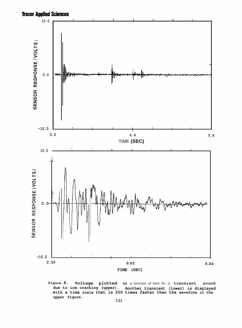
Figure 8. Voltage plotted as a function of time for a transient sounddue to ice cracking (upper). Another transient (lower) is displayedwith a time scale that is 200 times faster than the waveform in theupper figure.
131
Ikatmr A19PIW Sckmces
Some sounds consist of multiple parts separated ~
example appears in Fig. 8 (upper), where the voltage
plotted versus time. The sound was ice cracking, a [
n time. Such an
from a hydrophore is
ommon Arctic sound
of stress relief produced by differential expansion and contraction of
ice with ambient temperature changes. Four distinct arrivals of this
sound and several less intense events are displayed. Peak and average
pressure levels are calculated by means of calibration between voltage
and sound pressure. Sound pressure level decreases after the initial
transient for each of the four large signals. These sounds are described
as pulses with sharp leading edges and exponentially decaying trailing
edges or “tails”.
Expanding the time base reveals additional detail in the pressure-
time history of a sound (Fig. 8, lower). The signal envelope builds
quickly to a peak and then decays relatively slowly over a total time of
about 30 ms (milliseconds). The times at which the voltage (pressure) is
zero are zero-crossings. If these are evenly spaced in time, the signal
is defined as “narrowband”, otherwise it is “broadband”. Narrowband
signals have a restricted frequency range. Wideband signals, including
many transients, contain many different frequencies.
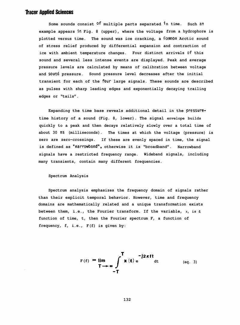
Spectrum Analysis
Spectrum analysis emphasizes the frequency domain of signals rather
than their explicit temporal behavior. However, time and frequencydomains are mathematically related and a unique transformation exists
between them, i.e., the Fourier transform. If the variable, X, is a
function of time, t, then the Fourier spectrum F, a function of
frequency, f, i.e., F(f) is given by:
rT() -j2xftF(f) = Iim x t e dt (eq. 3)
132
1-0.00(t) =0W E
5IE(t)151
Tracar Ap@ied Sciences
We often use the power spectral density,which is defined as:
Here E represents the expectation operator and
(f), of the waveform x(t)
(eq. 4)
must be invoked only in
the event the signal has a stochastic component. The symbol T represents
time. As in most analyses done on modern computer systems, we implement
these functions with the Fast Fourier Transform (FFT) algorithm (also see
Bendat and Piersol, 1966; Otnes and Enochson, 1972; Anderson, 1971, and
Middleton, 1960).
The power spectral density of an ice-cracking transient is displayed
in Fig. 9. The curve represents the power in a 1 Hz (Hertz) band at
frequencies over the analysis range, here 2 kHz. The power is distrib-
uted widely over the band, with maxima at about 10 Hz and near 900 Hz.
Spectrum levels are approximately -43 dB for each peak. This electrical
power spectral level corresponds, through the calibration constants for
the measurement system, to a sound pressure spectrum level of 79dB re
1 uPa in the water.
Sound Frequency of Occurrence
One of our objectives was to report any differences in sound frequency
occurrence over time. If present, such a trend may be a means of infer-
ring changes in behavior. Many animals exhibit diurnal patterns in activ-.ity that are often indications of related behavior. Sound production isalso known to be part of the reproductive behavior in many species. Our
field period was explicitly chosen by the sponsor to begin before the
pupping season for the ringed seal and to end after the season was well
underway.
133
-7-7
I00
00
0z
*u)
z1-
Cu0)
II
II
II
I
el
●
-0csWI
0
al>.m
134
In view of these and other possible temporal dependencies, we moni-
tored all recordings, logging each occurrence of animal sound by type and
accumulating totals in fifteen-minute periods. These data were then
stored in a computer file for subsequent analysis, e.g., the frequency of
occurrence for barks, scratches, squeaks, rubs, etc. The total numbers
of animal sounds were also accumulated and plotted. Names of sound cate-
gories were mostly derived from their aural appearance, i.e., rub, quack-
ing bark, etc., which does not imply the mechanism of sound production.——
Correlations
Correlation analyses between environmental measurements and rates of
sound production were undertaken using two techniques, graphical means
and statistical calculation. For example, we calculated simple regression
equations and coefficients of determination, and we applied the chi-
squared and Student’s t tests. As explained below, cross-correlation
between two or more arrivals of the same sound was used in the localiza-
tion procedure to determine the geographical origin of sound sources.
Localization
A single, omnidirectional hydrophore can be used to detect a sound,
provided the level of the sound at the hydrophore is sufficiently high
relative to background sounds, i.e., above O dB signal-to-noise ratio. B y
itself, such a hydrophore cannot be used to determine either the distance
to the sound source or the direction from which the sound originated.
However, with two sensors of this type, separated in the horizontal plane
by a known distance, one can solve an equation to determine that the
sound came from one of two possible directions (bearings). In practice,
there usually is not sufficient information to resolve this ambiguity.However, by adding one additional hydrophore, not co-linear with the
other two, one can calculate, not only the direction to the sound source,
but also the distance.
135
lkatxw AIIIWI ~IMX!S
Our technique for doing this was developed and tested for under-ice
localization in an OCSEAP project off Prudhoe Bay in 1981. The procedure
and results are fully documented (Cummings, et al., 1981). Basically,
this involves measuring the difference in arrival times of the sound of
interest at each hydrophore, generally the same method of triangulation
as used in related disciplines, such as optical tracking.
In past efforts (also see Cummings, et al., 1983), we used the time
of the initial arrival of the sound at each hydrophore to determine the
time delay between hydrophores. This is relatively simple in the case of
sounds with sharp leading edges or ones that have propagated over similar
paths. It is considerably more difficult if the leading edge of the sound
envelope is ambiguous, or if the waveforms differ on each hydrophore due
to propagation perturbations. The optimal solution to determining the
time delay at two sensors is by cross-correlation. The cross-correlation
function, R(T), is a function of the time delay, T, between signals on
two time functions, x(t) and x(t+~). The correlation function is defined
as:
m
R(T) =J
X( t ) X(t+T)dt
-ao
The remainder of this discussion utilizes a transient sound from
cracking ice recorded on our triangular hydrophore array to illustrate
{eq. 5)
the localization procedure. The identical
localize the animal sounds
Three hydrophores (ales”
1.8 km from the ice camp.
gnated A, B, C)
The geometry of
procedure was employed to
were positioned at a location
the hydrophore locations and
the surrounding ridge and refrozen fracture structure are illustrated in
Fig. 10. The hydrophores were all located at a depth of 8 m from the icesurface in 14 m of water under 2 m of ice. The hydrophore signal from
location A was transmitted, after amplification near the site, via a
136
I“ Applied Sciences
1829m coaxial cable (RG-174/U). Signals from hydrophores at locations B
and C were telemetered to the ice camp, and all three sensor outputs were
recorded simultaneously on a Nagra T recorder.
Plots of the voltage at hydrophores A and C (Fig. 11, upper) reveal
that the signal at hydrophore C arrived about 72 ms later than at hydro-
phore A (AAC). Because of slight differences in propagation path losses
and ambient noise, it is very difficult to measure the delay more accu-
rately from this type display. The mathematically optimal manner for
obtaining a more accurate estimate of the delay between the two signals
is to compute the cross-correlation function (eq. 5). The result of that
calculation (Fig. 11, lower) is a waveform with a distinct peak at the
delay between the two signals, 72.27 ms. In the firmware implementation
of the cross-correlator, provision is made to set a cursor on the peak,
providing a direct digital display of the delay. A similar measurement
of the delay between the sound arriving at hydrophores A and B resulted
in AAB = 52.93 ms.
A computer algorithm was used to calculate the parabolic curve
labeled AAB = +52.93 ms in Fig. 10. This was based on an average
measured sound speed of 1437 ~ 1 m/see. A sound originating at any
position on this curve would arrive at hydrophore B, 52.93 ms later than
at A. Similarly, the curve labeled AAC = 72.27 ms represents the locus
of points from which a sound would reach hydrophore C, 72.27 ms later
than at A. The intersection of these two curves is the location of the
ice cracking sound. The coordinates, with respect to hydrophore A, are
x = 218.2 m and y = -126.1 m. This corresponds to a range of R = 252 m
and a bearing of EI= 240° , relative to location A and line A-B. There-
fore, this particular sound originated on a discontinuous, linear ice
ridge with relatively low, ca 1 m, relief (Fig. 10).
This procedure was used to localize additional ice-related sounds and
a number of animal sounds. Our objective was principally to obtain a
distance to the source of the sound in order to determine its source
F i g u r e 1 0 . S e n s o r l o c a t i o n s ( A , B , C ) , i c e ridges ( s t i p p l e d ) , t r i a n g u l a ra r r a y , a n d t h e i n t e r s e c t i o n o f t w o p a r a b o l a s ( s t a r ) b a s e d o n thei n d i c a t e d s o u n d a r r i v a l t i m e d i f f e r e n c e s .
138
HADBObHOI4E V
IILLI I.. -
HADBObHOIIE
Ti’acor AppMed Sciences1 I
,1 I t
,1 I
I,
1
_ - - 1 I + AAC “ +72.27 ms
JIL
HYDROPHORE C
//I~m
, II
! I I 1 I I I 1 J0.0 0.2 0.4
I 1,I
T ‘ + 72.27 MS —
[ 1 It I
#11
-0.2 0.0 0.2
TIME (SEC)
Figure 11. Arrivals of the same ice cracking transient sound athydrophores A and C (upper) and their cross correlation functionused to determine the arrival time difference, 72.27 ms (lower).
139
Tmcor Applied Sciences
level in dB at a standard distance from the point of origin. Also, we
wanted to look for any spatial clustering or association with ice surface
features.
Source Level Determination
We define s o u r c e l e v e l a s t h e m e a s u r e o f t h e l e v e l o r i n t e n s i t y o f a
s o u n d . This quantity is defined as 10 times the common logarithm of the
ratio of the intensity of the source, on its acoustic axis (if any), to
the intensity of a plane wave with a root mean square pressure of one
micropascal (~Pa), referenced at a distance of 1 m from the source.
An absolute measure of the sound intensity at a known distance is
required to measure source level. To our knowledge, th i s measurement has
not been done in the case of pinnipeds in the wild. Knowledge of source
level (SL, eq. 1) is required to quantify potential masking or other
impact on a species from the addition of man-made noise to the environ-
ment. Thus, we carefully calibrated the instrumentation used to localize
sounds with the triangular array of hydrophores.
140
Tmcor Applied Sc@ms
v. RESULTS
A.
one
Ringed Seal Sounds
A total of 24,373 individual animal sounds was recorded. Except for
bearded seal pup in a lair (location E), ringed seals were the only
pinnipeds seen in the study area. It is possible that a small portion of
the vocalizations could have been from bearded seals, based on the fact
that some very weak bearded seal trills were heard over two days during
our recordings in the Sound. They were powerful and numerous on the off-
shore recording, 192 km distance.
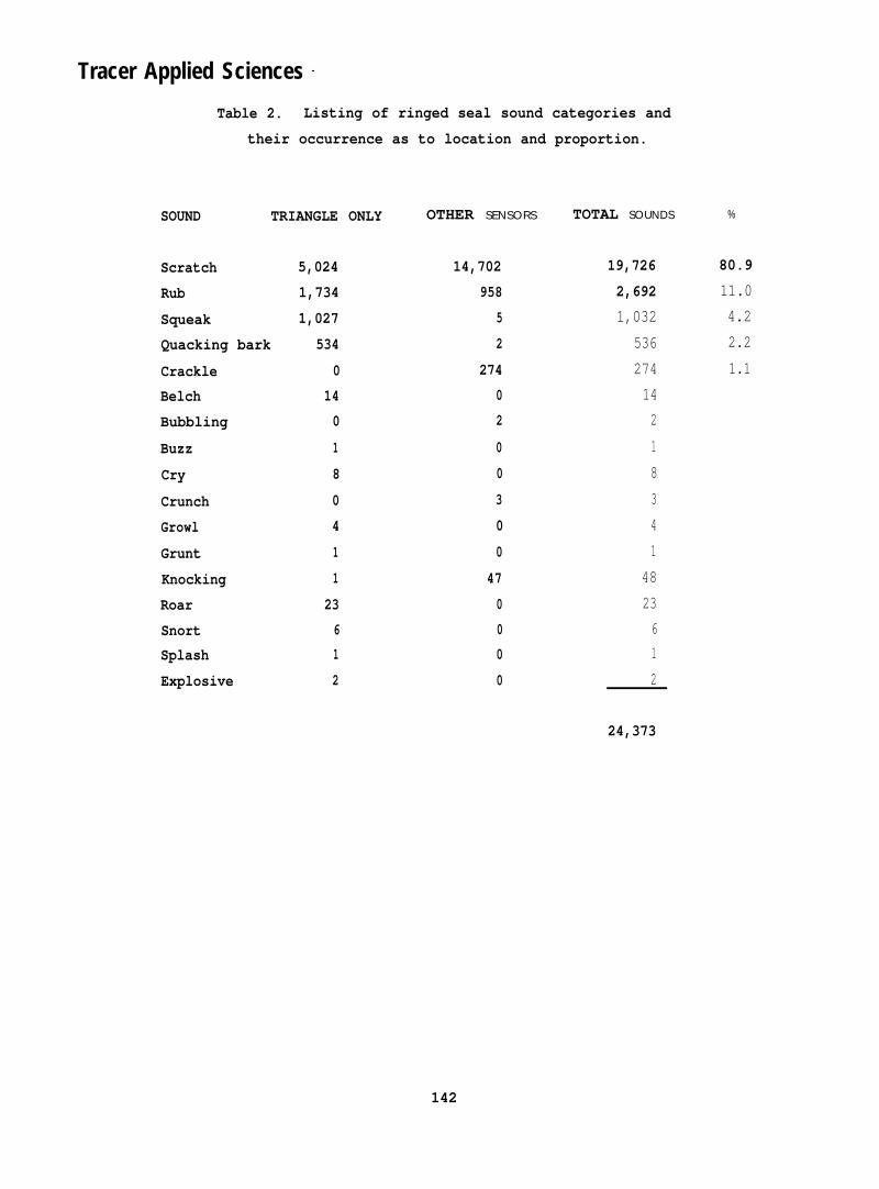
We recognized 16 different categories of seal sounds. Most of the
recorded sounds were scratches that were produced as the seals either
clawed at their access or breathing holes to maintain the openings in the
i c e , o r m a i n t a i n e d t h e i r l a i r s . E l e v e n p e r c e n t w e r e r u b s o u n d s . N o t
c o n s i d e r i n g s c r a t c h i n g s o u n d s , r u b s w e r e t h e m o s t c o m m o n o f t h o s e s o u n d s
t h o u g h t t o b e p r o d u c e d a s v o c a l i z a t i o n s . A t o t a l o f 4 . 2 % o f t h e s o u n d s
w e r e s q u e a k s . Quacking barks accounted for only 3.2% of the sounds, but
they were outstanding vocalizations when present. Crackles were 1.1% of
the total. A listing of the sound categories, including their percentage
of occurrence, appears in Table 2.
Although totals are given for the three hydrophores comprising the
triangular array and we frequently heard the same sound there on all
three sensors, each occurrence was only counted once in these tabula-
tions. About 70 percent of all the scratches came from location E where
we had installed a hydrophore in an active lair that was occupied by a
bearded seal pup and, presumably, an attending adult. Infrequent sounds,
for which the percentage of occurrence is not given in Table 2, together
amounted to 0.6% of the total number of seal sounds. Only the common
sound categories are included in the following descriptions.
141
Tracer Applied Sciences ~
Table 2. Listing of ringed seal sound categories and
their occurrence as to location and proportion.
SOUND TRIANGLE ONLY
Scratch
Rub
Squeak
Quacking bark
Crackle
Belch
Bubbling
Buzz
Cry
Crunch
Growl
Grunt
Knocking
Roar
SnortSplash
Explosive
5,024
1,734
1,027
534
0
14
0
1
8
0
4
1
1
23
61
2
OTHER SENSORS
14,702
958
5
2
274
0
2
0
0
3
0
0
47
0
0
0
0
TOTAL SOUNDS %
19,726 80.9
2,692 11.0
1,032 4.2
536 2.2
274 1.1
14
2
1
8
3
4
1
48
23
6
1
2
24,373
142
Trawr Applied Sdences
Scratches
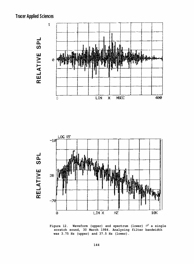
We recorded a total of 19,726 scratches, representing 81% of all seal
sounds recorded during the study period. Scratching sounds typically
were 40-500 msec in duration (Fig. 12, upper) with peak frequencies of
1000-6000 Hz (Fig. 12, lower). Nearby scratching sounds, that were less
affected by high frequency attenuation losses, contained energy up to
10 kliz, but for the most part the recorded sounds were below 6 kHz. The
high frequency content and the peak frequency usually decreased over the
duration of each scratch (Fig. 13). S c r a t c h e s w e r e a s e r i e s o f b r o a d b a n d
t r a n s i e n t s t h a t o c c u r r e d a t i n t e r v a l s o f 4 0 0 - 6 0 0 m s e c ( F i g s . 1 4 , 1 5 ) .
Aural characteristics were like strokes of sandpaper across a hard sur-
face. Source spectrum’ levels for two scratches are given in Figs. 16 and
17. Peak source spectrum level was 102 dB re 1 ~Pa, 1 m, for one and
98 dB for the other. A detailed analysis was done of the occurrence of
these sounds (see B., Frequency of Occurrence, Scratches, below).
Rubs
A total of 2,692 rub sounds was recorded during the study. This
represented 58% of all the vocalizations recorded at the array (excluding
scratches). Rubs were the most common of all ringed seal vocalizations.
We recorded as many as 239 rub sounds in 8 hrs of recording and as many
as 92 in 15 rein, i.e., 9 April. This description was used because the
sound so clearly resembled the rubbing of one’s wet finger tips over a
shiny hard surface, such as glass or the waxed surface of an automobile.
Peak sound pressures of rub sounds occurred between 0.5 and 2 kHz, with
most of the sounds’ energy below 4 kHz (Figs. 18 and 19). The waveform
of one rubbing sound and the cross-correlation are shown in Fig. 20.
Durations of rub sounds fell in the interval from 80-300 ms, and the peak
source spectrum level was about 95 dB re 1 uPa (Fig. 21).
143
roe L.L
DB
Tracer Applied Sciences
0 LIN X MSEC 44*
Figure 12. Waveform (upper) and spectrum (lower) OF a singlescratch sound, 30 March 1984. Analyzing filter bandwidthwas 3.75 Hz (upper) and 37.5 Hz (lower).
Figure 19. Ambient spectrum (upper) and the additive spectraof 12 rubs (lower) showing most of the energy is in thefirst 2 kHz with the peak at about 1 kHz, analyzing filterbandwidth, 7.5 Hz.
151
BflB
Tmcor Applied Sciences1
0
-11
0
-1
0 0.4 0.8
TIME (SEC)
+1
o
-1
RUB
o
Figure 20.A and C,functionbe 46.88
. 0.8
TIM; ~SEC)
Waveforms of the arrivals of a rub sound at hydrophoresin the triangular array (upper) and the cross correlationof same (lower) showing the arrival time difference toms.
mulfDsq2'uo2.Ibrluo2eIIT.V61'Th16[LJfl6
.H2.8IrLbwbnbd
Tncor Applied SciencesII
II
I—
m
0
u)10a“Q
- “mOuo
153
Tmcor Arplied Sciences
Squeaks
These sounds, recorded 1,032 times, were the second most common
vocalization (excluding scratches). This represented 4.2% of all sounds
or 22.2% of vocalization. Aurally, squeaks were like rubs but generally
shorter in duration and higher in frequency. Spectra for two squeaks are
given in Fig. 22.
The source spectrum level ofa squeak is given in Fig. 23. This sound
peaked at 112 dB re 1 pPa, 1 m.
Quacking Barks
Quacking bark sounds strongly resembled vocalizations of ducks. They
accounted for 2.2% of the total number of sounds recorded from ringed
seals at the triangular array, or 11.5% of the vocalizations (excluding
scratches). These sounds normally were produced in volleys of two to
five sounds. The waveforms and cross correlation function of a two-
element quacking bark appear in Fig. 24. Durations ranged from 30-120 ms
with the peak frequencies occurring at 400-1500 Hz. Components of
quacking bark sounds were found up to 5 kHz, but most of the energy was
less than 2 kHz. The fundamental frequency was typically at about 90 Hz
(Figs. 25- 27). A good example of how the propagation path can affect
the spectrum of sounds appears in Fig. 27, lower, where the energy at
0.2 kHz is subdued as received from hydrophore A, compared to C. The
source spectrum level of a quacking bark is given in Fig. 28. It peaked
at 130 dB re 1 vPa, 1 m.
B. Frequency of Occurrence
Long-term (triangle)
Based on a histogram of the frequency of occurrence of recorded ringed
seal vocalizations at the triangle, excluding scratches, the rate of
sound production increased over the period of our recordings (Fig. 29).
154
DB
-
5
Tmcor Applied Sciences
UJG w.
0 LIN X HZ UzlKx
UIG la,
m
,
$? MN x !-z 143(x
Figure 22. Spectra of a high S/N ratio squeak (upper) andOfle Of 10W S/N (lower), analy.zi~q $ilter bandwidth, 37.5 Hz.
155
Tncor Applied Sciences
oOA
II
I1
II
o0o1-
U)qN00co
..-
w-L
BV8KOflYCKII1C
1 II 1 I
I1 I, I
I1
11
+
o
-11
0
-1
0 0.2 0.4TIME (SEC).—– —,
+1
It I I 1 I I
II1
QUACKING BARK
t
1 I ! I1
0 0.2 0.4
TIME (SEC)Figure 24. Waveforms of the arrivals of a two-element quacking bark
sound at two hydrophores in the triangular array (upper) and thecross correlation function of same (lower) showing the arrivaltime difference to be 8.98 ms.
.,:
'1r r
-TO
iii jf.1 czi.
it- MIIN
DB
Applied Sciences
z
-J 43nto
0 LIN X WC.
F LOG RT
a-1wK
0 LIN X l+? 2K
Jamu)
;1-a-1
Ii!
mm
# LIN X HZ %
Fiqure 25. Waveform and spectrum of a sinqle quackinq bark (upper),;nd the same of another quacking bark (l;wer), stre~chinq out thetime scale for more detail of the waveform. Analyzing filter band-width, 7.5 Hz (above), 18.75 Hz (below).
158
DR
Tracer Applied Sckncesl_QGMt
I@ 1
IM I IImk n , i f
43 I-m x Hz %
-1ato
w>L4JLLlu
UK hit
0 LIN X I-G! 5?(
Figure 26. Addition of peak spectra over eight consecutivequacking barks (upper) and the exponential average of thesame (lower). Duration, 3.09 see, analyzing filter band-width, 18.75 Hz.
159
tab)
YT
II43O
MU
RT
O2
Hw
oI
II
II
II
II
I
('1c
41%
)C
O-
c4
roC
o0
00
00
0000
00
00
0
DB
HADBObHOIIE C
HADBObHOIIE V
Tmcor Applied Sciences
0 0.5 1.0
FREQUENCY (kHz)
Figure 27. SDectrum of a single quacking bark analyzed at peak amrJlitude(upper), analyzing filter bandwidth, 18.75 Hz. Power spectral densities(O-1 kHz) of the arrival of a quacking bark at two hydrophores in the tri-angular array, analyzing filter bandwidth, 3.7 Hz.
160
1
II
Ia
CA
IT m 0 rn1
C)
>. I fri
Tncor Applied Sciences
.
●
✍
161
I
G0
Co
G0
V co1692b9pnhoJipnibiooeiSI1ZI19V0be15m1on919WLt6b
to be a rapid increase in sound production beginning
It was necessary to normalize these data because of
unequal recording effort between days. The data were analyzed by counting
the number of all vocalizations from the triangular array in all cate-
gories per hour of recording in each day, and extrapolating by multiply-
ing the average number of sounds per hour by 24, the hours in each day
represented.
The long-term occurrences of the most prominent and frequent ringed
seal sounds are shown in Figs. 30 and 31. The increase in sound produc-
tion (bar heights, not numbers of bars) can readily be seen in the case
of rubs, squeaks, and barks; however, the occurrence of scratches appeared
to diminish over the recording period (Fig. 31, lower). These data were
normalized for unequal recording durations since they were plotted as the
number of sounds/hr. The total numbers of sounds, including scratches,
were also plotted as a histogram in terms of sounds/hr, but the trend
toward increasing sound production rates was obscured by the pattern of
scratch occurrences (Fig. 32).
The occurrences of ten other sound categories recorded from the
triangle were plotted as histograms using the computerized file of their
counts, but the total numbers of sounds were too low and infrequent to
depict as histograms. Instead, these infrequent ringed seal sound cate-
gories are tabulated (Table 3). This table can be referenced for the
relative total frequency of occurrence for these sounds.
Long-term (other sensors, D, E, F, G)
The occurrence of ringed seal Sounds at the remote hydrophores
generally was too infrequent to detect long-term changes. A single
exception was the occurrence of scratches at E, discussed below under
“Scratches”. These hydrophores were installed and disassembled at random
times over the entire recording period of 25 March-n April. If one of
them ceased to function, or the bioacoustic activity was nil for 24 hrs
or more, we discontinued the station. Usable sensors were sometimes
moved to other locations where we noted activity, e.g., to location G
where a ringed seal mother and pup were spotted sunning themselves near a
newly opened access hole in a refrozen fracture.
163
Tracer Applied Sciences140
120
100
80
60
40
20
0
160
140
120
100
80
60
40
20
0
RUBS
10 ! II36 87 88 89 90 91 92 93 94 9S 9
DAY
SQUEAKS
L101
I
I L, IJ.. ill, ,1I
II I
86 87 88 89 90 91 92 93 94 95 96 97 98 99 10010
. 12.
DAY
Figure 30. Histograms showing the long-term increase in the rate of rub(upper) and squeak (lower) sounds from rinqed seals over the recordinqperiod beginning with Julian day 86 (26 March 1984). Periods marked byunderlying bars were not recorded.
Figure 31. Histograms showing the long-term occurrence of ringed seal soundproduction rates of quacking barks (upper) and scratches (lower) over therecording period beginning with Julian day 86 (26 March 1984). Periodsmarked by underlying bars were not recorded.
Table 3. Occurrence of infrequent ringed seal vocalization
categories from the
SOUNDCATEGORY “
Cries
Belches
Roar
Buzz
Knocking
Splash
Grunt
Snort
Explosive
Growl
lDenotes number of soundswhich there was at least
triangular array period, 25 Mar-17 Apr 1984.
DATES OFOCCURRENCE, ’84
27 Mar
30 Mar
31 Mar
6 Apr
9 Apr
3 Apr
29 Mar
9 Apr
28 Mar
30 Mar
30 Mar
17 Apr
NUMBER OF SOUNDSPER HOUR1
8
1
8
4
22
1
1
1
1
4
1, 3, 1
‘4
that occurred during a recorded hour overone occurrence.
167
Tmcor ApPlid Sciences
The occurrences of six different sound categories are listed in
Table 4 according to remote hydrophore locations D-G (also see Fig. 3).
With the exception of 14,702 scratches (14,589 of which came from
location E) and 597 rubs (location E), relatively few sounds were
recorded from these other hydrophores outside of the triangular array.
Diurnal (triangle)
The data were searched for evidence of diurnal (daily) patterns of
ringed seal sound production. This was done mostly by studying the
frequency of sound occurrence plots resulting from data recorded at the
triangular array of hydrophores. First, we pooled all of the sound
categories [scratches included), adding all occurrences during recorded
hours over a 24 hr period. Since the recording level of effort varied
between hours of the day (comparing day to day), it was necessary to
normalize summed data by dividing the total number of sounds by the
number of days for which a given hour was recorded. The results
(Fig. 33) suggested a bimodal distribution peaked at about 1100 and
0130 hrs.
We then searched the frequencies per category and determined that the
bimodality, or apparent diurnal periodicity, was basically due to the
occurrence of scratches (Fig. 34). In both Figs. 33 and 34, the lower
distributions are smoothed versions of the upper distributions obtained
by a moving average of 3. The occurrence of scratches peaked at 1030 and
2330 hrs (Fig. 34, lower).
Fig. 35 resulted from removing the scratching sounds and plotting the
pooled data for vocalizations. Although it appears that the frequency ofoccurrence of seal vocalizations may be independent of the hour of the
24-hr day (averaged data for the triangular array), a statistical analysis
showed there was some dependency (chi square = 38.8 > 35.2 (.05) 23 deg
freedom). In the same way the raw data showed dependence (chi square =
127.95 > 35.17 (.05) 23 deg freedom).
168
Tncor Applied Sches
Table 4. Occurrence of ringed seal sounds at sensors other than
from the triangular array during the recording period,
25 March-n April 84.
SOUND NO. SOUNDS RESPECTIVESENSOR CATEGORY PER I-IR1 DATES (J]
D Rubs 2,3 86,88II Scratches 2 - ” 88
E Rubs 114,83,400 89,89,89II Scratches See Fig. 38II Squeaks 1,1,1,2 88,89,8!?,93II Crackle 104,2 96,96II Crunch 3 9311 Knocking 9,9,2,8,21 93,93,95,96,96
F Scratches 52 89
G Rubs 21,13 96,96II Scratches 59 9611 Crackle 120,43,3 95,95,96
lDenotes number of sounds that occurred durinq a recorded hour (includedare the respectively listed Julian (J) dates, next column) over which therewas at least one occurrence.
Figure 33. Histograms showing the hourly occurrence of all ringed sealsounds from the triangular array, pooled eve? the number of daysindicated and normalized for unequal numbers of recordings (upper)and the same data smoothed by a moving average of 3 (lower).
TIME OF DAY (HOURS)Figure 34. Histograms showing the hourly occurrence of all rinqed seal
scratches from the triangular array, pooled over the number of daysindicated and normalized for unequal numbers of recordings (upper)and the same data smoothed by a moving average of 3 (lower).
TIME OF DAY (HOURS)Figure 35. Histograms showing the hourly occurrence of all ringed seal
vocalizations from the triangular array, pC)Oled over the number ofdays indicated and normalized for unequal numbers of recordings (upper)and the same data smoothed by a moving average of 3 (lower).
172
Ttacur Applied Whes
A Fast. Fourier Transform (FFT) was then produced to illustrate the
frequency of occurrence (Fig. 36). This indicated possible periodicities
of 2 and about 7 hours in the occurrence of pooled data consisting of
3,359 sounds. Figs. 33 to 36 pertain only to data from the triangular
array, which were not duplicated, i.e., only the occurrences on one
hydrophore (nearly always A) entered these data even though al l three
hydrophores were recorded simultaneously.
Scratches
Since scratches were so numerous and they were associated with known
types of behavior (breathing hole, access hole, or lair building/
maintenance), a study was made of their frequency of occurrence.
Individual scratches occurred in bouts that consisted of 1-126 sounds
(mode 4; median 11). Bouts were defined as groupings of, scratches separ-
ated by at least 3 sec. The frequency of occurrence of given numbers of
individual scratches per bout is shown in Fig 37. They comprised a skewed
curve that appears to have three peaks centered on 4, 11, and 27 sounds
per bout. By far the commonest number of scratches per bout was 6 or
less.
A total of 310 bouts was recorded from the triangular array, 26 March
to 11 April. Single bouts from a single seal lasted as long as 101 see,
and as many as 34 bouts from more than one seal occurred over a period of
2 hrs. Although only one bout may have been heard in a given time period,
bouts generally occurred in series (one group of scratches after another)
with a long pause, e.g., 1 rein, between series. We never heard scratch-
ing from two locations at the same time, although on 26 March, a series
from one location was immediately followed by another elsewhere.
On 29 March, we started to record from site E where a hydrophore had
been buried in snow and ice at the periphery of an active lair. The lair
contained a seal pup which, surprisingly, turned out to be a bearded seal
(identified by John Burns, Alaska Department of Fish and Game). The most
common sound recorded at this location was scratching. The frequency of
173
7'
mz
c)i-<N
2 5 0
2 0 0
150
100
50
01 2 6 4 3 2
PERIOD (HOURS)
Figure 36. Fast Fourier Transform (FFT) of the frequency of occurrenceof ringed seal vocalizations (sounds, excludin scratches) showing two
?possible periodicities of about 7 and 2 hours from pooled data of3,359 vocalizations at the triangle).
occurrence of these sounds was plotted over 56 hrs of recording, sampled
over 10 days, 29 March-7 April (Fig. 38). The number of scratches peaked
on the third day of recording (31 March) and then decreased until no more
were heard after 5 April. At their peak, as many as 4,388 scratches were
noted in one hour’s time, beginning at 1205 hrs, 31 March.
On 9 April, the hydrophore signal was virtually absent from locationE. The S/N ratio and the character of the noise indicated that the
useful battery power had run out. Upon our inspection of the lair and
the hydrophore, the pup was found f rozen in to the re f rozen a c c e s s h o l e
with the top of its head and back just above the surface of the ice. We
removed the transducer, battery, and transmitter. The site was inspected
on 15 April and nothing had changed.
There were very noticeable changes in the acoustical characteristics
of individual scratch sounds within bouts that presumably were caused by
scratching different
virtually all bouts,
Physical Factors
forms of ice in different ways. This occurred in
regardless of location.
and Sound Production
Four environmental factors were measured
research: ambient surface light, windspeed,
in the conduct of this
ambient air temperature, and
underwater sound speed. We measured light, wind, and temperature because
of the possibility that they may have been associated with the frequency
of occurrence of ringed seal sounds. Underwater sound speed was needed
for sound source local ization (see METHODS).
Light - The relationship of light intensity (vWatts/cm2) and time
of day was first plotted for each of 16 days, with individual datum
points at the times of measurement. As reported by the local weather
broadcasters over this period of time, daylight periods lengthened by an
average of 10 rein/day. Pooled light measurements appeared as a strong
modal curve which peaked at about 1400 hrs (local time), Fig. 39. The
176
U)
uu
23z
4800
4200
3600
3 0 0 0
2 4 0 0
1600
1200
6 0 0
0
SCRATCHES
N=14,589
89 90 91, 92 93 94 95 96 97 98H H H H lHHWH H H H H H~
DAY
Figure 38. Occurrence of scratching sounds as recorded during 56 hrs over10 days from the lair at site E, which contained a bearded seal pup, Juliandays 89 to 98 (29 March-7 April 84).
++\
If
m
800
700
600
500
400
300
200
100
02400 0600 1200 1800 2400
TINIE OF DAY
Figure 39. The total of 141 ambient light measurements vs time of day pooledover the recording time period, 25 March-10 April 84.
highest measurements varied from about 450-570 pWatts/cm2, which
occurred over the time period 0930-1800 hrs, depending upon overcast
conditions. Our photometer was sensitive enough for measurements from
about 0600-2130 hrs on the shortest day.
When the pooled sound data (excluding scratching), i.e., Fig. 35,
were divided into light vs dark hours (averaging 0600-2100, 2100-
0600 hrs), it was found that more vocalizations/hr appeared during the
light hours (chi square = 5.0> 3.8 (.05) 1 deg freedom). We have
already shown that there was some dependency of the number of seal
vocalizations/hr on time of day (Frequency of Occurrence, Diurnal).
Using the average light intensity values during times of the day (fit-
ted line, Fig. 39) and the number of seal vocalizations/15 min period that
occurred during times of measurable light, we examined the association of
the two variables. Based on 901 pairs of observations, light and numbers
of sounds were not statistically correlated (r = .014 < .062 (.05)).
Windspeed - The range, mean, and values of windspeed (mph) over 210
measurements on days of recording are given in Fig. 40. The tabulated
and graphed values, ranging from calm to 45 mph (mean 11.3, SD 9.6),
appear in the Appendix. There was a significant negative correlation
between the number of ringed seal vocalizations and windspeed, based upon
counts of sounds in the 15-min period following each windspeed measurement
(r=l-0.1851> 0.114 (.05) 210 N). In other words, more vocalizations/hr
were counted during low windspeeds. Over the above stated range of wind-
speeds, vocalizations/15-min period ranged from O to 183 (mean 8.4, SD
23.8).
The number of scratches/15-min period was not correlated with
windspeed (r = .0027 <0.114 (.05) 210 N) where scratches in the first
15-min period were counted directly after windspeed measurements. In
this set of data, the number of scratches ranged from O to 96 (mean 4.9,
SD 13.9). The range mean and standard deviation for windspeeds were the
same as those in the association with vocalizations.
179
0
8
54
35
40
48
29
94
Tncor Applied Sciences
I1
{
I
iI
}1
Ii
t{
I
Ii
tI
}
II
IiP
rI
I1
II
II
L
Temperature - The range and means of 210 temperature
readings on the days of recording are given in Fig. 41. Tabulated
temperature data, ranging from -37 to 10°C appear in the Appendix.
Temperature variations over 2 April are shown in Fig. 42. As with most
days, minima occurred during the hours of darkness, maxima at about
1330 hrs. The number of vocalizations/15-min period following each
temperature measurement was significantly negatively correlated with
temperature (r = l-0017 !z0.114 (.05) 210 N). There were more vocaliza-
tions/15-min period during lower temperatures. The range, mean, and
standard deviation for vocalization/15-min period were the same as this
comparison with windspeed since the same set of vocalization data was
used (range 0-183, mean 8.4, SD 23.8).
Because the number of vocalizations was negatively correlated with
both windspeed and temperature, we wanted to examine the association
between these two environmental factors. Using 198 pairs (recorded
simultaneously) of the two variables noted throughout the recording
period, it was determined that they were not statistically correlated
(r = .085 < 0;117 (.05) 196 deg freedom).
The number of scratches/15-min period following temperature
measurements was not significantly correlated with temperature
(r=] -O.0361 <0.114 (.05) 210 N). The range, mean, and standard
deviation of the number of scratches in this set of data were the
same as in the comparison between windspeed and scratches (O-96,
4.9, 13.9, respectively).
Underwater sound speed - A set of measurements of underwater sound
speed appears in Fig. 43. As described above, this parameter was needed
for the localization work. The values were fairly uniform from the
surface (in the ice hole and just below] to the bottom of the water
column, as would be expected in such shallow water. The average value of1437 m/see was used in the localization.
181
-00Ixl
Go.
24
16
8
0
-8
-16
-24
-32
-40
[
I
86 88 90 92 94 96 98 100 102
DAY
Figure 41. Range and means of temperature readings taken on recordingdays (N = 210).
ii!zw1-
30
20
10
0
-10
-20
- 3 0
- 4 0
- 5 0 I I I I2 400 0 6 0 0 1200 1800 2400
TIME OF DAY
000
● n●e
0°●
●
● ● m● 0
●
ao* ●
O*
Figure 42. The range of ambient temperature readings taken during 2 April 84.
Figure 43. Speed of underwater sound vs depth as measured inKotzebue Sound at the study site, 25 March 1984. The upperthree measurements were in seawater in the drilled hole.
184
Tmcar Applied Sciences
c. Other Recorded Sounds
Low frequency pulses
On more than 36 occasions during the overall recording period, a
series of low frequency pulses (LFP) was recorded. These
occurred in trains of varying total duration from 3 to 16
pulse-pulse interval was about 95 ms, and the fundamental
within a pulse was about 106 Hz (Fig. 44). The amplitude
pulses, but the received signal-to-noise ratio of a train
signals
sec. The
frequency
varied between
was typically
26 dB. The temporal onset of the pulse train was very slow vs an abrupt
off ramp.
LFP’s originated from an offshore direction, but we were unable to
localize them due to the limited size of the hydrophore array. They
appeared to be of man-made origin, but we do not know the specific source
of these curious sounds.
The onset of LFP’s was rapidly followed by a series of ringed seal
vocalizations consisting of quacking barks, squeaks and rubs on 31 of the
36 noted
and they
Water
occurrences. The vocalizations occurred during the LFP trains,
decreased when the trains stopped.
Occasionally, we recorded dripping on the water’s surface. Aurally,
the sounds closely resembled those from pouring a small amount of water
from a cup on the surface of a large volume of water. They were broad-
band sounds extending up to 10 kHz. The waveform of part of such a series
of dripping sounds and the spectrum of another appear in Figs. 45 and 46.
We have recorded these sounds before near Prudhoe Bay and Barrow.
185
n
Tmcor Applied Sciences
11
II
II
I
—–
s
‘1
-rIIII
t1
1I
I[
II
1-
U)
0u)
.F
1“I
m.N.
ld
L0EI-L
0
( S
L1
OA
) 3C
Inllld
UU
v
186
---
I
Tncor Applied Sciences
II—
iI
1I
II
II
I
o
-1-
.2LL6
4-0.
187
Tncor Applied Sciences
UI>
L<-lwu
L I I 1 1 n , -- .- - b
0 MN x Hz
Figure 46. Peak spectrum of water dripping noise recorded fromhydrophore A, 6 sec duration, analyzing filter bandwidth, 75 Hz.
188
Ice
During times of drastic temperature reduction, especially when the
temperature dropped to around -30°C for a day or two, we experienced
very active ice sounds that resembled sharp cracks followed by rever-
beration. A particularly active period was 6, 7, 8 April. Fig. 8
exemplifies the waveforms of ice cracking sounds, as does Fig. 11 which
shows the arrivals of an ice cracking sound at separate hydrophores, A
and C, and their cross-correlation function. Onsets of these sounds were
always very fast and followed by a much slower decay rate.
Peak spectra of an ice cracking sound are given in Fig. 47. The
source spectrum level of an ice cracking sound is displayed versus
frequency (Fig. 48). The spectrum was previously shown in terms of powerspectrum density (Fig. 9). The level given by the curve is the source
level at the indicated frequency in a 1 Hz frequency band relative to
1 pPa at 1 m, Figs. 9, 47, 48 show that the frequency region of highest
energy is 500-1500 Hz.
The positions of nine ice cracking locations are given in Fig. 55.
All were associated with active areas of ice as revealed by their locations
at ridges or refrozen cracks.
Chukchi Sea
Our purpose in recording from this site (192 km offshore of the
triangular array) was to compare the bioacoustic activity there with what
was being recorded in Kotzebue Sound. We saw only one open fracture on
the way out to this offshore site~ at about one-half the distance. The
fracture, judged to be about 4 m wide, ran parallel to the International
Date Line. Although limited flight time and fuel precluded further
exploration, we could see several seals hauled out along the fracture’s
edge. These were mostly bearded and some ringed seals, including pups.
When we did reach the intended recording site, the recording time was
also limited because it was not possible to shut down the engine of our
single engine plane for any longer than about two hours in such cold.
189
roe
I L
roewi
Tkacor Applied Sciences
1-4-1Idz
l--a-1
:
-a
m
-m
0 LIN X HZ %
Figure 47. Peak sBectra of ice cracking sound over two differentbandwidths, 2151 hrs, 7 April 1984, analyzing filter bandwidth,37.5 Hz, upper, 18.8 Hz, lower.
190
C
I
çp pXqLobpou6(bGL HS) 04, gj
Tkacor Applied Sciences
.
—
qaoF“o
.
191
Tracer Applied Sciences
By far, the predominate sound in this region of the Chukchi Sea was
bearded seal trills. The spectra (Fig. 49) were just like those from our
previous recordings of bearded seals off Barrow. We also recorded ringed
seal rubs and quacking barks in the Chukchi Sea. As evidenced by the
wide refrozen polynya that we recorded under and the neighboring high
ridges and cracks, this was an area of active ice which appeared to be a
shear zone. The water was 44 m deep at this location.
D. Localization
The triangular array of hydrophores was designed for determining where
ringed seal sounds originated (see METHODS). Cross correlation functions
yielded the sound arrival time differences used in the localization
algorithm. Table 5 lists the true bearings of located sounds and their
ranges from hydrophore A. As seen in this table, the located sounds
originated from as far away as 711 m, as in the case of ice cracking
sounds. Located seal scratches were 55-88 m distance; rubs, 19-158 m;
squeaks, 82-89 m; and quacking barks, 17-107 m.
The localization for several sound categories
through 53. All of the located seal sounds appear
are given in Figs. 50
in Fig. 54 and the ice
sounds are in Fig. 55.
E. Response to Playback
A comparison was made of the frequency of occurrence of a total of2,947 ringed seal vocalizations over test periods before and after noise
playbacks. This involved monitoring 148.5 hrs of recordings. (See
METHODS for a description of the noise sources.) In addition to expected
constraints imposed by recording and playback schedules, the rationale
for choice of test periods included “acclimation” sessions following
playbacks. These consisted of 6 hrs of quiet after the first playback of
seismic exploration and related noise, and 23 hrs of quiet after the
playback of random and 1 kHz noise.
192
I
I'_____________1._lu.
IIL!CII
Tracer Applied Sciences
LoGhu.
r)%
0 LIN X HZ EMx 72s.4! Hz A&& “ilz
LiEMl
E!co
IIJ>
i=a-1wa
IIB
—.— ..—
Figure 49. Spectra of Chukchi Sea recordings. Averaged spectralshowing peak at 725 Hz from bearded seal trill (upper) and peakhold spectra over 10 sec duration (lower) containing multiplebearded seal trills and ringed seal harks, analvzing filterbandwidth, 12.5 Hz.
193
Tracer Applied Sciences
Table 5. Compilation of bearings and range of some sounds
selected for localization, referenced to hydrophore A.
SOUND CATEGORY
ScratchesII
II
II
II
II
11
II
II
RubII
II
1!
I I
II
II
SqueakII
Quacking barkII
II
II
11
!1
Ice crackII
II
11
11
BEARING (OT)‘T = True bearing degrees.
66.2
19.9
42.8
30.9
43.0
41.7
41.3
354.6
354.5
14.3
108.9
152.8
353.4
271.8
273.9
355.1
42.6
355.6
0.5
351.1
358.9
5.3
351.8
289.326.8
240.0
28.2
171.9
100.3
RANGE (M)
55
61
79
71
83
81
80
88
88
158
146
23
90
21
19
88
82
89
105
107
106
86
106
17
221
252
390
711
76
194
Tkacor Applied Sciences
Table 5, continued
SOUND CATEGORY BEARING (OT)Ice crack (cent’d)
II 174.5II 287.2It 265.711 166.0II 169.7it 4.711 91.1
Figure 50. Positions (shown as stars) of eight scratching sound sourcesfrom ringed seals in or near the triangular hydrophore array. Thenumber “4” indicates four sound sources.
Figure 54. Positions (shown as stars) of all of the localized seal soundsources in or near the triangular array. The number “5” indicates fivesound sources at one position.
200
I
500C
I.
I
Tncor Applied Sciences
120
80
4 0 ~L .!. ..,:::”4’’””+-”----1- %
o [“ I J’ I ,.. m.. ..+ “ ..>, I “,. . . ,.. . . . . . .* 1 . . . . . .
2 deg freedom, respectively). Results of these statistical tests aresummarized in Table 7.
202
32
30
32
'10
0
2
Jo
J2
Li
U.
_u LFLU U U LW-1-II-
11640
35
30
25
20
15
10
5
0
N:138 15-MIN PERIODS [SETS]N=147 SOUNDS
I I
79
N:195 15-MIN PERIODS ISETS]N:1996 SOUNDS
ADDITIONAL DATA51=152=160=172=180=189=192=1
101 =1157 = 1
I
0 5 ~ 10 15 20 25 30 35 40 45 50
NO. OF SOUNDS/15 MINUTES
Figure 56. Distribution of numbers of ringed seal vocalizations/15 min periods over 72 hrs before any playback of man-madenoise (upper) and 72 hrs after all playbacks (lower).
8
7
U)6
~t-5>a
:4moL3o
0Z2
1
0
168
7
o
~3o
0Z2
1
0
N=23 15- MIN PERIODS [SETS]N:15 SOUNDS
N=23 15- MI NPERIODS [SETS]N:30 SOUNDS
o 2 4 6 8 10 12 14 16 18 20
NO. OF SOUNDS/15 MINUTES
Figure 57. Distribution of numbers of ringed seal vocalizations/15 min periods over 6 hrs before playback of Vibroseis andrelated noise (upper) and 6 hrs after (lower).
158-
7-ADDITIONAL DATA
36=16- 51=1
5- N=28 15-MIN PERIODS [SETS]N= 132 SOUNDS
4-
3-
2-
1 - —
0 I 1 1 I I I 1 I I I
8 -25
7-
~ 6-N:35 15-MIN PERIODS ISETSI
~ N=80 SOUNDS~ 5-
iz
% 4-
:u. 3-0
0z 2- —
1 - —
0 t 1 1 1 I I 10 2
I4
I 16 8 10 12 14 76 18 Z.
NO. OF SOUNDS/15 MINUTES
Figure 58. Distribution of numbers of ringed seal vocalizations/15 min periods over 10 hrs before playback of random and 1 kl-lznoise (upper) and 10 hrs after (lower).
81'IO
ITA
VR
328O
RO
.011
coC
o.4
Cd
54
4 5
— N=75 15-MIN PERIODS (SETS]N=257 SOUNDS
ADDITIONAL DATA21=129=139=142=144=1
N=77 15- MI NPERIODS ISETS]N=290 SOUNDS
I
ADDITIONAL DATA
21=136=1
r -
4 6 8 10 12 14 16 18 20
NO. OF SOUNDS/15 MINUTES
Figure 59. Distribution of numbers of ringed seal vocalizations/15 min periods over 23 hrs before third playback (Vibroseis andrelated noise, upper) and 23 hrs after (lower).
3O S3
20-5 18
Tracer Applied Sciences
Table 6. Data base for chi square tests of independence.
TEST I
THREE DAYS f3EFORE/AFTER ALL PLAYBACK OF NOISE (INDUSTRIAL, RANDOMs 1 KHZ)
Table 7. Summary of chi square single classification tests of independence for the occurrence ofringed seal vocalizations before and after designated playback experiments.
MONITORPLAYBACK DURATION(HRS)
TEST NOISE DURATION(HRS) BEFORE
za I All 14.6 72
II Industrial 6.3 6
111 Random, lkHz 4.7 10
IV Industrial 3.6 23
MONITOROURATION(HRS) OEG
AFTER X2 FREEDOM
72 594.82 3
6 0.76 1
10 7.59 2
23 8.99 4
NO SIGNIFICANTxq.05) DIFFERENCE
7.82 REJECT
3.84 ACCEPT
5.99 REJECT
9.49 ACCEPT
F. Vocalization Roles
The last of our research objectives for this study was to describe
any apparent roles of ringed seal vocalizations. Our understanding from
John Burns (ADFG) and the sponsors was that reproductive behavior e.g.,
pupping, at this location, would increase over the assigned study period.
The noted increase in the frequency of occurrence of vocalizations
(Fig. 29), especially the commonly occurring rubs, squeaks, and quacking
barks, would indicate that these sounds .may be an integral part of the
reproductive behavior. However, the only recorded seal sound category
known to be associated with a particular overt behavior was scratching,
which was not a vocalization and which showed no apparent positive
correlation with heightening of the breeding season (Fig. 32, lower).
210
Tmcor Applied Sciences
VI. DISCUSSION AND SUMMARY
A. Ringed Seal Sounds
Considering that scratching comprised about 80% of the recorded seal
sounds, the relatively small remainder (4,631) indicated that ringed
seals did not produce many vocalizations during this study, compared with
other pinnipeds. We believe this is a significant finding in view of the
245 hrs of recordings, not including the summation of recording effort
during simultaneous multi-channel data accession. On the other hand, we
do not know the population density within the maximum acoustical detection
range (MADR) for these sounds.
In order of decreasing frequency of occurrence, the major vocaliza-
tion sound categories were rubs, squeaks, and quacking barks. Most of
the energy of these sounds was below 4 kHz, and source levels of located
sounds ranged from 95 to 130 dB re 1 uPa, 1 m. All were of a transient
nature, but they often appeared in short volleys.
Gompared with other marine mammal sounds, e.g., large and small whales
and other pinnipeds, ringed seal vocalization source levels are not very
impressive. The MADR in the natural environment that prevailed during
this research probably did not exceed 1 km. Low source level implies two
consequences of importance to this study. First, their vocalizations
would be of limited use in a population enumeration study because the
radius of coverage (MADR) would be comparatively small. Moreover, their
sound production is relatively infrequent. Second, masking by man-made
or other noise would be more easily facilitated, i.e., vocalizations would
be more susceptible to acoustic noise masking.
Scratching (presumably for hole or lair maintenance/building) was a
very common activity. Detectable sound energy extended up to 10 kHz,
with peak frequencies from 1-4 kHz. These were broadband signals thatnumbered nearly 20,000 during the study. The source level measured about100 dB re 1 UPa, 1 m, with implications similar to those of vocalizations
211
Tnco? A@ied %ienc@s
except the masking of these sounds by noise may not be as important,
behaviorally, as with vocalizations. Since scratches are so common, they
could possibly be of great utility in assessing distribution or relative
abundance, unlike vocalizations.
In terms of frequency (Hz) and duration of “yelps” and “barks” des-
cribed by Stirling (1973) and Stirling et al. (1983), it appears that
those sounds and the rubs, squeaks, and quacking barks of our study are
very similar. For the reasons given, in our opinion, with the major
exception of scratches, the ringed seal sounds recorded by us probably
would not have been very useful as a tool for studying distribution or
abundance (see Stirling et al., 1983). Those researchers also noted an
increase in sound production
B. Frequency of Occurrence
(late April ) as pupping increased.
The rate of ringed seal vocalizations increased markedly in the area
of our operation, beginning about 5 April 1984. Sounds after this date
became more prevalent each day, with the overall effect being a six-fold
increase/day. We believe that this reflects an increase of breeding
activity expected for this period.
In the search for any notable diurnal (daily) periodicity of ringed
seal sound production, it first appeared that sonic activity was bimodal
(1100 and 0130 hrs). However, by studying the occurrence of individual
sounds, the bimodality was found to be the result of scratching periodic-
ity about these times. Vocalization frequency was only slightly dependent
upon time of day, with possible periodicities of 2 and about 7-hr cycles
as revealed by FFT. More vocalizations occurred during the daylight hours
compared to darkness.
Scratching occurred in bouts of 1-126 sounds (mode 4, median 11).
Scratching bouts were up to 101 sec in duration and as many as 34 bouts
were recorded in two hours. Bouts occurred in series.
212
T- Applied Sciinces
Physical Factors and Sound Production
Measurements were made of four physical factors: ambient surface
light, windspeed, ambient air temperature, and underwater sound speed.
‘de studied the possible association of the first three with ringed seal
sound occurrences, and sound speed (mean of 1437 m/see) was needed for
localization of sounds.
The pooled 1 i ght measurements varied from 450-570 pWatts/cmz (0930-
1800 hrs) and peaked at about 1400 hrs. Dividing the days into light and
dark periods (0600-2100 and 2100-0600 hrs) statistically more vocaliza-
tions appeared during the light hours.
When all data during the measurable (light) hours were considered,
there was not a statistical correlation between light measurements and
vocalization sound counts. On the other hand, more ringed seal vocali-
zations/hr occurred during the light hours, as compared with dark hours.
There was a significant negative correlation between the number of
vocalizations and windspeed. However, this probably is not of biological
significance because high windspeeds acoustically masked the presence of
the sounds. Conversely, vocalizations were more apparent during lower
windspeeds (lower ambient noise).
There was a statistical negative correlation between temperature and
vocalization sound production. Surprisingly, the occurrence of scratch-
ing sounds was not correlated with temperature. Ue fully expected more
scratching with lower temperatures. The fact that we did not find this
relationship may have been due to the fact that the water temperature
remained the same, the surface of the holes received protection from the
wind and perhaps some insulation from the overlying snow and/or ice, and
it was below freezing for virtually the entire duration of the study. On
a longer term basis, with ambient temperatures ranging from nearly -40°
to 15°C above freezing, one would expect such a correlation, especially
during break-up.
213
Since the number of vocalizations was negatively correlated with both
windspeed and temperature, we looked at the possible association between
these two environmental variables over the duration of the study. They
were not statistically correlated, thus there was indication of an
indirect effect between temperature and sound production. We did notice
that seals were up, presumably sunning themselves on the ice during the
warmest days, which may explain why the number of underwater sounds was
less during higher temperatures. As indicated, higher winds increase
ambient noise and thus produce more mask,ing of the seal sounds. These
two findings, at least in part, may be responsible for the above noted
negative correlation.
Sound Speed and Propagation
Under winter conditions, in water as shallow as 15 m such as at our
study site, the classical models of propagation (e.g., Urick, 1983) do
not apply. The situation in shallow water is compounded by the contiguity
of under-ice and sea bottom boundaries, and the relative size of the ice
keels and hummocks (WMO, 1970) in comparison to the water depth.
Although it is also frought with complexity, deep water under-ice
propagation is normally characterized by significant upward refraction,
as the result of a positive sound velocity profile gradient, and wave-
length-related downward reflection, from the undersurface of the ice
canopy (Welsh et al., 1984]. Our sound speed measurements, taken for arepresentation of the on-site conditions (i.e., 1437 m/see) needed for
sound localization, indicated a very slight positive gradient, beginning
at about 9.5 m. For an indication of the importance of the location and
depth of the sound source and receiver in shallow ice-covered water, the
reader is referred to an account of our OCSEAP supported, brief study of
sound propagation in 10 m of water at Prudhoe Bay (Cummings et al., 1981).
214
Tncor Applied %iences
C. Other Recorded Sounds
Outstanding underwater sounds, other than seal vocalizations and
scratches, consisted of our playbacks of “industrial”, random and 1 kHz
noise, ice and water sounds.
Ice cracking sounds were most prevalent during periods of steadily
decreasing temperature. They are best described as thermal cracking from
tensile stresses in the ice structure that are associated with falling
air temperatures. Others (e.g., Milne, 1972; Dyer et al., 1984; Welsh et
al., 1984) have described such sounds, but we may have been the first to
localize the sounds and report source levels.
Another sound, originating on the ice, is that from blowing snow
grains. Under conditions of high (>25 mph) winds, the broadband noise
contribution from this source often masked nearly all seal vocalizations.
Such noise intensity is not dependent upon snow grain size, but a flow,
and it increases as the cube of windspeed (Milne, 1974).
We believe the recorded water sounds may have been from one or more
of three sources: seals hauling out and shedded water dripping back into
the access holes, water dripping back after
ice, and the release of free brine found in
structure.
being uplifted with moving
small amounts in the ice
The noise characteristics of the playbacks are described in detail in
our previous reports of the noise recorded in the presence of on-ice
seismic profiling.
Mainly because of its periodicity, regularity in waveform, and source
direction (from the Chukchi sea), it appears that the low frequency
pulses are of unknown man-made origin. At least, we do not know the
origin. The important significance of these sounds is that they
invariably caused ringed seals to immediately respond with a session of
quacking barks, rubs, and squeaks which dissipated with the cessation of
LFP’s. Playbacks of these sounds may be a useful interrogation.
215
Tiicor Jlllplil?d SCiWlcm
D. Localization
Using samples of the most prevalent sounds recorded from the hydro-
phore array, we located 8 scratch, 5 rub, 2 squeak, 6 quacking bark, and
9 ice crack sounds. Ranges from the reference hydrophore were 8-586 m,
and nearly all of the located sounds came from ridges or refrozen frac-
tures.
The association of seal and ice sound locations and these ice features
is reasonable. It would be a decided advantage for the seal to frequent
ridged ice because the uneven upward surface is more conducive to safe and
effective lairs as a result of drifted snow and natural interstices. Re-
frozen fractures would” normally hold thinner new ice, a definite advantage
in constructing or maintaining access or breathing holes. The seals would
be inclined to continue to use an access hole that had previously been in
the open water of a fracture, even when it became refrozen. We located
two open access holes and numerous breathing holes in a long refrozen
fracture, 4 km north of camp. A common cause of ice cracking is thermal-
ly stress-induced, such as the result of progressive toolings. This is
precisely what happened at our study site on 7 April when the prevailing
noise was ice cracking, an event very likely to occur in ridged or new
ice, Ice cracking was not continuous; instead, it consisted of sharp
impulses of variable occurrence.
We made no attempt to utilize a statistically significant sample,
mainly because the localization effort was not part of the contract.
However, the proximityof localized ringed seal sounds (17-158 m) and
their relatively low source level indicated that the other recorded
sounds also were from nearby animals.
E. Response to Playback
Using three noise playback sessions totalling 14.5 hrs and counting
nearly 3000 vocalization sounds over 148.5 hrs of monitoring, we found no
statistical evidence that the introduced noise caused any reduction in
216
ringed seal sounds. There was no statistically significant difference in
the number of vocalizations before and after each of two sessions of
“industrial” noise playback. There was a statistically significant
increase in sound production from before to after the four days of the
playback experiments ‘, and there was a statistically significant increase
from before to after the playback of random and 1 kHz noise. Although
the noise levels of playbacks were of sufficient power and appropriate
frequency spread to effectively mask many seal vocalizations, the louder
s o u n d s c o u l d b e d i s t i n g u i s h e d , e v e n d u r i n g p l a y b a c k .
The overall increase in ringed seal vocalization sound production,
presumably as breeding activity heightened, appeared to dominate the
frequency of occurrence in sound production. An exception to this over-
all effect may have been the increase noted in the 10 hrs before and
10 hrs after the 4.7 hrs playback of random and 1 kl-lz noise. Me say this
because the total monitoring and playback period was just.a little more
than 24 hrs--perhaps not enough to reflect the longer trend of increase.
On the other hand, this day occurred at the beginning of the upward trend
in sound production and could have reflected such a difference. A
detailed trend analysis during this one day was not practical because of
the relatively low number of sounds. On the basis of normalized data,
there were nearly six times as many sounds in the latter eight days
(which included the playback period) as in the first nine days.
The onset of low frequency pulses, thought to be of man-made origin,
resulted in the immediate production of quacking barks, squeaks and
rubs. Me have no knowledge as to the source or purpose of these pulses
that could have been produced by some kind of impulse mechanism hundreds
of kilometers away. During periods of elevated natural ambient noise and
low level pulses, it was difficult to aurally discern the pulses, but
their presence, betrayed by the sudden appearance of barking, squeaks and
rubs, could be confirmed using acoustic signal processing. We do not
know the behavioral significance of these bioacoustical outbursts, nor
even if the long-term upward trend in ringed seal vocalizations may not
have been related to our own playbacks of man-made noise. It was not
217
Tracer Applied Sciences
possible to separate the possible factors after only one season of fielddata. For certain, the noise playbacks did not elicit immediate ringed
seal sound production, as did the occurrence of low frequency pulses. ~
priori, we are inclined to believe that the upward trend of sound pro-
duction during the last eight days of our recordings was probably due to
increased breeding activity or some other natural behavior, and not a
manifestation of the noise playbacks.
F. Vocalization Roles
Although we apparently had several seals in the study site, sound
production was not characterized by any kind of chorusing. In fact,
there appeared to be no interchanges of vocalizations on the recordings.
The primary purpose of scratching is not to make sounds, but these
sounds could have a behavioral role, such as signals of territoriality.
The sharp and steady increase in the number of vocalizations over the
second half of our field work probably was a manifestation of heightened
breeding activity and parental care.
218
Tncor Applied Scienms
(1)
(2)
(3)
VII.
Vocalizations among ringed
RECOMMENDATIONS
seals, in the behavioral environment and
season of the present study, are not very numerous compared with
t h e b i o l o g i c a l s o u n d s o f m a n y o t h e r m a r i n e m a m m a l s , i n c l u d i n g o t h e r
p i n n i p e d s . Vocalizations, per se, in the location and circumstances
of this study, would probably not be very useful indices to ringed
seal population size, relative abundance, population trends, dis-
tribution, or many behavioral activities. This does not imply that
sound production in ringed seals may not be as significant in this
species in terms of a necessary overt behavior. Scratching, on the
other hand, is a very common and identifiable sound. It could very
well be used as an index to several useful parameters.
We recommend that an intensive acoustical study be made of under-
water sound propagation and attenuation (overall loss) in an
area highly populated with ringed seals and typical of” sites under-
going on-ice petrochemical exploration. Frequencies (Hz) must be
representative of both ringed seal vocalizations (this study) and
industrial noise (our previous studies). There is a severe lack of
data in such shallow areas because the geophysical industry is not
interested in water column properties or the higher frequencies
(kHz) and the U.S. Navy would consider the typical near-shore ringed seal
habitat as being too shallow for viable Anti-Submarine Warfare operations.
Based on the above parameters, the ringed seal audiogram, and what
is now known of vocalization source level, a model should be devel-
oped under the framework of the basic sonar equation (eq. 1). The
purpose of this model would be to predict a zone (area) of possible
influence using both stochastic and deterministic approaches.
219
‘lkmr Ap@ed Sciences
(4) The presently described recordings were made in a relatively small
area at a specific time of year. Some recording effort should be
undertaken at other times and locations, during which on-ice seismi
exploration may be undertaken. Animal sound production
manifestation of behavior and, consequently, is affected
and geographic variation.
(5) We recommend that a method be developed for experimental
s an overt
by seasona”
on on
ringed seals under a semi-controllable situation involving their
natural or acclimatized behavior and possible effects of man-made
noise. For many reasons, this may be too difficult to achieve in
the field.
..
220
Thcor Applied Sdences
VIII. ACKNOWLEDGEMENTS
We thank Dr. M. J. Hameedi, Dr. S. Zimmerman, L. Jarvela, G. Oliver,
G. Lapine, and our helicopter pilots and crews (National Oceanographic
and Atmospheric Administration) for administrative and logistic support;
0. E. Bennett, C. T. Lee, B. Narimatzu, and C. F. Greenlaw for their
valuable preparatory and field support; S. Guinto for assisting with the
analysis; Nelson and Johnny Walker for fixed wing flights and other
invaluable assistance and logistics; J. C. Cummings for assisting with
provisioning from San Diego and Fairbanks; P. Larson for home base
preparations, and R. Hawley, T. Rydlinski, and R. Perez for helping to
produce the report. We are indebted to all these people without whom the
work could not have been undertaken.
221
Tracer Applied Sciences
Ix. REFERENCES CITED
Acoustical Society of America, Subgroup Appointed by the CoordinatingCommittee on Environmental Acoustics (1980) San Diego blorkshopon the Interaction Between Man-Made Noise-and Vibration andArctic Wildlife, 25-29 Feb 1980, 84 pp.
Anderson, T. W. (1971) The statistical analysis_of time series. JohnWiley & Sons, Inc., 704 pp.
Bendat, J. S. and A. G. Pierson (1966) Measurement and analysis ofrandom data. John Wiley & Sons, Inc., 390 pp.
Beranek, L. L. (1971) Noise and vibration control. McGraw-Hill BookCompany, 650 pp.
Burns, J. J. and T. J. Eley, R. (1976) The natural history and ecology of
Cochran,
Cochran,
the bearded seal (Eri nathus barbatus) and the ringed seal‘+(Phoca pusa hisp~da . Environmental assessment of the Alaska
Continental Shelf. Annual Report from Principal Investigators,1976. Vol. 1: Marine Mammals, 263-294.
W. G. (1954) Some methods for strengthening the common chisquare tests. Biometrics 10: 417-451.
W. G. (1963) Sampling techniques. J. Wiley, N.Y., 413 pp.
Cummings, W. C. and D. V. Holliday (1981) Interim report re Prudhoeunderwater acoustics, Mar 81. Memo to NOAA/OCSEAP, AEWC, 32 pp.
Cummings, W. C. and D. V. Hell iday (1983) Some ambient noise measurementsin spring ice, Pt. Barrow, AK (A)., J. Acoust. Sot. Am., Suppl1, Vol 34: S21.
Cummings, W. C. and D. V. Holliday (1983) Source levels of bowhead whalesounds determined by acoustical array localization (A). J.Acoust. Sot. Am., Suppl 1, Vol. 74: S55.
Cummings, W. C. and D. V. Hell iday (1983) Preliminary measurements ofsound attenuation by snow over a model seal lair. (A) J. Acost.Sot. Am., Suppl 1, Vol 74: S55.
Cummings, W. C., D. V. Holliday, and W. T. Ellison (1981) Measurementsof man-made underwater noise off North Slope, Alaska (A), J.Acoust. Sot. Am., Suppl. 1, Vol. 70, Fall 1981: S 82.
(1981a) Nearshoreambient noise off the—North Slope o~~ka (A). J. Acoust.Sot. Am. Suppl. 1, Vol. 70, Fall 1981: S 84.
222
Cummings, W. C., W. T. Ell ison, and D. V. Holliday (1981) Environmentalnoise studies in the Arctic. The Northern Engineer, Vol. 13,No. 1: 14-20.
Cummings, W. C., D. V, Holliday, and W. T. Ellison (1983) Technicalfeasibility of passive acoustic location of bowhead whales inpopulation studies off Pt. Barrow, AK., Int. Whaling Comm.sc/35/Ps19, 9 pp.
Cummings, W. C., D. V. Holliday, B. J. Graham, and W. T. Ellison (1981)Underwater sound measurements from the Prudhoe Region, Alaska,September-October 1980: a report to the Alaska Eskimo WhalingCommission. Tracer Document No. T-81-SD-013-U, 104 pp.
Cummings, W. C., D. V. Holliday, and B. J. Graham (1981) Measurementsand localization of underwater sounds from the Prudhoe Region,Alaska, March, 1981: a report to OCSEAP, Arctic Project Office,and the Alaska Eskimo Whaling Commission. Tracer DocumentT-82-SD-001, 50 pp.
Cremer, L., M. Heckl, and E. E. Ungar (1973) Structure-borne sound,structural vibrations and sound radiafion at audio frequencies.Springer-Verlag, Berlin, Heidelberg, New York, 528 pp.
Dixon, W. J. and F. J. Massey, Jr. (1957) Introduction to statisticalanalysis. McGraw-Hill Book Co., Inc. 488 pp.
Dyer, I., J. McCoy, J. M. McKisic, R. Obrochta, and R. Spindel (1984)The Arctic ASM special focus program, a five-year managementplan for fiscal years 1985 to 1989. ONR, Env. Sci. Direct.,111 pp.
Green, C. R. (1981) Underwater noise from oil industry activities in theBeaufort Sea (A). J. Acoust. Sot. Am., Suppl 1, Vol 70: S84.
Holliday, D. V., W. C. Cummings, and W. T. Ellison, (1980) Underwatersound measurements from Barrow and Prudhoe regions, Alaska,May-June 1980. Tracer Document No. T-80-SD-022-U. 316 pp.
Hell iday, D. V., W. C. Cummings, D. E. Bennett (1983) Sound andvibration levels in a lair from seismic profiling on the ice inthe Beaufort Sea (A). J. Acoust. Sot. Am., Suppl 1, VO1 74: S54.
Holliday, D. V., W. C. Cummings, B. J. Lee (1984) Acoustic and vibrationmeasurements related to possible disturbance of ringed seals,Phoca hispida. Tracer Document T-84-06-001-U, 148 pp.
King, J. E. (1964) Seals of the world. A publication of the BritishMuseum (Natural History), 154 pp.
LGL Ecological Research Asociates (1981) Behavior, disturbance responsesand feeding of bowhead whales in the Beaufort Sea, 1980. W. J.Richardson, ed. report to BLM, Contract AA-851-CTO-44, 273 pp.
223
Tmcor Applied Sciences
Ljungblad, D. K. (1983) Interaction between offshore geophysicalexploration activities and bowhead whales in the AlaskanBeaufort Sea, Fall 1982 (A). J. Acoust. Sot. Am., Suppl 1: S55.
Ljungblad, O. K., P. O. Thompson and S. E. Moore (1982) Underwatersounds recorded from mi~rating bowhead whales, (Balaenamysticetus), in 1979. J. Acoust. Sot. Am., 71(2~~482.
Malme, C. L. and R. Miawski (1979) Measurements of Underwater Noise inPrudhoe Bay. Bolt, Beranek and Newman, Inc., Tech. Memo No.513: 74 pp.
Malme, C. I., P. R. Miles, C. W. Clark, P. Tyack, and J. E. Byrd (1983)Investigations of the potential effects of underwater noise frompetroleum activities on migrating gray whale behavior, BBN Rep5366 to Dept. Interior.
(1984)——Phase II,
BBN Rep 5586 to Dept. Interior.
McLaren, I. A. (1958) The biology of the ringed seal (Phoca hispida)Schreber in the Eastern Canadian Arctic. Bul~sh. Res. BdCanada (118): 1-97.
Middleton, D. (1960) An introduction to statistical communicationw“ McGraw-Hill B~ Company, Inc., o PP*
Milne, A. R. (1972) Thermal tension cracking in sea ice: a source ofunderwater noise. J. Geophys. Res. (77): 2177-2192.
Milne, A. R. (1974) Wind noise under winter ice fields. Vol 79, No. 6,J. Geophysical Research: 803-809.
Mohl, B. (1968) Hearing in seals. In: The behavior and physiology
vHarrison, Hubbard, Peterson, Rice, and
Sc usterman, Eds. Appleton-Century-Crofts, New York: 172-195.
Otnes, R. K. and L. Enochson, (1972) Digital time_series analysis.John Wiley & Sons, Inc., 467 pp.
Scheffer, V. B. (1958) Seals, sea lions and walruses: a review of thePinnipedia. Stanford University Press, 179 pp.
Schustermen, R. J., and P. W. Moore (1981) Noise disturbance andaudibility in pinnipeds (A). J. Acoust. Sot. Am., 70(SUPP1. 1): S 83.
Smith, T. G. and 1. Stirling (1975) The breeding habitat of the ringedseal (Phoca hispida). The birth lair and associatedstructures. Can J. Zool. 53: 1297-1305.
224
hear Applied $5ences
Stirling, I. (1973) Vocalization in the ringed seal (Phoca hispida).J. Fish. Res. Bd. Can. 30: 1592-1594.
Stirling, I., WI. Calvert, H. Cleator (1983) Underwater vocalizations asa tool for studying the distribution and relative abundance ofwintering pinipeds in the high Arctic. Arctic, 36(3):262-274.
Terhune, J. M. (1974) Directional hearing of a harbor seal in air andwater. J. Acoust. Sot. Am., 56(6): 1862-1865.
Terhune, J. M. and K. F@nald (1975a) Underwater hearing sensitivity oftwo ringed seals (Puss hispida). Can. J. Zool. 53: 227-231.
. (1975b) Masked hearing thresholds of ringedseals. J. Acoust. Sot. Am. 58: 515-516.
. (1976) The upper frequency 1 imit of ringedseal hearing. Can. J. Zool. 54(7) 1226-1229.
Turl, C. W. (1982) Possible effects of noise from offshore oil and gasdrilling activities on marine mammals: a survey of theliterature. NOSC, 24 pp.
Urick, R. J. (1967) Principles of underwater sound for engineers.McGraw-Hill, 342 pp.
(1975) Principles of underwater sound. McGraw-Hil 1 Bookco., 384 pp.
(1983) Principles of underwater sound, 3rd ed. McGrawHill, N.Y. 423 pp.
Watkins, W. A. and W. E. Schevill (1968) Underwater playback of their ownsounds to Leptonychotes (Weddell Seals). J. Mammalogy, 49(2):287-296.
Welsh, J. P., C. J. Rodl, R. D. Ketchum, Jr., A. W. Lohanick, L. D.Farmer, D. T. Eppler and R. E. Burge (1984) A compendium ofArctic information. NORDA TN 290, 199 pp.
World Meteorological Organization (1970) Sea-ice nomenclature,WMO/DMM/BMO-No. 259, TP 145, Geneva.
Zar, J. H. (1974) Biostatistical analysis. Prentice Hall, Inc., 620 pp.