54
POWER SYSTEM STATE ESTIMATION Presentation by Ashwani Kumar Chandel Associate Professor NIT-Hamirpur
| Date post: | 23-Oct-2015 |
| Category: |
Documents |
| Upload: | karthik-thirumala |
| View: | 205 times |
| Download: | 11 times |

POWER SYSTEM
STATE ESTIMATION
Presentation by
Ashwani Kumar Chandel
Associate Professor
NIT-Hamirpur

Presentation Outline
• Introduction
• Power System State Estimation
• Solution Methodologies
• Weighted Least Square State Estimator
• Bad Data Processing
• Conclusion
• References

Introduction• Transmission system is under stress.
Generation and loading are constantly increasing.
Capacity of transmission lines has not increasedproportionally.
Therefore the transmission system must operate with everdecreasing margin from its maximum capacity.
• Operators need reliable information to operate.
Need to have more confidence in the values of certainvariables of interest than direct measurement can typicallyprovide.
Information delivery needs to be sufficiently robust so thatit is available even if key measurements are missing.
• Interconnected power networks have become more complex.
• The task of securely operating the system has become moredifficult.

Difficulties mitigated through use
of state estimation• Variables of interest are indicative of:
Margins to operating limits
Health of equipment
Required operator action
• State estimators allow the calculation of these variables
of interest with high confidence despite:
measurements that are corrupted by noise
measurements that may be missing or grossly
inaccurate

Objectives of State Estimation
• Objectives:
To provide a view of real-time power system conditions
Real-time data primarily come from SCADA
SE supplements SCADA data: filter, fill, smooth.
To provide a consistent representation for power
system security analysis
• On-line dispatcher power flow
• Contingency Analysis
• Load Frequency Control
To provide diagnostics for modeling & maintenance

Power System State Estimation
• To obtain the best estimate of the state of the system
based on a set of measurements of the model of the
system.
• The state estimator uses
Set of measurements available from PMUs
System configuration supplied by the topological
processor,
Network parameters such as line impedances as
input.
Execution parameters (dynamic weight-
adjustments…)

Power System State Estimation (Cont.,)
• The state estimator provides
Bus voltages, branch flows, …(state variables)
Measurement error processing results
Provide an estimate for all metered and unmeteredquantities.
Filter out small errors due to model approximations andmeasurement inaccuracies;
Detect and identify discordant measurements, the so-called bad data.

State Estimation
Analog Measurements
Pi , Qi, Pf , Qf , V, I, θkm
Circuit Breaker Status
State
Estimator
Bad Data
Processor
Network
Observability
Check
Topology
Processor
V, θ
Power System State Estimation (Cont.,)
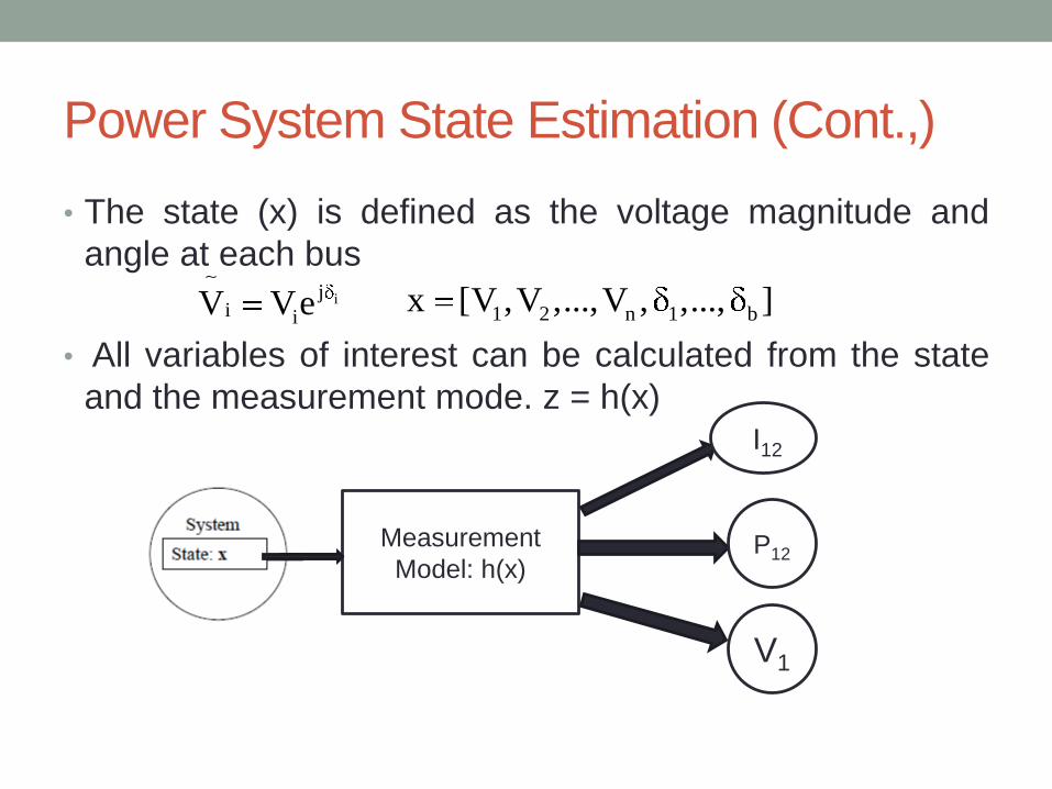
• The state (x) is defined as the voltage magnitude and
angle at each bus
• All variables of interest can be calculated from the state
and the measurement mode. z = h(x)
iji iV Ve
1 2 n 1 bx [V ,V ,...,V , ,..., ]
Measurement
Model: h(x)
I12
P12
V1

Power System State Estimation (Cont.,)
• We generally cannot directly observe the state
But we can infer it from measurements
The measurements are noisy (gross measurement
errors, communication channels outage)
Ideal
measurement:
H(x)
Noisy
Measurements
z=h(x)+e
Measurement: z

Consider a Simple DC Load Flow Example
Three-bus DC Load FlowThe only information we have about this system
is provided by three MW power flow meters

(Cont.,) Only two of these meter readings are required to calculate the bus
phase angles and all load and generation values fully
Now calculating the angles, considering third bus as swing bus we get
13M 5MW 0.05pu
32M 40MW 0.40pu
13 1 3 13
13
32 3 2 32
23
1f ( ) M 0.05pu
x
1f ( ) M 0.40pu
x
1
2
0.02rad
0.10rad

Case with all meters have small errors
If we use only the M13 and M32 readings,
as before, then the phase angles will be:
This results in the system flows as shown in
Figure . Note that the predicted flows match at
M13, and M32 but the flow on line 1-2 does not
match the reading of 62 MW from M12.
1
2
3
0.024rad
0.0925rad
0rad(still assumed to equal zero )
12
13
32
M 62MW 0.62pu
M 6MW 0.06pu
M 37MW 0.37pu

Power System State Estimation (Cont.,)
• The only thing we know about the power system comes tous from the measurements so we must use themeasurements to estimate system conditions.
• Measurements were used to calculate the angles atdifferent buses by which all unmeasured power flows,loads, and generations can be calculated.
• We call voltage angles as the state variables for the three-bus system since knowing them allows all other quantitiesto be calculated
• If we can use measurements to estimate the “states” ofthe power system, then we can go on to calculate anypower flows, generation, loads, and so forth that wedesire.

State Estimation: determining our best guess at the state
• We need to generate the best guess for the state giventhe noisy measurements we have available.
• This leads to the problem how to formulate a “best”estimate of the unknown parameters given the availablemeasurement.
• The traditional methods most commonly encounteredcriteria are
The Maximum likelihood criterion
The weighted least-squares criterion.
• Non traditional methods like
Evolutionary optimization techniques like GeneticAlgorithms, Differential Evolution Algorithms etc.,

Solution MethodologiesWeighted Least Square (WLS)method:
Minimizes the weighted sum of squares of the difference between
measured and calculated values .
In weighted least square method, the objective function „f‟ to be
minimized is given by
Iteratively Reweighted Least Square (IRLS)Weighted Least Absolute
Value (WLAV)method:
Minimizes the weighted sum of the absolute value of difference
between measured and calculated values.
The objective function to be minimized is given by
The weights get updated in every iteration.
m
2i2
i 1 i
1e
i
m| p |
i 1

(Cont.,)Least Absolute Value(LAV) method:
Minimizes the objective function which is the sum of absolutevalue of difference between measured and calculated values.
The objective function „g‟ to be minimized is given by g=
Subject to constraint zi= hi(x) + ei
Where, σ2 = variance of the measurement
W=weight of the measurement (reciprocal of variance of themeasurement)
ei = zi-hi(x), i=1, 2, 3 ….m.
h(x) = Measurement function, x = state variables and Z= MeasuredValue
m=number of measurements
mW
ii 1
| h (x)-z |i i

(Cont.,)
• The measurements are assumed to be in error: that is, the
value obtained from the measurement device is close to
the true value of the parameter being measured but differs
by an unknown error.
• If Zmeas be the value of a measurement as received from a
measurement device.
• If Ztrue be the true value of the quantity being measured.
• Finally, let η be the random measurement error.
Then mathematically it is expressed as
meas trueZ Z

(Cont.,)
•
2 21PDF( ) exp( / 2 )
2

20
Probability Distribution of Measurement Errors
3
f(x)
x
0
Gaussian
distibutionActual
distribution
Weighted least Squares-State Estimator
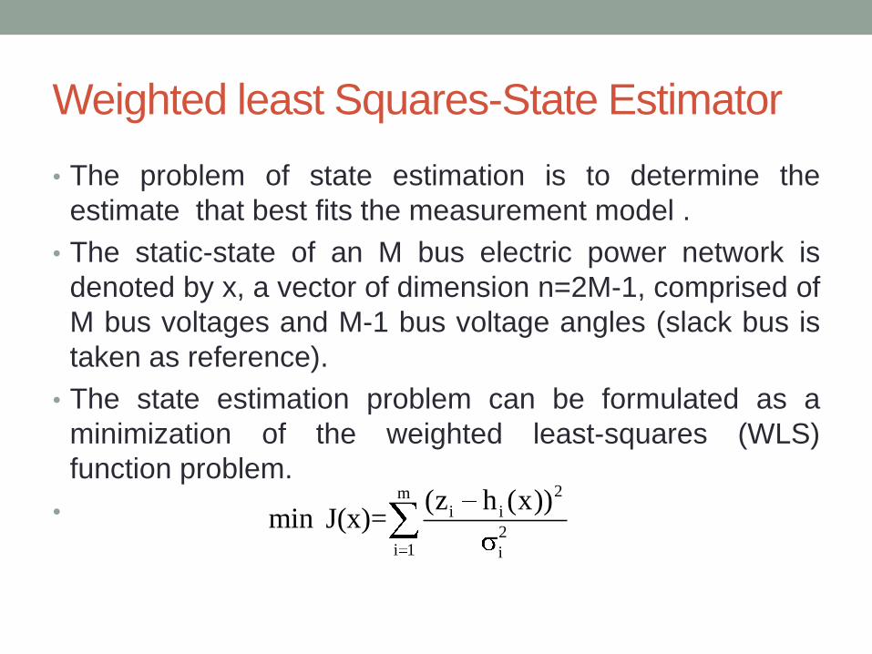
• The problem of state estimation is to determine the
estimate that best fits the measurement model .
• The static-state of an M bus electric power network is
denoted by x, a vector of dimension n=2M-1, comprised of
M bus voltages and M-1 bus voltage angles (slack bus is
taken as reference).
• The state estimation problem can be formulated as a
minimization of the weighted least-squares (WLS)
function problem.
•2m
i i
2i 1 i
(z h (x))min J(x)=

(Cont.,)
• This represents the summation of the squares of themeasurement residuals weighted by their respectivemeasurement error covariance.
• where, z is measurement vector.
h(x) is measurement matrix.
m is number of measurements.
σ2 is the variance of measurement.
x is a vector of unknown variables to be estimated.
• The problem defined is solved as an unconstrainedminimization problem.
• Efficient solution of unconstrained minimization problemsrelies heavily on Newton‟s method.

(Cont.,)
• The type of Newton‟s method of most interest here is the
Gauss-Newton method.
• In this method the nonlinear vector function is linearized
using Taylor series expansion
• where, the Jacobian matrix H(x) is defined as:
• Then the linearized least-squares objective function is
given by
h(x x) h(x) H(x) x
h(x)H(x)
x
T 11J( x) (z h(x) H(x) x) R (z h(x) H(x) x)
2

(Cont.,)
• where, R is a weighting matrix whose diagonal elements
are often chosen as measurement error variance, i.e.,
• where, e=z-h(x) is the residual vector.
2
1
2
m
R
T 11J( x) (e(x) H(x) x) R (e(x) H(x) x)
2

(Cont.,)
•
T 1J( x)H R (e H x) 0
x
T 1 T 1H R H x H R e
T 1G x H R e

Weighted Least Squares-Example•
est
1est
est
2
x

(Cont.,)
• To derive the [H] matrix, we need to write the measurements
as a function of the state variables . These functions
are written in per unit as1 2and
12 12 1 2 1 2
13 13 1 3 1
32 32 3 2 2
1M f ( ) 5 5
0.2
1M f ( ) 2.5
0.4
1M f ( ) 4
0.25

(Cont.,)
•
5 5
[H] 2.5 0
0 4
2 2
M12 M12
2 2
M13 M13
2 2
M32 M32
0.0001
R 0.0001
0.0001

(Cont.,)
•
11
est
1
est
2
1
0.0001 5 55 2.5 0
0.0001 2.5 05 0 4
0.0001 0 4
0.0001 0.625 2.5 0
0.0001 0.065 0 4
0.0001 0.3
- -
- -7

(Cont.,)
• We get
• From the estimated phase angles, we can calculate the
power flowing in each transmission line and the net
generation or load at each bus.
est
1
est
2
0.028571
0.094286
2 2 2
1 2 1 21 2
(0.62 (5 5 )) (0.06 (2.5 )) (0.37 (4 ))J( , )
0.0001 0.0001 0.0001
2.14

Solution of the weighted least square example

Bad Data Processing
• One of the essential functions of a state estimator is todetect measurement errors, and to identify and eliminatethem if possible.
• Measurements may contain errors due to
Random errors usually exist in measurements due tothe finite accuracy of the meters
Telecommunication medium.
• Bad data may appear in several different ways dependingupon the type, location and number of measurements thatare in error. They can be broadly classified as:
Single bad data: Only one of the measurements inthe entire system will have a large error
• Multiple bad data: More than one measurement will be inerror

(Cont.,)• Critical measurement: A critical measurement is the one whose
elimination from the measurement set will result in an unobservablesystem. The measurement residual of a critical measurement willalways be zero.
• A system is said to be observable if all the state variables can becalculated with available set of measurements.
• Redundant measurement: A redundant measurement is ameasurement which is not critical. Only redundant measurementsmay have nonzero measurement residuals.
• Critical pair: Two redundant measurements whose simultaneousremoval from the measurement set will make the systemunobservable.

(Cont.,)• When using the WLS estimation method, detection and
identification of bad data are done only after the estimation
process by processing the measurement residuals.
• The condition of optimality is that the gradient of J(x) vanishes
at the optimal solution x, i.e.,
• An estimate z of the measurement vector z is given by
• The vector of residuals is defined as e = z - Hx; an estimate of
e is given by
( h( ) 'J x z x) W z h(x)
1GX H WZ 0 1 1 X G H WZ
Z HX
e z h(x)

Bad Data Detection and Identification
• Detection refers to the determination of whether or not themeasurement set contains any bad data.
• Identification is the procedure of finding out which specificmeasurements actually contain bad data.
• Detection and identification of bad data depends on theconfiguration of the overall measurement set in a givenpower system.
• Bad data can be detected if removal of the correspondingmeasurement does not render the system unobservable.
• A single measurement containing bad data can beidentified if and only if:
it is not critical and
it does not belong to a critical pair

Bad Data Detection
•
N2
i
i 1
Y X
2
kY

Chi-square probability density function

Chi-squares distribution table
(Cont.,)
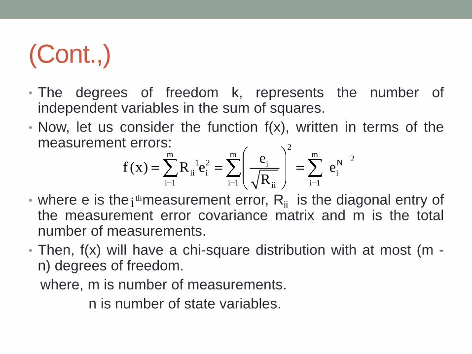
• The degrees of freedom k, represents the number ofindependent variables in the sum of squares.
• Now, let us consider the function f(x), written in terms of themeasurement errors:
• where e is the measurement error, Rii is the diagonal entry ofthe measurement error covariance matrix and m is the totalnumber of measurements.
• Then, f(x) will have a chi-square distribution with at most (m -n) degrees of freedom.
where, m is number of measurements.
n is number of state variables.
thi
2m m m
21 2 Ni
ii i i
i 1 i 1 i 1ii
ef (x) R e e
R

Steps to detection of bad data
•
m2 2
i i
j 1
f e / .
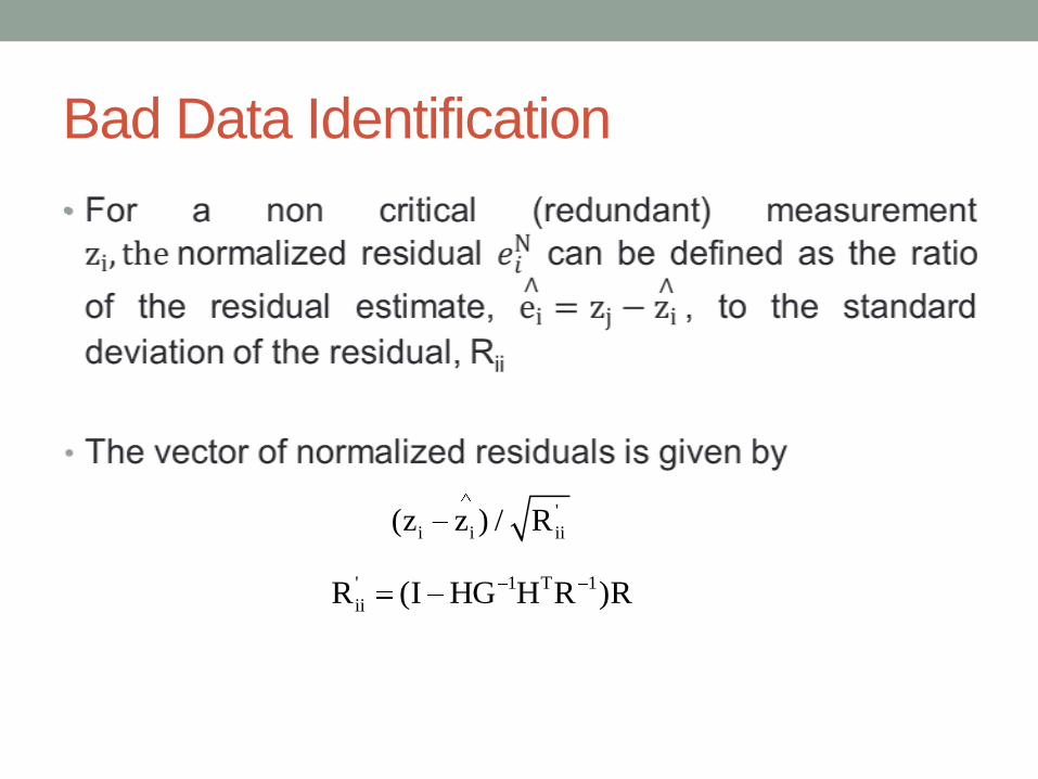
Bad Data Identification
•
'
i i ii(z z ) / R
' 1 T 1
iiR (I HG H R )R

Steps to Bad Data Identification
•
N i
i'
ii
ee
R i=1,2,...m
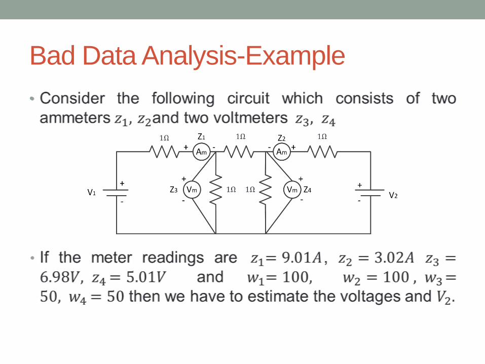
Bad Data Analysis-Example
•

Cont.,
• Measurement equations characterizing the meter
readings are found by adding errors terms to the system
model. We obtain
1 1 2 1
2 1 2 2
3 1 2 3
4 1 2 4
5 1z x x e
8 8
1 8z x x e
8 8
3 1z x x e
8 8
1 3z x x e
8 8

(Cont.,)
• Forming the H matrix we get
0.625 0.125
0.125 0.625H
0.375 0.125
0.125 0.375
100 0 0 0
0 100 0 0W
0 0 50 0
0 0 0 509.01
3.02z
6.98
5.01

(Cont.,)
• Solving for state estimates i.e.,
• We get
11 T
2
VG H Wz
V
1
2
V 16.0072V
8.0261VV
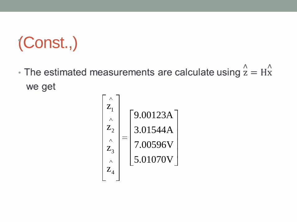
(Const.,)•
1
2
3
4
z9.00123A
z 3.01544A
7.00596Vz
5.01070Vz

(Cont.,)
•
1
2
3
4
e9.01 9.00123 0.00877A
e 3.02 3.01544 0.00456A
6.98 7.00596 0.02596Ve
5.01 5.01070 0.00070Ve

(Cont.,)
•
42 2 2 2 2 2
i i
j 1
f e / 100(0.00877) 100(0.00456) 50(0.02596) 50(0.00070)
0.043507

(Cont.,)
•
T T
1 2 3 4[z z z z ] [9.01A 3.02A 6.98V 4.40V]
T T
1 2 3 4[e e e e ] [9.01A 3.02A 6.98V 4.40V]
42 2 2 2 2 2
i i
j 1
f e / 100(0.06228) 100(0.15439) 50(0.05965) 50(0.49298)
15.1009

(Cont.,)
•
' 1 T 1
iiR (I HG H R )R
iN
i'
ii
e
eR
i=1,2,...m
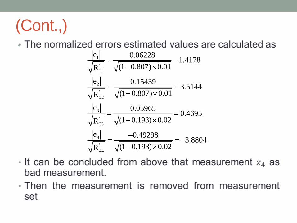
(Cont.,)•
1
'
11
2
'
22
3
'
33
4
'
44
e 0.062281.4178
(1 0.807) 0.01R
e 0.154393.5144
(1 0.807) 0.01R
e 0.059650.4695
(1 0.193) 0.02R
e 0.492983.8804
(1 0.193) 0.02R

Conclusion
• Real time monitoring and control of power systems isextremely important for an efficient and reliable operationof a power system.
• Sate estimation forms the backbone for the real timemonitoring and control functions.
• In this environment, a real-time model is extracted atintervals from snapshots of real-time measurements.
• Estimate the nodal voltage magnitudes and phase anglestogether with the parameters of the lines.
• State estimation results can be improved by usingaccurate measurements like phasor measurement units.
• Traditional state estimation and bad data processing isreviewed.
References• F. C. Schweppe and J. Wildes, “Power system static state estimation, part I: exactmodel,” IEEE Trans. Power Apparatus and Systems, vol. PAS-89, pp. 120-125,Jan. 1970.
• R. E. Tinney W. F. Tinney, and J. Peschon, “State estimation in power systems,part i: theory and feasibility,” IEEE Trans. Power Apparatus and Systems, vol.PAS-89, pp. 345-352, Mar. 1970.
• F. C. Schweppe and D. B. Rom, “Power system static-state estimation, part ii:approximate model,” IEEE Trans. Power Apparatus and Systems, vol. PAS-89,pp.125-130, Jan. 1970.
• F. F. Wu, “Power System State Estimation,” International Journal of ElectricalPower and Energy Systems, vol. 12, Issue. 2, pp. 80-87, Apr. 1990.
• Ali Abur and Antonio Gomez Exposito. (2004, April). Power System StateEstimation Theory and Implementation (1st ed.) [Online]. Available:http://www.books.google.com.
• Allen J wood and Bruce F Wollenberg. (1996, February 6). Power Generation,Operation, and Control (2nd ed.) [Online]. Available:http://www.books.google.com.


