UNCERTAINTY AND STATE ESTIMATION OF POWER SYSTEMS A Thesis submitted to The University of Manchester for the degree of Doctor of Philosophy In the Faculty of Engineering and Physical Sciences 2012 by Gustavo Adolfo Valverde Mora School of Electrical and Electronic Engineering
Transcript
UNCERTAINTY AND STATE ESTIMATION OF POWER SYSTEMS
A Thesis submitted to The University of Manchester for the degree of
Doctor of Philosophy
In the Faculty of Engineering and Physical Sciences
2012
by
Gustavo Adolfo Valverde Mora
School of Electrical and Electronic Engineering
Preface
1
List of Content
List of Content ............................................................................................................................ 1 List of Figures ............................................................................................................................. 4 List of Tables .............................................................................................................................. 7 Abstract ....................................................................................................................................... 8 Declaration .................................................................................................................................. 9 Copyright Statement ................................................................................................................ 10 Acknowledgements .................................................................................................................. 12 Chapter 1 Introduction ...................................................................................................... 13
1.1 Research Background ................................................................................................ 14 1.1.1 Probabilistic Load Flows ................................................................................... 14 1.1.2 State Estimation ................................................................................................. 16 1.1.3 Synchronised Measurements ............................................................................. 17 1.1.4 Hybrid State Estimators ..................................................................................... 18
1.2 Objectives .................................................................................................................. 19 1.3 Thesis Structure ......................................................................................................... 19 1.4 Contribution of this Research .................................................................................... 22
Chapter 2 Classical State Estimation in Power Systems ...................................................... 24 2.1 WLS Formulation ...................................................................................................... 26
2.3 Redundancy Analysis ................................................................................................. 35 2.4 Bad Data Processing .................................................................................................. 36
2.4.1 Chi square Distribution Test .............................................................................. 37 2.4.2 Measurement Residuals ..................................................................................... 38 2.4.3 Normalized Residual Test .................................................................................. 40
Chapter 3 Estimation of Probabilistic Load Flows: Theory and Modelling ...................... 42 3.1 Gaussian Mixture Distribution ................................................................................... 43 3.2 Reduction of Gaussian Mixtures ................................................................................ 48
3.2.1 Fine Tuning of GMM Reductions ...................................................................... 55 3.3 Probabilistic Load Flows ........................................................................................... 58
3.3.1 PLF using Monte Carlo Simulations .................................................................. 59 3.3.1.1 Generation of Samples from Correlated Variables ........................................ 59
4.1.1 14-bus IEEE Test System .................................................................................. 69 4.1.1.1 Case 1 in 14-bus system ................................................................................. 70 4.1.1.2 Case 2 in 14-bus system ................................................................................. 74
Preface
2
4.1.2 57-bus IEEE Test System Simulation ................................................................ 78 4.2 Radial Networks......................................................................................................... 87
4.2.1 69-bus IEEE Test System Simulations .............................................................. 88 4.2.1.1 Case 1: Probabilistic Load Flows .................................................................. 89 4.2.1.2 Case 2: State Estimation ................................................................................ 93 4.2.1.3 Selection of GMM for Reduction .................................................................. 97
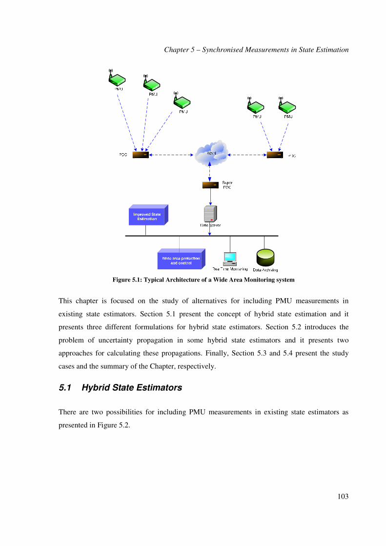
Chapter 5 Synchronised Measurements in State Estimation ............................................ 102 5.1 Hybrid State Estimators ........................................................................................... 103
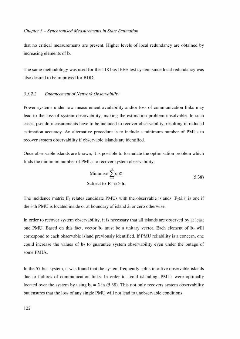
5.3 Study Cases .............................................................................................................. 119 5.3.1 SE Performance Index ..................................................................................... 119 5.3.2 Placement of PMUs and Conventional Measurements .................................... 120
Chapter 7 Dynamic State Estimation .......................................................................... 149 7.1 Dynamic State Estimators ........................................................................................ 150
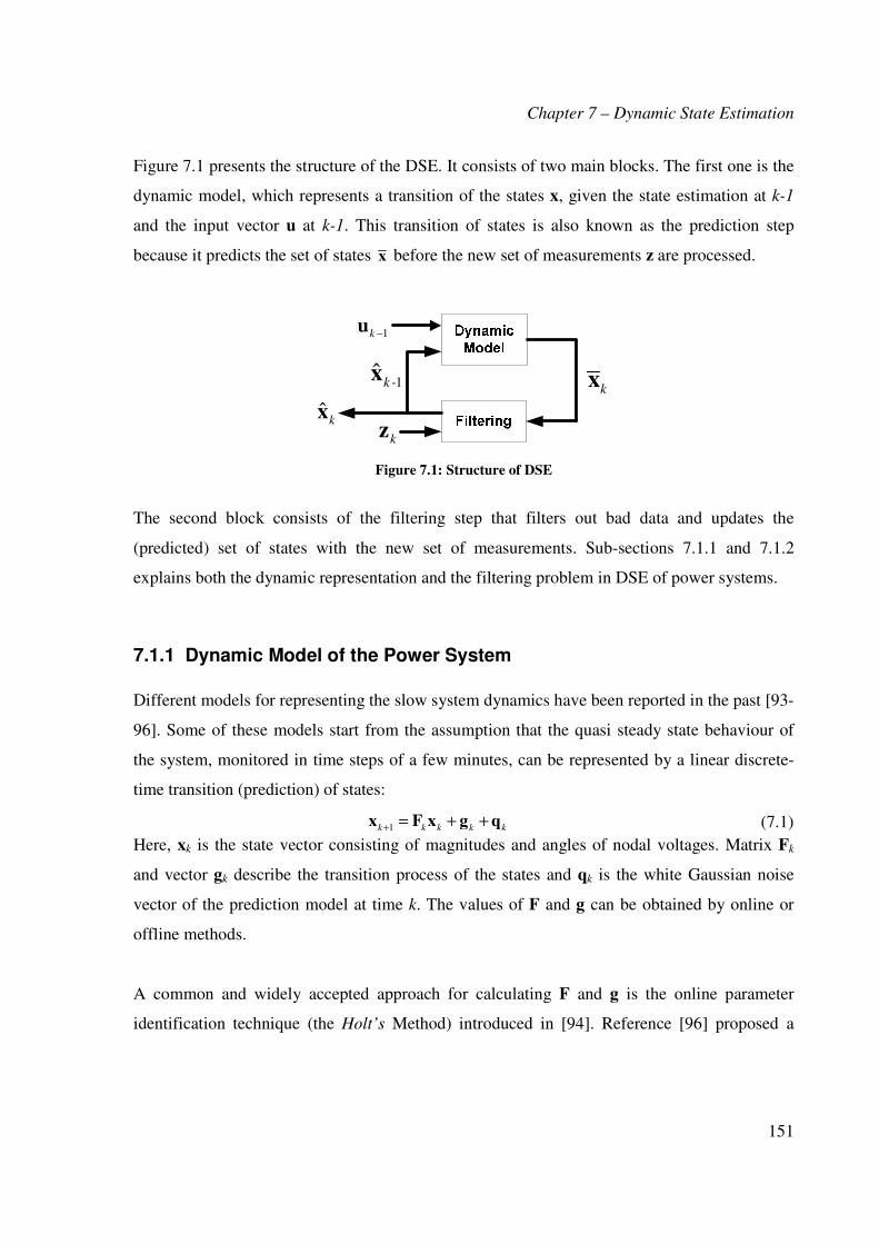
7.1.1 Dynamic Model of the Power System ............................................................. 151 7.1.2 Filtering Problem ............................................................................................. 152
7.2 Kalman Filters .......................................................................................................... 152 7.2.1 The Extended Kalman Filter ............................................................................ 154 7.2.2 The Unscented Kalman Filter .......................................................................... 155
7.2.2.1 Sigma Points Calculation ............................................................................. 156 7.2.2.2 Kalman Filter State Prediction ..................................................................... 157 7.2.2.3 Kalman Filter State Correction .................................................................... 157
7.3 Power System State Estimation using the UKF ....................................................... 159
Preface
3
7.3.1 Dynamic Model of the System ........................................................................ 159 7.3.2 State Prediction and Correction ....................................................................... 160 7.3.3 Detection of Anomalies ................................................................................... 161
7.4 Study Cases .............................................................................................................. 163 7.4.1 Performance Indices ......................................................................................... 164 7.4.2 Simulation Results ........................................................................................... 164
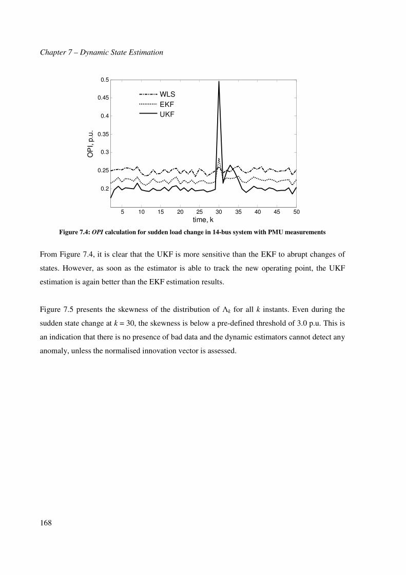
7.4.2.1 Normal Operation Case in 14-bus Test System ........................................... 165 7.4.2.2 Sudden Load Changes in 14-bus Test System ............................................. 167 7.4.2.3 Presence of Large Bad Data in 57-bus Test System .................................... 170
10.1 Appendix A .............................................................................................................. 192 10.1.1 A.1: Solution of WLS Formulation ................................................................. 192 10.1.2 A.2: Solution of constraint WLS Formulation ................................................. 193
10.2 Appendix B .............................................................................................................. 195 10.2.1 B.1: LU Decomposition ................................................................................... 195
10.3 Appendix C .............................................................................................................. 197 10.3.1 C.1: Solution of sub-vector hj(·) ....................................................................... 197 10.3.2 C.2: Solution of matrix P(·) ............................................................................. 198
10.4 Appendix D .............................................................................................................. 199 10.4.1 D.1: Power Flow Calculation in Radial Networks ........................................... 199
10.5 Appendix E .............................................................................................................. 201 10.5.1 E.1: The Kalman Filter .................................................................................... 201
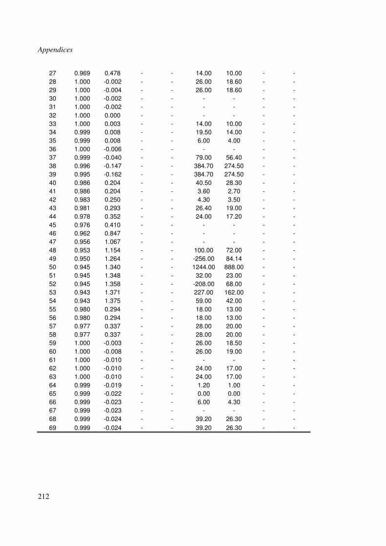
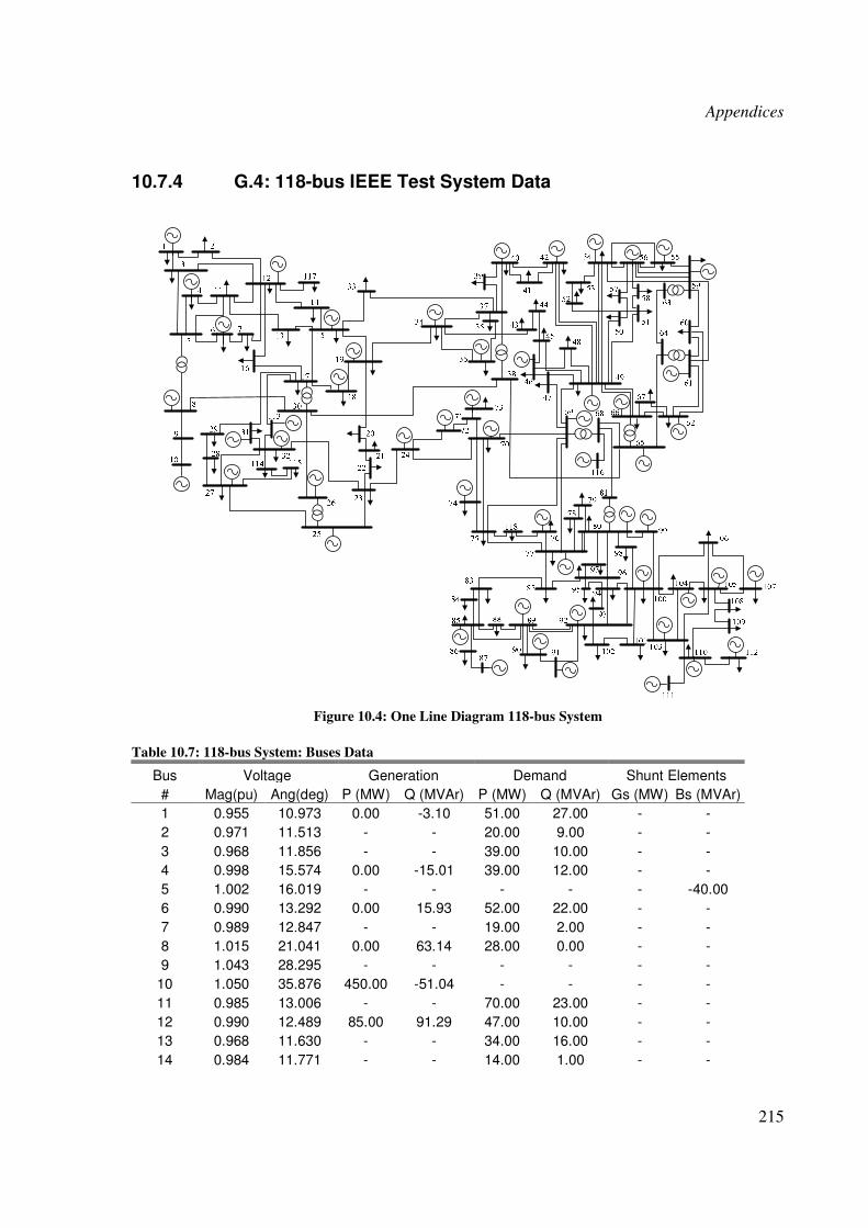
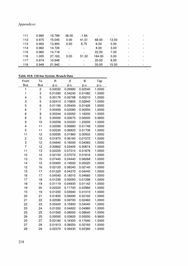
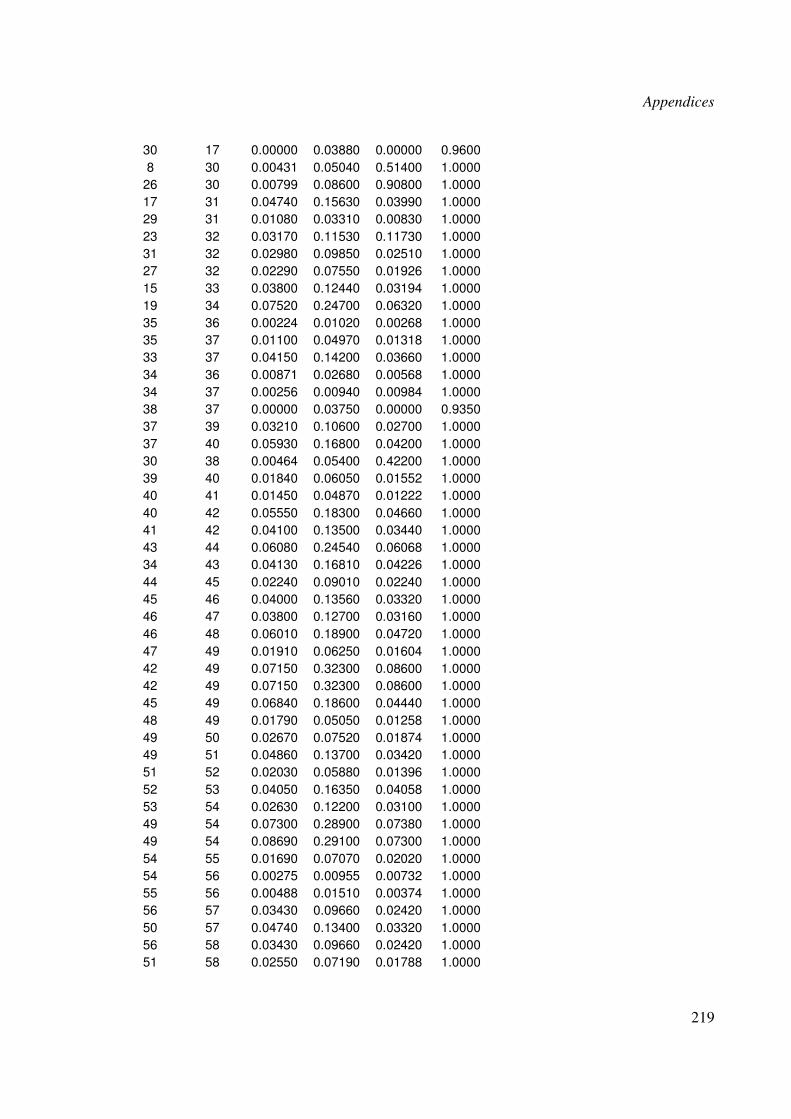
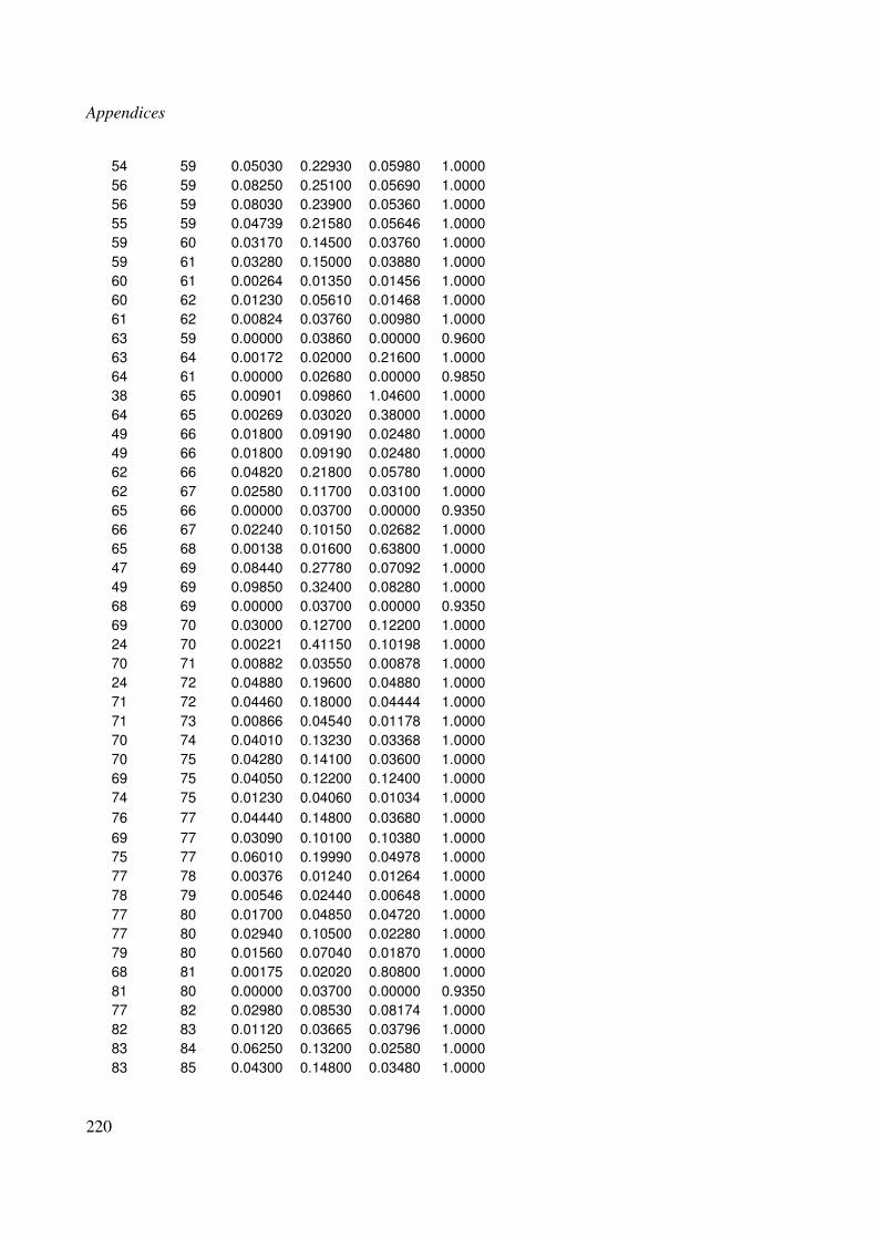
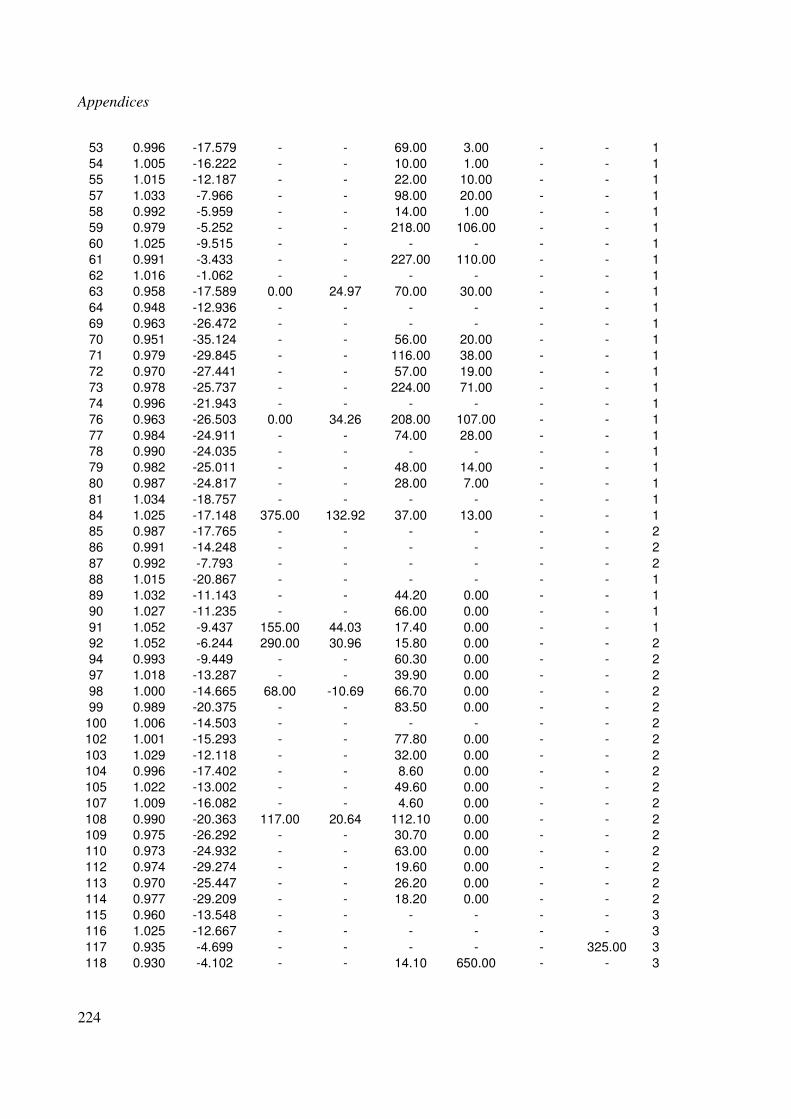
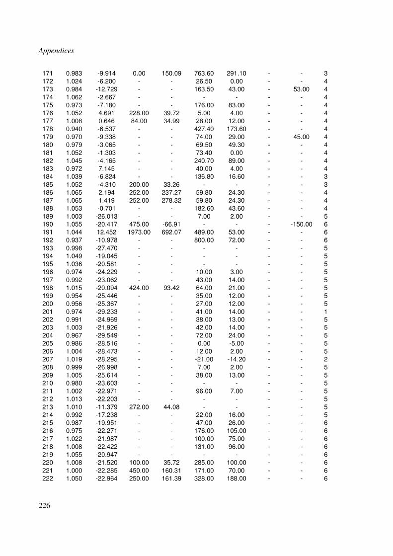
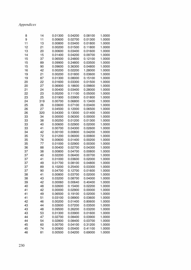
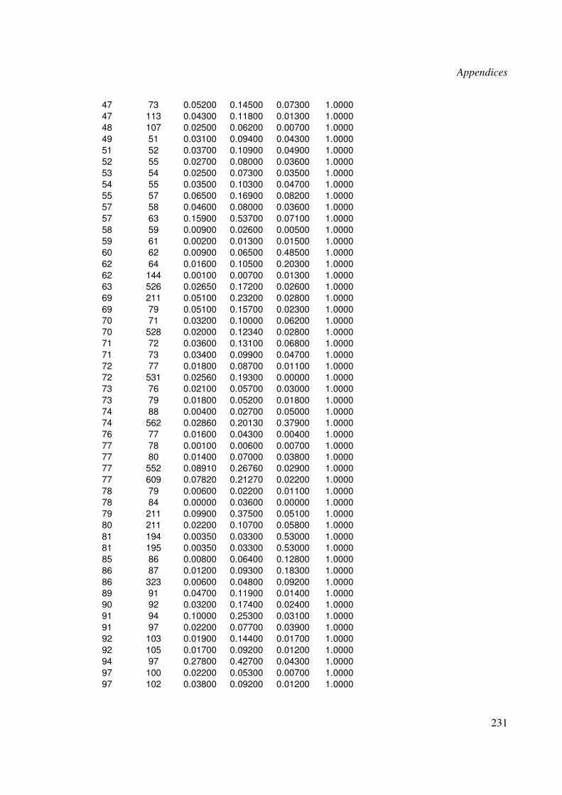
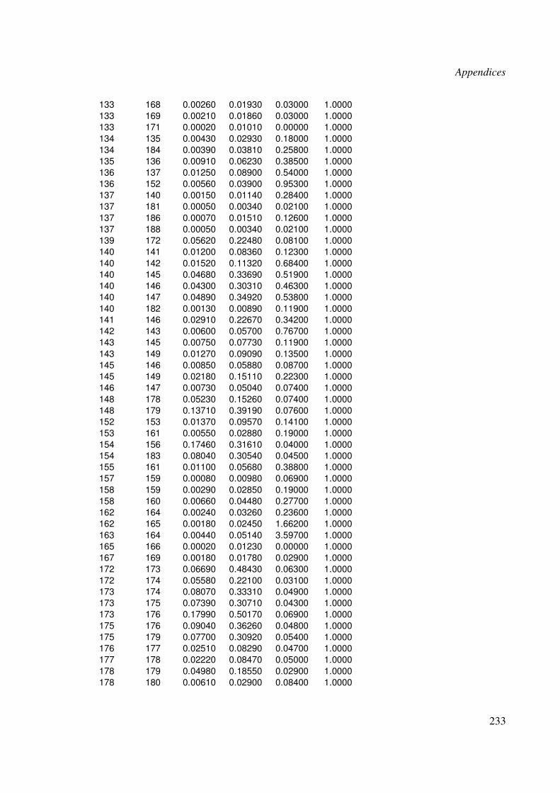
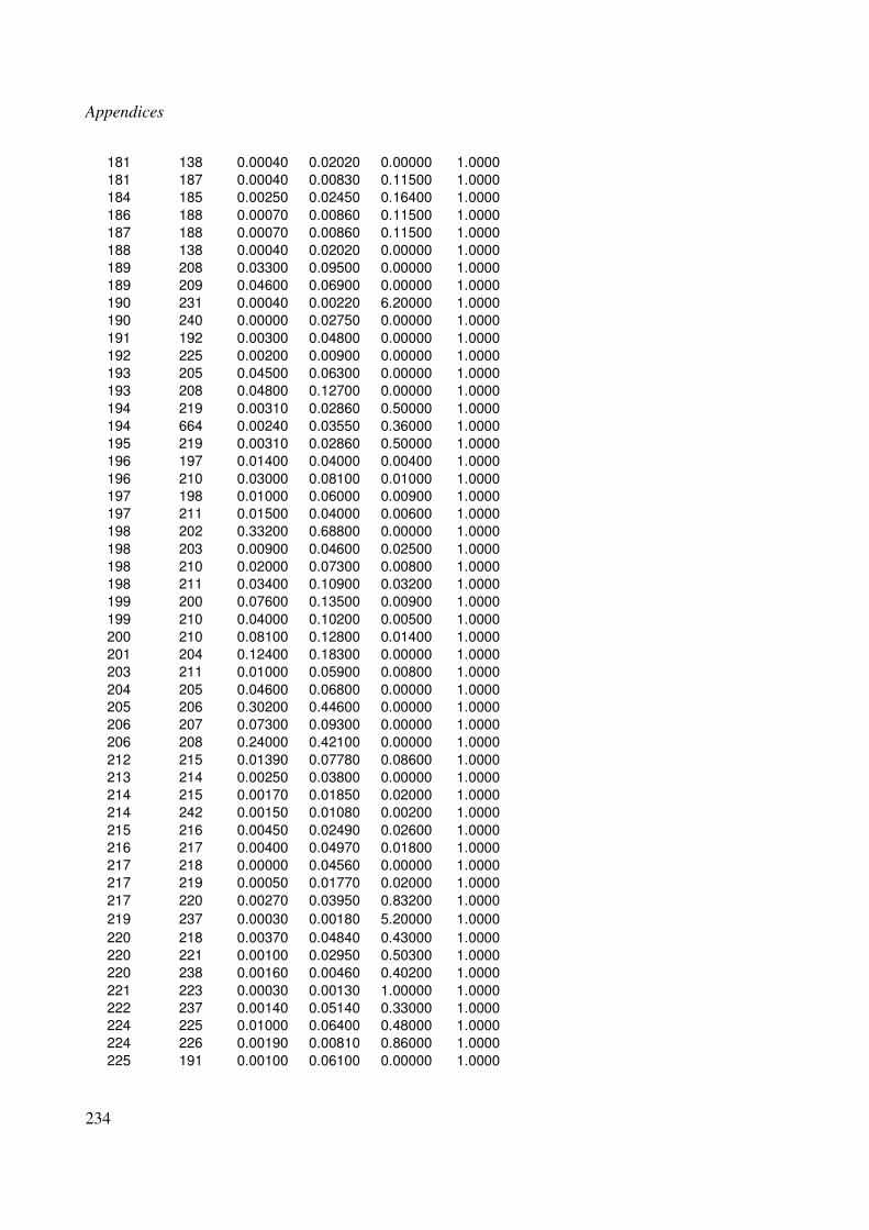
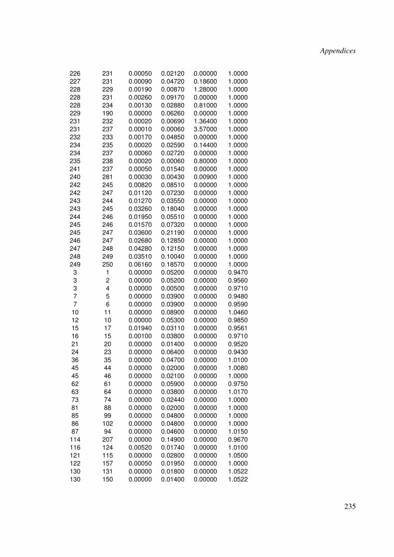
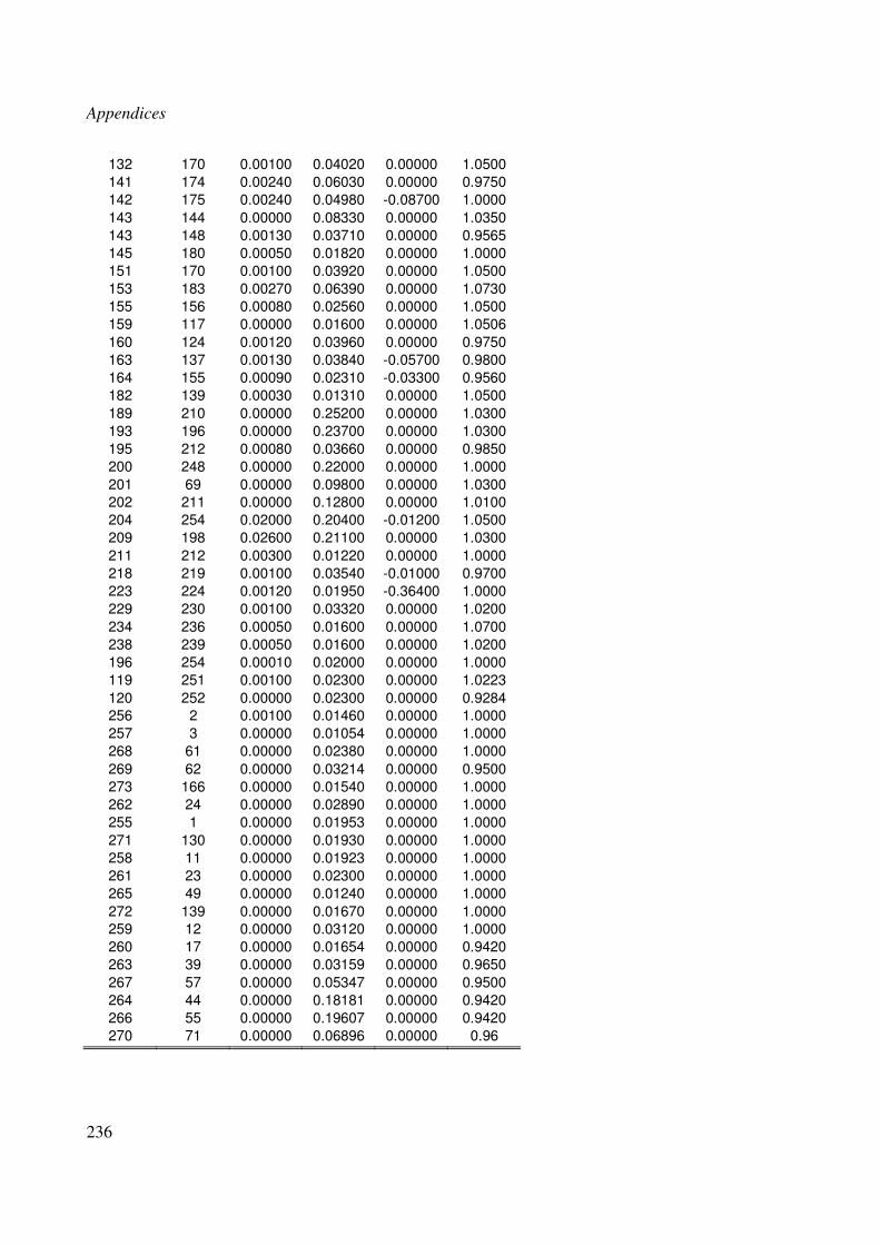
10.7 Appendix G .............................................................................................................. 205 10.7.1 G.1: 14-bus IEEE Test System Data ................................................................ 205 10.7.2 G.2: 57-bus IEEE Test System Data ................................................................ 207 10.7.3 G.3: 69-bus IEEE Test System Data ................................................................ 211 10.7.4 G.4: 118-bus IEEE Test System Data .............................................................. 215 10.7.5 G.5: 300-bus IEEE Test System Data .............................................................. 223
10.8 Appendix H .............................................................................................................. 237 10.8.1 H.1 Published Journal Papers .......................................................................... 237 10.8.2 H.2 Submitted Journal Papers .......................................................................... 237 10.8.3 H.3 Published Conference Papers .................................................................... 237
Final count: 54 152 words.
Preface
4
List of Figures Figure 1.1: PhD Thesis Structure ............................................................................................... 22
Figure 2.1: 14-bus system with conventional set of measurements ........................................... 24
Figure 2.2: Building block of a state estimator .......................................................................... 25
Figure 2.3: Pi-model of network branch including tap modelling ............................................. 28
Figure 2.4: Chi Square PDF for 20 degrees of freedom ............................................................ 37
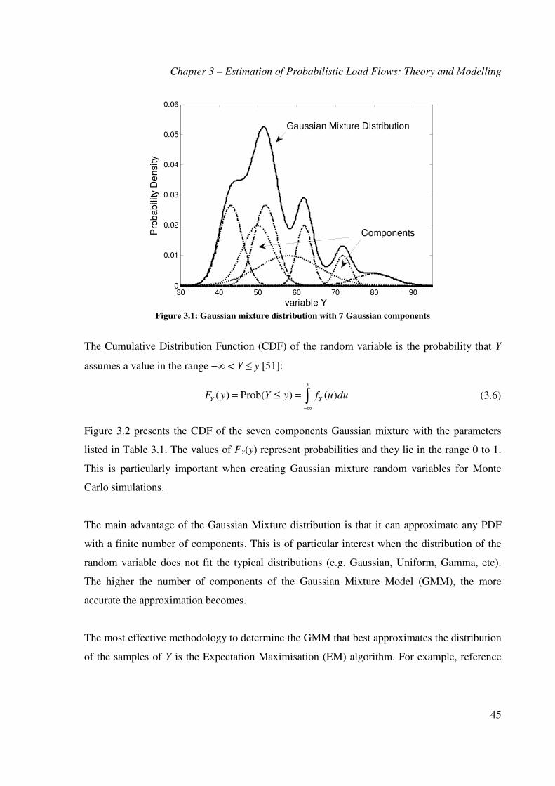
Figure 3.1: Gaussian mixture distribution with 7 Gaussian components .................................. 45
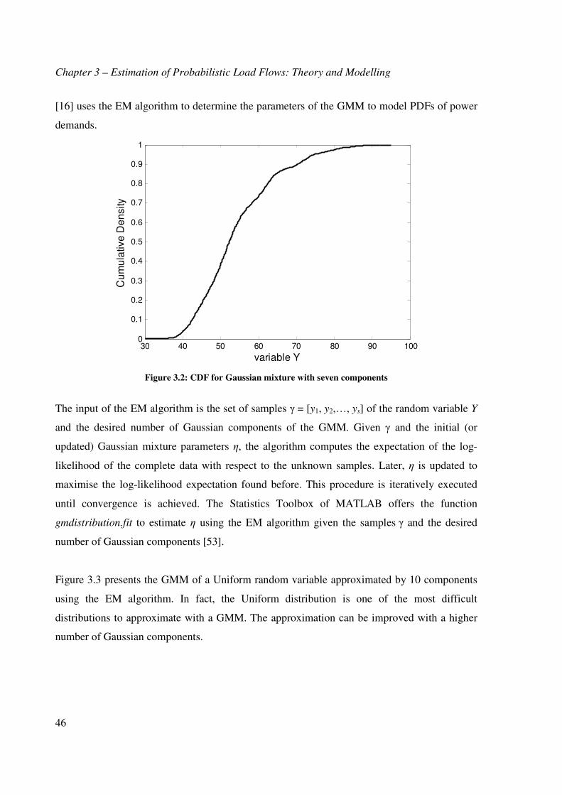
Figure 3.2: CDF for Gaussian mixture with seven components ................................................ 46
Figure 3.3: Uniform distributed random variable modelled by GMM ...................................... 47
Figure 3.4: Gamma distributed random variable modelled by GMM ....................................... 47
Figure 3.5: GMM reduction using five components .................................................................. 52
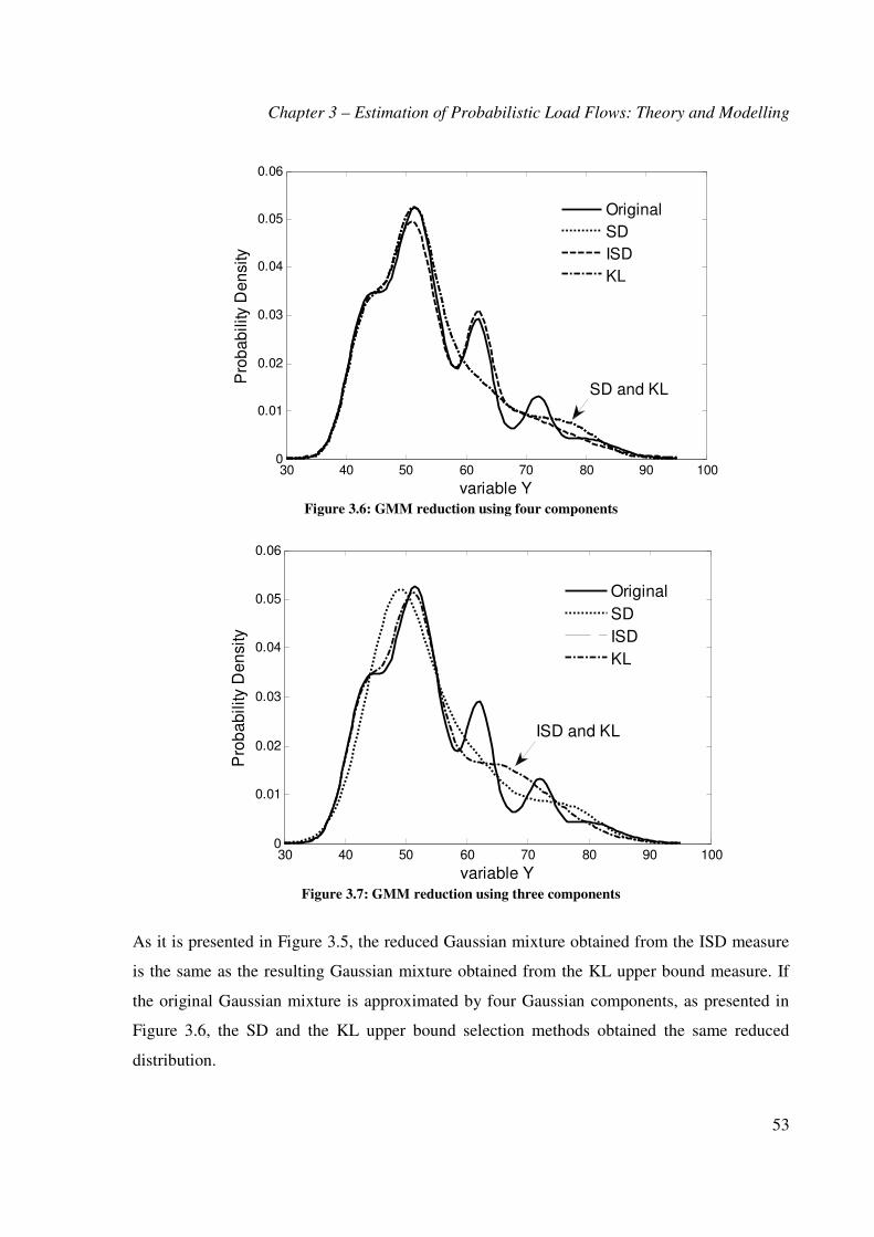
Figure 3.6: GMM reduction using four components ................................................................. 53
Figure 3.7: GMM reduction using three components ................................................................ 53
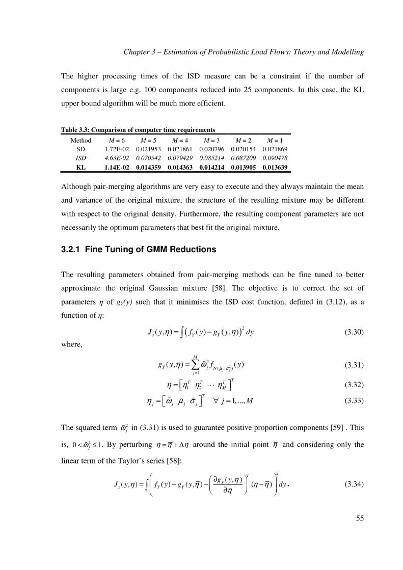
Figure 3.8: Original GMM reduced to four components using the optimal based method ....... 57
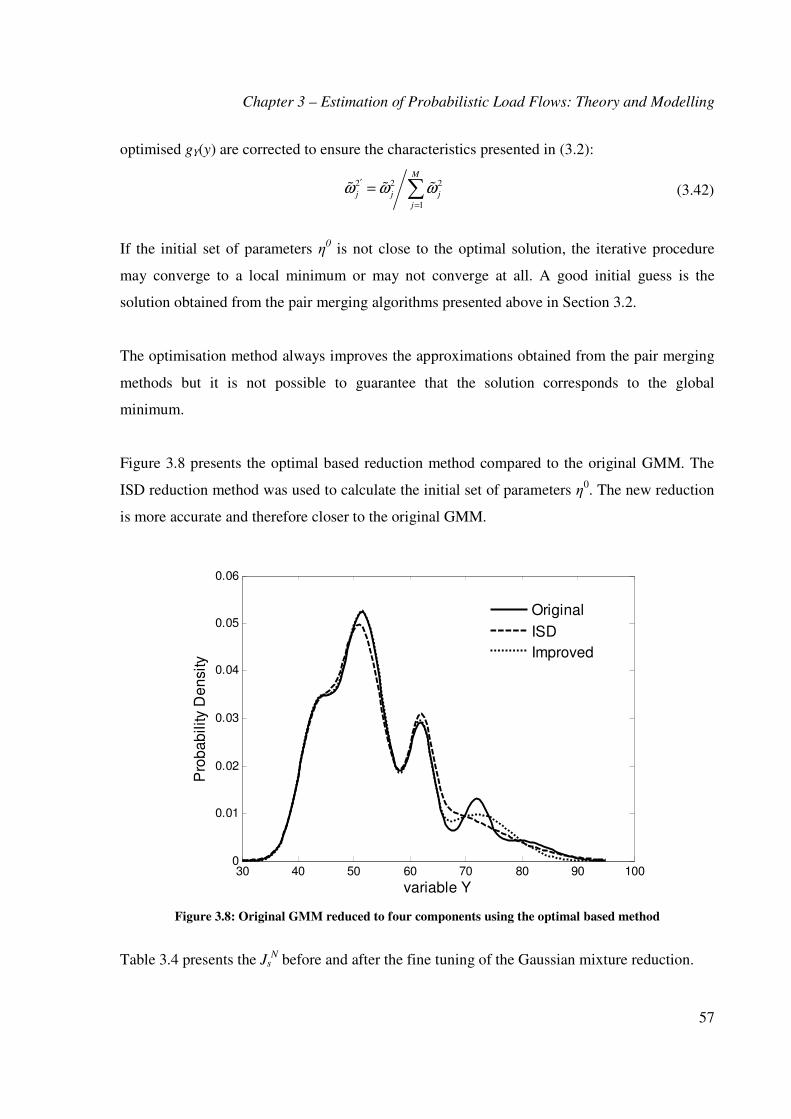
Figure 3.9: PLF problem with non-Gaussian PDFs ................................................................... 59
Figure 3.10: Scatter plot of resulting samples ........................................................................... 63
Figure 3.11: Histogram of resulting samples ............................................................................. 63
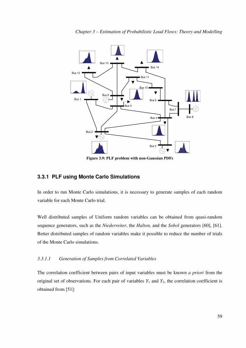
Figure 3.12: Diagram of probabilistic load flows using MCS ................................................... 64
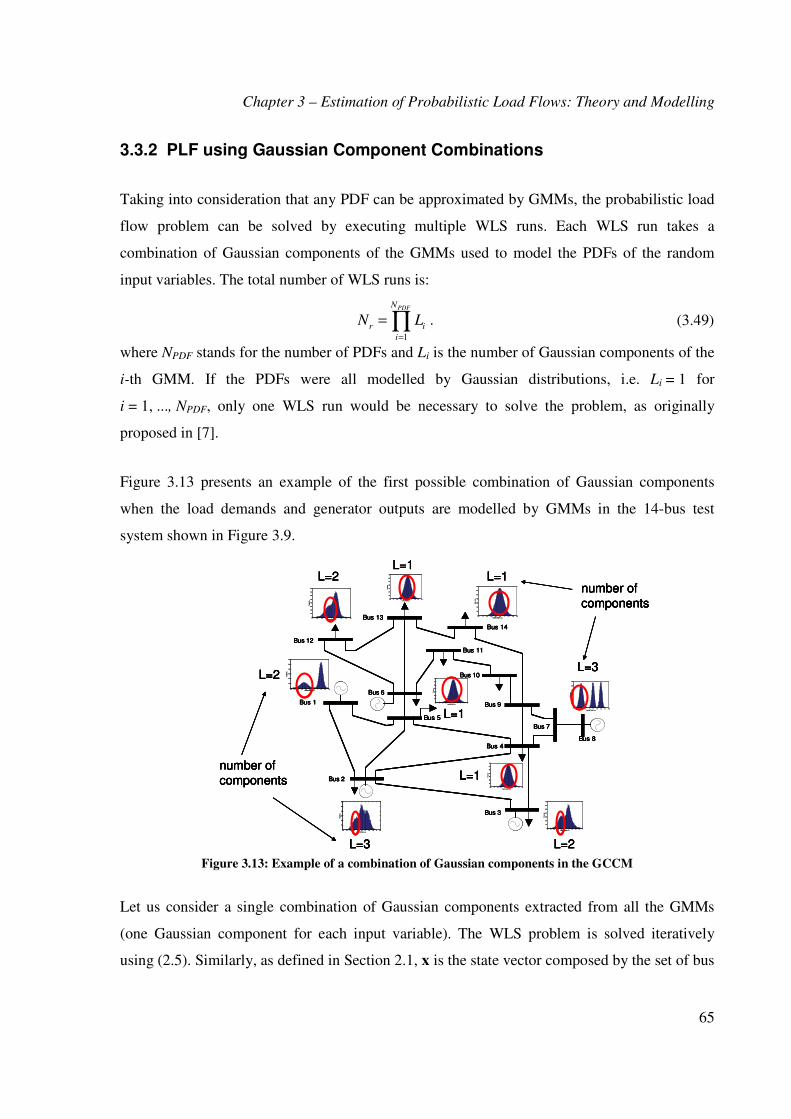
Figure 3.13: Example of a combination of Gaussian components in the GCCM...................... 65
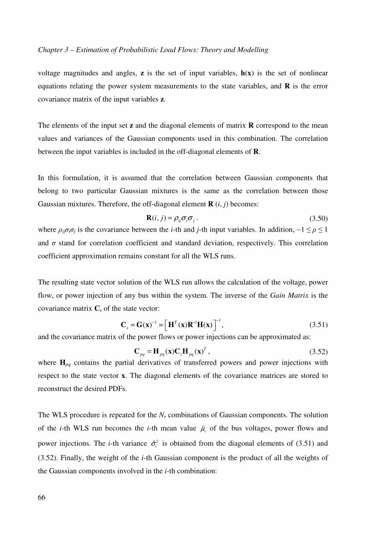
Figure 4.1: PDF of active power flow from Bus 2 to Bus 3 (case 1). ........................................ 72
Figure 4.2: PDF of reactive power flow from Bus 2 to Bus 3 (case 1). .................................... 72
Figure 4.3: PDF of active power flow from Bus 9 to Bus 14 (case 1). ...................................... 73
Figure 4.4: PDF of reactive power flow from Bus 9 to Bus 14 (case 1). .................................. 73
Figure 4.5: PDF of voltage magnitude and angle at Bus 13 (case 1)......................................... 74
Figure 4.6: PDF of active power flow from Bus 9 to Bus 14 (case 2). ...................................... 75
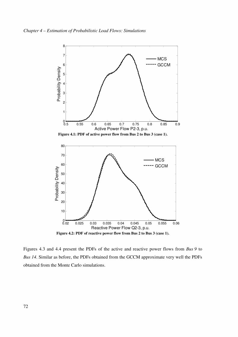
Figure 4.7: PDF of reactive power flow from Bus 9 to Bus 14 (case 2). .................................. 76
Figure 4.8: PDF of active power flow from Bus 13 to Bus 14 (case 2). .................................... 76
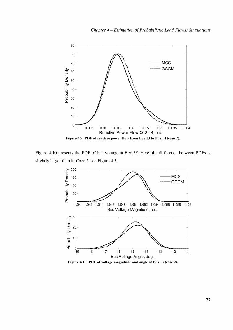
Figure 4.9: PDF of reactive power flow from Bus 13 to Bus 14 (case 2). ................................ 77
Figure 4.10: PDF of voltage magnitude and angle at Bus 13 (case 2)....................................... 77
Figure 4.11: PDF of P3-4 with reduced Gaussian components. ................................................ 80
Figure 4.12: PDF of Q3-4 with reduced Gaussian components. ............................................... 80
Figure 4.13: PDF of P2-3 with reduced Gaussian components. ................................................ 81
Figure 4.14: PDF of Q2-3 with reduced Gaussian components. ............................................... 81
Figure 4.15: PDF of P22-38 with reduced Gaussian components. ............................................ 82
Figure 4.16: PDF of Q22-38 with reduced Gaussian components. ........................................... 82
Figure 4.17: PDF of P21-20 with reduced Gaussian components. ............................................ 83
Figure 4.18: PDF of Q21-20 with reduced Gaussian components. ........................................... 83
Figure 4.19: PDF of P36-37 with reduced Gaussian components. ............................................ 84
Figure 4.20: PDF of Q36-37 with reduced Gaussian components. ........................................... 84
Figure 4.21: PDF of P38-49 with reduced Gaussian components. ............................................ 85
Figure 4.22: PDF of Q38-49 with reduced Gaussian components. ........................................... 85
Figure 4.23: PDF of voltage magnitude and angle at Bus 22 with reduced Gaussian components. ............................................................................................................................... 86
Preface
5
Figure 4.24: PDF of voltage magnitude and angle at Bus 36 with reduced Gaussian components. ............................................................................................................................... 86
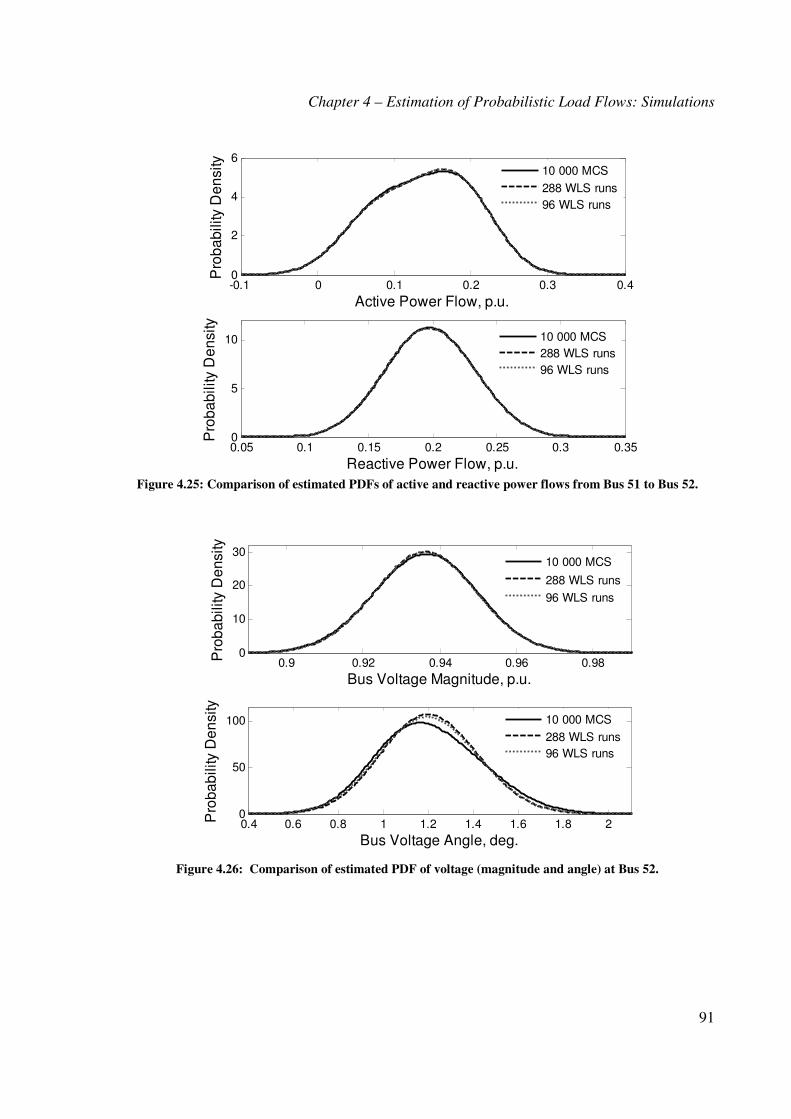
Figure 4.25: Comparison of estimated PDFs of active and reactive power flows from Bus 51 to Bus 52. ....................................................................................................................................... 91
Figure 4.26: Comparison of estimated PDF of voltage (magnitude and angle) at Bus 52. ...... 91
Figure 4.27: Comparison of estimated PDF of active and reactive power flows from Bus 20 to Bus 21. ....................................................................................................................................... 92
Figure 4.28: Comparison of estimated PDF of voltage (magnitude and angle) at Bus 21. ....... 92
Figure 4.29: Influence of correlation in estimated voltages on (a) Bus 27 and (b) Bus 56. ..... 93
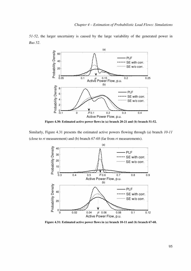
Figure 4.30: Estimated active power flows in (a) branch 20-21 and (b) branch 51-52. ............ 95
Figure 4.31: Estimated active power flows in (a) branch 10-11 and (b) branch 67-68. ............ 95
Figure 4.32: Estimated Voltage Magnitude at (a) Bus 21 and (b) Bus 52. ................................ 96
Figure 4.33: Estimated Voltage Magnitude at (a) Bus 11 and (b) Bus 68. ................................ 96
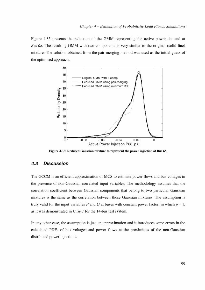
Figure 4.34: JsN for reduced Gaussian mixtures using (a) the pair merging method and (b) the
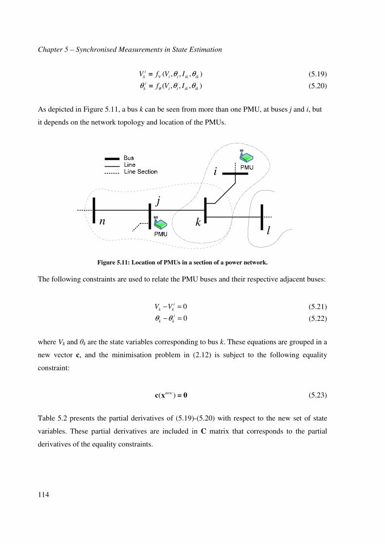
Figure 5.11: Location of PMUs in a section of a power network. ........................................... 114
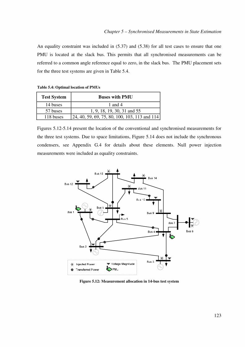
Figure 5.12: Measurement allocation in 14-bus test system .................................................... 123
Figure 5.13: Measurement allocation in 57-bus test system .................................................... 124
Figure 5.14: Measurement allocation in 118-bus test system .................................................. 124
Figure 5.15: Voltage angle estimation errors for the IEEE 14 bus test system. ...................... 126
Figure 5.16: Voltage magnitude estimation errors for the IEEE 14 bus test system. .............. 126
Figure 6.1: Multi-Area power system with PMU measurements for state estimation (local level and coordination level) ............................................................................................................ 135
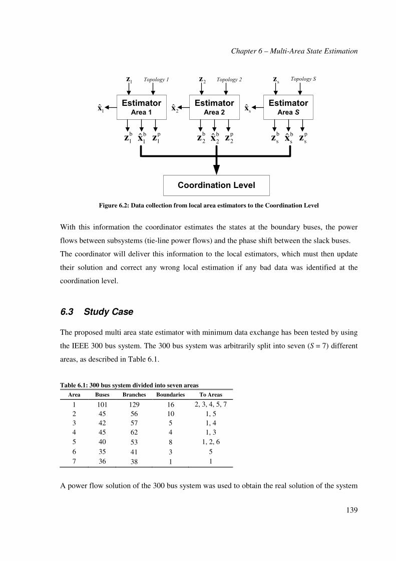
Figure 6.2: Data collection from local area estimators to the Coordination Level .................. 139
Figure 6.3: Boundary buses of Multi-Area System ................................................................. 140
Figure 6.4: Absolute angle error for boundary buses without PMU measurements ................ 145
Preface
6
Figure 6.5: Absolute voltage magnitude error for boundary buses without PMU measurements.................................................................................................................................................. 145
Figure 6.6: Absolute angle error for boundary buses including PMU measurements ............. 146
Figure 6.7: Absolute voltage magnitude error for boundary buses including PMU measurements ........................................................................................................................... 146
Figure 7.1: Structure of DSE ................................................................................................... 151
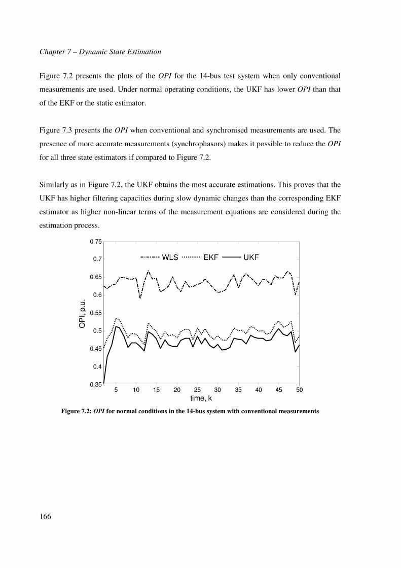
Figure 7.2: OPI for normal conditions in the 14-bus system with conventional measurements.................................................................................................................................................. 166
Figure 7.3: OPI for normal conditions in the 14-bus system with PMU measurements ......... 167
Figure 7.4: OPI calculation for sudden load change in 14-bus system with PMU measurements.................................................................................................................................................. 168
Figure 7.5: Skewness calculation for sudden load change in 14-bus system with PMU measurements ........................................................................................................................... 169
Figure 7.6: Normalised Innovation vector for sudden load change in 14-bus system with PMU measurements ........................................................................................................................... 169
Figure 7.7: OPI during bad data at k = 25, in the 57-bus system with PMU measurements ... 170
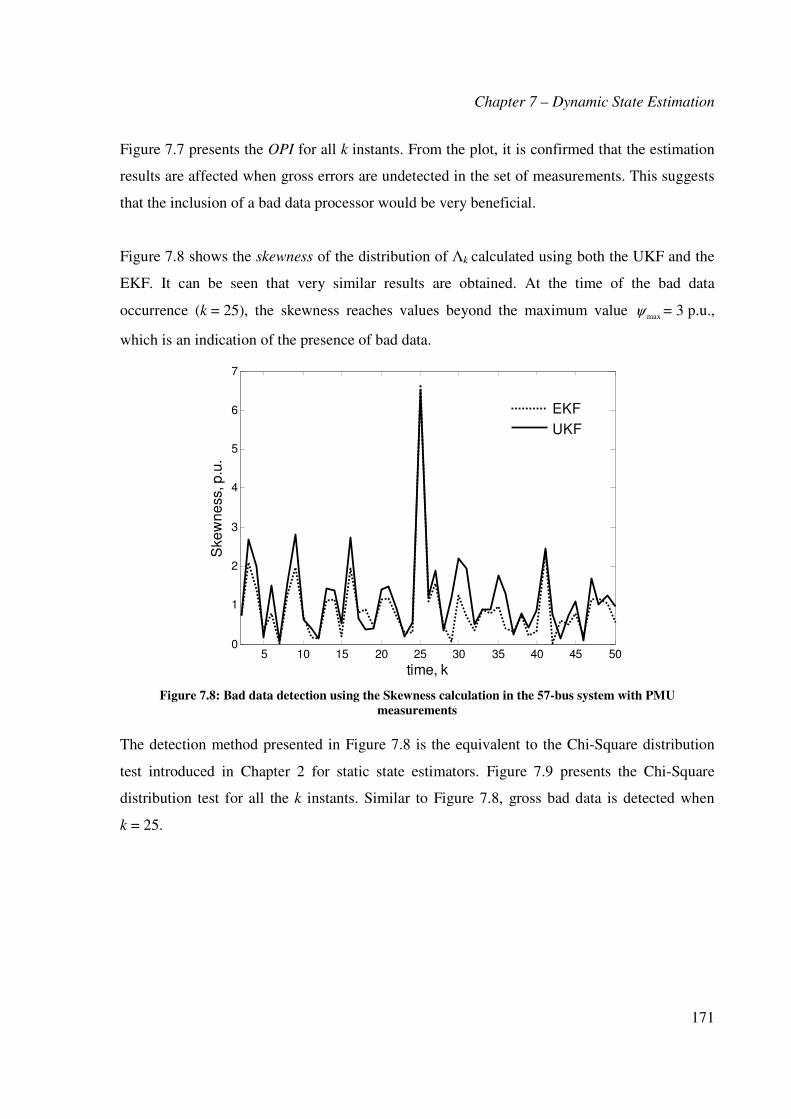
Figure 7.8: Bad data detection using the Skewness calculation in the 57-bus system with PMU measurements ........................................................................................................................... 171
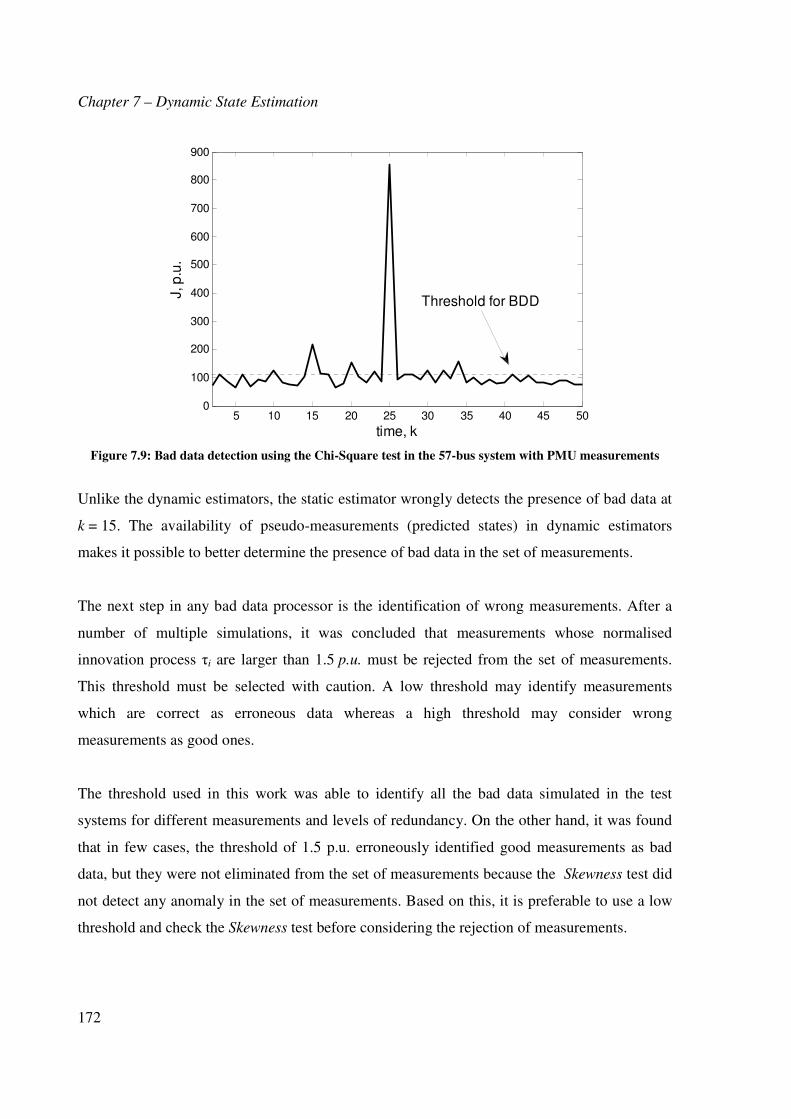
Figure 7.9: Bad data detection using the Chi-Square test in the 57-bus system with PMU measurements ........................................................................................................................... 172
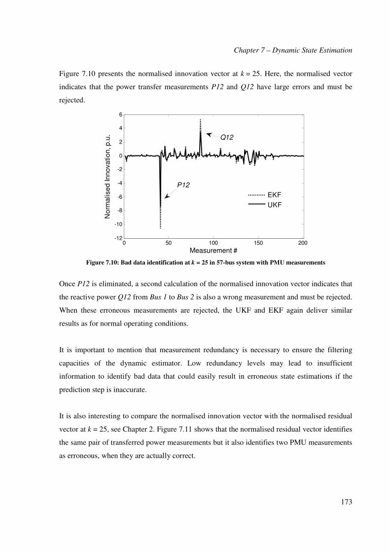
Figure 7.10: Bad data identification at k = 25 in 57-bus system with PMU measurements .... 173
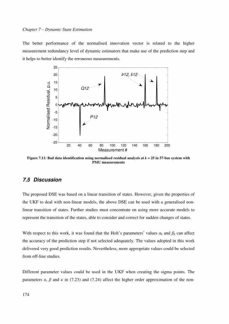
Figure 7.11: Bad data identification using normalised residual analysis at k = 25 in 57-bus system with PMU measurements ............................................................................................. 174
Figure 10.1: One Line Diagram 14-bus System ...................................................................... 205
Figure 10.2: One Line Diagram 57-bus System ...................................................................... 207
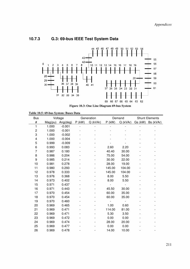
Figure 10.3: One Line Diagram 69-bus System ...................................................................... 211
Figure 10.4: One Line Diagram 118-bus System .................................................................... 215
Preface
7
List of Tables
Table 2.1: Elements of H corresponding to power injections .................................................... 28 Table 2.2: Elements of H corresponding to line power flows ................................................... 29 Table 2.3: Elements of H for bus voltages ................................................................................. 29 Table 3.1: Parameters of a Gaussian mixture distribution with seven components .................. 44 Table 3.2: Js
N for resulting gY(y) and the original mixture fY(y) ................................................. 54 Table 3.3: Comparison of computer time requirements ............................................................ 55 Table 3.4: Js
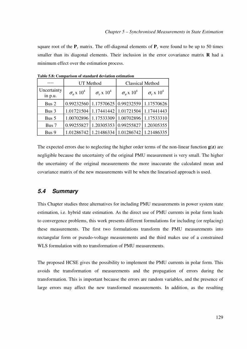
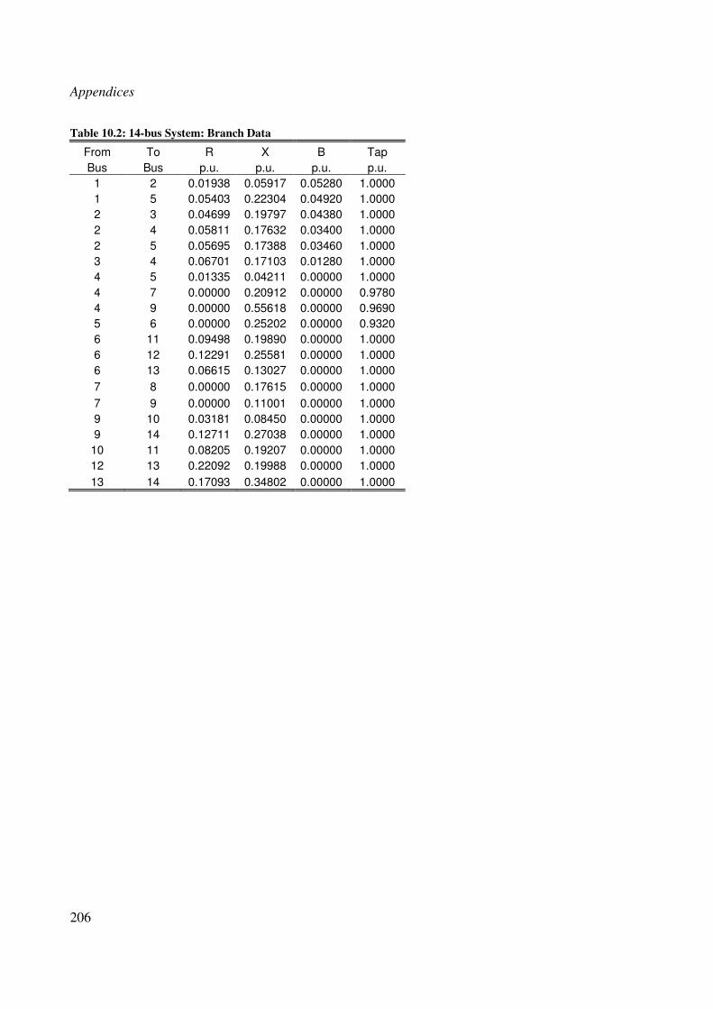
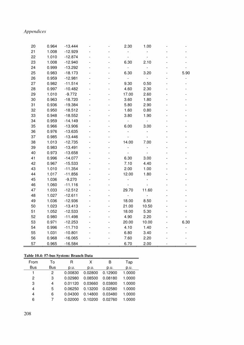
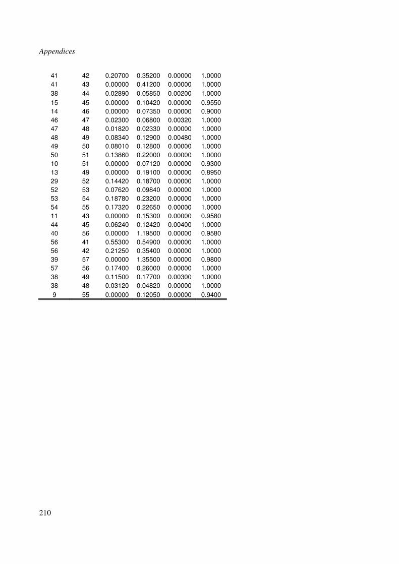
N for the resulting improved gY(y) and the original mixture fY(y) .......................... 58 Table 3.5: GMM parameters of variables to be correlated ........................................................ 61 Table 3.6: Estimated GMM parameters of correlated variables ................................................ 64 Table 4.1: GMM parameters of the non-Gaussian PDFs of active power injections (P) in p.u. 70 Table 4.2: Average value of percentage errors Case 1. ............................................................. 74 Table 4.3: Average value of percentage errors Case 2. ............................................................. 78 Table 4.4: GMM parameters of active power injections (P), in p.u. for 57-bus test system ..... 78 Table 4.5: Average value of percentage errors .......................................................................... 87 Table 4.6: Original parameters of GMM in radial network ....................................................... 88 Table 4.7: Average of estimation errors for radial network ....................................................... 97 Table 5.1: Elements of H corresponding to rectangular current measurements ...................... 110 Table 5.2: Elements of C corresponding to equality constraints of voltages ........................... 115 Table 5.3: Standard deviation of measurements ...................................................................... 119 Table 5.4: Optimal location of PMUs ...................................................................................... 123 Table 5.5: Estimation results for 100 Monte Carlo simulations .............................................. 127 Table 5.6: Time demands of hybrid estimators...................................................................... 128 Table 5.7: Comparison of mean vector estimation .................................................................. 128 Table 5.8: Comparison of standard deviation estimation ........................................................ 129 Table 6.1: 300 bus system divided into seven areas ................................................................ 139 Table 6.2: Standard deviation of measurement in 300 bus test system ................................... 140 Table 6.3: Chi-Square test for BDD without PMUs ................................................................ 141 Table 6.4: Chi-Square test for BDD including PMUs ............................................................. 141 Table 6.5: Percentage error of estimated active and reactive power flows.............................. 142 Table 6.6: Size of coordination level ....................................................................................... 144 Table 6.7: Assessment of coordination level ........................................................................... 144 Table 7.1: Performance indices during normal conditions for 14-bus test system .................. 165 Table 10.1: 14-bus System: Buses Data................................................................................... 205 Table 10.2: 14-bus System: Branch Data................................................................................. 206 Table 10.3: 57-bus System: Buses Data................................................................................... 207 Table 10.4: 57-bus System: Branch Data................................................................................. 208 Table 10.5: 69-bus System: Buses Data................................................................................... 211 Table 10.6: 69-bus System: Branch Data................................................................................. 213 Table 10.7: 118-bus System: Buses Data ................................................................................ 215 Table 10.8: 118-bus System: Branch Data .............................................................................. 218 Table 10.9: 300-bus System: Buses Data ................................................................................ 223 Table 10.10: 300-bus System: Branch Data............................................................................. 229
Preface
8
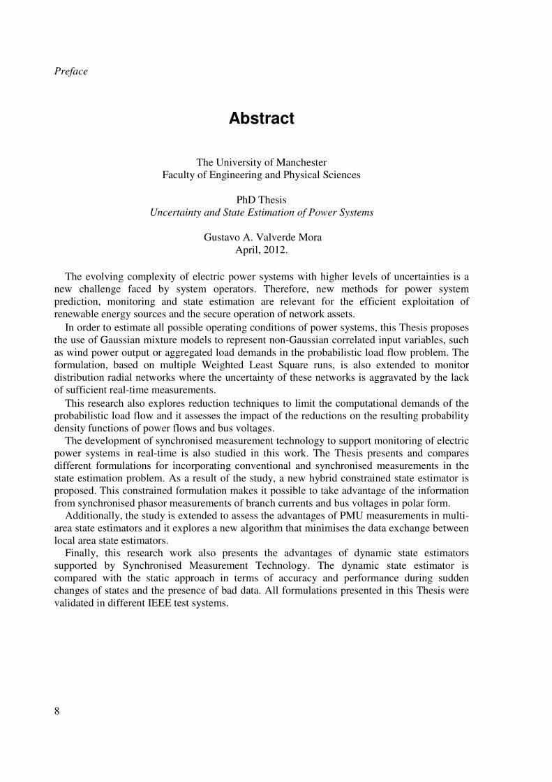
Abstract
The University of Manchester
Faculty of Engineering and Physical Sciences
PhD Thesis Uncertainty and State Estimation of Power Systems
Gustavo A. Valverde Mora
April, 2012.
The evolving complexity of electric power systems with higher levels of uncertainties is a new challenge faced by system operators. Therefore, new methods for power system prediction, monitoring and state estimation are relevant for the efficient exploitation of renewable energy sources and the secure operation of network assets.
In order to estimate all possible operating conditions of power systems, this Thesis proposes the use of Gaussian mixture models to represent non-Gaussian correlated input variables, such as wind power output or aggregated load demands in the probabilistic load flow problem. The formulation, based on multiple Weighted Least Square runs, is also extended to monitor distribution radial networks where the uncertainty of these networks is aggravated by the lack of sufficient real-time measurements.
This research also explores reduction techniques to limit the computational demands of the probabilistic load flow and it assesses the impact of the reductions on the resulting probability density functions of power flows and bus voltages.
The development of synchronised measurement technology to support monitoring of electric power systems in real-time is also studied in this work. The Thesis presents and compares different formulations for incorporating conventional and synchronised measurements in the state estimation problem. As a result of the study, a new hybrid constrained state estimator is proposed. This constrained formulation makes it possible to take advantage of the information from synchronised phasor measurements of branch currents and bus voltages in polar form.
Additionally, the study is extended to assess the advantages of PMU measurements in multi-area state estimators and it explores a new algorithm that minimises the data exchange between local area state estimators.
Finally, this research work also presents the advantages of dynamic state estimators supported by Synchronised Measurement Technology. The dynamic state estimator is compared with the static approach in terms of accuracy and performance during sudden changes of states and the presence of bad data. All formulations presented in this Thesis were validated in different IEEE test systems.
Preface
9
Declaration
No portion of the work referred to in the thesis has been submitted in support of an application
for another degree or qualification of this or any other university or other institute of learning.
Preface
10
Copyright Statement
i. The author of this thesis (including any appendices and/or schedules to this thesis) owns
certain copyright or related rights in it (the “Copyright”) and he has given The University
of Manchester certain rights to use such Copyright, including for administrative purposes.
ii. Copies of this thesis, either in full or in extracts and whether in hard or electronic copy,
may be made only in accordance with the Copyright, Designs and Patents Act 1988 (as
amended) and regulations issued under it or, where appropriate, in accordance with
licensing agreements which the University has from time to time. This page must form
part of any such copies made.
iii. The ownership of certain Copyright, patents, designs, trade marks and other
intellectual property (the “Intellectual Property”) and any reproductions of copyright works
in the thesis, for example graphs and tables (“Reproductions”), which may be described in
this thesis, may not be owned by the author and may be owned by third parties. Such
Intellectual Property and Reproductions cannot and must not be made available for use
without the prior written permission of the owner(s) of the relevant Intellectual Property
and/or Reproductions.
iv. Further information on the conditions under which disclosure, publication and
commercialisation of this thesis, the Copyright and any Intellectual Property and/or
Reproductions described in it may take place is available in the University IP Policy (see:
http://www.campus.manchester.ac.uk/medialibrary/policies/intellectual-property.pdf), in
any relevant Thesis restriction declarations deposited in the University Library, The
University Library’s regulations (see: http://www.manchester.ac.uk/library/aboutus/regulations)
and in The University’s policy on presentation of Theses
Preface
11
To my wife Rebeca and my parents
Preface
12
Acknowledgements
I want to thank God for giving me the opportunity to complete my studies and for all the
blessings I have received so far. I also want to thank my supervisor Prof. Vladimir Terzija for
his help during my PhD studies.
Special thanks to the Engineering and Physical Science Research Council (EPSRC) in the UK
and the University of Costa Rica (UCR) for their financial support during my PhD studies. I
am very pleased to be part of the School of Electrical Engineering in the UCR.
I want to express my gratitude to Dr. Elias Kyriakides, Dr. Saikat Chakrabarti, Prof. Gerald
Heydt and Prof. Andrija Saric for their helpful comments and guidance during my research
work.
Thanks to my friends and family in Costa Rica for their support and all my friends in
Manchester for making my life easier and funnier, particularly to Miguel, Ricardo, Manuel,
Gary, Deyu, Pawel, Jairo, Angel, Nando and Helge.
Special thanks to my parents Grettel Mora and Humberto Valverde for their support, love and
comprehension. You guys understood that I had a dream that today becomes true… I am sure
you are very proud about it.
Finally, I want to express my gratitude to my beloved wife Rebeca for being there always next
to me. Thanks for your comprehension and support during stressful moments of my studies. I
have no way to pay you back. Remember that this is also your PhD Thesis.
Chapter 1 - Introduction
13
Chapter 1 Introduction
The systematic interconnection of power systems that took place in the second half of the
twentieth century, as an attempt to strengthen the networks and to facilitate the transmission of
electricity, brought new operation challenges that could not be faced by power engineers unless
the state of the network was properly monitored in real-time [1].
The blackout of 1965 in the northeast region of the US encouraged power engineers to develop
sophisticated tools to collect, transmit and process measurements from all over the network for
the supervision and control of the system. This was a step before today’s Energy Management
Systems (EMS) of modern power networks. These EMS are in charge of the data acquisition,
state estimation, load flow analysis, economic dispatch, voltage-frequency control and security
assessment of the system, among other sophisticated features.
For many years, these tools were very effective to monitor and control power networks made
of conventional generation and uncongested transmission corridors. Today, the panorama has
changed:
• There is a need to reduce CO2 emissions of existing power plants which must be
gradually replaced by renewable generation, e.g. wind farms or solar panels.
• This renewable generation is variable, difficult to predict and no longer centralised but
distributed.
• The networks follow a deregulated structure to incentivise investment and efficiency in
electricity utilisation. Based on this,
• The networks operate closer to their stability limits and transmission corridors are
stressed due to the restrictions on the building of new transmission lines.
In order to cope with the challenges faced by intermittent generation, congested transmission
corridors and massive exchange of power between areas, it is necessary to improve the current
practice to monitor the power networks in real-time and to explore new tools that can be used
Chapter 1 - Introduction
14
to analyse the network operation over a range of possible conditions imposed by the
uncertainty of intermittent generation and demand.
1.1 Research Background
The following subsections present an introduction of previous work related to the topics
covered in this PhD Thesis. Further literature review is presented at the beginning of each
Chapter.
1.1.1 Probabilistic Load Flows
The Probabilistic Load Flow (PLF) studies are typically run for network planning purposes and
they analyse the performance of the power network over most of its working operation
conditions. The studies determine the likelihood of overstressed transmission corridors and
unacceptable bus voltage magnitudes and they can assess the impact of intermittent generation
in power networks [2].
The PLF takes into account the random nature of generation and demand, represented by
probability density functions, to determine the probability density of output variables such as
bus voltages and power flows. It was firstly proposed in [3] by Borkowska in 1974, and it can
be solved either numerically (e.g. Monte Carlo simulations) or analytically by mathematical
developments as an alternative to reduce the computational demands of the Monte Carlo
simulations [4].
Among the first analytical methods, Allan et al. solved the probabilistic load flow by linear
approximations of the power flow equations [5]. Here, the probability densities of the power
flows were approximated by convolution techniques.
In 1990, da Silva and Arienti combined the Monte Carlo Simulations and a multi-linearised
load flow equations in [6]. In addition, the Weighted Least Square (WLS) method was used in
Chapter 1 - Introduction
15
[7] to solve the PLF problem where all of the input variables were treated as Gaussian random
variables.
Recently in 2005, the Point Estimate method was implemented in probabilistic power flows
[8]. The method calculates a set of deterministic points to capture the first moments of the
input random variables. These points are later evaluated in the power flow problem to obtain
the mean and standard deviation of any power system variable.
An extension of the capabilities of the Point Estimate method was later presented in [9].
Normal and Binomial distributions were used to model the input variables. The authors
compared four Hong’s Point Estimate methods whose differences are the required number of
deterministic points. They found that for a large number of input random variables m, the
creation of 2m+1 points provides the best performance i.e. closer to the Monte Carlo
simulation results.
During the last few decades, the PLF studies were used to study the variability of aggregated
loads modelled by Gaussian distributions. With the increased penetration of intermittent
generation, the probabilistic studies have gained more attention due to the need for modelling
the intermittent power output as random variables that are typically non-Gaussian
distributed [10, 11].
Because of the proliferation of these renewable sources, the representation of these non-
Gaussian PDFs is an open field of research. Different approximations have been developed to
model non-Gaussian input random variables in power systems. For instance, in order to model
the variability of wind power output, an indirect algorithm based on the Beta distribution was
proposed in [12] and later considered in [10].
The probability distribution of the wind speed is typically non-Gaussian and it has been
modelled by the Gamma, Weibull or the Rayleigh distributions [4]. The Weibull distribution
has demonstrated better results because of its two flexible parameters k and c [13].
Nonetheless, since the wind speed PDF cannot be always approximated as a Weibull
Chapter 1 - Introduction
16
distribution, a mixed Gamma-Weibull distribution and a mixed truncated Normal distribution
were introduced in [13].
The PDFs of power demands of aggregated loads can be also non-Gaussian distributed. For
example, the Normal, log-normal and Beta distributions were used to evaluate their
effectiveness to model the load uncertainty [14]. Because of its flexibility to adapt to the
skewness of the distribution, the Beta distribution was found to be the most appropriate. This
distribution was also used in [15] to model the variability of load demand.
Recently, a more accurate approximation of the marginal distribution of any power demand
was introduced in [16]. As the PDF of load demands cannot be represented by a specific
distribution, the authors proposed the use of the Gaussian mixture distribution. Although the
work in [16] concentrates on the probability distribution of power demands, Gaussian mixtures
can be used to represent the variability of any other non-Gaussian variable in electric power
systems, e.g. renewable energy sources.
The present research work starts from the latter affirmation: it assumes that the marginal
distribution of any wind farm power output, wind speed or power demands can be represented
by Gaussian mixtures and this will be the input of the PLF analysis.
1.1.2 State Estimation
State Estimation is the process of assigning a value to an unknown system state variable based
on measurements collected from the network [17]. The state variables are the bus voltage
magnitudes and their phase angles and they are typically estimated by the WLS formulation.
The process involves redundant imperfect measurements that are processed to obtain the best
estimate of the system state. The state estimator acts as a filter block between the raw
measurements received from all over the network and the EMS applications that require very
accurate and reliable information about the actual state of the network [18].
Chapter 1 - Introduction
17
The typical sources of errors that affect the performance of modern state estimators are:
topology errors (undetected by the operator); gross errors in measurements and transducers;
parameter errors in the data base and the unsynchronised nature of conventional measurements.
However, the development of synchronised measurements units has opened new opportunities
to better monitor the power networks. The development of new strategies for incorporating
these synchronised measurements in current state estimators is one of the main objectives of
this Thesis.
1.1.3 Synchronised Measurements
A Phasor Measurement Unit (PMU) is a piece of equipment able to measure phasors of voltage
and currents, usually called synchrophasors. They were firstly introduced in the early 1980s
and they originally served as disturbance recorders [19].
The PMUs are the base line of wide-area monitoring systems that collect and process
synchronised measurements across the network to monitor power oscillations during large
disturbances and to monitor power flows and bus voltages during normal steady state
conditions [20].
In 2005, the IEEE published the Standard C.37.118-2005 to establish the data exchange
requirements in order to facilitate the compatibility of equipment between different
vendors [21]. Standard C.37.118-2005 also defines a list of steady state performance
requirements including range of signal frequency, phase angle, and harmonic distortion, among
others [22]. The performance of PMUs with dynamic measurements was not included in
C.37.118-2005 but it will be included in an updated version of C.37.118.
Since the PMUs can measure phasors of bus voltages, the state can be measured directly. This
is an advantage that could not be achieved by conventional unsynchronised measurements of
power flows. Additionally, as phasors of current can be measured, it is possible to extend the
voltage measurements to buses where no PMUs are installed.
Chapter 1 - Introduction
18
To date, the process of introducing PMUs in power systems is costly and it requires more time
to see the full benefits of wide area monitoring systems. In the meanwhile, the studies must
concentrate on making the most of the information provided by few installed PMUs until the
gradual insertion of PMUs will make the system fully observable.
1.1.4 Hybrid State Estimators
The use of synchrophasors improves the capability to monitor the condition of the system in
real-time. The inclusion of PMU measurements in existing state estimators increases the
redundancy levels for better bad data detection, helps to determine the actual topology of the
network and improves the accuracy of the estimation as synchronised measurements are
substantially more accurate than conventional measurements [23-26].
If a system becomes fully observable with only PMU measurements, a linear (non-iterative)
WLS can be used as direct measurements of voltage and current phasors are available.
However, the high cost of installing hundreds of PMUs in large interconnected power systems
makes this option unfeasible in the short term. As a consequence, a mixture of existing
conventional measurements and synchronised measurements is the most practical and feasible
option to gradually incorporate these synchronised measurements in existing estimators.
An example of this transition is the state estimator proposed in [26]. This state estimator
consists of a two-step state estimator: a conventional state estimator corrected by a linear state
estimator that uses synchronised measurements only. The main advantage of this estimator is
that there is no need to replace the existing conventional state estimator.
An alternative hybrid state estimator was later proposed in [27]. Unlike the two-step hybrid
estimator, the authors combined both the conventional and synchronised measurements in a
non-linear state estimator.
Recent studies also proposed new formulations for including synchrophasors in Multi-Area
State Estimators (MASE). It was found that synchrophasors can be used to improve bad data
Chapter 1 - Introduction
19
processing around boundary buses [28], and to measure the phase shift between the slack buses
of different areas [29, 30].
This Thesis, as extension of the work presented above, explores new methods for combining
conventional and synchronised measurements in modern state estimators, and assesses the
impact of the dispersed PMU measurements in single-area and multi-area state estimation. It
also explores the use of synchrophasors in dynamic state estimation.
1.2 Objectives
• To provide a step forward on probabilistic studies to estimate the operating conditions
of electric power systems in the presence of uncertain input variables such as power
demand and intermittent generation.
• To improve state estimation practice, enabling it to cope with the uncertainty of the
system to achieve a better network monitoring by making use of available technology
based on synchronised measurements.
• To propose and explore different formulations for including synchronised phasor
measurements in state estimation, including static and dynamic state estimators.
1.3 Thesis Structure
Chapter 1 – Introduction This is the introduction of the Thesis. This chapter presents a brief explanation of the
importance and relevance of this research work. In addition, the Chapter presents the objectives
and the contribution of this PhD Thesis.
Chapter 1 - Introduction
20
Chapter 2 – Classical State Estimation in Power Systems The Chapter presents an overview of power system state estimation theory including the details
of the WLS formulation, observability analysis, redundancy analysis and bad data processing.
It also introduces the equations of power flows and power injections that are used in the WLS
formulation. The theory presented in this Chapter is later implemented in the following
Chapters of the Thesis.
Chapter 3 – Estimation of Probabilistic Load Flows: Theory and Modelling This Chapter extends the Gaussian Component Combination Method (GCCM), originally
introduced in [31] as an alternative to Monte Carlo simulations, to estimate probability density
functions of power flows and bus voltages in the presence of non-Gaussian correlated random
input variables (papers 4 and 5 in Appendix H). Additionally, the use of Gaussian mixture
reduction techniques to limit the computational demand of the GCCM is proposed (Paper 9 in
Appendix H).
Chapter 4 – Estimation of Probabilistic Load Flows: Simulations
The probabilistic load flow study introduced in Chapter 3 is implemented in three
representative test systems. The study includes the impact of the correlation between input
variables in power flow studies of transmission networks and state estimation of distribution
networks (Papers 4 and 5 in Appendix H).
Chapter 5 – Synchronised Measurements in State Estimation
This Chapter explores different methods to include synchronised measurements in state
estimation based on the WLS formulation. The study focuses on how the PMU measurements
of currents can be used to improve the accuracy of hybrid state estimators.
Based on the inability to include current measurements in polar form, this study proposes the
use of a Hybrid Constrained State Estimator (HCSE) that avoids the propagation of
measurement uncertainties because it does not use any transformation of measurements. A
Chapter 1 - Introduction
21
comparison with other hybrid state estimators is included in the analysis (Paper 2 in
Appendix H).
Chapter 6 – Multi-Area State Estimation
This Chapter deals with the problem of state estimation in multi-area power systems. The study
proposes a Multi-Area State Estimator (MASE) based on wide area synchronised
measurements to estimate the angle difference between reference buses and to improve the
estimation accuracy in boundary buses.
The main objective of the proposed MASE is to reduce the data exchange between local area
and the coordination state estimators, and consequently to reduce the number of estimated
states of the coordination level. The impact of the proposed simplified MASE is also assessed
in terms of accuracy in a 300 bus test system (paper 6 in Appendix H).
Chapter 7 – Dynamic State Estimation
Due to the possibility to process scans of measurements with higher sampling rates, this
Chapter explores the use of power system dynamic state estimators supported by synchronised
measurements. In addition, this study explores the use of the Unscented Kalman Filter (UKF)
as an alternative to the Extended Kalman Filter (EKF) to cope with the non-linearities of the
measurement equations used in dynamic state estimators.
Finally, this Chapter compares the performance of dynamic and static estimators under normal
conditions, the presence of bad data and sudden changes of states. This study was implemented
in two test systems (paper 1 in Appendix H).
Chapter 8 – Conclusions and Future Work This Chapter summarises the conclusions drawn from the tests executed in Chapters 3
through 7. Furthermore, it discusses the limitations of the presented work and presents new
ideas for future work as consequence of this research.
Chapter 1 - Introduction
22
Figure 1.1 presents a diagram with the structure of the PhD Thesis to summarise the
organisation of the research work.
Figure 1.1: PhD Thesis Structure
1.4 Contribution of this Research
In order of appearance, the main contributions of this Thesis are:
• Proposal of a probabilistic load flow to estimate power flows and bus voltages in the
presence of non-Gaussian correlated input variables (demand and intermittent
generation). The proposed method uses the actual probability density functions as input
variables – represented as Gaussian mixtures.
Chapter 1 - Introduction
23
• Development of a methodology to run Monte Carlo simulations with Gaussian mixture
models as input variables.
• Simplification of Gaussian mixture models (with fewer components) to reduce the
computational demands of the proposed probabilistic load flow (and state estimator).
• Evaluation of the impact of including (or neglecting) the correlation between input
variables on the estimated probability densities of voltages and power flows of
transmission and distribution networks.
• Proposal of a state estimator for distribution networks that uses few real real-time
measurements and pseudo-measurements of power injections expressed by probability
densities. This state estimator not only provides the estimated mean values of any
variable but also calculates the corresponding density function of voltages, power flows
and power injections of poorly monitored areas.
• Assessment of the impact of the reduced models in the calculation of the probability
densities in both the probabilistic load flow and the state estimator.
• Proposal of a hybrid constrained state estimator that uses synchronised measurements
in polar form. This method avoids the propagation of measurement uncertainties as no
transformation of measurements is required.
• Application of the Unscented Transformation to calculate the propagation of
measurement uncertainties when synchronised measurements are transformed (from
polar to rectangular form or as pseudo-measurements of voltages).
• Proposal of a multi-area state estimator, supported by synchronised measurements,
which requires minimum data exchange between the local and coordination estimators.
• Assessment of the impact of not including power injection measurements of boundary
buses in two-level multi-area state estimators.
• Implementation of the Unscented Kalman filter in power system dynamic state
estimation supported by synchronised measurements.
• Comparison of dynamic versus static state estimators in the presence of bad data and
after sudden changes of states.
A list of the publications achieved as a result of the research carried out during this PhD project
has been included in Appendix H.
Chapter 2 – Classical State Estimation in Power Systems
24
Chapter 2 Classical State Estimation in Power Systems
Power system State Estimation (SE) is one of the most critical on-line applications necessary
for efficient Energy Management System (EMS) applications. The solution of a state estimator
is used as input for optimal power flow studies and contingency analysis and it is also used for
real-time security assessment to determine, and subsequently correct, unacceptable voltage and
power flow levels, to determine network losses, to alert network topology changes and to
monitor transferred power flows between areas.
The state estimator provides the best estimate of the system states (voltage angles and
magnitudes) commonly using the non-linear Weighted Least Square (WLS) technique based on
available measurements in the network.
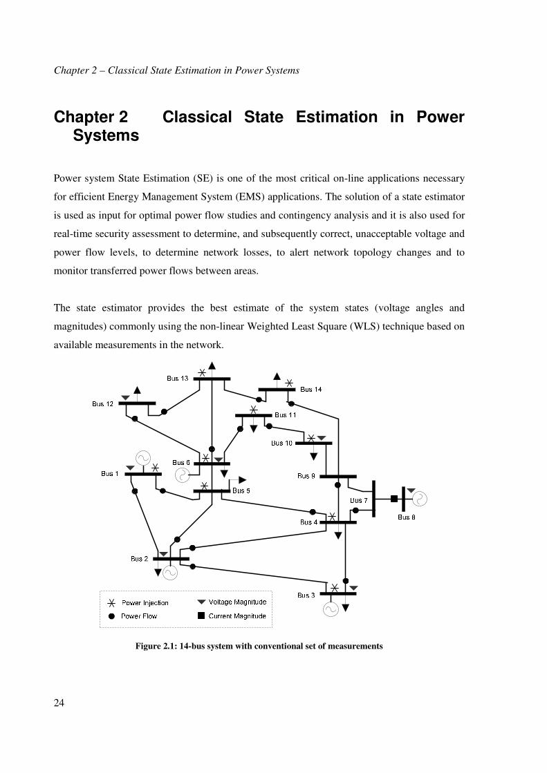
Figure 2.1: 14-bus system with conventional set of measurements
Chapter 2 – Classical State Estimation in Power Systems
25
Figure 2.1 presents an example of a small power system with dispersed conventional
measurements across the system which are commonly collected and transmitted through a
Supervisory Control and Data Acquisition (SCADA) system. These conventional
measurements and the set of virtual measurements (extended in Section 2.1.2.) are processed to
obtain the best estimate of voltages, power injections and power flows of directly and non-
directly monitored buses and transmission lines. The inclusion of more sophisticated, reliable
and synchronised measurements is presented in Chapters 5 to 7.
Figure 2.2 presents the functions of a SE [1]. In the pre-filtering step, the operator corrects and
eliminates measurements that are clearly wrong. The topology processor is implemented to
estimate the physical layout of substations and the connectivity between buses based on
information of Circuit Breaker (CB) status and available measurements.
The observability analysis is carried out to determine if the system state can be obtained from
the available set of measurements. In case the system is not fully observable, the SE determines
the unobservable zones/branches and the required set of measurements to make the system
fully observable.
Prefiltering
State Estimation
Error DetectionError
Identification
Observability
Analysis
Topology
Processing
Network
ParametersDynamic Data
Man-machine interface
Measurements
on/off switch indicators
and measurements
Errors Non-observable
zonesEstimated States
Figure 2.2: Building block of a state estimator
Chapter 2 – Classical State Estimation in Power Systems
26
The estimated states are obtained from the WLS method and it performs quite well under
quasi-steady state conditions. However, the good performance of the state estimator depends
on measurement accuracy and redundancy levels. Therefore, bad data detection and
elimination constitutes an important part of the state estimator.
The following sections present an overview of classical power system state estimation analysis
including the WLS formulation, observability analysis, redundancy analysis and bad data
processing. All the theory presented in this Chapter is later implemented in the following
Chapters of this Thesis.
2.1 WLS Formulation
The classical approach of state estimation in power systems consists of the application of the
Weighted Least Square (WLS) methodology, in which a set of measurements z can be
represented as [18]:
= + (2.1)
where h(x) is the set of equations relating the error free measurements with the state variables x
and e is the vector of uncorrelated measurement errors with mean value E[e] = 0. The n×1
state vector x is defined as the set of bus voltage magnitudes and angles. For instance, for an N-
bus system with reference at bus 1:
2 3 1 2[ , , , , , , , ]T
N NV V Vθ θ θ= ⋅⋅⋅ ⋅⋅⋅x (2.2)
Now let = − be a vector of residuals. The best estimate of x is the vector that
minimises the weighted sum of the squares of the measurement residuals r:
= − − (2.3)
where = ∙ = , , … , is the error covariance matrix and ! is the i-th
variance for the i = 1, 2,…, m measurements. The solution of (2.3) is obtained when the first
derivative of J , evaluated at the optimum state vector , gives a zero value.
Chapter 2 – Classical State Estimation in Power Systems
27
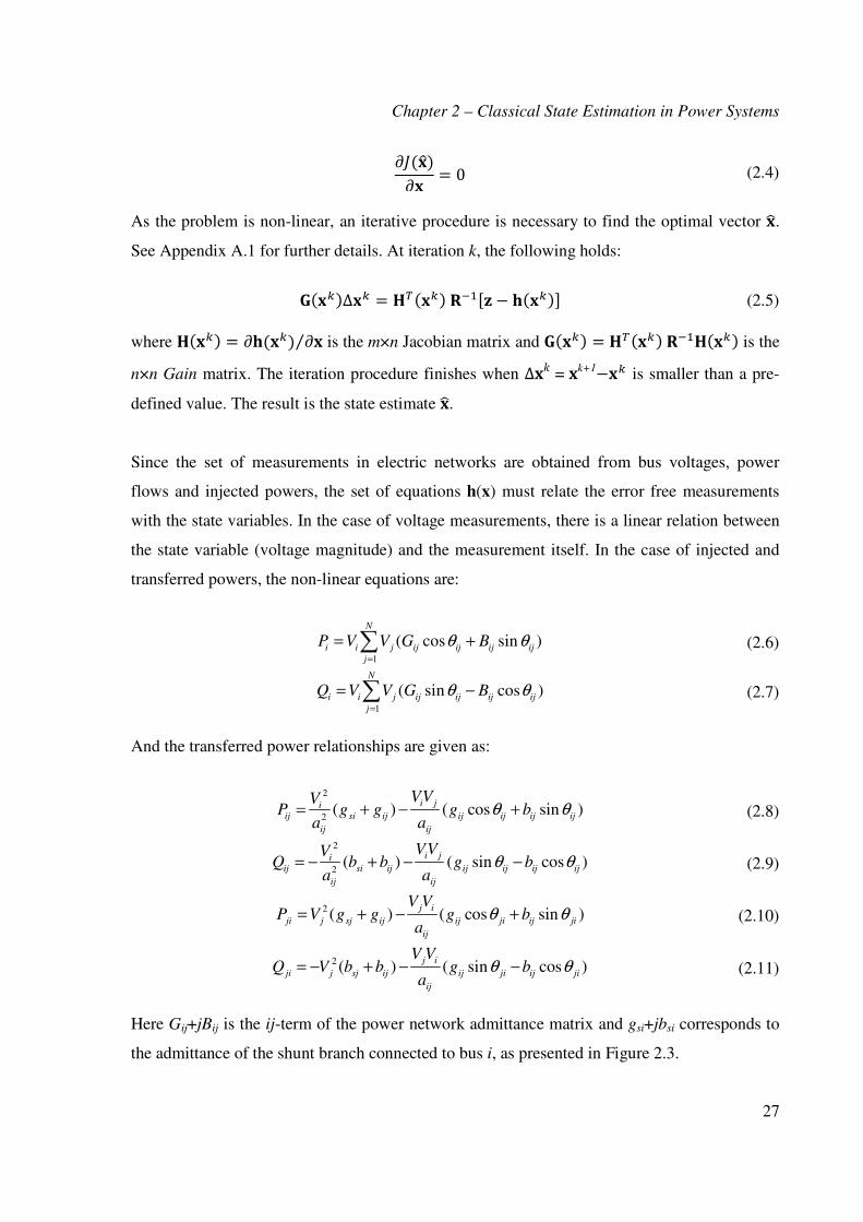
" #" = 0 (2.4)
As the problem is non-linear, an iterative procedure is necessary to find the optimal vector .
See Appendix A.1 for further details. At iteration k, the following holds:
%&∆& = (& − & (2.5)
where (& = "& "⁄ is the m×n Jacobian matrix and %& = (& (& is the
n×n Gain matrix. The iteration procedure finishes when ∆* = k+1−& is smaller than a pre-
defined value. The result is the state estimate .
Since the set of measurements in electric networks are obtained from bus voltages, power
flows and injected powers, the set of equations h(x) must relate the error free measurements
with the state variables. In the case of voltage measurements, there is a linear relation between
the state variable (voltage magnitude) and the measurement itself. In the case of injected and
transferred powers, the non-linear equations are:
1
( cos sin )N
i i j ij ij ij ij
j
P V V G Bθ θ=
= +∑ (2.6)
1
( sin cos )N
i i j ij ij ij ij
j
Q V V G Bθ θ=
= −∑ (2.7)
And the transferred power relationships are given as:
2
2( ) ( cos sin )
i ji
ij si ij ij ij ij ij
ij ij
VVVP g g g b
a aθ θ= + − + (2.8)
2
2( ) ( sin cos )
i ji
ij si ij ij ij ij ij
ij ij
VVVQ b b g b
a aθ θ= − + − − (2.9)
2 ( ) ( cos sin )j i
ji j sj ij ij ji ij ji
ij
V VP V g g g b
aθ θ= + − + (2.10)
2 ( ) ( sin cos )j i
ji j sj ij ij ji ij ji
ij
V VQ V b b g b
aθ θ= − + − − (2.11)
Here Gij+jBij is the ij-term of the power network admittance matrix and gsi+jbsi corresponds to
the admittance of the shunt branch connected to bus i, as presented in Figure 2.3.
Chapter 2 – Classical State Estimation in Power Systems
28
:1ij
aij ij
g jb+
i
( )si sig jb+ ( )sj sjg jb+
j
Figure 2.3: Pi-model of network branch including tap modelling
Also, aij is the off-nominal tap position of transformer connected to buses i and j. In case that
branch ij is a transmission line, aij = 1.
2.1.1 Jacobian Elements
The elements of the Jacobian matrix H(x) correspond to the partial derivatives of equations
(2.6) – (2.11) with respect to the state variables x, as presented in Tables 2.1 and 2.2. In
addition, the partial derivatives of the bus voltage magnitude with respect to the state variables
are presented in Table 2.3. Other types of measurements including synchronised and current
magnitude measurements will be presented in Chapter 5. The way how these measurements are
included and expressed in the SE is a key part of this work.
Table 2.1: Elements of H corresponding to power injections
2
1
( sin cos )N
ii j ij ij ij ij i ii
ji
PV V G B V Bθ θ
θ =
∂= − − −
∂∑
1
( cos sin )N
ij ij ij ij ij i ii
ji
PV G B V G
Vθ θ
=
∂= + +
∂∑
( sin cos )ii j ij ij ij ij
j
PVV G Bθ θ
θ
∂= −
∂ ( cos sin )i
i ij ij ij ij
j
PV G B
Vθ θ
∂= +
∂
2
1
( cos sin )N
ii j ij ij ij ij i ii
ji
QV V G B V Gθ θ
θ =
∂= + −
∂∑
1
( sin cos )N
ij ij ij ij ij i ii
ji
QV G B V B
Vθ θ
=
∂= − −
∂∑
( cos sin )ii j ij ij ij ij
j
QVV G Bθ θ
θ
∂= − +
∂ ( sin cos )i
i ij ij ij ij
j
QV G B
Vθ θ
∂= −
∂
Chapter 2 – Classical State Estimation in Power Systems
29
Table 2.2: Elements of H corresponding to line power flows
( sin cos )ij i j
ij ij ij ij
i ij
P VVg b
aθ θ
θ
∂= − − +
∂
22 ( ) ( cos sin )
ij jisi ij ij ij ij ij
i ij ij
P VVg g g b
V a aθ θ
∂= + − +
∂
( sin cos )ij i j
ij ij ij ij
j ij
P VVg b
aθ θ
θ
∂= − −
∂ ( cos sin )
ij i
ij ij ij ij
j ij
P Vg b
V aθ θ
∂= − +
∂
( sin cos )ji j i
ij ji ij ji
i ij
P V Vg b
aθ θ
θ
∂= − −
∂ ( cos sin )
ji j
ij ji ij ji
i ij
P Vg b
V aθ θ
∂= − +
∂
( sin cos )ji j i
ij ji ij ji
j ij
P V Vg b
aθ θ
θ
∂= − − +
∂ 2 ( ) ( cos sin )
ji ij sj ij ij ji ij ji
j ij
P VV g g g b
V aθ θ
∂= + − +
∂
( cos sin )ij i j
ij ij ij ij
i ij
Q VVg b
aθ θ
θ
∂= − +
∂
22 ( ) ( sin cos )
ij ji
si ij ij ij ij ij
i ij ij
Q VVb b g b
V a aθ θ
∂= − + − −
∂
( cos sin )ij i j
ij ij ij ij
j ij
Q VVg b
aθ θ
θ
∂= +
∂ ( sin cos )
ij i
ij ij ij ij
j ij
Q Vg b
V aθ θ
∂= − −
∂
( cos sin )ji j i
ij ji ij ji
i ij
Q V Vg b
aθ θ
θ
∂= +
∂ ( sin cos )
ji j
ij ji ij ji
i ij
Q Vg b
V aθ θ
∂= − −
∂
( cos sin )ji j i
ij ji ij ji
j ij
Q V Vg b
aθ θ
θ
∂= − +
∂ 2 ( ) ( sin cos )
ji i
j sj ij ij ji ij ji
j ij
Q VV b b g b
V aθ θ
∂= − + − −
∂
Table 2.3: Elements of H for bus voltages
0i
i
V
θ
∂=
∂ 1i
i
V
V
∂=
∂
0i
j
V
θ
∂=
∂ 0i
j
V
V
∂=
∂
2.1.2 Equality Constrained WLS
Even when the classical WLS method for state estimation provides reasonable results of power
injections at all buses, it may not provide a zero value for null power injections (no load or
generation connected). In order to improve the accuracy of the estimations, particularly around
the null power injection buses, a set of virtual measurements with mean value equal to zero and
small variance can be included in the formulation. However, the presence of very small
variances (large weights) in some measurements may lead to ill-conditioned Gain Matrix [18].
Chapter 2 – Classical State Estimation in Power Systems
30
Alternatively, a set of constraints can be included in the formulation to guarantee zero power
injections in those buses but also to avoid large weights in −1, which is one source of ill-
conditioning the Gain Matrix [18].
The minimization problem stated in equation (2.3) is now extended to meet a set of constraints
c(x) = 0. The Lagrange multipliers are used to account for the equality constraints as follows
[32, 33]:
,, -. = − − − -// (2.12)
where λc is the vector of Lagrange multipliers. Thus, partial derivatives of L(x, λc) with respect
to x and λc are obtained to minimise this function, see Appendix A.2 for details. Solving for
∆x and λc, it is possible to establish the iterative procedure to find the vector that minimises
L(x, λc):
0(& ( −1&−1& 2 3 0 ∆&
-.&43 = 0(& − &/& 3 (2.13)
where 1& = ∂/& ∂⁄ .
As seen from equation (2.13), the state vector is extended with a set of Lagrange multipliers.
Also, the Jacobian matrix is partitioned into a block corresponding to constraints and another
block related to all measurements in the system [33].
2.2 Observability Analysis
A power system is observable if the number of linearly independent measurements is equal or
larger than the number of states [1] . It means that for each state variable there must be at least
one measurement “observing” it. Reference [34] indicates in a simple way that a system is
observable if there are sufficient measurements to run a state estimator.
If one or more states are unobserved, the Gain Matrix G defined in (2.5) would become
singular, i.e. non invertible, and equation (2.5) could not be solved. Because of this, the system
is said to be unobservable due to insufficient number of measurements in the system.
Chapter 2 – Classical State Estimation in Power Systems
31
Two different concepts of observability are found in the literature [35]: Topological
Observability and Numerical Observability. The first one is based on Graph Theory, and the
second one is based on linear algebra formulation [36]. This research work focuses and applies
Numerical Observability as it also implies Topological Observability.
2.2.1 Numerical Observability
A system is said to be numerically observable if the Jacobian matrix is of full rank i.e. the
Gain Matrix is non-singular which is the condition for the state estimator to have a unique
solution.
A decoupled Jacobian matrix can be used to simplify the problem. The decoupling is based on
the fact that under normal operating conditions, changes of active powers are weakly related to
variations of magnitudes of bus voltages. In a similar way, changes of reactive powers are
weakly related to changes of bus angles [34].
The Jacobian matrix is approximated as:
0
0
P
QV
θ =
HH
H (2.14)
where ( , )
PPθ
∂=
∂
h V θH
θ and
( , )Q
QV
∂=
∂
h V θH
V. The subscripts P and Q refer to active and
reactive power equations, respectively. And the Gain Matrix will be:
V
θ
G 0G =
0 G (2.15)
where 1T
P P Pθ θ θ−=G H R H and 1T
V QV Q QV
−=G H R H . In other words, the observability of the system
can be obtained separately.
A power system with N buses is said to be P-θ numerically observable if the rank of Gθ, the
maximum number of linearly independent equations, is “N-1”. Also, the system is said to be Q-
V numerically observable if the rank of GV is “N” [37] . If the system is found to be P-θ
Chapter 2 – Classical State Estimation in Power Systems
32
numerically observable, it will be assumed to be Q-V numerically observable considering that
power measurements are obtained in pairs (active and reactive) and the existing of at least one
voltage magnitude measurement [38].
A linear model of the power measurements simplifies even more the problem to obtain the
factorization of the Gain Matrix Gθ. Since the numerical observability is independent of the
branch parameters and the operating state of the system, the voltage magnitudes at all buses
and the reactances at all branches are assumed to be 1 p.u.. Based on the previous assumptions,
the active power flow from bus i to j can be modelled as [39]:
ij i jP θ θ= − (2.16)
And the linear Jacobian matrix becomes:
0 1 1 0
i j
ij
P
Pθ
θ θ
− =
H
(2.17)
Here, the reference angle is also included in the set of states. Then, the Gain Matrix Gθ can be
easily decomposed using triangular factorization to obtain the new matrix θG . In case a zero
pivot is found during the factorization, it will be necessary to make permutation of rows in Gθ
and then continue with the decomposition.
If the system is not fully observable, more than one element will be zero in the diagonal of θG .
Otherwise, under full network observability, the last diagonal element of θG will be zero and
the rank of Gθ will be N-1. Note that, if one determines that the system is numerically
observable with the simplified linear model, one also ensures that the system is topologically
observable.
Chapter 2 – Classical State Estimation in Power Systems
33
2.2.2 Identification of Observable Islands
Based on a linear P-θ measurement model with unitary covariance matrix, the solution of the
estimated states, starting from (2.5), is:
ˆP Pθ =G θ H z (2.18)
where zP is the set of active power measurements. Consider the case where all the
measurements are all set to zero:
ˆθ =G θ 0 (2.19)
Under full network observability conditions, the estimated active powers obtained from (2.16)
should be also equal to zero. Any other value different from zero would imply that such branch
is not being observed with the available measurements.
From the decomposed matrix θG , it is possible to determine which branches are unobserved
and need measurement allocation. The algorithm is as follows [40]:
1. Initialize the measurement set with available measurements
2. Create the new gain matrix Gθ
3. Perform triangular factorization of Gθ (called θG ). A θ pseudo measurement is
introduced whenever a zero pivot is encountered. If only one zero pivot occurs
(necessary at the end), stop. Otherwise:
4. Solve the DC estimator from equation (2.18), considering all the measured values equal
to zero, except for the θ pseudo-measurements, that assume the values θk = 0, 1, 2 …
5. Evaluate the branch flows from equation (2.16).
6. Update the power network by removing all branches with Pij ≠ 0. These are
unobservable branches.
Chapter 2 – Classical State Estimation in Power Systems
34
7. Update the measurements set of interest by removing power injection measurements
from buses adjacent to at least one of the branches removed in Step 6. These are
irrelevant measurements.
8. Return to Step 2.
The iteration is required because the sub networks identified can only be theoretically
classified as candidate for observable islands [34]. Once all the unobserved branches are
removed, it is possible to identify all observable islands in the system. Allocation of new
measurements will be necessary to unify the observable islands and make the system fully
observable.
On the other hand, reference [41] uses a non-iterative numerical method to remove the non-
observable branches. From the decomposition of matrix Gθ, it is obtained the factors L (non-
singular unitary lower triangular matrix), and U (upper triangular matrix) such that Gθ = LU.
The decomposition is based on Gaussian elimination by using the Peters and Wilkinson
method explained in [42], see Appendix B.1.
Later, a singular diagonal matrix D is built up from D = L-1Gθ L
-T containing zero diagonal
elements in those rows corresponding to the zero pivots found during the factorization of Gθ.
By taking the inverse of L, and keeping the rows of L-1 corresponding to the zero diagonals of
D, it is obtained a Test Matrix W.
Finally, compute C matrix from the branch-bus incidence matrix A and matrix W:
T=C AW (2.20)
where the entry Aij is 1 (-1) if the sending (receiving) end of branch i connects to bus j, or zero
otherwise. If at least one element in a row of C is non-zero, then the corresponding branch is
unobservable. The observable islands are found once these branches are removed.
Chapter 2 – Classical State Estimation in Power Systems
35
2.3 Redundancy Analysis
In power system state estimation, a measurement can be classified as either critical or
redundant [39]. Redundant measurements can be removed from the system without causing
loss of observability. However, the removal of a critical measurement makes the system
unobservable. This is equivalent to say that the removal of a critical measurement decreases
(by one) the rank of the Jacobian Matrix H. The row of the Jacobian matrix corresponding to a
critical measurement is linearly independent of the other rows (other measurements) of H [43].
The residual ri =zi-hi() of any critical measurements i, is always zero (irrespective of good or
bad data) which means that any error in a critical measurement can not be detected, affecting
the performance of the state estimator [18].
A critical pair is a set of two measurements that when removed make the system unobservable,
a critical trio is a set of three measurements that when removed makes the system unobservable
and so on. An optimal placement of measurements can eliminate any critical measurement and
improve local redundancy levels (can eliminate critical pairs or trios).
Similar to Observability Analysis, the decoupled Jacobian matrix, based on a linear model of
the power measurements, is enough to identify critical measurements and redundancy levels.
The first step consists on the decomposition of the Jacobian matrix by using LU decomposition.
The set of measurements in the Jacobian matrix will include only the linear model of all
available real power measurements. The set of states are the bus phase angles but excluding the
reference bus.
After decomposition of PθH (and possible needed exchange of rows), the equivalent matrix
becomes [39]:
( 1)
( -1)
N
m N
red
−
×
=
IH
K (2.21)
where,
Chapter 2 – Classical State Estimation in Power Systems
36
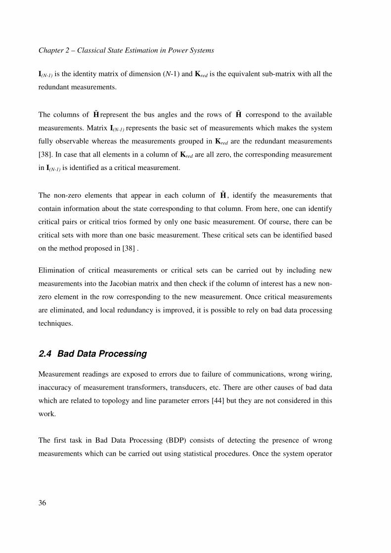
I(N-1) is the identity matrix of dimension (N-1) and Kred is the equivalent sub-matrix with all the
redundant measurements.
The columns of H represent the bus angles and the rows of H correspond to the available
measurements. Matrix I(N-1) represents the basic set of measurements which makes the system
fully observable whereas the measurements grouped in Kred are the redundant measurements
[38]. In case that all elements in a column of Kred are all zero, the corresponding measurement
in I(N-1) is identified as a critical measurement.
The non-zero elements that appear in each column of H , identify the measurements that
contain information about the state corresponding to that column. From here, one can identify
critical pairs or critical trios formed by only one basic measurement. Of course, there can be
critical sets with more than one basic measurement. These critical sets can be identified based
on the method proposed in [38] .
Elimination of critical measurements or critical sets can be carried out by including new
measurements into the Jacobian matrix and then check if the column of interest has a new non-
zero element in the row corresponding to the new measurement. Once critical measurements
are eliminated, and local redundancy is improved, it is possible to rely on bad data processing
techniques.
2.4 Bad Data Processing
Measurement readings are exposed to errors due to failure of communications, wrong wiring,
inaccuracy of measurement transformers, transducers, etc. There are other causes of bad data
which are related to topology and line parameter errors [44] but they are not considered in this
work.
The first task in Bad Data Processing (BDP) consists of detecting the presence of wrong
measurements which can be carried out using statistical procedures. Once the system operator
Chapter 2 – Classical State Estimation in Power Systems
37
knows that bad data are present in the set of measurements, it is necessary to eliminate it or
correct the bad data from other available information.
2.4.1 Chi square Distribution Test
Consider a set of independent random variables grouped in a vector v. If each element vi
follows a normal standard distribution N(0,1), the chi square distribution 2
mχ , with m degrees
of freedom, is the distribution of the random variable y defined as [18], [45]:
2
i
i=1
m
y v=∑ (2.22)
The degrees of freedom m represent the number of independent variables in the sum of squares.
This value will decrease if any of the variables vi form a linearly dependent subset.
Figure 2.4 presents the Probability Density Function (PDF) for a chi square distribution with
20 degrees of freedom. As the number of degrees of freedom m increases, the PDF of χ2 will
tend to a normal distribution [45].
Figure 2.4: Chi Square PDF for 20 degrees of freedom
The larger area under the PDF of Figure 2.4 represents the probability of finding a value of y
smaller than a threshold y1. Figure 2.4 shows that the probability of finding y smaller than 31.4
0 10 20 30 40 500
0.01
0.02
0.03
0.04
0.05
0.06
0.07
y
Chi S
quare
Dis
trib
ution
Area = 5%y1
Chapter 2 – Classical State Estimation in Power Systems
38
is 95%. This probability calculation can be used to detect presence of bad data in the set of
measurements.
If there is no bad data in the set of power system measurements and the m measurement errors
ei (i=1, 2, …, m) have normal distribution N(0, 2
iσ ), the performance index J( x ), defined in
equation (2.3), will follow a chi-square distribution χ2m-n. Here, m is the number of
measurements, n is the number of states and vector x refers to the estimated states [46]. The
degrees of freedom must be constrained to m-n because it is considered that there are at the
most m-n linearly independent equations.
One can determine that J( x ) follows a chi square distribution, i.e. free of bad data, if J( x ) is
smaller than a threshold y1 at a certain level of confidence α. This level of confidence α is
usually specified at 95% but may change depending on the system or application. Using the
example of Figure 2.4, if the estimated J( x ) for a given system with 20 degrees of freedom is
smaller than 31.4, bad data will not be suspected with a confidence level of 95%.
2.4.2 Measurement Residuals
This section introduces the identification of bad data based on the measurement residuals
approach [18]. Consider the linearized measurement equation around the estimated point x0:
∆ ∆z = H x + e (2.23)
where z = z-h(x0) is the mismatch between the measurement vector and its calculated value at
an estimate x0. Also x = x-x0, 0( )∂ ∂H = h x x and e is the set of uncorrelated measurement
errors with Gaussian distribution and covariance matrix R. Similar to (2.5), the WLS
estimation solution of the linearized state vector will be:
1 1 1ˆ ( )T T− − −∆ ∆x = H R H H R z (2.24)1 1ˆ T− −∆ ∆x = G H R z (2.25)
Chapter 2 – Classical State Estimation in Power Systems
39
And the estimated value of z will be:
ˆ ˆ∆ ∆ = ∆z = H x K z (2.26)
where 1 1T− −=K HG H R .
For a set of m measurements, the m × 1 vector of measurement residual will be denoted as:
ˆ= ∆ − ∆r z z (2.27)
( )= − ∆r I K z (2.28)
where I is the Identity Matrix. By substitution of equation (2.23) into (2.28) it is obtained:
( )( )= − ∆ +r I K H x e (2.29)
Based on the property that (I-K)H = 0, equation (2.29) can be expressed as [18], [44] :
( )= −r I K e (2.30)
=r Se (2.31)
Matrix S is called the Residual Sensitivity Matrix. Based on the relation above, it is possible to
calculate the probability distribution of the measurement residuals as follows:
( ) ( ) ( ) 0E E E= = =r Se S e (2.32)
cov( ) [ ]TE= =Ω r rr (2.33)
[ ]T TE=Ω S ee S (2.34)
T= =Ω SRS SR (2.35)
The off diagonal elements of the m × m matrix Ω identify strong versus weakly interacting
measurements. The higher the element Ωij, the stronger the interaction between measurements i
and j.
The covariance matrix Ω is also used to calculate the normalized residuals to identify and
reject any bad data in the set of measurements.
Chapter 2 – Classical State Estimation in Power Systems
40
2.4.3 Normalized Residual Test
Once the state estimation is obtained using WLS, the residual vector is calculated as the
difference between each measurement and the corresponding function h( x ):
ˆr = z - h(x) (2.36)
The normalized residuals are obtained by dividing its absolute value by the corresponding
diagonal entry in the residual covariance matrix Ω [45], [46]:
iN
i
ii
rr =
Ω (2.37)
Once the normalized residuals are obtained for all the measurements, the largest normalized
residual is compared with a pre-defined threshold. If this value is larger than the threshold, the
corresponding data will be removed and a new estimation is performed. This procedure is
repeated until the largest normalized residual is lower than the threshold previously
established.
If the value of the threshold is too small, the program would filter data that may not be wrong,
reducing redundancy, and it may lead to unobservable conditions. However, if the threshold is
large, it is possible that wrong data is still present. Generally, a threshold value of 3.0 is enough
to reject gross errors in the set of measurements.
There is a different approach where the bad data is not rejected at all but it is corrected instead.
This is achieved by subtracting the estimated error from the identified bad measurement.
However, this method may not be accurate enough for large errors [45]. The measurement
residual of the identified bad measurement is:
bad bad ˆ( )i i ii i
r z h S e= ≈- x (2.38)
By solving for ei:
1 bad
i i
ii
e rS
≈ (2.39)
Chapter 2 – Classical State Estimation in Power Systems
41
And subtracting this estimated error from the identified bad measurements yields:
1bad bad
i i i
ii
z z rS
≈ − (2.40)
The normalized residual approach is generally very effective but its main limitations are listed
below:
• It can not identify errors in critical measurements because the corresponding column in
S is zero. So, an error in that measurement could not be detected since it will have no
effect on the measurement residual [47] . Here the importance of having high redundant
systems.
• It may fail to identify erroneous measurements when two interacting measurements
have errors that are in agreement (multiple interacting and conforming bad data) [18].
2.5 Summary
This chapter introduced the classical techniques applied to state estimation, redundancy
analysis, observability analysis and bad data detection and elimination. The chapter also
presented the equations of power flow and power injection as function of the state variables
that are used in the WLS formulation. The following chapters will make reference to the
equations and formulations presented in Chapter 2.
Chapter 3 – Estimation of Probabilistic Load Flows: Theory and Modelling
42
Chapter 3 Estimation of Probabilistic Load Flows: Theory and Modelling
The insertion of intermittent wind power generation at the transmission level has increased the
level of uncertainty of the power networks. Distributed generation and emerging technologies
such as storage devices will also increase the uncertainty of the aggregated loads. This leads to
running stochastic/probabilistic studies where the input variables can no longer be treated as
deterministic values, but as stochastic ones [48].
Probabilistic load flow studies take into account the random nature of generation and demand
for a certain period. The information obtained from the probabilistic load flows can be used for
planning purposes when power engineers need to make decisions in terms of investment or for
operation purposes when it is needed to determine all the possible operating conditions of the
power system for a short period [49]. These studies provide valuable information about the
likelihood that certain bus voltage or power flow/injection will remain within some acceptable
limits.
Most of the work mentioned in Section 1.1.1 was concentrated on the uncertainty of power
injections, which were usually assumed to be Gaussian distributed with 5% to 10% of
variability. Recent studies have shown that the marginal distribution of wind power production
has larger variability and it is non-Gaussian distributed [4, 10].
Reference [31] uses a weighted sum of Gaussian distributions to model any non-Gaussian
distribution. The method uses multiple WLS runs to deal with the Gaussian components for
each non-correlated input variable.
To date, little attention has been paid to non-Gaussian correlated input variables. This is,
however, the most general and realistic scenario to be considered in probabilistic load flows
studies. Examples of non-Gaussian correlated variables are power demands of aggregated loads
with similar consumption patterns or wind/solar generation in the same geographic area.
Chapter 3 – Estimation of Probabilistic Load Flows: Theory and Modelling
43
References [2, 50] introduced non-Gaussian correlated variables to represent the stochastic
power output of wind farms in probabilistic power flows studies. The statistical moments were
estimated using the Point Estimate method and the Probability Density Functions (PDFs) were
approximated with the Cornish–Fisher expansion series.
In this work, the non-Gaussian PDFs are approximated by the Gaussian Mixture Model
(GMM), which is able to model any marginal distribution (standard or not) with a finite
number of components.
The contribution of this work is to extend the Gaussian Component Combination Method
(GCCM) introduced in [31] to estimate the PDF of power flows in presence of non-Gaussian
correlated random input variables.
The advantage of this approach is that it does not need any expansion series to approximate the
resulting PDF of the system variables. The resulting PDF of any electrical variable is made of
Gaussian components extracted from multiple WLS runs. As the number of WLS runs depends
only on the number of Gaussian components of the input variables, a Gaussian mixture
reduction technique is also proposed to limit the number of WLS runs.
The first part of this chapter introduces the Gaussian mixture distribution and the Gaussian
Mixture Model (GMM) to represent non-Gaussian random variables. Section 3.2 explains a
methodology to reduce the number of Gaussian components to simplify the GMMs.
Subsequently, Section 3.3 presents the Monte Carlo simulations and the Gaussian Component
Combination Method (GCCM) for probabilistic load flow studies in the presence of non-
Gaussian correlated variables, whereas Section 3.4 presents the summary of the Chapter.
3.1 Gaussian Mixture Distribution
A Gaussian mixture distribution is the mixture of L Gaussian distribution components. For a
one-dimensional random variable Y, the probability density function fY(y) is defined as [31]:
Chapter 3 – Estimation of Probabilistic Load Flows: Theory and Modelling
44
2( , )1
( ) ( )i i
L
Y i Ni
f y f yµ σω=
=∑ (3.1)
where ωi, µi and 2
iσ are the proportion, mean, and variance of the i-th component of the
Gaussian mixture, respectively. In order to maintain the characteristics of a probability
distribution, the proportions parameters are constrained to be:
1
0 1 and 1L
i i
i
ω ω=
< ≤ =∑ (3.2)
In addition, the distribution of the i-th Gaussian component is [51]:
2
2
2
( )
2
( , ) 2
1( )
2
i
i
i i
y
N
i
f y e
µ
σ
µ σπσ
− −
= . (3.3)
The mean and variance of the random variable are respectively [52]:
1
L
Y i i
i
µ ω µ=
=∑ (3.4)
( )2 2 2
1
( )L
Y i i i Y
i
σ ω σ µ µ=
= + −∑ (3.5)
The probability density of the Gaussian Mixture is obtained by evaluating fY(y) for ־∞ < y < ∞.
For example, consider a Gaussian mixture distribution (L = 7) with the parameters given in
Table 3.1:
Table 3.1: Parameters of a Gaussian mixture distribution with seven components
Component i=1 i=2 i=3 i=4 i=5 i=6 i=7
ωi 0.20 0.20 0.20 0.20 0.10 0.05 0.05
µi 43.0 50.0 52.0 58.0 62.0 72.0 80.0
σi2
9.0 16.0 9.0 64.0 4.0 4.0 25.0
Figure 3.1 presents the probability density of the variable Y modelled by the Gaussian mixture
parameters of Table 3.1. The sum of the individual weighted Gaussian components creates the
Gaussian mixture distribution. This variable Y represents any random variable such as power
demands, generation power outputs, or bus voltage magnitudes for a certain period. From
Figure 3.1, it can be concluded that the PDF of the variable Y is non-Gaussian and that it does
not fit any other typical marginal distribution.
Chapter 3 – Estimation of Probabilistic Load Flows: Theory and Modelling
45
Figure 3.1: Gaussian mixture distribution with 7 Gaussian components
The Cumulative Distribution Function (CDF) of the random variable is the probability that Y
assumes a value in the range −∞ < Y ≤ y [51]:
( ) Prob( ) ( )
y
Y YF y Y y f u du−∞
= ≤ = ∫ (3.6)
Figure 3.2 presents the CDF of the seven components Gaussian mixture with the parameters
listed in Table 3.1. The values of FY(y) represent probabilities and they lie in the range 0 to 1.
This is particularly important when creating Gaussian mixture random variables for Monte
Carlo simulations.
The main advantage of the Gaussian Mixture distribution is that it can approximate any PDF
with a finite number of components. This is of particular interest when the distribution of the
random variable does not fit the typical distributions (e.g. Gaussian, Uniform, Gamma, etc).
The higher the number of components of the Gaussian Mixture Model (GMM), the more
accurate the approximation becomes.
The most effective methodology to determine the GMM that best approximates the distribution
of the samples of Y is the Expectation Maximisation (EM) algorithm. For example, reference
30 40 50 60 70 80 900
0.01
0.02
0.03
0.04
0.05
0.06
variable Y
Pro
ba
bility D
en
sity
Components
Gaussian Mixture Distribution
Chapter 3 – Estimation of Probabilistic Load Flows: Theory and Modelling
46
[16] uses the EM algorithm to determine the parameters of the GMM to model PDFs of power
demands.
Figure 3.2: CDF for Gaussian mixture with seven components
The input of the EM algorithm is the set of samples γ = [y1, y2,…, ys] of the random variable Y
and the desired number of Gaussian components of the GMM. Given γ and the initial (or
updated) Gaussian mixture parameters η, the algorithm computes the expectation of the log-
likelihood of the complete data with respect to the unknown samples. Later, η is updated to
maximise the log-likelihood expectation found before. This procedure is iteratively executed
until convergence is achieved. The Statistics Toolbox of MATLAB offers the function
gmdistribution.fit to estimate η using the EM algorithm given the samples γ and the desired
number of Gaussian components [53].
Figure 3.3 presents the GMM of a Uniform random variable approximated by 10 components
using the EM algorithm. In fact, the Uniform distribution is one of the most difficult
distributions to approximate with a GMM. The approximation can be improved with a higher
number of Gaussian components.
30 40 50 60 70 80 90 1000
0.1
0.2
0.3
0.4
0.5
0.6
0.7
0.8
0.9
1
Cu
mu
lative
De
nsity
variable Y
Chapter 3 – Estimation of Probabilistic Load Flows: Theory and Modelling
47
Figure 3.3: Uniform distributed random variable modelled by GMM
Figure 3.4 presents the GMM approximation of a Gamma distributed random variable with 10
components. In this case, the mismatch between the GMM and the random variable density is
negligible.
Figure 3.4: Gamma distributed random variable modelled by GMM
20 30 40 50 60 700
0.005
0.01
0.015
0.02
0.025
0.03
0.035
0.04
variable Y
Pro
ba
bility D
en
sity
Normalised histogram bin
GMM with 10 components
0 5 10 15 20 25 30 350
0.05
0.1
0.15
variable Y
Pro
ba
bility D
en
sity
Normalised histogram bin
GMM with 10 components
Chapter 3 – Estimation of Probabilistic Load Flows: Theory and Modelling
48
The number of components needed to approximate any probability density function depends on
the degree of required accuracy. Although adding an extra component to the GMM will always
improve the approximation, the number of components is sufficient when adding an extra
component produces a negligible improvement in the approximation. The Chi-Square goodness
of fit test can be used to quantify the degree of fitness of the set of samples and the GMM [16].
By using a pre-defined threshold, it is possible to determine the number of components of the
GMM.
3.2 Reduction of Gaussian Mixtures
The number of components may be a limitation when dealing with simulations that involve a
large number of GMM at the same time. Based on this, it is very useful to decrease the number
of components of the mixtures in order to reduce the computation demands while keeping a
good level of accuracy of the original GMMs.
If one starts from the simplest GMM to represent a non-Gaussian variable and then increases
the number of components, it would be necessary to run the Expectation Maximisation (EM)
(fitting) technique each time it is desired to improve the accuracy of the GMM. This is both
time consuming and impractical. The proposed reduction method no longer requires the use of
the raw data (observations). Instead, it starts from the actual accurate model parameters of the
GMM and then reduces one component at a time.
The idea of the Gaussian mixture components reduction is to approximate the original GMM in
(3.1) as a new GMM with fewer components:
2( , )1
( ) ( )j j
M
Y j Nj
g y f yµ σω=
=∑ (3.7)
where M < L and jω , jµ and 2
jσ are the proportion, mean, and variance of the j-th component,
respectively.
Different reduction algorithms have been presented in recent years. The main requirements of a
good reduction algorithm can be summarised as [52]:
Chapter 3 – Estimation of Probabilistic Load Flows: Theory and Modelling
49
• The algorithm should be efficient and easy to execute.
• The algorithm should maintain the mean and variance of the original mixture. If not,
the deviation should be negligible.
• The resulting GMM should maintain, within some acceptable limits, the structure of
the original mixture.
These requirements may not all be achieved with one single algorithm but it is possible to
choose one algorithm or a mixture of algorithms that can achieve most of the requirements
listed above.
The approach based on merging pairs of components is the simplest method to reduce
Gaussian mixture components. The algorithm starts with gY(y) = fY(y). The merging is applied
to the pair of components of gY(y) that when merged produce the minimum discrepancy
between fY(y) and gY(y) [54], [55].
Once the pair of components i and j are identified, they are merged together to obtain a new
resulting component ij with the following component parameters [55]:
ij i jω ω ω= + (3.8)
The mean and variance of the new Gaussian component is:
( )1ij i i j j
i j
µ ω µ ω µω ω
= ++
(3.9)
2 2 2 21( )
i j
ij i i j j i j
i j i j
ω ωσ ω σ ω σ µ µ
ω ω ω ω
= + + − + +
(3.10)
The new component ij replaces the i-th and j-th components previously identified.
Consequently, gY(y) loses one component but keeps the mean and variance of the original
mixture. This procedure is repeated until the desired number of components is reached.
The identification of the i-th and j-th components of gY(y) depends on the selection criteria. The
Salmond method identifies the pair of components i and j that produce the minimum increase
of the first summand in (3.5) [56]. The increase of the first summand in (3.5) is related to the
Square Distance (SD) measure:
Chapter 3 – Estimation of Probabilistic Load Flows: Theory and Modelling
50
2
2
2
( )i j i j
ij
i j Y
dω ω µ µ
ω ω σ
−= ⋅
+
(3.11)
The smallest squared distance identifies the merged components i and j that produce the
minimum value of the cost function. The main disadvantage of this methodology is that it
merges the pair of components with the closest means even if their variances are very
different [55].
The Williams method identifies the pair of components to be merged that produce the
minimum difference between the original fY(y) and the reduced Gaussian mixture gY(y). In
order to evaluate this difference, the Integral Square Difference (ISD) between the original and
the reduced mixture is introduced [54]:
( )2
( ) ( )s Y YJ f y g y dy= −∫ . (3.12)
The ISD is calculated for all combinations of pairs of components of gY(y). The minimum Js
identifies the components i and j to be merged. This procedure is repeated until gY(y) is reduced
to the desire number of components. The ISD defined in (3.12) can be extended as:
2 2( ) 2 ( ) ( ) ( )s Y Y Y YJ f y dy f y g y dy g y dy= − ⋅ +∫ ∫ ∫ , (3.13)
or in more compact form,
2s sff sfg sgg
J J J J= − ⋅ + , (3.14)
with,
2( )sff YJ f y dy= ∫ ; ( ) ( )sfg Y YJ f y g y dy= ⋅∫ ; 2( )sgg YJ g y dy= ∫ . (3.15)
By using (3.1) and (3.7) in (3.15) one obtains:
2 2( , ) ( , )1 1
( ) ( )i i j j
L L
sff i j N Ni j
J f y f y dyµ σ µ σ
ω ω= =
= ⋅∑∑ ∫ , (3.16)
2 2( , ) ( , )1 1
( ) ( )i i j j
L M
sfg i j N Ni j
J f y f y dyµ σ µ σ
ω ω= =
= ⋅∑∑ ∫ , (3.17)
2 2( , ) ( , )1 1
( ) ( )i i j j
M M
sgg i j N Ni j
J f y f y dyµ σ µ σ
ω ω= =
= ⋅∑∑ ∫ . (3.18)
Chapter 3 – Estimation of Probabilistic Load Flows: Theory and Modelling
51
The problem is now reduced to evaluate the integrals of the products of two Gaussian densities.
As presented in [54], the product of two Gaussian densities 21 1( , )
( )N
f yµ σ
and 22 2( , )
( )N
f yµ σ
is a
Gaussian density 23 3( , )
( )N
f yµ σ
multiplied by a scale factor α:
2 2 21 1 2 2 3 3( , ) ( , ) ( , )
( ) ( ) ( )N N N
f y f y f yµ σ µ σ µ σ
α⋅ = ⋅ (3.19)
where,
2 22 1 2
1( , )( )
Nf
µ σ σα µ
+= , (3.20)
2 2 2 1
3 1 2(1 1 )σ σ σ −= + , (3.21)2 2 2
3 3 1 1 2 2( )µ σ µ σ µ σ= + , (3.22)
Applying (3.19) in each of the integrals in (3.16)-(3.18), and knowing that the integral of the
resulting Gaussian density is unity, the ISD terms become:
2 2( , )1 1
( )j i j
L L
sff i j iNi j
J fµ σ σ
ω ω µ+
= =
=∑∑ , (3.23)
2 2( , )1 1
( )j i j
L M
sfg i j iNi j
J fµ σ σ
ω ω µ+
= =
=∑∑ , (3.24)
2 2( , )1 1
( )j i j
M M
sgg i j iNi j
J fµ σ σ
ω ω µ+
= =
=∑∑ . (3.25)
The ISD selection method takes into account the entire Gaussian mixture to decide which
components to merge. However, it is more time consuming than the Salmond method, as more
calculations are required.
An alternative measure of similarity between two probability densities f1(y) and f2(y) is the
Figures 5.12-5.14 present the location of the conventional and synchronised measurements for
the three test systems. Due to space limitations, Figure 5.14 does not include the synchronous
condensers, see Appendix G.4 for details about these elements. Null power injection
measurements were included as equality constraints.
Figure 5.12: Measurement allocation in 14-bus test system
Chapter 5 – Synchronised Measurements in State Estimation
124
Figure 5.13: Measurement allocation in 57-bus test system
Figure 5.14: Measurement allocation in 118-bus test system
Chapter 5 – Synchronised Measurements in State Estimation
125
5.3.3 Assessment of Estimators
Three different methods for each test system have been used to assess the performance of the
proposed estimator:
Method 1: Currents measured in polar form were transformed into rectangular form as
proposed in [27] and presented in sub-Section 5.1.1. The transformation of measurements and
uncertainties was carried out using the UT. In addition, constrained estimation was used for
null power injections only.
Method 2: The state estimator was based on the Pseudo-Voltage Measurement Approach, as
explained in sub-Section 5.1.2. Both, conventional and synchrophasor measurements were
used to estimate the system state. Bus voltage measurements of adjacent buses to PMU buses
are created according to (5.13)-(5.14). Therefore, if the IEEE 14 bus test system is taken as an
example, besides voltage measurements at Buses 1 and 4, one obtains voltage measurements of
Buses 2, 3, 5, 7 and 9. The uncertainties of these new measurements are obtained using the UT
approach. Again, constrained estimation was used for null power injections only.
Method 3: The estimator is based on the constrained formulation presented in Section 5.1.3.
The state vector was extended to include the polar form of PMU currents. For the IEEE 14 bus
test system, there are 16 constraints that have to be met: 2 for null power equations at Bus 7,
and 14 constraints for adjacent buses to PMU buses (Buses 2 and 5 are observed twice by
PMUs).
Figures 5.15 and 5.16 present the estimation errors obtained from the three methods using the
14-bus test system. The convergence criterion used in all estimation procedures was 10-6 p.u.
The results were collected from 100 Monte Carlo simulations.
From Figures 5.15 and 5.16, it can be concluded that there is a clear advantage when using
Method 3 in comparison to Method 2. This is because PMU currents are used to relate states of
both adjacent and PMU buses in the constrained formulation. On the other hand, Method 2
loses some information, about the states of PMU buses provided by PMU currents, because the
Chapter 5 – Synchronised Measurements in State Estimation
126
pseudo-measurements of voltage are modelled in terms of voltages of adjacent buses only. The
constraints for Method 3 are all fulfilled with a maximum error of 10-12 p.u. Figures 5.15 and
5.16 also demonstrate that the constrained formulation is comparable in accuracy to Method 1
but there is no need to transform the PMU measurements.
Figure 5.15: Voltage angle estimation errors for the IEEE 14 bus test system.
Figure 5.16: Voltage magnitude estimation errors for the IEEE 14 bus test system.
Table 5.5 presents a comparison of estimation accuracy based on performance indices for the
14, 57 and 118 bus test systems. The term S/C is the ratio of synchronised to conventional
measurements in the system.
The estimations were significantly more accurate once synchronised measurements were
included, as presented in Table 5.5. This validates that the presence of few PMU measurements
substantially improves the accuracy of the estimations. For the 57 bus system, a classical state
estimation cannot be solved because the system is not fully observable with only conventional
0
0.005
0.01
0.015
0.02
0.025
1 2 3 4 5 6 7 8 9 10 11 12 13 14
Err
or,
rad
Bus
Method 1 Method 2 Method 3
0
0.005
0.01
0.015
0.02
1 2 3 4 5 6 7 8 9 10 11 12 13 14
Err
or,
pu
Bus
Method 1 Method 2 Method 3
Chapter 5 – Synchronised Measurements in State Estimation
127
measurements. In fact, this was the reason why PMUs were optimally installed in the network.
As expected for the 14 bus test system, the state variance and the measurement error index ξ
are smaller in Methods 1 and 3 than in Method 2. However, the objective function J is smaller
in Method 2, which confirms that this index is not a measure of the accuracy of estimators, but
it is still very useful for bad data detection based on statistical procedures.
In the case of the 57 bus test system, the number of constraints for Method 3 is 72; from which,
30 constraints correspond to null power injections and the remaining 42 are constraints for
adjacent buses to PMU buses.
In the case of the 118 bus test system, the number of constraints is 114. Here, 16 constraints
correspond to null power injections and the other 98 constraints are used for adjacent buses to
PMUs. It is again concluded that constrained and rectangular current formulations deliver
more accurate estimations than the pseudo-voltage formulation.
Table 5.5: Estimation results for 100 Monte Carlo simulations
System 2σ∑ ξ J
14 buses S/C = 18/43
Method 1 5.8122x10⁻⁷ 0.0200 14.0015
Method 2 7.4374x10⁻⁷
0.0320 13.3023
Method 3 5.8123x10⁻⁷ 0.0200 14.0186
S/C=0/43 Classical 1.3400x10⁻⁵
0.3587 6.2681
57 buses
S/C=56/146
Method 1 3.9829 x10⁻⁶ 0.2287 49.5373
Method 2 4.5251 x10⁻⁶
0.2601 46.3422
Method 3 3.9825 x10⁻⁶ 0.2288 49.6799
S/C=0/146 Classical -- -- --
118 buses
S/C=118/265
Method 1 5.2060 x10⁻⁵ 0.4274 75.9057
Method 2 5.5653 x10⁻⁵ 0.4493 66.1592
Method 3 5.2064x10⁻⁵ 0.4273 74.7258
S/C=0/265 Classical 6.1124 x10⁻⁴
0.7334 15.0869
Table 5.6 presents a comparison of computational speed and required iterations for all three
hybrid estimators. The simulations were carried out using an Intel Core (TM) 2 6400 @ 2.13-
Chapter 5 – Synchronised Measurements in State Estimation
128
GHz CPU with 2.97 GB of RAM
Table 5.6: Time demands of hybrid estimators
Average Method 1 Method 2 Method 3
Time [s] 0.7965 0.652 0.9666
Iterations 4.98 4.5 4.65
It is found that, on average, the constrained formulation (Method 3) requires slightly larger
computing times than the other two methods. However, on average, the constrained
formulation requires less iterations than the rectangular formulation approach. Table 5.6 does
not consider the time required to transform PMU measurements and calculate the covariance
matrix needed in Methods 1 and 2.
5.3.4 Estimation of Measurement Uncertainty
Let us consider the 14 bus test system. In Method 2, the currents measured from the PMU at
Bus 4 were transformed into pseudo-voltage measurements using the UT approach.
The calculated mean and covariance of the new pseudo-measurements were compared to the
classical method using (5.27)-(5.28). Table 5.7 presents the estimated mean vector of the new
pseudo-voltage measurements. Both methods deliver practically the same result since the
variance of the original measurements is very small; this leads to insignificant errors caused by
neglecting higher order terms of the true mean vector.
Table 5.7: Comparison of mean vector estimation
---- UT Method Classical Method
V [p.u.] θ [rad] V [p.u.] θ [rad]
Bus 2 1.0451318 -0.08690058 1.0451318 -0.08690058
Bus 3 1.00994583 -0.2220894 1.00994583 -0.2220894
Bus 5 1.01963618 -0.15303897 1.01963617 -0.15303897
Bus 7 1.06144752 -0.2331688 1.06144752 -0.2331688
Bus 9 1.05588427 -0.26074462 1.05588427 -0.26074462
In the same way, almost identical results were obtained when comparing the calculation of the
new covariance matrix. For easier comparison, Table 5.8 presents the diagonal elements of the
Chapter 5 – Synchronised Measurements in State Estimation
129
square root of the Py matrix. The off-diagonal elements of Py were found to be up to 50 times
smaller than its diagonal elements. Their inclusion in the error covariance matrix R had a
minimum effect over the estimation process.
Table 5.8: Comparison of standard deviation estimation
---- UT Method Classical Method
Uncertainty in p.u. θσ x 104
Vσ x 104 θσ x 104
Vσ x 104
Bus 2 0.99232560 1.17570625 0.99232559 1.17570626
Bus 3 1.01721504 1.17441442 1.01721504 1.17441443
Bus 5 1.00702896 1.17533309 1.00702896 1.17533310
Bus 7 0.99255827 1.20305353 0.99255827 1.20305355
Bus 9 1.01286742 1.21486334 1.01286742 1.21486335
The expected errors due to neglecting the higher order terms of the non-linear function g(z) are
negligible because the uncertainty of the original PMU measurement is very small. The higher
the uncertainty of the original measurements the more inaccurate the calculated mean and
covariance matrix of the new measurements will be when the linearised approach is used.
5.4 Summary
This Chapter studies three alternatives for including PMU measurements in power system state
estimation, i.e. hybrid state estimation. As the direct use of PMU currents in polar form leads
to convergence problems, this work presents different formulations for including (or replacing)
these measurements. The first two formulations transform the PMU measurements into
rectangular form or pseudo-voltage measurements and the third makes use of a constrained
WLS formulation with no transformation of PMU measurements.
The proposed HCSE gives the possibility to implement the PMU currents in polar form. This
avoids the transformation of measurements and the propagation of errors during the
transformation. This is important because the errors are random variables, and the presence of
large errors may affect the new transformed measurements. In addition, as the resulting
Chapter 5 – Synchronised Measurements in State Estimation
130
(transformed) measurements are the combination of PMU voltages and currents, these
measurements will be correlated.
The proposed methodology avoids this problem. To do so, it introduces a new set of constraints
to estimate the bus voltages adjacent to PMU buses, and gives the possibility to correct and
filter out small errors in PMU measurements. In other words, the resulting estimated line
currents may be slightly different from the PMU current measurements.
The Unscented Transformation (UT) was also introduced to approximate the propagation of
uncertainties in the hybrid state estimation formulations that required the transformation of
PMU measurements.
The UT delivered almost identical results as the classical propagation method. It was found
that the uncertainties of PMU measurements were so small that the errors caused by
linearisation approximations in the classical method were negligible.
Chapter 6 is focused on the problem of estimating the state of large interconnected power
networks. In order to cope with such a high dimensional problem, the PMU based state
estimator is distributed into smaller independent local state estimators whose solutions must be
in agreement with each other.
Chapter 6 – Multi-Area State Estimation
131
Chapter 6 Multi-Area State Estimation Integrated state estimators are the most accurate option when estimating the state of a power
system. They make use of all available measurements in the entire power network to estimate
the system operating point. However, the size and complexity of large power networks
suggests that a strategy of decentralising the estimation problem by distributing the
computation into local area estimators may be beneficial [81]. This strategy is the main idea of
Multi Area State Estimators (MASE). They provide reliable estimates for large-scale power
systems with significantly reduced computational requirements when compared to the
aforementioned integrated solutions.
Large scale incidents experienced in the last years has pointed out the need of more accurate
real-time visibility of the system state beyond the area covered by the estimator of a country or
region [82]. Additionally, it is important to obtain accurate estimates of the actual power
transfers between areas as power transaction operations will rely on the information given by
the state estimator.
MASE are classified according to their computing architecture [82]. One is based on a
hierarchical scheme composed by a master processor (coordinator) that corrects the solution of
the slave processors (local estimators) and the other architecture is based on a decentralised
approach. In the decentralised option, the local estimators directly exchange information with
those estimators in charge of neighbouring areas.
A good MASE (hierarchical or decentralised architecture) must fulfil the following basic
requirements: a) high computational efficiency, b) accuracy should be similar to the integrated
solution, c) highly robust to deal with topology changes, d) bad data processing for buses
located close to boundary buses, and e) low data exchange between areas [82].
Some efforts have been made to obtain the same, or very similar, accuracy as the integrated
solution. Reference [83] introduces an optimisation based method that reaches a wide-area sub-
optimal solution by solving local area optimisation problems. This decentralised methodology
Chapter 6 – Multi-Area State Estimation
132
was later extended in [84]. It is based on a Langrangian Relaxation technique that exchanges
information between regions without using a central coordinator. Each area runs its own state
estimator and waits for the most updated state estimation of the external boundary buses. The
solution was found to be the same as the integrated one. The paper also proposed a bad data
detection procedure within and between areas. In the case of measurement errors close to
boundary buses, the algorithm requires to include measurements in boundary buses from other
areas.
The Diakoptic based distributed estimator proposed in [30] is able to obtain the same accuracy
as the integrated solution. In addition, the method proposed in [85] includes a set of virtual
measurements to obtain consistent solutions in boundaries of different areas. However, the
disadvantage of these methods is the data dependency among areas during the estimation
process.
Reference [86] proposes a generalised state estimator including distribution and transmission
networks made of three main levels of hierarchy. The lowest level is composed by local
estimators at the substation level. Then an intermediate level is made of independent state
estimators for each Transmission System Operator (TSO), and finally, the highest level that
corresponds to a regional state estimator to fine-tune the solution provided by the TSOs
affiliated with the interconnected system.
A hierarchical scheme is also presented in [75]. Here, a constraint formulation is used to deal
with boundary measurements. The approach is found to have the same redundancy level and
accuracy of a single centralised estimator.
At present, two-level estimators are the most common approach developed for MASE due to
their simplicity and limited data exchange between areas [82]. In two-level MASE, the power
system is separated into small observable subsystems, each one assigned with a slack
(reference) bus to run a lower (local) level state estimation.
Chapter 6 – Multi-Area State Estimation
133
The state estimation solution of each subsystem is then collected by the central coordinator that
unifies and coordinates the lower level solutions in order to obtain an overall estimate of the
entire power system.
One challenge in two-level estimators, particularly during the coordination level, is how to deal
with power injection measurements in boundary buses. If they are included, each area will have
to provide some information about their internal topology to the coordination level [28]. This
option might not be always feasible as utilities usually prefer to restrict their topology
configuration information for privacy and/or security reasons. Additionally, considering power
injection measurements in the coordination level makes it necessary to include the states of
internal buses adjacent to boundary buses, which increase the size of the problem.
Another option would be not including the power injection measurements of boundary buses.
However, this would result in a loss of information and lower redundancy at the coordination
level.
The methodology proposed in this work avoids the use of power injection measurements of
boundary buses in the coordination level. This reduces the data exchange between local and
coordination estimators. Instead, a new set of transferred powers pseudo-measurements are
included to maintain the redundancy level and accuracy of the coordination level. Moreover,
wide area measurements obtained from PMUs are used in boundary buses and slack buses,
improving the efficiency of both the lower (local) and the higher (coordination) estimation
levels. The proposed PMU based MASE minimises the data exchange between local and
coordination estimators.
The following sections explain in detail the set of measurements and vector of states for each
local estimator and the information that is transmitted to the coordination level.
Chapter 6 – Multi-Area State Estimation
134
6.1 Local State Estimators
Each local area state estimator provides an estimate of the sub-system state based on the
available measurements in each area. For any area i, the following three bus types are
identified:
• Internal bus: any bus that is not adjacent (connected) to any external bus.
• Boundary bus: any bus adjacent to at least one external bus. The interconnection
between a boundary bus and an external bus is referred to as a tie-line.
• External bus: any bus belonging to a different area that is connected to at least one
boundary bus of area i, by a tie-line.
Let the set of measurements zi in area i be defined as:
i i iz = h(x ) + e (6.1)
where h(xi) is the set of non-linear equations relating the measurements with the state
variables, xi and ei is the set of uncorrelated measurement errors with Gaussian distribution.
The state vector is defined as follows:
int b ext[ , , ]T
i i i i=x x x x (6.2)
where:
int
ix is the set of bus voltages corresponding to the internal buses of area i.
b
ix is the set of bus voltages corresponding to the boundary buses of area i.
ext
ix is the set of bus voltages corresponding to the external buses of area i.
The best estimation of the system states in area i is obtained through the constrained WLS
formulation introduced in Chapter 2.
Each local estimator must have enough measurements to make the system fully observable
with redundant measurements to detect and eliminate bad data. Each area has its own
reference; hence, there are S different slack buses in the interconnected power network, one for
each area.
Chapter 6 – Multi-Area State Estimation
135
Based on the principle that each local estimator is independent of any other estimator (and vice
versa), all synchrophasor measurements in area i will be referred to its local reference in the
lower level estimation.
Figure 6.1 shows how the PMU measurements are referred to its own slack bus during the
lower level estimation. Without loss of generality, it can be assumed that a PMU is located at
the local slack bus. In fact, installing a PMU in each slack bus will improve the coordination
level estimation, as will be explained later.
Figure 6.1: Multi-Area power system with PMU measurements for state estimation (local level and
coordination level)
6.2 Coordination Level
The higher (coordination) level estimator uses the estimated states corresponding to boundary
buses, obtained from local estimators, and those measurements at the boundaries of each area
to create the set of measurements zc:
c c cz = h(x ) + e (6.3)
Chapter 6 – Multi-Area State Estimation
136
The WLS method is also used to estimate the new set of states xc at the coordination level. This
vector is defined as:
[ ,θ ] 1,2,...,b sk T
c i ii S= ∀ =x x (6.4)
where:
b
ix is the set of boundary bus voltages in area i. In the coordination level all bus voltage angles
are referred to the global slack bus.
θsk
iis the slack bus angle for area i referred to the global slack bus.
The set of measurements zc in (6.3) is defined in sub-sections 6.2.1-6.2.3:
6.2.1 Synchronised Measurements
By including PMU measurements in MASE, the accuracy of the overall estimation (lower level
and coordination level) is improved. Firstly, the PMUs improve measurement redundancy
levels and the estimation accuracy of local estimators. Secondly, if PMUs are located at the
boundaries of the subsystems, they will also improve the accuracy of the coordination level
[28]. In addition, when PMUs are located at the slack bus of each subsystem, the angle
difference between slack buses will be determined directly.
The synchronised measurements used in the Coordination Level can be separated in the
following measurement vector:
, , , , 1, 2,..., .T
sync b b ij ij sk
c i i i R i I ii S = ∀ = z θ V I I θ (6.5)
where:
b
iθ is the set of boundary bus voltage angle measurements in area i referred to the local
reference in area i.
b
iV is the set of boundary bus voltage magnitudes in area i.
ij
i RI and ij
i II are the real and imaginary part of measured currents from area i to area j. These
phasor measurements are also referred to the local reference in area i.
sk
iθ is the slack bus’s angle measurement in area i referred to the global reference.
Chapter 6 – Multi-Area State Estimation
137
The PMU measurements in boundary buses use the same reference (local slack bus), whilst the
angle measurements of slack buses will be referred to the global reference (global slack bus),
as presented in Figure 6.1.
Based on this, the voltage angle measurement θik in the boundary bus k of area i is represented
in h(xc) as follows:
( )k k sk
i c ihθ θ θ→ = −x (6.6)
The real and imaginary components of the current measurement from bus i (in area i) to bus j
(in area j) is represented as:
i
( ) cos( ) ( ) sin( )
( sin( ) cos( ))
ij i i sk i i sk
iR ij si i ij si i
j j sk j sk
ij ij i
I g g V b b V
V b g
θ θ θ θ
θ θ θ θ
= + − − + −
+ − − − (6.7)
( ) sin( ) ( ) cos( )
( sin( ) cos( ))
ij i i sk i i sk
iI ij si i ij si i
j j sk j sk
ij i ij i
I g g V b b V
V g b
θ θ θ θ
θ θ θ θ
= + − + + −
− − + − (6.8)
where (gsi+jbsi) is the shunt admittance connected at bus i, and (gij+jbij) is the series admittance
of the tie-line connecting area i and j.
It is important to note that the slack bus angle of the area where the PMU is located must be
included in the model because the PMU measurements are still referred to their local reference.
However, the slack bus angle of area i is already referred to the global reference and therefore
does not need any correction of reference.
6.2.2 Conventional Measurements
All transferred power measurements in tie-lines will be used by the coordination level.
However, power injection measurements in boundary buses will not be used as it would be
necessary to share information about internal topology of the areas. In addition, the size and
complexity of the coordination level would increase.
Each area will provide minimum information about its internal topology configuration. Thus,
whenever an injected power measurement is found (at a boundary bus), it will be replaced by
the estimated transferred power, in the relevant tie-line, obtained by the local estimator.
Chapter 6 – Multi-Area State Estimation
138
As the injected power measurements of boundary buses are used in the lower level estimation,
it is reasonable to believe that the estimated states related to these measurements are
sufficiently accurate, see the simulated study case in Section 6.3. Thus, the estimated tie-line
flows can be used as an effective way to maintain redundancy in the coordination level.
6.2.3 Pseudo-Measurements
The estimated bus voltages of all boundary buses ˆ bx will be used as pseudo-measurements in
zc. The inverse of the Gain Matrix (covariance matrix of the estimated states) of the local
estimators will be used to weight the pseudo-measurements at the coordination level:
1 1( )T
s idiag
− −=P H R H (6.9)
In addition, the covariance matrix of the new pseudo-measurements (corresponding to
estimated transferred powers) can be approximated as:
T
sm sm s sm=P H P H (6.10)
where Hsm contains the partial derivatives of the transferred powers in tie-lines with respect to
the states corresponding to boundary buses. Thus, the vector of measurements zc in the
coordination level consists of:
ˆ[ , , ] 1, 2,...,b p b T
c i i ii S= ∀ =z z z x (6.11)
where:
b
iz is the set of conventional and synchronised measurements in the boundary buses for area i
p
iz is the set of estimated transferred powers whenever a boundary power injection
measurement is found in area i.
ˆ b
ix is the set of estimated bus voltages in the boundary buses of area i.
Figure 6.2 shows the lower and higher level schemes for a power system with S areas. Each
independent local estimator calculates the set of bus voltages xi (internal, boundary, and
external buses connecting area i).
The coordination level does not use any information regarding the internal topology of the
areas.
Chapter 6 – Multi-Area State Estimation
139
Topology 1
Estimator
Area 11x
1z
b
1xp
1zb
1z
Topology 2
Estimator
Area 22x
2z
b
2xp
2zb
2z
Topology S
Estimator
Area Ssx
sz
b
sxp
szb
sz
Coordination Level
Figure 6.2: Data collection from local area estimators to the Coordination Level
With this information the coordinator estimates the states at the boundary buses, the power
flows between subsystems (tie-line power flows) and the phase shift between the slack buses.
The coordinator will deliver this information to the local estimators, which must then update
their solution and correct any wrong local estimation if any bad data was identified at the
coordination level.
6.3 Study Case
The proposed multi area state estimator with minimum data exchange has been tested by using
the IEEE 300 bus system. The 300 bus system was arbitrarily split into seven (S = 7) different
areas, as described in Table 6.1.
Table 6.1: 300 bus system divided into seven areas
Area Buses Branches Boundaries To Areas
1 101 129 16 2, 3, 4, 5, 7
2 45 56 10 1, 5
3 42 57 5 1, 4
4 45 62 4 1, 3
5 40 53 8 1, 2, 6
6 35 41 3 5
7 36 38 1 1
A power flow solution of the 300 bus system was used to obtain the real solution of the system
Chapter 6 – Multi-Area State Estimation
140
condition. Tables 10.9 and 10.10 (in Appendix G.5) provide details of branch connections and
power flow solution of the 300-bus test system. Figure 6.3 presents the connection of each area
and the set of measurements located at boundary buses and tie-lines.
206
207
150
131
7
62
144
Figure 6.3: Boundary buses of Multi-Area System
6.3.1 Lower Level
The constrained WLS methodology was used to estimate the states of each area and the
equality constraints were included to deal with any null power injection. The set of noisy
measurements, obtained from the power flow solution, consists of conventional and
synchronised measurements with the corresponding standard deviation shown in Table 6.2.
Table 6.2: Standard deviation of measurement in 300 bus test system
Conventional Synchronised
Voltage
Mag.
Injected
Power
Power
Flows
Voltage
Mag.
Current
Mag.
Phase
Angle
0.2% 2% 2% 0.02% 0.03% 0.01˚
Chapter 6 – Multi-Area State Estimation
141
The set of measurements for each area is enough to make the system fully observable and there
are no critical measurements so that bad data detection and identification is possible. In order
to assess the effect of including PMU measurements in the MASE, the study separates the
estimation results with and without including PMU measurements.
Table 6.3 and Table 6.4 present the solution of the WLS minimisation for each local estimator.
A Chi-Square Distribution test was used to detect the presence of bad data in the set of
measurements.
The last columns of Tables 6.3 and 6.4 indicate the threshold of the Chi-Square Distribution
test for m-n degrees of freedom and confidence level of 95%. Here, m is the number of real and
virtual measurements and n the number of states.
Table 6.3: Chi-Square test for BDD without PMUs
Area m-n J( x ) yt
1 404 449.1295 451.8646
2 169 154.4236 200.3339
3 183 197.9825 215.5633
4 230 232.9748 266.3781
5 155 158.9062 185.0523
6 141 127.0613 169.7113
7 136 121.4063 164.2162
Table 6.4: Chi-Square test for BDD including PMUs
Area m-n J( x ) yt
1 421 462.8011 469.8388
2 200 183.3602 233.9943
3 222 236.3207 257.7585
4 277 276.5873 316.8185
5 194 193.8542 227.4964
6 152 135.3046 181.7702
7 163 151.1606 193.7914
Based on the tables, it is concluded that each estimator is free of gross bad data. Otherwise, it
would be necessary to identify and eliminate the gross error in the set of measurements.
Table 6.5 presents the estimation error of power flows in tie-lines that were obtained from the
Chapter 6 – Multi-Area State Estimation
142
local estimators. The estimation errors lower than 1% in active (Pt) and reactive (Qt) power
flows were not presented.
Table 6.5: Percentage error of estimated active and reactive power flows
Buses No PMU PMU
From To error Pt [%] error Qt [%] error Pt [%] error Qt [%]
37 274 0.54 193.55 0.06 143.79
3 19 3.82 3.96 3.82 3.96
3 150 22.49 1.07 22.00 1.10
7 131 3.75 0.11 3.75 0.09
12 21 1.65 2.25 1.66 2.25
13 20 2.93 1.67 2.91 1.66
48 107 2.39 1.89 2.40 1.90
62 144 1.15 0.49 1.12 0.48
81 195 0.55 1.84 0.26 1.84
90 92 1.75 0.40 0.01 0.04
91 94 4.76 5.78 4.88 5.75
201 204 16.56 9.67 16.68 6.59
20 13 29.43 7.85 19.37 8.29
113 47 3.13 0.80 0.05 0.05
107 48 71.13 0.06 60.59 0.10
92 90 1.69 8.26 1.36 7.78
94 91 4.81 0.13 2.55 0.02
207 206 2.70 6.00 2.70 6.15
135 136 2.44 6.37 0.02 0.06
150 3 0.76 1.47 0.73 1.77
131 7 0.78 2.07 0.80 1.86
136 135 0.12 5.35 0.05 4.34
211 69 9.63 2.70 8.39 4.39
211 80 2.09 2.03 2.09 2.03
194 81 1.62 0.42 1.63 0.48
195 81 0.89 4.46 0.89 4.42
219 194 1.95 2.28 2.11 4.71
215 212 3.24 0.89 0.05 0.08
274 37 0.19 2.46 0.02 0.48
The largest estimation errors are highlighted in Table 6.5. These errors may produce estimation
errors when the estimated power flows are used as pseudo-measurements in the coordination
level. In the case of the reactive power transferred from Bus 37 to Bus 274, the estimation error
(in percentage) is very large because the actual value of Q37-274 is close to zero.
From Table 6.5, it can be observed that the PMU measurements had little impact on the
Chapter 6 – Multi-Area State Estimation
143
estimated power flow errors. This is because the corresponding branches are far from local
PMU buses. Note that PMUs located at external boundary buses were not taken into
consideration in the local area estimators because they are not local measurements.
The estimated power flows that were highly influenced by the PMUs were not listed in
Table 6.5 because the estimated errors were below 1%. However, most of the estimated power
flows presented in Table 6.5 had lower errors compared to the case where only conventional
measurements were available.
6.3.2 Higher (Coordination) Level
The solution of local area estimators and measurements in boundary buses are used as input
data in the coordination level. The following methods have been tested for comparison
purposes:
Method 1: The coordination level includes internal buses adjacent to boundary buses so that
the power injection measurements in the boundary buses can be used. The set of states are the
bus voltage of the slack buses, boundary buses, and internal buses adjacent to them. Therefore,
it is necessary to know the internal connections of boundary buses of each subsystem. In
addition, equality constraints have been included for those boundary buses with null power
injections.
Method 2: This is the coordination level proposed in this work. The set of states are the bus
voltages of slack buses and boundary buses only. The power injections’ measurements or null
power injection measurements in boundary buses are not used in the coordination level. These
measurements are replaced by the estimated transferred powers flowing in or out boundary
buses.
Table 6.6 gives a good overview of the size of the coordination level estimation according to
the methods cited above. The set of measurements includes conventional and synchronised
measurements. It is clear that including power injection measurements in the coordination level
Chapter 6 – Multi-Area State Estimation
144
will significantly increase the size and complexity of the problem as internal buses adjacent to
boundary buses have to be considered.
Table 6.6: Size of coordination level
Method 1 Method 2
Buses 115 48
Branches 113 25
m-n 185 201
Now it is necessary to check the accuracy of the simplified coordination level proposed in
Method 2. The overall estimation performance is presented in Table 6.7 based on the
performance index calculated by:
2 2
1
ˆ( )i i
c c
i
x xσ∑=
= −∑ (6.12)
where ˆi
cx is the estimated state and i
cx is the true state obtained from the power flow
calculation. Since the number of states in Method 1 is larger than Method 2, the state variables
considered in (6.12) are those corresponding to boundary buses only.
Table 6.7: Assessment of coordination level
Method 1 Method 2
--- 2σ∑ 2σ∑
No
PMUs 5.38x10⁻⁵ 6.24x10⁻⁵
With PMUs
1.80x10⁻⁶ 3.70x10⁻⁶
The results from Table 6.7 confirm that including PMUs in only a few boundary buses and all
the slack buses improves the accuracy of the coordination level. Moreover, the performance
index shows that excluding the power injection measurements in zc has only a small impact on
the accuracy of the coordination level.
The same effect was found when PMU measurements were not considered. Therefore, the
price paid for excluding internal buses adjacent to boundary buses is relatively low when
considering the benefits of simplicity, higher speed, and reduced problem size in the
coordination level.
Chapter 6 – Multi-Area State Estimation
145
The following results present a detailed study of the estimation errors for each bus in the
coordination level. Figures 6.4 and 6.5 show the absolute estimation errors of the coordination
level for all boundary buses without including PMU measurements.
The figures show that the inclusion of the pseudo-measurements of transferred powers gives a
good approximation of the power injection measurements. It is important to remember that
Method 2 does not require information about the internal connection of boundary buses and the
final estimation is still similar to that of Method 1.
Figure 6.4: Absolute angle error for boundary buses without PMU measurements
Figure 6.5: Absolute voltage magnitude error for boundary buses without PMU measurements
0.00E+00
5.00E-04
1.00E-03
1.50E-03
2.00E-03
2.50E-03
3.00E-03
3.50E-03
Bus 3
Bus 7
Bus 1
2B
us 1
3B
us 1
9B
us 2
0B
us 2
1B
us 3
7B
us 4
7B
us 4
8B
us 6
2B
us 6
9B
us 7
9B
us 8
0B
us 8
1B
us 9
0B
us 9
1B
us 9
2B
us 9
4B
us 9
7B
us 1
07
Bus 1
13
Bus 1
31
Bus 1
33
Bus 1
35
Bus 1
36
Bus 1
37
Bus 1
44
Bus 1
50
Bus 1
94
Bus 1
95
Bus 2
01
Bus 2
04
Bus 2
06
Bus 2
07
Bus 2
11
Bus 2
12
Bus 2
14
Bus 2
15
Bus 2
19
Bus 2
74
Ab
so
lute
Err
or
(ra
d)
Method 1 Method 2
0.00E+00
2.00E-04
4.00E-04
6.00E-04
8.00E-04
1.00E-03
1.20E-03
1.40E-03
1.60E-03
Bus 3
Bus 7
Bus 1
2B
us 1
3B
us 1
9B
us 2
0B
us 2
1B
us 3
7B
us 4
7B
us 4
8B
us 6
2B
us 6
9B
us 7
9B
us 8
0B
us 8
1B
us 9
0B
us 9
1B
us 9
2B
us 9
4B
us 9
7B
us 1
07
Bus 1
13
Bus 1
31
Bus 1
33
Bus 1
35
Bus 1
36
Bus 1
37
Bus 1
44
Bus 1
50
Bus 1
94
Bus 1
95
Bus 2
01
Bus 2
04
Bus 2
06
Bus 2
07
Bus 2
11
Bus 2
12
Bus 2
14
Bus 2
15
Bus 2
19
Bus 2
74
Ab
so
lute
Err
or
(p.u
.)
Method 1 Method 2
Chapter 6 – Multi-Area State Estimation
146
Figure 6.6: Absolute angle error for boundary buses including PMU measurements
Figure 6.7: Absolute voltage magnitude error for boundary buses including PMU measurements
Figures 6.6 and 6.7 present the estimation error of voltages at boundary buses when the PMU
measurements are included. The inclusion of these measurements reduced the estimation errors
at all buses as compared to Figures 6.4 and 6.5.
When including the PMU measurements, it is noticed that the angle estimation error at Buses
48 and 107 and the voltage magnitude estimation error at Buses 7 and 131 are slightly larger
when using Method 2. By looking at the pseudo-measurements of power flows listed in
Table 6.5, it is found that the large estimation error of P107-48 was propagated to the
Coordination level and the real-time measurement in branch 48-107 made it no possible to
fully correct this error, see Figure 6.3. Still, the error was not enough to be detected by the
0.00E+00
1.00E-04
2.00E-04
3.00E-04
4.00E-04
5.00E-04
6.00E-04
7.00E-04
8.00E-04
9.00E-04
1.00E-03B
us 3
Bus 7
Bus 1
2B
us 1
3B
us 1
9B
us 2
0B
us 2
1B
us 3
7B
us 4
7B
us 4
8B
us 6
2B
us 6
9B
us 7
9B
us 8
0B
us 8
1B
us 9
0B
us 9
1B
us 9
2B
us 9
4B
us 9
7B
us 1
07
Bus 1
13
Bus 1
31
Bus 1
33
Bus 1
35
Bus 1
36
Bus 1
37
Bus 1
44
Bus 1
50
Bus 1
94
Bus 1
95
Bus 2
01
Bus 2
04
Bus 2
06
Bus 2
07
Bus 2
11
Bus 2
12
Bus 2
14
Bus 2
15
Bus 2
19
Bus 2
74
Ab
so
lute
Err
or
(ra
d)
Method 1 Method 2
0.00E+00
5.00E-05
1.00E-04
1.50E-04
2.00E-04
2.50E-04
3.00E-04
3.50E-04
4.00E-04
4.50E-04
5.00E-04
Bus 3
Bus 7
Bus 1
2B
us 1
3B
us 1
9B
us 2
0B
us 2
1B
us 3
7B
us 4
7B
us 4
8B
us 6
2B
us 6
9B
us 7
9B
us 8
0B
us 8
1B
us 9
0B
us 9
1B
us 9
2B
us 9
4B
us 9
7B
us 1
07
Bus 1
13
Bus 1
31
Bus 1
33
Bus 1
35
Bus 1
36
Bus 1
37
Bus 1
44
Bus 1
50
Bus 1
94
Bus 1
95
Bus 2
01
Bus 2
04
Bus 2
06
Bus 2
07
Bus 2
11
Bus 2
12
Bus 2
14
Bus 2
15
Bus 2
19
Bus 2
74
Ab
so
lute
Err
or
(p.u
.)
Method 1 Method 2
Chapter 6 – Multi-Area State Estimation
147
higher level estimator and the other errors included by the pseudo-measurements were filtered
out in the Coordination level.
In the case of the voltage magnitude error in Buses 7 and 131, both null power injection buses,
the difference of results is expected because the pseudo-measurements of power flows can
never be as accurate as the fictitious null power injection measurement of Buses 7 and 131.
Still, the advantage of Method 2 is the reduced data exchange from local area estimators to the
coordination estimator.
6.4 Summary
This chapter presented how the state estimator of large interconnected power systems can be
decentralised into smaller local area state estimators to reduce the computational burden and
complexity of processing large sets of measurements.
A valid assumption for using multi-area state estimation is the fact that errors in measurements
from one area have little effect on the estimated bus voltages far from that location. Similarly,
bad data is detected and corrected using available measurements close to the erroneous ones. It
implies that splitting the state estimation into smaller sub-problems produces the minimum
effect on internal buses but a correction of estimated states in boundary buses is necessary.
The efforts and contribution of this work were concentrated on reducing the size of the
coordination level by not including power injection measurements of boundary buses so that no
single internal bus is included in the formulation.
As PMU in boundary buses have independent channels to measure the phasor of currents in tie-
lines, their presence does not make any change to the proposed coordination level but it does
make a difference in terms of accuracy of estimated voltages in boundary buses and slack
buses.
Chapter 6 – Multi-Area State Estimation
148
The results demonstrated that not including power injection measurements in the coordination
level reduced the size of the problem. This reduction had little effect on the estimated boundary
bus voltages as long as the redundancy level is maintained with pseudo-measurements of
power flows and other available real measurements in boundary buses.
In addition, the best results were obtained when the estimated power flows from local area
estimators were accurate. To achieve this, it is necessary to have reliable and accurate
measurements in or close to boundary buses and maintain a good level of redundancy to detect
and reject bad data.
Chapter 7 – Dynamic State Estimation
149
Chapter 7 Dynamic State Estimation Power system state estimators have been classically performed by a static approach, based on
the Weighted Least Square (WLS) method, in which a single set of measurements is used to
estimate the state of the system. Due to its simplicity and fast convergence properties, the WLS
method has been widely used in control centres around the world. However, even when the
accuracy of the static estimation is within acceptable limits under fully observable conditions,
it cannot predict the future operating point of the system [87].
This limitation of the static estimator can be circumvented by Dynamic State Estimators
(DSE). They provide not only an estimate of the current state from given measurements at time
k, but also a prediction of the state vector at k+1, when the new set of measurements have not
been processed. According to [87], no other estimator can produce better state estimations if
the actual power system and the dynamic model incorporated into the dynamic estimator are in
agreement.
Although the DSE was firstly explored at similar times as the static one, the DSE did not
develop as the static ones. This is explained by the limited computing facilities in control
centres to deal with the high dimensionality of the problem and the need to develop a dynamic
model able to represent the system behaviour (transition of states) in an effective and simple
way [88].
Nowadays, advances in Information and Communication Technologies are drivers for the
development of new dynamic estimators. The availability of more accurate measurements with
higher sampling frequencies (such as synchrophasors) can provide fast and accurate
estimations for each time sample and can help to better model the transition of states. These
estimators extract information from multiple scans and make use of dynamic models [89].
Among the benefits of the deployment of DSE are the prediction capacities for normal or
emergency conditions, convergence even in presence of some observable islands and the
Chapter 7 – Dynamic State Estimation
150
ability to identify topology errors and gross bad data [87].
For example, reference [90] presents a voltage security monitoring scheme based on a dynamic
state estimator that uses one-step-ahead forecast (from the prediction step of the DSE) to detect
proximity of a voltage collapse in order to take corrective actions before the system becomes
unstable.
The detection of sudden changes is also an advantage of DSE. This detection is based on the
difference between the predicted and the update steps. Additionally, the work recently
presented in [89, 91] take advantage of the prediction step in DSE to estimate the system state
and any uncertain line parameters by means of synchronised measurements.
The development of a new and efficient hybrid dynamic estimator is explored to improve the
filtering capacities of state estimators in power systems. For this purpose, a new state estimator
based on the Unscented Kalman Filtering (UKF) technique is proposed and tested in this
Chapter.
The first part of this Chapter consists of a brief introduction to the dynamic estimation
problem. Later, a detailed explanation of Kalman filters is presented in Sections 7.2 and 7.3. A
comparison study between the UKF and the Extended Kalman Filter (EKF), demonstrated on
two representative test power systems is presented in Section 7.4. Finally, Sections 7.5 and 7.6
present the discussion and summary of the Chapter.
7.1 Dynamic State Estimators
In the early 1970s, a new state estimator able to track the system operating conditions, using
consecutive and uncorrelated sets of measurements varying in time, was introduced [92]. It was
based on the assumption that the network behaves in a quasi steady state manner determined by
slow dynamic changes of the load. The modelling of the system dynamics and understanding
of its mechanisms were critical for further development of DSE methods.
Chapter 7 – Dynamic State Estimation
151
Figure 7.1 presents the structure of the DSE. It consists of two main blocks. The first one is the
dynamic model, which represents a transition of the states x, given the state estimation at k-1
and the input vector u at k-1. This transition of states is also known as the prediction step
because it predicts the set of states x before the new set of measurements z are processed.
kx-1
ˆk
x
ˆkx
kz
1k −u
Figure 7.1: Structure of DSE
The second block consists of the filtering step that filters out bad data and updates the
(predicted) set of states with the new set of measurements. Sub-sections 7.1.1 and 7.1.2
explains both the dynamic representation and the filtering problem in DSE of power systems.
7.1.1 Dynamic Model of the Power System
Different models for representing the slow system dynamics have been reported in the past [93-
96]. Some of these models start from the assumption that the quasi steady state behaviour of
the system, monitored in time steps of a few minutes, can be represented by a linear discrete-
time transition (prediction) of states:
1k k k k k+ = + +x F x g q (7.1)
Here, xk is the state vector consisting of magnitudes and angles of nodal voltages. Matrix Fk
and vector gk describe the transition process of the states and qk is the white Gaussian noise
vector of the prediction model at time k. The values of F and g can be obtained by online or
offline methods.
A common and widely accepted approach for calculating F and g is the online parameter
identification technique (the Holt’s Method) introduced in [94]. Reference [96] proposed a
Chapter 7 – Dynamic State Estimation
152
method to calculate F and g based on a realistic state transition using the network equations.
The transition for each state takes into account the effect of neighbour state variations.
Other techniques introduce load prediction to represent the transition of states more
realistically [88, 97, 98]. The reason for doing this is that loads and generators are key factors
determining the system dynamics. Moreover, changes of loads are more independent of one
another and the pattern they follow is easier to predict. Once loads are predicted at all buses, a
load flow calculation can provide the predicted state at time k+1. For all the methods cited
above, a linear dynamic model for the state transition was considered to be sufficient for quasi
stationary system behaviour [97].
7.1.2 Filtering Problem
The filtering process consists of comparing the set of real-time measurements z with the model
equations h(x), as follows:
1 1 1( )k k k+ + += +z h x e (7.2)
where zk+1 is the measurement vector, h(xk+1) is the nonlinear equations modelling the
corresponding zk+1 as a function of state variables and network parameters and ek+1 is the
Gaussian white noise of measurements at k+1.
The predicted state vector is corrected for each time instant k and any bad data in the set of
measurements is filtered out. The state prediction (dynamic model) and the state correction
(filtering) are processed using extensions of the Kalman Filter.
7.2 Kalman Filters
The Kalman Filter is a linear dynamic state estimator that propagates the mean and covariance
of the state through time [79]. The mean of the state is the Kalman filter estimate of the state
and the covariance of the state is the covariance of the Kalman Filter state estimate. Each time
a set of measurement is received, the mean and covariance of the state is updated.
Chapter 7 – Dynamic State Estimation
153
Suppose the linear system:
1 1 1k k k k− − −= + +x Fx Bu q (7.3)
k k k= +z Hx e (7.4)
where qk-1 and ek are the system and measurement errors, with covariance matrix Qk-1 and Rzk,
respectively. Matrix F and B relate the previous state and the system input uk-1 with the actual
state vector xk whereas H relate the set of measurements zk with the set of states. The problem
consists of estimating the state vector given the state prediction (7.3) and the state update (7.4)
at time k. This problem is reduced to having two types of measurements:
• The well known set of real-time measurements zk, defined in (7.4), with error
covariance matrix Rzk
• The pseudo-measurements consisting of the predicted states k
x , obtained from (7.3),
with error covariance matrix HLG&.
Based on this, the new set of measurements z at time k is built up by:
1 1ˆ
k k
k
k k k− −
= = +
z zz
x Fx Bu . (7.5)
In order to estimate the value of x at time k, it is necessary to minimise the augmented
objective function:
[ ] [ ] [ ] [ ]1 11 1( )
2 2
T T
k k k k zk k k k k k xk k kJ− −= − − + − −x z H x R z H x x x P x x . (7.6)
Note that this objective function has the same structure as a linear WLS problem. Hence, the
WLS solution of (7.6) is:
1 1 1ˆ [ ]T T
k k zk k k zk k
− − −=x H R H H R z , (7.7)
where k
H is the Jacobian matrix of the augmented set of measurements kz and zkR is the
augmented covariance matrix. Equation (7.7) can be expressed as, see Appendix E:
( )ˆk k k k k k= + −x x K z H x (7.8)
where matrix Kk is the Gain matrix defined by:
( )1
T T
k xk k zk k xk k
−
= +K P H R H P H . (7.9)
Finally, the covariance matrix of the updated state estimate is
Chapter 7 – Dynamic State Estimation
154
ˆ ( )xk k k xk
= −P I K H P (7.10)
The advantage of the Kalman filter is that it is a recursive method and it can be used for online
applications. It only uses the incoming set of measurements at instant k but keeps the
information of the previous measurements by using the previous state estimate (at k-1).
Unfortunately, most of the power system processes are non-linear and the Classical Kalman
filter could be used in few real problems. In order to cope with more complex non-linear
systems, such as the power systems, extensions of the Kalman filter have been developed and
they are presented in the following Sections.
7.2.1 The Extended Kalman filter
Consider the case where the state prediction and state update are defined by non-linear
equations:
1 1 1( , , )k k k k− − −=x f x u q (7.11)
( , )k k k
=z h x e (7.12)
Functions f and h are non-linear equations representing the system and measurements models
in terms of the state variables x and the input variables 1k −u . In addition, kz is the
measurement vector whereas 1k −q and ke are the system and measurement Gaussian noises
with zero mean and uncorrelated covariance matrices Qk-1 and Rk, respectively.
As the equations are non-linear, the Extended Kalman Filter (EKF) performs a linearisation of
(7.11) and (7.12) around the previous and predicted state vectors, respectively. This is achieved
by calculating the partial derivatives of f and h with respect to x, as follows:
1 1ˆ( , , )
k kk
− −∂=
∂
f x u 0F
x, (7.13)
( , )kk
∂=
∂
h x 0H
x. (7.14)
Once the equations are linearised, the EKF is executed similarly to the linear Kalman Filter.
The predicted mean and covariance are approximated by:
1 1ˆ( , , )
k k k− −=x f x u 0 , (7.15)
ˆ 1 1
T
xk k xk k k− −= +P F P F Q . (7.16)
Chapter 7 – Dynamic State Estimation
155
and the Gain matrix is approximated by:
( )1
T T
k xk k k xk k k
−
= +K P H H P H R . (7.17)
Based on this, the predicted state vector is updated with the new set of measurements at time k:
( )ˆ ( )k k k k k= + −x x K z h x , (7.18)
ˆ ( )xk k k xk
= −P I K H P . (7.19)
The linear approximations of (7.11) and (7.12) lead to reduced accuracy of results because non-
linear terms are neglected. To overcome this drawback, iterative Kalman filter methods have
been proposed [98, 99]. However, the iteration procedure may become time consuming with
significantly higher CPU requirements. This could be a particular obstacle in DSE, if the data
refreshing rate is larger than in the classical steady state estimation.
A novel technique called the Unscented Kalman filter, based on the Unscented Transformation
(UT) theory introduced in Chapter 5, presented an opportunity to cope with nonlinearities in
dynamic state estimation. In this approach, the non-linear equations are not linearised as with
the EKF. Instead, a statistical distribution of the state is propagated through the non-linear
equations, providing better estimates of the actual state and the posterior covariance matrix.
7.2.2 The Unscented Kalman Filter
The Unscented Kalman Filter (UKF) is an efficient discrete-time recursive filter able to solve
estimation problems in the following form:
1 1 1( , )k k k k− − −= +x f x u q (7.20)
( )k k k
= +z h x e . (7.21)
Similar to the EKF formulation, f and h are both non-linear equations: x is the state vector,
1k −u is the set of input variables and kz is the measurement vector. Vectors 1k −q and ke are the
system and measurement Gaussian noises with zero mean and uncorrelated covariance
matrices Qk-1 and Rk, respectively.
The main advantage of the UKF over the EKF is the fact that equations (7.20) and (7.21) are
not linearised. This avoids the loss of higher order information and consequently improves the
Chapter 7 – Dynamic State Estimation
156
properties of the estimator [79]. Furthermore, as no Jacobian or Hessian matrices are needed,
this offers computational advantages over the EKF. Instead, as described in Chapter 5, only
multiple evaluations of a limited number of the sigma points in (7.20) and (7.21) are needed. In
other words, for similar computational requirements, the UKF provides higher accuracy than
the EKF as higher order terms of the non-linear model equations are considered.
The UKF consists of the following three major steps:
- Step 1: Sigma Points Calculation
- Step 2: Kalman filter State Prediction
- Step 3: Kalman filter State Correction
All three above mentioned steps are described below.
7.2.2.1 Sigma Points Calculation
For an initial n×1 state vector -1
ˆkx , and the corresponding n×n covariance matrix ˆ -1xk
P , a set of
2n+1 vectors is obtained, called sigma points. These sigma points are chosen deterministically
and they capture the mean and covariance of the original distribution of -1
ˆkx exactly:
0
-1 -1ˆ ˆ
k k=X x
, (7.22)
( )ˆ-1 1 -1ˆ ˆ ( ) , 1,..., .i
k k xk in i nλ−= + + =X x P (7.23)
( )ˆ-1 -1 -1ˆ ˆ ( ) , 1,..., .n i
k k xk in i nλ+ = − + =X x P (7.24)
where ( )ˆ -1( )xk i
n λ+ P is the i-th column of the matrix ˆ -1( ) xkn λ+ P (using the positive definite
(PD) square root of a matrix), and parameter λ is defined as λ = α2(n+κ) - n. The parameter κ
can be used to reduce the higher order errors of the mean and the covariance approximations.
This parameter can be κ = 3 - n or zero [79].
The scaling parameter α can be chosen between 0.001 and 1.0 p.u. Note that the PD square root
matrix of ˆ -1xkP can be obtained from the calculation ˆ -1xkP = AAT, where A is the lower triangular
matrix obtained from the Cholesky factorisation of ˆ -1xkP .
Chapter 7 – Dynamic State Estimation
157
For the purpose of the estimation initialisation (i.e. when k = 0), the initial state vector and the
initial covariance matrix have to be defined in advance according to a priori knowledge of the
system.
Equations (7.22)-(7.24) can be expressed in the equivalent compact form,
ˆ ˆ-1 -1 -1 -1-1ˆ ˆ ˆ[ ] [ ],k k xk xkk
n λ= + + −X x x 0 P P (7.25)
where -1
ˆk
X is a n× (2n+1) matrix containing the sigma points calculated from -1
ˆk
x and ˆ -1xkP .
7.2.2.2 Kalman Filter State Prediction
The sets of sigma points calculated in Step 1 are evaluated, one by one, through the prediction
function defined in (7.20):
-1 1ˆ( , ),i i
k k k −=X f X u (7.26)
where 1
ˆ i
k −X is the i-th column of matrix 1
ˆk −X and the resulting
kX is a n×(2n+1) matrix
containing the propagated sigma points. Next, compute the predicted state mean vector kx and
the predicted covariance matrixxk
P as follows [79]:
2
0
W ,n
m i
k i k
i=
=∑x X (7.27)
2
1
0
W ( )( ) .n
c i i T
xk i k k k k k
i
−=
= − − + ∑P X x X x Q (7.28)
The weights in (7.27)-(7.28) can be calculated using the following equations [100]:
2
0 0, (1 ),( )
m cW W
n n
λ λα β
λ λ= = + − +
+ + (7.29)
1,
2( )
m
iWn λ
=+
(7.30)
1.
2( )
c
iWn λ
=+
(7.31)
The variable β takes a value of two, typical for Gaussian distribution. 7.2.2.3 Kalman Filter State Correction
The predicted state mean vector and the covariance matrix calculated in Step 2 are used to
update the sigma points. In compact form, the sigma points are obtained as,
[ ] [ ].k k k xk xkc− = + −X x x 0 P P (7.32)
These new points are evaluated, one by one; in the non-linear update function h defined in
(7.21), as follows,
Chapter 7 – Dynamic State Estimation
158
( ).i i
k k
− −=Z h X (7.33)
As above, i
k
−Z correspond to the i-th column of matrix k
−Z . The mean of the propagated points
is calculated as follows,
2
0
W .i
nm
k i k
i
−
=
=∑µ Z (7.34)
The measurement covariance matrix and the cross-covariance of the state and measurement are
subsequently obtained as,
2
0
W ( )( )i i
nc T
k i k k k k k
i
− −
=
= − − + ∑S Z µ Z µ R (7.35)
2
i 0
W ( )( )i i
nc T
k i k k k k
− − −
=
= − − ∑C X x Z µ (7.36)
The filter gain Kk, the state ˆkx , and the covariance matrix
xkP are computed by, 1
k k k
−=K C S (7.37)
ˆ [ ]k k k k k
= + −x x K z µ (7.38)
ˆ
T
xk xk k k k= −P P K S K (7.39)
In general terms, for nonlinear systems, the UKF is easier to implement than the EKF because
there is no need to calculate any derivative or Jacobian matrix. Additionally, the UKF results in
approximations that are accurate to the third order for the Gaussian distribution, for any
nonlinearity, and at least to the second order for non-Gaussian distributions, providing more
accurate estimation compared to the EKF which linearises the system equations [101, 102].
To date, the UKF has been explored in few power system applications. The work presented in
[103-105] provide good examples of the estimation capacity of the UKF in the non-linear
problem of synchronous machine parameter estimation. In addition, the work presented in
[106, 107] demonstrate how the UKF can be also used to filter noisy measurements to estimate
frequency and amplitude of power system signals.
Unlike the applications mentioned above, the problem of power system state estimation is
much larger. Based on this, it is desired to explore the benefits of the UKF in this very different
but not less challenging problem.
Chapter 7 – Dynamic State Estimation
159
7.3 Power System State Estimation using the UKF
The UKF is very useful for estimating the unknown state variables, or parameters, of non-
linear systems. This gives us the opportunity to apply more realistic and complex power system
models without having difficulties caused by the linearisation process.
In this work, the non-linear equations correspond to the mathematical models of transferred
and injected active and reactive powers, which are functions of nodal voltages and line
parameters. However, a linear model is used to represent the smooth dynamics of the system
determined by the slow load variations.
The DSE presented in this work only considers the aforementioned slow load variations. The
other faster system dynamics, created by large disturbances in interconnected networks, has not
been addressed in this Thesis. Nevertheless, the application of the UKF to estimate power
system states and parameters of synchronous machines during transient conditions can be
found in [104, 108] as part of the results achieved during this PhD project.
7.3.1 Dynamic Model of the System
Given a state vector x composed of the set of voltage magnitudes and angles, the dynamics of
the system (prediction for xk+1) can be modelled as a discrete time formulation, as detailed in
(7.1) and (7.2):
1k k k k k+ = + +x F x g q (7.40)
1 1 1( )k k k+ + += +z h x e (7.41)
where matrix F and vector g are updated online using the Holt’s Linear Exponential Smoothing
technique [94]:
(1 )k k k
α β= + ⋅F I (7.42)
1 1(1 )(1 ) (1 )k k k k k k k k
β α β β− −= + − − + −g x a b (7.43)
where I is the identity matrix, and both αk and βk are parameters lying in the range from 0 to 1,
kx is the predicted state vector at time k, and vectors a and b at time k, are obtained as:
ˆ (1 )k k k k k
α α= + −a x x (7.44)
Chapter 7 – Dynamic State Estimation
160
-1 -1( ) (1 )k k k k k k
β β= − + −b a a b (7.45)
Note that αk and βk must not be confused with parameters α and β used in the UKF approach.
The application of this method provides good predictions even when each state variable is
assumed to be independent (uncorrelated) of all others.
Vector zk+1 in (7.41) consists of power system measurements, including injected and
transferred active and reactive powers, voltage magnitudes, or wide area synchrophasors
obtained from Phasor Measurement Units (PMU).
The synchrophasors of bus voltages are linearly related to the state variables whereas the
synchrophasors of branch currents, in rectangular or polar form, are represented as non-linear
functions in terms of the state variables, as discussed in Chapter 5.
The conventional and synchronised measurements can be simultaneously used in the proposed
formulation i.e. a hybrid dynamic estimator. In fact, the inclusion of synchrophasors does not
make any change in the formulation.
7.3.2 State Prediction and Correction
The UKF algorithm used to estimate the state of a power system with N buses starts with an
assumption of the initial state vector 0x and the corresponding covariance matrix ˆ0x
P . Since the
reference bus angle is known and it is invariant in time, the state vector has a dimension
n = 2N-1 equal to the number of the unknown state variables.
According to (7.25), the set of 2n+1 sigma points are calculated, obtaining 0X . These sets of
sigma points (each column of 0X ) are evaluated, one by one, in the prediction equation (7.26),
creating by this a matrix containing the propagated sigma points at k = 1:
1 0 0 0ˆi i= +X F X g (7.46)
where 1
iX and
0ˆ iX are the i-th columns of matrices 1X and
0X respectively. F0 and g0 are
initialised from (7.42) and (7.43).
Chapter 7 – Dynamic State Estimation
161
Then, the predicted state vector and the predicted covariance matrix at time k = 1 are obtained
using (7.27) and (7.28). A new set of sigma points is built, according to (7.32), which capture
the distribution of the predicted state vector. These sigma points are grouped in matrix 1
−X and
they are propagated through the measurement update equations (7.33):
1 1( )i i− −=Z h X (7.47)
As above, 1
i−Z and
1
i−X correspond to the i-th column of 1
−Z and 1
−X , respectively.
The mean and measurement covariance matrices are obtained using (7.34)-(7.36), whilst the
filter gain, the states, and the covariance matrix are calculated using (7.37)-(7.39). The
procedure above is repeated for every time instant k.
From the above mathematical description of the Unscented Kalman Filter, it is obvious that it
does not require the computation of the Jacobian matrix, making the method easier to
implement with similar computational requirements.
7.3.3 Detection of Anomalies
The presence of gross bad data in measurements and sudden changes of states caused by
topology errors or sudden disconnection of generators/loads are considered as anomalies.
These anomalies degrade the accuracy of the DSE if they are not detected during the estimation
process, independently of the filtering technique applied.
The advantage of having a predicted state vector for time k is that it helps to identify the
presence of these anomalies through the normalised innovation vector τk. For the i-th
measurement, the normalised innovation process in the UKF is:
, , ,/k i k i k i
vτ ρ= , i=1,2,…,m (7.48)
where,
, , ,k i k i k iv z µ= − (7.49)
22 2 2
, , , ,
0
( )j
nc
k i j k i k i k i
j
W rρ µ−
=
= − +∑ Z (7.50)
Chapter 7 – Dynamic State Estimation
162
in which ,
j
k i
−Z is the (i,j) element of k
−Z and 2
,k ir is the i-th diagonal element of Rk. Additionally,
a random variable Λk whose samples are the normalised innovation process will exhibit a
normal distribution with zero mean and unit variance [93, 99] .
Normally, in the presence of gross bad data the corresponding normalised innovation element
τk,i will exhibit a large magnitude compared to other elements of vector τk. Additionally, the
distribution of Λk will be distorted, with respect to the symmetrical distribution seen during
normal conditions. This facilitates the identification of bad data that can be rejected from the
set of measurements [97].
In the case of a sudden state change, the set of measurements located close to the disturbance
will exhibit a large magnitude in the corresponding τk,i. Here, Λk still presents a symmetrical
distribution with different mean and variance.
An option to reduce the effect of sudden state change is to minimise the impact of the
prediction step by increasing the value of Qk. This is equivalent to concentrating the estimation
on the filtering step that is going to update the vector of states to the new state condition. In the
case of topology errors, the corrections are made by running a topology estimation or line
parameter estimation [93].
Discrimination between bad data and sudden state change anomalies is necessary to determine
the action that minimises the effect of the anomaly, once detected. The method adopted in this
work is based on the skewness ψk of the distribution of Λk, which is a measure of the level of
asymmetry in the distribution.
As stated before, in the presence of bad data the distribution of Λk loses the symmetry of the
normal distribution, but for any other anomaly the distribution remains symmetrical. Based on
this, the occurrence of bad data can be identified by the skewness test [93]:
k max
k max
Bad data
Any other anomaly
if
if
ψ ψ
ψ ψ
≥
< (7.51)
The value of k
ψ is calculated as follows:
Chapter 7 – Dynamic State Estimation
163
3
3, /k k k
Mψ σ= (7.52)
where 3M is the third central moment and σ the standard deviation of the distribution, as
follows:
3 2 3
3, 3 2k k k k kM E Eυ υ= Λ − Λ + (7.53)
2 2 2
k k kEσ υ= Λ − (7.54)
k kEυ = Λ (7.55)
The threshold value ψmax depends on the system and can be identified using offline simulations.
7.4 Study Cases
The methodology presented in Section 7.3 is validated in the IEEE 14-bus and 57-bus test
systems [64], see Appendices G.1 and G.2 for details. In both test systems, the UKF was
compared with the EKF and the static state estimator to show the benefits of the dynamic
estimators.
In order to simulate the slow dynamics of the test systems, the smooth load changes were
obtained by running 50 load flow calculations under different loading conditions. The loads
were varied following a linear trend of 10%, 20%, or 30% over the entire time interval with a
random fluctuation of 3%.
In the simulated scenarios, the time interval between two scans of measurements is one to two
minutes. This time can be reduced but it will depend on the frequency at which the readings
from the remote units arrive at the control centre. In addition, given the advances in
communication and information technology, in the near term these measurements will be
available at shorter periods of time, which justifies the use of linear trends to model the
transition of the states, as presented in this work.
In the simulations, the generator outputs were changed according to the assignment of the
participation factors. This methodology avoids the overload of the swing bus and provides
more realistic system operation.
Chapter 7 – Dynamic State Estimation
164
In order to test the proposed power system dynamic state estimator, three different scenarios
were considered:
1. Normal operation condition in 14-bus test system: All loads change according to the
above specified linear trend. Noisy measurements were included but none of them
corresponded to large bad data.
2. Sudden load step change in 14-bus test system: A portion of the load in Bus 2 was
suddenly disconnected at time instant k = 30.
3. Presence of bad data in 57-bus test system: The active and reactive transferred power
measurements in branch 1-2 were corrupted by Gaussian random errors whose standard
deviations were 15 times larger than those presented in Table 5.3. The errors were
included at k = 25 and disappeared thereafter.
7.4.1 Performance Indices
The assessment of the UKF performance and its comparison with the EKF and the static
estimator was carried out using the following performance indices [109, 110]:
1. The estimation error is assessed using:
1
1 ni i t
k k k
inξ
=
= −∑ x x (7.56)
where x and xt are respectively the filtered and the true (actual) state vectors.
2. The Overall Performance Index (OPI) is obtained as:
ˆ i i t
k k
k i i t
k k
z zOPI
z z
−=
−
∑∑
(7.57)
In which ˆi
kz is the estimated measurement vector, i
kz is the noisy (real) measurement vector,
and i t
kz is the true vector of measurements.
7.4.2 Simulation Results
The results are now presented to demonstrate the benefits of using dynamic state estimators.
The 14-bus test system is used to demonstrate the performance of the estimators in normal
Chapter 7 – Dynamic State Estimation
165
conditions and sudden changes whereas the 57-bus test system is used to assess the capabilities
of the dynamic estimators to detect and identify bad data.
The measurement allocation of conventional and synchronised measurements is presented in
Figures 5.12 and 5.13. Additionally, the set of measurements were corrupted with random
additive Gaussian noise with zero mean and standard deviation presented in Table 5.3.
To initialise Holt’s technique, the first two samples (at times k = 0 and k = 1) of voltage
magnitudes and angles were taken from the last two state estimation solutions, see
Appendix F.1. This means that the estimation process runs from time instant k = 2 up to k = 50
and uses αk = 0.8 and βk = 0.5 in (7.42)-(7.43) during the entire time interval, as proposed
in [94]. Additionally, as the states at k = 0 and k = 1 were assumed to be known and accurate,
the diagonal elements of matrix P0 were set to 10-6. Furthermore, the elements of the diagonal
matrix Qk-1 were kept constant at 10-6 during the simulation [109].
7.4.2.1 Normal Operation Case in 14-bus Test System
Table 7.1 presents the performance indices of the static state estimator, the EKF, and the UKF
for normal operating conditions with and without synchronised measurements. The inclusion
of the prediction stage in dynamic estimators allows better filtering of measurement noise that
results in more accurate estimations. This can be seen in the reduction of the performance
indices when compared to the static estimator.
Table 7.1: Performance indices during normal conditions for 14-bus test system
Case Index Static EKF UKF
No PMU ξ x104 [p.u] 9.5316 5.7015 5.698
OPI [p.u] 0.6349 0.4959 0.4691
PMU ξ x104 [p.u] 4.0865 2.7394 2.658
OPI [p.u] 0.2464 0.2188 0.1948
Chapter 7 – Dynamic State Estimation
166
Figure 7.2 presents the plots of the OPI for the 14-bus test system when only conventional
measurements are used. Under normal operating conditions, the UKF has lower OPI than that
of the EKF or the static estimator.
Figure 7.3 presents the OPI when conventional and synchronised measurements are used. The
presence of more accurate measurements (synchrophasors) makes it possible to reduce the OPI
for all three state estimators if compared to Figure 7.2.
Similarly as in Figure 7.2, the UKF obtains the most accurate estimations. This proves that the
UKF has higher filtering capacities during slow dynamic changes than the corresponding EKF
estimator as higher non-linear terms of the measurement equations are considered during the
estimation process.
Figure 7.2: OPI for normal conditions in the 14-bus system with conventional measurements
5 10 15 20 25 30 35 40 45 500.35
0.4
0.45
0.5
0.55
0.6
0.65
0.7
0.75
time, k
OP
I, p
.u.
WLS EKF UKF
Chapter 7 – Dynamic State Estimation
167
Figure 7.3: OPI for normal conditions in the 14-bus system with PMU measurements
7.4.2.2 Sudden Load Changes in 14-bus Test System
The second scenario considered in this test system was the outage of a certain percentage of the
load in Bus 2 at k = 30.
Figure 7.4 presents the OPI for the entire observation time interval. Here both the UKF and the
EKF have low estimation performance when the sudden load change occurs. This is because
the dynamic estimators take into consideration the previous state estimation (before the sudden
change), which is very different to the actual state condition. Since the static WLS does not
consider previous estimations, the actual estimation is not affected from the sudden load
change.
5 10 15 20 25 30 35 40 45 50
0.18
0.2
0.22
0.24
0.26
0.28
0.3
time, k
OP
I, p
.u.
WLS EKF UKF
Chapter 7 – Dynamic State Estimation
168
Figure 7.4: OPI calculation for sudden load change in 14-bus system with PMU measurements
From Figure 7.4, it is clear that the UKF is more sensitive than the EKF to abrupt changes of
states. However, as soon as the estimator is able to track the new operating point, the UKF
estimation is again better than the EKF estimation results.
Figure 7.5 presents the skewness of the distribution of Λk for all k instants. Even during the
sudden state change at k = 30, the skewness is below a pre-defined threshold of 3.0 p.u. This is
an indication that there is no presence of bad data and the dynamic estimators cannot detect any
anomaly, unless the normalised innovation vector is assessed.
5 10 15 20 25 30 35 40 45 50
0.2
0.25
0.3
0.35
0.4
0.45
0.5
time, k
OP
I, p
.u.
WLS
EKF
UKF
Chapter 7 – Dynamic State Estimation
169
Figure 7.5: Skewness calculation for sudden load change in 14-bus system with PMU measurements
Figure 7.6: Normalised Innovation vector for sudden load change in 14-bus system with PMU
measurements
Figure 7.6 shows the normalised innovation vector during the sudden load change (at k = 30).
This study finds that there are at least four measurements whose normalised innovation
processes are considerably larger than that of the other measurements. As these four
measurements are all related to Bus 2, there is an indication that the operating condition in the
5 10 15 20 25 30 35 40 45 500.7
0.8
0.9
1
1.1
1.2
1.3
1.4
1.5
1.6
time, k
Ske
wn
ess, p
.u.
EKF
UKF
10 20 30 40 50 60-3
-2
-1
0
1
2
3
No
rmalise
d In
nova
tio
n, p
.u.
Measurement #
EKF
UKF
Close to Bus 2
Close to Bus 2
Close to Bus 2
Chapter 7 – Dynamic State Estimation
170
surrounding of Bus 2 is different with respect to the predicted operating condition. As a
consequence, a sudden change of the state is detected around Bus 2.
There are different actions that can be taken once a sudden change of states is detected. The
first option is to increase the covariance matrix ˆ -1xkP so that the estimator neglects the predicted
state vector. The second option, and probably the most accurate alternative, would be to use the
static estimator once the sudden change is detected. The dynamic estimator would be used
again when the system model is able to track the new operating point. In cases where the
prediction step is based on load prediction approaches, an approximation of the load/generation
change should be incorporated.
7.4.2.3 Presence of Large Bad Data in 57-bus Test System
The 57-bus test system is now used to assess the performance of the dynamic estimators in
presence of gross bad data. In this test system, the set of measurements is composed by the
conventional and synchronised measurements.
Figure 7.7: OPI during bad data at k = 25, in the 57-bus system with PMU measurements
5 10 15 20 25 30 35 40 45 500.1
0.2
0.3
0.4
0.5
0.6
0.7
0.8
time, k
OP
I, p
.u.
WLS EKF UKF
Chapter 7 – Dynamic State Estimation
171
Figure 7.7 presents the OPI for all k instants. From the plot, it is confirmed that the estimation
results are affected when gross errors are undetected in the set of measurements. This suggests
that the inclusion of a bad data processor would be very beneficial.
Figure 7.8 shows the skewness of the distribution of Λk calculated using both the UKF and the
EKF. It can be seen that very similar results are obtained. At the time of the bad data
occurrence (k = 25), the skewness reaches values beyond the maximum value maxψ = 3 p.u.,
which is an indication of the presence of bad data.
Figure 7.8: Bad data detection using the Skewness calculation in the 57-bus system with PMU
measurements
The detection method presented in Figure 7.8 is the equivalent to the Chi-Square distribution
test introduced in Chapter 2 for static state estimators. Figure 7.9 presents the Chi-Square
distribution test for all the k instants. Similar to Figure 7.8, gross bad data is detected when
k = 25.
5 10 15 20 25 30 35 40 45 500
1
2
3
4
5
6
7
time, k
Ske
wn
ess, p
.u.
EKF
UKF
Chapter 7 – Dynamic State Estimation
172
Figure 7.9: Bad data detection using the Chi-Square test in the 57-bus system with PMU measurements
Unlike the dynamic estimators, the static estimator wrongly detects the presence of bad data at
k = 15. The availability of pseudo-measurements (predicted states) in dynamic estimators
makes it possible to better determine the presence of bad data in the set of measurements.
The next step in any bad data processor is the identification of wrong measurements. After a
number of multiple simulations, it was concluded that measurements whose normalised
innovation process τi are larger than 1.5 p.u. must be rejected from the set of measurements.
This threshold must be selected with caution. A low threshold may identify measurements
which are correct as erroneous data whereas a high threshold may consider wrong
measurements as good ones.
The threshold used in this work was able to identify all the bad data simulated in the test
systems for different measurements and levels of redundancy. On the other hand, it was found
that in few cases, the threshold of 1.5 p.u. erroneously identified good measurements as bad
data, but they were not eliminated from the set of measurements because the Skewness test did
not detect any anomaly in the set of measurements. Based on this, it is preferable to use a low
threshold and check the Skewness test before considering the rejection of measurements.
5 10 15 20 25 30 35 40 45 500
100
200
300
400
500
600
700
800
900
time, k
J, p
.u.
Threshold for BDD
Chapter 7 – Dynamic State Estimation
173
Figure 7.10 presents the normalised innovation vector at k = 25. Here, the normalised vector
indicates that the power transfer measurements P12 and Q12 have large errors and must be
rejected.
Figure 7.10: Bad data identification at k = 25 in 57-bus system with PMU measurements
Once P12 is eliminated, a second calculation of the normalised innovation vector indicates that
the reactive power Q12 from Bus 1 to Bus 2 is also a wrong measurement and must be rejected.
When these erroneous measurements are rejected, the UKF and EKF again deliver similar
results as for normal operating conditions.
It is important to mention that measurement redundancy is necessary to ensure the filtering
capacities of the dynamic estimator. Low redundancy levels may lead to insufficient
information to identify bad data that could easily result in erroneous state estimations if the
prediction step is inaccurate.
It is also interesting to compare the normalised innovation vector with the normalised residual
vector at k = 25, see Chapter 2. Figure 7.11 shows that the normalised residual vector identifies
the same pair of transferred power measurements but it also identifies two PMU measurements
as erroneous, when they are actually correct.
0 50 100 150 200-12
-10
-8
-6
-4
-2
0
2
4
6
Measurement #
No
rma
lise
d In
no
va
tio
n, p
.u.
EKF
UKF
P12
Q12
Chapter 7 – Dynamic State Estimation
174
The better performance of the normalised innovation vector is related to the higher
measurement redundancy level of dynamic estimators that make use of the prediction step and
it helps to better identify the erroneous measurements.
Figure 7.11: Bad data identification using normalised residual analysis at k = 25 in 57-bus system with
PMU measurements
7.5 Discussion
The proposed DSE was based on a linear transition of states. However, given the properties of
the UKF to deal with non-linear models, the above DSE can be used with a generalised non-
linear transition of states. Further studies must concentrate on using more accurate models to
represent the transition of the states, able to consider and correct for sudden changes of states.
With respect to this work, it was found that the Holt’s parameters’ values αk and βk can affect
the accuracy of the prediction step if not selected adequately. The values adopted in this work
delivered very good prediction results. Nevertheless, more appropriate values could be selected
from off-line studies.
Different parameter values could be used in the UKF when creating the sigma points. The
parameters α, β and κ in (7.23) and (7.24) affect the higher order approximation of the non-
20 40 60 80 100 120 140 160 180 200-25
-20
-15
-10
-5
0
5
10
15
20
25
Measurement #
No
rma
lise
d R
esid
ua
l, p
.u.
P12
Q12
Ir12, Ii12
Chapter 7 – Dynamic State Estimation
175
linear equations. However, changes of the recommended parameter values had low impact on
the final accuracy of the UKF estimation. For instance, using κ = 3- n or κ = 0 did not affect the
estimation result for any scenario or power system.
It was also found that the UKF has similar computational requirements to the EKF. In fact, the
major challenge of these dynamic estimators is how to simplify the calculation of covariance
matrices for large scale power systems. For example, in order to improve the computational
efficiency, the covariance matrix can be kept constant during few consecutive time instants for
normal operating conditions. Additionally, since the Sk matrix is very sparse, one could
calculate the gain matrix Kk using sparsity techniques. Alternatively, one can reduce the
dimension of the problem using hierarchical estimators [87, 111].
The disadvantage of the proposed UKF based dynamic estimator is the inability to deal with
equality constraints to represent null power injection measurements. More work is to be done
on this matter to overcome this limitation.
7.6 Summary
The ability to process faster and more accurate measurements (such as synchrophasors) makes
us re-think the feasibility of using Dynamic State Estimators (DSE) in modern power system
control rooms.
The main advantage of DSE with respect to static estimators is the prediction step. The DSE
not only estimates the actual system state but it predicts the future system state before the new
set of measurements arrives at the control centre.
The work presented in this Chapter proposes the implementation of the UKF in power system
state estimation.
Chapter 7 – Dynamic State Estimation
176
It was found that the proposed UKF based DSE performs better than the EKF with very similar
computational demands. In order to determine the effectiveness of the proposed DSE, two test
systems were simulated under different operating conditions.
From the simulation tests, it was found that the DSE obtains better estimation results than the
static one if the system model is accurate and represents the actual transition of the states. By
using the prediction step, the DSE can detect the unexpected change of states, see the 14-bus
test system, and it can detect and eliminate bad data, as presented for the 57-bus test system.
In terms of detection and elimination of bad data, the Skewness test and the normalised
innovation vector were compared with the Chi-Square distribution test and the normalised
residual method (in static estimators). Due to the availability of a prediction step in DSE (used
as pseudo-measurements), the measurement redundancy of the system was higher than the
static estimator that helped to detect and eliminate the truly erroneous measurements.
More work is to be done to take advantage of the UKF to deal with non-linear systems. That is,
a more accurate model of the transition of states should be applied and compared with respect
to the linear transition model used in this work. Additionally, the proposed method can be
extended to consider larger networks in which hierarchical schemes may be required.
Chapter 8 – Conclusions and Future Work
177
Chapter 8 Conclusions and Future Work
This PhD Thesis presented new algorithms to analyse the impact of uncertainty in power
system operation and to enhance the state estimation practice of power systems supported by
Phasor Measurement Units.
The following Sections summarise the main conclusions drawn from the results presented in
this PhD Thesis and present some suggestions for future work that were not addressed in this
piece of research due to time limitations.
8.1 Conclusions
This Thesis introduced and tested a new Probabilistic Load Flow (PLF) methodology based on
multiple Weighted Least Square (WLS) runs. The main advantage of this approach is that it
uses the actual Probability Density Functions (PDFs) of the input variables rather than only the
first statistical moments.
A comparison of different methods to simplify Gaussian Mixture Models (GMMs) used to
represent non-Gaussian power system variables was presented. The reduction methods helped
to decrease the number of WLS runs of the proposed PLF while maintaining a good
approximation of the original distributions.
It was found that the Integral Squared Difference (ISD) discrimination method always
identified the pair of components that when merged produced the minimum difference between
the original and the reduced Gaussian mixture. However, this method was found to be time
consuming compared to the Kullback-Leibler (KL) upper bound or the Squared Distance (SD)
algorithms.
The KL upper bound algorithm was found to be very efficient in terms of computational
demands and accuracy. This can be the best choice if the number of Gaussian components to
merge is high.
Chapter 8 – Conclusions and Future Work
178
The fine tuning method obtains better reductions than any pair-merging method. However, the
pair merging methods can be used as an initial guess to ensure the convergence of the optimal
based method.
From the validation of the proposed PLF study in Chapter 4, it was found that few errors of
approximation are introduced by the assumption that the correlation between Gaussian
components that belong to two particular Gaussian mixtures is the same as the correlation
between those Gaussian mixtures.
This assumption introduces some errors in the calculated PDFs of bus voltages and power
flows at the proximities of the non-Gaussian distributed power injections. These errors become
more evident when the correlated Gaussian mixtures have large Coefficient of Variation (CV)
and when they are modelled by many Gaussian components. For this reason, the calculated
PDFs of voltage and power flows are closer to the Monte Carlo Simulation (MCS) plots when
fewer Gaussian components are used to model the correlated input variables.
It was found that the proposed PLF can be implemented in both meshed and radial networks.
The approximation provides more realistic results when compared to not including any
correlation between variables.
In the case of radial distribution systems, the problem becomes an over-determined state
estimation calculation when real-time measurements are included in the WLS formulation.
From the simulated cases, it is concluded that power injections, modelled as GMMs, have
greater effect on the estimated flows and voltages around it when they are far from the real-
time measurements or when these power injections are relatively large compared to the sum of
the power injections along the feeder.
A study of different alternatives for including synchronised measurements in power system
state estimation was presented in the Thesis. It was found that the WLS formulation has
convergence problems when the current measurements are expressed in polar form. This is
caused by abrupt changes in sign and magnitude of the corresponding Jacobian elements for
Chapter 8 – Conclusions and Future Work
179
consecutive iterations. The study shows that a constraint formulation can be used to include
synchronised measurements in polar form. The level of accuracy is similar to that of
rectangular form but the constraint formulation avoids the propagation of measurement
uncertainty. On the contrary, it was found that the pseudo-voltage formulation reduces the
accuracy of the hybrid state estimator.
The research work demonstrated how the state estimation problem of large interconnected
power systems can be decentralised into smaller local area state estimators. This
decentralisation is carried out to reduce the computational burden and complexity of processing
large sets of measurements. The mismatch between boundary buses was corrected by using the
coordination level’s state estimation.
Multi-area state estimators are based on the assumption that errors in measurements from one
area have little effect on the estimated bus voltages in other areas. The results demonstrated
that not including power injection measurements in the coordination level reduced the size of
the problem. This reduction had little effect on the estimated boundary bus voltages as long as
the redundancy level is maintained with pseudo-measurements of power flows and other
available real measurements in boundary buses.
The most accurate estimation results were obtained when the estimated power flows from local
area estimators were accurate. To achieve this, it is necessary to have reliable and accurate
measurements in or close to boundary buses and maintain a good level of redundancy to detect
and reject bad data.
The study of including synchronised measurements in modern state estimators was also
extended to the problem of Dynamic State Estimators (DSE). The main benefit of dynamic
estimators is that they can process faster and more accurate measurements (such as PMU
measurements) and it is possible to take advantage of the predictive nature of the DSE. By
using the prediction step, the DSE can detect the unexpected change of states and the presence
of bad data.
Chapter 8 – Conclusions and Future Work
180
It was found that the Unscented Kalman Filter (UKF) performs better than the Extended
Kalman Filter (EKF) with very similar computational demands. Although both filters are
affected by sudden changes of states, the UKF was found to be more sensitive than the EKF.
The study also compared the dynamic and static state estimators in terms of detection and
elimination of bad data. Due to the availability of a prediction step in DSE, the measurement
redundancy was higher than in the static estimator and this helped to better detect and eliminate
the truly erroneous measurements.
8.2 Future Work
This Thesis presented a new PLF for including non-Gaussian correlated input variables. The
test results showed that assuming a constant correlation coefficient for all the WLS runs creates
some approximation errors in the PDFs of power flows close to the non-Gaussian correlated
input variables. These errors were more evident when the input variables were modelled by
many Gaussian components and when the CV was large (> 50%). There is an opportunity to
explore a different assumption to include correlation between the input variables in each WLS
run.
The distribution system state estimator, as an extension of the PLF methodology, can be
improved to consider stochastic topology changes. The line parameters of the branch whose
connection status is uncertain should be included in the state vector. These parameters should
be modelled as discrete variables with two possible values: the actual parameters (branch
connected) or zero (branch disconnected). However, as the discrete probabilities are
approximated as Gaussian delta functions (modelled as GMMs), this would result in more
WLS runs.
A comparison of three hybrid state estimators was presented in Chapter 5. The comparison was
based on accuracy for normal operating conditions. This comparison can be extended to
account for the impact of parameter errors on hybrid state estimators. It is likely that some
Chapter 8 – Conclusions and Future Work
181
methods will be more affected and some others may be more adequate to detect these
parameter errors.
Although optimal location of PMU was not addressed in this PhD Thesis (due to the large
amount of available literature related to this topic), it is important to point out the need for the
optimal placement of PMUs for Multi-Area State Estimation. The optimal location of PMUs
should be assessed in terms of estimation accuracy, ability to improve redundancy levels, and
observability of boundary and adjacent-to-boundary buses.
As it was presented in Chapter 7, the dynamic state estimator based on the UKF is largely
affected during sudden changes of states. This is caused by the difference between the
prediction step and the new set of measurements. Since the sudden change of states can be
detected from the innovation vector, future work should be focused on algorithms to re-adjust
the prediction step to make sure that the prediction step is in agreement with the new set of
measurements.
More work is to be done to take advantage of the UKF to deal with non-linear systems. That is,
a more accurate model of the transition of states should be applied and compared with respect
to the linear transition model used in this work. Additionally, the proposed DSE can be
extended to consider larger networks in which hierarchical schemes may be required.
8.3 Final Thesis Summary
The aim of this Thesis was to provide a step forward to estimate the operating conditions of
electric power systems in the presence of uncertain input variables, and to improve the state
estimation practice by exploring different formulations for including synchronised phasor
measurements in static and dynamic state estimators.
Through the successful completion of the research carried out for this Thesis, it has been
shown that accurate PLF studies can be carried out by the Gaussian Component Combination
Method (GCCM) as an alternative to Monte Carlo simulations. The GCCM uses the exact
Chapter 8 – Conclusions and Future Work
182
PDFs of the input variables and their correlation coefficient. This is an improvement on the
current knowledge because most of the previous PLF methods only use the first statistical
moments (e.g., Point Estimate method) and some others have neglected the effect of correlation
between input variables.
The presented work also demonstrated that it is possible to use polar form of currents (from
PMUs) in hybrid state estimation without any transformation of variables or measurements. In
addition, the Thesis introduced a new algorithm for reducing the data exchange in multi-area
state estimators. The advantage of this approach, with respect to previous formulations, is that
it only used the boundary and the references buses in the coordination level. The reduction of
the problem was found to be very effective because the accuracy of the estimation results were
similar to the results without the proposed simplification.
Finally, this Thesis showed that the DSE can be as effectively as the Static State Estimator
(SSE) that is currently used in control systems. This work is a good contribution to the current
knowledge because it demonstrated that the proposed UKF based DSE performs better than the
classical EKF based DSE, and it has the potential to be used in more complex non-linear
models of the power system. The proposed DSE will encourage future researchers to explore
the advantages of the UKF in state estimation and model validation of power systems during
transient conditions.
References
183
References
[1] A. Gomez-Exposito, A.J. Conejo, and C. Canizares, Electric Energy Systems: Analysis
and Operation. London: CRC Press, 2009. [2] J. M. Morales, L. Baringo, A. J. Conejo, and R. Minguez, "Probabilistic power flow with correlated wind sources," IET Generation, Transmission & Distribution, vol. 4, no. 5, pp. 641-651, May 2010. [3] B. Borkowska, "Probabilistic Load Flow," IEEE Transactions on Power Apparatus and
Systems, vol. PAS-93, no. 3, pp. 752-755, May 1974. [4] D. Villanueva, J. L. Pazos, and A. Feijoo, "Probabilistic Load Flow Including Wind Power Generation," IEEE Transactions on Power Systems, vol. 26, no. 3, pp. 1659 - 1667 Aug. 2011. [5] R. N. Allan and M. R. G. Al-Shakarchi, "Probabilistic a.c. load flow," Proceedings of
the IEEE, vol. 123, no. 6, pp. 531-536, Jun. 1976. [6] A. M. L. d. Silva and V. L. Arienti, "Probabilistic load flow by a multilinear simulation algorithm," IEE Proceedings: Generation, Transmission and Distribution, vol. 137, no. 4, pp. 276-282, Jul. 1990. [7] J. F. Dopazo, O. A. Klitin, and A. M. Sasson, "Stochastic load flows," IEEE
Transactions on Power Apparatus and Systems, vol. 94, no. 2, pp. 299- 309, Mar. 1975. [8] C. L. Su, "Probabilistic load-flow computation using point estimate method," IEEE
Transactions on Power Systems, vol. 20, no. 4, pp. 1843-1851, Nov. 2005. [9] J. M. Morales and J. Perez-Ruiz, "Point Estimate Schemes to Solve the Probabilistic Power Flow," IEEE Transactions on Power Systems, vol. 22, no. 4, pp. 1594-1601, Nov. 2007. [10] J. Usaola, "Probabilistic load flow with wind production uncertainty using cumulants and Cornish-Fisher expansion," International Journal of Electrical Power & Energy Systems, vol. 31, no. 9, pp. 474-481. 2009. [11] M. Matos and R. J. Bessa, "Setting the operating reserve using probabilistic wind power forecasts," IEEE Transactions on Power Systems, vol. 26, no. 2, pp. 594-603, May 2011. [12] H. Bludszuweit, J. A. Dominguez-Navarro, and A. Llombart, "Statistical analysis of wind power forecast error," IEEE Transactions on Power Systems, vol. 23, no. 3, pp. 983-991, Aug. 2008.
References
184
[13] T. P. Chang, "Estimation of wind energy potential using different probability density functions," Applied Energy, vol. 88, no. 5, pp. 1848-1856, May 2011. [14] A. K. Ghosh, D. L. Lubkeman, M. J. Downey, and R. H. Jones, "Distribution circuit state estimation using a probabilistic approach," IEEE Transactions on Power Systems, vol. 12, no. 1, pp. 45-51, Feb. 1997. [15] S. W. Heunis and R. Herman, "A probabilistic model for residential consumer loads," IEEE Transactions on Power Systems, vol. 17, no. 3, pp. 621-625, Aug. 2002. [16] R. Singh, B. C. Pal, and R. A. Jabr, "Statistical Representation of Distribution System Loads Using Gaussian Mixture Model," IEEE Transactions on Power Systems, vol. 25, no. 1, pp. 29-37, Feb. 2010. [17] A. Wood and B. F. Wollenberg, Power Generation Operation and Control, 2nd ed, 1996. [18] A. Abur and A. Gomez-Exposito, Power System State Estimation: Theory and
Implementation. New York: Marcel Dekker, 2004. [19] J. De La Ree, V. Centeno, J.S. Thorp, and A. G. Phadke, "Synchronized Phasor Measurement Applications in Power Systems," IEEE Transactions on Smart Grid, vol. 1, no. 1, pp. 20-27, Jun. 2010. [20] V. Terzija, G. Valverde, C. Deyu, P. Regulski, V. Madani, J. Fitch, S. Skok, M.M. Begovic, and A. Phadke, "Wide-Area Monitoring, Protection, and Control of Future Electric Power Networks," Proceedings of the IEEE, vol. 99, no. 1, pp. 80-93, Jan. 2011. [21] "IEEE Standard for Synchrophasors for Power Systems," IEEE Standard C.37.118-2005, 2005. [22] K. E. Martin, "Synchrophasor Standards Development - IEEE C37.118 & IEC 61850," presented at 44th Hawaii International Conference on System Sciences Hawaii, 2011. [23] A. G. Phadke, J.S. Thorp, and K. J. Karimi, "State Estimation with Phasor Measurements," IEEE Transactions on Power Systems, vol. 1, no. 1, pp. 233-241, Feb. 1986. [24] J.S. Thorp, A.G. Phadke, and K. J. Karimi, "Real Time Voltage-Phasor Measurement For Static State Estimation," IEEE Transactions on Power Apparatus and Systems,, vol. PAS-104, no. 11, pp. 3098-3106, Nov. 1985. [25] R. Zivanovic and C. Cairns, "Implementation of PMU technology in state estimation: an overview," presented at IEEE AFRICON 4th, 1996.
References
185
[26] Z. Ming, V.A. Centeno, J.S. Thorp, and A. G. Phadke, "An Alternative for Including Phasor Measurements in State Estimators," IEEE Transactions on Power Systems, vol. 21, no. 4, pp. 1930-1937, Nov. 2006. [27] T. S. Bi, X. H. Qin, and Q. X. Yang, "A novel hybrid state estimator for including synchronized phasor measurements," Electric Power Systems Research, vol. 78, no. 8, pp. 1343-1352, Aug. 2008. [28] L. Zhao and A. Abur, "Multi area state estimation using synchronized phasor measurements," IEEE Transactions on Power Systems, vol. 20, no. 2, pp. 611-617, May 2005. [29] J. Weiqing, V. Vittal, and G. T. Heydt, "A Distributed State Estimator Utilizing Synchronized Phasor Measurements," IEEE Transactions on Power Systems, vol. 22, no. 2, pp. 563-571, May 2007. [30] J. Weiqing, V. Vittal, and G. T. Heydt, "Diakoptic State Estimation Using Phasor Measurement Units," IEEE Transactions on Power Systems, vol. 23, no. 4, pp. 1580-1589, Nov. 2008. [31] H. R. Sirisena and E. P. M. Brown, "Representation of non-Gaussian probability distributions in stochastic load-flow studies by the method of Gaussian sum approximations," IEE Proceedings, vol. 130, no. 4, pp. 50-59, Jul. 1983. [32] A. Monticelli, "Electric power system state estimation," Proceedings of the IEEE, vol. 88, no. 2, pp. 262-282, Feb. 2000. [33] R.R. Nucera and M. L. Gilles, "A blocked sparse matrix formulation for the solution of equality-constrained state estimation," IEEE Transactions on Power Systems, vol. 6, no. 1, pp. 214-224, Feb. 1991. [34] F.F. Wu and A. Monticelli, "Network Observability: Theory," IEEE Transactions on
Power Apparatus and Systems, vol. PAS-104, no. 5, pp. 1042-1048, May 1985. [35] T.L. Baldwin, L. Mili, M.B. Boisen, and R. Adapa, "Power system observability with minimal phasor measurement placement," IEEE Transactions on Power Systems, vol. 8, no. 2, pp. 707-715, May 1993. [36] G.R. Krumpholz, K.A. Clements, and P. W. Davis, "Power System Observability: A Practical Algorithm Using Network Topology," IEEE Transactions on Power Apparatus and
Systems, vol. PAS-99, no. 4, pp. 1534-1542, Jul. 1980. [37] J. B. A. London, Jr., L. F. C. Alberto, and N. G. Bretas, "Network observability: identification of the measurements redundancy level," presented at International Conference on Power System Technology. , 2000.
References
186
[38] N. G. Bretas and J. B. A. London, Jr., "Measurement placement design and reinforcement for state estimation purposes," presented at Power Tech Proceedings, Porto, 2001. [39] C. Jian and A. Abur, "Placement of PMUs to Enable Bad Data Detection in State Estimation," IEEE Transactions on Power Systems, vol. 21, no. 4, pp. 1608-1615, Nov. 2006. [40] A. Monticelli and F. F. Wu, "Network Observability: Identification of Observable Islands and Measurement Placement," IEEE Transactions on Power Apparatus and Systems, vol. PAS-104, no. 5, pp. 1035-1041, May 1985. [41] B. Gou and A. Abur, "A direct numerical method for observability analysis," IEEE
Transactions on Power Systems, vol. 15, no. 2, pp. 625-630, May 2000. [42] G. Peters and J. H.Wilkinson, "The least-squares problem and pseudoinverses," Computer Journal, vol. 13, no. 4, pp. 309–316, Aug. 1970. [43] G.N. Korres and G. C. Contaxis, "A reduced model for bad data processing in state estimation," IEEE Transactions on Power Systems, vol. 6, no. 2, pp. 550-557, May 1991. [44] E. Handschin, F.C. Schweppe, J. Kohlas, and A. Fiechter, "Bad data analysis for power system state estimation," IEEE Transactions on Power Apparatus and Systems, vol. 94, no. 2, pp. 329-337, May 1975. [45] A. Monticelli, State Estimation in Electric Power Systems: A Generalized Approach. Massachusetts: Kluwer Academic Publishers, 1999. [46] A. Monticelli and A. Garcia, "Reliable Bad Data Processing for Real-Time State Estimation," IEEE Transactions on Power Apparatus and Systems, vol. PAS-102, no. 5, pp. 1126-1139, May 1983. [47] K.A. Clements and P. W. Davis, "Multiple Bad Data Detectability and Identifiability: A Geometric Approach," IEEE Transactions on Power Delivery, vol. 1, no. 3, pp. 355-360, Jul. 1986. [48] R. N. Allan, A. M. L. d. Silva, and R. C. Burchett, "Evaluation Methods and Accuracy in Probabilistic Load Flow Solutions," IEEE Transactions on Power Apparatus and Systems, vol. PAS-100, no. 5, pp. 2539-2546, May 1981. [49] P. Zhang and S. T. Lee, "Probabilistic load flow computation using the method of combined cumulants and Gram-Charlier expansion," IEEE Transactions on Power Systems, vol. 19, no. 1, pp. 676-682, Feb. 2004. [50] J. Usaola, "Probabilistic load flow with correlated wind power injections," Electric
Power Systems Research, vol. 80, no. 5, pp. 528-536, May 2010.
References
187
[51] D. C. Montgomery and G. C. Runger, Applied Statistics and Probability for Engineers, 3rd ed. New York: John Wiley & Sons. Inc, 2002. [52] D. J. Salmond, "Mixture Reduction Algorithms for Point and Extended Object Tracking in Clutter," IEEE Transactions on Aerospace and Electronic Systems, vol. 45, no. 2, pp. 667-686, Apr. 2009. [53] "Matlab Statistical Toolbox User’s Guide," in http://www.mathworks.com. [54] J. L. Williams and P. S. Maybeck, "Cost-function-based Gaussian mixture reduction," presented at 6th International Conference on Information Fusion, 2003. [55] A. Runnalls, "A Kullback-Leibler approach to Gaussian mixture reduction," IEEE
Transactions on Aerospace and Electronic Systems, vol. 43, no. 3, pp. 989-999, Jul. 2007. [56] D. J. Salmond, "Mixture reduction algorithms for target tracking in clutter," Proceedings of SPIE, vol. 1305, pp. 434-445. Jan. 1990. [57] D. Schieferdecker and M. F. Huber, "Gaussian mixture reduction via clustering," presented at 12th International Conference on Information Fusion, 2009. [58] U. D. Hanebeck, K. Briechle, and A. Rauh, "Progressive Payes: A New Framework for Nonlinear State Estimation," in Proceedings of SPIE, vol. 5099, pp. 256-267, Apr. 2003 [59] M. F. Huber and U. D. Hanebeck, "Progressive Gaussian mixture reduction," presented at 11th International Conference on Information Fusion, 2008. [60] L. Kocis and W. J. Whiten, "Computational investigations of low-discrepancy sequences," ACM Transactions on Mathematical. Software, vol. 23, no. 2, pp. 266-294, Jun. 1997. [61] P. Bratley and B. L. Fox, "Algorithm 659 Implementing Sobol's Quasirandom Sequence Generator," ACM Transactions on Mathematical Software, vol. 14, no. 1, pp. 88-100, Mar. 1988. [62] C. T. d. Santos, A. Samaranayaka, and B. Manly, "On the use of correlated beta random variables with animal population modelling," Ecological Modelling, vol. 215, no. 4, pp. 293-300, Jul. 2008. [63] P.-L. Liu and A. Der Kiureghian, "Multivariate distribution models with prescribed marginals and covariances," Probabilistic Engineering Mechanics, vol. 1, no. 2, pp. 105-112. 1986. [64] R. Christie, "Power system test archive. [Online] http://www.ee.washington.edu/research/pstca ": The University of Washington, 1999.
References
188
[65] S. Chun-Lien, "Probabilistic load-flow computation using point estimate method," IEEE Transactions on Power Systems, vol. 20, no. 4, pp. 1843- 1851, Nov. 2005. [66] A. E. Feijoo and J. Cidras, "Modeling of wind farms in the load flow analysis," IEEE
Transactions on Power Systems, vol. 15, no. 1, pp. 110-115, Feb. 2000. [67] P. Chen, P. Siano, B. Bak-Jensen, and Z. Chen, "Stochastic Optimization of Wind Turbine Power Factor Using Stochastic Model of Wind Power," IEEE Transactions on
Sustainable Energy, vol. 1, no. 1, pp. 19-29, Apr. 2010. [68] M. E. Baran and F. F. Wu, "Optimal capacitor placement on radial distribution systems," IEEE Transactions on Power Delivery, vol. 4, no. 1, pp. 725-734, Jan. 1989. [69] D. Shirmohammadi, H. W. Hong, A. Semlyen, and G. X. Luo, "A compensation-based power flow method for weakly meshed distribution and transmission networks," IEEE
Transactions on Power Systems, vol. 3, no. 2, pp. 753-762, May 1988. [70] K. I. Geisler, "Ampere Magnitude Line Measurements for Power Systems State Estimation," IEEE Transactions on Power Apparatus and Systems, vol. PAS-103, no. 8, pp. 1962-1969, Aug. 1984. [71] R.O. Burnett, M.M Butts, T.W. Cease, V. Centeno, G. Michel, R.J. Murphy, and A.G. Phadke, "Synchronized phasor measurements of a power system event," IEEE Transactions on
Power Systems, vol. 9, no. 3, pp. 1643-1650, Aug. 1994. [72] J. Rasmussen and P. Jorgensen, "Synchronized phasor measurements of a power system event in eastern Denmark," IEEE Transactions on Power Systems, vol. 21, no. 1, pp. 278- 284, Feb. 2006. [73] S. Chakrabarti, E. Kyriakides, G. Ledwich, and A. Ghosh, "Inclusion of PMU current phasor measurements in a power system state estimator," IET Generation, Transmission &
Distribution, vol. 4, no. 10, pp. 1104-1115, Oct. 2010. [74] S. Chakrabarti and E. Kyriakides, "PMU Measurement Uncertainty Considerations in WLS State Estimation," IEEE Transactions on Power Systems,, vol. 24, no. 2, pp. 1062-1071, May 2009. [75] G. N. Korres and N. M. Manousakis, "State estimation and bad data processing for systems including PMU and SCADA measurements," Electric Power Systems Research, vol. 81, no. 7, pp. 1514-1524, Jul. 2011. [76] C. Bruno, C. Candia, L. Franchi, G. Giannuzzi, M. Pozzi, R. Zaottini, and M. Zaramella, "Possibility of enhancing classical weighted least squares State Estimation with linear PMU measurements," presented at IEEE PowerTech, Bucharest, 2009.
References
189
[77] S. Chakrabarti, E. Kyriakides, G. Valverde, and V. Terzija, "State estimation including synchronized measurements," presented at IEEE PowerTech, Bucharest, 2009. [78] C. Yunzhi, H. Xiao, and G. Bei, "A new state estimation using synchronized phasor measurements," presented at IEEE International Symposium on Circuits and Systems 2008. [79] D. Simon, Optimal State Estimation: Kalman, H infinity, and Nonlinear Approaches. New Jersey: John Wiley & Sons, Inc, 2006. [80] S. Chakrabarti, E. Kyriakides, and M. Albu, "Uncertainty in Power System State Variables Obtained Through Synchronized Measurements," IEEE Transactions on
Instrumentation and Measurement, vol. 58, no. 8, pp. 2452-2458, Aug. 2009. [81] Th. Van Cutsem, J.L. Horward, and M. Ribbens-Pavella, "A Two-Level Static State Estimator for Electric Power Systems," IEEE Transactions on Power Apparatus and Systems, vol. PAS-100, no. 8, pp. 3722-3732, Aug. 1981. [82] A. Gómez-Expósito, A. d. l. V. Jaén, C. Gómez-Quiles, P. Rousseaux, and T. V. Cutsem, "A taxonomy of multi-area state estimation methods," Electric Power Systems
Research, vol. 81, no. 4, pp. 1060-1069, Apr. 2010. [83] A.J. Conejo, S. de la Torre, and M. Canas, "An Optimization Approach to Multiarea State Estimation," IEEE Transactions on Power Systems, vol. 22, no. 1, pp. 213-221, Feb. 2007. [84] E. Caro, A. J. Conejo, and R. Minguez, "Decentralized State Estimation and Bad Measurement Identification: An Efficient Lagrangian Relaxation Approach," IEEE
Transactions on Power Systems, vol. 26, no. 4, pp. 2500-2508, Nov. 2011. [85] R. Ebrahimian and R. Baldick, "State estimation distributed processing for power systems," IEEE Transactions on Power Systems, vol. 15, no. 4, pp. 1240-1246, Nov. 2000. [86] A. Gomez-Exposito, A. Abur, A. d. l. V. Jaen, and C. Gomez-Quiles, "A Multilevel State Estimation Paradigm for Smart Grids," Proceedings of the IEEE, vol. 99, no. 6, pp. 952-976, Jun. 2011. [87] P. Rousseaux, T. Van Cutsem, and T. E. Dy Liacco, "Whither dynamic state estimation?," International Journal of Electrical Power & Energy Systems, vol. 12, no. 2, pp. 104-116, Apr. 1990. [88] P. Rousseaux, D. Mallieu, T. V. Cutsem, and M. Ribbens-Pavella, "Dynamic state prediction and hierarchical filtering for power system state estimation," Automatica, vol. 24, no. 5, pp. 595-618, Sept. 1988.
References
190
[89] B. Xiaomeng, X. R. Li, H. Chen, D. Gan, and J. Qiu, "Joint Estimation of State and Parameter With Synchrophasors—Part I: State Tracking," IEEE Transactions on Power
Systems, vol. 26, no. 3, pp. 1196-1208, Aug. 2011. [90] A. C. Z. d. Souza, J.C.S. de Souza, and A. M. L. d. Silva, "On-line voltage stability monitoring," IEEE Transactions on Power Systems, vol. 15, no. 4, pp. 1300-1305, Nov. 2000. [91] B. Xiaomeng, X. R. Li, H. Chen, D. Gan, and J. Qiu, "Joint Estimation of State and Parameter With Synchrophasors—Part II: Parameter Tracking," IEEE Transactions on Power
Systems, vol. 26, no. 3, pp. 1209-1220, Aug. 2011. [92] A. S. Debs and R. E. Larson, "A Dynamic Estimator for Tracking the State of a Power System," IEEE Transactions on Power Apparatus and Systems, vol. PAS-89, no. 7, pp. 1670-1678, Sept. 1970. [93] K. Nishiya, J. Hasegawa, and T. Koike, "Dynamic state estimation including anomaly detection and identification for power systems," IEE Proceedings on Generation, Transmission
and Distribution, vol. 129, no. 5, pp. 192-198, Sept. 1982. [94] A. M. Leite da Silva, M. B. Do Coutto Filho, and J. F. de Queiroz, "State forecasting in electric power systems," IEE Proceedings on Generation, Transmission and Distribution, vol. 130, no. 5, pp. 237-244, Sept. 1983. [95] A. M. L. d. Silva, M. B. d. C. Filho, and J. M. C. Cantera, "An Efficient Dynamic State Estimation Algorithm including Bad Data Processing," IEEE Transactions on Power Systems, vol. 2, no. 4, pp. 1050-1058, Nov. 1987. [96] G. Durgaprasad and S. S. Thakur, "Robust dynamic state estimation of power systems based on M-Estimation and realistic modeling of system dynamics," IEEE Transactions on
Power Systems, vol. 13, no. 4, pp. 1331-1336, Nov. 1998. [97] A. K. Sinha and J. K. Mondal, "Dynamic state estimator using ANN based bus load prediction," IEEE Transactions on Power Systems, vol. 14, no. 4, pp. 1219-1225, Nov. 1999. [98] E. A. Blood, B. H. Krogh, and M. D. Ilic, "Electric power system static state estimation through Kalman filtering and load forecasting," presented at Power and Energy Society General Meeting - Conversion and Delivery of Electrical Energy in the 21st Century, 2008 IEEE, 2008. [99] N. G. Bretas, "An iterative dynamic state estimation and bad data processing," International Journal of Electrical Power & Energy Systems, vol. 11, no. 1, pp. 70-74, Jan. 1989. [100] S. Sarkka, "On Unscented Kalman Filtering for State Estimation of Continuous-Time Nonlinear Systems," Automatic Control, IEEE Transactions on, vol. 52, no. 9, pp. 1631-1641, Sept. 2007.
References
191
[101] S. Julier, J. Uhlmann, and H. F. Durrant-Whyte, "A new method for the nonlinear transformation of means and covariances in filters and estimators," IEEE Transactions on
Automatic Control, vol. 45, no. 3, pp. 477-482, Mar. 2000. [102] S. J. Julier and J. K. Uhlmann, "Unscented filtering and nonlinear estimation," Proceedings of the IEEE, vol. 92, no. 3, pp. 401-422, Mar. 2004. [103] M. Huang, W. Li, and W. Yan, "Estimating parameters of synchronous generators using square-root unscented Kalman filter," Electric Power Systems Research, vol. 80, no. 9, pp. 1137-1144, Sept. 2010. [104] G. Valverde, E. Kyriakides, G. T. Heydt, and V. Terzija, "Nonlinear Estimation of Synchronous Machine Parameters Using Operating Data," IEEE Transactions on Energy
Conversion, vol. 26, no. 3, pp. 831-839, Sept. 2011. [105] E. Ghahremani and I. Kamwa, "Online State Estimation of a Synchronous Generator Using Unscented Kalman Filter From Phasor Measurements Units," IEEE Transactions on
Energy Conversion, vol. 26, no. 4, pp. 1099-1108, Dec. 2011. [106] J. Zhang, A. Swain, N.-K. C. Nair, and J. J. Liu, "Estimation of power quality using an unscented Kalman filter," presented at IEEE TENCON, Region 10 Conference, 2007. [107] H. Novanda, P. Regulski, F.M. Gonzalez-Longatt, and V. Terzija, "Unscented Kalman Filter for frequency and amplitude estimation," presented at IEEE PowerTech, Trondheim, Norway, 2011. [108] G. Valverde, E. Kyriakides, and V. Terzija, "A non-linear approach for on-line parameter estimation of synchronous machines," presented at Power System Computational Conference (PSCC), Stockholm, 2011. [109] S. Chun-Lien and L. Chan-Nan, "Interconnected network state estimation using randomly delayed measurements," IEEE Transactions on Power Systems, vol. 16, no. 4, pp. 870-878, Nov. 2001. [110] S. Kuang-Rong and H. Shyh-Jier, "Application of a robust algorithm for dynamic state estimation of a power system," IEEE Transactions on Power Systems, vol. 17, no. 1, pp. 141-147, Feb. 2002. [111] J. K. Mandal and A. K. Sinha, "Hierarchical dynamic state estimation incorporating measurement function non-linearities," International Journal of Electrical Power & Energy
Systems, vol. 19, no. 1, pp. 57-67, Jan. 1997.
Appendices
192
Appendices
10.1 Appendix A
10.1.1 A.1: Solution of WLS Formulation
Given the set of measurements z modelled as:
= + (10.1)
where h(x) is the set of non-linear functions relating the set of measurements with the state
variables x, and e is the set of measurement errors with mean value = 2 and covariance
matrix = ∙ = , , … , , the WLS estimate of the state vector x is
defined as the value that minimizes the weighted sum of the squares of the measurement
residual = − . Hence, the objective is to minimize:
= − − (10.2)
At the minimum, the first order optimality condition must be satisfied. This is,
M# = " #" = −(# − # = 0 (10.3)
where (# = "# "⁄ .
By expanding M# into its Taylor series around the initial guess xk, and neglecting the second
and higher order terms:
M# = & + %&# − & + ⋯ = 0 (10.4)
One obtains an iterative solution known as the Gauss-Newton method:
&4 = & − %&OM&, (10.5)
Appendices
193
where has been replaced by *+1 which is the solution at the (k+1)-th iteration. Additionally,
%& = "M&" = (& (& (10.6)
M& = −(& − & (10.7)
with %& called the Gain matrix. Therefore, the solution for *+1 is:
&4 = & + %&O(& − & (10.8)
However, the Gain matrix is typically not inverted, but decomposed into its triangular factors,
and the following linear set of equations are solved using forward/backward substitutions at
each iteration k:
%&∆& = (& − & (10.9)
with ∆* = k+1−& .
10.1.2 A.2: Solution of constraint WLS Formulation
Lagrange theory is now used to include the set of equality constraints c(x) in the WLS
formulation. The new minimization problem becomes:
,, -. = − − − -//, (10.10)
where λc is the vector of Lagrange multipliers. In order to find the minimum of L, the first
order optimality conditions are derived:
",#, -." = 0 (10.11)
",#, -.
"-.= 0 (10.12)
From which, it is obtained:
PQ#,-RP = −(# # − 1#/# = 2 (10.13)
Appendices
194
",#, -."-.
= −/# = 2 (10.14)
where # = − # is the measurement residual vector and 1# = ∂/# ∂⁄ .
The Gauss Newton method is used again to solve the set of non-linear equations iteratively.
The truncated Taylor series expansion of # and /# around the initial guess & is:
# ≈ & − (&∆& (10.15)
/# ≈ /& − 1&∆& (10.16)
From these linear approximations, (10.13) and (10.14) are rewritten as the iterative expression:
0(& ( −1&−1& 2 3 0 ∆&
-.&43 = 0(& − &/& 3 (10.17)
where ∆* = k+1−&, and has been replaced by *+1
.
Appendices
195
10.2 Appendix B
10.2.1 B.1: LU Decomposition
A m×n matrix A whose rank is n can be decomposed into =A LU where L is a lower-
triangular and U is upper triangular. The decomposition starts with the original A matrix:
11 12 13 1
21 22 23
31 32 33
1 2 3
1 2 3
n
n n n nn
m m m mn
a a a a
a a a
a a a
a a a a
a a a a
=
A
. (10.18)
Here, n steps are needed to complete the decomposition. Before the s = 3rd step, the matrix
2s=A is obtained:
11 12 13 1
21 22 23
31 32 33
2
1 2 3
1 2 3
n
s
n n n nn
m m m mn
u u u u
l u u
l l a
l l a a
l l a a
=
=
A
. (10.19)
At the s-th step,
a) If ass is zero, find the first non-zero element aps (p > s) in the s-th column and exchange
the s-th and p-th rows.
b) Compute lis = ais/ass with i > s and store it in position A (i,s).
c) For each element j in row s (for j = s+1,…, n), obtain a new aij given by aij-lisasj and
overwrite it on the old aij. Make uij = aij.
d) Advance, s = s+1. If s = n stop. Else, go back to a).
After the n steps, obtain the U and L factors from A :
Appendices
196
11 12 13 1 21
22 23 2 31 32
33 3
1 2 3
1 2 3
1 0 0 0
1 0
0 1 0
0 0 ,
1
0 0 0
n
n
n
n n n
nn
m m m mn
u u u u l
u u u l l
U u u L
l l l
u
l l l l
= =
. (10.20)
Appendices
197
10.3 Appendix C
10.3.1 C.1: Solution of sub-vector hj(·)
The closed form solution of sub-vector hj(·) is as follows:
0 0
2 2
2 22 2
3 3 3
20 0
( ) ( )1
( ) 0 ( ) ( )
( ) ( )2 1
Fj j
j j
j j
jG
j
j F G
j j
F Gj j j
j j j
E y E y
E y E y
E y E y
ω
µη
σ σ
µ σ µ
σ σ σ
− − = −
− − −
h
(10.21)
E is the expectation operator for Fj=fY(y)·gj(y,j
η ) and Gj=gY(y,j
η )·gj(y,j
η ). The vector in
(10.21) contains the zero-th, first and second non-central moments of Fj and Gj. Function Fj is
expressed in terms of a sum of scaled Gaussian distributions.
2
2
( , )1
( )ij ij
L
j j i ij Ni
F f yµ σ
ω ω α=
= ∑ (10.22)
with,
2 2( , )( )
j i jij iN
fµ σ σ
α µ+
=
(10.23)
2 2 2 1(1 1 )ij i j
σ σ σ −= + (10.24) 2 2 2( )ij ij i i j jµ σ µ σ µ σ= + (10.25)
Therefore, the non-central moments of Fj are simply:
( )0 2
1j
L
F j i ij
i
E y ω ω α=
= ∑ (10.26)
( ) 2
1j
L
F j i ij ij
i
E y ω ω α µ=
= ∑ (10.27)
( )2 2 2 2
1
( )j
L
F j i ij ij ij
i
E y ω ωα µ σ=
= +∑ (10.28)
In terms of Gj, it is also expressed as scaled sum of Gaussian distributions:
2
2 2
( , )1
( )ij ij
M
j j i ij Ni
G f yµ σ
ω ω α=
= ∑ (10.29)
with,
Appendices
198
2 2( , )( )
j i jij iN
fµ σ σ
α µ+
=
(10.30)
2 2 2 1(1 1 )ij i j
σ σ σ −= + (10.31) 2 2 2( )ij ij i i j jµ σ µ σ µ σ= + (10.32)
Therefore, the non-central moments of Gj are:
( )0 2 2
1j
M
G j i ij
i
E y ω ω α=
= ∑ (10.33)
( ) 2 2
1j
M
G j i ij ij
i
E y ω ω α µ=
= ∑ (10.34)
( )2 2 2 2 2
1
( )j
M
G j i ij ij ij
i
E y ω ω α µ σ=
= +∑ (10.35)
10.3.2 C.2: Solution of matrix P(·)
Each of the elements in the 3×3 matrix P(i,j) in (3.40) is as follows:
( , )
1,1 4,i j =P
( , )
1,2 2 22 ,
i ji j
j
i j
µ µω
σ σ
−=
+P
2 2 2
( , ) 2
1,3 2 2 2
( ) ( )2 ,
( )
i j i ji j
j
i j
µ µ σ σω σ
σ σ
− − +=
+P
(10.36)
( , )
2,1 2 22 ,
j ii j
i
i j
µ µω
σ σ
−=
+P
2 2 2
( , )
2,2 2 2 2
( ) ( ),
( )
i j i ji j
i j
i j
σ σ µ µω ω
σ σ
+ − −=
+P
( )2 2 2
( , )
2,3 2 2 3
( ) ( ) 3( ),
( )
j i i j i ji j
i j j
i j
µ µ µ µ σ σω ω σ
σ σ
− ⋅ − − +=
+P
(10.37)
2 2 2
( , )
3,1 2 2 2
( ) ( )2 ,
( )
i j i ji j
i i
i j
µ µ σ σω σ
σ σ
− − +=
+P
( )2 2 2
( , )
3,2 2 2 3
( ) ( ) 3( ),
( )
i j i j i ji j
i j i
i j
µ µ µ µ σ σω ω σ
σ σ
− ⋅ − − +=
+P
( )4 2 2 2 2 2
( , )
3,3 2 2 4
( ) 3( ) ( ) 2( )
( )
i j i j i j i ji j
i j i j
i j
µ µ σ σ σ σ µ µω ω σ σ
σ σ
− + + + − −=
+P
(10.38)
Appendices
199
10.4 Appendix D
10.4.1 D.1: Power Flow Calculation in Radial Networks
Te power flow problem is solved when the current injection vector I and the voltage vector V
satisfy:
*, 1,...,i i i
S V I i N= ⋅ = , (10.39)
bus=I Y V , (10.40)
where Ybus is the nodal admittance matrix and N is the number of buses. The iterative
algorithm is as follows:
1. Factorize the nodal admittance matrix into its lower L and Upper U matrix components:
bus=Y LU . (10.41)
2. Set initial estimates of voltages and compute the initial currents from (10.40).
3. Advance the iteration counter, k.
4. Compute the voltage dependent injected powers:
sched sched schedi i iS P jQ= + , (10.42)
with
0 ( )PZ PI PPk k kschedi i Z i I i P iP P V V Vα α α= + + , (10.43)
0 ( )QZ QI QPk k kschedi i Z i I i P iQ Q V V Vβ β β= + + . (10.44)
The elements 0iP and 0
iQ are the nominal load powers (i.e. the loading conditions at nominal
voltage). The exponents can be defined accordingly to characteristic values kPZ = kQZ = 2,
kPI = kQI = 1 and kPP = kQP = 0. The coefficients α and β indicate the proportion of the
respective load type (Z-constant impedance, I-constant current or P-constant power) with
respect to the total power consumption at bus i.
5. Compute the injected complex power for iteration (k)
( )*
( ) ( 1) ( 1) , 1,...k k k
i i iS V I i N
− −= ⋅ = (10.45)
6. Compute the complex power mismatches using :
( ) ( ) , 1,...k k sched
i i iS S S i N∆ = − = (10.46)
7. Check if solution is converged within tolerances:
( ) ( ),k ki P i QP Qε ε∆ ≤ ∆ ≤ (10.47)
8. If convergence is achieved stop here, otherwise:
Appendices
200
9. Compute the complex incremental current injection vector:
( )( )
( 1), 1,...
kk i
i ki
SI i N
V−
∆∆ = = (10.48)
10. Compute the total current vector to be used in the next iteration:
( ) ( 1) ( )k k k−= + ∆I I I (10.49)
11. Solve for the complex incremental voltage vector (forward/backward substitution):
( ) 1 1 ( )k k− −∆ = ∆V U L I (10.50)
12. Update the complex voltage vector:
( ) ( 1) ( )k k k−= + ∆V V V (10.51)
13. Go to step 3.
Appendices
201
10.5 Appendix E
10.5.1 E.1: The Kalman Filter
Suppose the linear system:
& = T& + UV& + W& (10.52)
& = (& + & (10.53)
where is the vector of states, V& is the set of input variables and & is the set of
measurements. Matrix F and B relate the previous state and system inputs with the new state
& and matrix H relates the measurements with the state variables. The first equation is the
transition of states model (prediction) whereas the second is the measurement model
(correction).
Vectors & and W& represent the measurement and system error, respectively. These errors
are assumed to have zero mean and they are uncorrelated. The covariance matrix of W& is
defined by:
X& = W&W& . (10.54)
The problem consists of estimating the state vector x, given the prediction (10.52) and the
correction (10.53) at instant k. The set of measurements is built up by the real-time
measurements and the state predictions:
a
Y& = Z&G&[ = Z &T#& + UV&[ (10.55)
Where G& denotes the predicted state at time k according to the transition of states presented in
(10.52). The error of the augmented measurement vector Y& is defined as:
Y& = Z&\&[ = 0& − (&G& − & 3. (10.56)
while the prediction error has the following covariance matrix:
Appendices
202
HD]& = THD#&T + X&. (10.57)
Thus, the covariance matrix of the augmented measurement vector is:
IY& = 0I& 00 HD]&3 (10.58)
where ^I& is the error covariance matrix of the real-time measurements, i.e. ^I& = &&. In
addition, the augmented Jacobian matrix is defined as:
k
k
=
HH
I . (10.59)
Now, in order to estimate the value of x at time k, it is necessary to minimise the augmented
objective function:
[ ] [ ] [ ] [ ]1 11 1( )
2 2
T T
k k k k zk k k k k k xk k kJ− −= − − + − −x z H x R z H x x x P x x . (10.60)
Note that this objective function has the same structure as a linear WLS problem. Hence, the
WLS solution of (10.60) is:
1 1 1ˆ [ ]T T
k k zk k k zk k
− − −=x H R H H R z , (10.61)
In view of (10.55)-(10.59), this equation can be rewritten as:
11 1
1 1
0 0ˆ ( ) ( )
0 0
kkT Tzk zk
k k k
kxk xk
−− −
− −
=
zHR Rx H I H I
xIP P. (10.62)
From (10.62), the state vector is also expressed by:
( ) ( )1
1 1 1 1ˆ T T
k xk k zk k k zk k xk k
−− − − −= + +x P H R H H R z P x . (10.63)
This expression can be simplified even more. From the matrix inversion lemma, it is possible
to demonstrate that [45]:
( ) ( )1 1
1 1T T T
xk k zk k xk xk k zk k xk k k xk
− −− −+ = − +P H R H P P H R H P H H P , (10.64)
Appendices
203
Hence, equation (10.63) is equivalent to:
( )
( )
11 1 1
1
ˆ ( )T T T T
k k xk k zk xk k zk k xk k k xk k zk k
T T
xk k zk k xk k k k
−− − −
−
= + − +
− +
x x P H R P H R H P H H P H R z
P H R H P H H x
(10.65)
The coefficient of k
z in the expression above can be rewritten as follows [45]:
( ) ( )1 1
1 1 1( )T T T T T T
xk k zk xk k zk k xk k k xk k zk xk k zk k xk k
− −− − −− + = +P H R P H R H P H H P H R P H R H P H (10.66)
This resulting matrix is known as the filter's Gain matrix _&:
_& = HD]&(&I& + (&HD]&(&O (10.67)
By including (10.67) in (10.65), one obtains:
#& = G& + _&& − (&G& (10.68)
This is the updated state estimate at k, note that it is made of the predicted state and the
correction from set of measurements &.
Based on the classical WLS formulation, the covariance matrix of the updated state estimate is
the inverse of the Gain matrix for the augmented system:
Paper 1. G. Valverde and V. Terzija; “Unscented kalman filter for power system dynamic state estimation”, IET Generation, Transmission & Distribution, vol. 5, no.1, pp: 29-37, Jan. 2011. Paper 2. G. Valverde, S. Chakrabarti, E. Kyriakides and V. Terzija; “A Constrained Formulation for Hybrid State Estimation” IEEE Transactions on Power Systems, vol. 26, no.3, pp. 1102-1109, Aug. 2011. Paper 3. G. Valverde, E. Kyriakides, G. Heydt and V. Terzija, “Non-linear Estimation of Synchronous Machine Parameters using Operating Data”, IEEE Transactions on Energy Conversion, vol. 26, no.3, pp: 831-839. Sept. 2011. Paper 4. G. Valverde, A. Saric and V. Terzija: “Probabilistic Load Flow with non-Gaussian Correlated Random Variables using Gaussian Mixture Models”, accepted for publication in IET Generation, Transmission & Distribution, Jan. 2012.
10.8.2 H.2 Submitted Journal Papers
Paper 5. G. Valverde, A. Saric and V. Terzija: “Stochastic Monitoring of Distribution Networks with Correlated Input Variables” submitted to IEEE Transactions on Power Systems (under 2nd revision), Dec. 2011.
10.8.3 H.3 Published Conference Papers
Paper 6. G. Valverde and V. Terzija, “PMU-based multi-area state estimation with low data exchange” IEEE Conference on Innovative Smart Grid Technologies Europe. Gothenburg, Oct. 2010.
Paper 7. G. Valverde, A. Saric and V. Terzija “Iterative Load Re-allocation for Distribution State Estimation,” IEEE PowerTech in Trondheim, Norway, Jun. 2011.
Paper 8. G. Valverde, E. Kyriakides and V. Terzija, “A Non-linear Approach for On-line Parameter Estimation of Synchronous Machines,” 17
th Power Systems Computation
Conference (PSCC 2011), Stockholm, Sweden, paper no. 189, pp. 1-7, Aug. 2011.
Paper 9. G. Valverde, J. Quiros Tortos and V. Terzija: “Comparison of Gaussian Mixture Reductions for Probabilistic Studies in Power Systems” accepted for publication in IEEE PES