ORNL/TM-2016/312 Powertrain Test Procedure Development for EPA GHG Certification of Medium- and Heavy-Duty Engines and Vehicles Paul Chambon Dean Deter July 2016 Approved for public release. Distribution is unlimited.
Transcript
ORNL/TM-2016/312
Powertrain Test Procedure Development for EPA GHG Certification of Medium- and Heavy-Duty Engines and Vehicles
Paul Chambon Dean Deter July 2016
Approved for public release. Distribution is unlimited.
DOCUMENT AVAILABILITY
Reports produced after January 1, 1996, are generally available free via US Department of Energy (DOE) SciTech Connect. Website http://www.osti.gov/scitech/
Reports produced before January 1, 1996, may be purchased by members of the public from the following source: National Technical Information Service 5285 Port Royal Road Springfield, VA 22161 Telephone 703-605-6000 (1-800-553-6847) TDD 703-487-4639 Fax 703-605-6900 E-mail [email protected] Website http://www.ntis.gov/help/ordermethods.aspx
Reports are available to DOE employees, DOE contractors, Energy Technology Data Exchange representatives, and International Nuclear Information System representatives from the following source: Office of Scientific and Technical Information PO Box 62 Oak Ridge, TN 37831 Telephone 865-576-8401 Fax 865-576-5728 E-mail [email protected] Website http://www.osti.gov/contact.html
This report was prepared as an account of work sponsored by an agency of the United States Government. Neither the United States Government nor any agency thereof, nor any of their employees, makes any warranty, express or implied, or assumes any legal liability or responsibility for the accuracy, completeness, or usefulness of any information, apparatus, product, or process disclosed, or represents that its use would not infringe privately owned rights. Reference herein to any specific commercial product, process, or service by trade name, trademark, manufacturer, or otherwise, does not necessarily constitute or imply its endorsement, recommendation, or favoring by the United States Government or any agency thereof. The views and opinions of authors expressed herein do not necessarily state or reflect those of the United States Government or any agency thereof.
FOR EPA GHG CERTIFICATION OF MEDIUM- AND HEAVY-DUTY ENGINES AND
VEHICLES
Paul Chambon
Dean Deter
Date Published: July 2016
Prepared by
OAK RIDGE NATIONAL LABORATORY
Oak Ridge, TN 37831-6283
managed by
UT-BATTELLE, LLC
for the
US DEPARTMENT OF ENERGY
under contract DE-AC05-00OR22725
iii
CONTENTS
LIST OF FIGURES ...................................................................................................................................... v LIST OF TABLES ....................................................................................................................................... ix ACRONYMS ............................................................................................................................................... xi ABSTRACT ............................................................................................................................................... xiii 1. STATEMENT OF OBJECTIVES ........................................................................................................ 1
1.1 TASK 1: REFINE POTENTIAL POWERTRAIN CERTIFICATION TEST
PROCEDURES USING ORNL HEAVY-DUTY POWERTRAIN ANALYTICAL
PHASE ........................................................................................................................................ 1 1.1.1 Select Specific Engine/Transmission Hardware and Configure Using Powertrain
Test System .................................................................................................................... 1 1.1.2 Refine and Validate Hardware-in-The-Loop Software to Simulate Vehicle
Operation ....................................................................................................................... 1 1.1.3 Test Specific HD Class 8 Vehicle Configurations ......................................................... 1 1.1.4 Evaluate Potential Test Procedures for Advanced HD Powertrain Technologies ......... 1 1.1.5 Evaluate Potential Test Procedures for Advanced HD Engines .................................... 2 1.1.6 Evaluate Advanced HD Engine and Powertrain Technologies ...................................... 2 1.1.7 Road Grade Cycles ........................................................................................................ 3
1.2 TASK 2: TEST PROCEDURE AND DATA ANALYSIS OF ENGINE,
POWERTRAIN AND CHASSIS DYNAMOMETER TESTING ............................................. 3 1.2.1 Data Analysis for Alternate Engine-Mapping Procedure .............................................. 3 1.2.2 Data Analysis for Powertrain Test Procedure ................................................................ 3 1.2.3 Data Analysis for Combined Steady-State Map and Alternate Engine-Mapping
2.1 TASK 1: REFINE POTENTIAL POWERTRAIN CERTIFICATION TEST
PROCEDURES USING ORNL HD POWERTRAIN ................................................................ 5 2.1.1 Select Specific Engine/Transmission Hardware and Configure Using Powertrain
Test System .................................................................................................................... 5 2.1.2 Refine and Validate Hardware-In-The-Loop Software to Simulate Vehicle
Operation ....................................................................................................................... 6 2.1.3 Test Specific HD Class 8 Vehicle Configurations: Cummins ISX 450 and Eaton
UltraShift Automated Manual Transmission ............................................................... 13 2.1.4 Evaluate Potential Test Procedures for Advanced HD Powertrain Technologies ....... 18 2.1.5 Evaluate Potential Test Procedures for Advanced HD Engines .................................. 21 2.1.6 Evaluate Advanced HD Engine and Powertrain Technologies .................................... 30 2.1.7 Road Grade Cycles ...................................................................................................... 30
2.2 TASK 2: TEST PROCEDURE AND DATA ANALYSIS OF ENGINE,
POWERTRAIN AND CHASSIS DYNAMOMETER TESTING ........................................... 32 2.2.1 Data Analysis for Alternate Engine-Mapping Procedure ............................................ 32 2.2.2 Data Analysis of Powertrain Test Procedure ............................................................... 37 2.2.3 Data analysis for combined steady-state map and alternate engine-mapping
procedure (i.e., “Hybrid Approach”) ........................................................................... 62 2.3 OTHER POWERTRAIN TESTING RELATED STUDIES .................................................... 68
2.3.1 Powertrain Torque Curve ............................................................................................. 68 2.3.2 Neutral Idle Study ........................................................................................................ 70 2.3.3 Distance Compensation Study ..................................................................................... 75
APPENDIX A. VEHICLE SPEED AND GRADE PROFILES USED IN HARDWARE IN THE
LOOP TESTING .............................................................................................................................. A-1 APPENDIX B. ENGINE SPEED AND TORQUE PROFILES USED IN PLAYBACK TESTING ...... B-1
v
LIST OF FIGURES
Figure 1. Southwest Research Institute chassis rolls fuel economy results of Kenworth T700. ................... 5 Figure 2. Comparison of chassis rolls fuel economy vs. Powertrain-in-the-loop fuel economy. ................. 6 Figure 3. The Powertrain test cell and component test cell in ORNL’s Vehicle System Integration
Laboratory. ....................................................................................................................................... 7 Figure 4. Representation of the hardware-in-the-loop concept implemented in ORNL’s Vehicle
System Integration Laboratory to test powertrains in real-world conditions without a
vehicle. ............................................................................................................................................. 8 Figure 5. Comparison of GEM model simulation results with 1037.550 equations results on the
ARB cycle. ....................................................................................................................................... 9 Figure 6. Average error between GEM and 1037.550 model for transmission speed and torque. ............... 9 Figure 7. Effect of gain scheduling to reduce driver over activity during cruise conditions on the
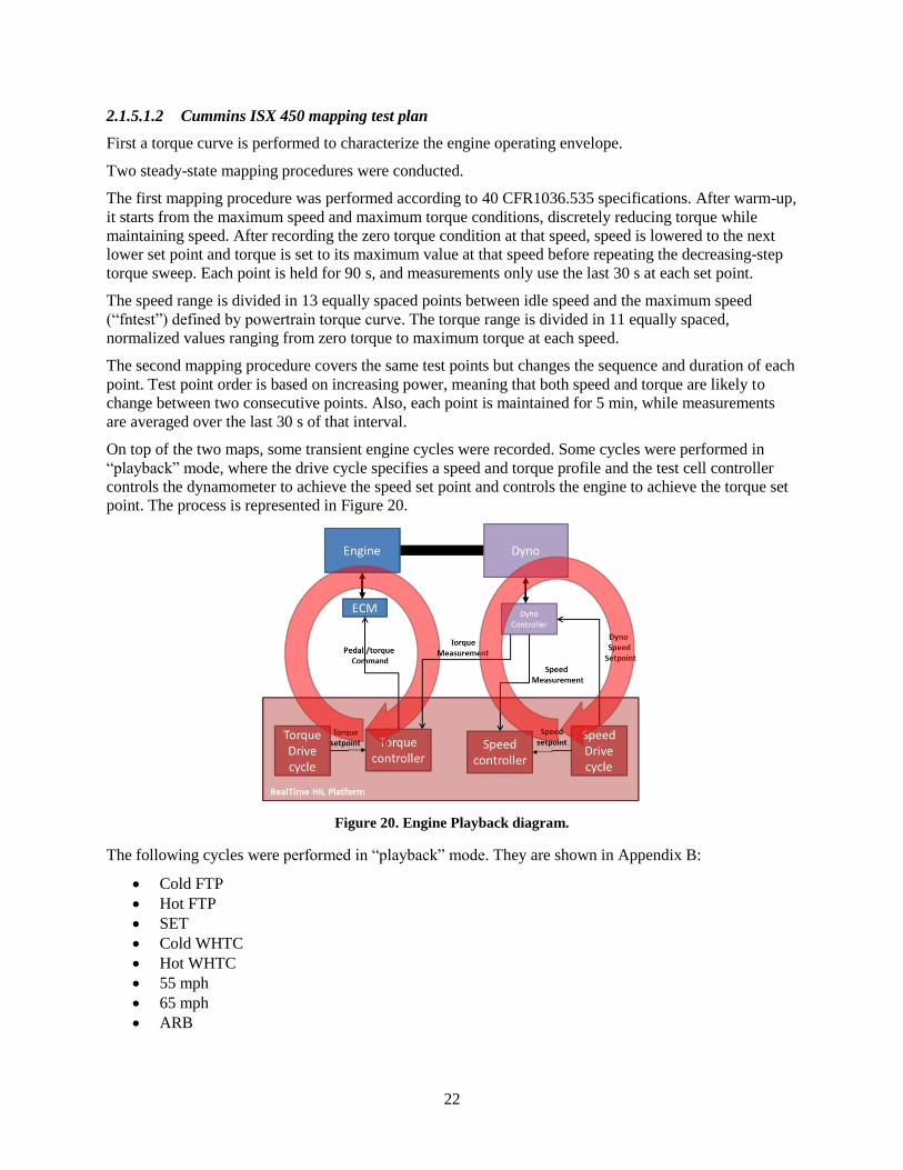
WHVC. .......................................................................................................................................... 10 Figure 8. Original GEM driver (release 2.0.5). ........................................................................................... 10 Figure 9. Modified GEM driver with gain scheduler on proportional term. ............................................... 11 Figure 10. Overall Gem model structure. ................................................................................................... 11 Figure 11. Powertrain interface block. ........................................................................................................ 12 Figure 12. ISX 450 pedal conversion table. ................................................................................................ 12 Figure 13. Effect of grade and mass bypass on transmission work. ........................................................... 14 Figure 14. Effect of grade bypass on AMT shift strategies during ARB cycle. ......................................... 14 Figure 15. Effect of mass bypass on AMT shift strategies during ARB cycle. .......................................... 15 Figure 16. ISX450 engine and UltraShift Plus AMT under test in the Powertrain test cell of
ORNL’s VSI Laboratory. ............................................................................................................... 15 Figure 17. Powertrain-in-the-loop diagram. ............................................................................................... 16 Figure 18. ISX15 450 engine and TC automatic transmission installed in ORNL’s VSI
Laboratory. ..................................................................................................................................... 19 Figure 19. ISX450 engine installed in ORNL’s VSI Laboratory. ............................................................... 21 Figure 20. Engine Playback diagram. ......................................................................................................... 22 Figure 21. Engine-in-the-loop diagram. ...................................................................................................... 23 Figure 22. ISX15 450 engine torque curves. .............................................................................................. 24 Figure 23. Cycle average test points for 55 mph cycle. Effect of minimum engine speed selection. ......... 26 Figure 24. Cycle average test points for 55 mph and 65 mph cruise cycles as well as transient
cycles. test1, 2, and 3 are blue crosses; test 4, 5, and 6 are red x’s; test 8, 9, and 10 are
green stars; test 10 is a pink circle; test 11 is a cyan diamond; and test 12 is square. ................... 26 Figure 25. Cycle average results obtained for ISX 450 engine on transient cycle using fuel
flowmeter measurements. .............................................................................................................. 27 Figure 26. Cycle average results obtained for ISX 450 engine on transient cycle using carbon
balance measurements. .................................................................................................................. 28 Figure 27. ISX15 Engine torque curve for 450 hp cal and 400 hp cal. ....................................................... 28 Figure 28. Cycle average results obtained for ISX 400 engine on transient cycle using fuel
flowmeter measurements. .............................................................................................................. 29 Figure 29. Cycle average results obtained for ISX 400 engine on transient cycle using carbon
balance measurements. .................................................................................................................. 30 Figure 30. ISX15+USP powertrain installed in VSI Laboratory in a single dynamometer
configuration. ................................................................................................................................. 32 Figure 31. Cycle average results obtained for ISX 450 engine on transient cycle using fuel
flowmeter measurements. .............................................................................................................. 33 Figure 32. Interpolation error results for fuel flowmeter measurements on transient cycle. ...................... 34 Figure 33. Interpolation error results for carbon balance measurements on transient cycle. ...................... 34
vi
Figure 34. Interpolation error results for fuel flow measurements on 55 mph cruise cycle. ...................... 35 Figure 35. Interpolation error results for fuel flow measurements on 65 mph cruise cycle. ...................... 35 Figure 36. Interpolation error results for fuel flow measurements for all cycles. ....................................... 35 Figure 37. Interpolation error results for ISX 400 fuel flow measurements on transient cycle. ................. 36 Figure 38. Interpolation error results for ISX 400 fuel flow measurements on 55 mph cruise cycle. ........ 36 Figure 39. Interpolation error results for ISX 400 fuel flow measurements on 65 mph cruise cycle. ........ 36 Figure 40. Interpolation error results for ISX 400 fuel flow measurements for all cycles. ........................ 37 Figure 41. Fuel mass map for ISX 450+USP AMT powertrain using fuel flow measurements on
55 mph cruise cycle. ...................................................................................................................... 38 Figure 42. Interpolation errors on ISX 450+USP AMT powertrain map using fuel flow
measurements on transient cycle.................................................................................................... 39 Figure 43. Interpolation errors on ISX 450+USP AMT powertrain map using fuel flow
measurements on 55 mph cruise. ................................................................................................... 39 Figure 44. Interpolation errors on ISX 450+USP AMT powertrain map using fuel flow
measurements on 65 mph cruise. ................................................................................................... 40 Figure 45. Local interpolation principle on ISX 450+USP AMT powertrain on 65 mph cruise
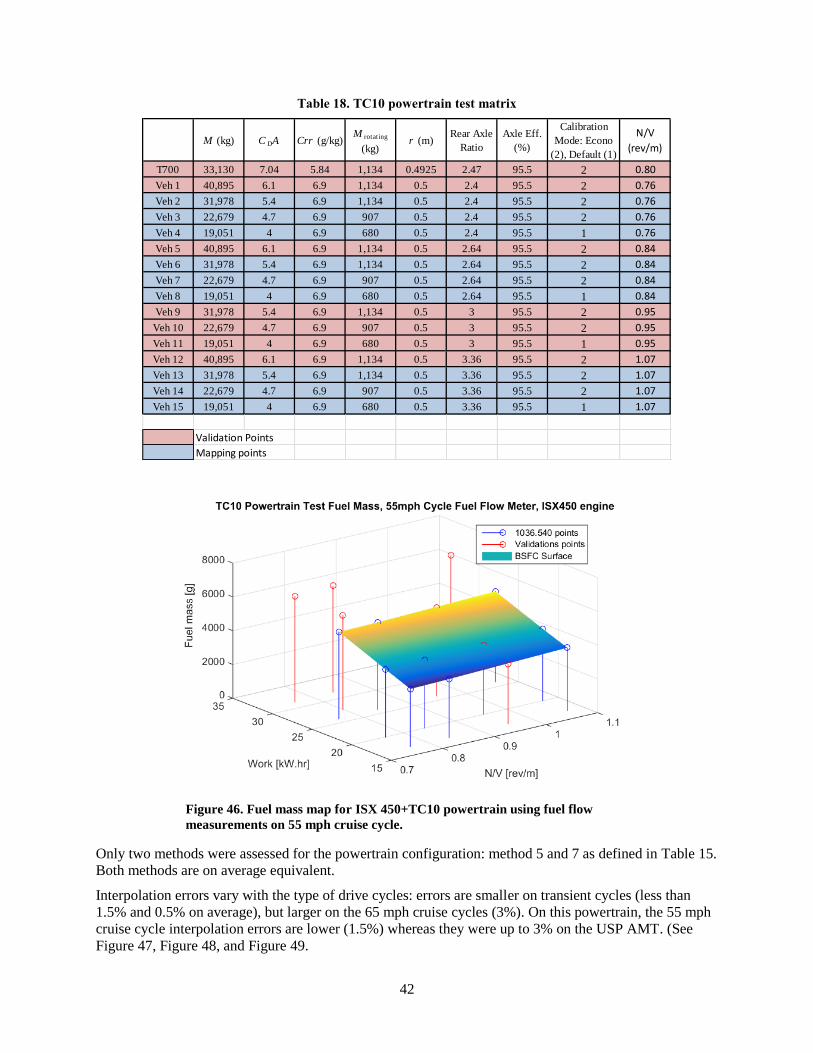
cycle. .............................................................................................................................................. 40 Figure 46. Fuel mass map for ISX 450+TC10 powertrain using fuel flow measurements on 55
mph cruise cycle. ........................................................................................................................... 42 Figure 47. Interpolation errors on ISX 450+ TC10 powertrain map using fuel flow measurements
on transient cycle. .......................................................................................................................... 43 Figure 48. Interpolation errors on ISX 450+ TC10 powertrain map using fuel flow measurements
on 55 mph cruise. ........................................................................................................................... 43 Figure 49. Interpolation errors on ISX 450+TC10 powertrain map using fuel flow measurements
on 65 mph cruise. ........................................................................................................................... 43 Figure 50. Local interpolation principle on ISX 450+TC10 powertrain on 65 mph cruise cycle............... 44 Figure 51. Effect of engine accessory load on match between GEM powertrain map results and
experimental powertrain test results. ............................................................................................. 45 Figure 52. Effect of fueling map behavior during motoring operation on match between GEM
steady-state engine map results and experimental powertrain test results. .................................... 46 Figure 53. Effect of GEM driver on match between GEM powertrain map results and
experimental powertrain test results. ............................................................................................. 47 Figure 54. Effect of powertrain cycle average map size on match between GEM powertrain map
results and experimental powertrain test results. ........................................................................... 48 Figure 55. Comparison of mileage results obtained with GEM powertrain cycle average option,
against powertrain experimental results. ........................................................................................ 49 Figure 56. Comparison of transmission output work results obtained with GEM powertrain cycle
average option, against powertrain experimental results (USP results on left hand side,
TC10 results on right hand side). ................................................................................................... 49 Figure 57. Comparison of fuel flowmeter based fuel mass estimation results obtained with GEM
powertrain cycle average option, against powertrain experimental results (USP results on
left hand side, TC10 results on right hand side). ........................................................................... 50 Figure 58. Comparison of carbon balance based fuel mass estimation results obtained with GEM
powertrain cycle average option, against powertrain experimental results (USP results on
left hand side, TC10 results on right hand side). ........................................................................... 50 Figure 59. Comparison of transmission output work results obtained with GEM steady-state
engine map option, against powertrain experimental results (USP results on left hand
side, TC10 results on right hand side)............................................................................................ 51 Figure 60. Comparison of fuel flowmeter based fuel mass estimation results obtained with GEM
steady-state engine map option, against powertrain experimental results (USP results on
left hand side, TC10 results on right hand side). ........................................................................... 51
vii
Figure 61. Comparison of fuel flowmeter based fuel mass estimation results obtained with GEM
engine cycle average option, against powertrain experimental results (USP results on left
hand side, TC10 results on right hand side). .................................................................................. 52 Figure 62. Comparison of transmission output work results obtained with GEM, against
powertrain experimental results. .................................................................................................... 53 Figure 63. Comparison of fuel mass results obtained with GEM, against powertrain experimental
results (using fuel flow measurements). ........................................................................................ 53 Figure 64. Comparison of fuel mass results obtained with GEM, against powertrain experimental
results (using carbon balance calculations). ................................................................................... 54 Figure 65. Comparison of transmission output work results obtained with GEM steady-state ISX
400 engine map option, against ISX 400 powertrain experimental results (USP results on
left hand side, TC10 results on right hand side). ........................................................................... 55 Figure 66. Comparison of fuel flowmeter based fuel mass estimation results obtained with GEM
(USP results on left hand side, TC10 results on right hand side). ................................................. 55 Figure 67. Comparison of fuel flowmeter based fuel mass estimation results obtained with GEM
ISX 400 engine cycle average option, against ISX 400 powertrain experimental results
(USP results on left hand side, TC10 results on right hand side). ................................................. 56 Figure 68. Comparison of transmission output work results obtained with GEM ISX 400 model,
against ISX 400 powertrain experimental results. ......................................................................... 57 Figure 69. Comparison of fuel mass results obtained with GEM ISX 400 model, against ISX 400
powertrain experimental results. .................................................................................................... 57 Figure 70. Comparison of transmission output work results obtained with GEM ISX 450
powertrain cycle average option, against ISX 400 powertrain experimental results (USP
results on left hand side, TC10 results on right hand side). ........................................................... 58 Figure 71. Comparison of fuel flowmeter based fuel mass estimation results obtained with GEM
ISX 450 powertrain cycle average option, against ISX 400 powertrain experimental
results (USP results on left hand side, TC10 results on right hand side). ...................................... 59 Figure 72. Comparison of transmission output work results obtained with GEM ISX 450 steady-
state engine map option, against ISX 400 powertrain experimental results (USP results on
left hand side, TC10 results on right hand side). ........................................................................... 59 Figure 73. Comparison of fuel flowmeter based fuel mass estimation results obtained with GEM
(USP results on left hand side, TC10 results on right hand side). ................................................. 60 Figure 74. Comparison of fuel flowmeter based fuel mass estimation results obtained with GEM
ISX 450 engine cycle average option, against ISX 400 powertrain experimental results
(USP results on left hand side, TC10 results on right hand side). ................................................. 61 Figure 75. Comparison of transmission output work results obtained with GEM (using ISX 450
engine data), against ISX 400 powertrain experimental results. .................................................... 61 Figure 76. Comparison of fuel mass results obtained with GEM (using ISX 450 engine data),
against ISX 400 powertrain experimental results. ......................................................................... 62 Figure 77. (N/V, Work) vehicle combinations selected for this study. ....................................................... 63 Figure 78. Engine operation during 55 mph and 65 mph cycle for 9 different vehicle
configuration fitted with an automated manual transmission. ....................................................... 63 Figure 79. Engine operation during 55 mph and 65 mph cycle for 9 different vehicle
configuration fitted with an automatic transmission. ..................................................................... 64 Figure 80. Effect of removing 715 rpm, 945 rpm, 1751 rpm and 1982 rpm speed points on CO2
mass estimation when compared with fuel 143-point map. ........................................................... 64 Figure 81. Effect of removing high speed points on CO2 mass estimation when compared with
Figure 82. Effect of removing 10%, 70%, and 90% loads points on CO2 mass estimation when
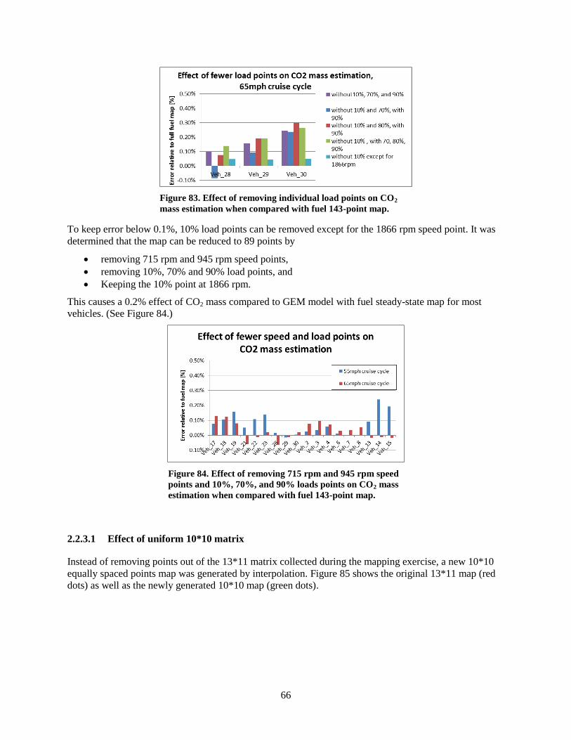
compared with fuel 143-point map. ............................................................................................... 65 Figure 83. Effect of removing individual load points on CO2 mass estimation when compared
with fuel 143-point map. ................................................................................................................ 66 Figure 84. Effect of removing 715 rpm and 945 rpm speed points and 10%, 70%, and 90% loads
points on CO2 mass estimation when compared with fuel 143-point map. ................................... 66 Figure 85. 13*11 fuel map (red cross) and 10*10 fuel map (green x) for ISX 450 engine. ....................... 67 Figure 86. Effect of coarser 10*10 fuel map on CO2 mass estimation when compared with fuel
143-point map. ............................................................................................................................... 67 Figure 87. USP Transmission experimental Powertrain torque curve. ....................................................... 68 Figure 88. USP Transmission experimental and theoretical Powertrain torque curves. ............................. 69 Figure 89. USP Transmission experimental and theoretical powertrain torque curves as well as
powertrain torque during powertrain in the loop wide open acceleration tests. ............................ 69 Figure 90. Engine idle behavior when coupled to an automated manual transmission. ............................. 71 Figure 91. Engine idle behavior when coupled to an automatic transmission. ........................................... 72 Figure 92. TC10 idle fuel flow and torques. ............................................................................................... 73 Figure 93. Powertrain and engine-only idle fuel flows. .............................................................................. 73 Figure 94. Comparison of idle behaviors between experimental results and GEM for automated
manual transmission....................................................................................................................... 74 Figure 95. Comparison of idle behaviors between experimental results and GEM for automatic
transmission. .................................................................................................................................. 74 Figure 96. Distance compensation worst case error as a percentage over all vehicle
configurations. ............................................................................................................................... 75 Figure 97. Distance compensation worst case error as a distance over all vehicle configurations. ............ 75 Figure 98. Powertrain output energy coefficient of variation as a function of vehicle mass. ..................... 76 Figure 99. Example of energy consumption difference due to final drive ratios. ....................................... 76
Run ID Regulatory SubcategoryData Data ConfigurationRatio Data Aerodynamic Drag Area (CdA)Rolling Resistance LevelRolling Resistance LevelRolling Resistance LevelLoaded Tire SizeVehicle Speed LimiterWeight AdjustmentNeutral-Idle
Unique Identifier (e.g. C8_SC_HR) File Name File Name (e.g. 6x4)# File Namem^2 kg/t kg/t kg/t rev/mi MPH or NAlbs Y/N
2018_Engine455_6spdAT_cycle01 C8_SC_HR ISX_ORNL_DEF_C_Bal_Exp_T_Curve.csv Transmissions\EPA_AT_6_HHD_lockup_in_3rd.csv 6x4 3.382 NA 5.4 6.9 6.9 6.9 500 NA 0 Y
2018_Engine455_6spdAT_cycle02 C8_DC_MR ISX_ORNL_DEF_C_Bal_Exp_T_Curve.csv Transmissions\EPA_AT_6_HHD_lockup_in_3rd.csv 6x4 3.382 NA 4.7 6.9 6.9 6.9 500 NA 13275 Y
2018_Engine455_6spdAT_cycle03 C7_DC_MR ISX_ORNL_DEF_C_Bal_Exp_T_Curve.csv Transmissions\EPA_AT_6_HHD_lockup_in_3rd.csv 4x2 3.382 NA 4 6.9 6.9 NA 500 NA 6147 Y
2018_Engine455_6spdAT_cycle04 C8_SC_HR ISX_ORNL_DEF_C_Bal_Exp_T_Curve.csv Transmissions\EPA_AT_6_HHD_lockup_in_3rd.csv 6x4 4.259 NA 5.4 6.9 6.9 6.9 500 NA 0 Y
2018_Engine455_6spdAT_cycle05 C8_DC_MR ISX_ORNL_DEF_C_Bal_Exp_T_Curve.csv Transmissions\EPA_AT_6_HHD_lockup_in_3rd.csv 6x4 4.259 NA 4.7 6.9 6.9 6.9 500 NA 13275 Y
2018_Engine455_6spdAT_cycle06 C7_DC_MR ISX_ORNL_DEF_C_Bal_Exp_T_Curve.csv Transmissions\EPA_AT_6_HHD_lockup_in_3rd.csv 4x2 4.259 NA 4 6.9 6.9 NA 500 NA 6147 Y
2018_Engine455_6spdAT_cycle07 C8_SC_HR ISX_ORNL_DEF_C_Bal_Exp_T_Curve.csv Transmissions\EPA_AT_6_HHD_lockup_in_3rd.csv 6x4 5.45 NA 5.4 6.9 6.9 6.9 500 NA 0 Y
2018_Engine455_6spdAT_cycle08 C8_DC_MR ISX_ORNL_DEF_C_Bal_Exp_T_Curve.csv Transmissions\EPA_AT_6_HHD_lockup_in_3rd.csv 6x4 5.45 NA 4.7 6.9 6.9 6.9 500 NA 13275 Y
2018_Engine455_6spdAT_cycle09 C7_DC_MR ISX_ORNL_DEF_C_Bal_Exp_T_Curve.csv Transmissions\EPA_AT_6_HHD_lockup_in_3rd.csv 4x2 5.45 NA 4 6.9 6.9 NA 500 NA 6147 Y
2018_Engine455_6spdAT_cycle10 C8_DC_MR ISX_ORNL_DEF_C_Bal_Exp_T_Curve.csv Transmissions\EPA_AT_6_HHD_lockup_in_3rd.csv 6x4 3.261 NA 4.7 6.9 6.9 6.9 500 NA 0 Y
2018_Engine455_6spdAT_cycle11 C8_DC_MR ISX_ORNL_DEF_C_Bal_Exp_T_Curve.csv Transmissions\EPA_AT_6_HHD_lockup_in_3rd.csv 6x4 3.805 NA 4.7 6.9 6.9 6.9 500 NA 29762 Y
2018_Engine455_6spdAT_cycle12 C8_SC_HR ISX_ORNL_DEF_C_Bal_Exp_T_Curve.csv Transmissions\EPA_AT_6_HHD_lockup_in_3rd.csv 6x4 4.812 NA 5.4 6.9 6.9 6.9 500 NA 8194 Y
2018_Engine455_10spdAMT_cycle01 C8_SC_HR ISX_ORNL_DEF_C_Bal_Exp_T_Curve.csv Transmissions\EPA_AMT_10_C78_4490_hires.csv 6x4 3.111 NA 5.4 6.9 6.9 6.9 500 NA 0 Y
2018_Engine455_10spdAMT_cycle02 C8_DC_MR ISX_ORNL_DEF_C_Bal_Exp_T_Curve.csv Transmissions\EPA_AMT_10_C78_4490_hires.csv 6x4 3.111 NA 4.7 6.9 6.9 6.9 500 NA 13275 Y
2018_Engine455_10spdAMT_cycle03 C7_DC_MR ISX_ORNL_DEF_C_Bal_Exp_T_Curve.csv Transmissions\EPA_AMT_10_C78_4490_hires.csv 4x2 3.111 NA 4 6.9 6.9 NA 500 NA 6147 Y
2018_Engine455_10spdAMT_cycle04 C8_SC_HR ISX_ORNL_DEF_C_Bal_Exp_T_Curve.csv Transmissions\EPA_AMT_10_C78_4490_hires.csv 6x4 3.918 NA 5.4 6.9 6.9 6.9 500 NA 0 Y
2018_Engine455_10spdAMT_cycle05 C8_DC_MR ISX_ORNL_DEF_C_Bal_Exp_T_Curve.csv Transmissions\EPA_AMT_10_C78_4490_hires.csv 6x4 3.918 NA 4.7 6.9 6.9 6.9 500 NA 13275 Y
2018_Engine455_10spdAMT_cycle06 C7_DC_MR ISX_ORNL_DEF_C_Bal_Exp_T_Curve.csv Transmissions\EPA_AMT_10_C78_4490_hires.csv 4x2 3.918 NA 4 6.9 6.9 NA 500 NA 6147 Y
2018_Engine455_10spdAMT_cycle07 C8_SC_HR ISX_ORNL_DEF_C_Bal_Exp_T_Curve.csv Transmissions\EPA_AMT_10_C78_4490_hires.csv 6x4 5.014 NA 5.4 6.9 6.9 6.9 500 NA 0 Y
2018_Engine455_10spdAMT_cycle08 C8_DC_MR ISX_ORNL_DEF_C_Bal_Exp_T_Curve.csv Transmissions\EPA_AMT_10_C78_4490_hires.csv 6x4 5.014 NA 4.7 6.9 6.9 6.9 500 NA 13275 Y
2018_Engine455_10spdAMT_cycle09 C7_DC_MR ISX_ORNL_DEF_C_Bal_Exp_T_Curve.csv Transmissions\EPA_AMT_10_C78_4490_hires.csv 4x2 5.014 NA 4 6.9 6.9 NA 500 NA 6147 Y
2018_Engine455_10spdAMT_cycle10 C8_DC_MR ISX_ORNL_DEF_C_Bal_Exp_T_Curve.csv Transmissions\EPA_AMT_10_C78_4490_hires.csv 6x4 3 NA 4.7 6.9 6.9 6.9 500 NA 0 Y
2018_Engine455_10spdAMT_cycle11 C8_DC_MR ISX_ORNL_DEF_C_Bal_Exp_T_Curve.csv Transmissions\EPA_AMT_10_C78_4490_hires.csv 6x4 3.501 NA 4.7 6.9 6.9 6.9 500 NA 29762 Y
2018_Engine455_10spdAMT_cycle12 C8_SC_HR ISX_ORNL_DEF_C_Bal_Exp_T_Curve.csv Transmissions\EPA_AMT_10_C78_4490_hires.csv 6x4 4.427 NA 5.4 6.9 6.9 6.9 500 NA 8194 Y
28
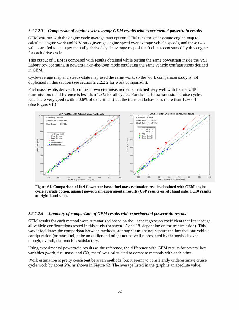
Figure 26. Cycle average results obtained for ISX 450 engine
on transient cycle using carbon balance measurements.
Run ID Regulatory Subcategory Data Data ConfigurationRatio Data Aerodynamic Drag Area (CdA)Rolling Resistance LevelRolling Resistance LevelRolling Resistance LevelLoaded Tire SizeVehicle Speed LimiterWeight AdjustmentNeutral-Idle
Unique Identifier (e.g. C8_SC_HR) File Name File Name (e.g. 6x4) # File Name m^2 kg/t kg/t kg/t rev/mi MPH or NAlbs Y/N
2018_Engine400_6spdAT_cycle01 C8_SC_HR ISX400_ORNL_DEF_C_Bal_Exp_T_Curve.csv Transmissions\EPA_AT_6_HHD_lockup_in_3rd.csv 6x4 3.382 NA 5.4 6.9 6.9 6.9 500 NA 0 Y
2018_Engine400_6spdAT_cycle02 C8_DC_MR ISX400_ORNL_DEF_C_Bal_Exp_T_Curve.csv Transmissions\EPA_AT_6_HHD_lockup_in_3rd.csv 6x4 3.382 NA 4.7 6.9 6.9 6.9 500 NA 13275 Y
2018_Engine400_6spdAT_cycle03 C7_DC_MR ISX400_ORNL_DEF_C_Bal_Exp_T_Curve.csv Transmissions\EPA_AT_6_HHD_lockup_in_3rd.csv 4x2 3.382 NA 4 6.9 6.9 NA 500 NA 6147 Y
2018_Engine400_6spdAT_cycle04 C8_SC_HR ISX400_ORNL_DEF_C_Bal_Exp_T_Curve.csv Transmissions\EPA_AT_6_HHD_lockup_in_3rd.csv 6x4 4.259 NA 5.4 6.9 6.9 6.9 500 NA 0 Y
2018_Engine400_6spdAT_cycle05 C8_DC_MR ISX400_ORNL_DEF_C_Bal_Exp_T_Curve.csv Transmissions\EPA_AT_6_HHD_lockup_in_3rd.csv 6x4 4.259 NA 4.7 6.9 6.9 6.9 500 NA 13275 Y
2018_Engine400_6spdAT_cycle06 C7_DC_MR ISX400_ORNL_DEF_C_Bal_Exp_T_Curve.csv Transmissions\EPA_AT_6_HHD_lockup_in_3rd.csv 4x2 4.259 NA 4 6.9 6.9 NA 500 NA 6147 Y
2018_Engine400_6spdAT_cycle07 C8_SC_HR ISX400_ORNL_DEF_C_Bal_Exp_T_Curve.csv Transmissions\EPA_AT_6_HHD_lockup_in_3rd.csv 6x4 5.45 NA 5.4 6.9 6.9 6.9 500 NA 0 Y
2018_Engine400_6spdAT_cycle08 C8_DC_MR ISX400_ORNL_DEF_C_Bal_Exp_T_Curve.csv Transmissions\EPA_AT_6_HHD_lockup_in_3rd.csv 6x4 5.45 NA 4.7 6.9 6.9 6.9 500 NA 13275 Y
2018_Engine400_6spdAT_cycle09 C7_DC_MR ISX400_ORNL_DEF_C_Bal_Exp_T_Curve.csv Transmissions\EPA_AT_6_HHD_lockup_in_3rd.csv 4x2 5.45 NA 4 6.9 6.9 NA 500 NA 6147 Y
2018_Engine400_6spdAT_cycle10 C8_DC_MR ISX400_ORNL_DEF_C_Bal_Exp_T_Curve.csv Transmissions\EPA_AT_6_HHD_lockup_in_3rd.csv 6x4 3.261 NA 4.7 6.9 6.9 6.9 500 NA 0 Y
2018_Engine400_6spdAT_cycle11 C8_DC_MR ISX400_ORNL_DEF_C_Bal_Exp_T_Curve.csv Transmissions\EPA_AT_6_HHD_lockup_in_3rd.csv 6x4 3.805 NA 4.7 6.9 6.9 6.9 500 NA 29762 Y
2018_Engine400_6spdAT_cycle12 C8_SC_HR ISX400_ORNL_DEF_C_Bal_Exp_T_Curve.csv Transmissions\EPA_AT_6_HHD_lockup_in_3rd.csv 6x4 4.812 NA 5.4 6.9 6.9 6.9 500 NA 8194 Y
2018_Engine400_10spdAMT_cycle01 C8_SC_HR ISX400_ORNL_DEF_C_Bal_Exp_T_Curve.csv Transmissions\EPA_AMT_10_C78_4490_hires.csv 6x4 3.111 NA 5.4 6.9 6.9 6.9 500 NA 0 Y
2018_Engine400_10spdAMT_cycle02 C8_DC_MR ISX400_ORNL_DEF_C_Bal_Exp_T_Curve.csv Transmissions\EPA_AMT_10_C78_4490_hires.csv 6x4 3.111 NA 4.7 6.9 6.9 6.9 500 NA 13275 Y
2018_Engine400_10spdAMT_cycle03 C7_DC_MR ISX400_ORNL_DEF_C_Bal_Exp_T_Curve.csv Transmissions\EPA_AMT_10_C78_4490_hires.csv 4x2 3.111 NA 4 6.9 6.9 NA 500 NA 6147 Y
2018_Engine400_10spdAMT_cycle04 C8_SC_HR ISX400_ORNL_DEF_C_Bal_Exp_T_Curve.csv Transmissions\EPA_AMT_10_C78_4490_hires.csv 6x4 3.918 NA 5.4 6.9 6.9 6.9 500 NA 0 Y
2018_Engine400_10spdAMT_cycle05 C8_DC_MR ISX400_ORNL_DEF_C_Bal_Exp_T_Curve.csv Transmissions\EPA_AMT_10_C78_4490_hires.csv 6x4 3.918 NA 4.7 6.9 6.9 6.9 500 NA 13275 Y
2018_Engine400_10spdAMT_cycle06 C7_DC_MR ISX400_ORNL_DEF_C_Bal_Exp_T_Curve.csv Transmissions\EPA_AMT_10_C78_4490_hires.csv 4x2 3.918 NA 4 6.9 6.9 NA 500 NA 6147 Y
2018_Engine400_10spdAMT_cycle07 C8_SC_HR ISX400_ORNL_DEF_C_Bal_Exp_T_Curve.csv Transmissions\EPA_AMT_10_C78_4490_hires.csv 6x4 5.014 NA 5.4 6.9 6.9 6.9 500 NA 0 Y
2018_Engine400_10spdAMT_cycle08 C8_DC_MR ISX400_ORNL_DEF_C_Bal_Exp_T_Curve.csv Transmissions\EPA_AMT_10_C78_4490_hires.csv 6x4 5.014 NA 4.7 6.9 6.9 6.9 500 NA 13275 Y
2018_Engine400_10spdAMT_cycle09 C7_DC_MR ISX400_ORNL_DEF_C_Bal_Exp_T_Curve.csv Transmissions\EPA_AMT_10_C78_4490_hires.csv 4x2 5.014 NA 4 6.9 6.9 NA 500 NA 6147 Y
2018_Engine400_10spdAMT_cycle10 C8_DC_MR ISX400_ORNL_DEF_C_Bal_Exp_T_Curve.csv Transmissions\EPA_AMT_10_C78_4490_hires.csv 6x4 3 NA 4.7 6.9 6.9 6.9 500 NA 0 Y
2018_Engine400_10spdAMT_cycle11 C8_DC_MR ISX400_ORNL_DEF_C_Bal_Exp_T_Curve.csv Transmissions\EPA_AMT_10_C78_4490_hires.csv 6x4 3.501 NA 4.7 6.9 6.9 6.9 500 NA 29762 Y
2018_Engine400_10spdAMT_cycle12 C8_SC_HR ISX400_ORNL_DEF_C_Bal_Exp_T_Curve.csv Transmissions\EPA_AMT_10_C78_4490_hires.csv 6x4 4.427 NA 5.4 6.9 6.9 6.9 500 NA 8194 Y
30
Figure 29. Cycle average results obtained for ISX 400 engine
on transient cycle using carbon balance measurements.
2.1.6 Evaluate Advanced HD Engine and Powertrain Technologies
This task was contingent upon available funds and performance on previous tasks. It was intended to
evaluate advanced HD engines and powertrain technologies and the test procedures required to quantify
their performance.
The details of this task have not been specified by the EPA yet, and no work has been performed.
2.1.7 Road Grade Cycles
2.1.7.1.1 Road grade cycle (ISX 450 engine) mapping test plan
EPA provided four grade profiles to be run in both forward and reverse directions at 55 mph and 65 mph
for a total of 10 different drive cycles (the grade profiles are shown in Appendix A):
Grade Profile A, Test Speed: 55 mph, Trace Direction: forward
Grade Profile A, Test Speed: 55 mph, Trace Direction: reverse
Grade Profile A, Test Speed: 65 mph, Trace Direction: forward
Grade Profile A, Test Speed: 65 mph, Trace Direction: reverse
Grade Profile B, Test Speed: 55 mph, Trace Direction: forward
Grade Profile B, Test Speed: 55 mph, Trace Direction: reverse
Grade Profile C, Test Speed: 65 mph, Trace Direction: forward
Grade Profile C, Test Speed: 65 mph, Trace Direction: reverse
Grade Profile D, Test Speed: 55 mph, (symmetrical)
Grade Profile D, Test Speed: 65 mph, (symmetrical)
These drive cycles are applied to two powertrains:
Cummins ISX15 (450 hp cal) engine coupled to Allison TC10 automatic transmission
Cummins ISX15 (450 hp cal) engine coupled to Eaton UltraShift Plus AMT
The VSI Laboratory was operated in powertrain-in-the-loop mode with the “1037-equation” model.
The vehicle configurations performed with the TC10 transmission are listed in Table 11.
31
Table 11. Vehicle configurations performed with the TC10 transmission
M (kg) CDA Crr (g/kg) Mrotating
(kg) r (m)
Rear
Axle
Ratio
Axle Eff.
(%)
Calibration Mode:
Econo (2), Default
(1)
Veh 2
31,978 5.4 6.9 1,134 0.5
2.4
95.5 2 Veh 6 2.64
Veh 13 3.36
The vehicle configurations performed with the UltraShift transmission are listed in Table 12.
Table 12. Vehicle configurations performed with the UltraShift transmission
M (kg) CDA Crr (g/kg) Mrotating
(kg) r (m)
Rear
Axle
Ratio
Axle Eff.
(%)
Veh 13
31,978 5.4 6.9 1,134 0.5
3.36
95.5 Veh 17 2.81
Veh 28 4.65
Because the TC10 automatic transmission has two modes (economy and performance), this transmission
was tested on two more vehicles (#2 and #13) with a subset of four cycles:
Grade Profile B , 55 mph, forward
Grade Profile C, 65 mph, forward
Grade Profile D, 55 mph
Grade Profile D, 65 mph
All operations procedures were also summarized in the Quality Assurance Project Plan
(EPA_GHG2_QAPP_draft10.docx).
2.1.7.1.2 Road grade cycle (ISX 450 engine) mapping test results
Table 13 and Table 14 show respectively the TC10 and UltraShift test matrixes; dates are those on which
tests were performed.
Table 13. TC10 powertrain test tracker of grade cycle test matrix
Table 14. USP powertrain test tracker of grade cycle test matrix
55mph Profile B Fwd 55mph Profile B Rvrs 55mph Profile A Fwd 55mph Profile A Rvrs 65mph Profile A Fwd 65mph Profile A Rvrs 65mph Profile C Fwd 65mph Profile C Rvrs 55mph Profile D 65mph Profile D
55mph Profile B Fwd 65mph Profile C Fwd 55mph Profile D 65mph Profile D
Veh 2 8/13/2015 8/13/2015 8/13/2015 8/13/2015
Veh 13 8/11/2015 8/11/2015 8/13/2015 8/13/2015
55mph Profile B Fwd 55mph Profile B Rvrs 55mph Profile A Fwd 55mph Profile A Rvrs 65mph Profile A Fwd 65mph Profile A Rvrs 65mph Profile C Fwd 65mph Profile C Rvrs 55mph Profile D 65mph Profile D