38
Natural Sciences Tripos Part II MA TERIALS SCIENCE Practicals and Materials Examination Series 2011-12 II
| Date post: | 06-Apr-2018 |
| Category: |
Documents |
| Upload: | qaiser-ali |
| View: | 219 times |
| Download: | 0 times |

8/3/2019 Practical Booklet
http://slidepdf.com/reader/full/practical-booklet 1/38

8/3/2019 Practical Booklet
http://slidepdf.com/reader/full/practical-booklet 2/38
1
Practicals and materials examination series
The experimental work includes 5 practicals and 4 materials examination series, a subset of
which is carried out in the Michaelmas term.
Practicals should be carried out in groups of approximately 4. Each group will have a
timetable, for practicals and materials examination series, allocated at the beginning of the
Michaelmas term. All work should be recorded in the laboratory note-book distributed. Books
will be marked following completion of the exercise in order to ensure that immediate
comments on work are obtained. You will select one of the practicals to write up during the
Lent Term.
Practicals take place on Fridays (11 am - 5 pm) and Monday mornings (10 am - 1 pm). The
Materials Examination series can be done at any time during the appropriate week, as
availability of equipment (i.e. the SEM) allows. These should take just a few hours tocomplete.
Practicals
P1: Thermal distortion in composites TWC
P2: Atomic force microscopy RAO
P3: Polymer crystallization REC
P4: Casting ERWP5: Oxidation of titanium JAL
Materials Examination series
M1: Woods ALG
M2: Biomedical materials SMB
M3: Brazing and welding PEJR
M4: Fracture Mechanisms CR
Laboratory notebooks should be handed into the box in Lab 301 by 1pm on the Tuesday followingeach practical. They will be marked by the demonstrators and returned to you in time for your next
practical.
Contact Professor Best immediately if you foresee any problems in meeting the 1pm deadline,
due to equipment failure etc.

8/3/2019 Practical Booklet
http://slidepdf.com/reader/full/practical-booklet 3/38
2
Keeping notes and writing up experimental work
Time takenPracticals should take you less than 8 hours to complete in full. This includes the time to actually
carry out the processing and measurements, to record your results and to carry out the analysis as
you go along. The Materials Examination series should take less time – a couple of hours of
making observations and a couple more to understand your observations and describe them in more
detail.
Keeping a lab book
In any experiment, you should keep notes about what you are doing as you go along. This includes
any special details of experimental procedures and equipment used. It also includes measurementsmade, sketches, photographs, odd observations and so forth. All of these should be noted. Says
what things are. Often one can make measurements at a range of, say, temperatures. Do not rely on
your memory. You should include comments on your sketches, as well as magnifications.
If you are looking at, say, a microstructure, make a brief description, trying to summarise what you
see at that moment as the essential points. As you look at it more, your view may begin to change
and you may have to go back.
You should keep all your notes in a notebook. If you do absolutely have to take some notes on a
scrap of paper, stick the scrap of paper in the book to avoid transcription errors. For the same
reason, do not take notes and then copy them into a book later on grounds of ‘neatness’. Accuracy
is more important here than a clean page. However life will be much easier if you try and keep
things as clear as you can.
It is in the nature of real things that they do not always go quite as planned. Try to explain why
they might have arisen, even better what you did to overcome them, or, if that is not possible, how
they might be overcome. If there are problems with experimental equipment, be sure to report this
at the time and on the feedback form.
For the purposes of assessment of each practical, you should also carry out some analysis of your
results (for example, plot graphs to show experimental data, calculate parameters etc.). All this
should be done in the lab book and as far as possible should be done as the practical proceeds. If
you attempt to “finish” the experiment and then do the analysis, you will commonly find that there
are a few extra things that you wish that you’d measured (and in the worst-case scenario, you may
find that all your experimental data are useless because all your careful measurements are on a
sample that someone dropped on the floor). In producing graphs, most of the advice given in
section 3 below (referring to preparing formal reports) is relevant.
Finally, attempt to draw some (brief) conclusions based on what you have observed. This is not
meant to be a full write up, so you are not expected to trawl through text-books in order to explain
the gory details of the theory and figure out what the measurements “should” show if you’d had
several months to refine the experiment and make thousands of measurements.
If you tried something that did not work, say so. For instance, a particular etch may not have been
useful. Record it in your notes and then make a brief note in your conclusions.
There can be no guidelines as to “how much” you should write. The number of pages filled in your

8/3/2019 Practical Booklet
http://slidepdf.com/reader/full/practical-booklet 4/38
3
book will depend on how many numbers you need to write down, how many graphs you plot and
how many images and sketches you generate. The actual written explanations should be as concise
as possible. Just a page or two of writing is probably about right.
Because you are doing things as you proceed, hand-written work is generally preferred for things in
your lab book (except of course for any things which are computer-generated such as plots and
photographs). If you think your hand-writing is illegible, then a small amount of type-written text
is OK as long as it is properly stuck into your lab book.
Carrying out a materials examination series
The aim of these series is to become familiar with certain types of structure. The approach here is
essentially the same. Your lab book should consist of the sketches or photographs of the structures
you have examined, together with a description of the individual structures one by one. Again your
views as to the important features may change and you may have to go back.
Writing a formal report on a practical
One of the practicals will be written up more formally during the Lent Term. The aim again is to
record and rationalise observations, measurements and calculations that were made so that it may
be understood by another scientist. You should aim to make the write-up as concise as you possibly
can. There is no extra credit for extra weight. The length of the write-up can vary, but you might
think of 3000 words as being a very rough rule-of thumb.
The formal report should generally be computer word-processed, though handwritten pencil
sketches and annotations are fine.
The written formal report should probably follow the conventions:
1. Introduction or Abstract: This describes the problem and the aim of the experiment and
may also summarise the main conclusion.
2. Experimental: This gives the basic approach, and describes the methods, techniques and
equipment in suitable detail (without simply repeating what is already in the practical
booklet). This allows the reader to see clearly (and in one place) exactly what methods
were used.
3. Results: These should be described in a way that a reader can most easily comprehend, i.e.by graphs and suitable figures. For graphs, say what variables are being plotted. Figures
should have captions and you should be able to see the features you are showing. Sad
though it may sound, a caption which captures the essential details of the point you are
trying to make with the figure can be very effective. Captions such as “Arrhenius plot” are
useless. Graphs should be drawn properly on graph paper or electronically. A little scribbly
biro sketch, claiming that this is what the graph might look like if anybody could be
bothered to draw it out is no good. Figures should not just be space-fillers. Don’t put them
in because you think a figure, perhaps in-blue, might look rather natty in the left-hand
corner. All figures should be properly referred to in the text and they should show clearly
what is claimed.

8/3/2019 Practical Booklet
http://slidepdf.com/reader/full/practical-booklet 5/38
4
4. Discussion: This is the point where you should try and rationalise what you have seen or
calculated. It is where you justify these ideas. You can also discuss your results in the
context of other literature. This is very open-ended. Sometimes there is a reference or two
at the end of the practical – these can help you understand what is going on and put your
results into context. Often one sees papers where the results and discussion are mixedtogether. There is nothing wrong with this, provided it makes the write-up clearer to the
reader.
5. Conclusions: These should be drawn from the work you actually did, not what you think it
was about. The ideas should have been discussed above and not suddenly appear for the
first time. They should be short and concise.
List of Supervisors and Demonstrators
Practical Subject Supervisor Demonstrator Email
M1 Woods AL Greer (alg13) FA Clarke fac23
M2 Biomedical Materials SM Best (smb51) JH Gwynne jhg27
K-A Kwon kak31
WR Skelton-Hough wrh23
M3 Brazing and Welding PEJ Rivera (pejr2) PFF Walker pffw2
M4 Fracture CMF Rae (cr18) S Birosca sb833
P1 Composites TW Clyne (twc10) SK Lam skl38
EK Oberg eko23
VMT Su vmts2
P2 AFM RA Oliver (rao28) S Bennett sb534
T Zhu tz234
P3 Polymers RE Cameron (rec11) D Ege de258
RJ Friederichs rjf52
KM Pawelec kmp42
P4 Casting HJ Stone (hjs1002) L Mirelman lm351
M Shinozaki ms660
P5 Oxidation of Titanium C Schwandt (cs254) C Schwandt cs254
8/3/2019 Practical Booklet
http://slidepdf.com/reader/full/practical-booklet 6/38
5
P1: Thermal distortion in composites
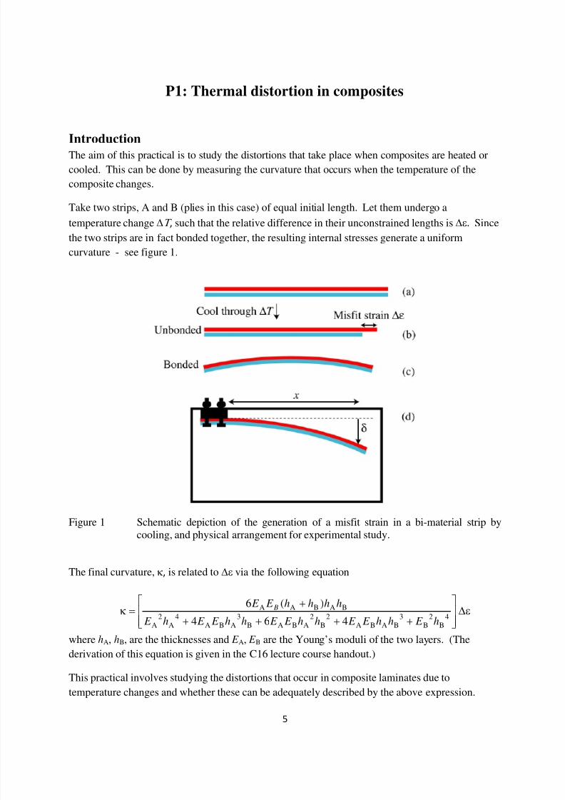
IntroductionThe aim of this practical is to study the distortions that take place when composites are heated or
cooled. This can be done by measuring the curvature that occurs when the temperature of the
composite changes.
Take two strips, A and B (plies in this case) of equal initial length. Let them undergo a
temperature change ∆Τ , such that the relative difference in their unconstrained lengths is ∆ε. Since
the two strips are in fact bonded together, the resulting internal stresses generate a uniform
curvature - see figure 1.
Figure 1 Schematic depiction of the generation of a misfit strain in a bi-material strip by
cooling, and physical arrangement for experimental study.
The final curvature, κ, is related to ∆ε via the following equation
ε∆
++++
+=κ
464
)(64
B
2
B
3
BABA
2
B
2
ABAB
3
ABA
4
A
2
A
BABAA
h E hh E E hh E E hh E E h E
hhhh E E B
where hA, hB, are the thicknesses and E A, E B are the Young’s moduli of the two layers. (The
derivation of this equation is given in the C16 lecture course handout.)
This practical involves studying the distortions that occur in composite laminates due to
temperature changes and whether these can be adequately described by the above expression.

8/3/2019 Practical Booklet
http://slidepdf.com/reader/full/practical-booklet 7/38
6
Before starting
• What is the physical meaning of ∆ε here (see figure 1)? Under what conditions is this not
the case?
• What measurements are required to obtain ∆ε from κ?• For a given pair of materials, is the curvature dependent just on the thickness ratio, or does it
also vary with the absolute values of the thickness?
Basic experimental work
Two materials are available:
• long AS carbon fibres (high strength) in a matrix of Nylon 6 (a thermoplastic polymer)
• long Kevlar 49 fibres, also in Nylon 6
For each type of composite, note the differences in the out-of-plane distortions created during
cooling for non-symmetrical and symmetrical cross-ply laminates.
Analysis of results
Measure the magnitude of the curvature exhibited by the two non-symmetrical laminates and hence
obtain an estimate of ∆ε. Explain why the two lay-ups and two materials behave differently.
Relate this quantitatively to the properties of the composites. Is this what you would expect?
Comment on any discrepancies.
Experimental procedures
Making unidirectional and cross-ply composites
The material is provided initially in the form of a pre-preg tape, composed of mingled strands of
fibre tows and polymeric material. The pre-preg tape is first cut into suitable lengths, which are
stacked in a prescribed sequence. Three types of stacking can be studied:
• unidirectional (fibre directions of each layer all parallel),
• simple cross-ply (two unidirectional stacks with fibre directions at 90° to each other)
• a symmetrical cross-ply arrangement (in which the stacking sequence has a mirror plane in
the centre).
The specimens are all to be composed of 12 plies, giving a total thickness of about 2 mm. The
laminates are all about 150 mm square. The laminates are produced by a simple hot pressing
operation. A set of three laminates of a given composite can be made in a single operation, by
alternately stacking aluminium plates and ply stacks. Release agent is sprayed onto the metal
plates before assembling the stack. Pressing is carried out at a temperature of 230-240 °C, for a
period of 20-30 minutes. This should be sufficient to melt the matrix and generate enough flow to
eliminate internal porosity. A pressure of 500 psi is maintained on the ram during pressing.

8/3/2019 Practical Booklet
http://slidepdf.com/reader/full/practical-booklet 8/38
7
After inspection of both cross-ply laminates, a further strip, about 140 mm by 20 mm, is cut from
each of the simple cross-ply samples, with its length parallel to one of the two fibre directions.
These are to be used for thermal contraction measurements.
Two strips, about 120 mm long by 20 mm wide, are to be cut from each of the unidirectionalcomposites (Kevlar and carbon), one with the length parallel to the fibre direction and one
transverse to it. These will be used for stiffness measurement.
Measurement of anisotropy of thermal contraction
After drilling suitable holes through the cross-ply laminate, fix it securely in the tray, using the
bolts and wing nuts provided, locating the spacer block between the side of the tray and the strip, as
shown in figure 1. Ensure that the side with the smaller expansion coefficient α (the ply with the
fibres parallel to the length) is closest to the wall of the tray, so that laminate will curve away from
the nearest wall when cooled.
Carefully pour liquid nitrogen into the tray, so that the laminate is partially immersed. (Gloves
should be worn for this operation.) When thermal equilibrium is reached, measure the lateral
displacement, using the scale provided on the lid. The resulting curvature, κ, (reciprocal of the
radius of curvature) is related to the displacement, δ, and the distance, x , along the strip at which
the displacement is being measured, by
κ =
2sin tan−1 δ
x
x2 + δ
2( )
The derivation of this relationship is shown in figure 2. The specimen may have an initial
curvature at room temperature. The change induced by cooling to liquid nitrogen temperature is
required.
Figure 2 The relationship between the curvature, κ, and the displacement, δ.

8/3/2019 Practical Booklet
http://slidepdf.com/reader/full/practical-booklet 9/38
8
Measurement of Young Modulus
The Young’s moduli in axial and transverse directions are measured by symmetrical 3-point bend
testing. The following equation relates the measured deflection of the centre of the beam, d, the
length of the beam, L, and the applied load, P
δ =1
48
PL3
EI
where E is the axial Young’s modulus of the beam and I is its second moment of area. For a
prismatic beam with a rectangular section (depth h and width w), the value of I is given by
I =w h3
12
ReferencesIt may prove useful to consult various sources about different aspects of fibres, composites and
testing procedures, but the reference below will provide much of the general background required.
1. D. Hull & T.W. Clyne, Introduction to Composite Materials, 2nd edn., Cambridge
University Press, Cambridge, 1996.

8/3/2019 Practical Booklet
http://slidepdf.com/reader/full/practical-booklet 10/38
9
P2: Atomic Force Microscopy
IntroductionAtomic Force Microscopy (AFM) is a powerful tool for imaging surface morphology. It can be
used for high resolution imaging of a wide range of samples, irrespective of their conductivity, and
is thus an increasingly useful tool in the rapidly expanding field of nanotechnology. AFM is used
in a wide range of applications from optimisation of semiconductor devices to nanoscale studies of
the surfaces of living cells. It has even been used on the surface of Mars to investigate the structure
of Martian dirt!
(See http://www.famars.unibas.ch/index.htm for more information on the Mars project.)
In the first half of this practical you will get the opportunity to use a Nanosurf easyScan 2 AFMbased in the class lab to image a CD, in order to familiarise yourself with the operation of the
instrument and the analysis of the resulting images.
In the second half of the practical you will be able to put your new found skills to use whilst
investigating the self-assembly of colloidal crystals during solvent evaporation.
Aims of practical
• Learn the basics of operating the Nanosurf easyScan 2 AFM
• Understand the principals of AFM operation and methods for optimising AFM images
• Use the AFM to make measurements of micro- and nanoscale features. • Observe the formation of self-assembled colloidal crystals, and defects within the self-
assembled crystals.
• Start to understand the factors which influence the self-assembly of colloidal crystals.
Before Starting
• What limits the resolution of a perfect optical microscope?
• The vertical resolution of the AFM is excellent. High-quality AFMs are capable of atomic-
scale resolution (~0.3A) in the vertical direction. What limits its resolution in the
horizontal direction?
Experimental procedure
1. Sample preparation
a. The CD Compact discs are 1.2 mm thick and comprised almost entirely of polycarbonate.
This polycarbonate layer contains bumps, which encode the data. No data has been written on the
CD provided. For this type of CD, a laser would be used to write the data creating lumps on the
raised tracks. (See e.g. http://www.chem.uga.edu/mlay/nanogallery.htm). This is then covered by a
reflective layer, to reflect the laser back to the detector, and a thin lacquer, which protects the CD.

8/3/2019 Practical Booklet
http://slidepdf.com/reader/full/practical-booklet 11/38
10
You are provided with a delaminated CD – one with the lacquer removed, so you will be able to
image the tracks on the CD. No further sample preparation is required for the CD.
b. Colloidal crystals The colloidal particles are provided as a suspension consisting of 0.46 µm
polystyrene beads dispersed in water (from Sigma-Aldrich, catalogue no. LB5). The suspension is10% polystyrene by weight. You will drop cast the suspension onto a glass slide and leave it to
dry. This should be done before you start imaging the CD, so that the sample can dry whilst you
are examining the CD. First, glass slides should be cut up into pieces which can easily fit on the
AFM stage (i.e cut approximately in half). To do this wear goggles and gloves and be careful of
the sharp edges. Take 2 clean slides. With the scribe provided and using one of the slides like a
ruler, scratch a straight line across the slide about halfway along. Sandwich the scratched slide
between two other slides with the edges of the sandwiching slides lined up with the scratch. If you
now press on the free end of the slide, it should break along the scratch. Next, using a disposable
pipette, drip two small (ideally about 5 mm diameter) drops of the colloidal suspension onto your
half slide. During the first 10 to 15 minutes of drying, watch the drops under an optical
microscope. (Take care to keep the slide horizontal as you transfer it to the optical microscope).
Where in the drop does drying take place first? Complete drying of the drop will take up to 2
hours, so after making some initial observations, leave the half slide to finish drying and go on with
the CD measurements.
2. Imaging the CD
a. AFM operation In AFM, a sharp tip at the end of a small, flexible cantilever is scanned over a
sample surface and the deflection of the cantilever is used to measure the varaitions in the surface's
height. You will be using the AFM in dynamic force mode (sometimes called tapping mode). In
this mode, we use an oscillating cantilever. As the cantilever gets closer to the surface, for a given
drive oscillation, the amplitude of vibration of the cantilever will decrease. Hence, the cantilever’s
oscillation amplitude can be used as a measure of tip-surface distance. As the cantilever is scanned
over the surface, a feedback loop is used to maintain a constant oscillation amplitude (known as the
set-point amplitude). The microscope is calibrated so that the voltages applied to move the scanner
over the surface to maintain the set-point amplitude (and hence to maintain a fixed tip-sample
distance) can be converted into the changes in the height of the sample which necessitated the
scanner movements.
To image the CD, place the CD on the anti-vibration table. You may lift the AFM off its stage and
place it directly on the CD. Ask your demonstrator to help you set up the AFM. Information is
also given in the Nanosurf Easyscan 2 AFM Operating Instructions. The stages of the setup whichyou will need to perform will be:
• Starting up the vibration isolation table.
• Starting up the software
• Manual coarse approach of the tip to the surface (see Operating Instructions, page 40)
• Manual approach using the approach stage (see Operating Instructions, page 40)
• Performing a frequency sweep to find the cantilever’s natural frequency of oscillation (seeOperating Instructions, page 42)
• Setting initial parameters (see Operating Instructions, page 43)
• Automatic final approach (see Operating Instructions, page 41-43)
This sequence will bring the tip into close proximity with the surface (hopefully without damaging
it) and allow you to start imaging. You will need then to optimise the operation of the feedback

8/3/2019 Practical Booklet
http://slidepdf.com/reader/full/practical-booklet 12/38
11
circuit which attempts to maintain the fixed tip-sample distance. Again, your demonstrator should
help you with this the first time you try it. The basic idea is that the feedback circuit should be as
sensitive as possible to changes in the cantilever’s oscillation amplitude. This requires the gains to
be set to high values. However, if you set the gains too high, the feedback loop will go into
oscillation and the image will become very noisy. The optimum gain setting is thus a compromise.Slower scan speeds and lower amplitude setpoints also make it easier for the feedback loop to
maintain the set-point amplitude. However, very slow scan speeds may make the experiment too
time-consuming and very low set-points may damage the tip.
Here are a couple of other hints to help you in setting up the AFM:
1. The vertical range over which the scanner can move to maintain the setpoint amplitude is
only 2 µm. It’s important to ensure that your surface is roughly in the middle of the AFM
scan range. If you approach and find that you are working at the limits of the scan range,
then retract the tip again and open up the Approach Options window. You can move the
tip away from the bottom of the scanner’s range by moving the slider so that the tip
position becomes more negative. If you move the slider so the tip position becomes more
positive, the tip will move in the opposite direction. Ask your demonstrator for help with
this, if necessary.
2. The CD is not perfectly flat and so will have some slope along the scan direction.
However, we are interested in the small-scale features, not the general slope of the sample,
so this slope should be removed from the data. It will therefore be necessary to adjust the
measurement plane during imaging using the “X-slope” and “Y-slope” parameters. To do
this you should measure the slope in the topography line trace using the angle tool, and
then enter this value of the X-slope in the “Imaging Options” panel. If this increases rather
than decreases the slope, try entering the negative of the value you entered. Once the X-
slope has been removed, you should set the “Rotation” in the imaging area panel to 90°,
and then measure the angle again, in this case to find the “Y-slope”. After you have setboth slopes, reset “Rotation” to 0°. (See also Operating Instructions, page 50 – 53).
Sometimes you will see artefacts in your AFM images, linked to tip effects, surface contamination
or problems with the feedback circuit. You can learn more about AFM artefacts at
http://www.doitpoms.ac.uk/tlplib/afm/index.php or from your demonstrator.
b. Analysing images of the CD Obtain an image of the delaminated CD and measure (using the
“Measure Distance” icon in the top right corner of the software):
i) The width of the tracks
ii)
The spacing from one track to the next (pitch)The data would be written along the raised tracks on the CD. If data were written on the CD, the
length of one bit along a track would be about 0.85µm. There are 8 bits in a byte. Use this
information and the measurements you made above to calculate the approximate storage
capacity of the CD. Hint: You need to work out what fraction of the surface area will be used to
encode data. The storage capacity of a normal CD is approx. 700MB. Explain why your value
may differ from this.
3. Imaging the colloidal crystal
a. Optical observations Once the colloidal samples have dried, you should first look at them with
your eyes and with an optical microscope. Usually, these samples dry with a thick white rim round

8/3/2019 Practical Booklet
http://slidepdf.com/reader/full/practical-booklet 13/38
12
the edge of the original drop, leaving a thinner film of material towards the middle. Some regions
of your film may exhibit a "mother-of-pearl" sheen if viewed from certain angles. Sketch the
shapes of your drops and then examine both the thicker and thinner regions under the optical
microscope. Mark on your sketch the regions from which the optical images have been taken.
Record optical micrographs so that you can later compare the features which are visible in optical
microscopy with the features which are visible in AFM. Before starting to use the AFM to image
the colloidal samples, blow dry air from an air can over them gently. (Hold the can at least 30 cm
from the sample). Also, turn the sample upside down and tap gently on the reverse side several
times. These measures should help knock any loose particles off the sample surface, making AFM
imaging easier.
b. AFM imaging Replace the AFM back on its stand and stick your colloidal sample down on the
round AFM stage, using double-sided stick tape to fix it in place if necessary. Make sure there is
plenty of space under the AFM tip, before sliding the sample in under the AFM tip. Using the
"top-down" optical camera and making reference to your sketch, try to identify a region of your
colloid film which is particularly thin, and then, using the same procedure as for the CD, approach
the AFM tip to the sample. This needs to be done with some care to avoid crashing the tip into the
sample and breaking it. Don't hesitate to ask your demonstrator for help if you are unsure of the
procedure. Once you have an image, you should see a recognisable ordered structure, like a crystal
but built up of small polystyrene spheres, across some or all of your image. Try to take a few
images from both the thicker and thinner regions of your sample, and then consider the questions
below:
(i) What crystal structures are present in your sample?
(ii) Is the sample consistently crystalline or are non-crystalline regions present?
(iii) If non-crystalline regions are present, are they more common on thick or thin regions of
the film?
(iv) Do you notice any other factors which affect the degree of crystallinity?
(v) Can you identify any defects analogous with those you are familiar with in real crystals in
your AFM images?
(vi) Why do you see more detail in the AFM images than in the optical images? Are there any features which can be seen in both types of image?
(vii) Do you see any artefacts in your images? Examples of artefacts can be found at
http://www.pacificnano.com/afm-artifacts_single.html. Your demonstrator may be able to help
you identify any artefacts which are present.
(viii) Why might some areas of the sample look a bit like "mother-of-pearl" or opal to the eye?
Print out your micrographs and label features of specific interest.
c. Analysing images of the colloidal crystal

8/3/2019 Practical Booklet
http://slidepdf.com/reader/full/practical-booklet 14/38
13
Crystalline regions of your sample should show close packing along more than one direction.
Measure the spacing of the spheres along all close-packed directions. Do the measured values
correspond to your expectations for all possible close-packed directions? Discuss any
discrepancies with your demonstrator.
Next, ask your demonstrator to help you measure the depths of the dips between the spheres along
the close-packed directions. How do the measured depths compare to what you would expect the
real dip depths to be? Can you explain any discrepancy?
d. Understanding the colloidal crystal
A review article about colloidal crystals is provided. Read through this article and then make some
suggestions about why a self-assembled crystal may have formed in your experiment.
Additional resources
DoITPoMS TLP on AFM: http://www.doitpoms.ac.uk/tlplib/afm/index.php
A more detailed online "book" about AFM:
http://web.mit.edu/cortiz/www/AFMGallery/PracticalGuide.pdf

8/3/2019 Practical Booklet
http://slidepdf.com/reader/full/practical-booklet 15/38
14
P3: Polymer crystallization
IntroductionThe aim of this experiment is to investigate the mechanisms by which nucleation and growth occur
as polyethylene oxide (PEO) crystallises, looking at:
• whether nucleation occurs at a single instant, or continuously during heating:
• what might be the mechanisms that control the rate of crystallisation (from measurements
of the activation energy), and;
• whether analyses, such as the Avrami analysis, are appropriate for the situation here.
Chain-folded crystallites grow laterally from the melt as new molecules are laid down on the
crystal edges. Normally a new molecule will add onto the crystal at the growth step adjacent to the
last segment of its immediate predecessor. From time to time, however, no step will be available,and the new molecule will have to add onto the smooth edge or end face. This more difficult
secondary nucleation process controls the rate at which the crystals grow into fibrils.
The secondary nucleation rate for polymer crystallites is given by:
∆−−=
kT
G A N N
*expo
where A is the activation energy for the diffusion of a polymer chain across the melt/crystal
boundary, and ΔG* is the free energy of formation of a nucleus of critical size.
For a three-dimensional primary nucleus, ΔG* ∝(T m ΔT )2
, while for nucleation on a surface, as
postulated in the mechanism of spherulite growth, ΔG* ∝ T m
ΔT . (T m and ΔT are the equilibrium
melting point and the degree of undercooling respectively.) It follows therefore that it is possible to
test the premise that growth is controlled by heterogeneous secondary nucleation, by measuring the
radial growth rate of spherulites as a function of temperature and then plotting [ln (growth rate)]
against [T m / T ΔT ] , since the growth rate would be directly proportional to the rate of secondary
nucleation in this case. For degrees of undercooling which are not too large, the diffusion will be
relatively insignificant, and a straight line should result.
Experimental procedures
General observations of melting
Set the hot stage on the microscope to 55 °C and the hot plate to 90 °C. Melt a small piece of PEO
on a microscope slide at 90 °C and squash down with a cover slip; remove from the stage and place
on a cold metal block until crystallisation is complete. Place on the 55 °C stage and observe the
microstructure. Account for the Maltese cross contrast visible in the spherulites, and suggest why it
becomes less distinct towards the spherulite edges. Gradually increase the stage temperature until
the crystals are seen to melt (from about 61 °C). Note the temperature range over which melting
occurs, and the morphological details of the melting process.
Measurement of growth rates, activation energy for growth and nucleation mechanism
8/3/2019 Practical Booklet
http://slidepdf.com/reader/full/practical-booklet 16/38
15
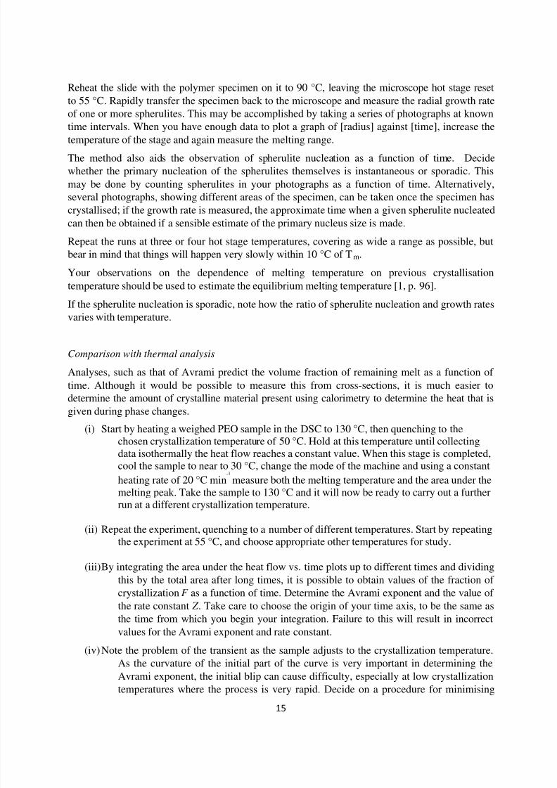
Reheat the slide with the polymer specimen on it to 90 °C, leaving the microscope hot stage reset
to 55 °C. Rapidly transfer the specimen back to the microscope and measure the radial growth rate
of one or more spherulites. This may be accomplished by taking a series of photographs at known
time intervals. When you have enough data to plot a graph of [radius] against [time], increase the
temperature of the stage and again measure the melting range.
The method also aids the observation of spherulite nucleation as a function of time. Decide
whether the primary nucleation of the spherulites themselves is instantaneous or sporadic. This
may be done by counting spherulites in your photographs as a function of time. Alternatively,
several photographs, showing different areas of the specimen, can be taken once the specimen has
crystallised; if the growth rate is measured, the approximate time when a given spherulite nucleated
can then be obtained if a sensible estimate of the primary nucleus size is made.
Repeat the runs at three or four hot stage temperatures, covering as wide a range as possible, but
bear in mind that things will happen very slowly within 10 °C of Tm.
Your observations on the dependence of melting temperature on previous crystallisationtemperature should be used to estimate the equilibrium melting temperature [1, p. 96].
If the spherulite nucleation is sporadic, note how the ratio of spherulite nucleation and growth rates
varies with temperature.
Comparison with thermal analysis
Analyses, such as that of Avrami predict the volume fraction of remaining melt as a function of
time. Although it would be possible to measure this from cross-sections, it is much easier to
determine the amount of crystalline material present using calorimetry to determine the heat that is
given during phase changes.(i) Start by heating a weighed PEO sample in the DSC to 130 °C, then quenching to the
chosen crystallization temperature of 50 °C. Hold at this temperature until collecting
data isothermally the heat flow reaches a constant value. When this stage is completed,
cool the sample to near to 30 °C, change the mode of the machine and using a constant
heating rate of 20 °C min-1
measure both the melting temperature and the area under the
melting peak. Take the sample to 130 °C and it will now be ready to carry out a further
run at a different crystallization temperature.
(ii) Repeat the experiment, quenching to a number of different temperatures. Start by repeating
the experiment at 55 °C, and choose appropriate other temperatures for study.
(iii) By integrating the area under the heat flow vs. time plots up to different times and dividing
this by the total area after long times, it is possible to obtain values of the fraction of
crystallization F as a function of time. Determine the Avrami exponent and the value of
the rate constant Z . Take care to choose the origin of your time axis, to be the same as
the time from which you begin your integration. Failure to this will result in incorrect
values for the Avrami exponent and rate constant.
(iv) Note the problem of the transient as the sample adjusts to the crystallization temperature.
As the curvature of the initial part of the curve is very important in determining the
Avrami exponent, the initial blip can cause difficulty, especially at low crystallization
temperatures where the process is very rapid. Decide on a procedure for minimising

8/3/2019 Practical Booklet
http://slidepdf.com/reader/full/practical-booklet 17/38
16
these low time difficulties and outline it in your report.
Comment on the values measured for the Avrami exponents, the crystallization mechanism
suggested, and the extent to which the results are in agreement with the microscopic observations.
How do your data support the suggestions in [5]?
Prepare a plot showing the effect of the temperature of crystallization on the subsequent crystalline
melting point. Compare your results with those obtained from microscopic observations. The heat
of melting of PEO crystals is given as between 8 and 9 kJ mol-1
monomer. [2]. Use your value for
the heat of melting of the polymer supplied to obtain a measure of its crystallinity.
Differential scanning calorimetry (DSC)
DSC measures the heat required to heat the sample at a constant rate of temperature increase. This
is compared with the heat required to heat an inert reference at the same rate. The difference in heat
flow to the sample and reference will be greatest when the sample is undergoing an endothermic
transition such as melting since extra energy is required to provide the enthalpy of melting.
The TA Instruments machine in the Polymer Characterisation Lab is a temperature flux type DSC
[6] which calculates the heat flow into or out of the sample by way of the small temperature
differences between the sample and the reference pan.
Figure 1: Schematic diagram of the DSC
Figure 2: Schematic DSC trace of a melting transition.
Crystallisation Kinetics from DSC Measurements
Microscopic observation of spherulite growth will have shown that at constant temperature the rate
of radius growth is constant with time. Where one is measuring a bulk property such as heat of
melting or sample density, the progress of crystallization will depend on (time)
3
, for if the
8/3/2019 Practical Booklet
http://slidepdf.com/reader/full/practical-booklet 18/38
17
spherulite radius is proportional to t then its volume will depend on t 3
. There are however three
provisos. The first is that the growth is spherical. If the crystallization regions grow as disks then
the dependence will be on t 2
, if it is linear, on t . Where the spherulite is formed from linear fibrils
which only branch behind the growth front, then it is an interesting issue as to whether one should
expect t 3 or linear dependence. This question may assist you in interpreting your data. The second
proviso is that all the spherulites nucleate instantaneously at t = 0, so their number remains constant
throughout the crystallization procedure. If however they nucleate sporadically at random intervals
during crystallization so that their number is proportional to time, then the degree to which the
polymer has crystallized will depend on t 4
(or if disks, t 3
). The final proviso is that as the
crystallization moves towards completion, an increasing proportion of the spherulites will grow
into each other, so that the rate of crystallization will begin to slow and eventually cease when it is
100% complete. In order to handle this effect of 'diminishing returns' Avrami (1940) introduced his
equation for the time dependence of crystallization. He showed that the fraction of material
remaining uncrystallised after time t (i.e. 1-F where F is the fraction crystallised) is given by exp [-
Zt n
]. Note that the relation at small times before significant spherulite impingement is still given by
the first two terms of the series for the exponential:
Fraction of melt remaining:
1 – F = 1 - Zt n
+ ( Zt n)2 /2! - ( Zt
n)3 /3! …………… = exp [- Zt
n]
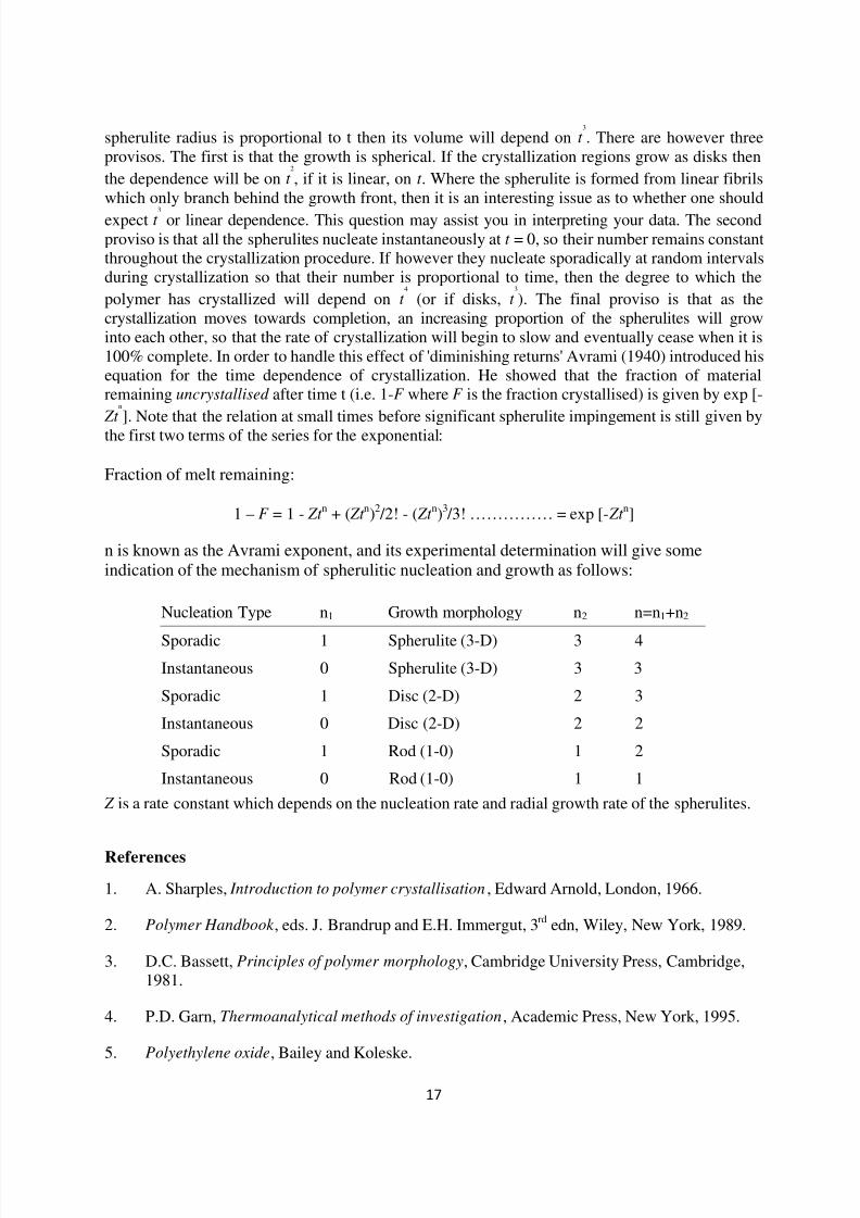
n is known as the Avrami exponent, and its experimental determination will give some
indication of the mechanism of spherulitic nucleation and growth as follows:
Nucleation Type n1 Growth morphology n2 n=n1+n2
Sporadic 1 Spherulite (3-D) 3 4
Instantaneous 0 Spherulite (3-D) 3 3
Sporadic 1 Disc (2-D) 2 3
Instantaneous 0 Disc (2-D) 2 2
Sporadic 1 Rod (1-0) 1 2
Instantaneous 0 Rod (1-0) 1 1
Z is a rate constant which depends on the nucleation rate and radial growth rate of the spherulites.
References
1. A. Sharples, Introduction to polymer crystallisation, Edward Arnold, London, 1966.
2. Polymer Handbook , eds. J. Brandrup and E.H. Immergut, 3rd
edn, Wiley, New York, 1989.
3. D.C. Bassett, Principles of polymer morphology, Cambridge University Press, Cambridge,
1981.
4. P.D. Garn, Thermoanalytical methods of investigation, Academic Press, New York, 1995.
5. Polyethylene oxide, Bailey and Koleske.

8/3/2019 Practical Booklet
http://slidepdf.com/reader/full/practical-booklet 19/38
18
6. P.J Haines, Principles of Thermal Analysis and Calorimetry, RSC, 2002

8/3/2019 Practical Booklet
http://slidepdf.com/reader/full/practical-booklet 20/38
19
P4: Casting
IntroductionThe aim of this practical is to study the effect of sodium additions (modification) on the
microstructures and impact properties of a sand cast aluminium-silicon alloy (LM6), with a
secondary aim to explore the effect of cooling rate.
Two castings of a tapered test bar of LM6 are made; one with sodium (modified), the other
without. The effects of modification and cooling rate on microstructure are investigated by
examining metallographic sections. The variation of impact strength with cooling rate is examined
by fracturing rod-like specimens that acted as risers during casting.
Sand casting
In sand casting, sifted sand (suitably moist) is packed into boxes around patterns, usually made of
wood or metal. Riser and feeder holes are cut and the boxes are assembled into the resulting mould.
Since the mould is destroyed after casting, and does not have to be preserved for subsequent use,
complex hollow shapes can be produced by using sectioned patterns, several boxes and cores, often
of sand made self-supporting, for instance by binding with linseed/synthetic oils and baking or with
sodium silicate and treating with CO2 gas.
Producing sound castings requires some skill. For instance, sufficient metallostatic head must be
provided to fill the mould completely, while the mould material must be chosen carefully to avoid
metal intrusion into pores in the sand (leading to sand burn-on) and to give good reproduction of
the pattern in the final casting. Note that in this practical, several risers are employed, in order to
obtain sufficient impact test samples.
Normally, sufficient risers and feeders are provided to allow remaining liquid metal to be sucked
back into the thickest parts of the castings as the metal contracts on solidification; the maximum
length of section that can be fed by one riser is about four times the section thickness. Adequate
provision must also be made against failure from hot shortness by providing chills to induce
directional freezing, and/or collapsible moulds which relieve the stresses on sensitive parts. The
flow of metal must be arranged so as to avoid loose sand and flux getting into the casting with the
metal, cold shuts. Also, the flow of metal must be continuous and steady. This normally means
that the cross-sectional areas of runners should be greater than the combined cross-sectional areas
of all ingates.
Experimental procedures
Safety procedures
ALWAYS WEAR THE PROTECTIVE CLOTHING PROVIDED – gloves, helmet/visors.

8/3/2019 Practical Booklet
http://slidepdf.com/reader/full/practical-booklet 21/38
20
NEVER get into a position where, if a spillage were to occur, molten metal would come into
contact with you or your clothing (including your shoes). Do not underestimate the danger of
severe burns from molten metal.
FIRST AID TREATMENT FOR BURNS – the recommended immediate treatment for burns is tosubmerge the part in cold running water; if necessary, call a First-Aider. There is a cold water tap
in the Process Area just by the Workshop door.
WEIGH OUT THE FLUXES (SEE NEXT PAGE) IN A FUME CUPBOARD.
Casting procedures
Two casting operations are to be carried out (one with modifier added and one without). In each
case, one University Crest and one tapered block are produced, the latter to be sectioned in two
locations having different thicknesses, such that they experienced significantly different coolingrates.
Quantify the water content of the Mansfield moulding sand by means of sand weight loss
measurements. Choose two pattern boxes and check they can be joined one on top of the other
using the locking pins. Place one pattern box on the board over the sandpit, and place cleaned
patterns (wedge and shield) non-centrally on the board inside the box. Lightly dust the pattern
surfaces with a releasing agent (e.g. Separit 55) or talc to ensure easy removal. Sieve sand onto the
pattern (using at first the finest sieve, and then working with progressively coarser sieves). The
sand must be hard rammed around the pattern with the wooden rods provided. Care must be taken
to avoid a layered structure in the sand, which results from one sifting of sand being completely
rammed flat before another sifting is added. Also, lightly scrape the surface of the sand before the
next sifting to aid keying. The aim in ramming is to produce good compaction below the surface,
but to leave a 10 mm layer of loose sand on top. To do this, short, sharp strokes should be used.
When the box is full, excess sand should be cut off by drawing a steel straight edge across the tip
until the sand is level with the top of the box. The assembly is then inverted so that this first box
forms the drag, i.e. the bottom box of the mould. A second box, the cope, is then placed above the
first, located with two metal rods and a pattern for the runner put on the sand surface so as to
overlap the pattern, thus forming the ingate. The appropriate surfaces are then dusted with talc, and
the cope filled with sand in the same way that the drag was loaded.
The cope and drag should now be separated and after extracting carefully the runner pattern, a
feeder hole should be cut into the cope from the far end of the runner to the top surface of the cope.
Finally, risers should be cut in the cope, using the knitting needles supplied, so as to be uniformly
spaced above the pattern in the drag. Make sufficient to provide a reasonable number for
subsequent impact testing.
The pattern should be extracted carefully from the drag and the halves of the mould left to dry
separately for about an hour before being reassembled in preparation for casing. The use of a blow
torch to aid drying may be recommended. All loose sand must be removed from surfaces that will
come into contact with molten metal.

8/3/2019 Practical Booklet
http://slidepdf.com/reader/full/practical-booklet 22/38
21
Unmodified LM6 alloy (no sodium added)
The LM6 alloy should be melted in the gas-fired furnace at a temperature of 1073 K (800 °C)
approximately. When below 1073 K, add 20 g of Coverall 11 flux followed by half a tablet of
degaser. When the melt is down to 983 K (710 °C), more flux (20 g) should be rabbled into thesurface of the melt and then the slag or dross skimmed off just before pouring at 973 K (700 °C).
Modified LM6 alloy (sodium added)
The LM6 alloy should be melted, fluxed and degassed at 1073 K (800 °C) as above. The melt
should then be modified by adding 25 g of sodium-based flux (Coverall 36A) at a temperature
between 1073 and 1023 K (800 to 750 °C). The flux should be worked into the melt for 3 minutes
before adding a further 20 g of Coverall 11. The melt should then be cooled to just above the
pouring temperature (i.e. to 983 K), fluxed with 20 g of Coverall 11, skimmed as before, and
poured at 973 K (700 °C).
Observations of castings
Examine the finished casting, complete with runners and comment on the nature and causes of any
defects you observe, and on the surface finish of the castings.
Effect of cooling rate on microstructure and impact properties
Using light microscopy on metallographic cross-sections taken from two different positions along
the lengths of both of the tapered castings, comment on the effect of cooling rate and on the
differences between the modified and unmodified structures.
To correlate impact properties with cooling rates and with modification, a Charpy impact tester is
used to fracture short lengths of unnotched risers. Examine the fracture surfaces by SEM, limiting
yourself to two samples. The matching halves of these two representative surfaces should be given
a long-term etch in NaOH solution (to dissolve the aluminium matrix) and then also examined in
the SEM. To facilitate etching, and to minimise damage to the surfaces during etching, the
samples should be mounted on aluminium stubs prior to etching and then hung upside down (with
the aluminium stubs not immersed) in a 0.05 molar NaOH solution for approximately 10-20 hours.
References
1. P.R. Beeley, Foundry Technology, Oxford: Butterworth-Heinemann, 2001.
2. W. Kurz and D.J. Fisher, Fundamentals of Solidification, Trans Tech, 1998.

8/3/2019 Practical Booklet
http://slidepdf.com/reader/full/practical-booklet 23/38
22
P5: Oxidation of Titanium in Air
Background and IntroductionTitanium and its alloys are attractive engineering materials because of their low weight, high strength
and excellent corrosion resistance [1,2]. They are used in chemical and desalination plants, in aerospace
and military applications, as fan blades in gas turbines and as medical implants. The objective of this
practical is to investigate the effect of oxidation on the metal’s hardness close to the surface. Materials
of interest are CP-Ti (titanium of commercial purity) and Ti-6Al-4V (most important titanium-based
engineering alloy).
At ambient temperature titanium has a hexagonal close- packed crystal structure, the α-phase, and upon
heating to 882 °C it transforms into a body-centred cubic crystal structure, the β-phase [1,2]. Elements
such as O, N, C and Al stabilise the α-phase, whilst transition metals such as V, Fe, Ni and Mo favour
the β-phase. By varying the type and concentration of the alloying elements, either single-phase alloys
(α or β) or two- phase alloys (α and β) can be prepared [1-4].
Titanium forms a series of oxides with different valance states, including TiO2, Ti4O7, Ti3O5, Ti2O3 and
TiO, of which TiO2 is the most stable one. The standard Gibbs free energy of formation for TiO2 is
highly negative. At 800 °C it has a value of -750 kJ mol-1
[5]. Titanium also dissolves oxygen, forming
a solid solution. At 800 °C the maximum dissolved oxygen content is as high as 14 mass% [1,2]. The
binary phase diagram of titanium and oxygen is shown in Figure 1.
Figure 1. Binary phase diagram of titanium and oxygen.
Heating titanium in air causes the formation of a layer of metal oxides at the surface and a layer of
oxygen-enriched metal underneath. This layer has a typical thickness of a few hundred microns and is
known as the α-case. The term α-case is derived from the fact that the α-phase prevails in the oxygen-
enriched surface of titanium alloys that consist of primarily the β- phase or both the α-phase and the β-
phase. The α-case forms during extensive machining, hot processing or long-term service at elevated
temperature in air. It is hard and brittle and can cause serious deterioration of the metal’s performance,
especially its fatigue properties [6].
8/3/2019 Practical Booklet
http://slidepdf.com/reader/full/practical-booklet 24/38
23
The oxygen content of the α-case in titanium can be estimated from measured hardness values. A
quantitative correlation between Vickers hardness and oxygen concentration in CP-Ti is given in
Reference [7]. The transport of oxygen into titanium is controlled by diffusion and therefore leads to a
typical oxygen concentration profile within the α-case. The functional correlation between oxygen
profile and oxygen diffusivity is found for instance in Reference [8].
Basic experimental work
• Experimental work includes: the formation of the α-case on foils of CP-Ti and Ti-6Al-4V by heating in air, the investigation of the α-case using microhardness measurements and
light optical microscopy.
• Equipment provided includes: foils of CP-Ti and Ti-6Al-4V, refractory wires and various
tools, a programmable furnace, a thermocouple with read-out unit, a mounting press,
grinding and polishing wheels, a light optical microscope, a microhardness tester.
Experimental procedures
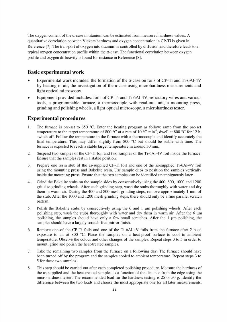
1. The furnace is pre-set to 650 °C. Enter the heating program as follow: ramp from the pre-set
temperature to the target temperature of 800 °C at a rate of 10 °C min-1
, dwell at 800 °C for 12 h,
switch off. Follow the temperature in the furnace with a thermocouple and identify accurately the
final temperature. This may differ slightly from 800 °C but should be stable with time. The
furnace is expected to reach a stable target temperature in around 30 min.
2. Suspend two samples of the CP-Ti foil and two samples of the Ti-6Al-4V foil inside the furnace.
Ensure that the samples rest in a stable position.
3. Prepare one resin stub of the as-supplied CP-Ti foil and one of the as-supplied Ti-6Al-4V foil
using the mounting press and Bakelite resin. Use sample clips to position the samples verticallyinside the mounting press. Ensure that the two samples can be identified unambiguously later.
4. Grind the Bakelite stubs on the sample sides by consecutively using the 400, 800, 1000 and 1200
grit size grinding wheels. After each grinding step, wash the stubs thoroughly with water and dry
them in warm air. During the 400 and 800 mesh grinding steps, remove approximately 1 mm of
the stub. After the 1000 and 1200 mesh grinding steps, there should only be a fine parallel scratch
pattern.
5. Polish the Bakelite stubs by consecutively using the 6 and 1 μm polishing wheels. After each polishing step, wash the stubs thoroughly with water and dry them in warm air. After the 6 μm polishing, the samples should have only a few small scratches. After the 1 μm polishing, thesamples should have a largely scratch-free mirror finish.
6. Remove one of the CP-Ti foils and one of the Ti-6Al-4V foils from the furnace after 2 h of
exposure to air at 800 °C. Place the samples on a heat-proof surface to cool to ambient
temperature. Observe the colour and other changes of the samples. Repeat steps 3 to 5 in order to
mount, grind and polish the heat-treated samples.
7. Take the remaining two samples from the furnace on a following day. The furnace should have
been turned off by the program and the samples cooled to ambient temperature. Repeat steps 3 to
5 for these two samples.
8. This step should be carried out after each completed polishing procedure. Measure the hardness of
the as-supplied and the heat-treated samples as a function of the distance from the edge using the
microhardness tester. The recommended load for the hardness testing is 25 or 50 g. Identify the
difference between the two loads and choose the most appropriate one for all later measurements.

8/3/2019 Practical Booklet
http://slidepdf.com/reader/full/practical-booklet 25/38
24
For the present samples, the thickness of the α-case should be less than, or on the order of, 100
μm. Make 10 indentations in an area similar in size to that indicated in Figure 2. Arrange theindentations diagonally away from the sample edge, bearing in mind that the distance between
neighbouring indentations should be at least three times greater than the diagonal line of the
indentation.9. Inspect the samples under the light optical microscope. Describe the visual appearance of the
samples and record a set of representative images.
Figure 2. Indentation pattern on the α-case of a ground and polished titanium sample.
Analysis of results
• Describe the changes that occur to the CP-Ti and Ti-6Al-4V samples during heat
treatment in air.
• Plot the hardness measured in the α-case of the CP-Ti and Ti-6Al-4V samples as a
function of the distance from the edge for the different heat treatments, and discuss why
the hardness profiles for CP-Ti and Ti-6Al-4V differ.
• Plot the oxygen contents in the α-case of the CP-Ti samples as a function of the distancefrom the edge for the different heat treatments, and estimate the diffusivity of oxygen in
CP-Ti at 800 °C.
References
[1] A.D. McQuillan and M.K. McQuillan, Titanium, Butterworths Scientific Publications,
London, 1956.
[2] R.I. Jaffee and H.M. Burte (Editors), Titanium Science and Technology, Plenum Press,
New York, 1973.
[3] I.J. Polmear, Light Alloys: Metallurgy of the Light Metals, 3rd Edition, John Wiley &
Sons, New York, 1995.
[4] V.A. Joshi, Titanium Alloys: An Atlas of Structures and Fracture Features, CRC Press,
Boca Raton FL, 2006.
[5] A. Roine, HSC Chemistry for Windows, Outokumpu Research Oy, Pori, Finland, various
editions and release dates.

8/3/2019 Practical Booklet
http://slidepdf.com/reader/full/practical-booklet 26/38
25
[6] R.W. Evans, R.J. Hull and B. Wilshire, The effects of alpha-case formation on the creep
fracture properties of the high-temperature titanium alloy IMI834, Journal of Materials
Processing Technology, 56 (1996) 492-501.
[7] G.Z. Chen, D.J. Fray and T.W. Farthing, Cathodic deoxygenation of the alpha case ontitanium and alloys in molten calcium chloride, Metallurgical & Materials Transactions B,
32 (2001) 1041-1052.
[8] T.K. Roy, R. Balasubramaniam and A Ghosh, Determination of oxygen and nitrogen
diffusivities in titanium aluminides by subscale microhardness profiling, Scripta
Materialia, 34 (1996) 1425-1430.

8/3/2019 Practical Booklet
http://slidepdf.com/reader/full/practical-booklet 27/38
26
M1: Woods
AimAfter examining this group of samples you should be familiar with the basic structures present
within wood and the way the structures respond to tensile and compressive deformation.
Samples
You are supplied with samples of balsa (a low density hardwood), oak (a medium density
hardwood), spruce and pine (both of which are softwoods). The samples include thin sections and
bulk samples, suitable for a stereo microscope and the SEM. These are coated with a conductive
coating of either silver or gold.
Look at the samples supplied and determine the essential features of the structure of wood, relating
the two dimensional sections to what can be seen in the bulk samples. Discuss how these vary inthe different woods and how wood deforms and breaks. Begin by studying either oak or spruce and
then compare this with the other samples that are available.
References
1. See articles in the Journal of Microscopy 104 [1], May 1975, especially the first article by
J.M. Dinwoodie. This is provided in a folder, next to the samples.
1. CRC Handbook of Materials Science, Vol IV: Wood , Eds R. Summitt and A. Sliker.
2. L.J. Gibson and M.F. Ashby, Cellular Solids: Structure and properties, Chapter 10, 2nd
Edition,
Cambridge University Press.
8/3/2019 Practical Booklet
http://slidepdf.com/reader/full/practical-booklet 28/38
27
M2: Biomedical Materials
Aim
After examining these samples, you should be familiar with the nature of materials and their failurein hip joint replacement prostheses and also be familiar with the way in which bone is able to grow
into and around bioactive implants.
Introduction
This Material Examination practical is split in to two parts. The first part requires you to observe
retrieved hip prostheses and to try to investigate why they failed in service. For the second part of
the practical you are asked to study histological slides of bioactive implants into which bone has
grown and you are required to assess how much bone integration has occurred, using standard
measurement techniques. You may need some assistance with the measurement techniques and Dr
Judith Juhasz [email protected]
1. Failed Implants
will be available to explain the background if required.
The replacement of old, damaged or diseased bone is now an established procedure, an estimated
40 000 hip replacements are performed annually within Britain alone. Unfortunately, many of the
procedures fail and approximately 18-20% of the operations performed each year are revisions
operations. The problems may sometimes be due to the patient’s response to the implant, but in a
small number of instances, they may be due to failure of the component itself.
You are supplied with three components of hip replacement prostheses retrieved from patients after
they failed in service.
Specimen 1 is ultra high molecular weight polyethylene (UHMWPE) acetabular cup that in normalservice in a hip prosthesis acts as the bearing surface in the pelvis (in the acetabulum).
Specimen 2 is the proximal (upper) portion of a failed cobalt-chrome femoral stem with the ball
joint of the femoral component attached.
Specimen 3 is the femoral stem of titanium alloy hip prosthesis. The yellowish / white material
along the length of the femoral stem is a poly(methyl methacrylate) (PMMA) based bone cement.
It would have been used to fix the implant to the bone.
Acetabular cup
Observe the acetabular cup and identify the various components that are attached to it. Describe the
function of the components and the cup as a whole. Observe the different types of damage thathave occurred in the different areas of the cup and describe these. Describe the type of damage that
has occurred to the polymer and discuss the likely course of events that led to the failure of the
implant.
Femoral Stem
The majority of metal implants for bone and joint replacement are based on three major alloy
types, namely austenitic stainless steel, cobalt-chromium and titanium alloy. In general, optimum
properties correspond to a minimum grain size and minimum porosity, while uniform properties
are generally associated with a uniform grain size distribution.

8/3/2019 Practical Booklet
http://slidepdf.com/reader/full/practical-booklet 29/38

8/3/2019 Practical Booklet
http://slidepdf.com/reader/full/practical-booklet 30/38
29
view frame is then calculated from:
100%)Area(
t
1 ×=∑=
=
P
H n x
x
x
(1)
where H is a hit, n the number of hits and Pt is the total number of points on the grid. Repeated
counting at different areas of the specimen is usually advised to improve the accuracy of the
estimate.
Linear intercept methods are generally used to quantify surface features such as bone coverage.
Lines are superimposed on the image and a hit is regarded as a place where a line intersects a
feature. As before, measurements are made on a number of fields until an accurate estimate is
obtained. Different types of grid are available. They are typically composed of straight lines, a
notable exception being a Merz grid which comprises alternating semicircles which build up a
wave pattern.
You will be provided with histological micrographs for two different samples. Both are images of
porous hydroxyapatite granules that have been used to fill a drilled defect in bone. One of the
images has been taken after the granules have been in the bone for a period of six weeks and the
other image is for implants that have been in place for 12 weeks. The aim of this part of the
Materials Examination practical is for you to assess the amount of bone that has grown in between
the granules and also the amount of bone that is in direct contact with the granules.
Percentage of Bone Ingrowth
Measure the percentage of bone ingrowth using the micrographs superimposed with a Weibel grid
and choose four different quadrants (bold squares) in which to make your measurements.Count a hit for bone ingrowth (HBI) wherever a point falls over an area of bone. The percentage of
bone ingrowth within the implant is calculated using Equation 2
( )100
42
1BI
BI ×=∑
=
=
n x
x j
H
AZ (2)
Calculate the result for both the 6-week and the 12-week implants. Comment on your answer.
Coverage of Bone on Implant Surfaces
Measure the coverage of the bone on the implant surface using the micrographs superimposed
with a Merz grid and choose four different quadrants (bold squares) in which to make yourmeasurements.
A hit for bone coverage (HBC) is scored where a line intersects a bone:implant interface. Similarly
a hit for implant: space (HIS) is scored where a line intersects an implant:space interface. The
percentage of implant surface covered by bone within the zone (ZBC) is then given by Equation 3
and the value of bone coverage for the each of the quadrants can be calculated.

8/3/2019 Practical Booklet
http://slidepdf.com/reader/full/practical-booklet 31/38
30
ZBC
=
H BC i( )i=1
i= x
∑
H IS j( )+ H BC j( ) j=1
j= y
∑ j=1
j= y
∑× 100 (3)
As with your calculation of bone ingrowth, evaluate the area percentage of coverage within each of
the quadrants. What do you notice? How does the bone fill the implant? Calculate average values
for the 6-week and 12-week samples and describe the change in bone ingrowth and coverage with
time.
References
Biomaterials Science, Eds. Ratner, Hoffman (This book has information about materials used in a
range of different biomedical implants).

8/3/2019 Practical Booklet
http://slidepdf.com/reader/full/practical-booklet 32/38
31
M3: Brazing and welding
AimAfter examining these samples, you should be able to recognise and understand the structures that
form during brazing and welding of materials. Brazing is where a molten metal is used to join two
pieces of metal that remain solid (similar to soldering). In fusion welding, not only is there a molten
material that joins the two pieces, and which is used to fill the join, but a small region of each of
the pieces of parent material also melts. See the references for sources of information on the
various joining techniques, details of which do not have to be included in your write-up except
where some aspect clearly affects the observed microstructures.
Samples
HA Normalised low-C steel, silver soldered with Cu-Ag-Cd solder (etch: FeCl3)
What is the inherent basis of the joining process used and why might it be used? What is the
microstructure of the silver solder and suggest how it might have arisen?
HB Friction weld in mild steel (etch: 2% nital) How does the macroscopic appearance of the
joint relate to the friction welding joining process?
What are the characteristic features of the joint microstructure? What type of steel is the parent
metal?
HC Resistance spot weld in clad Al-alloy sheet (etch: 5% HF) How does the weld microstructure
reflect the welding process used? What can be observed about the parent material?
HE Submerged-arc weld, bead on plate, in steel (etch: 2% nital)
wt.% Fe C Mn Si S P Al Nb Cu
plate: balance 0.25 0.52 0.02 0.005 0.042 0.008 0.08 0.12
weld: balance 0.15 0.70 0.26 0.014 0.038 0.020 0.06 0.19
wire: balance 0.11 0.97 0.23 0.022 0.021 0.007 0.01 0.35
Unaffected parent material
Describe the microstructure in terms of the phases you can see and the grain size (is it coarse or
fine?) How directional is the microstructure? Can you deduce anything about the finish-rolling
temperature from this?
Heat - affected zone (HAZ)
What is the HAZ? Estimate its width. What different regions can you see in the HAZ? Account for
their formation with reference to the iron-carbon phase diagram. (It is suggested that you work
from the parent metal to the weld metal.)

8/3/2019 Practical Booklet
http://slidepdf.com/reader/full/practical-booklet 33/38
32
Weld metal
How would you describe the white phase on the grain boundaries and what might it be? Which
phases are typical of a high-heat-input microstructure? Is there a difference between the carbon
content of the parent and the weld metal? What type of cracking has occurred and how could it be
prevented?
HX Brazed silicon carbide joint
This joint between two blocks of hot pressed silicon carbide has been brazed with Ticusil, a
commercial Ag-Cu-Ti braze, Ag – 26.5 wt% Cu – 4.5 wt% Ti. The brazing process was
performed under vacuum. The sample has been polished to a 1 μm finish and is carbon coated.
The presence of titanium in the braze composition encourages wetting of the braze on the
silicon carbide surfaces.
The brazing operation was as follows:
Heating from room temperature to 750 °C at 10 °C min−1, dwell at 750 °C for 10 min, heating
from 750 °C to 950 °C at 10 °C min−1, dwell at 950 °C for 20 min, followed by cooling at 10
°C min−1 to 750 °C, then 5 °C min−1 to 500 C and finally 2 °C min−1 to room temperature.
Examine the joint by optical microscopy and scanning electron microscopy (SEM). Why is the
joint best examined by SEM? Examine the joint by secondary electron imaging and by back
scattered electron imaging. Which imaging mode is more useful for this specimen. Why? What
can you deduce about the microstructure of the braze?
Use the Ag-Cu-Ti ternary phase diagram provided below to specify the form of the brazeliquid at 950 °C. Examine the Ag-Cu binary phase diagram to determine what braze
microstructure you would expect in the absence of titanium in the braze. Hence or otherwise
infer what happens to the microstructure when titanium is added to the braze composition.

8/3/2019 Practical Booklet
http://slidepdf.com/reader/full/practical-booklet 34/38
33
Figure 1 Liquidus surface of the Ag-Cu-Ti ternary phase diagram
References
Joining processes:
1. Ideally Level 3 and the select Process Universe in Cambridge Engineering Selector
(CES) available on the Class computers. This software may also be down-loaded from
the Department’s web site (but only has Level 2 which does not include submerged arc
welding): www.msm.cam.ac.uk/Teaching/ces/index.html
2. Wikipedia
Background information
K.E. Easterling, Introduction to the Physical Metallurgy of Welding, Butterworths 1983.
R.W.K. Honeycombe and H.K.D.H. Bhadeshia, Steels: Microstructure and Properties, Arnold,
London, 1995.
Lancaster, Metallurgy of Welding, George Allen & Unwin, 4th edition 1987.

8/3/2019 Practical Booklet
http://slidepdf.com/reader/full/practical-booklet 35/38
34
Welding Handbook (several volumes), American Welding Society, currently 8th edition.
ASM Metals Handbook , Vol. 6 -Welding, Brazing and Soldering, ASM 1993.
Engineered Materials Handbook , Vol. 4 - Ceramics and Glass, Section 7: Joining, ASM 1991.
G. Humpston and D.M. Jacobson, Principles of Soldering and Brazing, ASM 1993.

8/3/2019 Practical Booklet
http://slidepdf.com/reader/full/practical-booklet 36/38
35
M4 — Fracture Mechanisms
Aim
To introduce basic fracture mechanisms occurring under a range of conditions in different materials.
Introduction
You will have used and heard a number of terms used to describe failures in materials: Brittle Fracture,
Ductile failure Micro-void coalescence, cleavage, inter-granular, trans-granular, fast fracture, etc.
Many of these terms are not mutually exclusive but can mean different things in different contexts. For
example, take the term ductile; a ductile failure might be characterised macroscopically by a thinning of
the gauge length of the sample, i.e. ‘necking’, the two halves of such a failure would not fit back
together. On a micro-scale we could also look for signs of ductility on the fracture surface. For
example where a fracture has occurred by the coalescence of voids there might be localised yielding of
the filaments between the voids yet on a macro-scale the surface fit together perfectly. Is this failure
ductile or brittle?
When examining fracture surfaces first look at the sample with your eye; there are many features
clearly visible to the eye, which simply cannot be seen in the microscope. Has large-scale deformation
occurred, can you fit the pieces together (don’t damage the fine detail by ramming then together) can
you see discrete areas of the fracture surface which are a different colour. Is the surface oxidised or
corroded does this give you a clue as to the timescale of the fracture. As you move to the microscopekeep a mental map of the fracture surface and work from a low magnification to high so that you know
where the fine detail is located within the fracture. Try to identify the initiation point of the crack and
the areas which failed last and most rapidly, these can be completely different.
In particular we need to distinguish between micro and macro-mechanisms of failure. i.e. those we can
see and form conclusions from with the naked eye and those for which an optical or electron
microscope is necessary. The aim of this practical is to introduce you to some real fracture surfaces
some of them quite complex and to recognize features on the macro and micro-scale so that you are
able to interpret what is going on and possibly suggest what might be done to avoid or delay failure.
There are not necessarily right or wrong answers.
Samples
1. F3 Tensile failure in Copper at room temperature
This specimen displays a classic ductile failure mode. Examine and describe the macroscopic
shape of the fracture surface and think where the failure started. Look at the central part of the
fracture in the SEM for signs of micro-void coalescence. Try looking at the steep sides of the
‘cone’, how does this differ from the centre. Describe the sequence of events during the failure.

8/3/2019 Practical Booklet
http://slidepdf.com/reader/full/practical-booklet 37/38
36
2. F5. Polycrystalline zinc broken by impact at room temperature.
Macroscopically the fracture surface shows large flat facets across the grains indicative of failureby cleavage. Microscopically you should be able to distinguish parallel cleavage planes and the
transition between them. Zinc is hexagonal close packed metal. What do you think the cleavage
planes might be? Why does zinc undergo brittle failure at room temperature in contrast to the
copper sample.
3. F9: Single crystal superalloy (CMSX-4) Tensile failure at 850°C.
Examine the un-mounted end of the test-piece, is the failure brittle or ductile? What is the micro-
mechanism of failure? Compare the fracture surface with the cleavage surface of the zinc. Look for
evidence of plasticity e.g. change in the diameter of the gauge length, slip lines on side of sample.
4. F10 High temperature fatigue failure in IN738, A cast, polycrystalline, Ni-based Superalloy.
IN738 is a cast polycrystalline Ni-based superalloy used for turbine blades principally in the energy
business. The grain size is ~1mm. Polycrystalline superalloys contain small amounts of carbon, the
carbides formed strengthen the grain boundaries. This sample has been subjected to Low Cycle
Fatigue at 850°C to simulate the changing stresses experienced by the blade in service and has
failed.
Look at the whole of the fracture surface under low magnification in the SEM, can you identify any
sites where the fracture might have initiated? Bearing in mind the average grain size of >1mm and
the cast nature of the material what might the relief on the surface relate to? Now look at higher
magnification. It is worth looking at this sample using the Backscattered Electron mode, BEI
(compo). This will reveal differences in the atomic number of the material and hence will show
local variations in composition. Can you see a second phase at the fracture surface? This may
suggest what determined the fracture path. Compare different regions of the sample. Although this
is a fatigue failure no striations are visible in this sample. See reference 1.
5. F7: Fatigue crack propagation in Udimet 720 – Tested at room temperature.
Udimet 720 is a nickel based superalloy used for gas turbine disks, the material is cast, forged at
high temperature and recrystallises during this process. It contains a large volume fraction of
coherent γ’ precipitates to improve high temperature properties. However, in the very high stresses
experienced at the crack tip in the plastic zone, these precipitates have the effect of concentrating
the slip on just a few planes, so called ‘in-homogenous slip’. This can show up in as a fracture
surface which is roughly facetted.

8/3/2019 Practical Booklet
http://slidepdf.com/reader/full/practical-booklet 38/38
Look at the sample by eye and identify different zones moving away from the notch. In the SEM
examine the surface and look for any features in each of the zones. Do you think the testing was
the same throughout the test? Compare this to the fracture surface formed during the later (and
more rapid) stages of the crack propagation. You may be able to see facets closest to the notch
where the crack growth rate is lowest. In this sample you should be able to identify striations on
the fracture surface. See reference 1.
References:
1. ASM Metals Handbook Vol. 19 [R135] See Antolovich, p. 854. for sample F7, and p. 489 for
sample F10.
2. Anderson, Fracture Mechanics Fundamentals and Applications, 2nd
Ed. CRC press, (1995). See
p.265 and 282 for general introduction to ductile and brittle behaviour and section 6.3.1 is of use for
sample F12
3. Engel and Klingele, An atlas of Metal Damage, Wolfe Publishing Ltd. [MB191]
The demonstrator on this series is Dr. Soran Birosca, and he can be contacted at [email protected] for
assistance.


![Unit 3 Practical Skills Booklet B *GBL32* [GBL32] ONDAY 17 ...](https://static.documents.pub/doc/80x56/61c76c0b076e2a11b769893c/unit-3-practical-skills-booklet-b-gbl32-gbl32-onday-17-.jpg)


