Master programme in Economic Demography Pre- and post-migration labour market mismatch in Sweden 1970-1990 Martin ¨ Onnerfors [email protected]Abstract Labour market outcomes for immigrants in general is a well researched field, but the mechanisms behind labour market mismatches among immigrants post- migration is still in need of empirical research. Using a unique and newly compiled dataset on Swedish immigrants, also containing pre-migration occu- pational and educational information data, this study aims makes use of maxi- mum likelihood models to measure the influence of an individual’s pre-migration history on the post-migration outcomes. The results show significant associa- tions between pre- and post-migration mismatch status, and a persistence in the mismatched state over time. Possible explanations include individual abil- ity, discrimination, imperfect transferability of human capital, and changes in labour demand. The method used is not causal, and the associations shown should be researched further using a causal approach. Keywords: educational mismatch, labour market integration, immigration, Sweden EKHM52 Master thesis, second year (15 credits ECTS) June 2016 Supervisor: Kirk Scott Examiner: Kerstin Enflo Word count: 17.670
Transcript
Master programme in Economic Demography
Pre- and post-migration labour marketmismatch in Sweden 1970-1990
Labour market outcomes for immigrants in general is a well researched field,but the mechanisms behind labour market mismatches among immigrants post-migration is still in need of empirical research. Using a unique and newlycompiled dataset on Swedish immigrants, also containing pre-migration occu-pational and educational information data, this study aims makes use of maxi-mum likelihood models to measure the influence of an individual’s pre-migrationhistory on the post-migration outcomes. The results show significant associa-tions between pre- and post-migration mismatch status, and a persistence inthe mismatched state over time. Possible explanations include individual abil-ity, discrimination, imperfect transferability of human capital, and changes inlabour demand. The method used is not causal, and the associations shownshould be researched further using a causal approach.
Keywords: educational mismatch, labour market integration, immigration,Sweden
EKHM52Master thesis, second year (15 credits ECTS)June 2016Supervisor: Kirk ScottExaminer: Kerstin EnfloWord count: 17.670
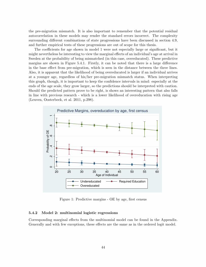
1 Predictive margins - OE by age, first census . . . . . . . . . . . . . . . . . . . . 44
3
1 Introduction
The success or failure of immigrants on their host country labour markets is an increasinglydiscussed topic today. Crises in, and inequalities between, different parts of the world aredriving migration flows to increasingly high levels. In light of the large global disparities inprosperity and influence, some researchers consider even the high levels of recent years to bemodest, compared to what might theoretically be the case (Massey et al. 1999, p.7).
The modern Swedish history of immigration and labour market integration has gonethrough periods of labour migration, refugee migration, as well as economic boom and bust.Along with the economic crisis of the 1990s came a structural change of the economy that putfurther demand on host country-specific skills for immigrants (Rosholm, Scott, and Husted2006). There are, in other words, both supply and demand forces at work in shaping labourmarket outcomes for immigrants in Sweden. In order to succeed in labour market integration,policy needs to be aptly designed to handle these issues.
Labour market mismatches, meaning that an individual’s acquired education does notmatch with the required education for his/her occupation, is an issue that can be costly tosociety. When it comes to the unfavourable form of mismatch (overeducation), the state ispaying via education costs and loss of efficiency, and the overeducated individual by lesserlabour market outcomes and emotional cost (Piracha, Tani, and Vadean 2012). Generally,labour market mismatches are more common among immigrants (Leuven, Oosterbeek, et al.2011), and this is also the case for the Swedish labour market (Joona, Gupta, and Wadensjo2014).
A common problem in researching labour market outcomes for immigrants in general, andmismatches in particular, is that most often, pre-migration data is not available. Informa-tion on an individual’s occupational and educational history is important when trying to findexplanations for observed outcomes, but for most studies, only post-migration data is avail-able. This study uses a unique data source on Swedish immigrants, providing informationon pre-migration education and occupation, and allows for taking this important piece of theexplanation into account when studying labour market mismatches in Sweden.
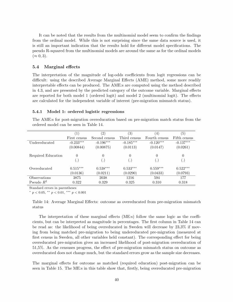
Using this newly complied data source of immigrants arriving to Sweden between 1970and 1990, the objective of this thesis is to know more about what role an individual’s pre-migration history might have in explaining post-migration labour market mismatches. Thestudy adds to the field both by contributing knowledge on the Swedish situation using uniquepre-migration information, but also to the general field, by producing results that can beadded to a field in need of empirical research.
1.1 Research question
This thesis aims to answer the following research question: does an immigrant’s pre-migrationlabour market mismatch influence the possibility of being mismatched in the Swedish labourmarket? If an association is found, what is the direction and magnitude?
1.2 Outline
This thesis is organised as follows: first (section 2), a theoretical framework and previousresearch on the possible aspects of immigrant labour market mismatches are presented. Sec-
4
tion 3 will go through the data used, and in section 4, methods and econometric models arediscussed. Descriptive results, and later the results from the models, are presented in section5, and synthesised with the hypotheses in section 6. The final discussion of the findings isfound in section 7.
2 Theory and previous research
The study of labour market outcomes for immigrants is a field of research that incorporatesmany sub-fields. Even without introducing the complexity of an individual’s trajectory beforearriving in a new country, there are still many different theories concerning what predictslabour market outcomes. With the added information of an individual’s pre-migration history,the mechanisms become even more complicated. Since many perspectives are needed to coverthe possible explanations for the labour market mismatches of immigrants, this theory sectionwill draw from three fields of research: firstly (section 2.1), theory and results from generalstudies on labour market mismatches, and secondly (section 2.2) theory and results on generallabour market outcomes of immigrants. The third field (section 2.3) presents studies on thecombined subject of labour market mismatches among immigrants. Finally (section 2.5), thepresented research is used to construct hypotheses and a priori expectations.
2.1 Labour market mismatches
A labour market mismatch can arise from a number of sources. An income mismatch existswhen a person’s income deviates from what can be expected for the current occupation. Ahorizontal educational mismatch exists when the field of a person’s education deviates fromthe field of the current occupation. The most commonly researched, and also the one that isthe focus of this paper, is the vertical educational mismatch. This type of mismatch is definedas a discrepancy between the level of education acquired by a person, and the required levelof education for this person’s current occupation. In general, the state of overeducation isthe most researched. Overeducation can be argued to be of greater policy interest, in thesense that it is associated with costs for both state (providing the education) and individual(monetary and emotional cost). This section will give an overview of the existing theoreticalperspectives on vertical mismatches, and common results from previous research in the field.
2.1.1 Human capital theory
The definition, and even the possible existence of a labour market mismatch, depends on one’stheoretical perspective. An influential work by Gary Becker (1964, Human capital) defines thewage outcome of a worker as representative of the worker’s marginal productivity (Sala et al.2011, p.1027). In this framework, even if a worker has more education than what could beconsidered as required, the wage reflects the true value of the worker’s productivity (withoutmarket imperfections). By this definition, no mismatches can exist. According to McGuin-ness (2006, p.387), the interest for labour market mismatches, and educational mismatches inparticular, was brought to real interest by Richard Freeman’s study of the US labour marketin 1976. In this study, it was concluded that the declining returns to education among Ameri-can college graduates was due to excess supply from general overeducation. Even though thisstudy did not consider overeducation at the individual level, but rather as a market collapse,
5
it drew the attention of researchers (Sala et al. 2011, p.1026).
The seminal work by Mincer (1974) introduces the human capital earnings function, whichhas become widely used within economics. Using this function, an educational mismatch canexist within the Human Capital framework: according to Mincer’s model, surplus schoolingexists as a compensation for a lack of work-specific human capital McGuinness (2006, p.390).In this sense, educational mismatch can be viewed as a problem of omitted variables. Ingeneral, Human Capital theory can be argued to view educational mismatches mostly as ashort-term problem of insufficient human capital, if the concept is at all recognized.
2.1.2 Job competition theory
Job competition theory was introduced by Thurow (1975), and it puts the demand side of thelabour market in command of an individual’s outcomes. According to this theory, prospectiveworkers are put in a queue and ordered by how much on-the-job training would be required tomake them productive. A highly educated worker is always selected before a lower-educatedworker, which means that if the supply of workers is higher than the demand, overeducatedworkers will be selected. Since the employer sets the wage according to the job characteristics,not the individual characteristics, the overeducated worker then ends up with a wage penalty(Tsai 2010, p.607).
2.1.3 Job assignment theory
Where Human Capital theory focuses on the individual’s characteristics, and job competitiontheory on the occupation’s characteristics, job assignment theory does a bit of both. The the-ory was introduced by Sattinger (1993), and it empathises the interplay between the worker’schoice of a job/sector and how wages are set. In job assignment theory, a wage outcome isinfluenced both by a worker seeking to maximise utility, and an employer seeking a certainkind of worker (McGuinness 2006, p.398). An educational mismatch according to this theorycan arise from both the individual and the job, thus leaving the field open for explanationsincluding individual ability as well as the characteristics of the occupation.
2.1.4 Career mobility theory
Complementing the different theoretical perspectives on mismatch, Sicherman and Galor(1990) presented a general theory on mobility in the labour market. Introducing the ”proba-bility of promotion” for a worker within the current company (ibid., p.177), the theory makesit possible to regard overeducation as a first career step. In other words, being overeducatedin a short-term perspective in the beginning of your career is considered rational. The au-thors also theorise that overeducation could stem from a worker compensating his/her lackof job-specific human capital. Since both formal and informal human capital are needed tobe qualified for an occupation, a worker with excess formal education need not necessarilybe overqualified, considering the demands for informal on-the-job skills (Robst 1995, p.539).In a test of the career mobility theory using longitudinal data, Buchel and Mertens (2004,p.803) argue that their results ”cast serious doubts” on the ability of career mobility theoryto explain the presence of overeducation. Considering the data used in this thesis, the ca-reer mobility theory can not be fully utilised, since all individuals have had a job prior to
6
migration. It could, theoretically, be argued that the ”starting over” that faces immigrantspost-migration is comparable to a native’s first job, but it would be harder to find a crediblestrategy to identify this using the data at hand. This theory will, therefore, not be consideredin the hypotheses.
2.1.5 Signalling and screening
Within the signalling theory, the value of a persons’s education does not necessarily lie in theeducation itself, but in the signal that the completed education sends to a potential employer:a signal of higher productivity. So, education increases earnings not because it increases aperson’s productivity, but because it signals that a person is ”..cut out for ’smart’ work.”(Borjas 2005, p.241). According to the signalling theory, the potential employee invests bothdirect and opportunity costs to acquire the right signalling towards an employer, but this isdependent on the potential wage benefit exceeding the cost (Weiss 1995). As the signallingtheory takes the employee’s perspective, the screening theory takes the employer’s perspectiveon the same concept, assuming that the employer uses acquired education level to screen andfilter among applicants. The education level can then be seen as a proxy for (often unobserved)positive individual characteristics, such as productivity (Arrow 1973).
2.1.6 Previous results
The empirical research concerning outcomes from labour market mismatches came into focusagain (after a spell of lower interest during the 1970s) with an article by Duncan and Hoff-man (1981). This article introduced the ORU model (Overeducation - Required education- Undereducation) that is a modified version of the human capital earnings function (Min-cer 1974), and the ORU model is now commonly seen in empirical research on mismatches.The results from Duncan and Hoffman (1981) showed that the returns to one extra year ofovereducation are positive, although only half of the premium that comes from adding an-other year of required education (that is, education pays off better while employed on in anoccupation with the same required education as the acquired). In general, many studies seemto come to this conclusion: overeducation is associated with a wage penalty (compared tothe correctly matched workers of the same education), and this penalty is costly in manyperspectives (Leuven, Oosterbeek, et al. 2011, p.290). The cost is carried both by individualand state, to different degrees, depending on the educational system. In later years, however,many researchers have started to question these findings. Two issues are often brought up asproblematic: the self-selection problem, and the measurement-error problem, and these willbe discussed below.
2.1.7 Self-selection and ability
Much of the research that finds wage penalties from overeducation are based on the OLSmodel, which often suffers from identification issues when used in this field. The classicalproblem of non-random assignment to treatment means that it is impossible to know if it’svariation in the independent variable or variation in the error term that is affecting the out-comes variable (Angrist and Pischke 2008, p.12). The widely used ORU model introduced byDuncan and Hoffman (1981), when used in combination with OLS, is no exception to thatrule (Leuven, Oosterbeek, et al. 2011, p.304). Up until quite recently, these issues have been
7
more or less overlooked (Leuven, Oosterbeek, et al. 2011). The use of standard OLS to modellabour market outcomes from mismatches has been heavily criticised by some researchers(Tsai 2010, Korpi and Tahlin 2009, Pecoraro 2014), and methods such as IV or fixed effectshave been employed to try and get rid of the apparent omitted variable bias.
It can be argued that who ends up in an overeducated state and who is correctly matched isnot a random process, but is influenced by the individual’s characteristics (such as the com-monly mentioned ”innate ability”). If this is the case, the labour market outcome of a workercan not be argued to only come from the mismatched state itself, but might as well come fromvariation in ε. Using individual fixed effects to account for this individual ability, Tsai (2010)aims to find outcomes that have not been influenced by self-selection. Her results suggest thatthe proposed wage penalty from overeducation disappears when individual effects are beingcontrolled for. This is interpreted by the author as an indication of the real reason behindthe wage penalty being selection into overeducation by lower-ability workers (ibid., p.611).
Pecoraro (2014) mentions the same critique regarding omitted ability variables. He addressesthe issue using a fixed effects approach, but also tries to control for ability bias in an OLSsetting using a proxy variable (ibid., p.311). The proxy variable consists of the differencebetween the expected and the realised wage for an occupation. Using this variable needsthe assumption that the set wage measures a worker’s individual productivity/ability that isunrelated to the acquired education. This method was first used by Chevalier (2003), andboth Chevalier and Pecoraro reach the conclusion that there is indeed negative selection onability into overeducation.
2.1.8 The measurement-error problem
The second issue that is often mentioned concerning the identification of mismatch outcomesis measurement errors in the variable of interest. The fact that a mismatch variable consistsof a difference between two schooling level variables (acquired and required education) makespotential measurement errors an even bigger problem than if schooling were used as a sin-gle variable (Leuven, Oosterbeek, et al. 2011, p.306). Also, using a fixed-effects frameworkto account for unobserved factors may inflate the error even further, since the fixed-effectsframeworks are known to be unforgiving towards measurement errors (Angrist and Pischke2008, p.168).
The case of these measurement errors has been discussed and approached in different ways.Tsai (2010, p.613) is aware of the fact that her fixed-effects results could be argued to be dueto measurement-error bias. Both a numerical approach and survey data are used to test thesensitivity of the results, and Tsai finds that the results hold. These tests are, however, ques-tioned by Leuven, Oosterbeek, et al. (2011, p.309), who argue that they are not shown to beconsistent. Verhaest and Omey (2012, p.77) also discuss the measurement problem at length,and note that the bias in overeducation outcome studies usually is directed downwards. Thiswould mean that the wage penalties usually found are understated.
A common strategy to combat measurement-error bias in mismatch models is to instrumentdifferent types of mismatch variables on each other. Robst (1994) uses this technique and
8
finds that the wage penalty is even higher than first estimated. Verhaest and Omey (2012,p.86) also use the technique, combined with a fixed-effects model, and find that measurementerror is a substantial source of downward bias. A problem with the IV approach as correctorof measurement error is, as pointed out by Leuven, Oosterbeek, et al. (2011, p.308), thatit only applies when the measurement error is classical (that is, when the measurement er-ror is uncorrelated to the true mismatch value). In many cases, it can be argued that themeasurement error is non-classical, which means that IV correction will not eliminate thebias.
2.2 Labour market outcomes for immigrants
Separate from the impact of labour market mismatch in general, labour market outcomes forimmigrants is an area of research by its own right. Early works of Barry Chiswick found resultsindicating that immigrant wage outcomes are significantly lower than natives, but that theycatch up and eventually surpass native earnings (Chiswick 1978). The initial dip in earningsis attributed to a lack of country-specific human capital, which is said to be acquired withgrowing labour market experience. The approach and conclusions by Chiswick were criticisedby Borjas (1985), who argued that Chiswick’s results are a product of his cross-sectional ap-proach, and that the results more likely come from differences between cohorts. Borjas finds,instead, that the ”quality” of the cohorts are different, with the earlier cohort being of higherquality. This leads to a situation that might look like an improvement with more years spentin the host country, when it is actually the earlier cohort having a higher quality than the later.
In later years, this field of research has widened considerably, and many explanations forimmigrant outcomes have come into focus. In this section, theories and results concerningthe potential mechanisms behind immigrant labour market outcomes will be presented anddiscussed.
2.2.1 Selection into migration
Self-selection is an important issue in most parts of empirical microeconomics and this is alsocertainly true for the study of migrants. A model to analyse self-selection into migrationwas developed by Borjas (1987), based on the notion that people who migrate can not beexpected to be chosen at random. The model presented by Borjas includes a framework toanalyse the mechanisms behind positive and negative selection on skills (and other factors).The outcomes from this selection process depend on a number of factors: the transferabilityof skills, the income distribution in the source country, and the returns to education in bothsource and host country (Rooth and Saarela 2007, p.91). The combination of these sourcescan create a selection that is very specific: for example, a host country can attract migrantsthat are negatively selected on observable skills (low education), but positively selected onunobservable skills (high ability). Return migration, which also has a large effect on thecomposition of migrants in the host country, can be argued to be driven by the same forcesthat drive the selection into first migration (ibid.).
Concerning the current state of selection into migration in the OECD countries, Belot andHatton (2012) conclude that positive selection on education has more to do with low physicaland cultural distance than the usually mentioned wage incentives. Also, having a colonial
9
legacy in a source country lowers the poverty constraints that usually block poorer peoplefrom migrating (Belot and Hatton 2012, p.1125). In the case of Sweden, Rooth and Saarela(2007) find that Finnish immigrants are negatively selected on education, since returns toeducation for highly educated Finnish workers are higher in Finland than in Sweden.
2.2.2 Discrimination
An important factor affecting the labour market outcomes of immigrants is ethnic discrimi-nation in the labour market. The observed ethnic income gap in Sweden means a -15/-22%wage penalty for southern EU/non-EU second generation immigrants, compared to natives(Nordin and Rooth 2009, p.488). Together with Denmark and Belgium, Sweden has the high-est ethnic employment gap in the OECD countries (OECD 2015, p.69). In theory, these gapsin labour market outcomes can arise from discrimination, but also from unobserved individualheterogeneity, and the nature of the discrimination issue makes it especially difficult to showempirically that it exists.
Trying to find evidence of labour market discrimination in Sweden, Carlsson and Rooth (2007)construct an experiment using fake job applications with ethnic/native-sounding names beingthe variation of interest. They find large differences in callback rates, where Middle Eastern-sounding names names receive as much as 50% less callbacks. The authors discuss the po-tential mechanisms behind the results, but cannot safely say which type of discrimination isbehind. On the same topic, Nordin and Rooth (2009) exploit military enlistment intelligencetests as a proxy for individual ability to identify discrimination. Their results suggest thatethnic discrimination in Sweden affects employment possibilities, but not wages (p.504). Thisis attributed to either labour market discrimination and/or unobserved variables (p.496).
2.2.3 Labour demand
The demand side of the labour market for immigrants affects both labour market outcomesand migrant flows. The paper by Borjas (1985) emphasises changes in the supply side (cohortquality) but does not rule out a ”fall in demand for immigrant labour” (p.485). In lateryears, the interplay between macro-economic fluctuations and immigrant outcomes have beenthe focus of several studies. Dustmann, Glitz, and Vogel (2010) research the labour marketresponses of immigrants during economic downturns in the UK and Germany. These two coun-tries are shown to have large differences in immigrant population composition, both regardinglevels of education and countries of origin (p.4). These differences might in turn produce dif-ferences in outcomes. Dustmann et al. find, however, similar responses to economic crisis inboth countries, as lower-educated immigrants experience a heavier employment penalty thanhighly educated immigrants. The main immigrant outcome from economic downturn (in bothcountries) is higher unemployment, not lower wages (p.14).
A similar study on the Scandinavian labour market was presented by Rosholm, Scott, andHusted (2006), where different immigrant cohorts in Denmark and Sweden are followed on thelabour market. Similar to the results of Dustmann et al., labour market outcomes in the twocountries show a common pattern, despite the differences in unemployment patterns duringthe study years (p.335). The results show that immigrants in both countries experienced
10
declining opportunities in employment during the study period (1985-1995). The authorspresent the theory that this decline is due to a change in the labour market structure (thedemand side), shifting to a market that is more demanding in terms of informal human cap-ital and country-specific skills. The change can be described as the switch from ”Fordism”to ”Toyotaism” (Helgertz 2010). Similar results are found by Bevelander and Nielsen (2001),who use a decompositional method to find sources of variation in the Swedish immigrant-native employment gap. They find that the deteriorating employment conditions for Swedishimmigrants between 1970-1990 arise from changes in unobserved variables rather than whatcan be observed using regular socio-economic variables (p.463). These unobserved variablesare suggested to be labour market discrimination, or the same structural changes pointed outby Rosholm, Scott, and Husted (2006).
2.2.4 Transferability of human capital
Education and experience that has been acquired abroad does not always hold its value ina new country. Transferability of human capital for migrants can be an issue, as quality ofschools, educations and certificates might differ between countries. Also, cultural and lin-guistic distances between source and host country can have an effect on this process in bothdirections.
Friedberg (1996) makes a distinction between formal human capital (years of education)acquired abroad and domestically in her article on Israeli immigrants. It is found that humancapital is imperfectly transferred between countries, but that the rate of portability varies withcertain groups of countries. Immigrants to Israel from ”Europe and the Western Hemisphere”have higher rates of return to their pre-migration human capital than do migrants from Africaand Asia (p.246). Friedberg theorises that this might be due to differences in school quality,or discrimination. It is also found that the returns to labour market experience acquiredabroad is insignificant in general. Chiswick and Miller (2002) study foreign-born men fromnon-English speaking countries in the US, and find that English language proficiency has asignificant positive effect on wage outcomes. The concept of linguistic distance (meaning howfar away an immigrant’s mother tongue is from the host country language, linguistically) isused as a measure of ”skill transferability”. Also, it is found that living in a ”linguisticallyconcentrated area” has a negative effect on wage outcomes (ibid., p.49). In the case of Swe-den, Helgertz (2013) researches the impact of linguistic distance of immigrants on their labourmarket outcomes (in the years 1970-1990). The results show that an increasing linguistic dis-tance is associated with negative labour market outcomes: proficiency in a language fromthe Germanic language family gives an advantage in the likelihood of acquiring a job (ibid.,p. 462). There does not, however, seem to be any large differences between the non-Germaniclanguages. Judging from the results from ibid., language skills are important in order tosucceed in the Swedish labour market during the study period (which is also the study periodin this thesis).
2.3 Mismatches among immigrants
The combined topic of labour market mismatches among immigrants is generally underre-searched, but on the rise (Piracha, Tani, and Vadean 2012). The field exists in the cross-
11
section between the mismatch literature (section 2.1) and the literature on immigrant labourmarket outcomes (section 2.2), and carries with it the complexities from these two fields.Depending on one’s choice of outcome variable, different theories and results have been pre-sented. Regarding incidence, it is generally reported that immigrants have a higher degreeof educational mismatch than natives (Chiswick and Miller 2008, Leuven, Oosterbeek, et al.2011, Piracha, Tani, and Vadean 2012). Possible explanations as to why immigrants experi-ence labour market mismatches are individual ability (section 2.1.7), selection into migration(section 2.2.1), first-job tenure (section 2.1.4), discrimination (section 2.2.2), signalling (sec-tion 2.1.5) and language/transferability (section 2.2.4).
There are two studies on the subject that are of special importance in relation to this thesis:the study on pre- and post-migration mismatch mechanisms in Australia by Piracha, Tani,and Vadean (ibid.), and the study of mismatch outcomes and state dependence of Swedishimmigrants by Joona, Gupta, and Wadensjo (2014). The first study utilises data collected byAustralian authorities, in a similar manner to the SLI database used in this thesis (describedfurther in section 3.2). The authors use signalling as their hypothesis for why immigrantscould experience both pre- and post-migration mismatch. The signalling proposed is not aneducation signal, but a signal from the most recent employment pre-migration (Piracha, Tani,and Vadean 2012, p.2). A notable difference between Sweden and Australia is the Australianmigration policy implemented in 1995, described as the ”skill stream” of migrants. Througha point system, a large share (around 50% in 1999) of the migrants accepted into Australiaare graded according to the benefit they could bring to the country, which puts emphasis onoccupational experience and language skills (Miller 1999, p.193). Since ”business skills” andreferences are important in the point scheme, the migrants accepted will need to have thisformally in order, which makes the signalling theory more likely. It is, on the contrary, likelythat some groups of migrants (such as refugees) will have a harder time producing the neces-sary work credentials in order for signalling to take place. The results from this study showthat the existence of a pre-migration mismatch is the strongest predictor of a post-migrationmismatch, after controlling for a number of demographic and occupational variables (theseresults are compared to the findings of this thesis in section 6). The authors attribute the re-sults to ”ability signals” from the pre-migration mismatch status (Piracha, Tani, and Vadean2012, p.19).
The second study by Joona, Gupta, and Wadensjo (2014) focuses on the post-migration mis-match outcomes of immigrants in Sweden. By using a rich source of register data, individualsare followed over time in order to know more about the possible differences in state depen-dence of mismatches. The previous research presented by the authors suggests that there isindeed a strong state dependence within overeducation, but that the potential heterogeneouseffects between natives and immigrants are underresearched (ibid., p.4). With regards toincidence of mismatches among Swedish immigrants, the authors find a higher incidence ofovereducation among immigrants compared to natives (p.10). State dependence is modelledusing a dynamic random effects model with Mundlak correction, and the results show a veryhigh degree of state dependence in overeducation in general, for both natives and immigrants.Immigrants, and especially non-Western immigrants, have even higher rates than natives,which is attributed in part to imperfect transferability of human capital (p.20). In contrast tothis thesis, Joona, Gupta, and Wadensjo (ibid.) do not have access to pre-migration mismatch
12
data, so there can be no direct comparison of results, but the study is still a good indicationof the Swedish labour market experience for immigrants.
2.4 Swedish immigration history
Prior to the Second World War, immigration to Sweden was mainly made up by NorthAmerican return migrants. After the Second World War, Sweden had an intact infrastructureand industry, and simultaneously, demand grew for raw materials to re-build Europe. Growingdemand increased the pressure on the industry, and made the Swedish government recommendan increased inflow of labour migrants of around 10.000 per year (Helgertz 2010, p.3). The firstcohorts to arrive in the 1940s and 1950s were labour migrants, but later, inflows of politicalasylum seekers began to arrive: political instability in Greece, Poland, Chile and Yugoslavia(amongst others) led to refugees becoming the dominant part of the migrant stock. ForPoland, the repression of the Jaruzelski regime made immigration to Sweden peak in 1982,and for Chile, the years just after the 1973 military coup marked the height of immigration toSweden (Klinthall 2007, p.584). In recent years, apart from work and study migrants, wavesof immigration have come consisting of refugees from crises in Iraq, Afghanistan and Syria,with following waves of tied movers (SCB 2016a).
2.5 Hypotheses
Following the presented theory and results, a number of a priori expectations can be stated. Asa clarification, it should be mentioned that the topic and research question of this thesis modelsa mechanism that is not the most commonly researched: the relation and persistence of amismatch over time, with the intermediate disturbance of an international migration. Much ofthe existent theory and research on mismatches focuses on a secondary labour market outcome,such as wage, and not the existence and persistence of the mismatch per se. This means thatthe validity of comparison of these theories and results with the research question in this thesiscan be discussed. In order to make use of the theories and results, it is necessary to make thecomparison: higher wage and higher employment can be considered ”better” labour marketoutcomes, which ≈ less likelihood of overeducation. The five proposed hypotheses are:
• H1 - signalling : the effect of a ”pure” (randomly assigned) pre-migration mismatchcan be theorised to transfer from pre- to post-migration via signalling, which wouldmanifest through a higher likelihood of a post-migration mismatch from a pre-migrationmismatch.
• H2 - individual ability : if a pre-migration mismatch can be theoretically attributedto individual ability, the presence of a pre-migration mismatch should make a post-migration mismatch more likely. Since ability can be considered time-invariant, thiseffect should also be constant over time.
• H3 - discrimination: if labour market discrimination can be argued to contribute neg-atively also to matching, a general shift downwards (i.e. undereducated → requirededucation or overeducated, required education → overeducated) would be an outcomefrom arriving in Sweden for some groups of immigrants.
13
• H4 - labour demand : if lower labour demand for immigrants also affects mismatchstatus, a higher likelihood for downwards shift will be visible in cohort effects for yearsof boom or bust.
• H5 - transferability : considering the heterogeneity between countries of origin, immi-grants from different countries are expected to have different likelihoods of mismatchbased on different levels of transferability and linguistic/cultural distance. Also, thelikelihood of overeducation is expected to decline with increasing years since migration,as country-specific human capital is accumulated.
These hypotheses will be commented on using the results from this thesis in section 6.
3 Data
There are two principal data sources behind this thesis. For data on the Swedish side, officialSwedish data sources such as the tax registry and 5-year censuses have been used to constructa panel dataset for each individual. This dataset includes income, civil status and internalmigrations, all of which are data and events occurring in Sweden (post-migration).
For the pre-migration information, the Swedish Longitudinal Immigrant database (SLI)has been used. This database consists of a sample of immigrants to Sweden starting in1968, and was collected continuously until 2005 (Helgertz 2010). From the SLI, a randomsample of 17.074 individuals is the base sample for this thesis. The SLI is a unique sourceof pre-migration information, and contains information on origin, education, occupation andlanguage. For this particular research question, the information on pre-migration occupationis of special importance: this variable allows for the construction of a pre-migration mismatchstatus, which is rarely seen in this field of research. As mentioned in section 2.3, the datasource used in Piracha, Vadean, et al. (2013) and Piracha, Tani, and Vadean (2012) is tothe author’s knowledge the only comparable source containing this information. This sectionwill describe how variables of interest have been constructed, and how the final sample wasselected.
3.1 Sample
As stated previously, the SLI sample contains 17.074 individuals to begin with. After removingindividuals without a job title, without data on acquired education and whose job titles couldnot be matched against the official list of Swedish occupational titles (SSYK), 8.848 individualsremain. Also, individuals with previous occupations in the military sector (ISCO code 0, table3) were excluded, since the military occupational field does not operate in the same way asthe rest of the labour market. 17 individuals with inconsistent information on birth year(more than one unique year present) were also removed. Before joining the SLI data to anyadditional data, the sample size is 8769 individuals (the removal progress can be followed intable 1).
There are some additional aspects of the sample that need to be handled when modelling.Already mentioned are the military occupations, but there are also other special groups:occupations within performing culture and sports are very hard to assign a believable requirededucation, since one can reach higher levels within these fields both with and without higher
14
Reason for removal Count Left in sample
Original sample 17074
No data on occupation (pre-migration) 3886 13188
No data on education (pre-migration) 2055 11133
Not matched against SSYK 2285 8848
Military sector 62 8786
Conflicting birth years 17 8769
Table 1: Sample size
education. Individuals who were self-employed prior to migration might not be representative,since they can be considered to have a higher likelihood of starting their own business also inSweden, which would put them outside the regular labour market. Furthermore, individualsoutside the age range of 16 to 54 at arrival in Sweden can not be considered representative:the younger individuals might receive education in Sweden, and the older individuals have ahigher likelihood of entering directly into retirement (Helgertz 2010, p.40). These categories(individuals within performing arts or sports, self-employed, and outside the age range) willbe excluded from the main model results, but included in as a part of sensitivity tests (section5.5).
3.1.1 Censuses
Income data from the tax register was joined to the SLI without losing any individuals fromthe sample. Information on occupations and civil status, however, are only present in the5-year censuses. Censuses are available, for this thesis, for the years 1970, 1975, 1980, 1985and 1990. These censuses are the data points available for following migrants in Sweden,and as migrants arrive continuously during the study period, many different combinations ofpresence in data are possible. Table 2 contains the number of individuals present on numberof censuses. This number of individuals corresponds to the final sample used for modelling,and thus excludes the categories mentioned in section 3.1, and also individuals with missingdata.
Number of censuses present 1 2 3 4 5
Individuals 3875 2038 1216 594 181
% of final sample 100,00% 52,53% 31,34% 16,93% 4,66%
Table 2: Number of individuals per census
As seen in the table, 3875 individuals are present in at least one census (this one beingtheir first), and only 181 individuals are present for all five censuses. ”Present” is defined ashaving a mismatch status, which implies being employed at the time of census. Note that thiscan be in any of the five censuses - when modelling, all data is evaluated at time of census andthe individuals are pooled from different immigration cohorts. No individual appears twicewithin one census, but individuals are followed over time in as many censuses as possible.
15
3.2 Pre-migration data
The SLI pre-migration data contains title of occupation for every individual before migratingto Sweden. This information has been collected by the Swedish immigration authority duringmeeting concerning permits (Helgertz 2010). The occupational title information was hand-typed and contained numerous spelling errors. In order to clean and synthesize the presentoccupations, the hand-typed data were matched against the SSYK (SCB 2016c). During thematching, a Levenshtein string distance score was calculated between the two sources, andthis was used to facilitate the subsequent manual work of finding a correct occupational titlefor each pre-migration title. In total, around 3500 unique strings were matched.
3.2.1 Required education
In order to calculate a mismatch, information on required education for an individual’s currentoccupation is needed. There are several methods that can be used to obtain this (presentedin Leuven, Oosterbeek, et al. 2011):
• self-assessment : individuals are asked how much education they believe is needed toperform (or be recruited to) their current job. The advantage of this approach is thatit is gives a direct insight in the requirements, but workers might also be misinformedabout or exaggerate how much education is needed.
• job analysis: this approach makes use of the existing international (and national) oc-cupational classifications (for example, ISCO), in which a required education for eachoccupation has been decided upon. Using this technique might give more consistentresults, but might also remove valuable heterogeneity.
• realised matches: making use of the already employed individuals within an occupation,it is possible to calculate a representative education from these. Both the mean andmode education within an occupation have been used by different researchers. Using anumerical variable such as years of education, the definition of a mismatch has often beendefined as +/- 1 σ from the mean, which can be argued to be an arbitrary definition.Also, this method has been criticised for only reflecting the supply/demand forces andnot a true general required education (ibid., p.293).
Since the SSYK (which has been matched against the SLI occupation titles) also containsa required education for each occupation (originating from the ISCO-08 classification), thejob analysis approach would be a first suggestion for the current data. In the case of theSLI, however, which contains immigrants from many different countries, the job analysismethod was deemed inappropriate. At closer inspection of the data, it was found that specificcountries and occupations contained heterogeneity that would have created bias if disregarded:for example, more than 90% of the nurses from Iran in the SLI sample had a secondaryeducation, while the SSYK/ISCO classification dictates that being a nurse requires a post-secondary education. If job analysis were used here, almost all Iranian nurses would turn outas mismatched, even though it can easily be argued that this is probably not the case. Theself-assessment method was impossible to use, since data had already been collected, so therealised matches method was chosen to compute the required education.
16
Code Group
1 Managers
2 Professionals
3 Technicians and associate professionals
4 Clerical support workers
5 Service and sales workers
6 Skilled agricultural, forestry and fishery workers
7 Craft and related trades workers
8 Plant and machine operators, and assemblers
9 Elementary occupations
0 Armed forces occupations
Table 3: ISCO-08 major groups
3.2.2 Creating the required education-variable
In order to best capture the nature of an occupation within the country context that it exists,the matched and cleaned occupation titles from SLI were grouped by title and country, andfrom these groups, the mode education was selected. The chosen cut-off group size was 10individuals. If an occupation had less than 10 individuals within a country, it was groupedon title and country-group. And, if title and country-group was not enough, the remainingrequired educations were chosen using country groups and the 10 ISCO ”major groups” (listedin table 3). These ISCO groups exist with the SLI data as a part of the connected SSYKclassification, and consist of a broad classification of occupations, both horizontally (sector)and vertically (level of management).
The share of individuals classified with each method is listed in table 4. The distributionthese individuals, as shown per the calculated required education, is fairly stable across thesample. A deviation can be seen in the ”Countrygroup+ISCO”-method group, which has alarger share of post-secondary individuals. This can be explained by the fact that there existsa larger number of unique occupation titles in the higher spectrum of the education scale (inSSYK, 51% of the titles are at post-secondary level, and only 15% at primary level). Thismeans that there are more titles to group by in the higher end, and less chance of passing the10-individual cut-off.
Table 4: Percentage of individuals by classification method
3.2.3 Acquired education
The SLI information on an individual’s acquired education prior to migration is available inseveral variables: years of education (numeric), vocational education (free-text) and educationcategory (free-text). The ”years of education” variable turned out to be unusable, since data
17
was missing for 43% of the individuals. The ”education category” variable, however, is presentfor 81% of the individuals and contains the three education groups ”Primary”, ”Secondary”and ”Post-secondary”. This variable is used as the acquired education level for individualsprior to migration. The variable ”vocational education” contains free-text information thatwas found to be too incoherent for use in this analysis. For example, 78% of the nurses inthe sample have information in this variable, but there are 37 different strings containing theinformation just for this occupation. Since the cleaning of this data would be manual for themost part, there was not enough time in this project to make use of this information.
3.3 Constructing a mismatch variable
To construct a vertical educational mismatch variable, two components are needed: acquirededucation level of an individual, and the required education level of the current occupation ofthe same individual.
The variable is computed according to this scheme (AE = acquired education, RE =required education):
AE > RE = Overeducation
AE = RE = Matched
AE < RE = Undereducation
For the pre-migration data, the distribution of educational mismatches can be seen in Table5. The distribution of the pre-migration mismatches shows an amount of mismatches that issimilar both over and under the ”required education” level. These figures differ somewhat fromthe corresponding distribution presented by Piracha, Tani, and Vadean (2012), where only 8%of the migrants where overeducated, and 24% where undereducated before migrating. Thesefigures, however, reflect the underlying Australian immigrant policy, which is selective towardshighly educated immigrants (ibid., p.8). A higher degree of undereducation is therefore tobe expected in Australia compared to Sweden, where the immigration policy does not favourhighly educated migrants (Klinthall 2007).
Pre-migration mismatch status Individuals % individuals
Overeducated 630 16,26%
Required Education 2775 71,61%
Undereducated 470 12,13%
Sum 3875 100,00%
Table 5: Pre-migration mismatches
The mismatch variable should also be broken down on other variables: table 6 contains thedistribution of pre-migration mismatches by acquired education (also pre-migration). Firstly,it can be noted that there are no overeducated individuals with primary education, and noundereducated individuals with post-secondary education. This is by definition of the vari-able. It is noteworthy that only 12,7% of the correctly matched individuals have a secondaryeducation, which indicates that this educational category is more prone to mismatches. Thiscan be seen better in the column-wise percentages in Table 7.
Table 6: Pre-migration mismatches by acquired education
From this table, it is obvious that the secondary education level has a higher share ofmismatches than the primary and post-secondary levels. Given, the secondary class can bemismatched in both directions, but it is still noteworthy that the majority of individuals inthis education class is mismatched. This issue is discussed further in section 3.5.
Mismatch status Primary Secondary Post-secondary
Overeducated 40,69% 23,68%
Required Education 86,30% 37,12% 76,32%
Undereducated 13,70% 22,19%
100,00% 100,00% 100,00%
Table 7: Pre-migration mismatches by acquired education - column-wise percentages
For a small number of individuals, two occupations were reported. In these cases, therewill only be a deviation in case the two occupations has different required educations (whichwas the case for 147 individuals). For these cases, the highest required education was chosento compute the mismatch status (but models were also run using the lowest, see section 5.5).
3.4 Post-migration data
The post-migration data from the Swedish registries is generally straightforward to use. Mostof the data used is constructed as long panels, where demographic events, such as migrationsand civil status changes, are recorded with an exact time-stamp. As data was processed andselected, a number of decisions had to be made: firstly, the data was down-sampled to ayearly basis. In the case of individuals changing their citizenship, civil status, or residenceseveral times during a year, only the last event within the variable was used. Secondly,repeat migrations were considered: if an individual immigrates to Sweden, emigrates, andthen immigrates again, the ”years since immigration” variable will only count the years spentin Sweden. Generally, peculiar edge cases that were found (such as multiple birth/deathdates) were dropped, but these were very few in total (<50).
3.4.1 Required education
The required education for an occupation in Sweden is provided by SCB as part of the census,via the socioeconomic classification variable SEI (SCB 2016b). This variable, however, wasnot delivered with the 1970 and 1975 censuses. To mediate this problem, the SEI scoresfrom the 1980/1985/1990 censuses were used to calculate a mode value (using the ”realisedmatches”-method as described in section 3.2.2). This calculation, compared to the calculationon pre-migration data, did not suffer from lack of observations, and no lower threshold wasneeded (the three censuses together contain >750.000 observations). The method might create
19
a bias, arising from the potential difference in educational attainment within occupations overtime in Sweden (but this can be considered to be low-risk, since the periods are close in time).
3.4.2 Country of origin
Distribution of country of origin for all individuals in the sample can be seen in Table 8.Countries that had a very low number of individuals (<10) have been excluded from the sample(examples of these countries are Eritrea, Russia, Bosnia and North Vietnam). Germany hasbeen chosen as the base category for modelling, since it is well represented in the sample andculturally close to Sweden.
Table 8: Pre-migration mismatches by country of origin
3.4.3 Metropolitan place of residence
All Swedish municipalities have an urban status category of metropolitan/non-metropolitan,which is delivered by SCB. The metropolitan municipalities are the ones in and around thethree largest cities in Sweden (Stockholm, Goteborg and Malmo), and the distribution ofindividuals in the sample on this status can be seen in Table 9. Since around 17% of thetotal Swedish population lives in these three cities (SCB 2015), it is clear that living in ametropolitan area is overrepresented in the sample. There does not seem to be, however, anyskewed representation within the mismatch categories.
Table 9: Pre-migration mismatches by residence status
3.5 Data issues and bias
Concerning the data used, there are several issues that might compromise the validity andreliability of the results:
20
• precision of census data: an important restriction on the data used in this thesis isthe interval between censuses. These censuses are only performed every five years,which means that individuals have time to switch jobs several times between censuses.According to the figures of Joona, Gupta, and Wadensjo (2014), around 14% of Swedesswitch jobs each year, but with no significant differences in frequency between nativesand immigrants. Theoretically, this could bias the results in both directions, and it isonly the jobs both that come and go between two censuses that pose the real issue, asthese may be changing the mismatch status. There is unfortunately little to be doneabout this issue other than keep it in mind when interpreting the results.
• overrepresentation in secondary education: As shown in section 3.3, there seems to bean overrepresentation of educational mismatches in the ”secondary education” category.It is, by definition, possible to be mismatched in both directions in this educationalcategory, but it is also possible that there might be a larger inherent likelihood ofbeing mismatched being in this category - due to unmeasurable labour market variables.As noted in section 5.5, different cut-off values for the mismatch variable generationhave been tried but this did hardly influence the mismatch distributions. The possiblebias arising from this overrepresentation is thus hard to demonstrate, or to predict indirection.
• attrition: the panel data sample suffers from attrition of several kinds: mortality/oldage retirement, outmigration and unemployment. Out of the three, mortality/retirementattrition is the least problematic, since it is likely to be random enough for the purposesof this thesis. Concerning outmigration, however, there is good reason to suspect thatthis is not random (as discussed in section 2.2.1), and it is reasonable to expect thatindividuals experiencing failure in the labour market are more likely to emigrate. Thiswould bias the likelihood of overeducation downwards, in the theoretical case that theseindividuals still were on the labour market. The problem of only considering employedindividuals (under which the unemployment attrition falls) is discussed closer in section5.6.
• measurement error : as discussed in section 2.1.8, mismatch variables are especiallysensitive to measurement errors, since both errors in the acquired and required edu-cation variables can influence the result. As for the required education variable (pre-migration), sensitivity tests using different cut-offs have been tried, without finding anydifferences. The pre-migration acquired education and occupation information is self-reported, and it is possible that these suffers from social desirability bias. This type ofbias is mostly mentioned in cases of self-reported data concerning behaviour and polit-ical views (Kaminska and Foulsham 2013), and is therefore considered low-risk in thecase of this thesis. The post-migration data on occupation and education used in thisthesis is Swedish registry, which usually is considered to be of high quality.
• post-migration education: when calculating mismatch status, both pre- and post-migration,the acquired education level pre-migration is used. However, it is possible that individu-als educate themselves further in Sweden, but data on this has not been available in thisthesis. If a large number of individuals were to re-educate themselves in Sweden andthereby change education category, this could bias the results upwards, and overestimatethe likelihood of being overeducated.
21
• vocational data: as mentioned in section 3.2.3, free-text information on an individual’scompleted vocational education was not included because of time constraints. Somerudimentary inspection of the data shows that the vocational title in most cases seem tocorrespond to the acquired education level entered (i.e. doctors having post-secondaryeducation) - but more time would be needed to confirm that this holds for all of thesample. Depending on how common it is to report non-corresponding combinations (i.e.primary education + doctor), this issue can lead to an overestimation of the likelihoodof being overeducated.
4 Method
The research question states that it is the probability of experiencing a labour market mis-match that will be the outcome variable of the analysis. This phenomenon is identified withthe categorical mismatch variable (described in section 3.3), where the post-migration mis-match status will be used as dependent variable, and the pre-migration mismatch status beingthe independent variable of interest.
To answer the research question, two models are proposed: Model 1 uses an ordered lo-gistic regression setup, and Model 2 uses a multinomial regression setup. Both models havean associative approach rather than causal, and the endogeneity problems connected to thesemodels are discussed in section 4.4. In this section, the theoretical foundation of the methods(logistic regression and the ML estimator) will first be presented, and then the specificationsof the two models.
4.1 Logistic regression
When estimating using probabilities using a linear model, the probability of an event yi|xioccurring can go below 0 or above 1. In a Logit model, this does not occur, since a distri-butional assumption is made about the probability distribution of yi: common choices arethe standard normal distribution (probit) or the standard logistic distribution (logit). In thispaper, the logit model will be used as a starting point, but sensitivity tests using the probitmodel will also be made (section 5.5).
Defining the function of interest as w = x′iβ, the logistic distribution function is given by:
F (w) =ew
1 + ew
Defining the probability of yi = 1 as pi = P (yi = 1|xi), the log odds ratio of an event canthen be defined as:
logpi
1− pi= x′iβ
4.1.1 Ordered logit models
Using an ordered model for categorical data makes sense if the categories have an inherentorder that can be exploited. The idea can be explained using the existence of a latent variable
22
y∗ that controls the transition between the categories. In a simplified case, this latent variablecould for example be individual ability, which can be argued to influence labour marketmismatches. The latent variable (which is unobserved) can be defined as y∗i = x′iβ + ui,without an intercept (Cameron and Trivedi 2010, p.519). As the value of y∗i increases, theprobability of yi taking a certain value changes (Verbeek 2008, p.210). For example, if abilitycould be measured on a scale from 0 to 12, the threshold points between overeducated andmatched / matched and undereducated could lie at 4 and 8. This would give the logic:
y∗i < 4→ yi = overeducated
4 <= y∗i < 8→ yi = matched
y∗i >= 8→ yi = undereducation
As the outcome of the ordered logit is interpreted, it can be referred to coefficients asbeing results of an increase in the underlying latent variable. In this case, that would mean ahypothetical ability increase (hypothetical, since ability is often seen as constant) that wouldresult in a change in the mismatch status.
The ordered logit model uses the assumption of proportional odds between the categories,which means that the probability distributions for each of the outcome variable categories areassumed to be identical (Long and Freese 2006, p.151). This assumption is tested in section5.2.3.
4.1.2 Multinomial logit models
In contrast to the ordered logit model, a multinomial model does not assume that there is amonotonic latent variable behind the choice of category, instead, the categories are treated asindependent and mutually exclusive (Verbeek 2008, p.229). When calculating the probabili-ties, coefficients are usually interpreted in relation to a base category in the outcome variable,but base probabilities can be predicted for all categories using marginal effects methods. Afrequently mentioned issue with multinomial models is the Independence of Irrelevant Al-ternatives (IIA), which is a situation that can arise when two or more alternatives in thedependent variable have the same practical implication. A common example of this is thechoice between travelling by train, blue bus, or red bus - choosing one of the latter alternativeswould imply a high utility also for the other (ibid., p.230). For the variable used in this thesis,however, this will not be an issue: the dependent variable is not a choice variable, and thecategories are mutually exclusive by definition of the variable. Using a multinomial modelwill provide a different angle on the data, by not locking the outcome variable to an ordinalform. If there is variation that does not fall into the pre-defined ordinal pattern of risingability/labour market success, it should be captured by a multinomial model.
4.2 Maximum Likelihood estimator
A non-linear limited dependent variable model is often modelled using a Maximum Likelihood(ML) estimator (ibid., p.211). The choice between Linear Probability Models, LPM (usingOLS estimator), and ML estimators in limited dependent variable models depends on contextand the underlying data-generating process, but it is also an issue of some debate. Using
23
OLS gives access to many of its wanted characteristics (for example, easier interpretation ofmarginal effects), but it has also been argued that it gives inconsistent estimates in limiteddependent variable models (Horrace and Oaxaca 2006). In this thesis, an ML estimator willbe used.
The ML estimator gets its name from the fact that once a probability distribution for theoutcome is assumed, this function is maximised to give the most likely value of β (in a regres-sion setting). Instead of estimating a value for y, an ML estimator estimates the likelihoodthat y takes a certain value. In general, the ML principle builds on the notion that a randomvariable y has a probability density function that depends on a set of unknown parametersθ, which gives the function f(y|θ). If n observations from this process can be argued to beindependent and identically distributed (IID), the joint density function can be written as:
f(y1|θ) =
n∏i=1
f(yi|θ)
This is then the product of the individual densities (Greene 2003, p.509), and is called thelikelihood function. It is often written as L(θ|y), with θ first, which is to indicate that we areinterested in the unknown function behind the values of y that we can observe. This functionis unobservable and a part of the data-generating process, but using our measured values of y,we can estimate it. Usually, the logged version of this likelihood function (the log-likelihood)is used, since it is then easier to maximise (Verbeek 2008, p.180). In a regression setting,where we also have independent variables (in a matrix X), the log-likelihood function can bewritten as:
logL(θ|y,X) =n∑
i=1
logf(yi|xi, θ)
Since the log-likelihood function allows for summing probabilities.
4.3 Average marginal effects
Marginal effects (ME) are a way to make the magnitude of coefficients more tangible, and sincethe coefficients from non-linear estimators are harder to interpret than those of linear models,marginal effects are often needed to say something about magnitude. A marginal effect canbe defined as the change in conditional mean of y as an independent variable changes by oneunit (which can also be described as a partial derivative). In a linear model, this gives
E[y|x] = x′β → dE[y|x]
dx= β
Which means that the coefficients can be directly interpreted as ME:s (Cameron and Trivedi2010, p.122). In non-linear models, however, the interpretation is not as straightforward,which is why ME:s are popular together with these models. One of the most common ME:sis the Marginal Effect at Means (MEM), which computes the effect of change in one x whileholding the other independent variables at their means (ibid., p.347). This method can,however, produce results that are hard to interpret: for example, if a dichotomous variablesuch as gender is included, MEM might hold this constant at its mean, which can give the”effect of a change in another x given that you’re 17% female”. The Average Marginal Effect
24
(AME), on the contrary, makes use of all data in a different way when calculating the effects.Formally, the calculation of the AME of the ith variable can be described as:
AMEi = βi1
n
n∑k=1
f(βxk)
In the continuous variable case, where βxk is the linear combination of parameters (modeloutput) for the kth observation (Bartus et al. 2005). In words, the calculation of AMEs can beexplained as a counterfactual calculation of each individual. For example, if the independentvariable of interest is gender: for each individual, the probability of outcome is calculatedusing the model parameters, first as if the person was male, and then female. The differencein probability between these two is then the marginal effect of gender for this individual. Thiscalculation is done for all individuals, and the average of these summed MEs is the AME(Williams et al. 2012). It could always be argued that this counterfactual calculation doesnot make sense, since variables are taken out of context. For the model used in this thesis,I would argue that AMEs are the most logical choice of ME method, but MEM will also becalculated for comparison.
4.4 Endogeneity
One of the major problems within social sciences regarding inference is the fact that non-experimental data almost always suffers from omitted variable bias. Doing a simple compari-son between groups of individuals often requires assumptions that are hard to verify and hardto argue convincingly. The potential outcomes framework allows for formalising the differentaspects of a supposedly causal chain (Angrist and Pischke 2008, p.27). In the current case, twoindividuals can be given as example: individual A was not overeducated pre-migration, butindividual B was. The simple comparison between these two would be to look at their labourmarket outcomes post-migration and then calculate the effect of overeducation as YBi − YAi.This would give the labour market outcome as treated with overeducation, minus the labourmarket outcome as not treated with overeducation, and the difference would be the effect ofpre-migration overeducation. The problem with this comparison is that we cannot be surethat these two individuals are comparable, and that the effect of being overeducated wouldhave been the same for individual A, had he/she been overeducated. Individuals are differentin many ways that are not included in control variables, or even measurable, so using A as acounterfactual for B may be incorrect. This can be written formally as:
(YAi|Di = 1) 6= (YBi|Di = 0)
Where Di denotes treatment. It can be read as: the potential outcome as not treated for theindividual who was treated (which is unobservable, since this individual was in fact treated) isnot the same as the potential outcome as not treated for the individual who was not treated(which is observable). In practise, this means that this type of model can not give causalestimates, since the two individuals can not be each other’s counterfactuals. This is oftenreferred to as self-selection, but it is in essence the same as the problem of not having allavailable control variables (omitted variable bias) (ibid., p.12).
25
In the case of labour market mismatches and migrants, there are several sources of self-selection. Concerning mismatch, a person with high ability can be argued to self-select intoundereducation. A person can also self-select into migration based on ability or other omittedvariables. It is also likely that individuals are selected into employment, which means thatthe results for a sample of employed individuals might lack in external validity. The solutionfor the self-selection problem, in lack of a randomizing experimental situation (which is oftennot an option in social sciences), is some kind of quasi-experimental design. The optionsconcerning this thesis are discussed in section 4.7, and the consequences of the current designare discussed in section 5.6.
4.5 Model 1
The first model is an ordered logit model using the following specification:
yc = β1xiPM +X ′icβ + uic
Where yc is the likelihood of an upwards post-migration mismatch status transition atcensus c, xiPM is the independent variable of interest - which is the pre-migration mismatchstatus for individual i, Xic is a vector of control variables for individual i at census c, and uic isthe error term. The model can be seen as a modified ORU model, where over/undereducationdummies replace the number of years spent in a mismatched state, that are part of the originalORU model by Duncan and Hoffman (1981).
In an alternative specification, lagged census mismatch status will be included,
yc = β1xiPM + β2xiMMc−1 +X ′icβ + uic
Where xiMMc−1 is the mismatch status of the previous census (there can be up until fourof these). The potential problem of included a lagged variable in this setting is commentedon in section 4.8.
The vector X ′icβ contains the following variables:
• pre-migration mismatch status: this is the variable of interest, and it contains the threecategories OE, RE and UE.
• cohort : the immigration cohort variable consists of the categories ”70 and earlier”,”71-75”,”76-80”,”81-85” and ”86-90”. It is relevant to include as there is reason to expectdifferences in labour market experiences due to when an immigrant arrives in Sweden.
• gender : differences in labour market mismatches between genders has earlier beenshown, which makes this variable important to include (Leuven, Oosterbeek, et al.2011, p. 298).
• age and age squared : as with gender, age is expected to have an impact on the likelihoodof mismatch and is therefore included in the model (ibid., p. 298).
• pre-migration required education: including an education variable in this model wouldbe problematic if the acquired education was used, since it would be colinear withthe mismatch variable. The pre-migration required education, however, is not - but it
26
might capture valuable variation of possible heterogeneous effects on the likelihood ofmismatch.
• country of origin: as has been shown in previous research, there are many reasons to ex-pect different labour market outcomes for immigrants from different countries (regardingcultural and linguistic distance, for example), which is why this variable is included.
• years since migration: years since migration is usually an important variable in migra-tion studies, since it can capture the time effect of living in the host country. Theo-retically, an individual can be expected to perform better in the labour market withrising years since migration, conditional on the individual being able to enter the labourmarket.
• metropolitan: the dynamics of labour supply and demand can be expected to be differentdepending on the size of the city an immigrant lives in (shown in the case of Sweden byAslund and Rooth 2007), which is the reason for including this variable.
• Visa category : the labour market outcomes of refugees, compared to immigrants on awork visa, can easily be argued to turn out differently, which is why this variable isimportant to include.
• civil status: previous research has shown that a person’s civil status can affect the sub-sequent labour market outcomes (Loughran and Zissimopoulos 2009) - so it is importantto include also in a mismatch model.
4.6 Model 2
The second model is a multinomial logit model using the following specification:
Pr(y = MMm) = F (αm + β1xiPM +X ′icβ + uic)
Where Pr(y = MMm) is the probability that the post-migration mismatch status will takethe status m (where m can take the three values OE, RE, UE), F is the likelihood function,xiPM is the independent variable of interest - which is the pre-migration mismatch status forindividual i, Xic is a vector of control variables for individual i at census c, and uic is the errorterm. By definition in a probability model with a limited dependent variable, the resultingprobability will always be in relation to the base category chosen. Generally in these models,RE (required education = correctly matched) is chosen as the base category, since the focusof this thesis is the probability of mismatch and not correct match (although some marginaleffects on the probability of being matched will also be presented in section 5.4, for reference).The included control variables in Model 2 will be the same as in Model 1.
4.7 Other possible specifications
To try and address the endogeneity described in section 4.4, a fair amount of time was spentexploring possible causal methods. A fixed-effects setup would be a first choice, but by defini-tion, it does not give estimates for time-invariant variables (Angrist and Pischke 2008). Sincethe variable of interest itself is time-invariant, this would beat the purpose. An alternativeto the fixed-effects setup was therefore considered, using a random effects setup combined
27
with a Mundlak correction. Since the random effects setup by itself relies on the same zeroconditional mean assumption as the regular OLS, it does not by itself solve the endogeneityproblem. The method proposed by Mundlak (1978) makes use of the independent variablesto correct for individual heterogeneity: all time-variant variables are averaged over time atthe panel level and used to correct the estimation. If the assumption holds that these vari-ables are correlated to the unobserved heterogeneity (the method is also sometimes called”correlated random effects”), this correction renders the same result as a fixed-effects model,but also provides coefficients for time-invariant variables (Joona, Gupta, and Wadensjo 2014,p.9). After some testing it was decided that the available independent variables in this thesiswere not sufficient to build a credible Mundlak correction on the individual level. For futurestudies, however, this could be a viable alternative in order to increase the credibility of theresults.
4.8 Including lagged variables
In separate variations of both models 1 and 2, the lagged census mismatch status is includedin the list of independent variables. It is fairly easily argued that the labour market mismatchstatus of an individual in the second census can be correlated with the same status in the firstcensus (and correspondingly for third, fourth and fifth censuses) - this is the reason for tryingto include these lagged results. Including these will, however, create a theoretical situationthat is similar to including a lagged version of the dependent variable (an unknown proportionof the explaining variance on the current census status can be argued to come from the pre-migration status, but also from earlier censuses, even if the correlation can not be argued tobe =1).
Including lagged dependent variables in a model with panel data is a practise that hasbeen criticised by, among others, Angrist and Pischke (2008, p.244) and Keele and Kelly(2006): since the residual at time t-1 can be easily argued to be correlated with the residualat time t , the model will suffer from autocorrelation in the residuals, and render incorrectstandard errors. Keeping these dynamics in mind, model variations including the laggedcensus mismatch status will be run and their marginal effects interpreted (section 5.4).
4.9 Persistence vs. state dependence
Another method to view the mechanism behind mismatches over time is to employ a time-series perspective, using hazard models to determine if there is dependence in the mismatchedstate. The models in this thesis are not models of state dependence, but rather a lighter formof it, which is persistence. This distinction was pointed out by Mavromaras and McGuinness(2012), and the difference is said to be that a state dependence shows the direct causaleffect of a previous mismatch on the subsequent mismatch status (controlling for factors thatcaused the mismatch to begin with). Persistence, on the other hand, can be interpreted as theduration of time an individual stays in a mismatched state (Joona, Gupta, and Wadensjo 2014,p.16). Going further, it is also possible to model the combinations of mismatch sequences (andnot just the entering/leaving of a single state), using sequence analysis. This is an analysistechnique that is common in sociology and well suited for analysis of labour market outcomes(Abbott and Tsay 2000). Both hazard models and sequence analysis would be interesting touse on the data used in this thesis, but is out of scope because of time limitations. This thesis
28
will only consider simple persistence in labour market mismatches.
5 Results
This section will present results from the data and models described above. Firstly, descriptiveresults will be shown, before presenting the results from the two models.
5.1 Descriptive results
The variable means and distributions by census can be seen in Table 10 (page 30). Asdescribed in section 3.1.1, individuals are modelled per their census progression, and thus, itis only possible to be present in five censuses if you immigrated in 1970 or earlier. Judging fromthe distributions, the most common immigrant (at first census) is 38 years of age, arrives in1971-1975, has primary education, is matched pre-migration, lives in a Swedish metropolitanregion, is a tied mover, is born in Poland, is married, and male. As censuses progress, somedetails can be noted: the earlier cohorts have a much higher share of worker migrants thanthe later cohorts, something that is also mentioned in section 2.4. The distributions withinvariables such as gender, civil status, education are generally stable over the censuses, whereasage and years since migration naturally follow the progression upwards.
5.1.1 Transition
An important descriptive part of this research question is the transition from pre- to post-migration mismatch status, which is essentially what the question is all about. The collectedtransitions, based on first/second/third/fourth/fifth census for each individual, can be seen inTable 11. The table has percentages row-wise and can be read as follows: in their first census,450 individuals were reported as being overeducated in their current occupation. In total,630 individuals were overeducated pre-migration, which equals 71,43% staying in the state ofovereducation pre- and post. Looking at the second census, this figure is down to 64,48%. Ingeneral, the diagonal of the percentage matrix represents the share of individual remainingin their pre-migration mismatch status. It is noteworthy that the first census shows a cleardownward shift in status for the UE/RE categories (only 24,47% of all UE stay UE, 26,23%of RE become OE). Going forward in time, this seems to recuperate somewhat: on the thirdcensus, 36,42% of all UE are now UE again, and only 17,34% of the RE are OE).
It can also be informative to look at the progression in Sweden, without considering the pre-migration status. Table 12 shows the transition between the first and third census in Sweden,and it suggests that the persistence seen in Table 11 is strong even without considering pre-migration mismatches. These host-country mismatch persistence percentages are very similarto the corresponding figures presented by Piracha, Tani, and Vadean (2012, p.10) for theAustralian situation.
The transition of different categories can be more easily seen in Table 13. In this table, thediagonals from Table 11 are by rows, so the percentage of ”persisters” progresses rightward.The share of RE staying RE remains fairly stable, the share of UE rises, and the share of OEdrops and stabilises around 52%. The large initial change from first to second census couldvery well reflect the notion that the initial years after immigration are especially difficult whenit comes to immigrant’s labour markets.
Mismatch, third censusMismatch, first census OE RE UE Sum OE RE UEOE 240 101 3 344 69,77% 29,36% 0,87% 100,00%RE 31 547 125 703 4,41% 77,81% 17,78% 100,00%UE 39 130 169 0,00% 23,08% 76,92% 100,00%Sum 271 687 258 1216 22,29% 56,50% 21,22% 100,00%
Table 12: Transition between first and third census in Sweden
CensusPre-migration First Second Third Fourth Fifth
OE 71,43% 64,48% 62,84% 56,67% 52,38%
RE 60,25% 63,19% 60,74% 59,18% 60,87%
UE 24,47% 33,74% 36,42% 26,76% 31,82%
Table 13: Average share of ”persisters” per census, by pre-migration mismatch status
31
5.2 Model 1: ordered logistic regression
The ordered logit, as presented in section 4.1.1, focuses on levels rather than letting the indi-vidual categories of the dependent variable being detached from each other. The interpretationof coefficients is then, accordingly, different from in a multinomial setting. The dependentvariable categories have been ordered according to the underlying hypothetical ability dis-tribution: 1 is overeducated, and 3 is undereducated. The coefficients for the independentvariables are to be interpreted as the odds of being in a ”higher” level, meaning higher inlabour market performance or ability. By design, this upwards level shift could be both risingfrom overeducation to required education, or from required education to undereducation, withthe distance assumed equal.
The results from the ordered logit model can be seen on page 34. The independent variablecoefficients will be commented on below.
• pre-migration undereducation: the coefficients from moving to an undereducated state(relative to a matched state) have positive signs for the likelihood of an upwards levelshift, and this effect is present and significant throughout all five census progressions.
• pre-migration overeducation: the coefficients from moving to an overeducated state (rel-ative to a matched state) have negative signs for the likelihood of an upwards level shift.This effect is significant and present for all five census progressions.
• cohort : the coefficient signs from arrival cohorts indicate that arriving in later than thereference cohort ”70 and earlier” yields a positive sign on the likelihood of upwards shift(with the exception of ”71-75” for first census, which is not significant).
• gender : for all five census progressions, being a female is associated with a negativelikelihood of upwards shift, all coefficients are significant (except for the fifth census).
• age: the coefficients for linear age are mostly insignificant, but the third and fourthcensus show a negative sign that is weakly significant. The coefficients for squared ageare small (as expected for a squared-variable coefficient) but mostly show no effect.
• pre-migration required education: the coefficient for being in a pre-migration occupationthat requires secondary or post-secondary education is associated with a higher likeli-hood of being overeducated (in relation to primary education). This is not surprising,since the mismatch variable in itself depends on the initial education level (the reasonfor including this variable is explained in section 4.5).
• country of origin: in relation to the base category (Germany), all included countrieshave a negative coefficient on the likelihood of upwards shift, in the first census. Thesecoefficients largely keep their signs and significance up until the fourth census progres-sion.
• years since migration: years since migration has a positive sign, which means that eachadded year in Sweden increases the likelihood of an upwards shift. These coefficientsare significant until the fourth census.
32
• metropolitan: residing in a metropolitan area at the time of census (compared to a non-metropolitan area) gives a negative coefficient for the likelihood of an upwards shift, butthis is only weakly significant in the first census and not in the later censuses.
• Visa category : arriving as a tied mover or refugee (in relation to work migrants, whichis the base category) has a negative coefficient in the first census - which means a lowerlikelihood of upwards shift in comparison. This coefficient is stable and significant overthe five censuses for tied movers, but not for refugees.
• civil status: the coefficients for being married at time of census, compared to the basecategory (unmarried) are negative but not significant.
• cuts: the coefficients for the level cut points in the dependent variable are not interestingby themselves, but only if they were to significantly overlap each other (which wouldmean that the levels were not separate enough to use in an ordered model). A performedt-test shows that the levels in all five models are significantly different from each other.
33
First census Second census Third census Fourth census Fifth censusPre-migration UE 2.58*** 3.33*** 3.11*** 2.25*** 2.98***
As a part of modelling and interpreting results, a number of different interactions betweenindependent variables were tested in order to see if there were heterogeneous effects. Amongthese are the interactions of pre-migration mismatch status with country of origin, Visa cate-gory, gender and immigration cohort (coefficients can be seen in the Appendix). The results ofthe interaction regressions show no interaction coefficients that deviate from the base effectsin an interesting way. Many of the interaction coefficients are also insignificant. This can beinterpreted as there being too much heterogeneity within these categories to find any distinctmechanisms on such a detailed level - and that a larger sample size would help. Or, of course,it can be interpreted as a lack of heterogeneous effects in this area, but it seems theoreticallyplausible that there would be some. Since there exists, to my knowledge, no previous studieswith interactions using similar method and data, there is also little to compare with.
5.2.2 Goodness-of-fit
The provided goodness-of-fit measure (pseudo R-squared) calculates the difference between abare-bones model and the current model, to try and measure the added value of the model.There are many different ways of calculating a goodness-of-fit measure for non-linear models,and there seems to be no consensus as to which is better. Though not as easily interpreted asa regular R-squared from a linear model, the STATA output can still be interpreted as higher= better. Tests of different model specifications have been made (section 5.5), and generally,the pseudo R-squared increases as the included variables are added stepwise to the model.
5.2.3 Testing the proportional odds assumption
The proportional odds assumption for ordered logit models can be tested using the Branttest, which is a part of the oparallell package in STATA (M. L. Buis 2013). Results from thefirst-census model shows that the assumption of the odds not being proportional can not berejected - i.e., the model fails the test. For models with relatively small sample sizes, this isnot uncommon, and is not by itself a reason not to use the ordinal model setup (M. Buis,Williams, et al. 2013). It does, however, make the use of another setup (like the multinomial)logical, since it will view the data from another angle where ordinality is not assumed.
5.3 Model 2: multinomial logistic regression
The results from the multinomial regression model can be seen on pages 37 and 38. In thistable, not all independent variable coefficients are reported1.
Firstly, it should be noted that the outcome variable has the three familiar categories,OE/RE/UE. In this regression, RE is the reference outcome, and the coefficients in the otheroutcomes are related to this. Starting with the outcome of being overeducated in Sweden at thefirst census (page 37), we see that the coefficient for ”Pre-migration UE” is -1,69. This is to beread as: the relative log odds of being overeducated vs. being matched in Sweden will decreaseby 1,69 if moving from being matched pre-migration to being undereducated pre-migration(all other variables held constant). Similarly, the odds of being overeducated in Sweden will
1The most relevant independent variables from the multinomial model are included in the table, a completetable is readily available from the author by request.
35
increase by 4,77 if moving from pre-migration match to pre-migration overeducation. Theoutcomes for pre-migration match status on second/third/fourth and fifth census are reportedin columns progressing rightward. Note that in this model, previous census match status isnot included as a control variable - this is discussed in section 5.5). The independent variablecoefficients will be commented on below.
(1) (2) (3) (4) (5)First census Second census Third census Fourth census Fifth census
• pre-migration undereducation: the coefficients from moving to an undereducated state(relative to a matched state) have negative signs on post-migration overeducation (page38), and positive signs on post-migration undereducation. These results are stable andsignificant for both outcome categories and throughout the censuses.
• pre-migration overeducation: the coefficients from moving to an overeducated state (rel-ative to a matched state) have positive signs on post-migration overeducation, andnegative signs on post-migration undereducation. These results are also according totheoretical a priori expectations, and are significant and stable for all censuses (withthe exception of the fifth census, UE outcome from OE - very few individuals succeedin making this status shift).
• cohort : the coefficient signs from arrival cohorts indicate that arriving in ”76-80”, ”81-85” or ”86-90” (relative to the ”70 and earlier” cohort) have negative signs for likelihoodof post-migration overeducation, and corresponding positive effects on post-migrationundereducation. The coefficients are significant in the first census, but become lesssignificant as the sample size falls with progressing number of censuses.
• gender : for undereducation, the coefficients show a negative association for women,indicating that women in general are less likely to experience post-migration underedu-cation compared to men. These coefficients are significant and stable through all censusprogressions. The coefficients on being overeducated post-migration from gender showa positive association between being a woman and being overeducated post-migration.These coefficients are significant only for the first two censuses.
• age: the outcome of being overeducated post-migration has a negative association withlinear age, but is only significant for some census progressions. For squared age, thecoefficient is small (as expected for a squared-variable coefficient) and has signs in bothdirections, which makes it hard to interpret in a meaningful way. The outcome asundereducated post-migration has a negative linear age coefficient for all censuses (butthey are mostly not significant), and an in-existent coefficient for squared age.
• country of origin: in relation to the base category (Germany), Greece, Poland, Chile andIran have positive coefficients on the likelihood of being overeducated post-migration.The coefficients for Greece, Chile and Poland are significant for first, second and thirdcensus, while Iran is only significant in the first census. For the outcome of beingundereducated post-migration, almost all countries have negative coefficients comparedto Germany, many of which are significant and persistent over several censuses.
• years since migration: years since migration has negative coefficients for overeduca-tion outcome, and positive coefficients for undereducation outcome, both of which aresignificant in the first and second census.
• Visa category : arriving as a tied mover or refugee (in relation to work migrants, whichis the base category) has a positive coefficient on the outcome as overeducated post-migration. These coefficients are significant in first census (for refugees) and first andsecond census (for tied movers). The coefficients for outcome as undereducated post-migration are correspondingly negative, but only sporadically significant.
39
It can be noted that the results from the multinomial model seem to confirm the findingsfrom the ordinal model. While this is not surprising since the same data source is used, itis still an important indication that the results hold for different model specifications. Thepseudo R-squared from the multinomial models are around the same as for the ordinal models(≈ 0, 3).
5.4 Marginal effects
The interpretation of the magnitude of log-odds coefficients from logit regressions can bedifficult: using the described Average Marginal Effects (AME) method, some more readilyinterpretable effects can be produced. The AME:s are computed using the method describedin 4.3, and are presented by the predicted category of the outcome variable. Marginal effectsare reported for both model 1 (ordered logit) and model 2 (multinomial logit). The effectsare calculated for the independent variable of interest (pre-migration mismatch status).
5.4.1 Model 1: ordered logistic regressions
The AME:s for post-migration overeducation based on pre-migration match status from theordered model can be seen in Table 14.
(1) (2) (3) (4) (5)First census Second census Third census Fourth census Fifth census
Standard errors in parentheses∗ p < 0.05, ∗∗ p < 0.01, ∗∗∗ p < 0.001
Table 14: Average Marginal Effects: outcome as overeducated from pre-migration mismatchstatus
The interpretation of these marginal effects (ME:s) follow the same logic as the coeffi-cients, but can be interpreted as magnitude in percentages. The first column in Table 14 canbe read as: the likelihood of being overeducated in Sweden will decrease by 23,3% if mov-ing from being matched pre-migration to being undereducated pre-migration (measured atfirst census in Sweden, all other variables held constant). The corresponding effect for beingovereducated pre-migration gives an increased likelihood of post-migration overeducation of51,5%. As the censuses progress, the effect of pre-migration mismatch status on outcome asovereducated does not change much, but the standard errors grow as the sample size decreases.
The marginal effects for outcome as matched (required education) post-migration can beseen in Table 15. The ME:s in this table show that, firstly, being overeducated pre-migration
40
(in relation to being matched) is associated with a 37,3% decrease in the likelihood of beingmatched post-migration in the first census. This effect decreases as the censuses progress,but the standard errors grow as well. The effect from being undereducated pre-migration (inrelation to being matched) is smaller (a decrease of -10,5%) but increases as censuses progress.
(1) (2) (3) (4) (5)First census Second census Third census Fourth census Fifth census
Standard errors in parentheses∗ p < 0.05, ∗∗ p < 0.01, ∗∗∗ p < 0.001
Table 15: Average Marginal Effects: outcome as matched (required education) from pre-migration mismatch status
The marginal effect of being mismatched (relative to being matched) pre-migration on apost-migration match is generally negative for both over- and undereducation, and persistentover censuses. The magnitudes are larger for overeducation than undereducation.
For the outcome of being undereducated post-migration, the marginal effects can be seen inTable 16. These ME:s show that it is 33,7% more likely to be undereducated post-migration ifpre-migration status is undereducated (in relation to being matched, ceteris paribus), with thecorresponding likelihood for pre-migration overeducation being a 14,2% decrease. Variationsof these AMEs, but in the form of MEMs, can be seen in the Appendix.
As discussed in section 4.8, it is questionable how far in the future it can be argued thatthe pre-migration mismatch status has an effect. Depending on how the mechanism behindthe mismatch is seen, earlier censuses in Sweden might be taking over / confounding the effectof the pre-migration mismatch as time progresses. The marginal effects from pre-migrationmismatch on post-migration outcomes, including controls for mismatch status in previousSwedish censuses, can be seen in Tables 17, 18 and 19. The models contain: second censusoutcome, controlling for first census outcome - third census outcome, controlling for first andsecond census outcome, and fourth census outcome, controlling for first, second and thirdcensus outcome (the fifth-census model sample size, together with the lagged variables, madeit unreliable - a non-concave error - and it is thus not included in the output).
General for these marginal effects, compared to the models without controlling for laggedcensus results, is that the effect in most cases is of lower magnitude but the same signs.For example, the marginal effect of being overeducated (compared to matched) pre-migrationon the outcome of overeducation in second census is 51,5% in the uncontrolled model, and24,6% in the controlled model. Keeping the potential confounding mechanism in mind, itcould be argued that the mismatch status of the first census captures some of the effect from
41
(1) (2) (3) (4) (5)First census Second census Third census Fourth census Fifth census
Standard errors in parentheses∗ p < 0.05, ∗∗ p < 0.01, ∗∗∗ p < 0.001
Table 19: Average Marginal Effects: outcome as undereducated from pre-migration mismatchstatus (with lagged census controls)
43
the pre-migration mismatch. It is also important to remember that the potential residualautocorrelation in these models may render the standard errors incorrect. The complexitysurrounding different combinations of state progressions have been discussed in section 4.9,and further empirical tests of these progressions are out of scope for this thesis.
The coefficients for age shown in model 1 were not especially large or significant, but itmight nevertheless be interesting to view the marginal effects of an individual’s age at arrival inSweden at the probability of being mismatched (in this case, overeducated). These predictivemargins are shown in Figure 5.4.1. Firstly, it can be noted that there is a large differencein the base effect from pre-migration, which is seen in the distance between the three lines.Also, it is apparent that the likelihood of being overeducated is larger if an individual arrivesat a younger age, regardless of his/her pre-migration mismatch status. When interpretingthis graph, though, it is important to keep the confidence intervals in mind: especially at theends of the age scale, they grow larger, so the predictions should be interpreted with caution.Should the predicted pattern prove to be right, is shows an interesting pattern that also fallsin line with previous research - which is a lower likelihood of overeducation with rising age(Leuven, Oosterbeek, et al. 2011, p.298).
0.2
.4.6
.81
Pro
ba
bili
ty o
f O
E
20 25 30 35 40 45 50 55 60Age of Individual
Undereducated Required Education
Overeducated
Predictive Margins, overeducation by age, first census
Figure 1: Predictive margins - OE by age, first census
5.4.2 Model 2: multinomial logistic regressions
Corresponding marginal effects from the multinomial model can be found in the Appendix.Generally and with few exceptions, these effects are the same as in the ordered logit model.
44
5.5 Sensitivity analysis
The sensitivity of the results has been tested in a number of ways:The chi-square tests that all included variables equal zero (included in the STATA model
outputs) are significant on the 1% level for all models run. While this is not a general signof approval, it is a first indication that the models have some predictive value. Going fur-ther, separate likelihood ratio (LR) tests have been conducted to test if some combinationsof independent variables are jointly redundant (redundance of an individual variable is avail-able by the p-values). Models combining the independent variable of interest with all othercovariates have been tested, and their joint redundance rejected at the 1% level. The ques-tion of heteroskedasticity in limited dependent variable models has been debated amongsteconomists, and although tests do exist, it is a bit of a contradictory situation: the outcomefrom the model is a probability which is only as good as what is included in the model -the predictions can therefore considered to be ”locked” by the data by design. STATA canproduce robust standard errors for limited dependent variable models, but these are of thesame type (White/sandwich estimator) as for linear models (STATA 2016, p.12). The ar-gument against using these would be that a heteroskedastic maximum likelihood estimatorwould produce inconsistent estimates to begin with, and it is on the standard errors of thesesupposedly inconsistent parameters that the robustness correction is made (Giles 2013). TheWhite standard errors compared to the regular ones for the first-census ordered model canbe seen in the Appendix, and the difference between errors these is very small. Lastly, thefollowing sensitivity checks have been run:
• for the individuals that had two pre-migration occupations with different required edu-cations, models were run using both the highest and lowest education level. The resultsusing the lowest education level show no significant differences in outcomes comparedto using the highest.
• instead of using the logistic distribution, models were also run using the normal distri-bution (probit). The probit results do not deviate in any notable way from the logitresults, which is also often to be expected (Gujarati 2009, p.571).
• the groups excluded from the sample (mentioned in section 3.1) were included as sensi-tivity tests but did not change the results of either model 1 or 2 in any way that wouldchange the interpretation of the results.
• the number of individuals chosen as a cut-off for realised matches when computing therequired education using the ”realised matches” could in theory bias the results. Thenumber chosen (section 3.2.2) was 10 individuals, but running the computation with 5,15 and 20 as a cut-off does not make a significant difference in the result.
5.6 Limitations and validity
Apart from the potential issues with the data used (mentioned in section 3.5), there are anumber of issues that might compromise the validity of the results in this thesis.
As has been mentioned in section 4.4, the results from the two models in this thesis can
45
only show associations and not causal mechanisms, because of the individual heterogene-ity/omitted variable bias that comes from the differences in potential outcomes. This can bealso be seen as a compromise of the internal validity. This issue is discussed and incorporatedin the interpretation of results in this thesis.
The sample of immigrants (from the complete SLI database) is a random sample and shouldnot compromise the external validity by its own right. A concern regarding the sample, andto some extent the validity, is the fact that only employed individuals are included. Firstly,it should be mentioned that handling this issue would require a larger theoretical base, sincethe mechanism of mismatch→ mismatch might be different from the mechanism of mismatch→ unemployed. It would, however, most likely be relevant also for this thesis - the issue ismentioned and handled both by Piracha, Tani, and Vadean (2012) and Helgertz (2010). Theproblem with only observing employed individuals is that they may constitute a non-randomsample of the population, which will bias the results and lower the external validity (Piracha,Tani, and Vadean 2012, p.7). The solution applied by both mentioned authors is a two-stepestimator, that first estimates the probability of being employed, which is later used as aninstrument in the main model. Doing the same correction in this thesis, however, was notpossible because of data and time constraints.
6 Conclusion
Having presented results from two models, this section will put the results in perspective anddiscuss the possible explanations for these results. A starting point will be the hypothesespresented in section 2.5. Firstly, it is important to distinguish between what is being measuredand what is not being measured. Given what has been presented of previous research in thefield, it is unlikely that what is being picked up in coefficients are the ”pure” effects of theincluded independent variables, and this is most certainly the case with the current variableof interest (the pre-migration mismatch status). The theoretical and empirical explanationspresented in the hypotheses are not measured explicitly, and their presence will therefore haveto be derived and discussed rather than read from a model output.
Before discussing the hypotheses, the primary research question (section 1.1) will be an-swered: The results indicate an association between the pre-migration mismatch status andthe post-migration mismatch status. For the first recorded census in Sweden, a pre-migrationovereducation (compared to a pre-migration match) is associated with a 51,5% increase in thelikelihood of a post-migration overeducation. The corresponding likelihood for pre-migrationundereducation with the outcome of post-migration undereducation is a 33,7% increase inlikelihood. These marginal effects remain relatively stable also at second, third, fourth andfifth census. The results are stable in the presence of different control variables, and aftersensitivity tests. The likelihood association on overeducation found in this thesis matcheswell with the results found by Piracha, Tani, and Vadean (ibid., p.19), where a 45% in-creased likelihood is reported. For undereducation, however, the corresponding figure is anincreased likelihood of 61%, which is almost double of what is found in this thesis. A possi-ble and theoretically appealing explanation to this difference is the Australian immigrationpolicy (described in section 2.3), which in essence means a positive selection on ability for
46
non-humanitarian refugees (which would bias parts of the immigrant stock upwards). It is,however, not possible to verify this explanation.
The hypotheses presented in section 2.5 will now be revised using the results from this thesis:
• H1 - signalling : the signalling of ”real” productivity manifested by a previous mismatch(described in section 2.1.5), is the preferred theoretical explanation used by Piracha,Tani, and Vadean (2012), and the authors also state that this hypothesis is confirmedby their results. The reason given for this conclusion is the found dependence betweenthe pre- and post-migration mismatch status (p.19), but no further indication is givenas to why this connection is comes from signalling and not, for example, discrimination.The results from this thesis show the same pattern of associated persistence between pre-and post-migration, but I do not find reason to attribute this separately to signalling.The mechanism of an applicant implicitly demonstrating his/her ability by presentingacquired and required education (for previous job) at application is of course relevantalso in this case. It is probably not always applicable, as certain groups of immigrants(for example, refugees) might have a harder time producing the right paperwork, refer-ences and credentials to be able to show previous employment. Disregarding this, theresults from this thesis can not be used to prove or disprove the existence of signalling.
• H2 - individual ability : the mechanism of unmeasurable ability leading to self-selectioninto mismatch can be viewed both as a theoretical explanation and an omitted variableproblem (when using a model that does not account for this). As proposed in thishypothesis, ability would lead to a persistence of the mismatched state, and would notbe affected by recuperating effects from gains in country-specific human capital. Also,the simple fact that an individual has a pre-migration mismatch that persists also post-migration is a hint that unmeasurable variables (such as ability or motivation) are atleast part of the story (together with post-migration explanations such as discriminationand transferability) as pointed out by Piracha, Tani, and Vadean (ibid., p.5). Theresults from this thesis show a pattern that would fit well into the ability story, sincea persistence is found both in first census in Sweden, but also for later censuses. Thisdoes not enable us to conclude that ability is the primary driver behind the exhibitedmismatch pattern. It does, however, seem reasonable to assume that ability is part ofthe explanation behind the results seen in this thesis. A way to know more about howability plays a role in the mismatch mechanism would be to use a causal method (asused by Tsai 2010) to control for individual heterogeneity, and investigate if the foundassociations remain.
• H3 - discrimination: the theoretical function of discrimination in the case of mismatchesis twofold: either, a person is discriminated against by not getting a job, or by getting ajob below the acquired education level. The available previous research on the subject(section 2.2.2) suggests that discrimination in Sweden affects the possibility of employ-ment rather than other labour market outcomes (for example, wage discrimination). Towhat extent is is likely to results in a downwards status transition is hard to answer, butthis effect is theoretically plausible, although complicated. A direct effect of discrimi-nation on mismatch could be that a person applies for a job but is offered another one,of lower status. An indirect effect that sets different norms for natives and immigrants
47
(thereby making immigrants apply for lower-status jobs) is more plausible, but difficultto demonstrate. Using the results presented in this thesis, discrimination as an expla-nation for the persistence of mismatches can neither be confirmed not denied. However,some observations can be made: mismatch coefficients show differences between coun-tries of origin, where likelihoods of upwards mobility are higher for immigrants that areculturally and linguistically closer to Sweden (such as Germany and the US). This couldbe driven by discrimination, but it might also be driven by differences in transferabilityof human capital or a signalling effect.
• H4 - labour demand : A decrease in demand for immigrant labour could, in theory,increase the likelihood of being overeducated, since applicants would be forced to ap-ply for jobs below their acquired level of education. The fall in demand could stemfrom macroeeconomic changes (Dustmann, Glitz, and Vogel 2010) and/or institutionalchanges in the economy (Rosholm, Scott, and Husted 2006). The results from this thesisshow small but significant coefficients indicating that cohorts later than the pre-1970cohort had a better situation, which would be in line with Sweden experiencing an eco-nomic boom during the 1980s. Despite this, I would hesitate to conclude that this isunambiguous support for the demand theory. The results do by no means rule out thepresence of demand effects, but a more detailed model would have to be used to showthem.
• H5 - transferability : As mentioned in H3, the results in this thesis show differencesin likelihoods of upwards mobility between countries of origin, where immigrants thatare culturally and linguistically closer to Sweden have higher likelihoods. This canbe interpreted as an indication of returns to lower transferability costs, but it is alsoimportant to point out that this could also be due to discrimination or signalling. Theresults do not indicate, however, any significant recuperation of likelihoods, which couldotherwise be expected if the post-migration mismatch was due to lack in country-specifichuman capital. A similar result is found by Joona, Gupta, and Wadensjo (2014, p.20),where persistence in overeducation remains even after controlling for region of origin.In this sense, the results point more towards an ability explanation.
Regarding coefficients from other included covariates, some comments can be made: themarginal effects from age (as shown in the ME figure 5.4.1) correspond well with what couldbe expected from previous research. The age ME:s found in this thesis, however, have largestandard errors and should therefore be interpreted with some caution. Also the coefficientson gender, with females experiencing a higher likelihood of overeducation, are in line withprevious results (Leuven, Oosterbeek, et al. 2011, p.298). It can also be noted that generally,the results from the ordinal and multinomial model both show the same pattern.
7 Discussion
In this thesis, a number of angles on the pre- and post-migration mismatch phenomenon havebeen presented. Using a maximum likelihood method, persistence in the mismatched statepre- and post-migration, and over time, has been shown. Because of the non-causal, non-specific econometric model used, no causal effects can be shown, but rather associations. A
48
number of hypotheses based on theory and previous research was presented, and discussed inthe light of the findings. Also as a result of the non-causal method, no hypothesis could berejected, as more detailed models would be needed to achieve this. This does not mean thatthe findings of are of no value. Since the dataset that was constructed as a part of this thesisis unique, the results from this thesis give an important indication of the primary mechanismsconcerning mismatches among Swedish immigrants.
Concentrating on this primary mechanism, meaning the possible explanations as to whySwedish immigrants might experience labour market mismatches, seemed like a natural firstchoice considering that the data source was newly constructed. When looking at the previousliterature, however, outcomes that are theoretically further down the causal chain (most oftenwage outcomes) are by far the most studied. It is apparent from the theoretical part of thisthesis that the mechanisms behind only the incidence of labour market mismatches amongimmigrants are complex enough to disentangle - showing also the explanations for wage out-comes would naturally be a second step after the incidence.
As has been shown, there are a number of issues to keep in mind when interpreting theresults. The most important of these are the fact that the models can only show associations,not causal relations, because of the non-causal method used. Other studies employing causalmethods (such as Tsai 2010) have found that when controlling for individual heterogeneity,some of the wage penalty from overeducation disappears, suggesting that low-ability selectionis part of the story. This might be an interesting starting hypothesis for a future study usingthe same data as in this thesis. In any case, the results from this thesis can be regarded asupper-bound estimates, containing uncontrolled variation from some of the theoretical sourcesshown.
It is also important to consider the applicability of the results from this thesis. The dataused are specific of the time and sample, and influenced both by the Swedish society at thetime and the characteristics of the immigrant cohorts included. The extent to which theresults can be extrapolated to other countries and time periods can always be debated, but Iwould be surprised if completely different associations were found, should the model be runusing current Swedish data. The results from Joona, Gupta, and Wadensjo (2014) suggest,even though they do not have access to pre-migration data, that a similar persistence patterncan be found in Sweden today.
The question of which explanation that is behind the results can not be given a single andsecure answer. It is clear, though, that there is more than one factor involved in shaping thelabour market outcomes for immigrants in Sweden. The explanations of individual ability,transferability, discrimination, signalling and labour demand are all plausible, but in differentways. While the discrimination and ability explanations can considered to be constant overtime (assuming that the level of discrimination does not change), transferability and signallingcan be argued to be more self-reinforcing processes. In the case of an individual being able toenter the labour market, the strength of transferability and signalling as negative effects willdiminish over time, as country-specific human capital is accumulated. If, on the other hand,an individual does not succeed in entering the Swedish labour market, these explanationscan not be separated from the time-invariant explanations mentioned. Since the sample in
49
this thesis includes only employed individuals, and a high degree of persistence is found, thestory that is being told is at least likely to include both explanations of discrimination andindividual ability.
The results found in this thesis, consisting of the persistence associations found, will con-tribute valuable information that broadens the discussion on immigrant labour market inte-gration in Sweden. In order to say more about which explanations are more important, andthereby what policy implications the results might have, more research is needed. But it isclear from the results of this thesis that not one explanation, and thereby not one solution,will be enough when creating policies for successful labour market integration.
7.1 Future research
An important future contribution using the SLI database would be to use a more causal ap-proach to solidify and broaden the associations found in this thesis. For example, the possibleexplanations behind overeducation mentioned in this thesis are interesting to hypothesise in-dividually, in order to know more about where to direct policy. An example of this might beto use a method similar to Joona, Gupta, and Wadensjo (2014) and Tsai (2010), in order toknow more about how much individual heterogeneity plays a role.
References
Abbott, Andrew and Angela Tsay (2000). “Sequence analysis and optimal matching methodsin sociology review and prospect”. In: Sociological methods & research 29.1, pp. 3–33.
Angrist, Joshua D and Jorn-Steffen Pischke (2008). Mostly harmless econometrics: An em-piricist’s companion. Princeton university press.
Arrow, Kenneth J (1973). “Higher education as a filter”. In: Journal of public economics 2.3,pp. 193–216.
Bartus, Tamas et al. (2005). “Estimation of marginal effects using margeff”. In: Stata journal5.3, pp. 309–329.
Belot, Michele VK and Timothy J Hatton (2012). “Immigrant Selection in the OECD*”. In:The Scandinavian Journal of Economics 114.4, pp. 1105–1128.
Bevelander, Pieter and Helena Skyt Nielsen (2001). “Declining Employment Assimilation ofImmigrant Males in Sweden”. In: Journal of Population Economics.
Borjas, George J (1985). “Assimilation, changes in cohort quality, and the earnings of immi-grants”. In: Journal of labor Economics, pp. 463–489.
— (1987). Self-selection and the earnings of immigrants.— (2005). Labor economics. Vol. 6. McGraw-Hill New York:Buis, Maarten L. (2013). OPARALLEL: Stata module providing post-estimation command
for testing the parallel regression assumption. url: https://ideas.repec.org/c/boc/bocode/s457720.html.
Buis, Maarten, Richard Williams, et al. (2013). “Using simulation to inspect the performanceof a test, in particular tests of the parallel regressions assumption in ordered logit andprobit models”. In: German Stata Users’ Group Meetings 2013. 06. Stata Users Group.
Buchel, Felix and Antje Mertens (2004). “Overeducation, undereducation, and the theory ofcareer mobility”. In: Applied economics 36.8, pp. 803–816.
50
Cameron, Adrian Colin and Pravin K Trivedi (2010). Microeconometrics using stata. Vol. 2.Stata Press College Station, TX.
Carlsson, Magnus and Dan-Olof Rooth (2007). “Evidence of ethnic discrimination in theSwedish labor market using experimental data”. In: Labour Economics 14.4, pp. 716–729.
Chevalier, Arnaud (2003). “Measuring over-education”. In: Economica 70.279, pp. 509–531.Chiswick, Barry R (1978). “The effect of Americanization on the earnings of foreign-born
men”. In: The journal of political economy, pp. 897–921.Chiswick, Barry R and Paul W Miller (2002). “Immigrant earnings: Language skills, linguistic
concentrations and the business cycle”. In: Journal of Population Economics 15.1, pp. 31–57.
— (2008). “Why is the payoff to schooling smaller for immigrants?” In: Labour Economics15.6, pp. 1317–1340.
Duncan, Greg J and Saul D Hoffman (1981). “The incidence and wage effects of overeduca-tion”. In: Economics of Education Review 1.1, pp. 75–86.
Dustmann, Christian, Albrecht Glitz, and Thorsten Vogel (2010). “Employment, wages, andthe economic cycle: Differences between immigrants and natives”. In: European EconomicReview 54.1, pp. 1–17.
Friedberg, Rachel M (1996). You can’t take it with you? Immigrant assimilation and theportability of human capital. Tech. rep. National Bureau of Economic Research.
Giles, Dave (2013). Robust Standard Errors for Nonlinear Models. url: http://davegiles.blogspot.se/2013/05/robust-standard-errors-for-nonlinear.html.
Greene, William H (2003). Econometric analysis. Pearson Education India.Gujarati, Damoder N (2009). Basic econometrics. Tata McGraw-Hill Education.Helgertz, Jonas (2010). Immigrant careers-why country of origin matters. Vol. 53. Lund Uni-
versity.— (2013). “Pre-to Post-Migration Occupational Mobility of First Generation Immigrants to
Sweden from 1970–1990: Examining the Influence of Linguistic Distance”. In: PopulationResearch and Policy Review 32.3, pp. 437–467.
Horrace, William C and Ronald L Oaxaca (2006). “Results on the bias and inconsistencyof ordinary least squares for the linear probability model”. In: Economics Letters 90.3,pp. 321–327.
Joona, Pernilla Andersson, Nabanita Datta Gupta, and Eskil Wadensjo (2014). “Overeduca-tion among immigrants in Sweden: incidence, wage effects and state dependence”. In: IZAJournal of Migration 3.1, pp. 1–23.
Kaminska, Olena and Tom Foulsham (2013). Understanding sources of social desirability biasin different modes: evidence from eye-tracking. Tech. rep. ISER Working Paper Series.
Keele, Luke and Nathan J Kelly (2006). “Dynamic models for dynamic theories: The ins andouts of lagged dependent variables”. In: Political analysis 14.2, pp. 186–205.
Klinthall, Martin (2007). “Refugee return migration: return migration from Sweden to Chile,Iran and Poland 1973–1996”. In: Journal of Refugee Studies 20.4, pp. 579–598.
Korpi, Tomas and Michael Tahlin (2009). “Educational mismatch, wages, and wage growth:Overeducation in Sweden, 1974–2000”. In: Labour Economics 16.2, pp. 183–193.
Leuven, Edwin, Hessel Oosterbeek, et al. (2011). “Overeducation and mismatch in the labormarket”. In: Handbook of the Economics of Education 4, pp. 283–326.
Long, J Scott and Jeremy Freese (2006). Regression models for categorical dependent variablesusing Stata. Stata press.
51
Loughran, David S and Julie M Zissimopoulos (2009). “Why wait? The effect of marriageand childbearing on the wages of men and women”. In: Journal of Human resources 44.2,pp. 326–349.
Massey, Douglas S et al. (1999). Worlds in Motion: Understanding International Migrationat the End of the Millennium: Understanding International Migration at the End of theMillennium. Clarendon Press.
Mavromaras, Kostas and Seamus McGuinness (2012). “Overskilling dynamics and educationpathways”. In: Economics of Education Review 31.5, pp. 619–628.
McGuinness, Seamus (2006). “Overeducation in the labour market”. In: Journal of economicsurveys 20.3, pp. 387–418.
Miller, Paul W (1999). “Immigration policy and immigrant quality: The Australian pointssystem”. In: The American Economic Review 89.2, pp. 192–197.
Mincer, Jacob A (1974). “Age and Experience Profiles of earnings”. In: Schooling, experience,and earnings. NBER, pp. 64–82.
Mundlak, Yair (1978). “On the pooling of time series and cross section data”. In: Economet-rica: journal of the Econometric Society, pp. 69–85.
Nordin, Martin and Dan-Olof Rooth (2009). “The Ethnic Employment and Income Gap inSweden: Is Skill or Labor Market Discrimination the Explanation?*”. In: The Scandinavianjournal of economics 111.3, pp. 487–510.
OECD (2015). International Migration Outlook 2015. Organisation for Economic Co-operationand Development.
Pecoraro, Marco (2014). “Is There Still a Wage Penalty for Being Overeducated But Well-matched in Skills? A Panel Data Analysis of a Swiss Graduate Cohort”. In: Labour 28.3,pp. 309–337.
Piracha, Matloob, Massimiliano Tani, and Florin Vadean (2012). “Immigrant over-and under-education: The role of home country labour market experience”. In: IZA Journal of Mi-gration 1.1, pp. 1–21.
Piracha, Matloob, Florin Vadean, et al. (2013). “Migrant educational mismatch and the labormarket”. In: The International Handbook on the Economics of Migration 9, pp. 176–192.
Robst, John (1994). “Measurement error and the returns to excess schooling”. In: AppliedEconomics Letters 1.9, pp. 142–144.
— (1995). “Career mobility, job match, and overeducation”. In: Eastern Economic Journal21.4, pp. 539–550.
Rooth, Dan-Olof and Jan Saarela (2007). “Selection in migration and return migration: Evi-dence from micro data”. In: Economics letters 94.1, pp. 90–95.
Rosholm, Michael, Kirk Scott, and Leif Husted (2006). “The Times They Are A-Changin’:Declining Immigrant Employment Opportunities in Scandinavia”. In: International Mi-gration Review 40.2, pp. 318–347.
Sala, Guillem et al. (2011). “Approaches to skills mismatch in the labour market: a literaturereview”. In: Papers: revista de sociologia 96.4, pp. 1025–1045.
Sattinger, Michael (1993). “Assignment models of the distribution of earnings”. In: Journalof economic literature 31.2, pp. 831–880.
SCB (2015). Sveriges befolkning okar – men inte i hela landet. url: http://www.scb.se/sv_/hitta-statistik/artiklar/sveriges-befolkning-okar--men-inte-i-hela-
landet/.
52
SCB (2016a). In- och utvandrare 19602015 och prognos 20162060. url: http://www.scb.se/sv_/Hitta-statistik/Statistik-efter-amne/Befolkning/Befolkningsframskrivningar/
yrkesklassificering-SSYK/.Sicherman, Nachum and Oded Galor (1990). “A theory of career mobility”. In: Journal of
political economy, pp. 169–192.STATA (2016). STATA manual, Robust variance estimates. url: http://www.stata.com/
manuals13/p_robust.pdf#p_robustRemarksandexamplesMaximumlikelihoodestimators.Thurow, Lester C (1975). Generating Inequality: The Distributional mechanisms of the econ-
omy. National Technical Information Service.Tsai, Yuping (2010). “Returns to overeducation: a longitudinal analysis of the US labor mar-
ket”. In: Economics of Education Review 29.4, pp. 606–617.Weiss, Andrew (1995). “Human capital vs. signalling explanations of wages”. In: The Journal
of Economic Perspectives 9.4, pp. 133–154.Verbeek, Marno (2008). A guide to modern econometrics. John Wiley & Sons.Verhaest, Dieter and Eddy Omey (2012). “Overeducation, undereducation and earnings: fur-
ther evidence on the importance of ability and measurement error bias”. In: Journal ofLabor Research 33.1, pp. 76–90.
Williams, Richard et al. (2012). “Using the margins command to estimate and interpretadjusted predictions and marginal effects”. In: Stata Journal 12.2, p. 308.
Aslund, Olof and Dan-Olof Rooth (2007). “Do when and where matter? initial labour marketconditions and immigrant earnings*”. In: The Economic Journal 117.518, pp. 422–448.
53
A Appendix
(1) (2) (3) (4) (5)First census Second census Third census Fourth census Fifth census