Page 1
UNIVERSITY OF PADOVA
DEPARTMENT OF INDUSTRIAL ENGINEERING
SECOND-CYCLE DEGEE IN CHEMICAL AND PROCESS ENGINEERING
Graduation thesis in
Chemical and Process Engineering
PREDICTION CRITERIA OF
THERMAL RUNAWAY IN
THE ACID CATALYZED ESTERIFICATION OF
ACETIC ANHYDRIDE
Coordinator: Prof. Giuseppe Maschio
Advisor: Ph.D. Chiara Vianello
Author: ALESSIO BROCCANELLO
ACADEMIC YEAR 2015-2016
Page 3
Abstract
The main objective of this thesis is the study of the prevention of runaway reactions in chemical
reactors. At this purpose, several prediction criteria are applied and compared between each
other, considering the sulfuric acid catalyzed esterification of acetic anhydride with methanol as
reference system. A kinetic model of the reaction is developed using an ad hoc MATLAB® script
and validated through the usage of experimental data obtained for mean of a reaction calorimeter
ran in isoperibolic conditions. Then, the runaway criteria are applied to both the experimental
and the model results and several simulations are performed considering a sudden change of the
thermal behavior of the system (from isoperibolic to adiabatic) and a change in the global heat
transfer coefficient of the reactor. This work shows that, in the considered conditions, the
runaway criteria that are taken into account are able to detect the boundaries between stable and
unstable behavior of the system. Besides of that, the developed model proved to have a very
good agreement with the experimental data, showing that it is possible to use it to predict the
thermal runaway of the system. Moreover, the simulations of several failures help to understand
their dramatic effect on the overall thermal behavior and to underline the necessity to introduce
effective and reliable preventive actions in real industrial systems.
Page 5
Index
INTRODUCTION…………………...…………………………………………….…………1
CHAPTER 1 - Background………………….….………………………………..………...3
1.1 RUNAWAY REACTIONS………………………………………...............................3
1.2 THERMAL EXPLOSION THEORY………………………………............................4
1.2.1 Geometry based criteria for thermal runaway………………………………6
1.2.1.1 The Semenov criterion…………………………………….……..…..7
1.2.1.2 The Thomas and Bowes criterion……………….………….……..….8
1.2.1.3 The Adler and Enig criterion………………….…..……………..…..9
1.2.1.4 The van Welsenaere and Froment criterion……………….…………..9
1.2.2 Sensitivity based criteria for thermal runaway…………………………….11
1.2.2.1 The Hub and Jones criterion……………………………………..….11
1.2.2.2 The Morbidelli and Varma criterion…………………………………12
1.2.2.3 The Strozzi and Zaldívar criterion…………………………………...13
1.3 CALORIMETRIC TECHNIQUES………………………………………................15
CHAPTER 2 – Experimental apparatus and reaction description…………..17
2.1 REACTION CALORIMETRY………………………………….............................17
2.1.1 Isothermal calorimeters……………………...…………………………….18
2.1.2 Isoperibolic calorimeters……………………...…………………………...18
2.1.3 Adiabatic calorimeters……………………...………….…………………..19
2.2 EXPERIMENTAL APPARATUS…………………………………........................20
2.3 CONSIDERATIONS ON THE INVOLVED REACTIONS………………………..21
2.4 SAFETY ISSUES……………….……………………………….............................23
2.4.1 Acetic anhydride…….……………………...……………………………...23
2.4.2 Methanol……………….……………………...…………………………...24
CHAPTER 3 – Application of runaway criteria (isoperibolic case)………...27
3.1 MODEL OF THE ACID CATALYZED ESTERIFICATION………………………27
Page 6
3.2 HUB AND JONES CRITERION…………………………..………........................31
3.3 THOMAS AND BOWES CRITERION………………………………....................33
3.4 MORBIDELLI AND VARMA CRITERION……………………….……...............36
3.4.1 Sensitivity with respect to the jacket temperature…………………………37
3.4.2 Sensitivity with respect to the sulfuric acid concentration….……….…….40
3.5 STROZZI AND ZALDÍVAR CRITERION………………………..........................42
3.6 COMPARISON WITH THE RESULTS OBTAINED BY CASSON ET AL…...…44
3.6.1 Comparison of results for the Hub and Jones criterion……………..…..…44
3.6.2 Comparison of results for the Thomas and Bowes criterion………………46
3.6.3 Comparison of results for the Strozzi and Zaldívar criterion……………...47
3.7 COMMENTS AND OBSERVATIONS…………………………………………..…48
CHAPTER 4 – Simulation of deviations from the desired behavior….…......49
4.1 ADIABATIC SIMULATIONS………………………………………………..….....49
4.2 COOLING SYSTEM FAILURE SIMULATION…………………………………...52
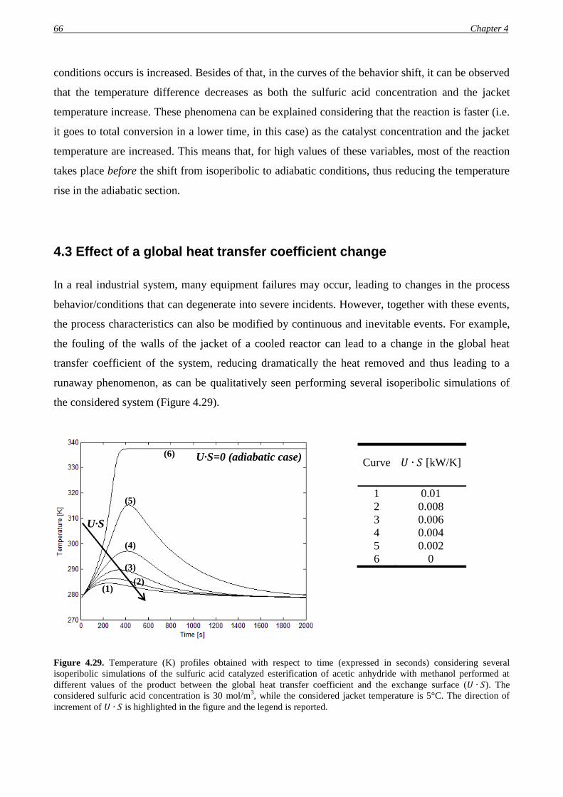
4.3 EFFECT OF A GLOBAL HEAT TRANSFER COEFFICIENT CHANGE…..…....66
CHAPTER 5 – Conclusions and observations……………..……………………....69
ANNEX………………..…………………………………..……………..…………..……….73
NOMENCLATURE AND SYMBOLS…………………………………..…...……….77
BIBLIOGRAPHIC REFERENCES………………………………………………..….81
Page 7
Introduction
Many of the incidents occurring in an industrial plant are due to the sudden release of a huge
amount of energy in a very short period of time and in a confined space. This typically
determines a sudden pressure increase, generating a shock wave that is violently propagated in
the surroundings, i.e. an explosion. It appears evident that these events must be avoided: this can
be done, for example, applying preventive measures that are based on the usage of different
criteria that are able to predict the thermal runaway of a system. The main objective of this thesis
is to apply and compare different runaway criteria and to develop a model that is able to detect
the boundaries between stable and unstable zone of the considered process.
In the first chapter, after a general description of the thermal behavior of a chemical process
(including the exposure of the general mass and energy balances), several runaway criteria are
presented and discussed from both a qualitative and a mathematical point of view.
In the second chapter, a brief description of reaction calorimetry (i.e. the main technique used to
obtain the experimental data required for this work) is followed by a specific description of the
experimental apparatus used to retrieve the data and by several considerations on the process that
is chosen to apply the runaway criteria. Then, the safety issues concerning the chemicals that are
taken into account are exposed.
In chapter three, a kinetic model of the system is developed and validated through the usage of
the retrieved experimental data. Then, the considered runaway criteria are applied to both
experimental and model data and the results are compared between each other.
In the fourth chapter, several adiabatic simulations of the system are performed in order to
simulate a dramatic failure of the cooling system in a real industrial reactor. Finally, a sensitivity
analysis of the maximum temperature reachable by the system is performed with respect to the
global heat transfer coefficient: this is done to simulate the effect of events such as the fouling of
the walls of the heat exchange system.
The fifth and last chapter is dedicated to the conclusions and to the final observations.
Page 9
Chapter 1
Background
Many industrial activities deal with transport, storage or transformation of chemicals. These
substances, because of their intrinsic properties, are often characterized by a high reactivity or a
flammable and/or explosive behavior, when specific conditions are met. Therefore, their use can
lead to incidents, endangering human beings and environment or, in the best scenario, simply
causing an economic damage to the company in which the incident occurs. Many of these events
are due to the sudden release of a huge amount of energy in a very short period of time and in a
confined space. This typically determines a sudden pressure increase, generating a shock wave
that is violently propagated in the surroundings, i.e. an explosion (1). It appears evident that these
events must be avoided: this can be done analyzing systematically all the potential hazards and
performing a risk analysis, trying to minimize the risk of incidents adopting both preventive and
protective measures. In this chapter, the focus is on the prevention of runaway (i.e. uncontrolled)
reactions, describing the theory of thermal explosion and several mathematical models that can
be adopted in order to foresee the occurrence of this kind of events, developing the so called
Early Warning Detection Systems (EWDS). Then, a brief description of the main calorimetric
techniques used in order to retrieve the information required to apply the above mentioned
criteria is presented.
1.1 Runaway reactions
It is well known that an increase of temperature leads to an exponential increase in the kinetic
constants of elementary reactions, thus causing, in most cases, an acceleration of the kinetics of
the global reaction. Therefore, if the thermal control in a reacting system subject to the
production of heat is lost, a runaway reaction may occur. This phenomenon is also called thermal
explosion and it also implies the possibility of the occurrence of side decomposition reactions
that can lead to the formation of volatile substances and, independently by this, the increase in
pressure in the vessel in which the process is carried out.
Page 10
4 Chapter 1
This type of event is characterized by an incremental increase of heat generation that, at a certain
point, determines the overheating of the reacting mass due to the fact that the heat production
rate becomes greater than the heat lost or exchanged by an eventual cooling system. In this way,
the thermal control of the process is lost and the pressure usually increases because of the vapor
pressure of the chemicals or the formation of gaseous by-products. A runaway reaction (or
thermal explosion) can occur either because the rate of heat generation is greater than the rate of
heat removal or because of chained-branched processes: the former cause leads to a proper
thermal runaway, while the latter one characterizes the so called “chain branching-induced
explosion”. In many events (e.g. in combustions or oxidations), it is quite difficult to distinguish
between the two mechanisms.
There is not a unique cause for the occurrence of a runaway reaction. In fact, it can originate
because of an incorrect kinetic evaluation, an excessive feed rate of the reagents, the presence of
impurities in the reactor, an inadequate mixing of chemicals (leading to the so called hot spots)
or the failure of one between the cooling and the stirring system. Human error is one of the major
causes of this kind of events (2).
It is well known that many industrial incidents are caused by runaway reactions (3): developing a
theory that is able to predict their occurrence is thus fundamental in order to introduce adequate
measures that can prevent them.
1.2 Thermal explosion theory
As it was previously said (§ 1.1), runaway reactions are essentially caused by the loss of the
thermal control in the system in which the process occurs. Therefore, the understanding of the
heat production and removal is essential to describe these phenomena. The theory of thermal
explosion concerns the causes of an explosion, the conditions of its occurrence and the prediction
of the temperature distribution in the reacting mass during the steady state and of the temperature
profile during the transient. It appears evident that the instruments related to this approach have
an enormous importance in the safety and risk prevention field (4).
The approaches for the description of runaway phenomena that can be found in literature can be
essentially classified as geometry or sensitivity based. In the former, the thermal explosion is
described according to some geometrical features of the system; on the other hand, the latter are
related to the parametric sensitivity of the system and are very suitable for practical applications.
Page 11
Background 5
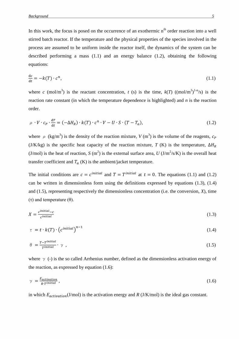
In this work, the focus is posed on the occurrence of an exothermic nth
order reaction into a well
stirred batch reactor. If the temperature and the physical properties of the species involved in the
process are assumed to be uniform inside the reactor itself, the dynamics of the system can be
described performing a mass (1.1) and an energy balance (1.2), obtaining the following
equations:
d𝑐
d𝑡= −𝑘(𝑇) ∙ 𝑐𝑛, (1.1)
where c (mol/m3) is the reactant concentration, t (s) is the time, k(T) ((mol/m
3)1-n
/s) is the
reaction rate constant (in which the temperature dependence is highlighted) and n is the reaction
order.
ρ ∙ 𝑉 ∙ 𝑐𝑃 ∙d𝑇
d𝑡= (−∆𝐻𝑅) ∙ 𝑘(𝑇) ∙ 𝑐𝑛 ∙ 𝑉 − 𝑈 ∙ 𝑆 ∙ (𝑇 − 𝑇𝑎), (1.2)
where ρ (kg/m3) is the density of the reaction mixture, V (m
3) is the volume of the reagents, 𝑐𝑃
(J/K/kg) is the specific heat capacity of the reaction mixture, T (K) is the temperature, ∆𝐻𝑅
(J/mol) is the heat of reaction, S (m2) is the external surface area, U (J/m
2/s/K) is the overall heat
transfer coefficient and 𝑇𝑎 (K) is the ambient/jacket temperature.
The initial conditions are 𝑐 = 𝑐𝑖𝑛𝑖𝑡𝑖𝑎𝑙 and 𝑇 = 𝑇𝑖𝑛𝑖𝑡𝑖𝑎𝑙 at 𝑡 = 0. The equations (1.1) and (1.2)
can be written in dimensionless form using the definitions expressed by equations (1.3), (1.4)
and (1.5), representing respectively the dimensionless concentration (i.e. the conversion, X), time
(τ) and temperature (θ).
𝑋 =𝑐𝑖𝑛𝑖𝑡𝑖𝑎𝑙−𝑐
𝑐𝑖𝑛𝑖𝑡𝑖𝑎𝑙 (1.3)
τ = 𝑡 ∙ 𝑘(𝑇) ∙ (𝑐𝑖𝑛𝑖𝑡𝑖𝑎𝑙)𝑛−1
(1.4)
θ =𝑇−𝑇𝑖𝑛𝑖𝑡𝑖𝑎𝑙
𝑇𝑖𝑛𝑖𝑡𝑖𝑎𝑙 ∙γ , (1.5)
where γ (-) is the so called Arrhenius number, defined as the dimensionless activation energy of
the reaction, as expressed by equation (1.6):
γ =𝐸𝑎𝑐𝑡𝑖𝑣𝑎𝑡𝑖𝑜𝑛
𝑅∙𝑇𝑖𝑛𝑖𝑡𝑖𝑎𝑙 , (1.6)
in which 𝐸𝑎𝑐𝑡𝑖𝑣𝑎𝑡𝑖𝑜𝑛(J/mol) is the activation energy and R (J/K/mol) is the ideal gas constant.
Page 12
6 Chapter 1
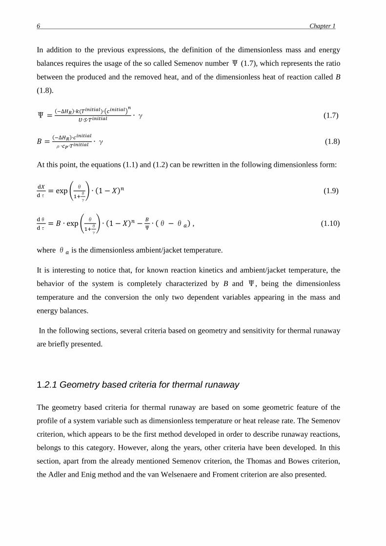
In addition to the previous expressions, the definition of the dimensionless mass and energy
balances requires the usage of the so called Semenov number Ψ (1.7), which represents the ratio
between the produced and the removed heat, and of the dimensionless heat of reaction called B
(1.8).
Ψ =(−∆𝐻𝑅)∙𝑘(𝑇𝑖𝑛𝑖𝑡𝑖𝑎𝑙)∙(𝑐𝑖𝑛𝑖𝑡𝑖𝑎𝑙)
𝑛
𝑈∙𝑆∙𝑇𝑖𝑛𝑖𝑡𝑖𝑎𝑙∙γ (1.7)
𝐵 =(−∆𝐻𝑅)∙𝑐𝑖𝑛𝑖𝑡𝑖𝑎𝑙
ρ∙𝑐𝑃∙𝑇𝑖𝑛𝑖𝑡𝑖𝑎𝑙 ∙γ (1.8)
At this point, the equations (1.1) and (1.2) can be rewritten in the following dimensionless form:
d𝑋
dτ= exp (
θ
1+θ
γ
) ∙ (1 − 𝑋)𝑛 (1.9)
dθ
dτ= 𝐵 ∙ exp (
θ
1+θ
γ
) ∙ (1 − 𝑋)𝑛 −𝐵
Ψ∙ (θ−θ𝑎) , (1.10)
where θ𝑎 is the dimensionless ambient/jacket temperature.
It is interesting to notice that, for known reaction kinetics and ambient/jacket temperature, the
behavior of the system is completely characterized by B and Ψ, being the dimensionless
temperature and the conversion the only two dependent variables appearing in the mass and
energy balances.
In the following sections, several criteria based on geometry and sensitivity for thermal runaway
are briefly presented.
1.2.1 Geometry based criteria for thermal runaway
The geometry based criteria for thermal runaway are based on some geometric feature of the
profile of a system variable such as dimensionless temperature or heat release rate. The Semenov
criterion, which appears to be the first method developed in order to describe runaway reactions,
belongs to this category. However, along the years, other criteria have been developed. In this
section, apart from the already mentioned Semenov criterion, the Thomas and Bowes criterion,
the Adler and Enig method and the van Welsenaere and Froment criterion are also presented.
Page 13
Background 7
1.2.1.1 The Semenov criterion
The Semenov criterion was developed in the 1928 (5). Semenov theory works well for gas and
liquid phase and small particle suspended systems that undergo self-heating in a turbulent regime
(as happens in well stirred reactors). It is important to observe that this method is based on the
assumption of negligible reactant consumption, which is obviously violated in most real systems.
However, its simplicity and explicitness allow one to have a fundamentally correct and synthetic
view of the mechanism of thermal explosion phenomena. In addition to this, Semenov theory is a
good approximation for a number of real systems, describing quite well the behavior of highly
reactive processes, in which the thermal explosions occur at very low values of conversion.
When reactant consumption is neglected (i.e. the conversion X tends to zero), the mass balance
equation (1.9) can be eliminated, while the energy balance (1.10) reduces to equation (1.11).
dθ
dτ= 𝐵 ∙ exp (
θ
1+θ
γ
) −𝐵
Ψ∙ (θ−θ𝑎) , (1.11)
Defining the rate of temperature increase due to the heat released by an eventual reaction as
θ+ = exp (θ
1+θ/γ) and the rate of temperature decrease due to heat removed by cooling as
θ− =1
Ψ∙ (θ−θ𝑎) , equation (1.11) can be rearranged in the following way:
1
𝐵∙
dθ
dτ=θ+ −θ− (1.12)
It can be demonstrated that the dynamic behavior of the system is fully determined by the
Semenov number Ψ. In particular, there are two critical values of Ψ, defining three different
operational characteristics of the system:
If Ψ >Ψ𝑐 , the system undergoes thermal runaway;
If Ψ𝑐′ <Ψ <Ψ𝑐 , the reaction can operate at a low temperature steady state but
runaway is possible for large perturbations in temperature;
If Ψ <Ψ𝑐′ , the system becomes intrinsically stable in operation temperature.
The critical Semenov numbers Ψ𝑐′ and Ψ𝑐 can be easily found by imposing a tangency
condition to the θ+ vs θ and θ− vs θ curves, finding, in this way, the critical values of the
dimensionless temperature that, being substituted in equation (1.11), allows to obtain the values
of Ψ𝑐′ and Ψ𝑐 . Considering only the condition over which the system undergoes thermal
Page 14
8 Chapter 1
runaway, the following expressions for the critical temperature θ𝑐 (1.13) and for the critical
Semenov number Ψ𝑐 (1.14) are obtained:
θ𝑐 =γ
2∙ [(γ− 2) − √γ(γ− 4) − 4θ𝑎] (1.13)
Ψ𝑐 = (θ𝑐 −θ𝑎) ∙ exp (−θ𝑐
1+θ𝑐γ
) (1.14)
Although this criterion is simple to understand and explicit, it is surely too conservative when
reactant consumption cannot be neglected. For this reason, criteria such as the Thomas and
Bowes, the Adler and Enig and the van Welsenaere and Froment ones are also presented.
1.2.1.2 The Thomas and Bowes criterion
The Thomas and Bowes criterion (6) is based on physical intuition and proposes to identify
thermal runaway as the situation in which a positive second-order derivative appears before the
dimensionless temperature maximum in the θ-τ plane. In fact, if the θ vs τ curve becomes
concave prior to reaching its maximum, the temperature increase results to be accelerated, even
if the curve returns to be convex as it approaches the maximum value itself. However, it can be
observed that the concave region enlarges as the Semenov number increases. Therefore, Thomas
and Bowes identified the critical condition for thermal runaway as the situation in which the
concave region first appears but its size is zero, i.e. when the two inflection points are coincident.
Formally speaking, this corresponds to the following conditions (1.15):
d2θ
dτ2 = 0 d3θ
dτ3 = 0 (1.15)
However, the equation (1.15) defines only the critical inflection point but it does not indicate
whether it is before or after the temperature maximum. Thus, with this criterion, it is generally
required to use some specific techniques to identify the inflection point that is before the
maximum. There exist several numerical strategies in the literature using equation (1.15) to find
the critical conditions for runaway, such as the ones proposed by Hlavacek et al. (7) or by
Morbidelli and Varma (8).
Page 15
Background 9
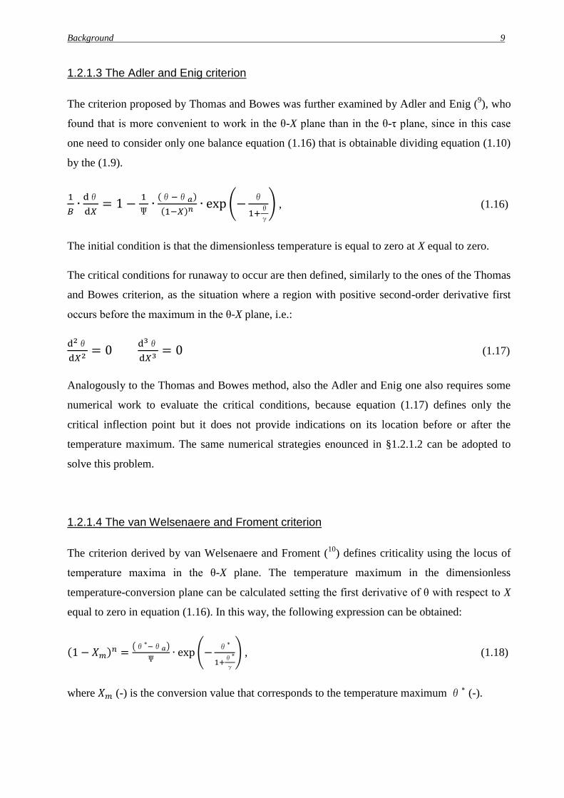
1.2.1.3 The Adler and Enig criterion
The criterion proposed by Thomas and Bowes was further examined by Adler and Enig (9), who
found that is more convenient to work in the θ-X plane than in the θ-τ plane, since in this case
one need to consider only one balance equation (1.16) that is obtainable dividing equation (1.10)
by the (1.9).
1
𝐵∙
dθ
d𝑋= 1 −
1
Ψ∙
(θ−θ𝑎)
(1−𝑋)𝑛∙ exp (−
θ
1+θ
γ
) , (1.16)
The initial condition is that the dimensionless temperature is equal to zero at X equal to zero.
The critical conditions for runaway to occur are then defined, similarly to the ones of the Thomas
and Bowes criterion, as the situation where a region with positive second-order derivative first
occurs before the maximum in the θ-X plane, i.e.:
d2θ
d𝑋2= 0
d3θ
d𝑋3= 0 (1.17)
Analogously to the Thomas and Bowes method, also the Adler and Enig one also requires some
numerical work to evaluate the critical conditions, because equation (1.17) defines only the
critical inflection point but it does not provide indications on its location before or after the
temperature maximum. The same numerical strategies enounced in §1.2.1.2 can be adopted to
solve this problem.
1.2.1.4 The van Welsenaere and Froment criterion
The criterion derived by van Welsenaere and Froment (10
) defines criticality using the locus of
temperature maxima in the θ-X plane. The temperature maximum in the dimensionless
temperature-conversion plane can be calculated setting the first derivative of θ with respect to X
equal to zero in equation (1.16). In this way, the following expression can be obtained:
(1 − 𝑋𝑚)𝑛 =(θ∗−θ𝑎)
Ψ∙ exp (−
θ∗
1+θ∗
γ
) , (1.18)
where 𝑋𝑚 (-) is the conversion value that corresponds to the temperature maximum θ∗ (-).
Page 16
10 Chapter 1
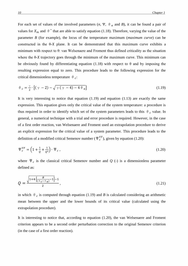
For each set of values of the involved parameters (n, Ψ, θ𝑎 and B), it can be found a pair of
values for 𝑋𝑚 and θ∗ that are able to satisfy equation (1.18). Therefore, varying the value of the
parameter B (for example), the locus of the temperature maximum (maximum curve) can be
constructed in the θ-X plane. It can be demonstrated that this maximum curve exhibits a
minimum with respect to θ: van Welsenaere and Froment thus defined criticality as the situation
where the θ-X trajectory goes through the minimum of the maximum curve. This minimum can
be obviously found by differentiating equation (1.18) with respect to θ and by imposing the
resulting expression equal to zero. This procedure leads to the following expression for the
critical dimensionless temperature θ𝑐:
θ𝑐 =γ
2∙ [(γ− 2) − √γ(γ− 4) − 4θ𝑎] (1.19)
It is very interesting to notice that equation (1.19) and equation (1.13) are exactly the same
expression. This equation gives only the critical value of the system temperature: a procedure is
thus required in order to identify which set of the system parameters leads to this θ𝑐 value. In
general, a numerical technique with a trial and error procedure is required. However, in the case
of a first order reaction, van Welsenaere and Froment used an extrapolation procedure to derive
an explicit expression for the critical value of a system parameter. This procedure leads to the
definition of a modified critical Semenov number (Ψ𝑐𝑉𝐹
), given by equation (1.20):
Ψ𝑐𝑉𝐹 = (1 +
1
𝑄+
1
𝑄2) ∙Ψ𝑐 , (1.20)
where Ψ𝑐 is the classical critical Semenov number and Q (-) is a dimensionless parameter
defined as:
𝑄 =√1+4∙[
𝐵
(θ𝑐−θ𝑎)−1]−1
2 , (1.21)
in which θ𝑐 is computed through equation (1.19) and B is calculated considering an arithmetic
mean between the upper and the lower bounds of its critical value (calculated using the
extrapolation procedure).
It is interesting to notice that, according to equation (1.20), the van Welsenaere and Froment
criterion appears to be a second order perturbation correction to the original Semenov criterion
(in the case of a first order reaction).
Page 17
Background 11
Considering the geometry based criteria for thermal runaway, it appears quite evident that they
can be applied only in systems where a temperature profile exists: this is certainly one of the
limitations of this kind of methods. Besides of that, they are not able to provide quantitative
measures of the extent or intensity of the runaway.
1.2.2 Sensitivity based criteria for thermal runaway
The geometry based criteria can be applied only to systems where a temperature profile exists,
which is not always the case in applications. Furthermore, they are not able to provide
indications on the intensity of the runaway, thus limiting the efficiency of an eventual action
taken to prevent the occurrence of a major incident caused by a thermal explosion, in a practical
application. For these reasons, a new series of criteria have been developed, based on the concept
of parametric sensitivity. These methods take advantage of the fact that, close to the boundary
between the runaway and non-runaway behavior, the system becomes very sensitive, i.e. its
behavior changes dramatically even if the initial values of the system parameters are subject to
very small perturbations: identifying this parametrically sensitive region thus allows to define
the critical conditions for thermal runaway.
In the following sections, the Hub and Jones, the Morbidelli and Varma and the Strozzi and
Zaldívar criteria are presented.
1.2.2.1 The Hub and Jones criterion
The Hub and Jones criterion (11
) states that the critical condition for runaway occurs when the
first derivative with respect to time of the temperature difference between the reactor and the
jacket is positive and, simultaneously to the previous condition, the second derivative of the
reactor temperature (even in this case, with respect to time) becomes equal to zero, i.e.:
d2𝑇
d𝑡2= 0
d(𝑇−𝑇𝑎)
d𝑡> 0 (1.22)
This criterion simply comes from the differentiation of the energy balance. In fact, computing
the time derivative of equation (1.2), the following one is obtained:
ρ ∙ 𝑉 ∙ 𝑐𝑃 ∙d2𝑇
dt2 =d[(−∆𝐻𝑅)∙𝑘(𝑇)∙𝑐𝑛∙𝑉]
d𝑡− 𝑈 ∙ 𝑆 ∙
d(𝑇−𝑇𝑎)
d𝑡 , (1.23)
Page 18
12 Chapter 1
in which it can be easily seen that the accumulation of heat in the system becomes ever
increasing when both the derivatives that appear in equation (1.22) are positive.
In order to apply this method, only the measured values of the reactor and of the jacket
temperature are required to be known. This criterion, differently from the geometry-based ones,
does not need a model for the reaction, thus being suitable for the on-line application. However,
in practice, the main problem in its usage is the amplification of the noise in the temperature
signals due to differentiation. Therefore, in order to avoid false alarms, the application of digital
philters or algorithms for data smoothing is required.
1.2.2.2 The Morbidelli and Varma criterion
The Morbidelli and Varma criterion (4,8,12,13
) is focused on the recognition of the parametrically
sensitive region of the system: its aim is to mark, in this way, the boundary for thermal
explosion. In order to do this, it is necessary to study the effect of the variation of some
parameter on the system behavior: this is done using the tools provided by the sensitivity
analysis.
The local sensitivity (s), with respect to a generic parameter Φ𝑖 , of a system whose behavior is
described by a single variable x (and its change in time is defined by the equation d𝑥/dt=f, with
𝑥(0) = 𝑥𝑖𝑛𝑖𝑡𝑖𝑎𝑙, where f (x, Φ, t) is continuous and differentiable in all its domain and where Φ
is a vector containing all the parameters of the system) is defined in the following way:
𝑠 =𝜕𝑥(𝑡,Φ𝑖)
𝜕Φ𝑖 (1.24)
The normalized sensitivity (𝑠𝑛𝑜𝑟𝑚) of x with respect to the parameter Φ𝑖 is used to normalize the
magnitudes of the parameter and of the system variable. It is defined in the following way:
𝑠𝑛𝑜𝑟𝑚 =Φ𝑖
𝑥∙
𝜕𝑥(𝑡,Φ𝑖)
𝜕Φ𝑖 (1.25)
In order to study specific characteristics of the system (as required by the Morbidelli and Varma
criterion), it is necessary to define the objective function sensitivity (𝑠𝑜𝑏𝑗):
𝑠𝑜𝑏𝑗 =𝜕𝐼
𝜕Φ𝑖 , (1.26)
Page 19
Background 13
in which I is the objective function, that is continuous with respect to the Φ𝑖 parameter. Of
course, equation (1.26) can be normalized, obtaining the so called normalized objective function
sensitivity:
𝑠𝑛𝑜𝑟𝑚𝑜𝑏𝑗
=Φ𝑖
𝐼∙
𝜕𝐼
𝜕Φ𝑖=
𝜕 ln 𝐼
𝜕 lnΦ𝑖 (1.27)
The Morbidelli and Varma criterion utilizes the normalized objective function sensitivity,
considering the maximum dimensionless temperature θ∗ as objective function. It is based on the
fact that, close to the boundary for thermal runaway, the normalized sensitivity of the maximum
temperature reaches itself its maximum value. The condition of maximum sensitivity is thus
considered the critical condition for thermal runaway in this criterion.
The sign of the sensitivity has a meaning: if positive, it indicates that the temperature maximum
increases as the value of the chosen parameter increases (and vice versa), i.e. the thermal
explosion occurs when the value of the parameter increases (and vice versa).
It was demonstrated by Morbidelli and Varma (13
) that, when a system is in the parametrically
sensitive region, this criterion is intrinsic, i.e. it provides the same value of the critical Semenov
number for thermal runaway independently on the choice of the parameter considered in order to
compute the normalized maximum temperature sensitivity. On the other hand, if the critical
value is dependent on the choice of the parameter, then the system is said to be parametrically
insensitive. In this case, one cannot define a general boundary that indicates the transition
between non-runaway and runaway behavior, and each situation needs to be analyzed
individually according to specific characteristics desired (e.g. maximum temperature lower than
a fixed value).
Only when the normalized objective function sensitivity maximum is sharp and essentially
independent on the parameter choice, one is really dealing with a potentially explosive system.
In fact, the intensity of the maximum provides quantitative information on the extent of the
thermal explosion.
1.2.2.3 The Strozzi and Zaldívar criterion
The Strozzi and Zaldivar criterion is based on the chaos theory techniques (14
). Applying this
approach, a mathematical model is not required for the process, thus making this criterion
suitable for on-line application in the detection of runaway reactions.
Page 20
14 Chapter 1
For a chemical reaction occurring in a batch reactor, when 𝑡 → ∞, the trajectory of the system in
the phase space tends to a specific point (for example, that at which the temperature of the
reactor is equal to the ambient/jacket temperature and the reactant conversion is complete). In
other words, the trajectory of two points that, at the beginning of the reaction, are close to each
other in the phase space, have to finish at the same final point when the reaction is complete.
However, the orbits of the two points can diverge along the path towards the final one and so, if
the system parameters are near the runaway boundary, a small initial position change results in a
large change in the phase space trajectories. Evaluating the divergence of the system of ordinary
differential equations that describes a chemical process (mass and energy balances), thus allows
to individuate the critical condition for thermal runaway. In particular, if, at a certain point of the
T vs t trajectory, a local positive divergence appears, the process operates in runaway conditions.
In the Strozzi and Zaldívar approach, the Lyapunov exponents are used to define sensitivity, and
so to quantify the rate of divergence of the above mentioned trajectories. It is well known that
the Lyapunov exponent can monitor the behavior of two neighboring points of a system in a
direction of the phase space, as function of time, classifying it depending on the exponent sign:
If the Laypunov exponent is positive, then the points diverge to each other;
If the exponent tends to zero, the points remain at the same relative distance;
If the exponent is negative, the points converge.
The on-line application of this criterion requires the reconstruction of the phase space of the
system by non-linear time series analysis using delay coordinate embedding (i.e. the usage of
time delays in the temperature measurements). Then, it is required to study the evolution of the
divergence during the transient, considering that a positive divergence implies the presence of a
runaway behavior.
This method has been validated experimentally by different studies that demonstrated its
reliability for batch, semi-batch and continuous reactors operating in both isothermal (i.e. at
constant temperature of the reactor) and isoperibolic (i.e. at constant environment/jacket
temperature) conditions and with different types of reactions (chain reactions, equilibrium,
parallel and competing reactions) (15,16,17,18
).
Page 21
Background 15
1.3 Calorimetric techniques
In order to apply the criteria exposed in §1.2, it is fundamental to obtain several data related to
the heat production due to the presence of a reaction or to the heat exchanged by the system with
the environment/jacket. Besides of that, most of the methods that were previously presented
require the development of a model for the process to which they are applied. All of this
information can be retrieved using calorimetry, i.e. the science aimed at the measurement of heat
exchanged between a system and the surrounding environment during a chemical reaction or a
physical transformation. Although research in this field started in the latter part of the 18th
century and calorimetry techniques progressively improved in the 19th
century, this science has
gained more and more importance in the last years mainly because of its application to the risk
analysis field. In fact, it has proved to be very useful in order to evaluate the suitability of a
designed process, to avoid to work in conditions that can lead to unexpected side reactions and
decomposition of hazardous chemicals, to correctly size protection devices and to perform a
variety of engineering calculations.
There are four categories into which monitored parameters relevant to risk analysis can be
classified: temperature, pressure, heat or power and time. Temperature and heat are considered to
be indicators of the severity of the runaway reaction, even if pressure is the most relevant
parameter to control: in fact, it is mainly the sudden increase in pressure to cause damage to
equipment, harm to operators and undesired release of chemicals into the environment. In
general, it can be stated that the higher the temperature, the rate of heat release and pressure, the
higher is the risk of incidents. However, it must not be forgot that, especially in the incident
prevention field, the time scale over which the event takes place is fundamental. All of the above
mentioned information, as previously stated, can be retrieved applying calorimetric techniques
(19
).
The experimental devices used in calorimetry can be classified on the basis of several criteria,
such as the following ones:
- The reaction volume. If it is lower than one milliliter, the calorimeters are called
microcalorimeters (such as the ones concerning Differential Scanning Calorimetry DSC
and Differential Thermal Analysis DTA). If it is between one millimeter and 0.1 liters, the
calorimeters are called minicalorimeters (such as the Calvet or Thian calorimeter and the
Thermal Screening Unit TSU, which is presented in Figure 1.1). If the volume is between
0.3 and 10 liters, the apparatuses are called reaction calorimeters (19, 20
).
Page 22
16 Chapter 1
- The operating mode. With respect to this criterion, in fact, calorimeters can be classified
as isothermal, adiabatic, isoperibolic and oscillating temperature ones.
- The control system, distinguishing between the so called active and passive calorimeters.
- The construction (single or double calorimeters).
- The working principle. There are, for example, differential calorimeters, combustion
ones, etc.
Figure 1.1. A Thermal Screening Unit (TSU) by HEL. The indication of the main parts of the apparatus is reported
in the figure.
The application of different calorimetric techniques is fundamental in order to retrieve the
experimental data required to build an Early Warning Detection System. In this work, an
isoperibolic reaction calorimeter is used for this purpose.
Page 23
Chapter 2
Experimental apparatus and reaction
description
In order to compare the thermal runaway criteria presented in §1, it has been decided to consider
the sulfuric acid catalyzed esterification of acetic anhydride and methanol. This appears to be a
relatively safe reaction for studying thermal runaway in laboratory and, because of the modest
reaction enthalpy and low activation energy, this reaction provides a severe test for the runaway
criteria. In order to retrieve the experimental data required for the application of the runaway
criteria, an isoperibolic reaction calorimeter is used. In this chapter, after a brief description of
the main reaction calorimetry techniques, the experimental apparatus used in this work is
presented and several considerations on the esterification reaction are briefly exposed. In the last
sections, the safety risks concerning the usage of acetic anhydride and methanol are shortly
enunciated.
2.1 Reaction calorimetry
As stated in §1, reaction calorimetry concerns the usage of apparatuses that have a volume
greater than 0.3 liters but smaller than 10 liters. Reaction calorimetry is based on the resolution
of the energy balance for an agitated jacketed reactor, i.e.:
�̇�𝑎𝑐𝑐 = �̇�𝑐ℎ𝑒𝑚 + �̇�𝑒𝑥𝑐 + �̇�𝑙𝑜𝑠𝑠 + 𝑃𝑠𝑡𝑖𝑟𝑟𝑒𝑟 + �̇�𝑐, (2.1)
where �̇�𝑎𝑐𝑐 (W) is the accumulated heat flow, �̇�𝑐ℎ𝑒𝑚 (W) is the heat flow generated by the
reaction, �̇�𝑒𝑥𝑐 (W) is the heat flow exchanged by the jacket, �̇�𝑙𝑜𝑠𝑠 (W) is the heat flow dissipated
in the environment, 𝑃𝑠𝑡𝑖𝑟𝑟𝑒𝑟 (W) is the power developed in the mixing process and �̇�𝑐 (W) is the
compensation heat flow.
These terms can be expressed according to the following equations:
�̇�𝑎𝑐𝑐 = 𝐶𝑃𝑑𝑇
𝑑𝑡 (2.2)
�̇�𝑐ℎ𝑒𝑚 = 𝑟 ∙ 𝑉 ∙ (−∆𝐻𝑅) (2.3)
Page 24
18 Chapter 2
�̇�𝑒𝑥𝑐 = 𝑈 ∙ 𝑆 ∙ (𝑇𝑎 − 𝑇) (2.4)
𝑃𝑠𝑡𝑖𝑟𝑟𝑒𝑟 = 2 ∙ π ∙ 𝑀𝑑 ∙ 𝑁 (2.5)
in which 𝐶𝑃 (J/K) is the heat capacity of the reaction mixture, 𝑟 (mol/s/m3) is the reaction
velocity, 𝑀𝑑 (J) is the stirrer torque and 𝑁 (s-1
) is the agitator speed.
Depending on their operation mode, reaction calorimeters can be classified in isothermal,
isoperibolic and adiabatic ones. The corresponding energy balances can be obtained considering
one or more of the terms that appear in equation (2.1) equal to zero. In the following sections, the
main characteristics of each type of calorimeter are shortly exposed, together with some
considerations.
2.1.1 Isothermal calorimeters
The isothermal calorimeters allow to study the behavior of a sample at constant temperature,
making possible the determination of the parameters linked to the agitation efficiency and heat
exchange. Furthermore, this operation mode allows to determine the global heat exchange
coefficient and to obtain in a direct way the reaction velocity.
2.1.2 Isoperibolic calorimeters
Differently from the isothermal calorimeters, in the isoperibolic ones the jacket temperature is
maintained constant. This allows to obtain the same information of the isothermal calorimetry
without the need of a complex and expensive control system of the reactor temperature.
However, the global heat transfer coefficient between the jacket and the reactor (that can be
determined through a calibration performed using an heating element) must be high enough, in
order to guarantee the pseudo-isothermal conditions of the system. The main disadvantage of this
technique is the need of mathematical models in order to eliminate the effects of the reaction
temperature variations on the technical data. This limit is usually overcame regulating the
resistance between the inside of the reactor and the surroundings in a way that the maximum
temperature rise does not become higher than 2 °C.
Page 25
Experimental apparatus and reaction description 19
2.1.3 Adiabatic calorimeters
The adiabatic reaction calorimetry allows to obtain information on the safety of a chemical
process: the runaway phenomena, in fact, are very fast and therefore can be considered
approximatively adiabatic. Thus, a single experiment in adiabatic conditions can provide many
fundamental information useful for the design of chemical reactors and of storage tanks and can
become an important tool for the risk assessment in industrial plants. In particular, the adiabatic
calorimetry allows to determine several process parameters related to systems in which an
exothermic reaction occurs, such as the adiabatic temperature rise ∆𝑇𝑎𝑑 (K), the temperature and
pressure rise velocity, the global reaction rate and the conversion. The main advantage of this
technique is the simplicity of the required experimental apparatus: in order to work in adiabatic
conditions, in fact, a system must not exchange a significant amount of heat with the
environment (this means that no control system is required for the temperature). However,
mathematical models are required in order to decouple temperature and concentration effects in
the experimental profiles obtainable using this technique.
The adiabatic temperature rise, i.e. the maximum temperature increment observable in the
presence of an exothermic reaction that occurs in an adiabatic system, can be determined using
the following equation:
∆𝑇𝑎𝑑 =𝑚∙(−∆𝐻𝑅)
𝑀𝑐𝑃 , (2.6)
where 𝑚 (mol) is the initial number of moles of the reagents and 𝑀 is the mass of the reagents. It
appears quite evident that the determination of ∆𝑇𝑎𝑑 is affected by the thermic inertia of the
eventual sample holder (which can absorb part of the generated heat). This fact is usually taken
into account through the so called ϕ-factor (-):
ϕ =(∆𝑇𝑎𝑑)𝑡ℎ𝑒𝑜𝑟𝑒𝑡𝑖𝑐𝑎𝑙
(∆𝑇𝑎𝑑)𝑜𝑏𝑠𝑒𝑟𝑣𝑒𝑑=
𝑚𝑠𝑐𝑃𝑠+𝑚ℎ𝑐𝑃ℎ
𝑚𝑠𝑐𝑃𝑠= 1 +
𝑚ℎ𝑐𝑃ℎ
𝑚𝑠𝑐𝑃𝑠 , (2.7)
where 𝑚𝑠 and 𝑚ℎ (kg) are respectively the mass of the sample and of the sample order, while
𝑐𝑃𝑠 and 𝑐𝑃ℎ (J/K/kg) are the specific heat at constant pressure of the sample and the sample
holder itself. Of course, in order to obtain experimental data that are representative of the
adiabatic case, the ϕ-factor must be as close as possible to 1.
Page 26
20 Chapter 2
2.2 Experimental apparatus
In order to retrieve the experimental data required for the study of the thermal runaway in the
esterification of acetic anhydride and methanol, the isoperibolic calorimeter represented in
Figure 2.1 is used. The experimental apparatus is constituted by the following instruments:
Jacketed and stirred calorimeter (Buchi);
Control panel of the engine CYCLONE 075 BUCHIGLASUSTER, connected to the
personal computer;
Data acquisition cards National Instruments, connected to the personal computer;
Thermocriostat (Huber Tango), used to modify the temperature of the heating/cooling
fluid (silicon oil);
Personal computer, using which it is possible to control and acquire the experimental data
through a program.
Figure 2.1. The isoperibolic reaction calorimeter used in this work.
The stirred reactor is in hastelloy steel and it has a nominal volume of 250 milliliters: it can resist
up to 250 °C of temperature and 60 bar of internal pressure. For control purposes, data
acquisition and safety reasons, the following devices are installed on the top of the vessel:
Three platinum resistance thermometers (Pt100): one of them is dedicated to the
temperature control in the reaction ambient, while the other two are used to control the
temperature in the jacket;
Page 27
Experimental apparatus and reaction description 21
A pressure transducer used to measure the pressure in the reaction ambient;
A bursting disk;
A relief valve;
A valve for the introduction of the samples.
The set temperature of the jacket ranges from -2 to 20 °C. The experiments are performed by
adding acetic anhydride very quickly to a solution of sulfuric acid in methanol, both at the same
temperature as the jacket. In order to reach as near as possible the same temperature as the
methanol in the calorimeter, the stoppered conical flask filled with a weighted quantity of pure
acetic anhydride (99 % purity, on a weight basis) is placed in the bath of the thermostat for a
reasonable time.
Before the addition of acetic anhydride, however, a calibration of the instrument is performed.
When the calorimeter reaches the steady state (as indicated by an approximatively constant value
of the smoothed reactor temperature and small values of its rate of change), the determination of
the average value of the temperature of the reactor is started and continues for 10-15 minutes.
Then, the values of 𝑈 ∙ 𝑆 and 𝑐𝑃 are determined considering an average of the experimental
measurements performed imposing different temperatures inside the reactor. After the calibration
and the return of the calorimeter to a steady state, the flask of acetic anhydride is removed from
the thermostatic bath, its outside is wiped dry and the acetic anhydride is quickly poured inside
the calorimeter. After the completion of the reaction, a second calibration is made. However, the
values of 𝑈 ∙ 𝑆 and 𝑐𝑃 that are found in the two calibrations are very similar because of the small
quantity of acetic anhydride with respect to methanol.
2.3 Considerations on the involved reactions
The acid catalyzed esterification of acetic anhydride and methanol results in the production of
methyl acetate and acetic acid, as shown in equation (2.8):
Acetic Anhydride + Methanol → Methyl Acetate + Acetic Acid (2.8)
As it was previously mentioned, this exothermic reaction is relatively safe for studying thermal
runaway in the laboratory and provides a severe test for the runaway criteria.
Besides of this main reaction, a side esterification also appears, leading to the reaction between
methanol and acetic acid to give water and methyl acetate, as expressed by equation (2.9):
Page 28
22 Chapter 2
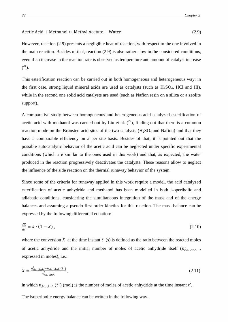
Acetic Acid + Methanol ↔ Methyl Acetate + Water (2.9)
However, reaction (2.9) presents a negligible heat of reaction, with respect to the one involved in
the main reaction. Besides of that, reaction (2.9) is also rather slow in the considered conditions,
even if an increase in the reaction rate is observed as temperature and amount of catalyst increase
(21
).
This esterification reaction can be carried out in both homogeneous and heterogeneous way: in
the first case, strong liquid mineral acids are used as catalysts (such as H2SO4, HCl and HI),
while in the second one solid acid catalysts are used (such as Nafion resin on a silica or a zeolite
support).
A comparative study between homogeneous and heterogeneous acid catalyzed esterification of
acetic acid with methanol was carried out by Liu et al. (22
), finding out that there is a common
reaction mode on the Brønsted acid sites of the two catalysts (H2SO4 and Nafion) and that they
have a comparable efficiency on a per site basis. Besides of that, it is pointed out that the
possible autocatalytic behavior of the acetic acid can be neglected under specific experimental
conditions (which are similar to the ones used in this work) and that, as expected, the water
produced in the reaction progressively deactivates the catalysts. These reasons allow to neglect
the influence of the side reaction on the thermal runaway behavior of the system.
Since some of the criteria for runaway applied in this work require a model, the acid catalyzed
esterification of acetic anhydride and methanol has been modelled in both isoperibolic and
adiabatic conditions, considering the simultaneous integration of the mass and of the energy
balances and assuming a pseudo-first order kinetics for this reaction. The mass balance can be
expressed by the following differential equation:
𝑑𝑋
𝑑𝑡= 𝑘 ∙ (1 − 𝑋) , (2.10)
where the conversion X at the time instant 𝑡′ (s) is defined as the ratio between the reacted moles
of acetic anhydride and the initial number of moles of acetic anhydride itself (𝑛𝐴𝑐. 𝐴𝑛ℎ.𝑖 ,
expressed in moles), i.e.:
𝑋 =𝑛𝐴𝑐. 𝐴𝑛ℎ.
𝑖 −𝑛𝐴𝑐. 𝐴𝑛ℎ.(𝑡′)
𝑛𝐴𝑐. 𝐴𝑛ℎ.𝑖 , (2.11)
in which 𝑛𝐴𝑐. 𝐴𝑛ℎ.(𝑡′) (mol) is the number of moles of acetic anhydride at the time instant 𝑡′.
The isoperibolic energy balance can be written in the following way.
Page 29
Experimental apparatus and reaction description 23
𝑚𝐴𝑐. 𝐴𝑛ℎ. ∙ 𝑐𝑃 ∙𝑑𝑇
𝑑𝑡= 𝑛𝐴𝑐. 𝐴𝑛ℎ.
𝑖 ∙ (−∆𝐻𝑅) ∙𝑑𝑋
𝑑𝑡− 𝑈 ∙ 𝑆 ∙ (𝑇 − 𝑇𝑎), (2.12)
in which 𝑚𝐴𝑐. 𝐴𝑛ℎ. (kg) is the mass of acetic anhydride inside the calorimeter.
In adiabatic conditions, equation (2.3) becomes:
𝑚𝐴𝑐. 𝐴𝑛ℎ. ∙ 𝑐𝑃 ∙𝑑𝑇
𝑑𝑡= 𝑛𝐴𝑐. 𝐴𝑛ℎ.
𝑖 ∙ (−∆𝐻𝑅) ∙𝑑𝑋
𝑑𝑡 (2.13)
By using an appropriate numeric technique in order to integrate simultaneously the mass and the
energy balances equations and by using the retrieved experimental data in order to obtain a
kinetic model of the esterification reaction and the values of 𝑐𝑃 and 𝑈 ∙ 𝑆, it is possible to obtain
a model for the reaction that allows the reconstruction of the T vs t curves parametrically with
respect to the sulfuric acid concentration and to the jacket temperature (which is approximatively
constant, in isoperibolic conditions).
2.4 Safety issues
It is well known that the chemicals involved in this reaction, i.e. acetic anhydride, methanol and
sulfuric acid, are dangerous for the human health and for the environment. However, in this case,
the sulfuric acid is used as a catalyst: the quantity involved in the reaction is thus small enough
to guarantee the absence of safety risks. On the other hand, acetic anhydride and methanol are
utilized in relevant quantities: in the following sections, the characteristics of these chemicals are
shortly presented, together with several examples of real incidents caused by these substances.
2.4.1 Acetic Anhydride
Acetic Anhydride, at ambient temperature, is a colorless liquid with a characteristic sharp odor.
It is used in making plastics, drugs, dyes, explosives, aspirin and perfumes. It is dangerous
because it is a highly corrosive chemical: its inhalation can irritate the mouth, the nose and the
throat, causing severe damage to the human body. Moreover, this chemical can be adsorbed
through the skin, causing irritations, skin allergies and severe damages to the eyes. Apart from
toxicity, acetic anhydride is also subject to flammability issues and can generate explosions. The
pictograms and the hazard/precautionary statements concerning this chemical are reported in
Figure 2.2.
Page 30
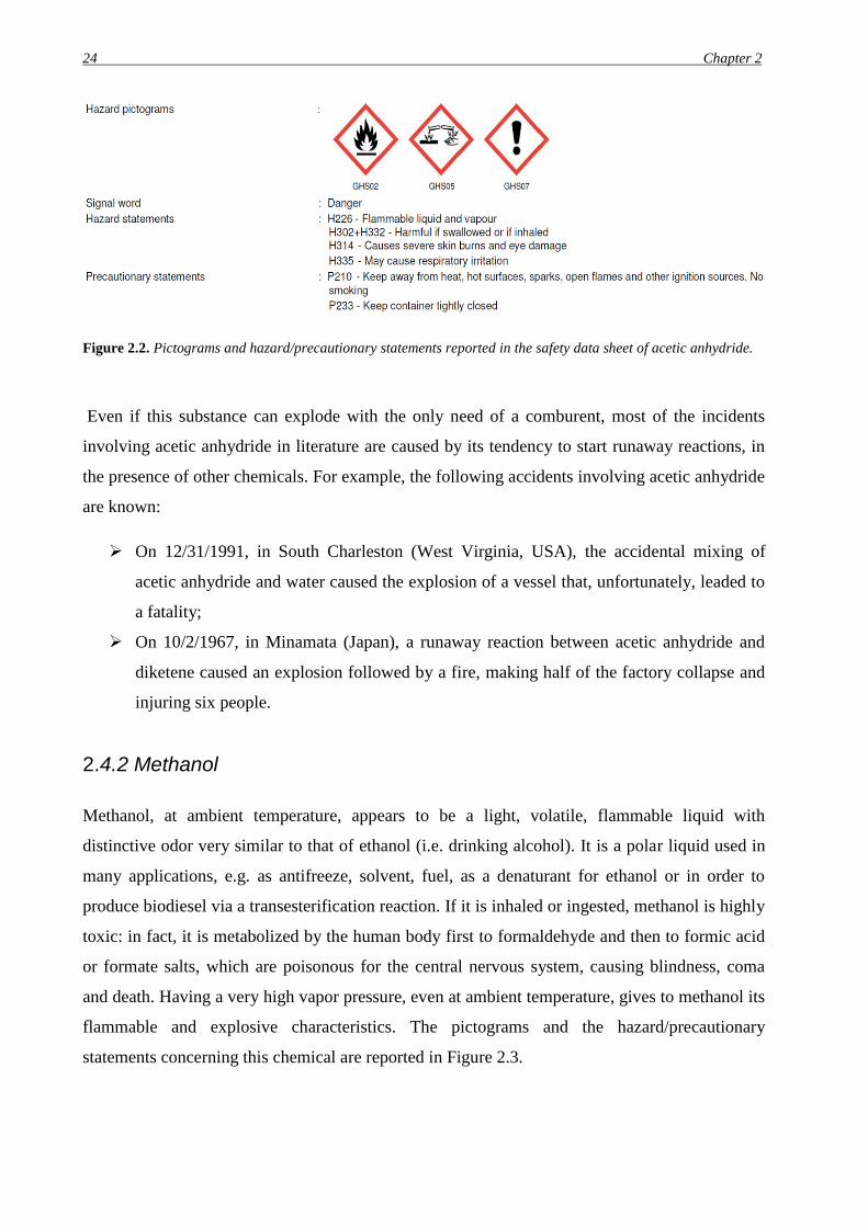
24 Chapter 2
Figure 2.2. Pictograms and hazard/precautionary statements reported in the safety data sheet of acetic anhydride.
Even if this substance can explode with the only need of a comburent, most of the incidents
involving acetic anhydride in literature are caused by its tendency to start runaway reactions, in
the presence of other chemicals. For example, the following accidents involving acetic anhydride
are known:
On 12/31/1991, in South Charleston (West Virginia, USA), the accidental mixing of
acetic anhydride and water caused the explosion of a vessel that, unfortunately, leaded to
a fatality;
On 10/2/1967, in Minamata (Japan), a runaway reaction between acetic anhydride and
diketene caused an explosion followed by a fire, making half of the factory collapse and
injuring six people.
2.4.2 Methanol
Methanol, at ambient temperature, appears to be a light, volatile, flammable liquid with
distinctive odor very similar to that of ethanol (i.e. drinking alcohol). It is a polar liquid used in
many applications, e.g. as antifreeze, solvent, fuel, as a denaturant for ethanol or in order to
produce biodiesel via a transesterification reaction. If it is inhaled or ingested, methanol is highly
toxic: in fact, it is metabolized by the human body first to formaldehyde and then to formic acid
or formate salts, which are poisonous for the central nervous system, causing blindness, coma
and death. Having a very high vapor pressure, even at ambient temperature, gives to methanol its
flammable and explosive characteristics. The pictograms and the hazard/precautionary
statements concerning this chemical are reported in Figure 2.3.
Page 31
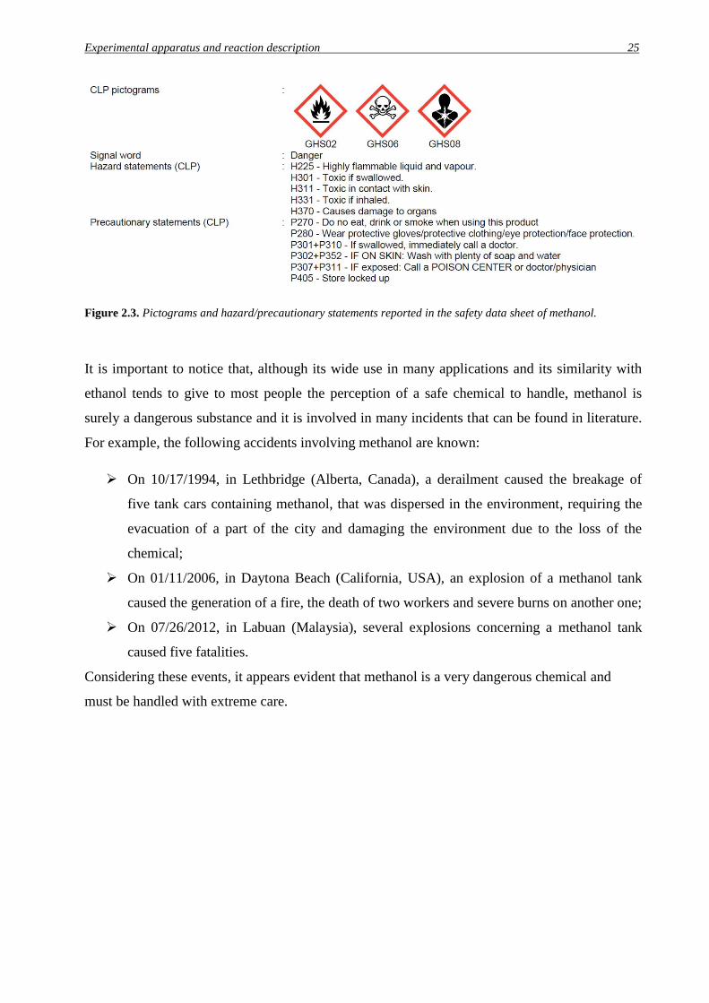
Experimental apparatus and reaction description 25
Figure 2.3. Pictograms and hazard/precautionary statements reported in the safety data sheet of methanol.
It is important to notice that, although its wide use in many applications and its similarity with
ethanol tends to give to most people the perception of a safe chemical to handle, methanol is
surely a dangerous substance and it is involved in many incidents that can be found in literature.
For example, the following accidents involving methanol are known:
On 10/17/1994, in Lethbridge (Alberta, Canada), a derailment caused the breakage of
five tank cars containing methanol, that was dispersed in the environment, requiring the
evacuation of a part of the city and damaging the environment due to the loss of the
chemical;
On 01/11/2006, in Daytona Beach (California, USA), an explosion of a methanol tank
caused the generation of a fire, the death of two workers and severe burns on another one;
On 07/26/2012, in Labuan (Malaysia), several explosions concerning a methanol tank
caused five fatalities.
Considering these events, it appears evident that methanol is a very dangerous chemical and
must be handled with extreme care.
Page 33
Chapter 3
Application of runaway criteria
(isoperibolic case)
In this chapter, the application of several criteria for the prediction of the thermal runaway to the
acid catalyzed esterification of acetic anhydride and methanol is presented. In particular, a
geometry-based criteria (Thomas and Bowes) and three sensitivity-based ones (Hub and Jones,
Morbidelli and Varma, Strozzi and Zaldìvar) are compared between each other, in order to
highlight the main differences and the possible limits of these methods, considering their
application in the isoperibolic case. As it was stated in §1, the Thomas and Bowes criterion and
the Morbidelli and Varma one require a model for the system, in order to be applied. In the
following sections, the development of this model is briefly presented, together with the results
of the application of the above mentioned runaway criteria and their comparison with the ones
presented by Casson et al. (17
).
3.1 Model of the acid catalyzed esterification
As it was stated in §2.1, a model for the acid catalyzed esterification of acetic anhydride and
methanol is constructed by the simultaneous integration of the mass and the isoperibolic energy
balances over time, considering a pseudo first order kinetics for the reaction. In order to build
this model, an isoperibolic calorimeter is used, performing several measurements (at different
concentration of sulfuric acid and jacket temperature) in order to retrieve the experimental curves
required for this operation. In each test, 0.8 mol of acetic anhydride and 7.0 mol of methanol are
used: the excess of methanol justifies the assumption of a pseudo-first order kinetics for the
reaction. The same experimental apparatus is used to obtain, through several calibrations, the
mean values of the system’s thermal capacity 𝑚𝐴𝑐. 𝐴𝑛ℎ. ∙ 𝑐𝑃 (i.e. 0.88 J/K) and of 𝑈 ∙ 𝑆 (i.e. 4.3
W/K).
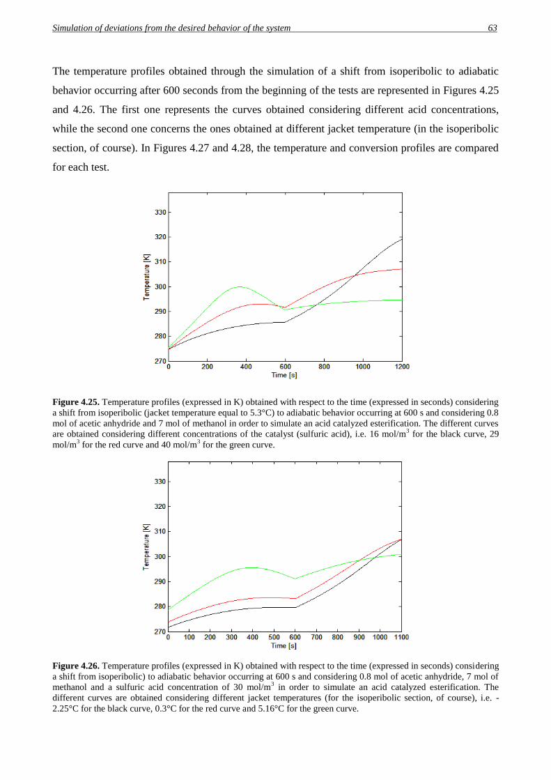
The experimental curves obtained considering an approximatively constant jacket temperature of
5.3 °C and different concentrations of sulfuric acid are represented in Figure 3.1, while the ones
obtained considering a sulfuric acid concentration of 30 mol/m3 and different jacket temperatures
are represented in Figure 3.2.
Page 34
28 Chapter 3
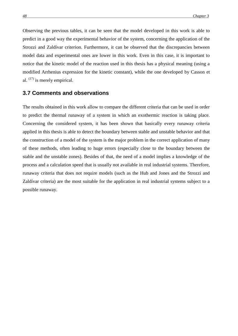
Figure 3.1. Temperature profiles (expressed in K) obtained with respect to the time (expressed in seconds) using a
calorimetric reactor in isoperibolic mode, maintaining an approximatively constant jacket temperature of 5.3 °C and
using 0.8 mol of acetic anhydride and 7 mol of methanol in order to carry out an acid catalyzed esterification. The
different curves are obtained using different concentrations of the catalyst (sulfuric acid), i.e. 16 mol/m3 for curve
(A), 29 mol/m3 for curve (B), 40 mol/m
3 for curve (C), 45 mol/m
3 for curve (D), 52 mol/m
3 for curve (E), 81 mol/m
3
for curve (F) and 100 mol/m3 for curve (G).
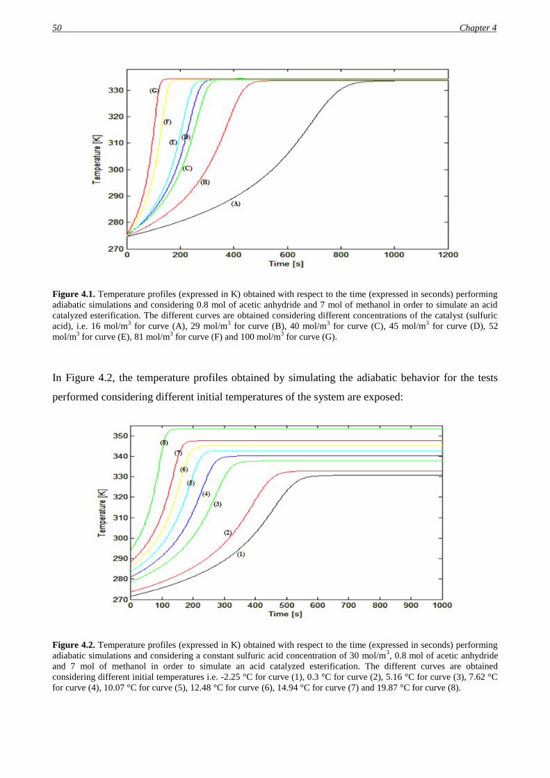
Figure 3.2. Temperature profiles (expressed in K) obtained with respect to the time (expressed in seconds) using a
calorimetric reactor in isoperibolic mode, using 0.8 mol of acetic anhydride,7 mol of methanol and a concentration
of 30 mol/m3 of sulfuric acid in order to carry out an acid catalyzed esterification. The different curves are obtained
at different jacket temperatures, i.e. -2.25 °C for curve (1), 0.3 °C for curve (2), 5.16 °C for curve (3), 7.62 °C for
curve (4), 10.07 °C for curve (5), 12.48 °C for curve (6), 14.94 °C for curve (7) and 19.87 °C for curve (8).
In order to obtain an expression for the kinetic constant of the esterification reaction, thus
building a model for the considered process, the mass and the isoperibolic energy balances are
integrated using a fourth order Runge-Kutta method and using a MATLAB®
script (that is
reported in the compact disk attached to this thesis and briefly described in the Annex) to
Page 35
Application of runaway criteria (isoperibolic case) 29
perform a minimization of the squared errors between the model and the experimental data, thus
obtaining the values of the parameters appearing in the kinetic constant. The expression of the
kinetic constant which was chosen to this purpose is the modified Arrhenius one, in order to give
a strong theoretical basis to the model and to take into account the temperature dependence of
the pre-exponential term. The effect of the catalyst concentration is taken into account
considering a linear dependence of the kinetic constant value from it. These procedures leaded to
the following expression:
𝑘 = 164.68 ∙ 𝑇1.0554 ∙ [𝐻2𝑆𝑂4] ∙ 𝑒−5932.8/𝑇, (3.1)
where [𝐻2𝑆𝑂4] is the sulfuric acid concentration expressed in mol/m3 and the temperature is
expressed in kelvin.
The comparison between the model predictions and the experimental data is represented in the
following figures (Figure 3.3, 3.4, 3.5 and 3.6).
Figure 3.3. Comparison between model predictions and experimental data for the experiments carried out using an
approximatively constant jacket temperature of 5.3 °C and different sulfuric acid concentrations, i.e. 16 mol/m3 for
test (A), 29 mol/m3 for test (B), 40 mol/m
3 for test (C) and 45 mol/m
3 for test (D). The green lines are referred to the
experimental data, while the red lines are the model predictions.
Page 36
30 Chapter 3
Figure 3.4. Comparison between model predictions and experimental data for the experiments carried out using an
approximatively constant jacket temperature of 5.3 °C and different sulfuric acid concentrations, i.e. 52 mol/m3 for
test (E), 81 mol/m3 for test (F) and 100 mol/m
3 for test (G). The green lines are referred to the experimental data,
while the red lines are the model predictions.
Figure 3.5. Comparison between model predictions and experimental data for the experiments carried out using a
sulfuric acid concentration of 30 mol/m3 and different jacket temperatures, i.e. -2.25 °C for curve (1), 0.3 °C for
curve (2), 5.16 °C for curve (3) and 7.62 °C for curve (4). The green lines are referred to the experimental data,
while the red lines are the model predictions.
Page 37
Application of runaway criteria (isoperibolic case) 31
Figure 3.6. Comparison between model predictions and experimental data for the experiments carried out using a
sulfuric acid concentration of 30 mol/m3 and different jacket temperatures, i.e. 10.07 °C for curve (5), 12.48 °C for
curve (6), 14.94 °C for curve (7) and 19.87 °C for curve (8). The green lines are referred to the experimental data,
while the red lines are the model predictions.
As it can be seen from the previous figures, the developed model seems to predict with a
sufficient degree of precision the behavior of the system represented by the experimental data. In
the following sections, the runaway criteria mentioned at the beginning of this chapter are
applied to both experimental and model data, in order to evaluate quantitatively the accuracy of
the model predictions and the differences between the considered criteria.
3.2 Hub and Jones criterion
In order to apply the Hub and Jones criterion, the second derivative of temperature with respect
to time is computed for both experimental and model data, in order to find out its maximum
value and thus finding out where approximatively is the boundary of the runaway behavior for
the considered system. The derivatives are computed numerically as incremental ratios; however,
the noise, which is inevitably present in the experimental data, required the application of a
filtering technique in order to avoid its amplification in the derivatives calculations. Therefore, a
third order Savitzky-Golay filter with a frame length of five experimental points was applied in
order to smooth the data without losing information. These calculations are performed using the
Page 38
32 Chapter 3
MATLAB® scripts that are reported in the compact disk attached to this thesis and briefly
described in the Annex.
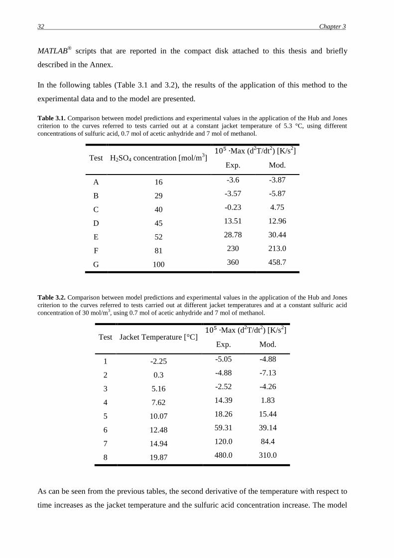
In the following tables (Table 3.1 and 3.2), the results of the application of this method to the
experimental data and to the model are presented.
Table 3.1. Comparison between model predictions and experimental values in the application of the Hub and Jones
criterion to the curves referred to tests carried out at a constant jacket temperature of 5.3 °C, using different
concentrations of sulfuric acid, 0.7 mol of acetic anhydride and 7 mol of methanol.
Test H2SO4 concentration [mol/m3]
105 ∙Max (d2T/dt
2) [K/s
2]
Exp. Mod.
A 16 -3.6 -3.87
B 29 -3.57 -5.87
C 40 -0.23 4.75
D 45 13.51 12.96
E 52 28.78 30.44
F 81 230 213.0
G 100 360 458.7
Table 3.2. Comparison between model predictions and experimental values in the application of the Hub and Jones
criterion to the curves referred to tests carried out at different jacket temperatures and at a constant sulfuric acid
concentration of 30 mol/m3, using 0.7 mol of acetic anhydride and 7 mol of methanol.
Test Jacket Temperature [°C] 105 ∙Max (d
2T/dt
2) [K/s
2]
Exp. Mod.
1 -2.25 -5.05 -4.88
2 0.3 -4.88 -7.13
3 5.16 -2.52 -4.26
4 7.62 14.39 1.83
5 10.07 18.26 15.44
6 12.48 59.31 39.14
7 14.94 120.0 84.4
8 19.87 480.0 310.0
As can be seen from the previous tables, the second derivative of the temperature with respect to
time increases as the jacket temperature and the sulfuric acid concentration increase. The model
Page 39
Application of runaway criteria (isoperibolic case) 33
seems to predict in a good way the real behavior of the system; however, the error increases
close to the boundary between stable and unstable behavior because of the great sensitivity of the
system in this zone.
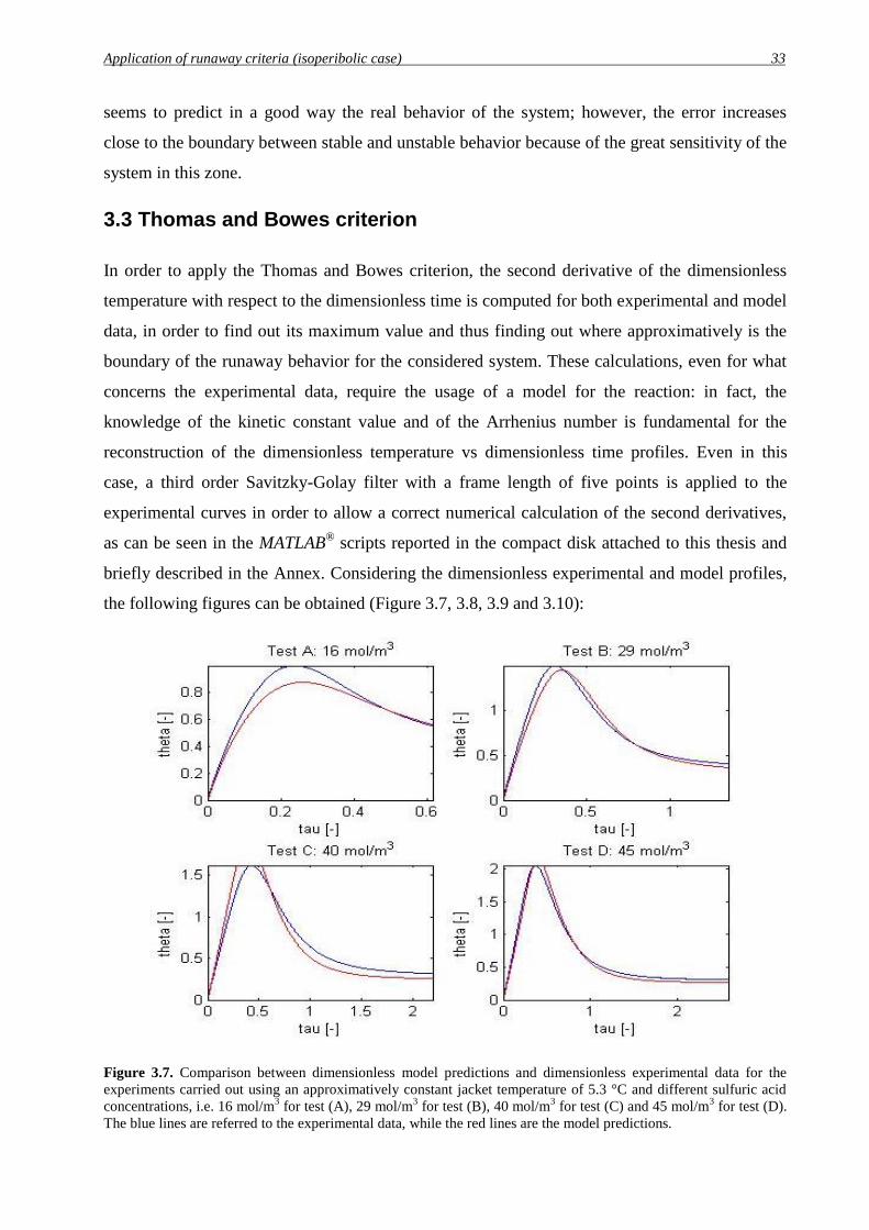
3.3 Thomas and Bowes criterion
In order to apply the Thomas and Bowes criterion, the second derivative of the dimensionless
temperature with respect to the dimensionless time is computed for both experimental and model
data, in order to find out its maximum value and thus finding out where approximatively is the
boundary of the runaway behavior for the considered system. These calculations, even for what
concerns the experimental data, require the usage of a model for the reaction: in fact, the
knowledge of the kinetic constant value and of the Arrhenius number is fundamental for the
reconstruction of the dimensionless temperature vs dimensionless time profiles. Even in this
case, a third order Savitzky-Golay filter with a frame length of five points is applied to the
experimental curves in order to allow a correct numerical calculation of the second derivatives,
as can be seen in the MATLAB® scripts reported in the compact disk attached to this thesis and
briefly described in the Annex. Considering the dimensionless experimental and model profiles,
the following figures can be obtained (Figure 3.7, 3.8, 3.9 and 3.10):
Figure 3.7. Comparison between dimensionless model predictions and dimensionless experimental data for the
experiments carried out using an approximatively constant jacket temperature of 5.3 °C and different sulfuric acid
concentrations, i.e. 16 mol/m3 for test (A), 29 mol/m
3 for test (B), 40 mol/m
3 for test (C) and 45 mol/m
3 for test (D).
The blue lines are referred to the experimental data, while the red lines are the model predictions.
Page 40
34 Chapter 3
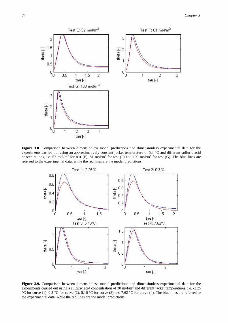
Figure 3.8. Comparison between dimensionless model predictions and dimensionless experimental data for the
experiments carried out using an approximatively constant jacket temperature of 5.3 °C and different sulfuric acid
concentrations, i.e. 52 mol/m3 for test (E), 81 mol/m
3 for test (F) and 100 mol/m
3 for test (G). The blue lines are
referred to the experimental data, while the red lines are the model predictions.
Figure 3.9. Comparison between dimensionless model predictions and dimensionless experimental data for the
experiments carried out using a sulfuric acid concentration of 30 mol/m3 and different jacket temperatures, i.e. -2.25
°C for curve (1), 0.3 °C for curve (2), 5.16 °C for curve (3) and 7.62 °C for curve (4). The blue lines are referred to
the experimental data, while the red lines are the model predictions.
Page 41
Application of runaway criteria (isoperibolic case) 35
Figure 3.10. Comparison between dimensionless model predictions and dimensionless experimental data for the
experiments carried out using a sulfuric acid concentration of 30 mol/m3 and different jacket temperatures, i.e. 10.07
°C for curve (5), 12.48 °C for curve (6), 14.94 °C for curve (7) and 19.87 °C for curve (8). The blue lines are
referred to the experimental data, while the red lines are the model predictions.
As it can be seen from the previous figures, the developed model seems to predict with a
sufficient degree of precision the behavior of the system represented by the experimental data.
However, in the absence of runaway phenomena, there are higher discrepancies between
experimental data and model predictions. In the following tables (Table 3.3 and 3.4), the results
of the application of the Thomas and Bowes method to the experimental data and to the model
are presented.
Table 3.3. Comparison between model predictions and experimental values in the application of the Thomas and
Bowes criterion to the curves referred to tests carried out at a constant jacket temperature of 5.3 °C, using different
concentrations of sulfuric acid, 0.7 mol of acetic anhydride and 7 mol of methanol.
Test H2SO4 concentration [mol/m3]
Max (d2θ/dτ
2) [-]
Exp. Mod.
A 16 -17.3 -17.7
B 29 -5.04 -8.63
C 40 -0.15 3.25
D 45 7.36 7.03
E 52 12.26 13.21
F 81 39.73 36.43
G 100 38.97 49.25
Page 42
36 Chapter 3
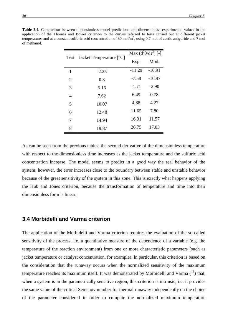
Table 3.4. Comparison between dimensionless model predictions and dimensionless experimental values in the
application of the Thomas and Bowes criterion to the curves referred to tests carried out at different jacket
temperatures and at a constant sulfuric acid concentration of 30 mol/m3, using 0.7 mol of acetic anhydride and 7 mol
of methanol.
Test Jacket Temperature [°C] Max (d
2θ/dτ
2) [-]
Exp. Mod.
1 -2.25 -11.29 -10.91
2 0.3 -7.58 -10.97
3 5.16 -1.71 -2.90
4 7.62 6.49 0.78
5 10.07 4.88 4.27
6 12.48 11.65 7.80
7 14.94 16.31 11.57
8 19.87 26.75 17.03
As can be seen from the previous tables, the second derivative of the dimensionless temperature
with respect to the dimensionless time increases as the jacket temperature and the sulfuric acid
concentration increase. The model seems to predict in a good way the real behavior of the
system; however, the error increases close to the boundary between stable and unstable behavior
because of the great sensitivity of the system in this zone. This is exactly what happens applying
the Hub and Jones criterion, because the transformation of temperature and time into their
dimensionless form is linear.
3.4 Morbidelli and Varma criterion
The application of the Morbidelli and Varma criterion requires the evaluation of the so called
sensitivity of the process, i.e. a quantitative measure of the dependence of a variable (e.g. the
temperature of the reaction environment) from one or more characteristic parameters (such as
jacket temperature or catalyst concentration, for example). In particular, this criterion is based on
the consideration that the runaway occurs when the normalized sensitivity of the maximum
temperature reaches its maximum itself. It was demonstrated by Morbidelli and Varma (13
) that,
when a system is in the parametrically sensitive region, this criterion is intrinsic, i.e. it provides
the same value of the critical Semenov number for thermal runaway independently on the choice
of the parameter considered in order to compute the normalized maximum temperature
Page 43
Application of runaway criteria (isoperibolic case) 37
sensitivity. For this reason, in this section, the normalized sensitivity is analyzed with respect to
the jacket temperature and to the sulfuric acid concentration. In order to apply this criterion to
the experimental data, the maximum temperature is collected for each experimental run and is
expressed in function of the considered characteristic parameter of the process through the usage
of a four parameters sigmoid fitting function. In this way, the local and the normalized
sensitivities are computed analytically. The Morbidelli and Varma criterion is also applied to the
model data, computing in a numeric way the sensitivities after the application of a third order
Savitzsky-Golay filter to smooth the small oscillations given by the model itself. These
calculations are performed using several MATLAB®
that are reported in the compact disk
attached to this thesis and briefly described in the Annex.
3.4.1 Sensitivity with respect to the jacket temperature
In this case, the local sensitivity of the system is defined in the following way:
𝑠 =𝜕𝑇𝑚𝑎𝑥
𝜕𝑇𝑎 , (3.2)
where 𝑇𝑚𝑎𝑥 (K) is the locus of the temperature maxima for the experimental runs carried out
varying the jacket temperature 𝑇𝑎 (K). The normalized sensitivity is thus defined according to the
following equation:
𝑠𝑛𝑜𝑟𝑚 =𝑇𝑎
𝑇𝑚𝑎𝑥∙
𝜕𝑇𝑚𝑎𝑥
𝜕𝑇𝑎 (3.3)
As it was previously stated, a four parameters sigmoid is used to fit the experimental data,
minimizing the errors between the fitting function and the experimental points and thus finding
the optimal values of the sigmoid parameters. This procedure leads to the following function:
𝑇𝑚𝑎𝑥 = 270.4892 +86.5375
1+𝑒[−
(𝑇𝑎−284.8807)7.4721
] (3.4)
In the following figure (Figure 3.11), the comparison between fitting function and experimental
data is shown.
Page 44
38 Chapter 3
Figure 3.11. Comparison between sigmoidal fitting function (green curve) and maximum temperatures experimental
points (blue) for the experiments carried out using a sulfuric acid concentration of 30 mol/m3 and different jacket
temperatures. The temperatures are expressed in kelvin.
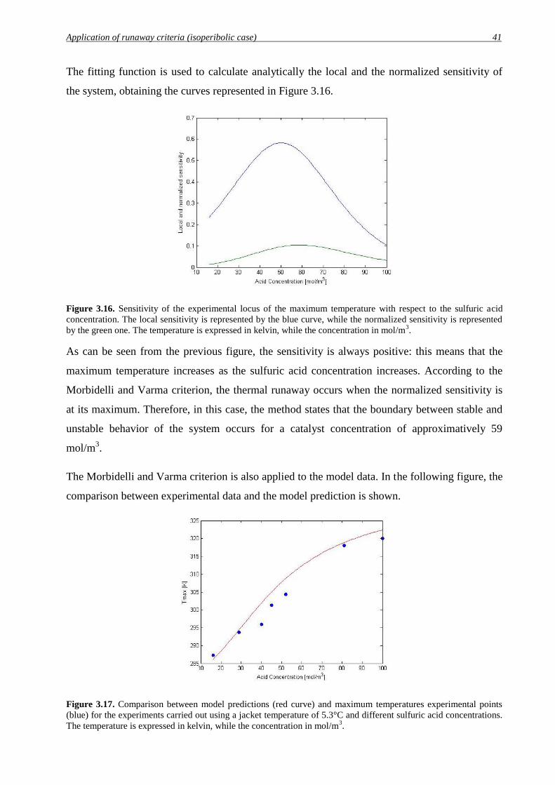
The fitting function is used to calculate analytically the local and the normalized sensitivity of
the system, obtaining the curves represented in Figure 3.12.
Figure 3.12. Sensitivity of the experimental locus of the maximum temperature with respect to the jacket
temperature. The local sensitivity is represented by the blue curve, while the normalized sensitivity is represented by
the green one. The temperatures are expressed in kelvin.
As can be seen from the previous figure, the sensitivity is always positive: this means that the
maximum temperature increases as the jacket temperature increases. According to the Morbidelli
and Varma criterion, the thermal runaway occurs when the normalized sensitivity is at its
maximum. Therefore, in this case, the method states that the boundary between stable and
unstable behavior of the system is around a jacket temperature of 284.4 K.
Page 45
Application of runaway criteria (isoperibolic case) 39
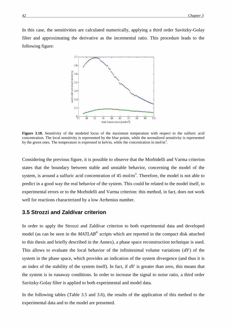
The Morbidelli and Varma criterion is also applied to the model data. In the following figure, the
comparison between the experimental data and the model prediction is shown.
Figure 3.13. Comparison between model predictions (red curve) and maximum temperatures experimental points
(blue) for the experiments carried out using a sulfuric acid concentration of 30 mol/m3 and different jacket
temperatures. The temperatures are expressed in kelvin.
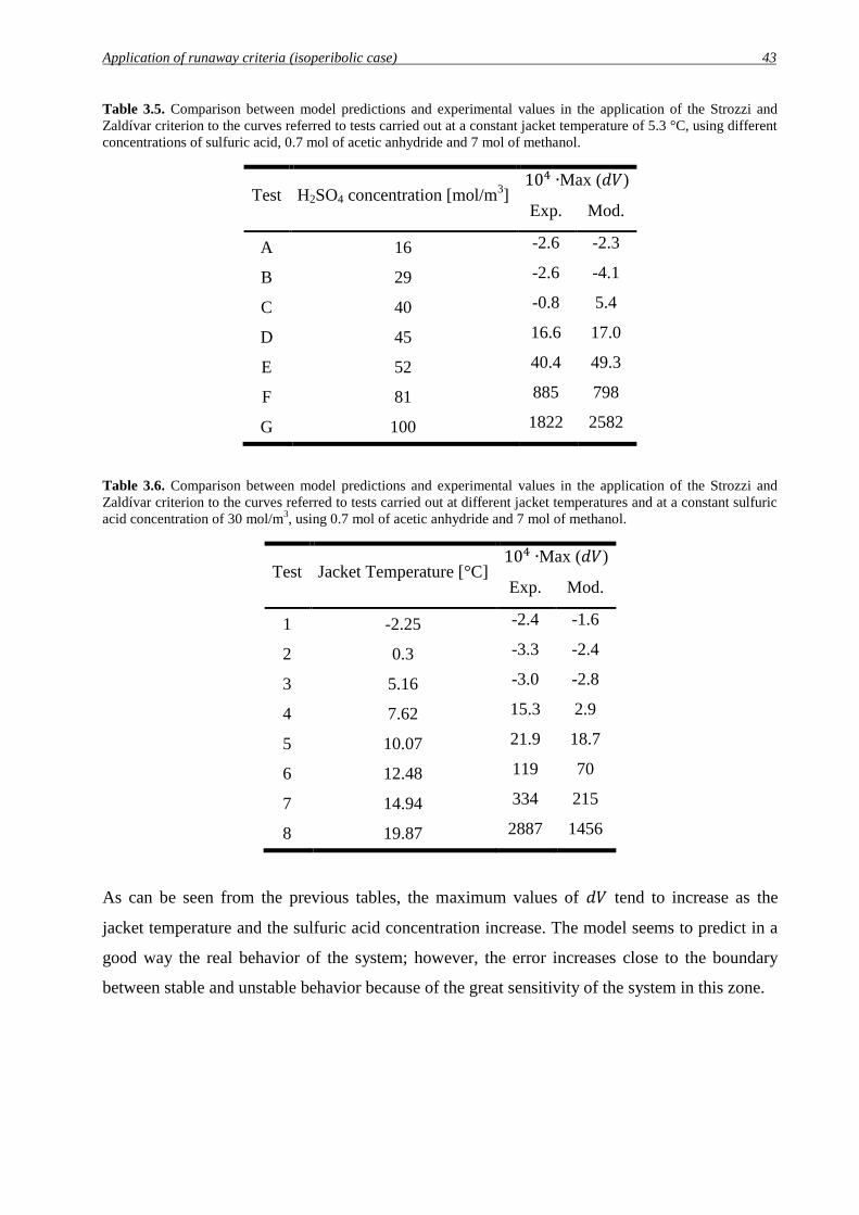
In this case, the sensitivities are calculated numerically, applying a Savitzky-Golay filter and
approximating the derivative as the incremental ratio. This procedure leads to the following
figure:
Figure 3.14. Sensitivity of the modelled locus of the maximum temperature with respect to the jacket temperature.
The local sensitivity is represented by the blue points, while the normalized sensitivity is represented by the green
ones. The temperatures are expressed in kelvin.
Considering the previous figure, it is possible to observe that the Morbidelli and Varma criterion
states that the boundary between stable and unstable behavior, concerning the model of the
system, is around a jacket temperature of 282 K. Therefore, the model is able to predict in a good
way the real behavior of the system.
Page 46
40 Chapter 3
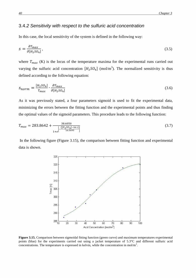
3.4.2 Sensitivity with respect to the sulfuric acid concentration
In this case, the local sensitivity of the system is defined in the following way:
𝑠 =𝜕𝑇𝑚𝑎𝑥
𝜕[𝐻2𝑆𝑂4] , (3.5)
where 𝑇𝑚𝑎𝑥 (K) is the locus of the temperature maxima for the experimental runs carried out
varying the sulfuric acid concentration [𝐻2𝑆𝑂4] (mol/m3). The normalized sensitivity is thus
defined according to the following equation:
𝑠𝑛𝑜𝑟𝑚 =[𝐻2𝑆𝑂4]
𝑇𝑚𝑎𝑥∙
𝜕𝑇𝑚𝑎𝑥
𝜕[𝐻2𝑆𝑂4] (3.6)
As it was previously stated, a four parameters sigmoid is used to fit the experimental data,
minimizing the errors between the fitting function and the experimental points and thus finding
the optimal values of the sigmoid parameters. This procedure leads to the following function:
𝑇𝑚𝑎𝑥 = 283.8642 +38.6050
1+𝑒[−
([𝐻2𝑆𝑂4]−50.1)
16.5695]
(3.7)
In the following figure (Figure 3.15), the comparison between fitting function and experimental
data is shown.
Figure 3.15. Comparison between sigmoidal fitting function (green curve) and maximum temperatures experimental
points (blue) for the experiments carried out using a jacket temperature of 5.3°C and different sulfuric acid
concentrations. The temperature is expressed in kelvin, while the concentration in mol/m3.
Page 47
Application of runaway criteria (isoperibolic case) 41
The fitting function is used to calculate analytically the local and the normalized sensitivity of
the system, obtaining the curves represented in Figure 3.16.
Figure 3.16. Sensitivity of the experimental locus of the maximum temperature with respect to the sulfuric acid
concentration. The local sensitivity is represented by the blue curve, while the normalized sensitivity is represented
by the green one. The temperature is expressed in kelvin, while the concentration in mol/m3.
As can be seen from the previous figure, the sensitivity is always positive: this means that the
maximum temperature increases as the sulfuric acid concentration increases. According to the
Morbidelli and Varma criterion, the thermal runaway occurs when the normalized sensitivity is
at its maximum. Therefore, in this case, the method states that the boundary between stable and
unstable behavior of the system occurs for a catalyst concentration of approximatively 59
mol/m3.
The Morbidelli and Varma criterion is also applied to the model data. In the following figure, the
comparison between experimental data and the model prediction is shown.
Figure 3.17. Comparison between model predictions (red curve) and maximum temperatures experimental points
(blue) for the experiments carried out using a jacket temperature of 5.3°C and different sulfuric acid concentrations.
The temperature is expressed in kelvin, while the concentration in mol/m3.
Page 48
42 Chapter 3
In this case, the sensitivities are calculated numerically, applying a third order Savitzky-Golay
filter and approximating the derivative as the incremental ratio. This procedure leads to the
following figure:
Figure 3.18. Sensitivity of the modeled locus of the maximum temperature with respect to the sulfuric acid
concentration. The local sensitivity is represented by the blue points, while the normalized sensitivity is represented
by the green ones. The temperature is expressed in kelvin, while the concentration in mol/m3.
Considering the previous figure, it is possible to observe that the Morbidelli and Varma criterion
states that the boundary between stable and unstable behavior, concerning the model of the
system, is around a sulfuric acid concentration of 45 mol/m3. Therefore, the model is not able to
predict in a good way the real behavior of the system. This could be related to the model itself, to
experimental errors or to the Morbidelli and Varma criterion: this method, in fact, does not work
well for reactions characterized by a low Arrhenius number.
3.5 Strozzi and Zaldívar criterion
In order to apply the Strozzi and Zaldívar criterion to both experimental data and developed
model (as can be seen in the MATLAB®
scripts which are reported in the compact disk attached
to this thesis and briefly described in the Annex), a phase space reconstruction technique is used.
This allows to evaluate the local behavior of the infinitesimal volume variations (𝑑𝑉) of the
system in the phase space, which provides an indication of the system divergence (and thus it is
an index of the stability of the system itself). In fact, if 𝑑𝑉 is greater than zero, this means that
the system is in runaway conditions. In order to increase the signal to noise ratio, a third order
Savitzky-Golay filter is applied to both experimental and model data.
In the following tables (Table 3.5 and 3.6), the results of the application of this method to the
experimental data and to the model are presented.
Page 49
Application of runaway criteria (isoperibolic case) 43
Table 3.5. Comparison between model predictions and experimental values in the application of the Strozzi and
Zaldívar criterion to the curves referred to tests carried out at a constant jacket temperature of 5.3 °C, using different
concentrations of sulfuric acid, 0.7 mol of acetic anhydride and 7 mol of methanol.
Test H2SO4 concentration [mol/m3]
104 ∙Max (𝑑𝑉)
Exp. Mod.
A 16 -2.6 -2.3
B 29 -2.6 -4.1
C 40 -0.8 5.4
D 45 16.6 17.0
E 52 40.4 49.3
F 81 885 798
G 100 1822 2582
Table 3.6. Comparison between model predictions and experimental values in the application of the Strozzi and
Zaldívar criterion to the curves referred to tests carried out at different jacket temperatures and at a constant sulfuric
acid concentration of 30 mol/m3, using 0.7 mol of acetic anhydride and 7 mol of methanol.
Test Jacket Temperature [°C] 104 ∙Max (𝑑𝑉)
Exp. Mod.
1 -2.25 -2.4 -1.6
2 0.3 -3.3 -2.4
3 5.16 -3.0 -2.8
4 7.62 15.3 2.9
5 10.07 21.9 18.7
6 12.48 119 70
7 14.94 334 215
8 19.87 2887 1456
As can be seen from the previous tables, the maximum values of 𝑑𝑉 tend to increase as the
jacket temperature and the sulfuric acid concentration increase. The model seems to predict in a
good way the real behavior of the system; however, the error increases close to the boundary
between stable and unstable behavior because of the great sensitivity of the system in this zone.
Page 50
44 Chapter 3
3.6 Comparison with the results obtained by Casson et al.
In order to have a further indication of the effectiveness of the model developed for the system,
the above exposed results are compared with the ones obtained in the scientific publication
“Comparison of criteria for prediction of runaway reactions in the sulfuric acid catalyzed
esterification of acetic anhydride and methanol” by Casson et al. (17
). The latter, in fact,
compared different runaway criteria using the same experimental apparatus utilized in this thesis
work; however, a different model was developed for the esterification reaction. In the following
sections, the results of the two works are reported, only considering the runaway criteria and the
experimental conditions that are common to the two works.
3.6.1 Comparison of results for the Hub and Jones criterion
In the following table (Table 3.7), the comparison between the results obtained in this work
applying the Hub and Jones criterion to the experimental runs at different sulfuric acid
concentration and the ones reported in the work by Casson et al. is exposed.
Table 3.7. Comparison between the results obtained applying the Hub and Jones criterion in this thesis work and in
the scientific publication by Casson et al. (17
). The tests are carried out at a constant jacket temperature of 5.3 °C,
using different concentrations of sulfuric acid, 0.7 mol of acetic anhydride and 7 mol of methanol. Both model and
experimental results are reported.
H2SO4 Concentration
[mol/m3]
105 ∙Max (d2T/dt
2)
[K/s2]
105 ∙Max (d2T/dt
2) Casson et al.
[K/s2]
Exp. Mod. Exp. Mod.
29 -3.57 -5.87 -6 -5
45 13.51 12.97 8 20
52 28.78 30.44 20 48
81 230 213 300 290
100 360 459 400 640
In the following table (Table 3.8), the comparison between the results obtained in this work
applying the Hub and Jones criterion to the experimental runs at different jacket temperature and
the ones reported in the work by Casson et al. is exposed.
Page 51
Application of runaway criteria (isoperibolic case) 45
Table 3.8. Comparison between the results obtained applying the Hub and Jones criterion in this thesis work and in
the scientific publication by Casson et al. (17
). The tests are carried out at different jacket temperature, using a
sulfuric acid concentration of 30 mol/m3, 0.7 mol of acetic anhydride and 7 mol of methanol. Both model and
experimental results are reported.
Jacket temperature [°C] 105 ∙Max (d
2T/dt
2) [K/s
2] 105 ∙Max (d
2T/dt
2) Casson et al. [K/s
2]
Exp. Mod. Exp. Mod.
5.16 -2.52 -4.26 -2 -5
10.07 18.26 15.44 6 10
12.48 59.31 39.14 30 44
14.94 120.0 84.40 93 100
19.87 480.0 310.0 300 260
Observing the previous tables, it can be seen that the model developed in this work is able to
predict in a good way the experimental behavior of the system, concerning the application of the
Hub and Jones criterion. Furthermore, it can be observed that the discrepancies between model
data and experimental ones obtained considering different concentrations of sulfuric acid are
lower in this work. Besides of that, it is important to say that the kinetic model of the reaction
described in §3.1 has a physical meaning; in contrast to this, the one developed in the scientific
publication of Casson et al. is merely empirical.
Page 52
46 Chapter 3
3.6.2 Comparison of results for the Thomas and Bowes criterion
In the following table (Table 3.9), the comparison between the results obtained in this work
applying the Thomas and Bowes criterion to the experimental runs at different sulfuric acid
concentration and the ones reported in the work by Casson et al. is exposed.
Table 3.9. Comparison between the results obtained applying the Thomas and Bowes criterion in this thesis work
and in the scientific publication by Casson et al. (17
). The tests are carried out at a constant jacket temperature of 5.3
°C, using different concentrations of sulfuric acid, 0.7 mol of acetic anhydride and 7 mol of methanol. Both model
and experimental results are reported.
H2SO4 Concentration [mol/m3]
Max (d2θ/dτ2
) [-] Max (d2θ/dτ2
) Casson et al. [-]
Exp. Mod. Exp. Mod.
16 -17.3 -17.7 -27 -27
29 -5.04 -8.63 -1 -7
45 7.36 7.03 5 11
52 12.26 13.21 8 20
81 39.73 36.43 30 50
100 38.97 49.25 32 73
In the following table (Table 3.10), the comparison between the results obtained in this work
applying the Thomas and Bowes criterion to the experimental runs at different jacket
temperature and the ones reported in the work by Casson et al. is exposed.
Table 3.10. Comparison between the results obtained applying the Thomas and Bowes criterion in this thesis work
and in the scientific publication by Casson et al. (17
). The tests are carried out at different jacket temperature, using a
sulfuric acid concentration of 30 mol/m3, 0.7 mol of acetic anhydride and 7 mol of methanol. Both model and
experimental results are reported.
Jacket temperature [°C] Max (d
2θ/dτ2) [-] Max (d
2θ/dτ2) Casson et al. [-]
Exp. Mod. Exp. Mod.
5.16 -1.71 -2.90 -1 -6
10.07 4.88 4.27 1 6
12.48 11.65 7.80 11 20
14.94 16.31 11.57 19 28
19.87 26.75 17.03 32 31
Observing the previous tables, it can be seen that the model developed in this work is able to
predict in a good way the experimental behavior of the system, concerning the application of the
Thomas and Bowes criterion. Furthermore, it can be observed that the discrepancies between
Page 53
Application of runaway criteria (isoperibolic case) 47
model data and experimental ones are lower in this work. Even in this case, it is important to
notice that the kinetic model of the reaction used in this thesis has a physical meaning, while the
one developed in the scientific publication of Casson et al. is merely empirical.
3.6.3 Comparison of results for the Strozzi and Zaldívar criterion
In the following tables (Table 3.11 and Table 3.12), the comparison between the results obtained
in this work applying the Strozzi and Zaldívar criterion and the ones reported in the scientific
publication by Casson et al. is exposed. The first one is referred to the data obtained considering
different sulfuric acid concentrations, while the second one is related to the consideration of
different jacket temperatures.
Table 3.11. Comparison between the results obtained applying the Strozzi and Zaldívar criterion in this thesis work
and in the scientific publication by Casson et al. (17
). The tests are carried out at a constant jacket temperature of 5.3
°C, using different concentrations of sulfuric acid, 0.7 mol of acetic anhydride and 7 mol of methanol. Both model
and experimental results are reported.
H2SO4 Concentration [mol/m3]
104 ∙Max (𝑑𝑉) 104 ∙Max (𝑑𝑉) Casson et al.
Exp. Mod. Exp. Mod.
29 -2.6 -4.1 -4 -5
45 16.6 17.0 20 40
52 40.4 49.3 40 100
81 885 798 840 1300
100 1822 2582 1700 2800
Table 3.12. Comparison between the results obtained applying the Strozzi and Zaldívar criterion in this thesis work
and in the scientific publication by Casson et al. (17
). The tests are carried out at different jacket temperature, using a
sulfuric acid concentration of 30 mol/m3, 0.7 mol of acetic anhydride and 7 mol of methanol. Both model and
experimental results are reported.
Jacket temperature [°C] 104 ∙Max (𝑑𝑉) 104 ∙Max (𝑑𝑉) Casson et al.
Exp. Mod. Exp. Mod.
5.16 -3.0 -2.8 -2 -5
10.07 21.9 18.7 5 110
12.48 119 70 73 120
14.94 334 215 230 370
19.87 2887 1456 1500 1200
Page 54
48 Chapter 3
Observing the previous tables, it can be seen that the model developed in this work is able to
predict in a good way the experimental behavior of the system, concerning the application of the
Strozzi and Zaldívar criterion. Furthermore, it can be observed that the discrepancies between
model data and experimental ones are lower in this work. Even in this case, it is important to
notice that the kinetic model of the reaction used in this thesis has a physical meaning (using a
modified Arrhenius expression for the kinetic constant), while the one developed by Casson et
al. (17)
is merely empirical.
3.7 Comments and observations
The results obtained in this work allow to compare the different criteria that can be used in order
to predict the thermal runaway of a system in which an exothermic reaction is taking place.
Concerning the considered system, it has been shown that basically every runaway criteria
applied in this thesis is able to detect the boundary between stable and unstable behavior and that
the construction of a model of the system is the major problem in the correct application of many
of these methods, often leading to huge errors (especially close to the boundary between the
stable and the unstable zones). Besides of that, the need of a model implies a knowledge of the
process and a calculation speed that is usually not available in real industrial systems. Therefore,
runaway criteria that does not require models (such as the Hub and Jones and the Strozzi and
Zaldívar criteria) are the most suitable for the application in real industrial systems subject to a
possible runaway.
Page 55
Chapter 4
Simulation of deviations from the desired
behavior of the system
Using the model of the acid catalyzed esterification reaction developed in §3.1, it is also possible to
perform adiabatic simulations of the reactive system behavior. This is very important because the
adiabatic conditions are the most dangerous ones: when a system cannot exchange heat with its
surroundings and an exothermic reaction is occurring, the self-heating rate and the temperature rise
reach their maximum values. The usage of the previously developed model thus allows to simulate
a sudden failure of the cooling system, e.g. the shift of the system behavior from isoperibolic to
adiabatic (worst conditions) or a change in the global heat transfer coefficient of the system itself.
In this chapter, after the presentation of the results obtained performing adiabatic simulations, the
case of the shift from isoperibolic to adiabatic behavior (at different time instants of the tests) is
analyzed. In the last section, the application of the Morbidelli and Varma criterion is exploited in
order to study the effect of a change in the global heat transfer coefficient on the system behavior.
4.1 Adiabatic simulations
As previously stated, the model developed in §3.1 allows to perform adiabatic simulations of the
sulfuric acid catalyzed esterification of acetic anhydride with methanol. With these data, it is also
possible to apply the runaway criteria exposed in §1; however, it appears quite obvious that an
adiabatic system in which occurs an exothermic reaction will surely become unstable. In Figure 4.1,
the temperature profiles obtained by simulating the adiabatic behavior for the tests performed
considering different concentrations of sulfuric acid are exposed. Observing it, it appears quite
evident that the system becomes more and more unstable as the concentration of sulfuric acid
increases. This qualitative observation is numerically confirmed by the application of the Hub and
Jones criterion. It is interesting to notice that the final temperature is the same for every test: this is
due to the facts that the simulations consider a complete conversion of the reagents and that the
amount of catalyst only affects the rate of the temperature rise but not the final value of the
temperature itself.
Page 56
50 Chapter 4
Figure 4.1. Temperature profiles (expressed in K) obtained with respect to the time (expressed in seconds) performing
adiabatic simulations and considering 0.8 mol of acetic anhydride and 7 mol of methanol in order to simulate an acid
catalyzed esterification. The different curves are obtained considering different concentrations of the catalyst (sulfuric
acid), i.e. 16 mol/m3 for curve (A), 29 mol/m
3 for curve (B), 40 mol/m
3 for curve (C), 45 mol/m
3 for curve (D), 52
mol/m3 for curve (E), 81 mol/m
3 for curve (F) and 100 mol/m
3 for curve (G).
In Figure 4.2, the temperature profiles obtained by simulating the adiabatic behavior for the tests
performed considering different initial temperatures of the system are exposed:
Figure 4.2. Temperature profiles (expressed in K) obtained with respect to the time (expressed in seconds) performing
adiabatic simulations and considering a constant sulfuric acid concentration of 30 mol/m3, 0.8 mol of acetic anhydride
and 7 mol of methanol in order to simulate an acid catalyzed esterification. The different curves are obtained
considering different initial temperatures i.e. -2.25 °C for curve (1), 0.3 °C for curve (2), 5.16 °C for curve (3), 7.62 °C
for curve (4), 10.07 °C for curve (5), 12.48 °C for curve (6), 14.94 °C for curve (7) and 19.87 °C for curve (8).
Page 57
Simulation of deviations from the desired behavior of the system 51
Observing the previous figure, it appears quite evident that the system becomes more and more
unstable as the initial temperature increases. This qualitative observation is numerically confirmed
by the application of the Hub and Jones criterion. It is interesting to notice that the final temperature
is different for each simulation, but the difference between the final and the initial temperature is
the same for everyone (adiabatic temperature rise).
The same tests are performed considering the dimensionless time and temperature, thus applying
the Thomas and Bowes criterion in order to verify the presence of a runaway behavior. In Figure
4.3, the dimensionless temperature profiles obtained by simulating the adiabatic behavior for the
tests performed considering different concentrations of sulfuric acid are exposed:
Figure 4.3. Dimensionless temperature profiles obtained with respect to the dimensionless time performing adiabatic
simulations and considering 0.8 mol of acetic anhydride and 7 mol of methanol in order to simulate an acid catalyzed
esterification. The different curves are obtained considering different concentrations of the catalyst (sulfuric acid), but
they appear to be approximatively coincident.
Observing the previous figure, it appears that the curves related to different catalyst concentration
are approximatively coincident, if plotted in dimensionless form. This is probably due to the fact
that the dimensionless time is computed using the initial value of the kinetic constant, whose
expression depends linearly on the sulfuric acid concentration. Of course, the coincidence of the
curves does not allow the Thomas and Bowes criterion to detect any difference between them (even
if the criterion is able to see that, in each case, the behavior of the system is unstable).
Page 58
52 Chapter 4
In Figure 4.4, the dimensionless temperature profiles obtained by simulating the adiabatic behavior
for the tests performed considering different initial temperatures are exposed:
Figure 4.4. Dimensionless temperature profiles obtained with respect to the dimensionless time performing adiabatic
simulations and considering a sulfuric acid concentration of 30 mol/m3, 0.8 mol of acetic anhydride and 7 mol of
methanol in order to simulate an acid catalyzed esterification. . The different curves are obtained at different initial
temperatures, i.e. -2.25 °C for curve (1), 0.3 °C for curve (2), 5.16 °C for curve (3), 7.62 °C for curve (4), 10.07 °C for
curve (5), 12.48 °C for curve (6), 14.94 °C for curve (7) and 19.87 °C for curve (8).
Observing the previous figure, it seems that the intensity of the runaway decreases as the initial
temperature increases. This is in contrast with the considerations exposed after the presentation of
Figure 4.2 and it is due to the definition of the dimensionless temperature (in which the initial
temperature appears at the denominator). Because of this, the Thomas and Bowes criterion cannot
be used to evaluate the intensity of the runaway in an adiabatic system: it can only be used to
discriminate between stable and unstable behavior.
4.2 Cooling system failure simulation
Using the model developed in §3.1, it is also possible to simulate many failures that can occur in an
industrial reactor. For instance, a sudden shift from isoperibolic to adiabatic behavior can be
simulated, considering, in this way, the worst possible failure conditions. The time at which this
shift occurs is very important: in order to study this effect, several simulations are carried out,
considering the tests that, in isoperibolic-only conditions, leaded to a stable behavior.
Page 59
Simulation of deviations from the desired behavior of the system 53
The temperature profiles obtained through the simulation of a shift from isoperibolic to adiabatic
behavior occurring after 100 seconds from the beginning of the tests are represented in Figures 4.5
and 4.6. The first one represents the curves obtained considering different acid concentrations,
while the second one concerns the ones obtained at different jacket temperature (in the isoperibolic
section, of course). In Figures 4.7 and 4.8, the temperature and conversion profiles are compared for
each test.
Figure 4.5. Temperature profiles (expressed in K) obtained with respect to the time (expressed in seconds) considering
a shift from isoperibolic (jacket temperature equal to 5.3°C) to adiabatic behavior occurring at 100 s and considering 0.8
mol of acetic anhydride and 7 mol of methanol in order to simulate an acid catalyzed esterification. The different curves
are obtained considering different concentrations of the catalyst (sulfuric acid), i.e. 16 mol/m3 for the black curve, 29
mol/m3 for the red curve and 40 mol/m
3 for the green curve.
Figure 4.6. Temperature profiles (expressed in K) obtained with respect to the time (expressed in seconds) considering
a shift from isoperibolic) to adiabatic behavior occurring at 100 s and considering 0.8 mol of acetic anhydride, 7 mol of
methanol and a sulfuric acid concentration of 30 mol/m3 in order to simulate an acid catalyzed esterification. The
different curves are obtained considering different jacket temperatures (for the isoperibolic section, of course), i.e. -
2.25°C for the black curve, 0.3°C for the red curve and 5.16°C for the green curve.
Page 60
54 Chapter 4
Figure 4.7. Temperature (expressed in K, red lines) and conversion (green lines) profiles obtained with respect to the
time (expressed in seconds) considering a shift from isoperibolic (jacket temperature equal to 5.3°C) to adiabatic
behavior occurring at 100 s and considering 0.8 mol of acetic anhydride and 7 mol of methanol in order to simulate an
acid catalyzed esterification. The different curves are obtained considering different concentrations of the catalyst
(sulfuric acid), i.e. 16 mol/m3 for the (A) curves, 29 mol/m
3 for the (B) curves and 40 mol/m
3 for the (C) curves.
Figure 4.8. Temperature (expressed in K, red lines) and conversion (green lines) profiles obtained with respect to the
time (expressed in seconds) considering a shift from isoperibolic) to adiabatic behavior occurring at 100 s and
considering 0.8 mol of acetic anhydride, 7 mol of methanol and a sulfuric acid concentration of 30 mol/m3 in order to
simulate an acid catalyzed esterification. The different curves are obtained considering different jacket temperatures (for
the isoperibolic section, of course), i.e. -2.25°C for the (A) curves, 0.3°C for the (B) curves and 5.16°C for the (C)
curves.
Page 61
Simulation of deviations from the desired behavior of the system 55
The temperature profiles obtained through the simulation of a shift from isoperibolic to adiabatic
behavior occurring after 200 seconds from the beginning of the tests are represented in Figures 4.9
and 4.10. The first one represents the curves obtained considering different acid concentrations,
while the second one concerns the ones obtained at different jacket temperature (in the isoperibolic
section, of course). In Figures 4.11 and 4.12, the temperature and conversion profiles are compared
for each test.
Figure 4.9. Temperature profiles (expressed in K) obtained with respect to the time (expressed in seconds) considering
a shift from isoperibolic (jacket temperature equal to 5.3°C) to adiabatic behavior occurring at 200 s and considering 0.8
mol of acetic anhydride and 7 mol of methanol in order to simulate an acid catalyzed esterification. The different curves
are obtained considering different concentrations of the catalyst (sulfuric acid), i.e. 16 mol/m3 for the black curve, 29
mol/m3 for the red curve and 40 mol/m
3 for the green curve.
Figure 4.10. Temperature profiles (expressed in K) obtained with respect to the time (expressed in seconds) considering
a shift from isoperibolic) to adiabatic behavior occurring at 200 s and considering 0.8 mol of acetic anhydride, 7 mol of
methanol and a sulfuric acid concentration of 30 mol/m3 in order to simulate an acid catalyzed esterification. The
different curves are obtained considering different jacket temperatures (for the isoperibolic section, of course), i.e. -
2.25°C for the black curve, 0.3°C for the red curve and 5.16°C for the green curve.
Page 62
56 Chapter 4
Figure 4.11. Temperature (expressed in K, red lines) and conversion (green lines) profiles obtained with respect to the
time (expressed in seconds) considering a shift from isoperibolic (jacket temperature equal to 5.3°C) to adiabatic
behavior occurring at 200 s and considering 0.8 mol of acetic anhydride and 7 mol of methanol in order to simulate an
acid catalyzed esterification. The different curves are obtained considering different concentrations of the catalyst
(sulfuric acid), i.e. 16 mol/m3 for the (A) curves, 29 mol/m
3 for the (B) curves and 40 mol/m
3 for the (C) curves.
Figure 4.12. Temperature (expressed in K, red lines) and conversion (green lines) profiles obtained with respect to the
time (expressed in seconds) considering a shift from isoperibolic) to adiabatic behavior occurring at 200 s and
considering 0.8 mol of acetic anhydride, 7 mol of methanol and a sulfuric acid concentration of 30 mol/m3 in order to
simulate an acid catalyzed esterification. The different curves are obtained considering different jacket temperatures (for
the isoperibolic section, of course), i.e. -2.25°C for the (A) curves, 0.3°C for the (B) curves and 5.16°C for the (C)
curves.
Page 63
Simulation of deviations from the desired behavior of the system 57
The temperature profiles obtained through the simulation of a shift from isoperibolic to adiabatic
behavior occurring after 300 seconds from the beginning of the tests are represented in Figures 4.13
and 4.14. The first one represents the curves obtained considering different acid concentrations,
while the second one concerns the ones obtained at different jacket temperature (in the isoperibolic
section, of course). In Figures 4.15 and 4.16, the temperature and conversion profiles are compared
for each test.
Figure 4.13. Temperature profiles (expressed in K) obtained with respect to the time (expressed in seconds) considering
a shift from isoperibolic (jacket temperature equal to 5.3°C) to adiabatic behavior occurring at 300 s and considering 0.8
mol of acetic anhydride and 7 mol of methanol in order to simulate an acid catalyzed esterification. The different curves
are obtained considering different concentrations of the catalyst (sulfuric acid), i.e. 16 mol/m3 for the black curve, 29
mol/m3 for the red curve and 40 mol/m
3 for the green curve.
Figure 4.14. Temperature profiles (expressed in K) obtained with respect to the time (expressed in seconds) considering
a shift from isoperibolic) to adiabatic behavior occurring at 300 s and considering 0.8 mol of acetic anhydride, 7 mol of
methanol and a sulfuric acid concentration of 30 mol/m3 in order to simulate an acid catalyzed esterification. The
different curves are obtained considering different jacket temperatures (for the isoperibolic section, of course), i.e. -
2.25°C for the black curve, 0.3°C for the red curve and 5.16°C for the green curve.
Page 64
58 Chapter 4
Figure 4.15. Temperature (expressed in K, red lines) and conversion (green lines) profiles obtained with respect to the
time (expressed in seconds) considering a shift from isoperibolic (jacket temperature equal to 5.3°C) to adiabatic
behavior occurring at 300 s and considering 0.8 mol of acetic anhydride and 7 mol of methanol in order to simulate an
acid catalyzed esterification. The different curves are obtained considering different concentrations of the catalyst
(sulfuric acid), i.e. 16 mol/m3 for the (A) curves, 29 mol/m
3 for the (B) curves and 40 mol/m
3 for the (C) curves.
Figure 4.16. Temperature (expressed in K, red lines) and conversion (green lines) profiles obtained with respect to the
time (expressed in seconds) considering a shift from isoperibolic) to adiabatic behavior occurring at 300 s and
considering 0.8 mol of acetic anhydride, 7 mol of methanol and a sulfuric acid concentration of 30 mol/m3 in order to
simulate an acid catalyzed esterification. The different curves are obtained considering different jacket temperatures (for
the isoperibolic section, of course), i.e. -2.25°C for the (A) curves, 0.3°C for the (B) curves and 5.16°C for the (C)
curves.
Page 65
Simulation of deviations from the desired behavior of the system 59
The temperature profiles obtained through the simulation of a shift from isoperibolic to adiabatic
behavior occurring after 400 seconds from the beginning of the tests are represented in Figures 4.17
and 4.18. The first one represents the curves obtained considering different acid concentrations,
while the second one concerns the ones obtained at different jacket temperature (in the isoperibolic
section, of course). In Figures 4.19 and 4.20, the temperature and conversion profiles are compared
for each test.
Figure 4.17. Temperature profiles (expressed in K) obtained with respect to the time (expressed in seconds) considering
a shift from isoperibolic (jacket temperature equal to 5.3°C) to adiabatic behavior occurring at 400 s and considering 0.8
mol of acetic anhydride and 7 mol of methanol in order to simulate an acid catalyzed esterification. The different curves
are obtained considering different concentrations of the catalyst (sulfuric acid), i.e. 16 mol/m3 for the black curve, 29
mol/m3 for the red curve and 40 mol/m
3 for the green curve.
Figure 4.18. Temperature profiles (expressed in K) obtained with respect to the time (expressed in seconds) considering
a shift from isoperibolic) to adiabatic behavior occurring at 400 s and considering 0.8 mol of acetic anhydride, 7 mol of
methanol and a sulfuric acid concentration of 30 mol/m3 in order to simulate an acid catalyzed esterification. The
different curves are obtained considering different jacket temperatures (for the isoperibolic section, of course), i.e. -
2.25°C for the black curve, 0.3°C for the red curve and 5.16°C for the green curve.
Page 66
60 Chapter 4
Figure 4.19. Temperature (expressed in K, red lines) and conversion (green lines) profiles obtained with respect to the
time (expressed in seconds) considering a shift from isoperibolic (jacket temperature equal to 5.3°C) to adiabatic
behavior occurring at 400 s and considering 0.8 mol of acetic anhydride and 7 mol of methanol in order to simulate an
acid catalyzed esterification. The different curves are obtained considering different concentrations of the catalyst
(sulfuric acid), i.e. 16 mol/m3 for the (A) curves, 29 mol/m
3 for the (B) curves and 40 mol/m
3 for the (C) curves.
Figure 4.20. Temperature (expressed in K, red lines) and conversion (green lines) profiles obtained with respect to the
time (expressed in seconds) considering a shift from isoperibolic) to adiabatic behavior occurring at 400 s and
considering 0.8 mol of acetic anhydride, 7 mol of methanol and a sulfuric acid concentration of 30 mol/m3 in order to
simulate an acid catalyzed esterification. The different curves are obtained considering different jacket temperatures (for
the isoperibolic section, of course), i.e. -2.25°C for the (A) curves, 0.3°C for the (B) curves and 5.16°C for the (C)
curves.
Page 67
Simulation of deviations from the desired behavior of the system 61
The temperature profiles obtained through the simulation of a shift from isoperibolic to adiabatic
behavior occurring after 500 seconds from the beginning of the tests are represented in Figures 4.21
and 4.22. The first one represents the curves obtained considering different acid concentrations,
while the second one concerns the ones obtained at different jacket temperature (in the isoperibolic
section, of course). In Figures 4.23 and 4.24, the temperature and conversion profiles are compared
for each test.
Figure 4.21. Temperature profiles (expressed in K) obtained with respect to the time (expressed in seconds) considering
a shift from isoperibolic (jacket temperature equal to 5.3°C) to adiabatic behavior occurring at 500 s and considering 0.8
mol of acetic anhydride and 7 mol of methanol in order to simulate an acid catalyzed esterification. The different curves
are obtained considering different concentrations of the catalyst (sulfuric acid), i.e. 16 mol/m3 for the black curve, 29
mol/m3 for the red curve and 40 mol/m
3 for the green curve.
Figure 4.22. Temperature profiles (expressed in K) obtained with respect to the time (expressed in seconds) considering
a shift from isoperibolic) to adiabatic behavior occurring at 500 s and considering 0.8 mol of acetic anhydride, 7 mol of
methanol and a sulfuric acid concentration of 30 mol/m3 in order to simulate an acid catalyzed esterification. The
different curves are obtained considering different jacket temperatures (for the isoperibolic section, of course), i.e. -
2.25°C for the black curve, 0.3°C for the red curve and 5.16°C for the green curve.
Page 68
62 Chapter 4
Figure 4.23. Temperature (expressed in K, red lines) and conversion (green lines) profiles obtained with respect to the
time (expressed in seconds) considering a shift from isoperibolic (jacket temperature equal to 5.3°C) to adiabatic
behavior occurring at 500 s and considering 0.8 mol of acetic anhydride and 7 mol of methanol in order to simulate an
acid catalyzed esterification. The different curves are obtained considering different concentrations of the catalyst
(sulfuric acid), i.e. 16 mol/m3 for the (A) curves, 29 mol/m
3 for the (B) curves and 40 mol/m
3 for the (C) curves.
Figure 4.24. Temperature (expressed in K, red lines) and conversion (green lines) profiles obtained with respect to the
time (expressed in seconds) considering a shift from isoperibolic) to adiabatic behavior occurring at 500 s and
considering 0.8 mol of acetic anhydride, 7 mol of methanol and a sulfuric acid concentration of 30 mol/m3 in order to
simulate an acid catalyzed esterification. The different curves are obtained considering different jacket temperatures (for
the isoperibolic section, of course), i.e. -2.25°C for the (A) curves, 0.3°C for the (B) curves and 5.16°C for the (C)
curves.
Page 69
Simulation of deviations from the desired behavior of the system 63
The temperature profiles obtained through the simulation of a shift from isoperibolic to adiabatic
behavior occurring after 600 seconds from the beginning of the tests are represented in Figures 4.25
and 4.26. The first one represents the curves obtained considering different acid concentrations,
while the second one concerns the ones obtained at different jacket temperature (in the isoperibolic
section, of course). In Figures 4.27 and 4.28, the temperature and conversion profiles are compared
for each test.
Figure 4.25. Temperature profiles (expressed in K) obtained with respect to the time (expressed in seconds) considering
a shift from isoperibolic (jacket temperature equal to 5.3°C) to adiabatic behavior occurring at 600 s and considering 0.8
mol of acetic anhydride and 7 mol of methanol in order to simulate an acid catalyzed esterification. The different curves
are obtained considering different concentrations of the catalyst (sulfuric acid), i.e. 16 mol/m3 for the black curve, 29
mol/m3 for the red curve and 40 mol/m
3 for the green curve.
Figure 4.26. Temperature profiles (expressed in K) obtained with respect to the time (expressed in seconds) considering
a shift from isoperibolic) to adiabatic behavior occurring at 600 s and considering 0.8 mol of acetic anhydride, 7 mol of
methanol and a sulfuric acid concentration of 30 mol/m3 in order to simulate an acid catalyzed esterification. The
different curves are obtained considering different jacket temperatures (for the isoperibolic section, of course), i.e. -
2.25°C for the black curve, 0.3°C for the red curve and 5.16°C for the green curve.
Page 70
64 Chapter 4
Figure 4.27. Temperature (expressed in K, red lines) and conversion (green lines) profiles obtained with respect to the
time (expressed in seconds) considering a shift from isoperibolic (jacket temperature equal to 5.3°C) to adiabatic
behavior occurring at 600 s and considering 0.8 mol of acetic anhydride and 7 mol of methanol in order to simulate an
acid catalyzed esterification. The different curves are obtained considering different concentrations of the catalyst
(sulfuric acid), i.e. 16 mol/m3 for the (A) curves, 29 mol/m
3 for the (B) curves and 40 mol/m
3 for the (C) curves.
Figure 4.28. Temperature (expressed in K, red lines) and conversion (green lines) profiles obtained with respect to the
time (expressed in seconds) considering a shift from isoperibolic) to adiabatic behavior occurring at 600 s and
considering 0.8 mol of acetic anhydride, 7 mol of methanol and a sulfuric acid concentration of 30 mol/m3 in order to
simulate an acid catalyzed esterification. The different curves are obtained considering different jacket temperatures (for
the isoperibolic section, of course), i.e. -2.25°C for the (A) curves, 0.3°C for the (B) curves and 5.16°C for the (C)
curves.
Page 71
Simulation of deviations from the desired behavior of the system 65
As can be seen from the previous figures and confirmed by the application of the Hub and Jones
criterion, the system behavior becomes unstable when there is the shift from isoperibolic to
adiabatic conditions. This happens independently on the considered catalyst concentrations or jacket
temperatures of the isoperibolic sections. However, it appears evident that the difference between
the maximum and the minimum temperature is strongly different for each curve. In the following
tables (Table 4.1 and 4.2), these temperature differences are reported for the adiabatic case, the
isoperibolic behavior and the shifts at different times from isoperibolic to adiabatic conditions.
Table 4.1. Difference between the maximum and the minimum temperature (expressed in K) for simulations performed
considering 0.8 mol of acetic anhydride and 7 mol of methanol in order to carry out a sulfuric acid catalyzed
esterification. The simulations are obtained considering three different sulfuric acid concentrations (16, 29 and 40
mol/m3) and several thermal behaviors of the system: adiabatic, isoperibolic and the shift from isoperibolic to adiabatic
behavior occurring at different times (100 s, 200 s, 300 s, 400 s, 500 s and 600 s). In the isoperibolic sections, the jacket
temperature is 5.3 °C.
Case Concentration [mol/m3] 16 29 40
Adiabatic case 59 K 59 K 59 K
Shift at 100 s 59 K 59 K 59 K
Shift at 200 s 59 K 57 K 55 K
Shift at 300 s 58 K 53 K 47 K
Shift at 400 s 55 K 47 K 36 K
Shift at 500 s 52 K 40 K 27 K
Shift at 600 s 48 K 33 K 25 K
Isoperibolic case 11 K 19 K 25 K
Table 4.2. Difference between the maximum and the minimum temperature (expressed in K) for simulations performed
considering 0.8 mol of acetic anhydride and 7 mol of methanol in order to carry out an acid catalyzed esterification. The
simulations are obtained considering three different jacket temperatures (-2.25 °C, 0.3 °C and 5.16 °C) and several
thermal behaviors of the system: adiabatic, isoperibolic and the shift from isoperibolic to adiabatic behavior occurring at
different times (100 s, 200 s, 300 s, 400 s, 500 s and 600 s). In each simulation, the considered sulfuric acid
concentration is 30 mol/m3.
Case Jacket temperature [°C] -2.25 0.3 5.16
Adiabatic case 59 K 59 K 59 K
Shift at 100 s 58 K 58 K 58 K
Shift at 200 s 56 K 55 K 53 K
Shift at 300 s 53 K 51 K 47 K
Shift at 400 s 49 K 47 K 39 K
Shift at 500 s 45 K 42 K 30 K
Shift at 600 s 41 K 37 K 23 K
Isoperibolic case 8 K 10 K 17 K
Observing Tables 4.1 and 4.2, it can be noticed that the difference between the maximum and the
minimum values of the temperature decreases when the time at which the shift in the thermal
Page 72
66 Chapter 4
conditions occurs is increased. Besides of that, in the curves of the behavior shift, it can be observed
that the temperature difference decreases as both the sulfuric acid concentration and the jacket
temperature increase. These phenomena can be explained considering that the reaction is faster (i.e.
it goes to total conversion in a lower time, in this case) as the catalyst concentration and the jacket
temperature are increased. This means that, for high values of these variables, most of the reaction
takes place before the shift from isoperibolic to adiabatic conditions, thus reducing the temperature
rise in the adiabatic section.
4.3 Effect of a global heat transfer coefficient change
In a real industrial system, many equipment failures may occur, leading to changes in the process
behavior/conditions that can degenerate into severe incidents. However, together with these events,
the process characteristics can also be modified by continuous and inevitable events. For example,
the fouling of the walls of the jacket of a cooled reactor can lead to a change in the global heat
transfer coefficient of the system, reducing dramatically the heat removed and thus leading to a
runaway phenomenon, as can be qualitatively seen performing several isoperibolic simulations of
the considered system (Figure 4.29).
Figure 4.29. Temperature (K) profiles obtained with respect to time (expressed in seconds) considering several
isoperibolic simulations of the sulfuric acid catalyzed esterification of acetic anhydride with methanol performed at
different values of the product between the global heat transfer coefficient and the exchange surface (𝑈 ∙ 𝑆). The
considered sulfuric acid concentration is 30 mol/m3, while the considered jacket temperature is 5°C. The direction of
increment of 𝑈 ∙ 𝑆 is highlighted in the figure and the legend is reported.
Curve 𝑈 ∙ 𝑆 [kW/K]
1 0.01
2 0.008
3 0.006
4 0.004
5 0.002
6 0
U·S
U·S=0 (adiabatic case)
(1) (2)
(3)
(4)
(5)
(6)
Page 73
Simulation of deviations from the desired behavior of the system 67
Observing this figure, it is possible to see (in a qualitative way) that a reduction in the product
between the global heat transfer coefficient and the exchange surface (𝑈 ∙ 𝑆) can lead to the system
runaway and to sever incidents. In order to study the dependence of the system analyzed in this
work from the value of 𝑈 ∙ 𝑆, the modeled system sensitivity is computed and the Morbidelli and
Varma criterion is applied to several isoperibolic simulations (performed considering different
values of 𝑈 ∙ 𝑆, sulfuric acid concentration and jacket temperature) in order to find the critical value
of 𝑈 ∙ 𝑆. The local sensitivity of the system is thus defined in the following way:
𝑠 =𝜕𝑇𝑚𝑎𝑥
𝜕(𝑈∙𝑆) , (4.1)
where 𝑇𝑚𝑎𝑥 (K) is the locus of the temperature maxima for the experimental runs carried out
varying 𝑈 ∙ 𝑆 (kW/K). The normalized sensitivity is then defined according to the following
equation:
𝑠𝑛𝑜𝑟𝑚 =𝑈∙𝑆
𝑇𝑚𝑎𝑥∙
𝜕𝑇𝑚𝑎𝑥
𝜕(𝑈∙𝑆) (4.2)
The Morbidelli and Varma criterion is applied to the model data, computing in a numeric way the
sensitivities after the application of a third order Savitzsky-Golay filter to smooth the small
oscillations given by the model itself.
Calculating the normalized sensitivity with respect to 𝑈 ∙ 𝑆, considering different sulfuric acid
concentrations and a constant jacket temperature of 5°C, the following figure can be obtained
(Figure 4.30).
Figure 4.30. Normalized sensitivities of the modeled loci of the maximum temperature with respect to 𝑈 ∙ 𝑆 (kW/K) for
data obtained considering a constant jacket temperature (5°C) but different sulfuric acid concentrations, i.e. 10 mol/m3
for the black curve, 30 mol/m3 for the red one and 50 mol/m
3 for the green one.
Page 74
68 Chapter 4
As can be seen from the previous figure, the normalized sensitivity with respect to 𝑈 ∙ 𝑆 is always
negative. This means that the maximum temperature that the system can reach decreases as 𝑈 ∙ 𝑆
increases. Moreover, it can be observed that the minimum of the normalized sensitivity (which
indicates the runaway boundary, according to the Morbidelli and Varma criterion) shifts towards
higher values when the sulfuric acid concentration increases, indicating that the unstable zone
enlarges as the catalyst concentration increases.
Calculating the normalized sensitivity with respect to 𝑈 ∙ 𝑆, considering different jacket
temperatures and a constant sulfuric acid concentration of 30 mol/m3, the following figure can be
obtained (Figure 4.31).
Figure 4.31. Normalized sensitivities of the modeled loci of the maximum temperature with respect to 𝑈 ∙ 𝑆 (kW/K) for
data obtained considering a constant sulfuric acid concentration (30 mol/m3) but different jacket temperatures, i.e. 2°C
for the black curve, 5°C for the red one and 10°C for the green one.
As can be seen from the previous figure and as stated before, the normalized sensitivity with respect
to 𝑈 ∙ 𝑆 is always negative: this means that the maximum temperature that the system can reach
decreases as 𝑈 ∙ 𝑆 increases. Moreover, it can be observed that the minimum of the normalized
sensitivity (which indicates the runaway boundary, according to the Morbidelli and Varma
criterion) shifts towards higher values when the jacket temperature increases, indicating that the
unstable zone enlarges as the value of this parameter increases.
Page 75
Chapter 5
Conclusions and Observations
Many of the incidental events occurring in an industrial plant are due to the sudden release of a
huge amount of energy in a very short period of time and in a confined space. This typically
determines a sudden pressure increase, generating a shock wave that is violently propagated in the
surroundings, i.e. an explosion. It appears evident that these events must be avoided: this can be
done, for example, applying preventive measures that are based on the usage of different criteria
that are able to predict the thermal runaway of a system. The main objective of this thesis was to
apply and compare different runaway criteria (i.e. Hub and Jones, Thomas and Bowes, Morbidelli
and Varma, Strozzi and Zaldívar criterion) and to develop a model that is able to detect the
boundaries between stable and unstable zone of the considered process. The exothermic reaction
that was chosen to this purpose is the sulfuric acid catalyzed esterification of acetic anhydride with
methanol. This choice was performed for two reasons:
- This reaction is relatively safe to be studied in laboratory;
- The esterification of acetic anhydride with methanol has a low activation energy, so it
represents a severe test for the runaway criteria.
Some of the previously mentioned criteria required the usage of a model of the reaction. Therefore,
a MATLAB®
script was used to develop it and it was validated through several experimental runs
carried out using a reaction calorimeter ran in isoperibolic mode. The runaway criteria were applied
to both experimental and model data, in order to compare the obtained results. The model appeared
to be in good accord with the experimental data, showing that the boundary between stable and
unstable zone, in the considered conditions, appears to be around a sulfuric acid concentration of 40
mol/m3 (for a jacket temperature of 5.3 °C) and a jacket temperature of 6 or 7°C (for a catalyst
concentration of 30 mol/m3). Moreover, the comparison of the results obtained in this work with the
ones exposed in the scientific publication “Comparison of criteria for prediction of runaway
reactions in the sulfuric acid catalyzed esterification of acetic anhydride and methanol” by Casson
et al., showed that the model utilized in this thesis is able to provide a better agreement with the
experimental data. Besides of that, it is important to notice that this model of the reaction has a
physical meaning, using a modified Arrhenius expression for the kinetic constant. For this reason, it
was possible to perform several simulations in adiabatic conditions (different from the isoperibolic
Page 76
70 Conclusions and Observations
ones), furtherly validating the model and simulating several failures that may occur in a real
industrial reactor. For example, in Figure 5.1, the effect of a change in the system behavior (from
isoperibolic to adiabatic) in the temperature profiles, occurring at different times, is exposed.
Figure 5.1. Temperature (expressed in K) profiles obtained with respect to the time (expressed in seconds) considering
a shift from isoperibolic (jacket temperature equal to 5.3°C) to adiabatic behavior and considering 0.8 mol of acetic
anhydride and 7 mol of methanol in order to simulate an acid catalyzed esterification. The different curves are obtained
considering different time instants for the change in the behavior, i.e. 100 s for the (I) curve, 200 s for the (II) one, 300
s for the (III) one, 400 s for the (IV) one, 500 s for the (V) one and 600 s for the (VI) one.
Besides of that, the model allowed to study the effect of a change in the global heat transfer
coefficient, showing that an increment in both the sulfuric acid concentration and the jacket
temperature is able to enlarge the unstable zone of the system.
Concerning the considered system, it has been shown that basically every runaway criteria applied
in this thesis is able to detect the boundary between stable and unstable behavior and that the
construction of a model of the system is the major problem in the correct application of many of
these methods, often leading to huge errors (especially close to the boundary between the stable and
the unstable zones). Besides of that, the need of a model implies a knowledge of the process and a
calculation speed that is usually not available in real industrial systems. Therefore, runaway criteria
that does not require models (such as the Hub and Jones and the Strozzi and Zaldívar criteria) are
the most suitable for the application in real industrial systems subject to a possible runaway.
Page 77
Conclusions and Observations 71
In order to furtherly validate the results that are exposed in this work, the simulations of the
deviations from the desired behavior of the system could be compared with experimental tests
developed ad hoc to simulate several failures or, for example, changes in the global heat transfer
coefficient of the system. Furthermore, the developed model of the system could be improved by
taking into account the pressure measurements and by trying to apply it to a homogeneous gaseous
phase reaction.
Page 79
Annex
The names of the MATLAB®
files that have been used to obtain the results exposed in this thesis
work are listed in the following section. The scripts are collected in the compact disk attached to
this paper, together with the .txt files containing the temperatures and the correspondent time
instants retrieved through the isoperibolic experimental tests.
Model_kin_Arrhenius.m: usage of the isoperibolic experimental data to retrieve the values
of the parameters of the kinetic expression of the reaction, thus building a model of the
system;
HubJones_Exp_Conc.m: application of the Hub and Jones criterion to the isoperibolic
experimental data obtained considering tests at different sulfuric acid concentration;
HubJones_Exp_jacket.m: application of the Hub and Jones criterion to the isoperibolic
experimental data obtained considering tests at jacket temperature;
HubJones_Model.m: application of the Hub and Jones criterion to the isoperibolic model
data;
ThomasBowes_Exp.m: application of the Thomas and Bowes criterion to the isoperibolic
experimental data;
ThomasBowes_Model.m: application of the Thomas and Bowes criterion to the isoperibolic
model data;
MorbidelliVarma_Exp_jacket.m: application of the Morbidelli and Varma criterion to the
isoperibolic experimental data, calculating the sensitivity with respect to the jacket
temperature;
MorbidelliVarma_Exp_Acid.m: application of the Morbidelli and Varma criterion to the
isoperibolic experimental data, calculating the sensitivity with respect to the sulfuric acid
concentration;
MorbidelliVarma_Model_jacket.m: application of the Morbidelli and Varma criterion to
the isoperibolic model data, calculating the sensitivity with respect to the jacket temperature;
MorbidelliVarma_Model_Acid.m: application of the Morbidelli and Varma criterion to the
isoperibolic model data, calculating the sensitivity with respect to the sulfuric acid
concentration;
Page 80
74 Annex
SZ_Exp.m: application of the Strozzi and Zaldívar criterion to the isoperibolic experimental
data;
SZ_Model.m: application of the Strozzi and Zaldívar criterion to the isoperibolic model data;
Model.m: generation of the .txt files containing the temperatures and the correspondent time
instants related to the adiabatic simulations;
HubJones_Model_Adiab.m: application of the Hub and Jones criterion to the adiabatic
model data;
ThomasBowes_Model_Adiab.m: application of the Thomas and Bowes criterion to the
adiabatic model data;
HubJones_Model_Isoperibolic_100s.m: application of the Hub and Jones criterion to the
curves obtained considering a shift from isoperibolic to adiabatic behavior occurring at 100
seconds from the beginning of the simulation;
HubJones_Model_Isoperibolic_200s.m: application of the Hub and Jones criterion to the
curves obtained considering a shift from isoperibolic to adiabatic behavior occurring at 200
seconds from the beginning of the simulation;
HubJones_Model_Isoperibolic_300s.m: application of the Hub and Jones criterion to the
curves obtained considering a shift from isoperibolic to adiabatic behavior occurring at 300
seconds from the beginning of the simulation;
HubJones_Model_Isoperibolic_400s.m: application of the Hub and Jones criterion to the
curves obtained considering a shift from isoperibolic to adiabatic behavior occurring at 400
seconds from the beginning of the simulation;
HubJones_Model_Isoperibolic_500s.m: application of the Hub and Jones criterion to the
curves obtained considering a shift from isoperibolic to adiabatic behavior occurring at 500
seconds from the beginning of the simulation;
HubJones_Model_Isoperibolic_600s.m: application of the Hub and Jones criterion to the
curves obtained considering a shift from isoperibolic to adiabatic behavior occurring at 600
seconds from the beginning of the simulation;
MorbidelliVarma_Model_UA_30_variablejacket.m: application of the Morbidelli and
Varma criterion to the isoperibolic model data, calculating the sensitivity with respect to the
product between the global heat transfer coefficient and the exchange surface (considering a
constant sulfuric acid concentration and three different jacket temperatures);
MorbidelliVarma_Model_UA_5jacket_variableacid.m: application of the Morbidelli
and Varma criterion to the isoperibolic model data, calculating the sensitivity with respect to
Page 81
Annex 75
the product between the global heat transfer coefficient and the exchange surface
(considering a constant jacket temperature and three different sulfuric acid concentration).
Page 83
Nomenclature and Symbols
c = reactant concentration (mol)
t = time (s)
k (T) = reaction rate constant ((mol/m3)1-n
/s)
n = reaction order
V = volume of the reagents (m3)
𝑐𝑃 = specific heat capacity of the reaction mixture (J/K/kg)
T = temperature (K)
∆𝐻𝑅 = heat of reaction (J/mol)
S = external surface area (m2)
U = overall heat transfer coefficient (J/m2/s/K)
𝑇𝑎 = average ambient/jacket temperature (K)
𝑐𝑖𝑛𝑖𝑡𝑖𝑎𝑙 = initial reactant concentration (mol)
𝑇𝑖𝑛𝑖𝑡𝑖𝑎𝑙 = initial temperature (K)
X = conversion (-)
𝐸𝑎𝑐𝑡𝑖𝑣𝑎𝑡𝑖𝑜𝑛 = activation energy (J/mol)
R = ideal gas constant (J/K/mol)
B = dimensionless heat of reaction (-)
𝑋𝑚 = conversion value that corresponds to the temperature maximum (-)
Q = parameter used in the van Welsenaere and Froment criterion (-)
s = local sensitivity
x = generic variable describing the behavior of a system
f = function describing the time behavior of x
𝑥𝑖𝑛𝑖𝑡𝑖𝑎𝑙 = initial value og the generic variable x
𝑠𝑛𝑜𝑟𝑚 = normalized sensitivity (-)
𝑠𝑜𝑏𝑗 = objective function sensitivity
Page 84
78 Nomenclature and Symbols
𝑠𝑛𝑜𝑟𝑚𝑜𝑏𝑗
= normalized objective function sensitivity (-)
I = objective function
�̇�𝑎𝑐𝑐 = accumulated heat flow (W)
�̇�𝑐ℎ𝑒𝑚 = heat flow generated by the reaction (W)
�̇�𝑒𝑥𝑐 = heat flow exchanged by the jacket (W)
�̇�𝑙𝑜𝑠𝑠 = heat flow dissipated in the environment (W)
𝑃𝑠𝑡𝑖𝑟𝑟𝑒𝑟 = power developed in the mixing process (W)
�̇�𝑐 = compensation heat flow (W)
𝐶𝑃 = heat capacity of the reaction mixture (J/K)
𝑟 = reaction velocity (mol/s/m3)
𝑀𝑑 = stirrer torque (J)
𝑁 = agitator speed (s-1
)
∆𝑇𝑎𝑑 = adiabatic temperature rise (K)
𝑚 = initial moles of the reagent (mol)
𝑀 = mass of the reacting system (kg)
𝑚𝑠 = mass of the sample (kg)
𝑚ℎ = mass of the sample holder (kg)
𝑐𝑃𝑠 = specific heat capacity of the sample (J/K/kg)
𝑐𝑃ℎ = specific heat capacity of the sample holder (J/K/kg)
𝑛𝐴𝑐. 𝐴𝑛ℎ.𝑖 = initial number of moles of acetic anhydride (mol)
𝑛𝐴𝑐. 𝐴𝑛ℎ.(𝑡′) = number of moles of acetic anhydride at the time instant 𝑡′ (mol)
𝑚𝐴𝑐. 𝐴𝑛ℎ. = mass of acetic anhydride into the calorimeter (kg)
𝑇𝑚𝑎𝑥 = locus of the temperature maxima (K)
[𝐻2𝑆𝑂4] = sulfuric acid concentration (mol/m3)
𝑑𝑉 = infinitesimal volume variation in the phase space
Greek letters
ρ = density of the reaction mixture (kg/m3)
τ = dimensionless time (-)
Page 85
Nomenclature and Symbols 79
θ = dimensionless temperature (-)
γ = Arrhenius number (-)
Ψ = Semenov number (-)
θ𝑎 = dimensionless ambient/jacket temperature (-)
θ∗ = dimensionless temperature maximum (-)
θ+ = rate of temperature increase due to the heat released by the reaction (-)
θ− = rate of temperature decrease due to the heat removed by cooling (-)
Ψ𝑐 = critical Semenov number for thermal runaway (-)
Ψ𝑐′ = critical Semenov number for intrinsically stable operation (-)
θ𝑐 = critical dimensionless temperature (-)
Ψ𝑐𝑉𝐹 = modified critical Semenov number (-)
Φ𝑖 = generic parameter of a system
Φ = vector containing all the parameters of the system
ϕ = phi-factor (-)
Acronyms
EWDS = Early Warning Detection System
DSC = Differential Scanning Calorimetry
DTA = Differential Thermal Analysis
TSU = Thermal Screening Unit
Page 87
Bibliographic References
1. Maschio G. Explosions. Analisi del rischio nell’industria di processo. Class notes A.Y.
2014-2015, University of Padova.
2. Saada R., D. Patel, B. Saha (2015). Causes and consequences of thermal runaway incidents-
Will they ever be avoided?. Process Safety and Environmental Protection, 97, 109-115.
3. Nolan P.F. and J.A. Barton (1987). Some lessons from thermal-runaway incidents. Journal
of Hazardous Materials, 14, 233-239.
4. Varma A., M. Morbidelli, H. Wu (1999). Parametric Sensitivity in Chemical Systems.
Cambridge University Press, Cambridge (UK).
5. Semenov N. N. (1959). Some problems of chemical kinetics and reactivity (vol. 2).
Pergamon Press, London (UK).
6. Thomas P. H. and P.C. Bowes (1961). Some aspects of the self-heating and ignition of solid
and cellulosic materials. British Journal of Applied Physics, 12, 222.
7. Hlavacek V., M. Marek, T.M. John (1969). Modeling of chemical reactors-XII. Coll. Czech.
Chem. Commun., 34, 3868.
8. Morbidelli M. and A. Varma (1982). Parametric sensitivity and runaway in tubular reactors.
A.I.Ch.E. Journal, 28, 705.
9. Adler J. and J.W. Enig (1964). The critical conditions in thermal explosion theory with
reactant consumption. Combustion and Flames, 8, 97.
10. van Welsenaere R. J. and G.F. Froment (1970). Parametric sensitivity and runaway in fixed
bed catalytic reactors. Chemical Engineering Science, 25, 1503.
11. Hub L. and J. D. Jones (1986). Early on-line detection of exothermic reactions.
Plant/Operation Progress, 5, 221-224.
12. Morbidelli M. and A. Varma (1985). On parametric sensitivity and runaway criteria of
pseudo-homogeneous tubular reactor. Chemical Engineering Science, 40, 2165.
13. Morbidelli M. and A. Varma (1988). A generalized criterion for parametric sensitivity:
application to thermal explosion theory. Chemical Engineering Science, 43, 91.
14. Strozzi F., J. M. Zaldívar, A. E. Kronberg, K. R. Westerterp (1999). On-line runaway
detection in batch reactors using chaos theory techniques. A.I.Ch.E. Journal, 45, 2429-2443.
Page 88
82 Bibliographic References
15. Bosch J., D.C. Kerr, T. J. Snee, F. Strozzi, J. M. Zaldívar (2004). Runaway detection in a
pilot plant facility. Industrial and Chemical Engineering Research, 43, 7019-7024.
16. Zaldívar J. M., J. Cano, M. A. Alòs, J. Sempere, R. Nomen, D. G. Lister, G. Maschio, T.
Obertopp, E. D. Gilles, J. Bosch, F. Strozzi (2003). A general criterion to define runaway
limits in chemical reactors. Journal of Loss Prevention in the Process Industries, 16, 187-
200.
17. Casson V., D. G. Lister, M. F. Milazzo, G. Maschio (2011). Comparison of criteria for
prediction of runaway reactions in the sulphuric acid catalyzed esterification of acetic
anhydride and methanol. Journal of Loss Prevention in the Process Industries, 25, 209-217.
18. Bosch J., F. Strozzi, D. G. Lister, G. Maschio, J. M. Zaldívar (2004). Sensitivity analysis in
polymerization reactions using the divergence criterion. Process Safety and Environmental
Protection, 82, 18-25.
19. Landau R. N. (1996). Expanding the role of reaction calorimetry. Thermochimica Acta, 289,
issue 2, 101-126.
20. Wiss J. (1995). Reaction calorimetry at low temperatures. Thermochimica Acta, 255, 9-16.
21. Ronnback R., T. Salmi, A. Vuori, H. Haario, J. Lehtonen, A. Sundqvist, E. Tirronen (1997).
Development of a kinetic model for the esterification of acetic acid with methanol in the
presence of a homogeneous acid catalyst. Chemical Engineering Science, 52, 3369-3381.
22. Liu Y., E. Lotero, J. G. Goodwin Jr. (2006). A comparison of the esterification of acetic acid
with methanol using heterogeneous versus homogeneous acid catalysis. Journal of
Catalysis, 242, 278-286.
Websites
https://www.emars.jrc.ec.europa.eu/ (last access: 04/06/2016)
http://www.bst-tsb.gc.ca/ (last access: 04/06/2016)