U.S. Department of the Interior U.S. Geological Survey Prediction of Velocities for a Range of Streamflow Conditions in Pennsylvania by Lloyd A. Reed and Marla H. Stuckey Water-Resources Investigations Report 01-4214 In cooperation with the PENNSYLVANIA DEPARTMENT OF ENVIRONMENTAL PROTECTION New Cumberland, Pennsylvania 2002
Transcript
U.S. Department of the InteriorU.S. Geological Survey
Prediction of Velocities for a Rangeof Streamflow Conditions in Pennsylvania
by Lloyd A. Reed and Marla H. Stuckey
Water-Resources Investigations Report 01-4214
In cooperation with thePENNSYLVANIA DEPARTMENT OF ENVIRONMENTAL PROTECTION
New Cumberland, Pennsylvania2002
U.S. Department of the InteriorGALE A. NORTON, Secretary
U.S. Geological SurveyCharles G. Groat, Director
For additional information Copies of this report may bewrite to: purchased from:
District Chief U.S. Geological SurveyU.S. Geological Survey Branch of Information Services215 Limekiln Road Box 25286New Cumberland, Pennsylvania 17070-2424 Denver Federal CenterEmail: [email protected] Denver, Colorado 80225-0286Internet address: http://pa.water.usgs.gov Telephone: 1-888-ASK-USGS
Prediction of velocities for a range of streamflow conditions in Pennsylvania . . . . . . . . . . . . . . . . . . . 9Development of a new equation for predicting stream velocities . . . . . . . . . . . . . . . . . . . . . . . . 9Considerations and limitations of available velocity data for streams in
foot per second (ft/s) 0.3048 meter per secondcubic foot per second (ft3/s) 0.02832 cubic meter per second
Other abbreviations:m/s meter per second
ILLUSTRATIONS—Continued
Page
iv
PREDICTION OF VELOCITIES FOR A RANGE
OF STREAMFLOW CONDITIONS IN PENNSYLVANIA
by Lloyd A. Reed and Marla H. Stuckey
ABSTRACT
A regression equation that is used nationwide to predict traveltime in streams duringperiods of low and moderate flow was developed by H.E. Jobson in 1996. Because none of thedata used in the development of the equation were from streams in Pennsylvania, velocities forlow and moderate flows predicted by the equation were compared to velocities measured duringtime-of-travel studies on the Susquehanna, Delaware, and Lehigh Rivers. Although thesecomparisons showed good agreement, a similar comparison using velocities for higher flowsindicated an overestimate by this regression equation. Because of the need for a method ofcomputing traveltimes for periods of high flows, a new regression equation was developed usingdata from three sources: (1) time-of-travel studies conducted at low and moderate flow, (2) slope-area measurements of flood flows, and (3) velocities of the 100-year floodway as reported invarious flood-insurance studies.
The new regression equation can be used for predicting velocities associated with flows upto the 100-year flood for Pennsylvania streams. It has standard errors of estimate of 0.18 feet persecond, 0.37 feet per second; and 0.31 feet per second, for time-of-travel studies in theSusquehanna, Delaware, and Lehigh Rivers, respectively. The standard error of estimate is1.71 feet per second for velocities determined from the slope-area measurements and 1.22 feetper second for velocities determined from the flood-insurance studies.
INTRODUCTION
Under Federal guidelines, Pennsylvania is required to complete surface-water assess-ments for all public-water systems for potential spill contamination. The U.S. Geological Survey(USGS) in cooperation with the Pennsylvania Department of Environmental Protection (PaDEP)delineated the boundaries for the 5- and 25-hour traveltimes of public surface-water-supplyintakes on Pennsylvania streams. The traveltimes of 5 and 25 hours were predetermined by theState to be zones of critical concern and high concern, respectively. These delineated boundariesare based on stream velocities during periods of high flow and will aid state and municipalofficials in the event of contamination of a water supply upstream from the intake.1 As part ofthis surface-water assessment, a method of determining mean stream velocity overa range of streamflow conditions was required.
Regression equations were developed by Jobson (1996) to predict traveltime and dispersionin streams and rivers in the United States. Jobson’s time-of travel of peak concentrationequation was based on data from about 90 different streams and more than 980 subreachesnationwide during periods of low to moderate flow. Data from Pennsylvania streams were notused in the development of these equations.
1 The 5- and 25-hour traveltime delineations were developed using an unpublished version of the equationpresented in this report prior to the inclusion of the Lehigh River time-of-travel study.
1
Purpose and Scope
This report presents an evaluation of the applicability of the Jobson velocity equation(Jobson, 1996) for predicting velocities of streams during a range of low to high flow conditionscommonly experienced in Pennsylvania. Data were used from three time-of-travel studies(Kauffman and others, 1976; White and Kratzer, 1994; Kauffman, 1982), 57 slope-areameasurements of high flow made by the USGS from about 1965 through 1999, and over 50 flood-insurance studies published between 1978 and 1999. A new regression equation is presented forpredicting velocities of the flow in Pennsylvania streams during a range of low to high flowconditions.
Previous Investigations
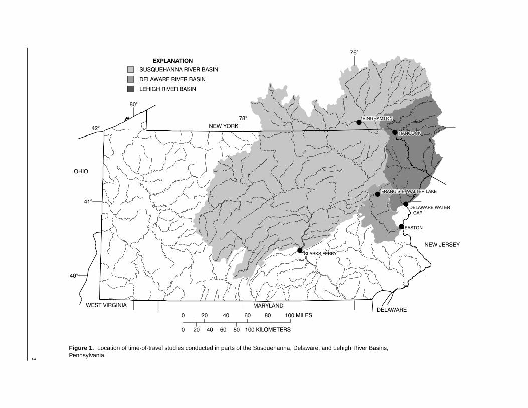
A time-of-travel study was conducted on the Susquehanna River during periods of low flowduring 1965-67 by Kauffman and others (1976) (fig. 1). Time-of-travel studies also wereconducted on the upper Delaware River during periods of low and median flow in 1991 (Whiteand Kratzer, 1994) and on the Lehigh River during periods of low and median flow during1970-77 (Kauffman, 1982) (fig. 1). Velocity data from slope-area measurements in stream reachesnear stream-gaging stations have been collected after periods of high water by USGS from about1965-99. Velocity data were provided in flood-insurance studies (Federal EmergencyManagement Agency, 1978-99) conducted for stream reaches near stream-gaging stations inPennsylvania. Jobson (1996, 1997) developed equations to predict traveltime of low andmoderate flows in streams in the United States. None of the above data sources were used in thedevelopment of Jobson’s equations.
Prediction of Stream Velocities with the Jobson Equation
Regression equations were developed by Jobson (1996) to predict traveltime and dispersionof a soluble, conservative constituent in streams and rivers nationwide for low to moderate flow.Data from approximately 90 different rivers and streams were used to develop the equations anda total of 986 data points were used. The equations were based on drainage area, the reach slope,the mean annual discharge, and the discharge at the time of the measurement (Jobson, 1996).The velocities used in the development of the equation for velocity of peak concentration rangedfrom 0.01 m/s (0.03 ft/s) to 1.51 m/s (4.95 ft/s) with more than 90 percent of the velocities lessthan 2.0 ft/s (Jobson, 1996).
The equation recommended by Jobson (1996) for predicting traveltime of the peakconcentration of a conservative constituent, modified for English units, is
whereV(p) is mean stream velocity of peak concentration of a slug of a dissolved
constituent, in feet per second.The factor 0.0656 has units of feet per second; and
Da′ = (Da1.25 × g0.5)/Qa, (2)
whereDa is drainage area, in square feet;
g is acceleration of gravity, in feet per second squared; andQa is mean annual streamflow, in cubic feet per second; and
Qa′ = Q/Qa, (3)
whereQ is streamflow at the time of interest, in cubic feet per second; and
Qa is mean annual streamflow, in cubic feet per second.
2
3
Basins,
Figure 1. Location of time-of-travel studies conducted in parts of the Susquehanna, Delaware, and Lehigh RiverPennsylvania.
As an example, the velocity of the maximum concentration of a dye cloud for a time-of-travel study on the Susquehanna River between Shickshinny and Danville was 1.16 ft/s. Thedrainage area of the river at Shickshinny is about 10,600 mi2 (2.955 × 1011 ft2), and the meanannual streamflow for the period of record at Shickshinny, on the basis of data from the stream-gaging station at Danville, is about 14,360 ft3/s. At the time of the study, the streamflow was3,610 ft3/s.
Note the velocity calculated by use of Jobson’s equation, 1.19 ft/s, is within 3 percent of themeasured velocity of 1.16 ft/s.
COMPARISON OF STREAM VELOCITIES COMPUTED USING THE JOBSON EQUATIONWITH VELOCITIES DETERMINED FROM OTHER SOURCES
To evaluate the applicability of Jobson’s equation for predicting velocities for a range of lowto high flows in streams in Pennsylvania, velocities computed by use of the Jobson equation werecompared to velocities determined during time-of-travel studies, and to velocities determinedfrom indirect methods used in slope-area measurements, and to velocities determined in flood-insurance studies.
Time-of-Travel Studies
Time-of-travel studies are conducted by adding a traceable constituent to a river anddetermining the time required for the tracer to arrive at and pass selected downstream points ina study reach. This information is crucial in the event of a contaminant spill. The velocitiesdetermined from time-of-travel studies are dependent on the discharge and the hydrauliccharacteristics of a river. Collecting time-of-travel data at two (or more) different discharges candefine a relation through the study reach that integrates the combination of discharge andhydraulics. For example, velocity usually increases and traveltime decreases as the dischargeincreases. If a selected reach of a river has a deep pool, the velocity may be slower and thetraveltime may be longer than those determined from a reach with uniform depths. Time-of-travel studies in Pennsylvania have been limited to the Susquehanna, Delaware, and LehighRivers. These studies are discussed below and the study areas are shown on figure 1.
Susquehanna River
Time-of-travel studies were conducted on the Susquehanna River at low or moderately lowflow at six times during 1965-67 (Kauffman and others, 1976). Flows during the studies rangedfrom 67- to 98-percent exceedence probability, which is the percentage of time flows are equalledor exceeded based on the gaged period of record. The river between Binghamton, N.Y., andClarks Ferry, Pa. (fig. 1), was divided into 17 reaches. Velocities obtained for the reaches by thetime-of-travel studies are compared to velocities predicted by the Jobson equation forcorresponding flows in figure 2. Velocities from the time-of-travel studies ranged from 0.22 ft/s to1.86 ft/s. Although the Jobson equation tended to overestimate at low velocities, the velocitiespredicted by the Jobson equation generally are in good agreement with those measured during
4
the time-of-travel studies (fig. 2). The mean and standard deviation of the measured velocitieswere 1.05 and 0.40 ft/s, respectively, and the mean and standard deviation of the velocitiespredicted by the Jobson equation were 1.08 and 0.27 ft/s, respectively. The standard error of thedifferences in velocities predicted by the Jobson equation and the time-of-travel studies on theSusquehanna River was 0.24 ft/s.
Delaware River
Time-of-travel studies were conducted on the Delaware River from Hancock, N.Y., toDelaware Water Gap, Pa. (fig. 1), in May and August of 1991 (White and Kratzer, 1994). The Maystudy was conducted when river flows ranged from 25- to 30-percent exceedence probability, andthe August study was conducted when river flows ranged from 85- to 95-percent exceedenceprobability. The flows from the May study were higher than flows measured during theSusquehanna River studies. The river was divided into 15 reaches. Velocities determined duringthe time-of-travel studies for 14 of the reaches are compared to velocities predicted by the Jobsonequation (fig. 3). The Jobson equation was not used to predict velocities for the reach nearNarrowsburg known as the Narrowsburg pool and eddy because depths in the Narrowsburg poolexceed 110 ft and traveltime in the pool, which is about 0.5 mi long, is not representative of therest of the river. Velocities measured during the May study ranged from 1.76 to about 2.71 ft/s,and velocities measured during the August study ranged from 0.64 to about 1.18 ft/s. The meanand standard deviation of the measured velocities were 1.59 and 0.71 ft/s, respectively, and themean and standard deviation of the velocities predicted by the Jobson equation were 1.47 and0.62 ft/s, respectively. The standard error of the differences in velocities predicted by the Jobsonequation from the time-of-travel studies on the Delaware River was 0.31 ft/s.
Figure 2. Comparison of velocities from time-of travel studies (Kauffman and others, 1976) and thosepredicted by the Jobson equation (Jobson, 1996) for reaches of the Susquehanna River fromBinghamton, N.Y., to Clarks Ferry, Pa.
5
Lehigh River
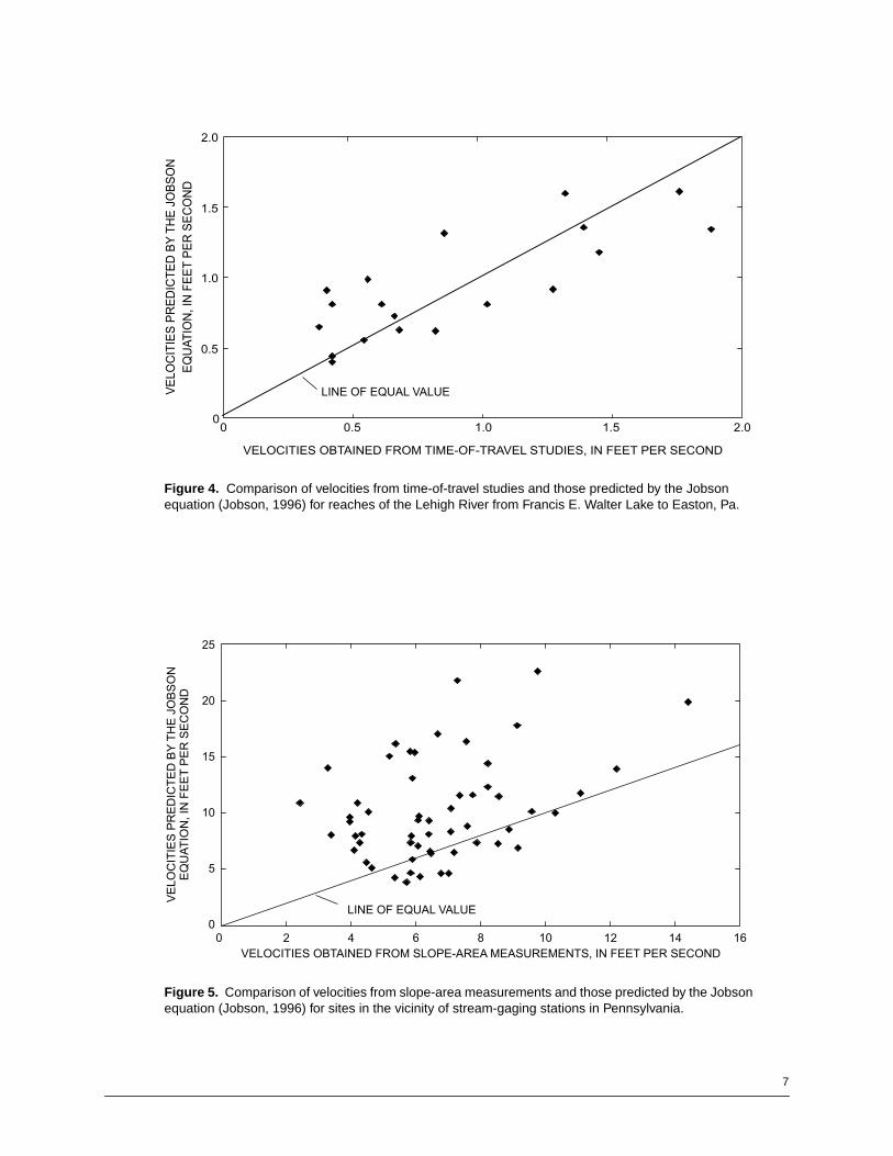
Time-of-travel studies were conducted on the Lehigh River from the outlet of Francis E.Walter Lake to Easton (fig. 1) four times during 1970 to 1977 (Kauffman, 1982). The streamflowson the Lehigh River were at 42-percent exceedence probability during the 1970 study, 80 percentduring the 1973 study, 67 percent during the 1974 study, and 92 percent during the 1977 study.Velocities determined from the time-of-travel studies on the Lehigh River are compared infigure 4 to velocities predicted by Jobson’s equation. Velocities from the time-of-travel studiesranged from 0.37 ft/s to 1.88 ft/s. The mean and standard deviation of the measured velocitieswere 0.89 and 0.48 ft/s, respectively, and the mean and standard deviation of velocities predictedby the Jobson’s equation are 0.93 and 0.37 ft/s, respectively. The standard error of the differencein velocities predicted by Jobson’s equation to the measured velocities on the Lehigh River was0.30 ft/s.
Slope-Area Measurements
Slope-area measurements made in the vicinity of stream-gaging stations in the Delawareand Susquehanna River Basins were reviewed and the mean velocity, streamflow, drainage area,and number of cross-sections were tabulated. A comparison between velocities computed fromthe slope-area measurements and velocities computed by use of the Jobson equation for the57 slope-area measurements is shown in figure 5. Many of the slope-area measurements hadmean velocities that exceeded the maximum velocity used in the development of the Jobsonequation but were included in the comparison to evaluate Jobson’s equation at higher flows.Velocities from the slope-area measurements ranged from 2.43 to 14.4 ft/s. Velocities predicted bythe Jobson equation averaged about 40 percent higher than those determined by the slope-areameasurements. The mean and standard deviation of the velocities determined by the slope-areameasurements were 6.67 and 2.26 ft/s, respectively. The mean and standard deviation of thevelocities computed by use of the Jobson equation were 9.70 and 4.05 ft/s, respectively. Thestandard error of the velocities computed by use of the Jobson equation relative to meanvelocities from the slope-area measurements was 4.10 ft/s.
Figure 3. Comparison of velocities from time-of-travel studies and those predicted by the Jobson equation(Jobson, 1996) for reaches of the Delaware River from Hancock, N.Y., to Delaware Water Gap, Pa.
6
Figure 4. Comparison of velocities from time-of-travel studies and those predicted by the Jobsonequation (Jobson, 1996) for reaches of the Lehigh River from Francis E. Walter Lake to Easton, Pa.
Figure 5. Comparison of velocities from slope-area measurements and those predicted by the Jobsonequation (Jobson, 1996) for sites in the vicinity of stream-gaging stations in Pennsylvania.
7
Current-meter measurements, contracted-opening measurements, and flow-over-dammeasurements were not used in the evaluation. Velocities obtained from current-metermeasurements of streamflow were not used because many of these measurements have beenmade by wading at or near riffles where the flow is confined and velocities are higher than themean velocity in a reach of the stream or river. Current-meter measurements of streamflow canalso be made by suspending a meter from a bridge. Because many bridges were built at a naturalnarrow point or the bridge itself provides some constriction to flow, velocities from thesemeasurements also are higher than the mean velocity of a nearby reach of the stream or riverand therefore were not used. Because velocities obtained from contracted-opening and flow-over-dam measurements do not represent mean velocities in long stream reaches, they were not used.
Flood-Insurance Studies
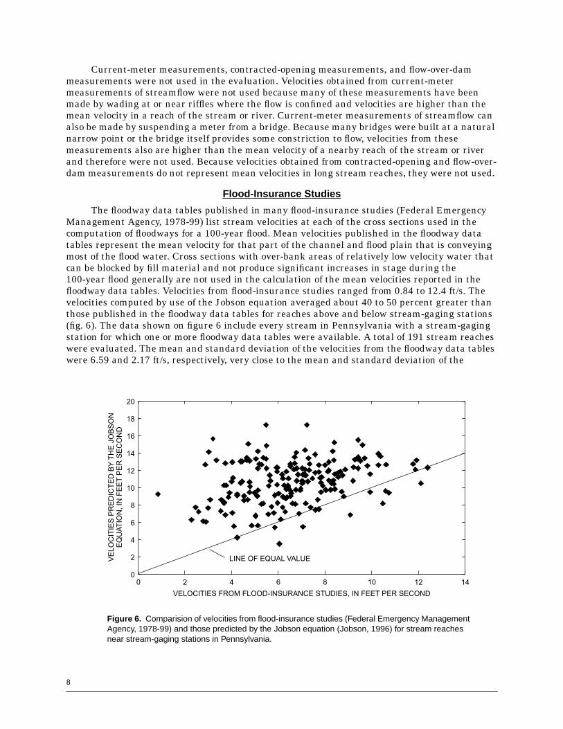
The floodway data tables published in many flood-insurance studies (Federal EmergencyManagement Agency, 1978-99) list stream velocities at each of the cross sections used in thecomputation of floodways for a 100-year flood. Mean velocities published in the floodway datatables represent the mean velocity for that part of the channel and flood plain that is conveyingmost of the flood water. Cross sections with over-bank areas of relatively low velocity water thatcan be blocked by fill material and not produce significant increases in stage during the100-year flood generally are not used in the calculation of the mean velocities reported in thefloodway data tables. Velocities from flood-insurance studies ranged from 0.84 to 12.4 ft/s. Thevelocities computed by use of the Jobson equation averaged about 40 to 50 percent greater thanthose published in the floodway data tables for reaches above and below stream-gaging stations(fig. 6). The data shown on figure 6 include every stream in Pennsylvania with a stream-gagingstation for which one or more floodway data tables were available. A total of 191 stream reacheswere evaluated. The mean and standard deviation of the velocities from the floodway data tableswere 6.59 and 2.17 ft/s, respectively, very close to the mean and standard deviation of the
Figure 6. Comparision of velocities from flood-insurance studies (Federal Emergency ManagementAgency, 1978-99) and those predicted by the Jobson equation (Jobson, 1996) for stream reachesnear stream-gaging stations in Pennsylvania.
8
velocities from the data set from slope-area measurements. The mean and standard deviation ofthe velocities computed by use of the Jobson equation were 10.6 and 2.50 ft/s, respectively. Thestandard error of the velocities computed by use of the Jobson equation relative to velocities fromthe floodway data tables was 2.77 ft/s.
PREDICTION OF VELOCITIES FOR A RANGE OFSTREAMFLOW CONDITIONS IN PENNSYLVANIA
The evaluation of Jobson’s equations for use in high-flow conditions showed that theequations tended to overestimate velocities during high flows. This meant the equation could notbe used to accurately predict velocities above the maximum velocity of 4.95 ft/s that was used inthe development of the equation. Therefore, a new equation was developed to predict velocities inPennsylvania streams using data from the time-of-travel studies on the Susquehanna, Delaware,and Lehigh Rivers, from the slope-area measurements, and from the floodway data tables in theflood-insurance studies.
Development of a New Equation for Predicting Stream Velocities
The two most important variables for predicting stream velocities in Pennsylvania arestreamflow and drainage area. Many other variables could be included in an equation to predictvelocity including stream slope, channel roughness, cross-sectional area at bank full stage,channel storage at low flow, and over-bank storage at high flow. For Pennsylvania streams,recurrence-interval discharges are related closely to drainage area raised to varying coefficients(Flippo, 1982).
Stuckey and Reed (2000) developed regression equations for predicting flows withrecurrence intervals of 10, 25, 50, 100, and 500 years. These equations include the term drainagearea raised to a coefficient that ranges from 0.678 to 0.777 depending on the recurrence intervaland the region of the State. The median of these coefficients is 0.73, excluding that for the500-year flood due to the extremity of the flood event. The 0.73 coefficient was used to develop arelation for predicting stream velocities for specific streamflow, based on discharge divided bydrainage area as shown below.
Q/DA0.73
A measure of the recurrence interval of each of the flows in the three data sets wasdetermined. A scatter plot is shown in figure 7 of the streamflow of interest divided by drainagearea raised to the 0.73 coefficient plotted against the measured velocities from the time-of-travelstudies in the Susquehanna, Delaware, and Lehigh Rivers, the velocities computed from slope-area measurements, and the velocities reported in floodway data tables in the flood-insurancestudies. The regression equation describing the relation shown in figure 7 is given below.
V = 0.6067 e[0.8834 (log(Q/DA0.73))], (4)
whereV is velocity, in feet per second;e is log to base e;
log is log to base 10;Q is streamflow, in cubic feet per second; and
DA is drainage area, in square miles.
This new regression equation has standard errors of estimate of 0.18 ft/s, 0.37 ft/s, and 0.31 ft/s forreaches with time-of-travel studies on the Susquehanna, Delaware, and Lehigh Rivers, respectively.The standard error of estimate is 1.71 ft/s for the slope-area measurements, and 1.22 ft/s for datafrom the floodway data tables. The equation has a coefficient of determination (R2) equal to 0.83.
9
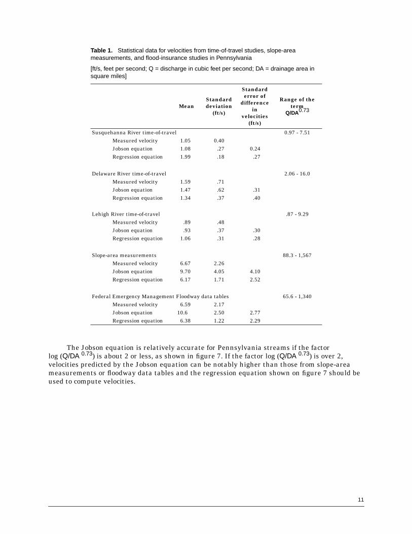
Standard errors for the regression equation shown in figure 7 and statistical data for velocities fromtime-of-travel studies, slope-area measurements, and flood-insurance studies are summarized intable 1. A comparison between velocities predicted by the regression equation and the measuredvelocities from the time-of-travel studies and the computed velocities from the slope-areameasurements and flood-insurance studies is shown in figure 8.
Figure 7. Relation between log (Q/DA0.73) and stream velocities from time-of-travel studies, slope-area measurements, and flood-insurance studies in Pennsylvania.
Figure 8. Comparison of stream velocities predicted by the new regression equation and those fromtime-of-travel studies, slope-area measurements, and flood-insurance studies in Pennsylvania.
10
The Jobson equation is relatively accurate for Pennsylvania streams if the factorlog (Q/DA 0.73) is about 2 or less, as shown in figure 7. If the factor log (Q/DA 0.73) is over 2,velocities predicted by the Jobson equation can be notably higher than those from slope-areameasurements or floodway data tables and the regression equation shown on figure 7 should beused to compute velocities.
Table 1. Statistical data for velocities from time-of-travel studies, slope-areameasurements, and flood-insurance studies in Pennsylvania
[ft/s, feet per second; Q = discharge in cubic feet per second; DA = drainage area insquare miles]
Federal Emergency Management Floodway data tables 65.6 - 1,340Measured velocity 6.59 2.17Jobson equation 10.6 2.50 2.77Regression equation 6.38 1.22 2.29
11
Considerations and Limitations of Available Velocity Datafor Streams in Pennsylvania
Time-of-travel data are not available for periods of high flow, and the relation betweenvelocities from slope-area measurements and actual velocities in long stream reaches duringperiods of high flow is not known. The relation between traveltime obtained from data publishedin the floodway data tables of flood-insurance studies and actual stream velocities also is notknown. Floodway velocities are not measured data; rather, they are determined based on amaximum 1-ft rise in the 100-year water-surface elevation while encroaching the 100-year floodplain boundary. These velocities may not always duplicate real streamflow conditions. Velocitiescomputed from the slope-area measurements and those published in the floodway data tables ofthe flood-insurance studies have similar means (6.67 and 6.59 ft/s, respectively) and a similarstandard deviation (2.26 and 2.17 ft/s, respectively). Although the two sets of velocities aresimilar, it should be noted that both numbers are computed from the same open-channelequations. Further analysis of equations to predict stream velocities at high flows would beneeded if time-of-travel studies are conducted at high flows.
The Jobson equation works reasonably well for Pennsylvania streams if the factorlog (Q/DA0.73) is 2.0 or less; however, it tends to overpredict velocities if the factor log (Q/DA0.73)is greater than 2.0. The new regression equation can be used throughout the range of flowconditions up to the 100-year flood event. The velocities used to develop the equation rangedfrom 0.22 to 14.4 ft/s. Streams used in the analysis and development of the equation haddrainage areas from 2.4 to 26,000 mi2 and discharges from 58 to 740,000 ft3/s.
12
SUMMARY
The USGS, in cooperation with PaDEP, delineated the boundaries for the 5- and 25-hourtraveltimes of public surface-water-supply intakes on Pennsylvania streams. To determine thesetraveltimes, a method of calculating mean stream velocity over a range of streamflow conditionswas required. Equations to predict traveltime in streams in the United States were presented byJobson (1996, 1997). Most of the data used to develop the equations were collected during periodsof low and moderate flow and none of the data were from Pennsylvania streams. Three data setswere used to evaluate the Jobson equation for Pennsylvania streams over a range of low to highflows: time-of-travel studies on the Susquehanna, Delaware, and Lehigh Rivers, slope-areameasurements of flood flows, and velocities of the 100-year floodway as reported in flood-insurance studies.
A comparison of velocities computed from the traveltime regression equation by Jobson tovelocities measured during the time-of-travel studies showed good agreement for low andmoderately low flow. Comparison of velocities computed with the Jobson regression equation tovelocities from slope-area measurements of high flows and to velocities of the 100-year floodwayfrom various flood-insurance studies (Flood Emergency Management Agency, 1978-99) indicatedthat velocities were over-estimated by the regression equation. Although the low and moderate-flow comparisons showed good agreement, an equation was needed for computing velocitiesduring the range of low to high flows commonly experienced in Pennsylvania streams.
A new regression equation was developed to predict velocities from 0.22 to 14.4 ft/s forstreams in Pennsylvania. This new regression equation was developed using data from threesources: 1) time-of-travel studies conducted at low and moderate flow, 2) slope-areameasurements of flood flows, and 3) velocities of the 100-year floodway as reported in flood-insurance studies. The regression equation had standard errors from 0.18 to 0.37 for the time-of-travel studies, 1.71 for the slope-area measurements, and 1.22 for the flood-insurance studies.
REFERENCES CITED
Federal Emergency Management Agency, 1978-99, Flood insurance studies (About 50 townships andboroughs in Pennsylvania): Washington, D.C. [variously paged] (http://www.fema.gov/maps/).
Flippo, H.N., Jr., 1982, Evaluation of the streamflow-data program in Pennsylvania:U.S. Geological Survey Water-Resources Investigations Report 82-21, 56 p.
Jobson, H.E., 1996, Prediction of traveltime and longitudinal dispersion in rivers and streams:U.S. Geological Survey Water-Resources Investigations Report 96-4013, 69 p.
_____1997, Predicting travel time and dispersion in rivers and streams: Journal of HydraulicEngineering, November 1997, p. 971-978.
Kauffman, C.D., Jr., 1982, Time-of-travel and dispersion studies, Lehigh River, Francis E. WalterLake to Easton, Pennsylvania: U.S. Geological Survey Open-File Report 82-861, 32 p.
Kauffman, C.D., Jr., Armbruster, J.T., and Voytik, Andrew, 1976, Time-of-travel studies SusquehannaRiver, Binghamton, New York to Clarks Ferry, Pennsylvania: U.S. Geological Survey Open-FileReport 76-247, 24 p.
Stuckey, M.H., and Reed, L.A., 2000, Techniques for estimating magnitude and frequency of peakflows for Pennsylvania streams: U.S. Geological Survey Water-Resources InvestigationsReport 00-4189, 43 p.
White, K.E., and Kratzer, T.W., 1994, Determination of traveltime in the Delaware River, Hancock,New York, to the Delaware Water Gap by use of a conservative dye tracer:U.S. Geological Survey Water-Resources Investigations Report 93-4203, 54 p.