Understanding dominant controls on streamflow spatialvariability to set up a semi-distributed hydrologicalmodel: the case study of the Thur catchmentMarco Dal Molin1,2,3, Mario Schirmer2,3, Massimiliano Zappa4, and Fabrizio Fenicia1
1Department Systems Analysis, Integrated Assessment and Modelling, Eawag,Swiss Federal Institute of Aquatic Science and Technology, 8600 Dübendorf, Switzerland2The Centre of Hydrogeology and Geothermics (CHYN), University of Neuchâtel, 2000 Neuchâtel, Switzerland3Department of Water Resources and Drinking Water, Eawag, Swiss FederalInstitute of Aquatic Science and Technology, 8600 Dübendorf, Switzerland4Hydrological Forecast, Swiss Federal Research Institute WSL, 8903 Birmensdorf, Switzerland
Received: 5 March 2019 – Discussion started: 8 March 2019Revised: 7 February 2020 – Accepted: 10 February 2020 – Published: 20 March 2020
Abstract. This study documents the development of a semi-distributed hydrological model aimed at reflecting the dom-inant controls on observed streamflow spatial variability.The process is presented through the case study of theThur catchment (Switzerland, 1702 km2), an alpine and pre-alpine catchment where streamflow (measured at 10 sub-catchments) has different spatial characteristics in terms ofamounts, seasonal patterns, and dominance of baseflow. Inorder to appraise the dominant controls on streamflow spa-tial variability and build a model that reflects them, we fol-low a two-stage approach. In a first stage, we identify themain climatic or landscape properties that control the spa-tial variability of streamflow signatures. This stage is basedon correlation analysis, complemented by expert judgementto identify the most plausible cause–effect relationships. Ina second stage, the results of the previous analysis are usedto develop a set of model experiments aimed at determin-ing an appropriate model representation of the Thur catch-ment. These experiments confirm that only a hydrologicalmodel that accounts for the heterogeneity of precipitation,snow-related processes, and landscape features such as ge-ology produces hydrographs that have signatures similar tothe observed ones. This model provides consistent resultsin space–time validation, which is promising for predictionsin ungauged basins. The presented methodology for modelbuilding can be transferred to other case studies, since the
data used in this work (meteorological variables, streamflow,morphology, and geology maps) are available in numerousregions around the globe.
1 Introduction
Semi-distributed rainfall–runoff models are widely appliedin operation for applications such as flood forecasting (e.g.Ajami et al., 2004) or developing sustainable irrigation prac-tices (e.g. McInerney et al., 2018). The main purpose of thesemodels is to simulate streamflow at a limited number of fixedpoints along river channels (e.g. Boyle et al., 2001), and forthis reason they are characterized by a coarser spatial reso-lution than fully distributed models, which allow a very de-tailed representation of the spatial variability of catchmentprocesses. Compared to fully distributed models, they arecharacterized by lower data and computational requirements,which represents a valuable practical advantage in their op-erational use.
Similarly to the case of lumped models, the parametersof semi-distributed models are estimated via calibration.Therefore, it is important that the structure of these modelsis commensurate with the available data, including length,timescale, and spatial distribution (Wooldridge et al., 2001).However, semi-distributed models, even when used for sim-
Published by Copernicus Publications on behalf of the European Geosciences Union.
1320 M. Dal Molin et al.: Understanding dominant controls on streamflow spatial variability
ilar applications such as streamflow predictions, differ sig-nificantly in terms of their process representation as well asthe number of calibration parameters. For example, Gao etal. (2014) assume topography to be a dominant control onhydrological processes, whereas the SWAT model (Arnold etal., 1998) emphasizes the role of soil properties. These dif-ferences raise the question of how to select an appropriatemodel structure for the data at hand, which requires under-standing of the association between model parameters andthe climatological and geomorphological characteristics ofthe catchment.
Understanding the relationship between climate, land-scape, and catchment response is a common objective ofmany research areas in hydrology, including comparative hy-drology (e.g. Falkenmark and Chapman, 1989), model re-gionalization (e.g. Parajka et al., 2005), catchment classifica-tion (e.g. Wagener et al., 2007), and prediction in ungaugedbasins (e.g. Hrachowitz et al., 2013). In the case of stream-flow, the attempt to explain its spatial variability is typicallyaccomplished either using statistical approaches, which aredesigned to regionalize selected characteristics of the hydro-graph (streamflow signatures), or through hydrological mod-els that account for relevant spatial information. In particular,statistical approaches such as regression analysis (e.g. Bergerand Entekhabi, 2001; Bloomfield et al., 2009) and correla-tion analysis (e.g. Trancoso et al., 2017), or machine learn-ing techniques like clustering (e.g. Sawicz et al., 2011; Toth,2013; Kuentz et al., 2017), are used to group together catch-ments that present similar characteristics and to extrapolatethe signatures where unknown. Such approaches have beenuseful for quantifying the hydrological variability and iden-tifying its principal drivers. However, they are often not de-signed to discover causality links and can be affected by mul-ticollinearity, which arises when multiple factors are corre-lated internally and with the target variable (Kroll and Song,2013).
By incorporating spatial information about meteorologi-cal forcings and landscape characteristics, semi-distributedhydrological models have the ability to mimic the mecha-nisms that influence hydrograph spatial variability. However,identifying the relevant mechanisms is challenging. One pos-sibility is to be as inclusive as possible in accounting forall the catchment properties that are, in principle, importantin controlling catchment response. However, this approachleads to models that tend to be data demanding and containmany parameters. For example, Gurtz et al. (1999) consid-ered several landscape characteristics (elevation, land use,etc.) in their application of a semi-distributed model to theThur catchment (Switzerland), which resulted in a modelwith hundreds of hydrological response units (HRUs) thatwere defined a priori based on the complexity of the catch-ment. The other option is to try to identify the most relevantprocesses and neglect others in order to control model com-plexity. For example, Fenicia et al. (2016) compared variousmodel hypotheses to determine an appropriate discretization
of the catchment in HRUs and appropriate structures for dif-ferent HRUs. Antonetti et al. (2016) used a map of domi-nant runoff processes following Scherrer and Naef (2003) fordefining HRUs. However, these approaches require a goodexperimental understanding of the area, which is not alwaysavailable.
Convincing model calibration–validation strategies are es-sential to provide confidence that the model ability to fit ob-servations is a reflection of model realism and not a conse-quence of calibrating an overparameterized model (e.g. An-dréassian et al., 2009). A common approach for the cali-bration of semi-distributed models is the so-called “sequen-tial” approach, where subcatchments are calibrated sequen-tially from upstream to downstream (e.g. Verbunt et al., 2006;Feyen et al., 2008; Lerat et al., 2012; De Lavenne et al.,2016). Although this approach may provide good fits andtherefore has its practical utility where data are available,it does not provide understanding of the causes of stream-flow spatial variability and results in models that are not spa-tially transferable. Moreover, such models are prone to con-tain many parameters, as each subcatchment would be repre-sented by its own set of parameters. Alternative calibration–validation approaches that enable model validation not onlyin time but also in space are conceptually preferable, particu-larly when the modelling is used for process understanding orprediction in ungauged locations (e.g. Wagener et al., 2004;Fenicia et al., 2016).
The objective of this study is to develop a semi-distributedhydrological model with the appropriate level of functionalcomplexity to reproduce streamflow spatial variability in theThur catchment. For this purpose, we use a two-stage ap-proach, the first one dedicated to an in-depth analysis of theavailable data and the second one focused on hydrologicalmodelling.
Our specific objectives are to (1) explore the spatial vari-ability present in the Swiss Thur catchment regarding land-scape characteristics, meteorological forcing, and streamflowsignatures; (2) identify the main climate and landscape con-trols that explain the variability of the hydrological response;(3) based on this analysis, build a set of model experimentsaimed to test the relative importance of dominant processesand their effect on the hydrograph; and (4) appraise modelassumptions against competing alternatives using a stringentvalidation strategy.
The paper is organized as follows: Sect. 2 presents thestudy area and gives information about data availability;Sect. 3 illustrates the methodology; Sect. 4 shows the re-sults; Sect. 5 analyses the results and puts them in perspec-tive, showing what other similar studies have found; Sect. 6,finally, summarizes the main conclusions.
M. Dal Molin et al.: Understanding dominant controls on streamflow spatial variability 1321
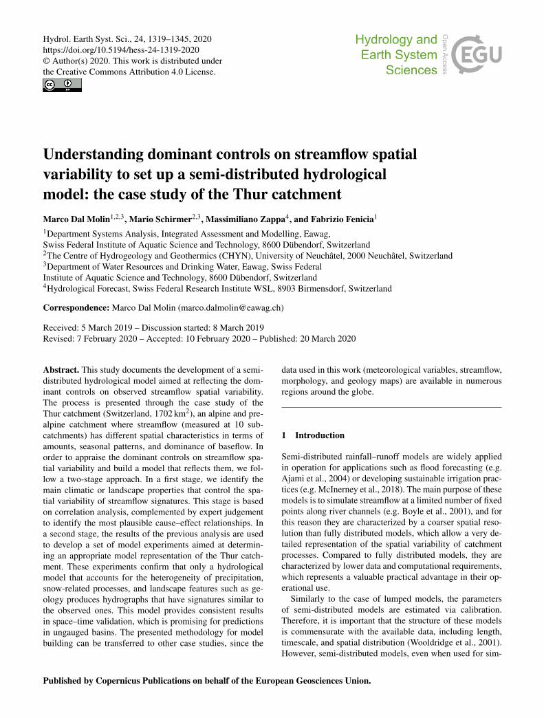
Figure 1. Landscape characteristics of the Thur catchment: (a) subdivision into subcatchments, river network, and gauging stations; (b) ele-vation map; (c) land-use map; (d) simplified geology map; (e) soil depth map; (f) slope map (derived from the elevation map).
2 Study area
This study is carried out in the Thur catchment (Fig. 1), lo-cated in the north-east of Switzerland, south-west of LakeConstance. With a total length of 127 km and a catchmentarea of 1702 km2, the Thur is the longest Swiss river, with-out any natural or artificial reservoir along its course. TheThur River is very dynamic, with streamflow values thatcan change by 2 orders of magnitude within a few hours(Schirmer et al., 2014).
The Thur catchment has been the subject of several stud-ies in the past: Gurtz et al. (1999) performed the first mod-elling study on the entire catchment using a semi-distributedhydrological model; Abbaspour et al. (2007) modelled hy-drology and water quality using the SWAT model; Fundel et
al. (2013) and Jorg-Hess et al. (2015) focused on low flowsand droughts; Jasper et al. (2004) investigated the impact ofclimate change on the natural water budget. Other modellingstudies also include Melsen et al. (2014, 2016), who investi-gated parameter estimation in data-limited scenarios and pa-rameter transferability across spatial and temporal scales, andBrunner et al. (2019), who studied the spatial dependenceof floods. The Thur also includes a small-sized experimentalsubcatchment (Rietholzbach, called Mosnang in this paperafter the name of the gauging station) that was the subjectof many field studies at the interface between process un-derstanding and hydrological modelling (e.g. Menzel, 1996;Gurtz et al., 2003; Seneviratne et al., 2012; von Freyberg etal., 2014, 2015).
∗ Code of the gauging station, as defined by the Federal Officefor the Environment, FOEN.
The topography of the catchment is presented in Fig. 1b;the elevation ranges between 356 m a.s.l. at the outlet and2502 m a.s.l. at Mount Säntis. The majority of the catch-ment lies below 1000 m a.s.l. (75 %) and only 0.6 % isabove 2000 m a.s.l. (Gurtz et al., 1999). Based on topogra-phy (Fig. 1b), the catchment can be visually subdivided intotwo distinct regions: the northern part, with low elevation anddominated by hills and flat land, and the southern part, whichpresents a mountainous landscape.
The land use (Fig. 1c) is dominated by pasture andsparsely vegetated soil (60 %) and forest (25 %); urbanizedand cultivated areas are located mainly in the north and cover7 % and 4 % of the catchment respectively.
Most of the catchment is underlain by conglomerates, marlincrustations, and sandstone (Gurtz et al., 1999). For the pur-pose of this study, the geological formations have been di-vided into three classes (Fig. 1d): “consolidated”, coveringmainly the mountainous part of the catchment, “unconsol-idated”, located in the north, and “alluvial”, located in theproximity of the river network, mainly in the plateau area;the latter formation constitutes the main source of ground-water in the region (Schirmer et al., 2014). The soil depth(Fig. 1e) is shallower in the mountainous part of the catch-ment and deeper in the northern part.
Based on the availability of gauging stations (Table 1), thecatchment was divided into 10 subcatchments (Fig. 1a), witha total drained area that ranges between 3.2 km2 (Mosnang)and 1702 km2 (Andelfingen). Streamflow time series are ob-tained from the Federal Office for the Environment FOEN,and the data are available from 1974 to 2017 but are usedonly from 1981 to 2005 to match the precipitation, temper-ature, and potential evapotranspiration (PET) time series. Inthe considered range, the streamflow data are relatively con-tinuous, with two gaps, one in St. Gallen, from 31 Decem-ber 1981 to 1 January 1983, and the other one in Herisau,from 31 December 1982 to 9 May 1983.
The raw maps (topography, land use, geology, and soil) areobtained from the Federal Office of Topography (swisstopo).The meteorological data are obtained from the Federal Of-fice of Meteorology and Climatology MeteoSwiss. Precipi-tation and temperature are interpolated, as done in Melsen etal. (2016), with the WINMET pre-processing tool (Viviroliet al., 2009) using inverse distance weight (IDW) and de-trended IDW respectively; while the first method considersonly the horizontal variability (related to the distance fromthe meteorological stations), the second adds a vertical com-ponent to the variability related to the elevation (Garen andMarks, 2001). PET data are then obtained, as done in Gurtzet al. (1999), starting from meteorological and land-use data,using the Penman–Monteith equation (Monteith, 1975), im-plemented as part of the PREVAH hydrological model (Vivi-roli et al., 2009). All these values are calculated at pixel(100 m) scale and then averaged over the subcatchments. Allthe time series are used at daily resolution in the subsequentanalyses, aggregating the available hourly data. This choicewas influenced on the one hand by the need to limit the com-putational demand for the model experiments, for which acoarser temporal resolution is preferable, and on the otherhand by the need to represent relevant hydrograph dynamics,for which finer temporal resolution is desirable (e.g. Kavetskiet al., 2011). A daily data resolution, although it may obscuresubdaily process dynamics, appeared to be a good compro-mise, and it is a typical choice in distributed model applica-tions at such spatial scales (e.g. Kirchner et al., 2004).
3 Methods
The methodology follows a two-stage approach. The firststage aims at determining the climatic and landscape con-trols on streamflow signatures. The second stage uses thisunderstanding to configure the structure of a semi-distributedmodel, whose functional suitability is tested through a set ofmodel experiments. Section 3.1 describes the first stage ofthe analysis, that is, the identification of influence factors onthe spatial variability of streamflow signatures. Section 3.2describes the general structure of the semi-distributed modeland the model evaluation approach. The design of the modelexperiments, which is dependent on the outcomes of thefirst stage of analyses, is presented directly in the results(Sect. 4.2.2).
3.1 Identification of influence factors on the spatialvariability of streamflow signatures
The purpose of the analysis presented in this section is to un-derstand the influence of climatic conditions and landscapecharacteristics on streamflow. Climatic conditions are repre-sented by precipitation, potential evaporation, and tempera-ture time series. Landscape characteristics are represented bymaps of topography, land use, geology, and soil.
M. Dal Molin et al.: Understanding dominant controls on streamflow spatial variability 1323
Climatic conditions, landscape characteristics, and stream-flow are represented through a set of statistics (listed in Ta-ble 2). In the following, statistics calculated based on stream-flow data will be called streamflow “signatures”, as is of-ten done in the catchment classification literature (e.g. Siva-palan, 2006). We will refer to climatic and landscape “in-dices” for statistics calculated based on climatic data andlandscape characteristics. A broad list of signatures and in-dices is presented in Sect. 3.1.1; Sect. 3.1.2 presents the ap-proach for reducing such a list to a set of meaningful vari-ables; Sect. 3.1.3 illustrates the approach for determining theindices that mostly control streamflow signatures; Sect. 3.1.4describes how the signature analysis is used to set up themodel experiments.
3.1.1 Catchment indices for representing streamflow,climate, and landscape
Streamflow signatures (ζ ) and climatic indices (ψ) were ob-tained using streamflow, precipitation, PET, and temperaturetime series. The values were calculated using 24 years ofdata, between 1 September 1981 and 31 August 2005; weconsidered 1 September to be the beginning of the hydrologi-cal year. The periods with gaps in the data (refer to Sect. 2 fordetails) were discarded from the analysis of the specific sub-catchment. Landscape indices were obtained using the mapsdescribed in Sect. 2.
Addor et al. (2017) recently compiled a comprehensivelist of streamflow signatures and climatic indices for char-acterizing catchment behaviour (see Table 3 in Addor et al.,2017). Here, we adopted their selection: while being origi-nally introduced for a study about large-sample hydrology,we believe that the indices proposed are also able to captureseveral different aspects of the time series and are thereforealso suitable for this regional study. The streamflow signa-tures considered here are described hereafter, followed by anexplanation of their rationale:
– average daily streamflow ζQ = q, where q is the stream-flow time series and the overbar represents the averageover the observation period;
– runoff ratio ζRR =qp
, where p is the precipitation timeseries;
– streamflow elasticity (ζEL) defined as
ζEL =med((
1q
q
)/
(1p
p
)), (1)
where 1q and 1p represent the streamflow and pre-cipitation difference between two consecutive years andmed is the median function;
– slope of the flow duration curve (ζFDC) definedas the slope between the log-transformed 33rd and66th streamflow percentiles;
– baseflow index ζBFI =q(b)
q, where q(b) represents the
baseflow and was calculated using a low-pass filter asillustrated in Ladson et al. (2013) with the equations
q(f)t =
(0,ϑbq
(f)t−1+
1+ϑb
2(qt − qt−1)
), (2)
q(b)t = qt − q
(f)t , (3)
with q(f)t representing the quickflow. The settings of thefilter were taken according to the findings of Ladsonet al. (2013) and, in particular, three filter passes wereapplied (forward, backward, and forward), the parame-ter ϑb was chosen to be equal to 0.925, and a reflectionof 30 time steps at the beginning and at the end of thetime series was used;
– mean half streamflow date (ζHFD) (Court, 1962), de-fined as the number of days needed in order to have acumulated streamflow that reaches 50 % of the total an-nual streamflow;
– 5th and 95th percentiles of the streamflow (ζQ5 and ζQ95respectively);
– frequency (ζHQF) and mean duration (ζHQD) of high-flow events: they are defined as the days when thestreamflow is bigger than 9 times the median dailystreamflow;
– frequency (ζLQF) and mean duration (ζLQD) of low-flowevents: they are defined as the days when the streamflowis smaller than 0.2 times the mean daily streamflow.
The frequency of days with zero streamflow, present in Ad-dor et al. (2017), was not considered in this study becausethere are no ephemeral subcatchments in the study area.
This group of streamflow signatures is capable of cap-turing various characteristics of the hydrograph: ζQ mea-sures the overall water flows, ζRR represents the propor-tion of precipitation that becomes streamflow, ζEL measuresthe sensitivity of the streamflow to precipitation variations,with a value greater than 1 indicating an elastic subcatch-ment (i.e. sensitive to change in precipitation) (Sawicz etal., 2011), ζFDC measures the variability of the hydrograph,with a steeper flow duration curve indicating a more vari-able streamflow, ζBFI measures the magnitude of the base-flow component of the hydrograph and can be considereda proxy for the relative amount of groundwater flow in thehydrograph, ζHFD measures the streamflow seasonality, ζQ5,ζLQF, and ζLQD measure low-flow dynamics, and ζQ95, ζHQF,and ζHQD measure high-flow dynamics.
Climatology was represented through the following in-dices (see Addor et al., 2017, Table 2):
1324 M. Dal Molin et al.: Understanding dominant controls on streamflow spatial variability
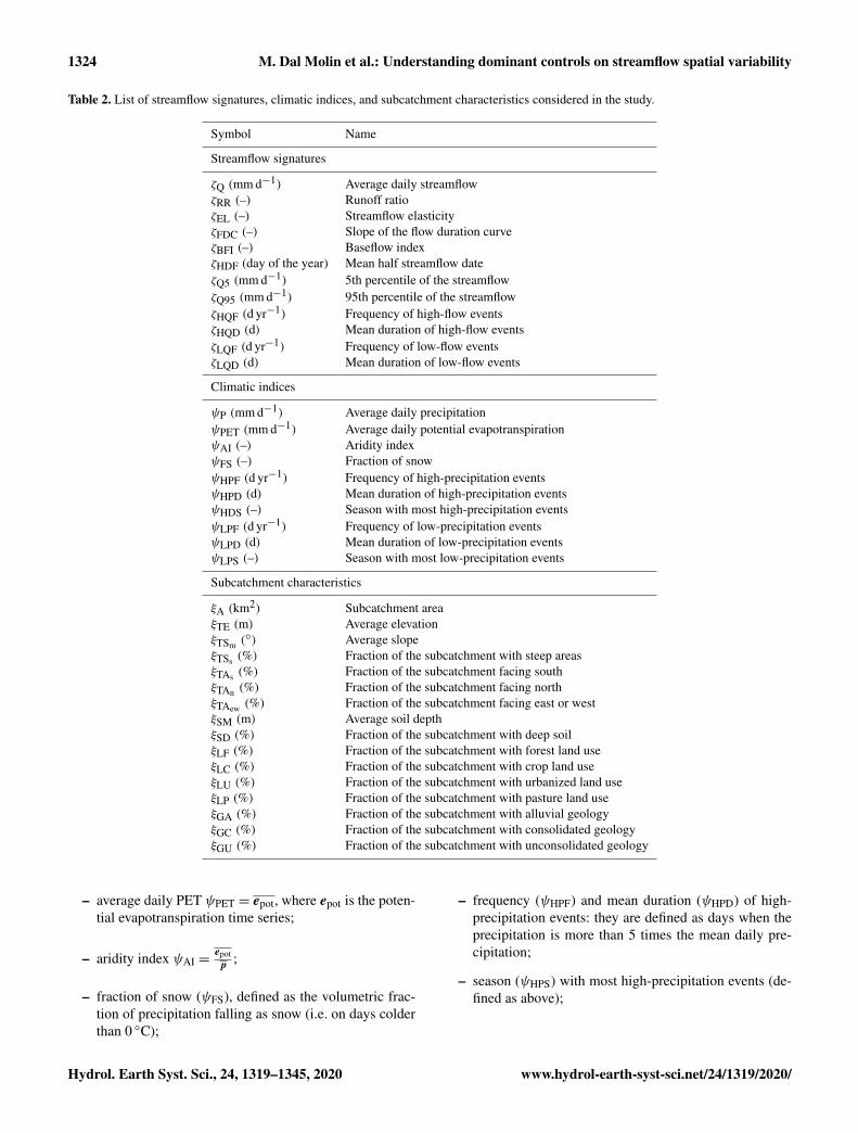
Table 2. List of streamflow signatures, climatic indices, and subcatchment characteristics considered in the study.
Symbol Name
Streamflow signatures
ζQ (mm d−1) Average daily streamflowζRR (–) Runoff ratioζEL (–) Streamflow elasticityζFDC (–) Slope of the flow duration curveζBFI (–) Baseflow indexζHDF (day of the year) Mean half streamflow dateζQ5 (mm d−1) 5th percentile of the streamflowζQ95 (mm d−1) 95th percentile of the streamflowζHQF (d yr−1) Frequency of high-flow eventsζHQD (d) Mean duration of high-flow eventsζLQF (d yr−1) Frequency of low-flow eventsζLQD (d) Mean duration of low-flow events
Climatic indices
ψP (mm d−1) Average daily precipitationψPET (mm d−1) Average daily potential evapotranspirationψAI (–) Aridity indexψFS (–) Fraction of snowψHPF (d yr−1) Frequency of high-precipitation eventsψHPD (d) Mean duration of high-precipitation eventsψHDS (–) Season with most high-precipitation eventsψLPF (d yr−1) Frequency of low-precipitation eventsψLPD (d) Mean duration of low-precipitation eventsψLPS (–) Season with most low-precipitation events
Subcatchment characteristics
ξA (km2) Subcatchment areaξTE (m) Average elevationξTSm (
◦) Average slopeξTSs (%) Fraction of the subcatchment with steep areasξTAs (%) Fraction of the subcatchment facing southξTAn (%) Fraction of the subcatchment facing northξTAew (%) Fraction of the subcatchment facing east or westξSM (m) Average soil depthξSD (%) Fraction of the subcatchment with deep soilξLF (%) Fraction of the subcatchment with forest land useξLC (%) Fraction of the subcatchment with crop land useξLU (%) Fraction of the subcatchment with urbanized land useξLP (%) Fraction of the subcatchment with pasture land useξGA (%) Fraction of the subcatchment with alluvial geologyξGC (%) Fraction of the subcatchment with consolidated geologyξGU (%) Fraction of the subcatchment with unconsolidated geology
– average daily PET ψPET = epot, where epot is the poten-tial evapotranspiration time series;
– aridity index ψAI =epotp
;
– fraction of snow (ψFS), defined as the volumetric frac-tion of precipitation falling as snow (i.e. on days colderthan 0 ◦C);
– frequency (ψHPF) and mean duration (ψHPD) of high-precipitation events: they are defined as days when theprecipitation is more than 5 times the mean daily pre-cipitation;
– season (ψHPS) with most high-precipitation events (de-fined as above);
M. Dal Molin et al.: Understanding dominant controls on streamflow spatial variability 1325
Table 3. Values of the streamflow signatures. The names of the subcatchments are abbreviated using the first three letters and the symbolsare reported in Table 2. The last column contains the coefficient of variation of each signature.
– frequency (ψLPF) and mean duration (ψLPD) of drydays: they are defined as days when the precipitationis lower than 1 mm d−1;
– season (ψLPS) with most dry days (defined as above).
The seasonality of precipitation used in Addor et al. (2017)was not considered in this study as it relied on fitting a sinu-soidal function to the precipitation values, which in our casedid not produce reliable results. Nevertheless, these clima-tological indices are able to comprehensively represent theclimatic conditions of the subcatchment, with ψP represent-ing average water input, ψPET representing average evapo-rative demand, ψAI measuring the dryness of the climate,ψFS measuring the relative importance of snow, ψHPF, ψHPD,and ψHPS measuring the importance of intense precipitationevents, and ψLPF, ψLPD, and ψLPS measuring the importanceof dry days.
The landscape characteristics were divided into four cat-egories: topography, land use, soil, and geology. In orderto quantify the characteristics of each category, a set of in-dices (ξ ) was defined. It is important to notice that all theareas calculated in this analysis were normalized by the re-spective subcatchment area (ξA) in order to get comparablevalues between subcatchments of different sizes.
Topography was represented with the following indices,calculated based on the digital elevation model:
– average elevation (ξTE);
– average slope (ξTSm );
– fraction of the subcatchment with steep areas (ξTSs ),with slope larger than 10◦;
– aspect, i.e. fraction of the subcatchment facingnorth (ξTAn ), south (ξTAs ), or east and west (ξTAew ).
Land use was represented with the following characteristics,obtained by reclassifying the land-use map into four cate-gories (from 22 original classes):
– fraction of the subcatchment with crop land use (ξLC);
– fraction of the subcatchment with pasture landuse (ξLP);
– fraction of the subcatchment with forest land use (ξLF);
– fraction of the subcatchment with urbanized landuse (ξLU).
Soil type was represented with the following indices, derivedby the soil map:
– fraction of the subcatchment with deep soil (soil depthgreater than 2 m) (ξSD);
– average soil depth (ξSM).
Geology was represented by the following indices, obtainedby reclassifying the original map into three categories (from22 original classes):
– fraction of the subcatchment with alluvial geol-ogy (ξGA);
– fraction of the subcatchment with consolidated geol-ogy (ξGC);
– fraction of the subcatchment with unconsolidated geol-ogy (ξGU).
The reclassification of the land use and of the geology mapsconsisted in aggregating specific classes into general classes(e.g. combining different types of forests into a unique forestclass) with the objective of reducing their number, in order tofacilitate subsequent analyses.
1326 M. Dal Molin et al.: Understanding dominant controls on streamflow spatial variability
The consideration of topography, land use, soil, and geol-ogy for defining landscape indices was based on their poten-tial influence on hydrological processes and, in turn, on theshape of the hydrograph. These landscape characteristics canall play an important role in controlling hydrological pro-cesses: land use can, for example, influence the infiltrationof water in the substrate; soil thickness can affect the parti-tioning between water storage and runoff; vegetation is typ-ically assumed to affect evaporation, and geology can affectgroundwater dynamics. Indeed, these characteristics are usedby many semi-distributed hydrological models, for examplefor determining parameter values or for dividing the catch-ment into areas with a homogenous hydrological response(e.g. Gurtz et al., 1999).
3.1.2 Selection of meaningful streamflow signatures,climatic indices, and catchment indices
The sets of statistics presented in Sect. 3.1.1 were designed tobe comprehensive. However, they may also be redundant, forexample by containing metrics that express similar character-istics of the underlying data. In order to facilitate subsequentcorrelation analyses between the various sets of statistics, itis important to reduce each set to a short list of meaningfulvariables. The reduction of each set of streamflow signatures,climatic indices, and landscape indices was achieved throughthe following steps.
– All the statistics that did not show sufficient variabilitybetween the subcatchments were eliminated. We werein fact interested in identifying causes of spatial vari-ability in the streamflow dynamics of the subcatchmentsof the Thur. Therefore, statistics that had a low variabil-ity were not of interest in this analysis. The variabilitywas assessed using the coefficient of variation (definedby the ratio between the standard deviation and the av-erage) and statistics with a value lower than 5 % werediscarded.
– All the catchment indices (e.g. a certain type of landuse) that account for a limited part of any subcatchmentwere discarded. This point was motivated by the ex-pectation that landscape characteristics covering a verysmall fraction of the subcatchment should not have astrong influence on the streamflow signatures consid-ered. Here, landscape indices accounting for less than5 % of any subcatchment area were discarded.
– Within each set of streamflow signatures, climatic in-dices, and catchment indices, we retained only relativelyindependent metrics, if these are believed to representthe same underlying features of the time series. Thisstep was motivated by the need to remove redundantinformation within each set. The selection of indepen-dent metrics was aided by Spearman’s rank score be-tween each pair of metrics, which represents (also non-linear) correlation between variables. Pairs of metrics
with high absolute values of Spearman’s rank score arepotentially redundant. In eliminating potentially redun-dant variables, we adopted the following criteria.
– Among highly correlated metrics, we preferredthose depending on single variables (e.g. only pre-cipitation or only streamflow) to those containingmultiple variables (e.g. combining precipitation andstreamflow or evaporation, such as the runoff ratioor the aridity index), as this may be a problem whenlooking for correlations between metrics.
– With respect to landscape indices, in many cases thehigh correlation is due to the fact that they are com-plementary (the areal fractions sum up to unity). Insuch cases, we kept one index per class (e.g. a sin-gle index for geology).
– A high correlation between metrics does not alwaysmean that the metrics represent the same information.Therefore, the final selection of relevant metrics withineach set was guided by expert judgement.
Based on this process, we compiled a reduced list of sig-natures, climatic indices, and landscape indices, which wasused in subsequent analyses.
3.1.3 Identification of climate and landscape controlson streamflow and consequences for modeldevelopment
This analysis aimed to identify climatic and landscape in-dices that mostly control streamflow signatures. In order toidentify causality links between indices (ψ and ξ ) and signa-tures (ζ ), we proceed as follows:
– we calculated the correlation between indices and sig-natures using Spearman’s rank score and identified pairsof variables with high correlation;
– we scrutinized pairs of variables with high correlationsusing expert judgement to decide whether a causalitylink between variables is justified.
The outcome of this process will be used to inform the semi-distributed model setup. The expert judgement is a criticalstep in the elicitation of causality from correlation (e.g. An-tonetti and Zappa, 2018), and it is clearly subjective, beingdependent on personal experience and subject matter knowl-edge. Although personal and subjective, expert decisions arebased on an attempt to interpret data rather than being a pri-ori defined, which is typically the case in the application ofsemi-distributed hydrological models.
3.1.4 Semi-distributed model setup and modelexperiments
We assumed a generic structure for a semi-distributed hydro-logical model, described in Sect. 3.2.1, where some model
M. Dal Molin et al.: Understanding dominant controls on streamflow spatial variability 1327
structure characteristics are defined a priori and others are tobe defined. In order to motivate the open decisions, we pro-ceeded as follows:
– we used the identified causality links to interpret thedominant processes influencing signature spatial vari-ability;
– we designed model experiments aimed to confirmthe hypothesized climatic and landscape controls onstreamflow spatial variability.
The overall objective of the model experiments is to provethat only models that incorporate the correct dependenciesare able to correctly predict regional streamflow variability.In order to test this assumption, the model experiments willinclude cases where the assumed dependencies are not incor-porated. Omitting an assumed dependency leads to a struc-turally simpler model, which may raise doubt that potentialdifferences in model performance might be due to differencesin model complexity. For this reason, the model experimentswill include cases where alternative dependencies are incor-porated, which do not reduce model complexity. In order tokeep the study and presentation tractable, the model experi-ments will be limited to a few cases, illustrated in Sect. 4.2.1,which we judge relevant for this specific application.
3.2 General structure of the semi-distributedhydrological model and model evaluation approach
This section describes the approach for building and testinga semi-distributed hydrological model designed to representthe observed streamflow and particularly the observed spa-tial variability of streamflow signatures. The general modelstructure is explained in Sect. 3.2.1, the error model and thecalibration procedure are described in Sects. 3.2.2 and 3.2.3,and the metrics utilized to assess the performance are shownin Sect. 3.2.4.
3.2.1 General structure of the hydrological model
We describe here the general model structure; the definitionof specific model experiments, which depends on the resultsof the signature analysis done in the first step, will be de-scribed in Sect. 4.2.2.
The model uses a two-layer decomposition of the catch-ment.
1. Subcatchments are defined by the presence of the gaug-ing stations; this subdivision is due to the necessity ofhaving locations in the model where the streamflow isboth observed and simulated and, therefore, it is possi-ble to calibrate and evaluate the parameters of the hy-drological model.
2. HRUs are defined based on catchment characteristics(e.g. topography, geology, or vegetation); they represent
parts of the catchment that are supposed to have a simi-lar hydrological response to the meteorological forcing.Each HRU is characterized by its own parameterization.Different definitions of HRUs are tested, as described inSect. 4.2.2.
Each HRU has a unique parameterization. However, depend-ing on how the inputs are discretized, the same HRU can havedifferent states in different parts of the catchment. Therefore,the same HRU needs its own model representation when-ever the spatial variability of states needs to be considered.For example, if the inputs are discretized per subcatchment,the same HRU needs a separate model representation in eachsubcatchment where it is present. For more details about ourmodel implementation of HRUs, refer to Fig. 4 of Fenicia etal. (2016).
In order to limit the levels of decisions of the semi-distributed models, some of the aspects of the distributedmodels are fixed a priori, and others are left open. In par-ticular,
– the structure chosen to represent the various HRUs iskept fixed. That is, differences between HRUs will bereflected only through the parameter values.
– The definition of HRUs is left open. In particular, we donot a priori specify which approach is used to discretizethe landscape.
– The spatial discretization of the model inputs is leftopen. Hence, we do not decide in advance which spa-tial discretization of the inputs is most appropriate.
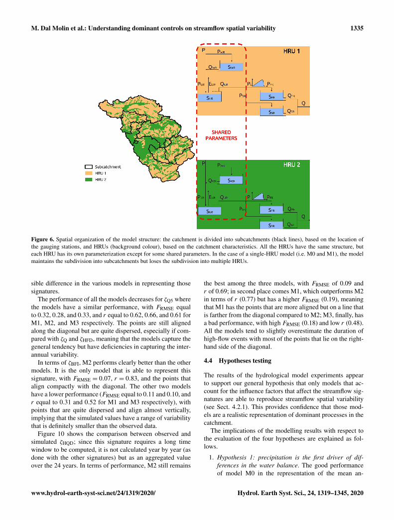
Only the fixed decision about the HRU model structure isdescribed here, whereas the open decisions are describedin the results section (Sect. 4.2.2). The spatial organizationof the model structure is represented in Fig. 6, with theequations listed in Appendix A. The structure includes asnow reservoir (WR), with inputs distributed per subcatch-ments. Snowmelt and rainfall are input to an unsaturatedreservoir (UR), which determines the portion of precipita-tion that produces runoff. This flux is split through a fastreservoir (FR), designed to represent the peaks of the hy-drograph, proceeded by a lag function to offset the hydro-graph, and a slow reservoir (SR), designed to represent base-flow. This structure was chosen to be parsimonious whilegeneral enough to reproduce typical hydrograph behaviour;it was tested in previous applications (e.g. van Esse et al.,2013; Fenicia et al., 2014, 2016), demonstrating its suitabil-ity for reproducing a wide range of catchment responses. Italso resembles popular conceptual hydrological models suchas HBV (Lindstrom et al., 1997) and HyMod (Wagener etal., 2001), which have been shown to have wide applicabil-ity. The model was built using the SUPERFLEX modellingframework (Fenicia et al., 2011).
1328 M. Dal Molin et al.: Understanding dominant controls on streamflow spatial variability
3.2.2 Error model
As commonly done in hydrological modelling (e.g. McIner-ney et al., 2017), we here account for uncertainties by con-sidering a probabilistic model of the observations Q(θ ,x),where θ is the vector of parameters and x the model input,which is composed of a deterministic hydrological modelh(θh,x) (illustrated in Sect. 3.2.1) and a random residualerror term E(θE) that accounts for all data and model un-certainties (θh and θE represent the hydrological and errorparameters):
z[Q(θ ,x);λ] = z [h(θh,x) ;λ]+E(θE) , (4)
where z[y;λ] represents the Box–Cox transformation (Boxand Cox, 1964) with parameter λ, which is used to accountfor heteroscedasticity (stabilize the variance). For λ 6= 0,
z[yt ;λ
]=yλt − 1λ
. (5)
The residual error term is assumed to follow a Gaussian dis-tribution with zero mean and variance σ 2:
Et ∼N(
0;σ 2). (6)
The error model has, therefore, two parameters (λ and σ 2);the first one was fixed to 0.5 (McInerney et al., 2017) and thesecond one was inferred.
This choice of error model (Gaussian noise applied to theBox–Cox transformation of the streamflow) allows for an ex-plicit definition of the likelihood function (McInerney et al.,2017)
p(qobs|θh,θE,x
)=
T∏t=1z′(qobs,t |θE
)fN
(Et |0;σ 2
), (7)
where T represents the length of the time series, fN is theGaussian probability density function (PDF) and z′(qobs|θE)
is the derivative of z(qobs,θE) with respect to q evaluated atthe observed data qobs. Specifying Eq. (5) for the case wherez(qobs;θE) is defined by Eq. (5), the expression of the likeli-hood function becomes
p(qobs|θh,θE,x
)=
T∏t=1q(λ−1)obs,t fN
(Et |0;σ 2
). (8)
Equation (8) represents the likelihood function that is thenused, together with a uniform prior distribution, to calibratethe parameters of the model as described in Sect. 3.2.3.
3.2.3 Calibration
Parameter calibration is performed with the objective of max-imizing their posterior density. According to the Bayes equa-tion, the posterior distribution of model parameters is ex-pressed as the product between the prior distribution and
the likelihood function; since a uniform prior is used forthe parameters, this is equivalent to maximizing the likeli-hood function in the defined parameter space; the optimiza-tion procedure is performed with a multi-start quasi-Newtonmethod (Kavetski et al., 2007) with 20 independent searches.We empirically established that with models of our complex-ity (about 10 parameters), 20 independent searches providegood confidence that a global optimum will be found.
The evaluation of the model ability to reproduce stream-flow is carried out in space–time validation (see also Feniciaet al., 2016). For this purpose, the time domain is dividedinto two periods of 12 years each (from 1 September 1981 to1 September 1993 and from 1 September 1993 to 1 Septem-ber 2005) and the subcatchments are split into two groups(A and B), according to a spatial alternation (subcatchmentin group A flows into a subcatchment in group B that flowsinto one in group A and so on); the subcatchments belongingto group A are Andelfingen, Herisau, Jonschwil, St. Gallen,and Wängi and the ones in group B are Appenzell, Frauen-feld, Halden, Mogelsberg, and Mosnang. This method im-plies a division of the space–time domain into four quad-rants, such that the model can be calibrated in one quadrantand validated in the other three. For space–time validation,the model is calibrated using each group of subcatchmentand period and validated using the other group of subcatch-ment and period. That is, the model calibrated using group Aand period 1 was validated using group B and period 2, andso on for the other three combinations of subcatchments andgroups. The model output in the four space–time validationperiods is then combined to calculate model performance us-ing various indicators (see Sect. 3.2.4). Results are presentedfor space–time validation, which represents the most chal-lenging test of model performance.
3.2.4 Performance assessment
Model performance is assessed using the following metrics.
1. Time series metrics, which evaluate the ability to repro-duce streamflow time series. The metrics used for thisassessment are the following.
– Normalized log likelihood (FLL), that is, the log-arithm of Eq. (8) normalized by the number oftime steps present in the time series. This met-ric corresponds to the objective function used formodel optimization. It can be observed that, sinceλ is fixed at 0.5 in the Box–Cox transformation,model calibration is equivalent to maximizing theNash–Sutcliffe efficiency (FNS) calculated with thesquare root of the streamflow. FLL is not bounded,but a higher value means a better match betweentwo time series since, in this case, the absolutevalue of the residual is smaller and, thus, their PDFhigher.
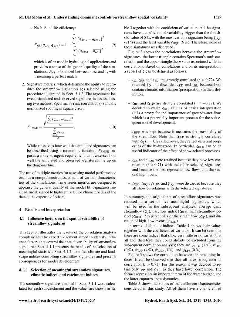
M. Dal Molin et al.: Understanding dominant controls on streamflow spatial variability 1329
– Nash–Sutcliffe efficiency:
FNS(qobs,qsim
)= 1−
T∑t=1
(qsim,t − qobs,t
)2T∑t=1
(qobs,t − qobs
)2 , (9)
which is often used in hydrological applications andprovides a sense of the general quality of the sim-ulations. FNS is bounded between −∞ and 1, with1 meaning a perfect match.
2. Signature metrics, which determine the ability to repro-duce the streamflow signatures (ζ ) selected using theprocedure illustrated in Sect. 3.1.2. The agreement be-tween simulated and observed signatures is assessed us-ing two metrics: Spearman’s rank correlation (r) and thenormalized root mean square error:
FRMSE =
√N∑n=1(ζsim,n−ζobs,n)
2
N
N∑n=1
ζobs,n
N
. (10)
While r assesses how well the simulated signatures canbe described using a monotonic function, FRMSE im-poses a more stringent requirement, as it assesses howwell the simulated and observed signatures line up onthe diagonal line.
The use of multiple metrics for assessing model performanceenables a comprehensive assessment of various characteris-tics of the simulations. Time series metrics are designed toappraise the general quality of the model fit. Signatures, in-stead, are designed to highlight selected characteristics of thedata at the expense of others.
4 Results and interpretation
4.1 Influence factors on the spatial variability ofstreamflow signatures
This section illustrates the results of the correlation analysiscomplemented by expert judgement aimed to identify influ-ence factors that control the spatial variability of streamflowsignatures; Sect. 4.1.1 presents the results of the selection ofmeaningful statistics; Sect. 4.1.2 identifies climate and land-scape indices controlling streamflow signatures and presentsconsequences for model development.
4.1.1 Selection of meaningful streamflow signatures,climatic indices, and catchment indices
The streamflow signatures defined in Sect. 3.1.1 were calcu-lated for each subcatchment and the values are shown in Ta-
ble 3 together with the coefficient of variation. All the signa-tures have a coefficient of variability bigger than the thresh-old value of 5 %, with the most variable signature being ζLQF(71 %) and the least variable ζHQD (6 %). Therefore, none ofthese signatures was discarded.
Figure 2 shows the correlations between the streamflowsignatures: the lower triangle contains Spearman’s rank cor-relation and the upper triangle the p value associated with thecorrelations. Based on correlations and on its interpretation,a subset of ζ can be defined as follows.
– ζQ, ζRR and ζEL are strongly correlated (r > 0.72). Weretained ζQ and discarded ζRR and ζEL because bothcontain climatic information (precipitation) in their def-inition.
– ζBFI and ζFDC are strongly correlated (r =−0.77). Wedecided to retain ζBFI as it is of easier interpretation(it is a proxy for the importance of groundwater flow,which is a potentially important process for the subse-quent model development).
– ζHFD was kept because it measures the seasonality ofthe streamflow. Note that ζHFD is strongly correlatedwith ζQ (r = 0.88). However, they reflect different prop-erties of the hydrograph. In particular, ζHFD can be anuseful indicator of the effect of snow-related processes.
– ζQ5 and ζHQD were retained because they have low cor-relation (r < 0.71) with the other selected signaturesand because the first represents low flows and the sec-ond high flows;
– ζQ95, ζHQF, ζLQD, and ζLQF were discarded because theyall show correlations with the selected signatures.
In summary, the original set of streamflow signatures wasreduced to a set of five meaningful signatures, whichwill be used in the subsequent analyses: average dailystreamflow (ζQ), baseflow index (ζBFI), half streamflow pe-riod (ζHFD), 5th percentiles of the streamflow (ζQ5), and du-ration of high-flow events (ζHQD).
In terms of climatic indices, Table 4 shows their valuestogether with the coefficient of variation. It can be seen thatthere are some indices that show very little or no variation atall and, therefore, they could already be excluded from thesubsequent correlation analysis; they are ψHPD (1 %), ψHPS(0 %), ψLPF (4 %), ψLPD (3 %), and ψLPS (0 %).
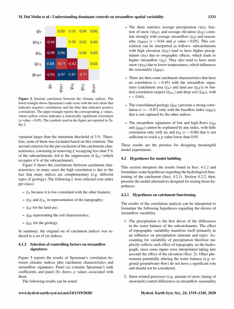
Figure 3 shows the correlation between the remaining in-dices. It can be observed that they all have strong internalcorrelation (r > 0.71). For this reason it was decided to re-tain only ψP and ψFS, as they have lower correlation. Theformer represents an important term of the water budget, andthe latter captures snow dynamics.
Table 5 shows the values of the catchment characteristicsconsidered in this study. All of them have a coefficient of
1330 M. Dal Molin et al.: Understanding dominant controls on streamflow spatial variability
Figure 2. Internal correlation between the streamflow signatures. The lower triangle shows Spearman’s rank score with the red colour thatindicates negative correlations and the blue that indicates positive correlations. The upper triangle reports the corresponding p values, whereyellow colour indicates a statistically significant correlation (p value< 0.05). The symbols used in the figure are reported in Table 2.
Table 4. Values of the climatic indices. The names of the subcatchments are abbreviated using the first three letters and the symbols arereported in Table 2. The last column contains the coefficient of variation of each index.
M. Dal Molin et al.: Understanding dominant controls on streamflow spatial variability 1331
Figure 3. Internal correlation between the climatic indices. Thelower triangle shows Spearman’s rank score with the red colour thatindicates negative correlations and the blue that indicates positivecorrelations. The upper triangle reports the corresponding p values,where yellow colour indicates a statistically significant correlation(p value< 0.05). The symbols used in the figure are reported in Ta-ble 2.
variation larger than the minimum threshold of 5 %. There-fore, none of them was excluded based on this criterion. Thesecond criterion for the pre-exclusion of the catchments char-acteristics, consisting in removing ξ occupying less than 5 %of the subcatchments, led to the suppression of ξLC (whichoccupies 4 % of the subcatchment).
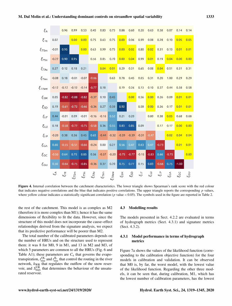
Figure 4 shows the correlations between catchment char-acteristics; in many cases the high correlation is due to thefact that many indices are complementary (e.g. differenttypes of geology). The following ξ were selected (one indexper class):
– ξA because it is low correlated with the other features;
– ξTE and ξTAs in representation of the topography;
– ξLF for the land use;
– ξSD representing the soil characteristics;
– ξGC for the geology.
In summary, the original set of catchment indices was re-duced to a set of six indices.
4.1.2 Selection of controlling factors on streamflowsignatures
Figure 5 reports the results of Spearman’s correlation be-tween climatic indices plus catchment characteristics andstreamflow signatures. Panel (a) contains Spearman’s rankcoefficients and panel (b) shows p values associated withthem.
The following results can be noted.
– The three statistics average precipitation (ψP), frac-tion of snow (ψFS), and average elevation (ξTE) corre-late strongly with average streamflow (ζQ) and season-ality (ζHFD) (r > 0.64 and p value< 0.05). This cor-relation can be interpreted as follows: subcatchmentswith high elevation (ξTE) tend to have higher precip-itation (ψP) due to orographic effects, which leads tohigher streamflow (ζQ). They also tend to have moresnow (ψFS) due to lower temperatures, which influencesthe seasonality (ζHFD).
– There are then some catchment characteristics that haveno correlation (r < 0.45) with the streamflow signa-tures (catchment area (ξA) and land use (ξLF)) or lim-ited correlation (aspect (ξTAs ) and deep soil (ξSD), withr < 0.64).
– The consolidated geology (ξGC) presents a strong corre-lation (r =−0.87) only with the baseflow index (ζBFI);that is not captured by the other indices.
– The streamflow signatures of low and high flows (ζQ5and ζHQD) cannot be explained by any index, with littlecorrelation only with ψP and ξTE (r < 0.60) that is notsufficient to reach a p value lower than 0.05.
These results are the premise for designing meaningfulmodel experiments.
4.2 Hypotheses for model building
This section interprets the results found in Sect. 4.1.2 andformulates some hypotheses regarding the hydrological func-tioning of the catchment (Sect. 4.2.1). Section 4.2.2, then,presents the model alternatives designed for testing those hy-potheses.
4.2.1 Hypotheses on catchment functioning
The results of the correlation analysis can be interpreted toformulate the following hypotheses regarding the drivers ofstreamflow variability.
1. The precipitation is the first driver of the differencesin the water balance of the subcatchments. The effectof topographic variability manifests itself primarily asan influence on precipitation (amount and type). Ac-counting for variability of precipitation therefore im-plicitly reflects such effect of topography on the hydro-graph, since some inputs were interpolated taking intoaccount the effect of the elevation (Sect. 2). Other phe-nomena potentially altering the water balance (e.g. re-gional groundwater flow) do not have a significant roleand should not be considered.
2. Snow-related processes (e.g. amount of snow, timing ofsnowmelt) control differences in streamflow seasonality
1332 M. Dal Molin et al.: Understanding dominant controls on streamflow spatial variability
Table 5. Values of the subcatchment characteristics. The names of the subcatchments are abbreviated using the first three letters and thesymbols are reported in Table 2. The last two columns contain the coefficient of variation and the maximum value of each signature.
between subcatchments. Hence, the model needs to ac-count for snow-related processes and their spatial vari-ability.
3. Geology exerts an important control on the partition-ing between quickflow and baseflow. Hence, the modelshould distinguish the different response behaviours ofdistinct geological areas.
4. The other catchment characteristics (e.g. soil, vegeta-tion) show little or no correlation with the streamflowsignatures, and therefore they should not be consideredif the idea is to keep the model as simple as possible.
The streamflow signatures ζQ5 and ζHQD, which have beenselected as part of the analysis shown in Sect. 4.1.1, do notmanifest a strong correlation with any of the indices (r is al-ways less than 0.60), meaning that the identification of theirpotential controls is not obvious with the chosen approach.Hence, we have not been able to build model hypothesesthat specifically target those signatures. As a result, we ex-pect that the chosen models will not excel and will performsimilarly in reproducing these signatures. The model com-parisons used to test the four hypotheses listed above are de-scribed in Sect. 4.2.2.
4.2.2 Modelling experiments for testing the hypotheses
Using the model structure described in Sect. 3.2.1, fourmodel configurations were compared by varying the numberand the definition of the HRUs, and changing the structure ofthe HRUs (Fig. 6). The objective of the experiments was totest the hypotheses 1–4 in Sect. 4.2.1 using semi-distributedhydrological models.
For all the models, the meteorological inputs (precipita-tion, PET, temperature) are aggregated at the subcatchmentscale. Based on the first hypothesis, we assume that thisdiscretization is sufficient to capture the regional differencein water balance between subcatchments. This hypothesis istested with model M0, with uniform parameters in the catch-ment (i.e. a single HRU) and distributed precipitation input.This model does not consider snow processes. We expect thatthis model will be able to reproduce differences in stream-flow averages between subcatchments.
The second hypothesis (snow controls seasonality) istested with model M1. Relative to M0, M1 accounts for snowprocesses, represented by a simple degree-day snow module(see Kavetski and Kuczera, 2007), with inputs (temperature)distributed per subcatchment. We expect that this model willbe able to reproduce differences in streamflow seasonalitybetween subcatchments.
The third hypothesis (geology controls baseflow) is testedwith model M2. Relative to M1, M2 considers two HRUs,defined based on geology type. One HRU contains the areaswith consolidated geology, while the other HRU contains therest of the catchment (unconsolidated and alluvial geologytogether). We expect that M2 will be able to reproduce dif-ferences in the baseflow index between subcatchments.
The fourth hypothesis (other catchment characteristicsshould not be considered if the idea is to keep the modelas simple as possible) is exemplified by model M3. M3 isanalogous to M2 in terms of complexity, but the HRUs arebased on catchment characteristics that did not show corre-lation with the streamflow signatures. Among those charac-teristics, we have selected land use and considered an HRUbased on forest and crops and the second one that occupies
M. Dal Molin et al.: Understanding dominant controls on streamflow spatial variability 1333
Figure 4. Internal correlation between the catchment characteristics. The lower triangle shows Spearman’s rank score with the red colourthat indicates negative correlations and the blue that indicates positive correlations. The upper triangle reports the corresponding p values,where yellow colour indicates a statistically significant correlation (p value< 0.05). The symbols used in the figure are reported in Table 2.
the rest of the catchment. This model is as complex as M2(therefore it is more complex than M1); hence it has the samedimensions of flexibility to fit the data. However, since thestructure of this model does not incorporate the cause–effectrelationships derived from the signature analysis, we expectthat its predictive performance will be poorer than M2.
The total number of the calibrated parameters depends onthe number of HRUs and on the structure used to representthem: it was 8 for M0, 9 in M1, and 13 in M2 and M3, ofwhich 5 parameters are common to all the HRUs (Fig. 6 andTable A1); these parameters are Ce that governs the evapo-transpiration, tOL
rise and t ILrise that control the routing in the rivernetwork, kWR that regulates the outflow of the snow reser-voir, and SUR
max that determines the behaviour of the unsatu-rated reservoir.
4.3 Modelling results
The models presented in Sect. 4.2.2 are evaluated in termsof hydrograph metrics (Sect. 4.3.1) and signature metrics(Sect. 4.3.2).
4.3.1 Model performance in terms of hydrographmetrics
Figure 7a shows the values of the likelihood function (corre-sponding to the calibration objective function) for the fourmodels in calibration and validation. It can be observedthat M0 is, by far, the worst model, with the lowest valueof the likelihood function. Regarding the other three mod-els, it can be seen that, during calibration, M1, which hasthe lowest number of calibration parameters, has the lowest
1334 M. Dal Molin et al.: Understanding dominant controls on streamflow spatial variability
Figure 5. Correlation between the selected streamflow signatures(rows) and the selected climatic indices and catchment characteris-tics (columns). Panel (a) shows Spearman’s rank score with the redcolour that indicates negative correlations and the blue that indicatespositive correlations. Panel (b) reports the corresponding p values,where yellow colour indicates a statistically significant correlation(p value< 0.05). The symbols used in the figure are reported in Ta-ble 2.
performance, whereas M2 and M3 have higher and similarlikelihood values. This behaviour persists in time validation,with M2 and M3 that outperform M1. In space and space–time validation, however, M3 has the lowest likelihood valueof the three, whereas M1 and M2 limit their decrease in per-formance, ranking respectively second and first in terms ofoptimal likelihood value.
The likelihood function represents an aggregate metric ofmodel performance; in order to get a sense of appreciationof model fit on individual subcatchments, Fig. 7b reportsthe values of Nash–Sutcliffe efficiency in space–time valida-tion for each of the subcatchments. On average, M2 has thebest performance of all models (FNS = 0.79), followed byM1 (FNS = 0.78), M3 (FNS = 0.77), and M0 (FNS = 0.68).M3 and M0 have the highest variability of performance,with FNS values between 0.58 and 0.86 and between 0.59and 0.81. M1 and M2 have similar spread of FNS values,ranging from 0.69 to 0.85 for M1 and from 0.73 to 0.87for M2. Therefore, M1 and M2 have a more stable perfor-mance across subcatchments than M3. M3 obtains a signif-
icantly worse performance than the other three models onMosnang, where it reaches a FNS value of 0.58 (M0, M1,and M2 have values of 0.62, 0.69, and 0.73 respectively).
It can also be observed that M2 is generally better thanM1, with FNS values that are higher or approximately equalexcept for subcatchments Andelfingen and Halden, wherethe FNS is slightly worse (however still higher than 0.80).M3 is clearly better than M1 in Andelfingen, Frauenfeld, andWängi, and clearly worse in Herisau and Mosnang. In partic-ular, in Mosnang (the smallest basin), M3 reaches the worstperformance of all the models on all the subcatchments.
Regarding M0, it is interesting to observe that it has theworst performance (among all the subcatchments) in Appen-zell, which is the subcatchment that is most affected by snow(ψFS = 0.21), while it reaches a performance similar to M1in Frauenfeld and Wängi, which are two subcatchments withalmost no snow.
4.3.2 Model performance in terms of signature metrics
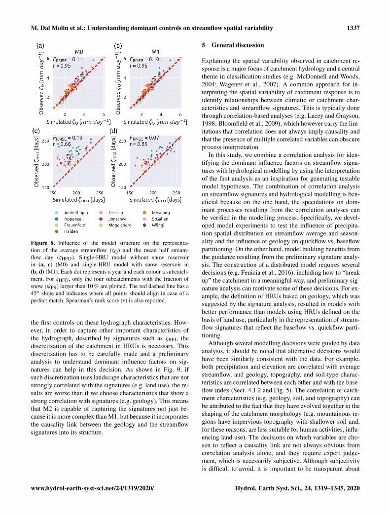
Figure 8 compares the ability of M0 and M1 to capture thesignatures representing average streamflow (ζQ) and season-ality (ζHFD). The analysis is presented for space–time valida-tion and, for ζHFD, focuses only on the four subcatchmentsthat are most affected by the snow (ψFS > 0.10), to empha-size the differences between the results of the two models.Each colour represents a different subcatchment and each dota year; the red dashed line has a 45◦ slope and representswhere the dots should align in case of perfect simulation re-sults. The normalized root mean square error and Spearman’srank score are also reported. It is important to stress that themodels have not been calibrated using any of the signaturesas an objective function, which therefore represent indepen-dent evaluation metrics.
It can be observed that M0 represents ζQ equally wellas M1, with almost no difference between the two models(r is 0.95 in both cases, whereas FRMSE is 0.11 for M0 and0.10 for M1). Focusing on the ability to capture ζHFD, it canbe seen that the points corresponding to M0 all lie in theupper-left part of the plot, meaning that this model under-estimates the signature values. With respect to M1, instead,the points are more aligned around the diagonal. This dif-ference in performance is captured by the values of FRMSE(0.13 for M0 and 0.07 for M1) and of r (0.66 for M0 and0.85 for M1).
Figure 9 compares the observed and simulated signaturesfor the other three models (M1, M2, and M3). All of themare equally good in representing ζQ (FRMSE is 0.10, 0.10,and 0.11, and r is 0.95, 0.96, and 0.95 for M1, M2, and M3respectively) and ζHFD (FRMSE is 0.07, 0.07, and 0.05 andr is 0.85, 0.84, and 0.87 for M1, M2, and M3 respectively).In all cases the cloud of points appears to be aligned to the di-agonal, meaning that the three models are able to capture thevalues of the signatures each year. Moreover, there is no sen-
M. Dal Molin et al.: Understanding dominant controls on streamflow spatial variability 1335
Figure 6. Spatial organization of the model structure: the catchment is divided into subcatchments (black lines), based on the location ofthe gauging stations, and HRUs (background colour), based on the catchment characteristics. All the HRUs have the same structure, buteach HRU has its own parameterization except for some shared parameters. In the case of a single-HRU model (i.e. M0 and M1), the modelmaintains the subdivision into subcatchments but loses the subdivision into multiple HRUs.
sible difference in the various models in representing thosesignatures.
The performance of all the models decreases for ζQ5 wherethe models have a similar performance, with FRMSE equalto 0.32, 0.28, and 0.33, and r equal to 0.62, 0.66, and 0.61 forM1, M2, and M3 respectively. The points are still alignedalong the diagonal but are quite dispersed, especially if com-pared with ζQ and ζHFD, meaning that the models capture thegeneral tendency but have deficiencies in capturing the inter-annual variability.
In terms of ζBFI, M2 performs clearly better than the othermodels. It is the only model that is able to represent thissignature, with FRMSE = 0.07, r = 0.83, and the points thatalign compactly with the diagonal. The other two modelshave a lower performance (FRMSE equal to 0.11 and 0.10, andr equal to 0.31 and 0.52 for M1 and M3 respectively), withpoints that are quite dispersed and align almost vertically,implying that the simulated values have a range of variabilitythat is definitely smaller than the observed data.
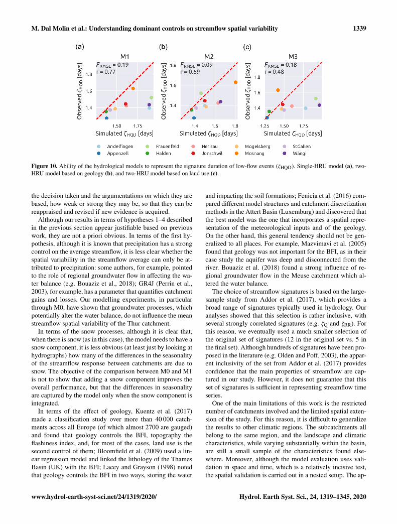
Figure 10 shows the comparison between observed andsimulated ζHQD; since this signature requires a long timewindow to be computed, it is not calculated year by year (asdone with the other signatures) but as an aggregated valueover the 24 years. In terms of performance, M2 still remains
the best among the three models, with FRMSE of 0.09 andr of 0.69; in second place comes M1, which outperforms M2in terms of r (0.77) but has a higher FRMSE (0.19), meaningthat M1 has the points that are more aligned but on a line thatis farther from the diagonal compared to M2; M3, finally, hasa bad performance, with high FRMSE (0.18) and low r (0.48).All the models tend to slightly overestimate the duration ofhigh-flow events with most of the points that lie on the right-hand side of the diagonal.
4.4 Hypotheses testing
The results of the hydrological model experiments appearto support our general hypothesis that only models that ac-count for the influence factors that affect the streamflow sig-natures are able to reproduce streamflow spatial variability(see Sect. 4.2.1). This provides confidence that those mod-els are a realistic representation of dominant processes in thecatchment.
The implications of the modelling results with respect tothe evaluation of the four hypotheses are explained as fol-lows.
1. Hypothesis 1: precipitation is the first driver of dif-ferences in the water balance. The good performanceof model M0 in the representation of the mean an-
1336 M. Dal Molin et al.: Understanding dominant controls on streamflow spatial variability
Figure 7. Normalized log likelihood (a) and Nash–Sutcliffe efficiency (b) for the three model configurations. (a) reports the variationbetween calibration and validation of the average of the 10 subcatchments; (b) shows the variation between subcatchments during space–time validation.
nual streamflow (ζQ) suggests that accounting for thespatial heterogeneity of the precipitation alone is suffi-cient to achieve a good representation of the annual wa-ter balance. More complex models, with more HRUs,processes, and parameters, while resulting in an over-all improvement of time series metrics, do not result inany improvement in simulating the water balance signa-ture ζQ.
2. Hypothesis 2: snow-related processes control differ-ences in streamflow seasonality. The improvement inthe representation of the streamflow seasonality ζHFDby M1 can be largely attributed to the (spatially vari-able) effect of snow accumulation and melting. Morecomplex models (M2 and M3) do not demonstrate animprovement in this signature, indicating that the struc-tural differences between these models do not have aninfluence on this signature.
3. Hypothesis 3: geology controls the partitioning betweenquickflow and baseflow. The ability of M2 to match
the signature ζBFI, which quantifies the separation be-tween quickflow and baseflow, much better than theother models, supports the hypothesis that geology hasa strong control on the partitioning between quickflowand baseflow. M2 is also the model with the average bestperformance in terms of streamflow metrics.
4. Hypothesis 4: characteristics that do not show correla-tions do not influence streamflow variability. The over-all lower performance of M3 compared to M2, in termsof both signatures and streamflow metrics, reassures usthat the relatively good results of M2 are not just due toincreasing complexity and confirms that adding charac-teristics that do not show correlations does not improvethe representation of spatial variability.
In summary, distributing the inputs in space and account-ing for the spatial distribution of snow-related processes aresufficient to get good performance metrics of water balanceand seasonality, confirming the fact that only the precipita-tion rate and the partitioning between rainfall and snow are
M. Dal Molin et al.: Understanding dominant controls on streamflow spatial variability 1337
Figure 8. Influence of the model structure on the representa-tion of the average streamflow (ζQ) and the mean half stream-flow day (ζHFD). Single-HRU model without snow reservoirin (a, c) (M0) and single-HRU model with snow reservoir in(b, d) (M1). Each dot represents a year and each colour a subcatch-ment. For ζHFD, only the four subcatchments with the fraction ofsnow (ψFS) larger than 10 % are plotted. The red dashed line has a45◦ slope and indicates where all points should align in case of aperfect match. Spearman’s rank score (r) is also reported.
the first controls on these hydrograph characteristics. How-ever, in order to capture other important characteristics ofthe hydrograph, described by signatures such as ζBFI, thediscretization of the catchment in HRUs is necessary. Thisdiscretization has to be carefully made and a preliminaryanalysis to understand dominant influence factors on sig-natures can help in this decision. As shown in Fig. 9, ifsuch discretization uses landscape characteristics that are notstrongly correlated with the signatures (e.g. land use), the re-sults are worse than if we choose characteristics that show astrong correlation with signatures (e.g. geology). This meansthat M2 is capable of capturing the signatures not just be-cause it is more complex than M1, but because it incorporatesthe causality link between the geology and the streamflowsignatures into its structure.
5 General discussion
Explaining the spatial variability observed in catchment re-sponse is a major focus of catchment hydrology and a centraltheme in classification studies (e.g. McDonnell and Woods,2004; Wagener et al., 2007). A common approach for in-terpreting the spatial variability of catchment response is toidentify relationships between climatic or catchment char-acteristics and streamflow signatures. This is typically donethrough correlation-based analyses (e.g. Lacey and Grayson,1998; Bloomfield et al., 2009), which however carry the lim-itations that correlation does not always imply causality andthat the presence of multiple correlated variables can obscureprocess interpretation.
In this study, we combine a correlation analysis for iden-tifying the dominant influence factors on streamflow signa-tures with hydrological modelling by using the interpretationof the first analysis as an inspiration for generating testablemodel hypotheses. The combination of correlation analysison streamflow signatures and hydrological modelling is ben-eficial because on the one hand, the speculations on dom-inant processes resulting from the correlation analyses canbe verified in the modelling process. Specifically, we devel-oped model experiments to test the influence of precipita-tion spatial distribution on streamflow average and season-ality and the influence of geology on quickflow vs. baseflowpartitioning. On the other hand, model building benefits fromthe guidance resulting from the preliminary signature analy-sis. The construction of a distributed model requires severaldecisions (e.g. Fenicia et al., 2016), including how to “breakup” the catchment in a meaningful way, and preliminary sig-nature analysis can motivate some of these decisions. For ex-ample, the definition of HRUs based on geology, which wassuggested by the signature analysis, resulted in models withbetter performance than models using HRUs defined on thebasis of land use, particularly in the representation of stream-flow signatures that reflect the baseflow vs. quickflow parti-tioning.
Although several modelling decisions were guided by dataanalysis, it should be noted that alternative decisions wouldhave been similarly consistent with the data. For example,both precipitation and elevation are correlated with averagestreamflow, and geology, topography, and soil-type charac-teristics are correlated between each other and with the base-flow index (Sect. 4.1.2 and Fig. 5). The correlation of catch-ment characteristics (e.g. geology, soil, and topography) canbe attributed to the fact that they have evolved together in theshaping of the catchment morphology (e.g. mountainous re-gions have impervious topography with shallower soil and,for these reasons, are less suitable for human activities, influ-encing land use). The decisions on which variables are cho-sen to reflect a causality link are not always obvious fromcorrelation analysis alone, and they require expert judge-ment, which is necessarily subjective. Although subjectivityis difficult to avoid, it is important to be transparent about
1338 M. Dal Molin et al.: Understanding dominant controls on streamflow spatial variability
Figure 9. Simulated vs. observed streamflow signatures. Single-HRU model on the left (M1), two-HRU model based on geology in thecentre (M2), and two-HRU model based on land use on the right (M3). Each dot represents a year and each colour a subcatchment. From upto bottom, mean daily streamflow (ζQ), baseflow index (ζBFI), mean half streamflow date (ζHFD, only the catchment with ψFS larger than10 %), and 5th percentile of the streamflow (ζQ5). The red dashed line has a 45◦ slope and indicates where all points should align in case ofa perfect match. Spearman’s rank score (r) is also reported.
M. Dal Molin et al.: Understanding dominant controls on streamflow spatial variability 1339
Figure 10. Ability of the hydrological models to represent the signature duration of low-flow events (ζHQD). Single-HRU model (a), two-HRU model based on geology (b), and two-HRU model based on land use (c).
the decision taken and the argumentations on which they arebased, how weak or strong they may be, so that they can bereappraised and revised if new evidence is acquired.
Although our results in terms of hypotheses 1–4 describedin the previous section appear justifiable based on previouswork, they are not a priori obvious. In terms of the first hy-pothesis, although it is known that precipitation has a strongcontrol on the average streamflow, it is less clear whether thespatial variability in the streamflow average can only be at-tributed to precipitation: some authors, for example, pointedto the role of regional groundwater flow in affecting the wa-ter balance (e.g. Bouaziz et al., 2018); GR4J (Perrin et al.,2003), for example, has a parameter that quantifies catchmentgains and losses. Our modelling experiments, in particularthrough M0, have shown that groundwater processes, whichpotentially alter the water balance, do not influence the meanstreamflow spatial variability of the Thur catchment.
In terms of the snow processes, although it is clear that,when there is snow (as in this case), the model needs to have asnow component, it is less obvious (at least just by looking athydrographs) how many of the differences in the seasonalityof the streamflow response between catchments are due tosnow. The objective of the comparison between M0 and M1is not to show that adding a snow component improves theoverall performance, but that the differences in seasonalityare captured by the model only when the snow component isintegrated.
In terms of the effect of geology, Kuentz et al. (2017)made a classification study over more than 40 000 catch-ments across all Europe (of which almost 2700 are gauged)and found that geology controls the BFI, topography theflashiness index, and, for most of the cases, land use is thesecond control of them; Bloomfield et al. (2009) used a lin-ear regression model and linked the lithology of the ThamesBasin (UK) with the BFI; Lacey and Grayson (1998) notedthat geology controls the BFI in two ways, storing the water
and impacting the soil formations; Fenicia et al. (2016) com-pared different model structures and catchment discretizationmethods in the Attert Basin (Luxemburg) and discovered thatthe best model was the one that incorporates a spatial repre-sentation of the meteorological inputs and of the geology.On the other hand, this general tendency should not be gen-eralized to all places. For example, Mazvimavi et al. (2005)found that geology was not important for the BFI, as in theircase study the aquifer was deep and disconnected from theriver. Bouaziz et al. (2018) found a strong influence of re-gional groundwater flow in the Meuse catchment which al-tered the water balance.
The choice of streamflow signatures is based on the large-sample study from Addor et al. (2017), which provides abroad range of signatures typically used in hydrology. Ouranalyses showed that this selection is rather inclusive, withseveral strongly correlated signatures (e.g. ζQ and ζRR). Forthis reason, we eventually used a much smaller selection ofthe original set of signatures (12 in the original set vs. 5 inthe final set). Although hundreds of signatures have been pro-posed in the literature (e.g. Olden and Poff, 2003), the appar-ent inclusivity of the set from Addor et al. (2017) providesconfidence that the main properties of streamflow are cap-tured in our study. However, it does not guarantee that thisset of signatures is sufficient in representing streamflow timeseries.
One of the main limitations of this work is the restrictednumber of catchments involved and the limited spatial exten-sion of the study. For this reason, it is difficult to generalizethe results to other climatic regions. The subcatchments allbelong to the same region, and the landscape and climaticcharacteristics, while varying substantially within the basin,are still a small sample of the characteristics found else-where. Moreover, although the model evaluation uses vali-dation in space and time, which is a relatively incisive test,the spatial validation is carried out in a nested setup. The ap-
1340 M. Dal Molin et al.: Understanding dominant controls on streamflow spatial variability
plication of systematic model development strategies to otherplaces and scales, and spatial validation to entirely differentregions, is necessary to obtain more generalizable insights.
The small number of subcatchments involved in thisstudy (10) limits the range of viable methods for identi-fying relationships between landscape and climatic indicesand streamflow signatures (Sect. 3.1) to rather simple ap-proaches. In particular, our correlation analysis, although ac-counting for non-linearity, is limited to monotonic correla-tions between variables, and it is unable to identify otherforms of relationship, including the mutual interaction be-tween various influence factors. The usage of more advancedtechniques, including machine learning approaches such asrandom forest or clustering analyses, is most efficient whenlarger samples are available and could represent a more suit-able choice in these situations.
6 Conclusion
In this study, we presented the development process of a dis-tributed model where model hypotheses, instead of beingmade a priori, are informed by preliminary analysis on de-termining the dominant climatic and landscape controls onstreamflow spatial variability. Besides providing guidance tomodel development, the proposed approach is useful in thefact that modelling can be used to test specific hypotheses ondominant processes resulting from such preliminary analysis.Our analysis was applied to the Thur catchment, subdividedinto 10 subcatchments based on available stream gauging sta-tions. The main findings are summarized in the followingpoints.
1. We found large spatial variability between the subcatch-ments of the Thur in terms of various streamflow sig-natures reflecting multiple temporal scales: yearly, sea-sonal, and event scale. In terms of climatic characteris-tics, indices reflecting fraction of snow, precipitation to-tals, and aridity varied considerably among catchments.Other precipitation characteristics such as season, fre-quency, and duration of dry and wet days did not varysignificantly among catchments. In terms of landscapecharacteristics, there is large variability of topography(e.g. from upstream mountainous to downstream flat ar-eas), geology (with unconsolidated, more permeable,and consolidated, relatively impermeable formations),and soils (with low depths in the mountains and largedepths in the floodplains) in all the catchments.
2. Based on correlation analysis and expert judgement, wedetermined that climatic variables, especially the pre-cipitation average, are the main controls on streamflowaverage yearly values; the fraction of snow is responsi-ble for streamflow seasonality by delaying the release ofwinter precipitation to the spring season, and geology
controls the baseflow index, with a higher fraction ofunconsolidated material determining higher baseflow.
3. The results of the signature analysis were translated intoa set of model hypotheses: a model with uniform param-eters and distributed precipitation input (M0), the addi-tion of a snow component (M1), the subdivision of thecatchment into geology-based HRUs (M2), and the al-ternative subdivision of the catchment using land-use-based HRUs (M3).
4. Using model comparison and a validation approach thatconsiders model performance (also in terms of signa-tures) in space–time validation, we found that it is nec-essary to account for the heterogeneity of precipitation,snow-related processes, and landscape features such asgeology in order to produce hydrographs that have sig-natures similar to the observed ones. In particular, weconfirmed that M0, in spite of a generally poor perfor-mance, is sufficient to capture signatures of streamflowaverage, showing that only distributing the meteorolog-ical inputs is sufficient to explain regional differencesin average streamflow and that other phenomena poten-tially altering the water balance (e.g. regional ground-water flows) do not play a significant role. M1 improvessignatures of streamflow seasonality, showing that snowis the main cause of the variability of the seasonalityamong the catchments. M2 enables signatures such asthe baseflow index to be reproduced, showing that in-corporating the geology of the catchment is importantfor reproducing regional differences in baseflow. Modelmodifications that are not in line with the results ofthe signature analysis, such as subdividing the catch-ment using land-use-based HRUs (M3), despite lead-ing to the same complexity as M2, cause deteriorationin model performance in space–time validation. Over-all, these results confirm the hypotheses based on thesignature analysis and suggest that the causality rela-tionships, explaining the influence of climate and land-scape characteristics on streamflow signatures, can beconstructively used for distributed model building.
The relatively good performance obtained in space–time val-idation suggests that the proposed approach could be usedfor the prediction of the streamflow in other ungauged loca-tions within the Thur catchment. The method proposed usesdata that are commonly available in many gauged catchments(e.g. meteorological data, streamflow measurements, maps ofelevation, geology, land use, and soil); therefore, it is easilytransferable to other locations.
M. Dal Molin et al.: Understanding dominant controls on streamflow spatial variability 1341
Appendix A: Hydrological model details
Model equations
The equations of the model are listed in this Appendix; themodel structure in presented in Fig. 6. Table A1 contains themodel parameters with the range of variability used in cal-ibration, Table A2 lists the water-budget equations, and Ta-bles A3 and A4 present the functions and the constitutivefunctions used.
Table A1. Hydrological model parameters with the range of variation used for the definition of the uniform prior distribution. The “compo-nent” column indicates the element (reservoir, lag, or network) where the parameter belongs.
Parameter Unit Component Range ofvariability
Ce – Unsaturated reservoir (UR) 0.1–3.0SUR
max mm Unsaturated reservoir (UR) 0.1–500.0kWR d−1 Snow reservoir (WR) 0.1–10.0t ILrise d Network lag 0.5–10.0tOLrise d Network lag 0.5–10.0D – Structure 0.0–1.0kFR d−1 mm−2 Fast reservoir (FR) 10−6–10.0kSR d−1 Slow reservoir (SR) 10−6–1.0tlagrise d Structure lag 1.0–20.0
Table A2. Water-budget equations (see the model schematic in Fig. 6).
(a) This equation is smoothed using a logistic scheme, Eq. (8) in Kavetski and Kuczera (2007), with smoothing parameter mP = 1.5 ◦C. (b) Thisequation is smoothed using a logistic scheme, Eq. (13) in Kavetski and Kuczera (2007), with smoothing parameter mM = 1.5 ◦C. (c) The operator ∗denotes the convolution operator, smoothed according to Kavetski and Kuczera (2007).
Table A4. Constitutive functions.
Function Name
fe(x|θ)= 1− exp(−x/θ) Tessier function. Note that fe(x|θ)→ 1 as x→∞.fp(x|θ)= x
θ Power functionfm(x|θ)=
x(1+θ)x+θ Monod-type kinetics, adjusted so that fm(1|θ)= 1
M. Dal Molin et al.: Understanding dominant controls on streamflow spatial variability 1343
Data availability. All the interpolated data used for this publi-cation as well as the codes to calculate the metrics (e.g. in-dices and signatures) are stored in an institutional repository(https://doi.org/10.25678/0001RK, Dal Molin et al., 2020). Dueto restrictions, the raw data have to be requested directly by theproviders. Meteorological data can be obtained by the FederalOffice of Meteorology and Climatology, MeteoSwiss; streamflowdata can be obtained from the Federal Office for the Environ-ment (FOEN); the maps used for calculating the catchments char-acteristics can be obtained by the Federal Office of Topography,swisstopo; all the other codes are available upon request.
Author contributions. MDM and FF designed all the experiments.MZ contributed to the preparation of the input data for the study.MDM conducted all the experiments and analysed the results.MDM prepared the paper with the contributions from all the au-thors.
Competing interests. The authors declare that they have no conflictof interest.
Special issue statement. This article is part of the special issue“Linking landscape organisation and hydrological functioning:from hypotheses and observations to concepts, models and under-standing (HESS/ESSD inter-journal SI)”. It is not associated with aconference.
Acknowledgements. The authors thank the Federal Office of Me-teorology and Climatology, MeteoSwiss, for the meteorologicaldata and the Federal Office for the Environment, FOEN, forthe streamflow data. The authors thank Conrad Jackisch (editor),Lieke Melsen, Shervan Gharari, and the two anonymous refereesfor their feedback and their help in improving this paper. MZ andMS dedicate this work to the memory of Joachim Gurtz, who pio-neered the work on distributed hydrological modelling in the Thurcatchment (Gurtz et al., 1999).
Financial support. This research has been supported bythe Schweizerischer Nationalfonds zur Förderung der Wis-senschaftlichen Forschung (grant no. 200021_169003).
Review statement. This paper was edited by Conrad Jackisch andreviewed by Lieke Melsen, Shervan Gharari, and two anonymousreferees.
References
Abbaspour, K. C., Yang, J., Maximov, I., Siber, R., Bogner,K., Mieleitner, J., Zobrist, J., and Srinivasan, R.: Mod-elling hydrology and water quality in the pre-alpine/alpine
Thur watershed using SWAT, J. Hydrol., 333, 413–430,https://doi.org/10.1016/j.jhydrol.2006.09.014, 2007.
Addor, N., Newman, A. J., Mizukami, N., and Clark, M. P.: TheCAMELS data set: catchment attributes and meteorology forlarge-sample studies, Hydrol. Earth Syst. Sci., 21, 5293–5313,https://doi.org/10.5194/hess-21-5293-2017, 2017.
Ajami, K. N., Gupta, H., Wagener, T., and Sorooshian, S.: Cal-ibration of a semi-distributed hydrologic model for stream-flow estimation along a river system, J. Hydrol., 298, 112–135,https://doi.org/10.1016/j.jhydrol.2004.03.033, 2004.
Andréassian, V., Perrin, C., Berthet, L., Le Moine, N., Lerat, J.,Loumagne, C., Oudin, L., Mathevet, T., Ramos, M. H., andValéry, A.: HESS Opinions “Crash tests for a standardized eval-uation of hydrological models”, Hydrol. Earth Syst. Sci., 13,1757–1764, https://doi.org/10.5194/hess-13-1757-2009, 2009.
Antonetti, M. and Zappa, M.: How can expert knowledge in-crease the realism of conceptual hydrological models? A casestudy based on the concept of dominant runoff process inthe Swiss Pre-Alps, Hydrol. Earth Syst. Sci., 22, 4425–4447,https://doi.org/10.5194/hess-22-4425-2018, 2018.
Antonetti, M., Buss, R., Scherrer, S., Margreth, M., and Zappa,M.: Mapping dominant runoff processes: an evaluation ofdifferent approaches using similarity measures and syntheticrunoff simulations, Hydrol. Earth Syst. Sci., 20, 2929–2945,https://doi.org/10.5194/hess-20-2929-2016, 2016.
Arnold, J. G., Srinivasan, R., Muttiah, R. S., and Williams, J.R.: Large Area Hydrologic Modeling And Assessment Part I:Model Development, J. Am. Water Resour. Assoc., 34, 73–89,https://doi.org/10.1111/j.1752-1688.1998.tb05961.x, 1998.
Berger, K. P. and Entekhabi, D.: Basin hydrologic response relationsto distributed physiographic descriptors and climate, J. Hydrol.,247, 169–182, https://doi.org/10.1016/S0022-1694(01)00383-3,2001.
Bloomfield, J. P., Allen, D. J., and Griffiths, K. J.: Examining geo-logical controls on baseflow index (BFI) using regression analy-sis: An illustration from the Thames Basin, UK, J. Hydrol., 373,164–176, https://doi.org/10.1016/j.jhydrol.2009.04.025, 2009.
Bouaziz, L., Weerts, A., Schellekens, J., Sprokkereef, E., Stam,J., Savenije, H., and Hrachowitz, M.: Redressing the balance:quantifying net intercatchment groundwater flows, Hydrol. EarthSyst. Sci., 22, 6415–6434, https://doi.org/10.5194/hess-22-6415-2018, 2018.
Box, G. E. P. and Cox, D. R.: An Analysis of Transformations, J.Roy. Stat. Soc. B, 26, 211–252, 1964.
Boyle, D. P., Gupta, H. V., Sorooshian, S., Koren, V., Zhang, Z.,and Smith, M.: Toward improved streamflow forecasts: value ofsemidistributed modeling, Water Resour. Res., 37, 2749–2759,https://doi.org/10.1029/2000wr000207, 2001.
Brunner, M. I., Furrer, R., and Favre, A. C.: Modeling the spa-tial dependence of floods using the Fisher copula, Hydrol.Earth Syst. Sci., 23, 107–124, https://doi.org/10.5194/hess-23-107-2019, 2019.
Court, A.: Measures of streamflow timing, J. Geophys. Res., 67,4335–4339, https://doi.org/10.1029/JZ067i011p04335, 1962.
Dal Molin, M., Schirmer, M., Zappa, M., and Fenicia, F.: Datafor: Understanding dominant controls on streamflow spatialvariability to set-up a semi-distributed hydrological model:the case study of the Thur catchment, [Data set], Eawag:
1344 M. Dal Molin et al.: Understanding dominant controls on streamflow spatial variability
Swiss Federal Institute of Aquatic Science and Technology,https://doi.org/10.25678/0001RK, 2020.
De Lavenne, A., Thirel, G., Andréassian, V., Perrin, C., and Ramos,M.-H.: Spatial variability of the parameters of a semi-distributedhydrological model, in: 7th International Water Resources Man-agement Conference of ICWRS, 18–20 May 2016, Bochum,Germany, 87–94, 2016.
Falkenmark, M. and Chapman, T.: Comparative hydrology: An eco-logical approach to land and water resources, The Unesco Press,, 1989.
Fenicia, F., Kavetski, D., and Savenije, H. H. G.: Elements of aflexible approach for conceptual hydrological modeling: 1. Mo-tivation and theoretical development, Water Resour. Res., 47,W11510, https://doi.org/10.1029/2010wr010174, 2011.
Fenicia, F., Kavetski, D., Savenije, H. H. G., Clark, M. P., Schoups,G., Pfister, L., and Freer, J.: Catchment properties, function, andconceptual model representation: is there a correspondence?, Hy-drol. Process., 28, 2451–2467, https://doi.org/10.1002/hyp.9726,2014.
Fenicia, F., Kavetski, D., Savenije, H. H. G., and Pfister, L.: Fromspatially variable streamflow to distributed hydrological mod-els: Analysis of key modeling decisions, Water Resour. Res., 52,954–989, https://doi.org/10.1002/2015wr017398, 2016.
Feyen, L., Kalas, M., and Vrugt, J. A.: Semi-distributed param-eter optimization and uncertainty assessment for large-scalestreamflow simulation using global optimization/Optimisation deparamètres semi-distribués et évaluation de l’incertitude pour lasimulation de débits à grande échelle par l’utilisation d’une opti-misation globale, Hydrolog. Sci. J., 53, 293–308, 2008.
Fundel, F., Jorg-Hess, S., and Zappa, M.: Monthly hydrometeoro-logical ensemble prediction of streamflow droughts and corre-sponding drought indices, Hydrol. Earth Syst. Sci., 17, 395–407,https://doi.org/10.5194/hess-17-395-2013, 2013.
Gao, H., Hrachowitz, M., Fenicia, F., Gharari, S., and Savenije,H. H. G.: Testing the realism of a topography-drivenmodel (FLEX-Topo) in the nested catchments of the Up-per Heihe, China, Hydrol. Earth Syst. Sci., 18, 1895–1915,https://doi.org/10.5194/hess-18-1895-2014, 2014.
Garen, D. C. and Marks, D.: Spatial fields of meteorological in-put data including forest canopy corrections for an energy bud-get snow simulation model, Proceedings of a symposium heldduring the Sixth IAHS Scientific Assembly at Maastricht, TheNetherlands, July 2001, IAHS Publ. no. 270, 349–354, 2001.
Gurtz, J., Baltensweiler, A., and Lang, H.: Spatially dis-tributed hydrotope-based modelling of evapotranspira-tion and runoff in mountainous basins, Hydrol. Pro-cess., 13, 2751–2768, https://doi.org/10.1002/(Sici)1099-1085(19991215)13:17<2751::Aid-Hyp897>3.3.Co;2-F, 1999.
Gurtz, J., Verbunt, M., Zappa, M., Moesch, M., Pos, F., andMoser, U.: Long-term hydrometeorological measurements andmodel-based analyses in the hydrological research catchment Ri-etholzbach, J. Hydrol. Hydromech., 51, 162–174, 2003.
Hrachowitz, M., Savenije, H., Blöschl, G., McDonnell, J., Siva-palan, M., Pomeroy, J., Arheimer, B., Blume, T., Clark, M., andEhret, U.: A decade of Predictions in Ungauged Basins (PUB) –a review, Hydrolog. Sci. J., 58, 1198–1255, 2013.
Jasper, K., Calanca, P., Gyalistras, D., and Fuhrer, J.: Dif-ferential impacts of climate change on the hydrology
of two alpine river basins, Clim. Res., 26, 113–129,https://doi.org/10.3354/cr026113, 2004.
Jorg-Hess, S., Kempf, S. B., Fundel, F., and Zappa, M.: The bene-fit of climatological and calibrated reforecast data for simulatinghydrological droughts in Switzerland, Meteorol. Appl., 22, 444–458, https://doi.org/10.1002/met.1474, 2015.
Kavetski, D. and Kuczera, G.: Model smoothing strategies to re-move microscale discontinuities and spurious secondary optimain objective functions in hydrological calibration, Water Resour.Res., 43, W03411, https://doi.org/10.1029/2006wr005195, 2007.
Kavetski, D., Kuczera, G., Thyer, M., and Renard, B.: MultistartNewton-type optimisation methods for the calibration of con-ceptual hydrological models, in: Modsim 2007: InternationalCongress on Modelling and Simulation, December 2007 Uni-versity of Canterbury, Christchurch, New Zealand, 2513–2519,2007.
Kavetski, D., Fenicia, F., and Clark, M. P.: Impact of tempo-ral data resolution on parameter inference and model iden-tification in conceptual hydrological modeling: Insights froman experimental catchment, Water Resour. Res., 47, W05501,https://doi.org/10.1029/2010wr009525, 2011.
Kirchner, J. W., Feng, X. H., Neal, C., and Robson, A. J.:The fine structure of water-quality dynamics: the (high-frequency) wave of the future, Hydrol. Process., 18, 1353–1359,https://doi.org/10.1002/hyp.5537, 2004.
Kroll, C. N. and Song, P.: Impact of multicollinearity on small sam-ple hydrologic regression models, Water Resour. Res., 49, 3756–3769, https://doi.org/10.1002/wrcr.20315, 2013.
Kuentz, A., Arheimer, B., Hundecha, Y., and Wagener, T.: Un-derstanding hydrologic variability across Europe through catch-ment classification, Hydrol. Earth Syst. Sci., 21, 2863–2879,https://doi.org/10.5194/hess-21-2863-2017, 2017.
Lacey, G. C. and Grayson, R. B.: Relating baseflow to catchmentproperties in south-eastern Australia, J. Hydrol., 204, 231–250,https://doi.org/10.1016/S0022-1694(97)00124-8, 1998.
Ladson, A. R., Brown, R., Neal, B., and Nathan, R.: A StandardApproach to Baseflow Separation Using The Lyne and HollickFilter, Aust. J. Water Resour., 17, 25–34, 2013.
Lerat, J., Andreassian, V., Perrin, C., Vaze, J., Perraud, J.-M., Rib-stein, P., and Loumagne, C.: Do internal flow measurements im-prove the calibration of rainfall-runoff models?, Water Resour.Res., 48, W02511, https://doi.org/10.1029/2010WR010179,2012.
Lindstrom, G., Johansson, B., Persson, M., Gardelin, M., andBergstrom, S.: Development and test of the distributedHBV-96 hydrological model, J. Hydrol., 201, 272–288,https://doi.org/10.1016/S0022-1694(97)00041-3, 1997.
Mazvimavi, D., Meijerink, A. M. J., Savenije, H. H. G., and Stein,A.: Prediction of flow characteristics using multiple regressionand neural networks: A case study in Zimbabwe, Phys. Chem.Earth, 30, 639–647, https://doi.org/10.1016/j.pce.2005.08.003,2005.
McDonnell, J. J. and Woods, R.: On the need for catchment classi-fication, J. Hydrol., 299, 2–3, 2004.
McInerney, D., Thyer, M., Kavetski, D., Lerat, J., and Kucz-era, G.: Improving probabilistic prediction of daily streamflowby identifying Pareto optimal approaches for modeling het-eroscedastic residual errors, Water Resour. Res., 53, 2199–2239,https://doi.org/10.1002/2016wr019168, 2017.
M. Dal Molin et al.: Understanding dominant controls on streamflow spatial variability 1345
McInerney, D., Thyer, M., Kavetski, D., Githui, F., Thayalaku-maran, T., Liu, M., and Kuczera, G.: The Importance of Spa-tiotemporal Variability in Irrigation Inputs for HydrologicalModeling of Irrigated Catchments, Water Resour. Res., 54,6792–6821, https://doi.org/10.1029/2017wr022049, 2018.
Melsen, L., Teuling, A., Torfs, P., Zappa, M., Mizukami, N., Clark,M., and Uijlenhoet, R.: Representation of spatial and temporalvariability in large-domain hydrological models: case study for amesoscale pre-Alpine basin, Hydrol. Earth Syst. Sci., 20, 2207–2226, https://doi.org/10.5194/hess-20-2207-2016, 2016.
Melsen, L. A., Teuling, A. J., van Berkum, S. W., Torfs, P. J. J.F., and Uijlenhoet, R.: Catchments as simple dynamical sys-tems: A case study on methods and data requirements forparameter identification, Water Resour. Res., 50, 5577–5596,https://doi.org/10.1002/2013WR014720, 2014.
Menzel, L.: Modelling canopy resistances and transpi-ration of grassland, Phys. Chem. Earth, 21, 123–129,https://doi.org/10.1016/S0079-1946(97)85572-3, 1996.
Monteith, J. L.: Vegetation and the atmosphere, Academic Press,London, New York, 1975.
Olden, J. D. and Poff, N. L.: Redundancy and the choice of hydro-logic indices for characterizing streamflow regimes, River Res.Appl., 19, 101–121, https://doi.org/10.1002/rra.700, 2003.
Parajka, J., Merz, R., and Blöschl, G.: A comparison of regionali-sation methods for catchment model parameters, Hydrol. EarthSyst. Sci., 9, 157–171, https://doi.org/10.5194/hess-9-157-2005,2005.
Perrin, C., Michel, C., and Andréassian, V.: Improvement of a parsi-monious model for streamflow simulation, J. Hydrol., 279, 275–289, https://doi.org/10.1016/S0022-1694(03)00225-7, 2003.
Sawicz, K., Wagener, T., Sivapalan, M., Troch, P. A., andCarrillo, G.: Catchment classification: empirical analysis ofhydrologic similarity based on catchment function in theeastern USA, Hydrol. Earth Syst. Sci., 15, 2895–2911,https://doi.org/10.5194/hess-15-2895-2011, 2011.
Scherrer, S. and Naef, F.: A decision scheme to indicate dominanthydrological flow processes on temperate grassland, Hydrol. Pro-cess., 17, 391–401, https://doi.org/10.1002/hyp.1131, 2003.
Schirmer, M., Luster, J., Linde, N., Perona, P., Mitchell, E. A. D.,Barry, D. A., Hollender, J., Cirpka, O. A., Schneider, P., Vogt,T., Radny, D., and Durisch-Kaiser, E.: Morphological, hydrolog-ical, biogeochemical and ecological changes and challenges inriver restoration – the Thur River case study, Hydrol. Earth Syst.Sci., 18, 2449–2462, https://doi.org/10.5194/hess-18-2449-2014,2014.
Seneviratne, S. I., Lehner, I., Gurtz, J., Teuling, A. J., Lang, H.,Moser, U., Grebner, D., Menzel, L., Schroff, K., Vitvar, T., andZappa, M.: Swiss prealpine Rietholzbach research catchment andlysimeter: 32 year time series and 2003 drought event, Water Re-sour. Res., 48, W06526, https://doi.org/10.1029/2011wr011749,2012.
Sivapalan, M.: Pattern, Process and Function: Elements of a Uni-fied Theory of Hydrology at the Catchment Scale, in: Encyclo-pedia of Hydrological Sciences, edited by: Anderson, M. G. andMcDonnell, J. J., https://doi.org/10.1002/0470848944.hsa012,2006.
Toth, E.: Catchment classification based on characterisation ofstreamflow and precipitation time series, Hydrol. Earth Syst.Sci., 17, 1149–1159, https://doi.org/10.5194/hess-17-1149-2013,2013.
Trancoso, R., Phinn, S., McVicar, T. R., Larsen, J. R., andMcAlpine, C. A.: Regional variation in streamflow driversacross a continental climatic gradient, Ecohydrology, 10, e1816,https://doi.org/10.1002/eco.1816, 2017.
van Esse, W. R., Perrin, C., Booij, M. J., Augustijn, D. C. M., Feni-cia, F., Kavetski, D., and Lobligeois, F.: The influence of concep-tual model structure on model performance: a comparative studyfor 237 French catchments, Hydrol. Earth Syst. Sci., 17, 4227–4239, https://doi.org/10.5194/hess-17-4227-2013, 2013.
Verbunt, M., Zappa, M., Gurtz, J., and Kaufmann, P.: Verifica-tion of a coupled hydrometeorological modelling approach foralpine tributaries in the Rhine basin, J. Hydrol., 324, 224–238,https://doi.org/10.1016/j.jhydrol.2005.09.036, 2006.
Viviroli, D., Zappa, M., Gurtz, J., and Weingartner, R.: An introduc-tion to the hydrological modelling system PREVAH and its pre-and post-processing-tools, Environ. Model. Softw., 24, 1209–1222, https://doi.org/10.1016/j.envsoft.2009.04.001, 2009.
von Freyberg, J., Radny, D., Gall, H. E., and Schirmer, M.: Implica-tions of hydrologic connectivity between hillslopes and riparianzones on streamflow composition, J. Contam. Hydrol., 169, 62–74, https://doi.org/10.1016/j.jconhyd.2014.07.005, 2014.
von Freyberg, J., Moeck, C., and Schirmer, M.: Estima-tion of groundwater recharge and drought severity withvarying model complexity, J. Hydrol., 527, 844–857,https://doi.org/10.1016/j.jhydrol.2015.05.025, 2015.
Wagener, T., Boyle, D. P., Lees, M. J., Wheater, H. S., Gupta, H. V.,and Sorooshian, S.: A framework for development and applica-tion of hydrological models, Hydrol. Earth Syst. Sci., 5, 13–26,https://doi.org/10.5194/hess-5-13-2001, 2001.
Wagener, T., Sivapalan, M., McDonnell, J., Hooper, R., Lakshmi,V., Liang, X., and Kumar, P.: Predictions in ungauged basins asa catalyst for multidisciplinary hydrology, Eos Trans. Am. Geo-phys. Union, 85, 451–457, 2004.
Wagener, T., Sivapalan, M., Troch, P., and Woods, R.: Catch-ment Classification and Hydrologic Similarity, Geogr. Compass,1, 901–931, https://doi.org/10.1111/j.1749-8198.2007.00039.x,2007.
Wooldridge, S., Kalma, J., and Kuczera, G.: Parameterisationof a simple semi-distributed model for assessing the impactof land-use on hydrologic response, J. Hydrol., 254, 16–32,https://doi.org/10.1016/S0022-1694(01)00489-9, 2001.