Calhoun: The NPS Institutional Archive Theses and Dissertations Thesis Collection 1996-12 Predistortion of quadrature amplitude modulation signals using Volterra series approximation Donovan, Michael T. Monterey, California. Naval Postgraduate School http://hdl.handle.net/10945/31971
Transcript
Calhoun: The NPS Institutional Archive
Theses and Dissertations Thesis Collection
1996-12
Predistortion of quadrature amplitude modulation
signals using Volterra series approximation
Donovan, Michael T.
Monterey, California. Naval Postgraduate School
http://hdl.handle.net/10945/31971
NAVAL POSTGRADUATE SCHOOL Monterey, California
THESIS
·PREDISTORTION OF QUADRATURE AMPLITUDE MODULATION
SIGNALS USING VOL TERRA SERIES APPROXIMATION
by
Michael T. Donovan
December, 1996
Thesis Advisor: Murali Tummala
Approved for public release; distribution is unlimited.
Public reponing burden lor this collection of information IS estimated to aYerage 1 hOur per response. including the time reviewing instructions. searching existing data sources gathering and malmalnlng the data needed. and completing and reviewing the collection of information. Send commems regarding thiS burden estimate or any other aspect of this collection of informatiOn, Including suggestions lor reducing this burden to Washington Headquaners Services, Directorate lOr Information Operations and Reports. 1215 Jefferson DaYis HighWay, Sutte 1204, Arlington, VA 22202-4302, and to the Ollice of Managemem and Budget, Paperwork Reduction Project (0704·0188), Washington, DC 20503.
1. AGENCY USE ONLY CLeave Blank) 12. REPORT DATE 3. REPORT TYPE AND DATES COVERED
December 1996 Master's Thesis 4. TrTLE AND SUBTrTLE 5. FUNDING NUMBERS
PREDISTORTION OF QUADRATURE AMPLITUDE MODULATION SIGNALS USING VOLTERRA SERIES APPROXIMATION
6. AUTHOR(S)
Donovan, Michael T.
7. PERFORMING ORGANIZATION NAME(S) AND ADDRESS(ES) 8. PERFORMING ORGANIZATION
Naval Postgraduate School REPORT NUMBER
Monterey, CA 93943-5000
9. SPONSORING/ MONrTORING AGENCY NAME(S) AND ADDRESS(ES) 10. SPONSORING/ MONrTORING AGENCY REPORT NUMBER
11. SUPPLEMENTARY NOTES The views expressed in this thesis are those of the author and do not reflect the official policy or position of the Department of Defense or the United States Government.
12a. DISTRIBUTION I AVAILABILrTY STATEMENT 12b. DISTRIBUTION CODE
Approved for public release; distribution is unlimited
13. ABSTRACT (Maximum 200 words)
Modem digital communication systems are being called upon to move ever increasing amounts of information over
decreasingly available bandwidth. This requires that communication systems employ bandwidth-efficient modulation schemes
to conserve bandwidth while moving the information at higher data rates. A major stumbling block to using higher order
modulation schemes in long haul communication is the <fistortion caused by high power amplifiers. These high power
amplifiers are required to amplify the signal power to a level that will allow distant receivers to correctly demodulate and decode
the information. The distortion caused by the high power amplifiers can render a modulation scheme unusable due to the high
symbol error rates which result from the extensive skewing of the modulation scheme's signal constellation. This thesis details
a predistortion technique using Volterra series approximation techniques to model the inverse of the high power amplifier's
distortion characteristics. A 64 Quadrature Amplitude Modulation (64-QAM) system incorporating a predistorter is used to
demonstrate the ability to achieve acceptable bit error rates. The implementation of the inverse model and the communication
system is performed in MA1LAB. The results show the viability of predistortion of digital data to allow the higher order
modulation schemes to be incorporated into communication schemes, increasing the overall data rate while conserving
bandwidth.
14. SUBJECT TERMS High Data Rate Communications, QAM, Volterra Series, Predistortion
Standard Form 298 (Rev. 2-89) Prescribed by ANSI Std. 239-18
ii
Author:
Approved for public release; distribution is unlimited.
PREDISTORTION OF QUADRATURE AMPLITUDE MODULATION SIGNALS
USING VOLTERRA SERIES APPROXIMATION
Michael T. Donovan Major, United States Army
B.S., Purdue University, 1984
Submitted in partial fulfillment of the requirements for the degree of
MASTER OF SCIENCE IN ELECTRICAL ENGINEERING
from the
NAVAL POSTGRADUATE SCHOOL December 1996
Approved by: Murali Tummala, Thesis Advisor
Herschel H. Loomis, Jr., Ch:mn~n. Department of Electrical and Computer Engineering
DTIC QUtl.LI'l'Y II;J87EDTED 5'
111
iv
ABSTRACT
Modem digital communication systems are being called upon to move ever
increasing amounts of information over decreasingly available bandwidth. This requires
that communication systems employ bandwidth-efficient modulation schemes to conserve
bandwidth while moving the information at higher data rates. A major stumbling block to
using higher order modulation schemes in long haul communication is the distortion caused
by high power amplifiers. These high power amplifiers are required to amplify the signal
power to a level that will allow distant receivers to correctly demodulate and decode the
information. The distortion caused by the high power amplifiers can render a modulation
scheme unusable due to the high symbol error rates which result from the extensive
skewing of the modulation scheme's signal constellation. This thesis details a predistortion
technique using Volterra series approximation techniques to model the inverse of the high
power amplifier's distortion characteristics. A 64 Quadrature Amplitude Modulation (64-
QAM) system incorporating a predistorter is used to demonstrate the ability to achieve
acceptable bit error rates. The implementation of the inverse model and the communication
system is performed in MA TLAB. The results show the viability of predistortion of digital
data to allow the higher order modulation schemes to be incorporated into communication
schemes, increasing the overall data rate while conserving bandwidth.
v
vi
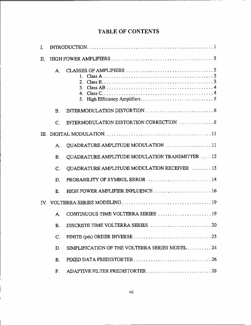
TABLE OF CONTENTS
I. IN"TRODUCTION .................................................... 1
II. HIGH POWER AMPLIFIERS .......................................... 3
A. CLASSES OF AMPLIFIERS .................................... 3 1. Class A ............................................. 3 2. Class B .............................................. 3 3. Class AB ............................................ 4 4. Class C .............................................. 4 5. High Efficiency Amplifiers .............................. 5
B. IN"TERMODULATIONDISTORTION ............................ 6
C. IN"TERMODULATION DISTORTION CORRECTION .............. 8
III. DIGITAL MODULATION ............................................ 11
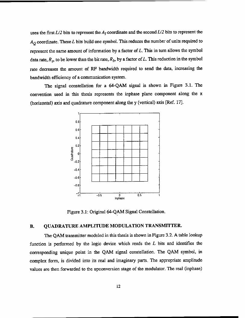
A. QUADRATURE AMPLITUDE MODULATION ................... 11
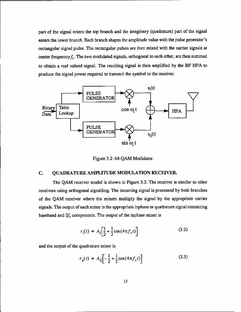
B. QUADRATURE AMPLITUDE MODULATION TRANSMITTER .... 12
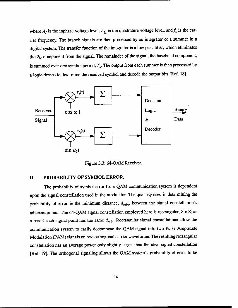
C. QUADRATURE AMPLITUDE MODULATION RECEIVER ........ 13
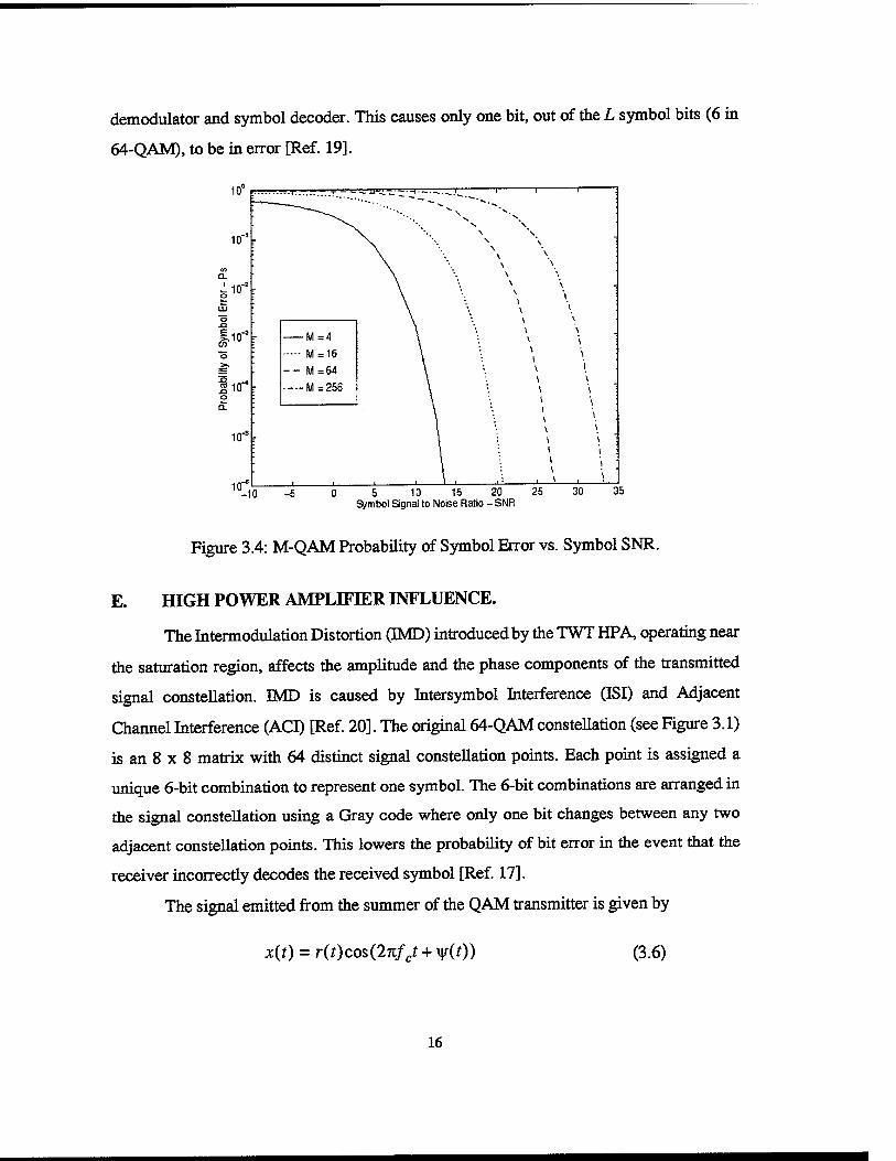
D. PROBABILITY OF SYMBOL ERROR .......................... 14
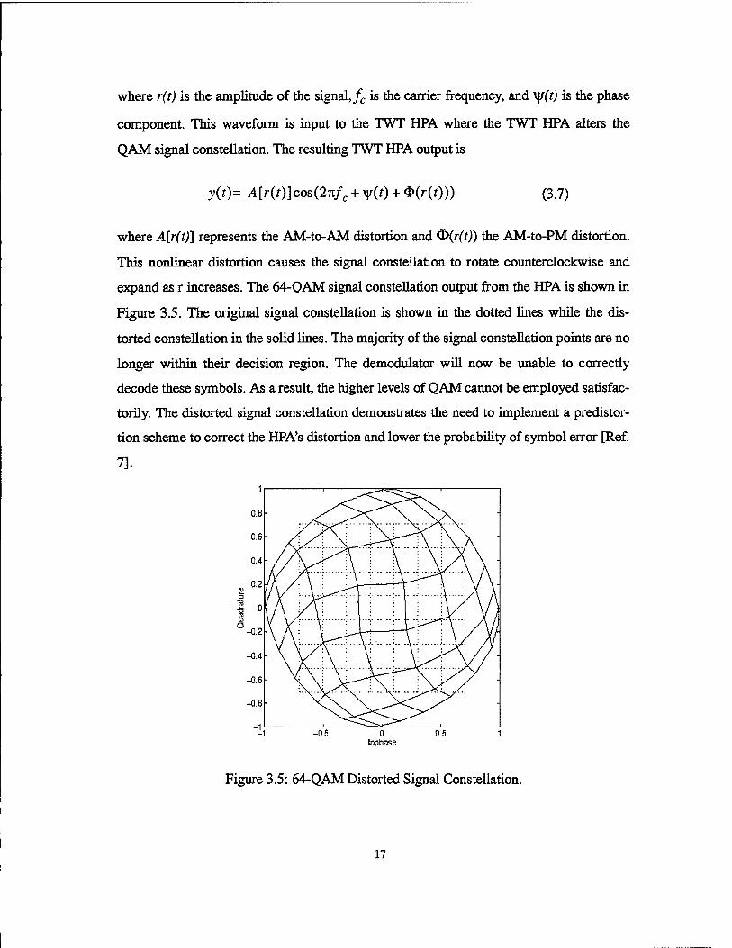
E. IDGH POWER AMPLIFIER INFLUENCE ........................ 16
IV. VOLTERRA SERIES MODELING ..................................... 19
A. CONTINUOUS TIME VOLTERRA SERIES ...................... 19
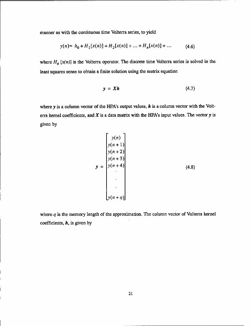
B. DISCRETE TIME VOLTERRA SERIES ......................... 20
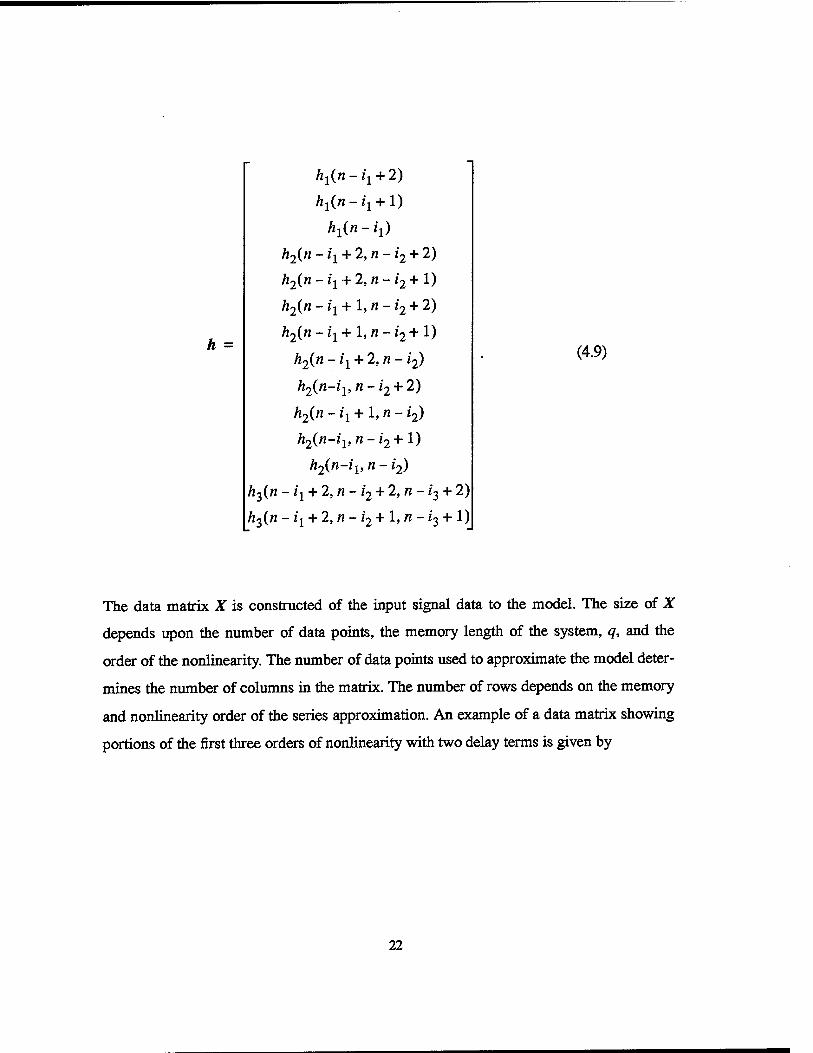
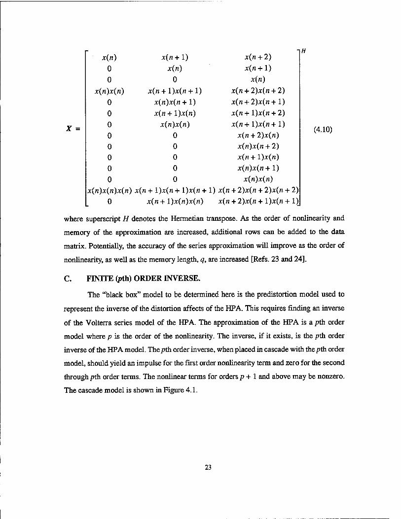
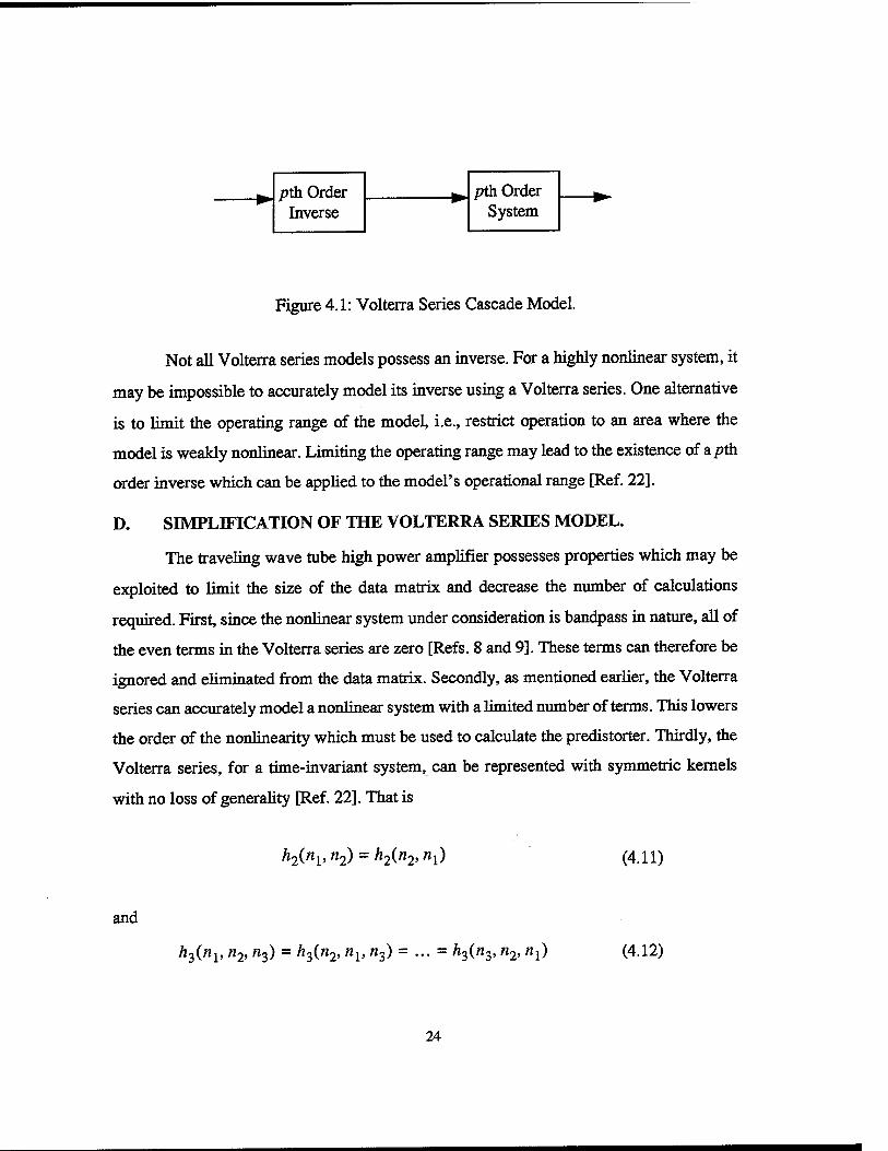
C. FINITE (pth) ORDER INVERSE ................................ 23
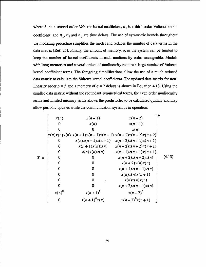
D. SIJviPLIFICATION OF THE VOLTERRA SERIES MODEL .......... 24
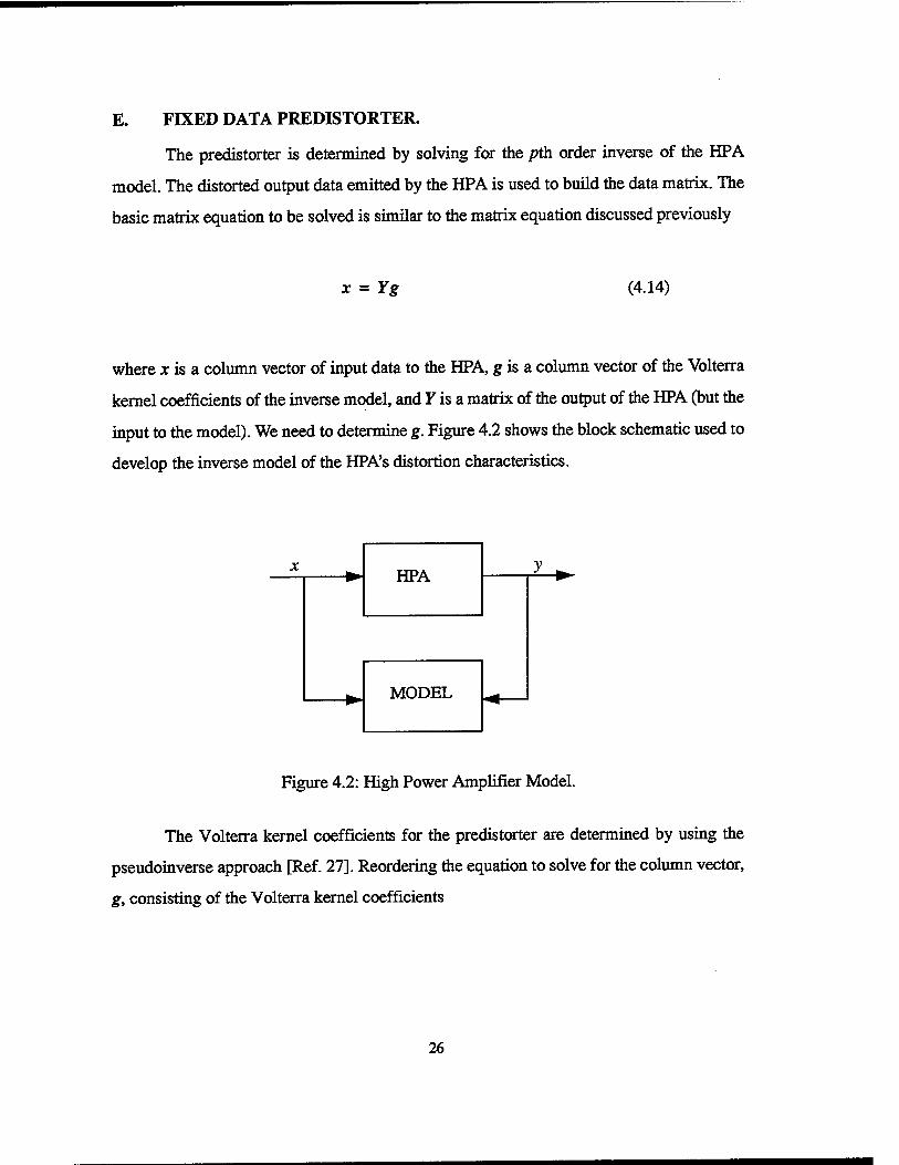
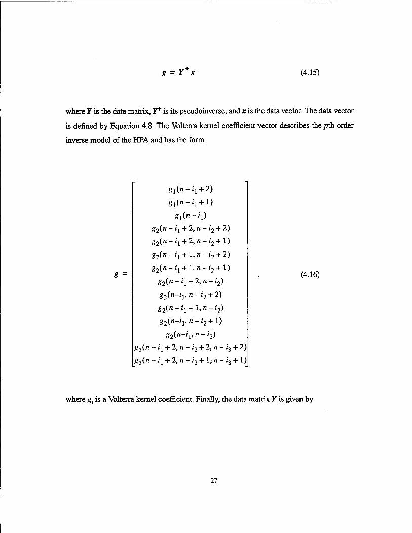
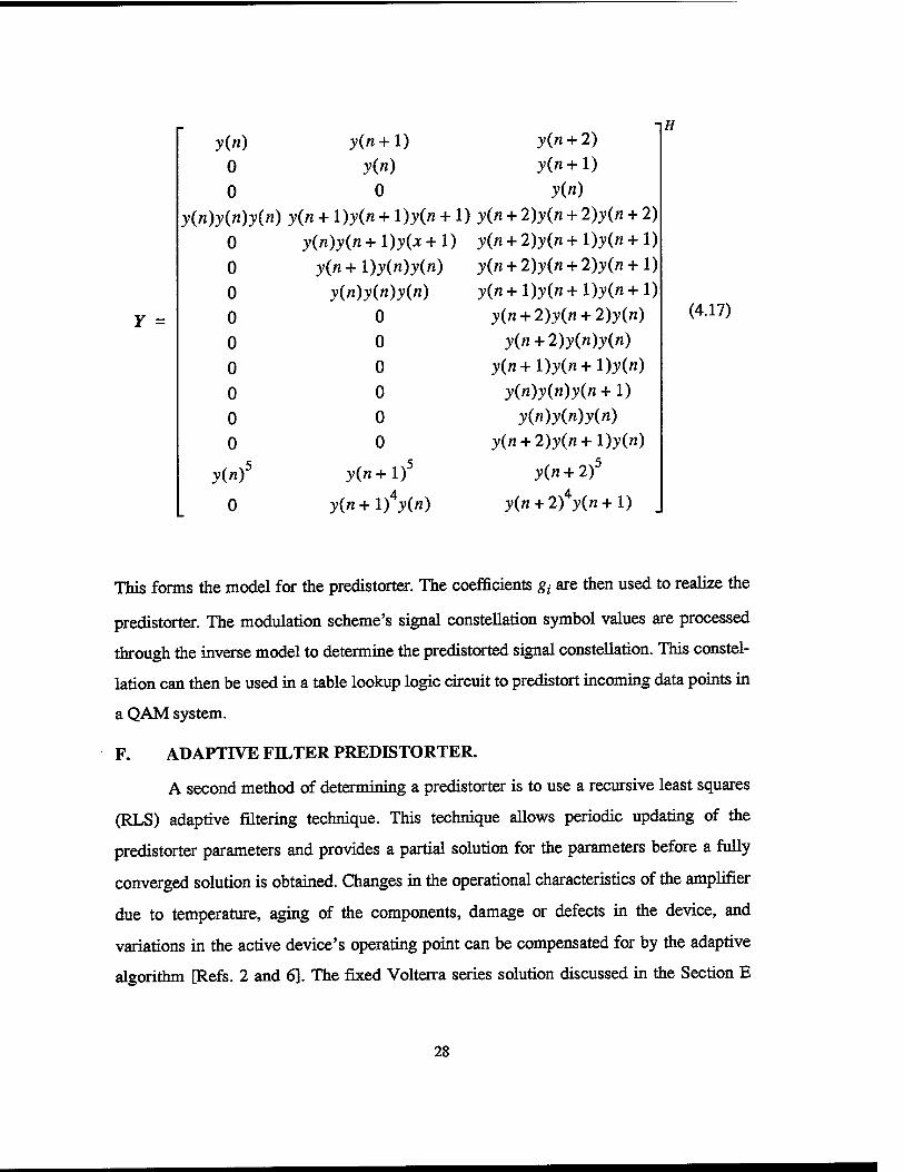
E. FIXED DATA PREDISTOR TER ................................ 26
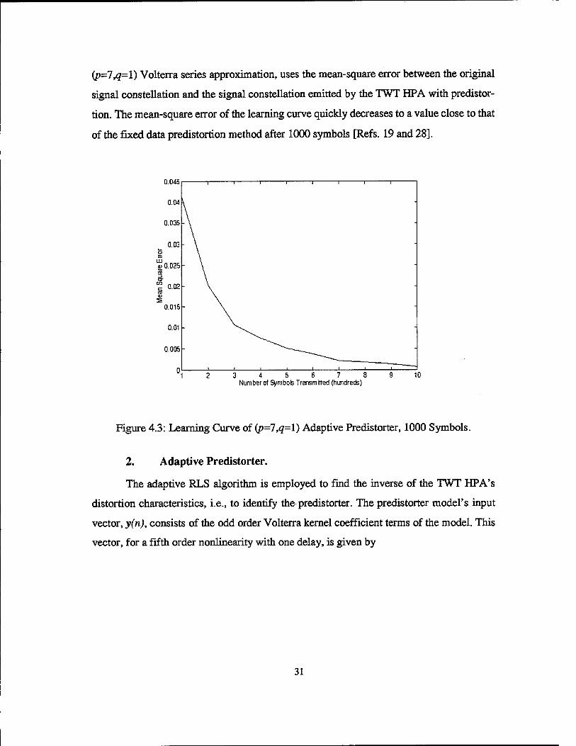
F. ADAPTIVE FILTER PREDISTORTER ........................... 28
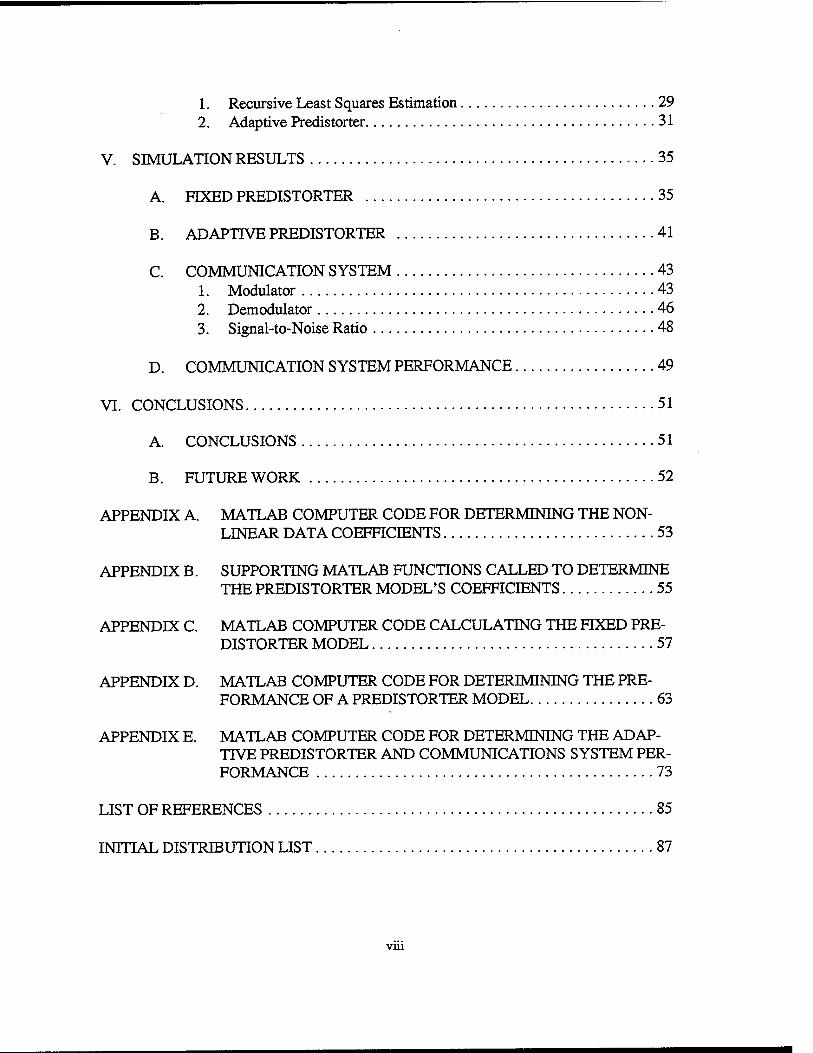
V. SIMULATION RESULTS ............................................ 35
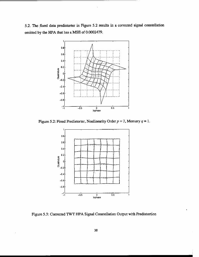
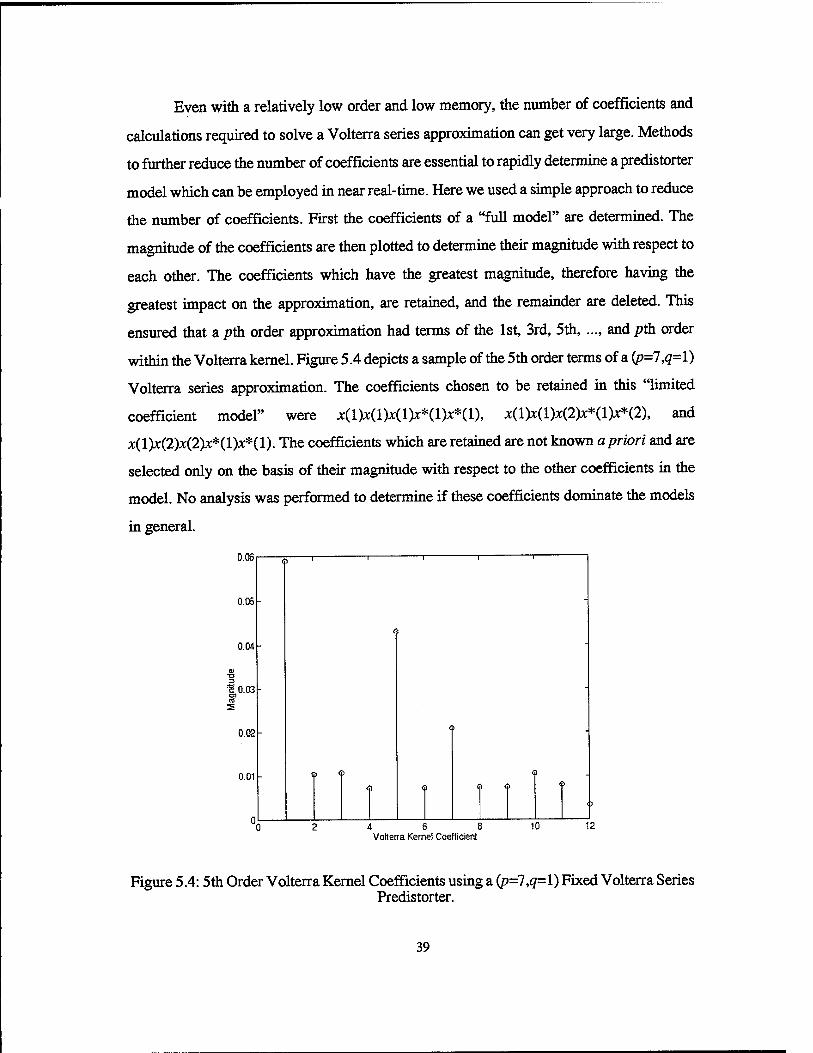
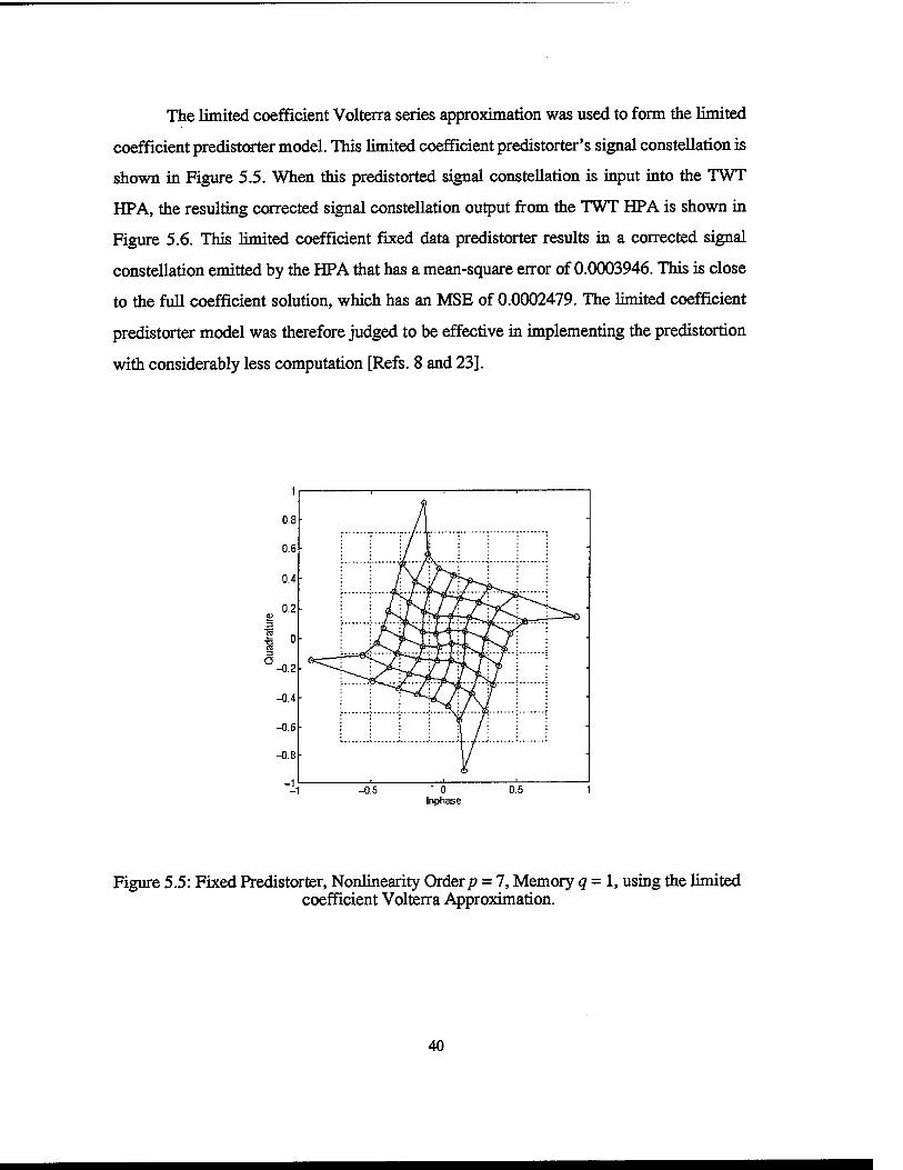
A. FIXED PREDISTORTER ..................................... 35
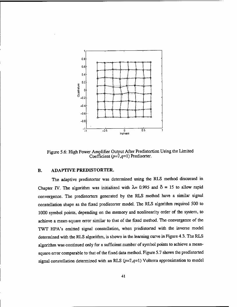
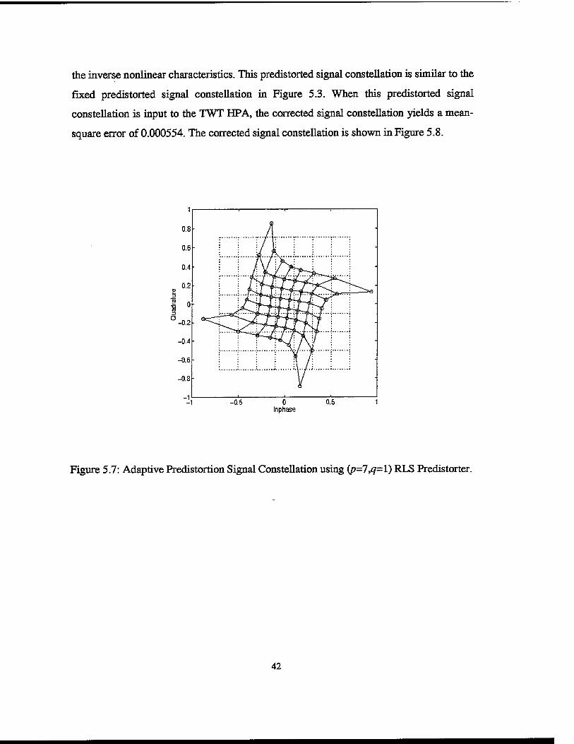
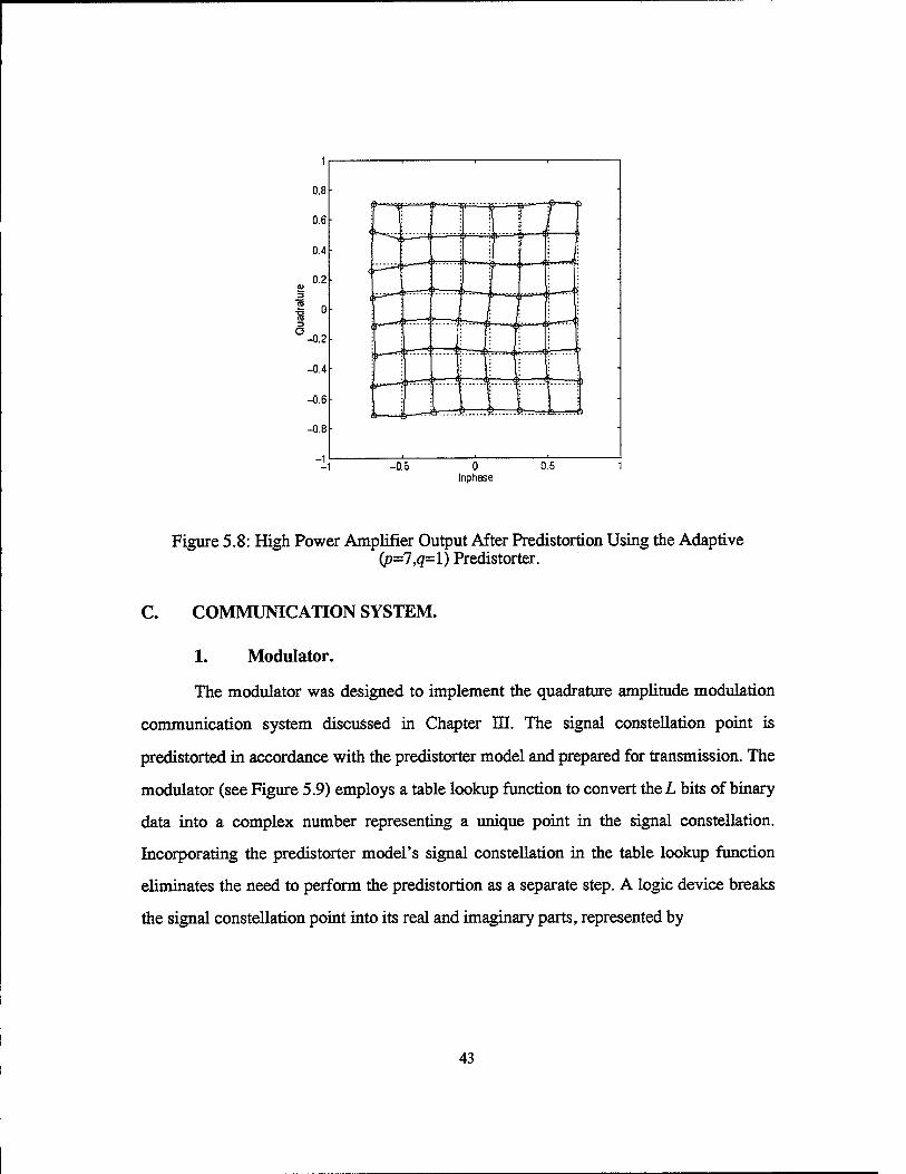
B. ADAPTIVE PREDISTORTER ................................. 41
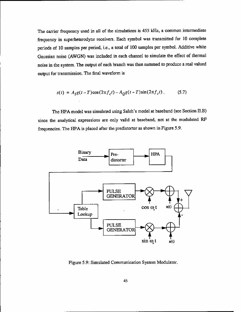
C. COMMUNICATION SYSTEM ................................. 43 1. Modulator ............................................. 43 2. Demodulator ........................................... 46 3. Signal-to-Noise Ratio .................................... 48
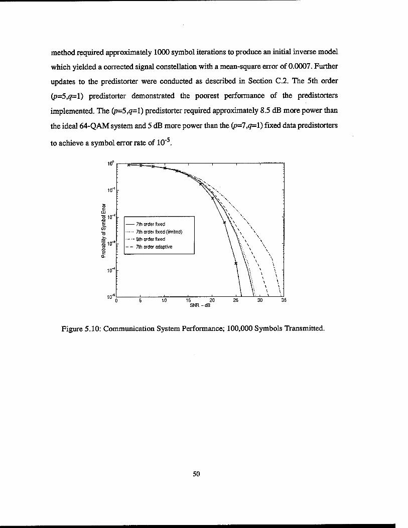
D. COMMUNICATION SYSTEM PERFORMANCE .................. 49
VI. CONCLUSIONS .................................................... 51
A. CONCLUSIONS ............................................. 51
B. FUTURE WORK ............................................ 52
APPENDIX A. MA TLAB COMPUTER CODE FOR DETERMINING THE NON-LINEAR DATA COEFFICIENTS ........................... 53
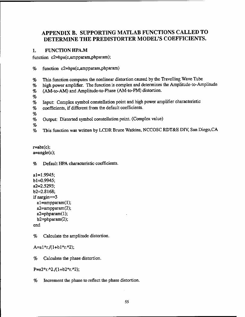
APPENDIX B. SUPPORTING MATLAB FUNCTIONS CALLED TO DETERMINE THE PREDISTORTER MODEL'S COEFFICIENTS ............ 55
APPENDIX C. MATLAB COMPUTER CODE CALCULATING THE FIXED PRE-DISTORTER MODEL .................................... 57
APPENDIX D. MA TLAB COMPUTER CODE FOR DETERIMINING THE PRE-FORMANCE OF A PREDISTORTER MODEL ................ 63
APPENDIX E. MA TLAB COMPUTER CODE FOR DETERMINING THE ADAPTIVE PREDISTORTER AND CO:MJviUNICATIONS SYSTEM PER-FORMANCE ........................................... 73
LIST OF REFERENCES ................................................. 85
INITIAL DISTRIBUTION LIST ........................................... 87
viii
L
I. INTRODUCTION
This thesis investigates two methods of analyzing the distortion characteristics of
High Power Amplifiers (HP A) found in modem digital communication systems. These
HP As can alter the transmitted signal to such an extent it is impossible to decode correctly.
The thesis focuses on using digital signal processing techniques to design a predistorter
which will result in the emitted signal being nearly intact and capable of proper decoding
by the receiver. The MATLAB programming language is used throughout this work to
determine the predistorter models and implement them in a 64 Quadrature Amplitude
Modulation (64-QAM) digital communication system.
The first predistortion technique investigated is a Volterra series approximation that
is based on a Minimum Mean Square Error (MMSE) approach to obtain a fixed predistorter
model. The second predistortion technique is a Recursive Least Squares (RLS) adaptive
algorithm. The first technique determines an inverse model predistorter which cannot be
altered once incorporated into the communication system. The second predistortion
technique, however, allows the predistorter to be updated periodically while the
communication system is operating.
The HP A serving as the base model for the transmitter is the Traveling Wave Tube
(TWT) high power amplifier. The TWT HP A was chosen since it is commonly employed
in a large variety of communication systems, and it has a commonly accepted model of its
nonlinear distortion characteristics in analytical form. The existence of this analytical
model precludes the need to experimentally measure the distortion characteristics of a
specillc high power amplifier since these characteristics may vary widely within the same
family ofHPAs.
This thesis focuses on the performance of the predistorter. A highly simplified
channel model is used in the simulation of the communication system for this purpose. The
MA TLAB implementation is designed with the assumption that perfect synchronization of
the phase and beginning of each symbol period is achieved. The results of the predistorter
1
models show how performance varies with the nonlinear order and memory of the Volterra
series approximation. The predistorter models are incorporated into a 64-QAM
communication system with an additive white gaussian noise (A WGN) channel. The
results of the communication system simulations indicate the ability of the predistorter to
correct the distortion by quantitatively measuring the probability of symbol error, P8, and
the effect of various signal-to-noise ratios on the probability of symbol error.
The thesis is organized as follows. Chapter IT discusses High Power Amplifiers.
Chapter ill covers digital communication techniques, specifically the 64-QAM system
used in simulations. Chapter IV details the theory of Volterra series, the recursive least
squares algorithm, and their application to predistorter modeling. Chapter V outlines the
simulation and results of the predistorter approximation. Chapter VI contains the
conclusions and areas for further study. The supporting computer code is contained in
Appendices A, B, C, D, and E.
2
II. HIGH POWER AMPLIFIERS
This chapter discusses the High Power Amplifier (HP A) and its characteristics. The
high power amplifier is used to produce signals with sufficient power to be detected and
correctly demodulated by the receiver. High power amplifiers are divided into classes
based upon the input and output voltage relationship. This influences the power efficiency
of the HP As and results in distortion of the output signal if the amplifier cannot transition
during its cycles properly. Specifically, power amplifiers with high power efficiencies can
significantly distort a signal during operation. The later sections of this chapter discuss the
distortion of these amplifiers.
A. CLASSES OF AMPLIFIERS.
Amplifiers are employed to scale the voltage and power levels in most electronics
systems. These amplifiers are designated by their class of operation. An amplifier's class
is judged by its input-output voltage relationship. Some of these classes and an explanation
of their input-output voltage relationships are summarized below.
1. Class A.
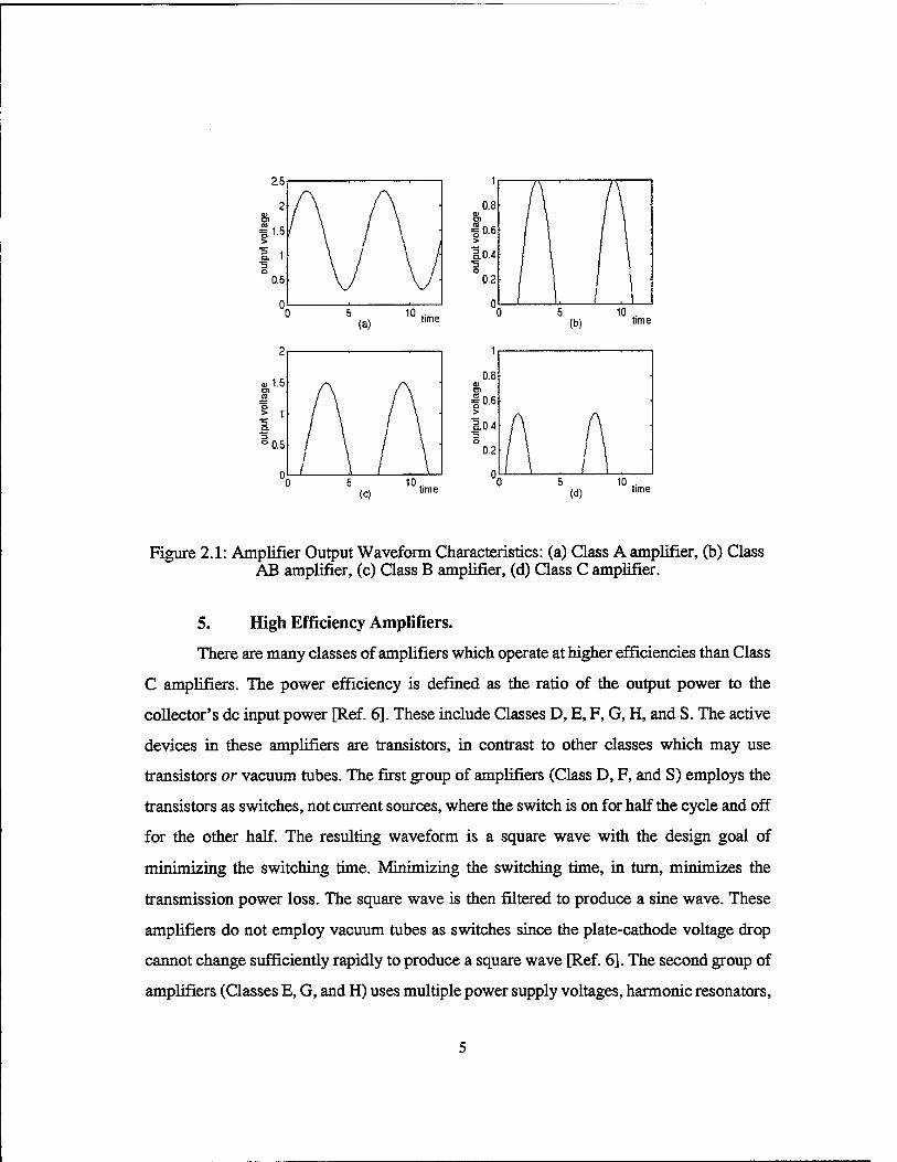
Class A amplifiers are designed to operate in a linear manner, similar to small signal
amplifiers. The distinctive waveform of a Class A amplifier shows the output current flows
for the entire cycle (Figure 2.1 (a)). Class A amplifiers are typically used as low level driver
amplifiers and in applications where other types of amplifiers cannot be used easily, such
as at microwave frequencies. The primary disadvantage of a Class A amplifier is its high
quiescent power loss, resulting in a maxim~ theoretical efficiency of only 50 percent
[Refs. 1 and 2].
2. Class B.
Class B amplifiers are biased so that conduction occurs only during one-half, or
180°, of a cycle of the input voltage (Figure 2.1 (b)). These amplifiers can be found in
medium and high power linear applications, such as in High Frequency Single Side Band
(HF SSB). Class B amplifiers commonly place a pair of active devices (transistors or
3
vacuum tubes) 180° out of phase with each other such that only one device is active at a
time during operation. The efficiency of a Class B amplifier is greater than Class A or AB,
a maximum theoretical efficiency of 78.5 percent, but its operation does generate some
nonlinear distortion [Refs. 1, 2, and 4].
3. Class AB.
Class AB operation is a compromise between Class A and Class B. Its current flows
for more than 180° and less than 360° (Figure 2.1 (c)). This compromise yields increased
efficiency over the Class A amplifier and less harmonic distortion than the Class B
amplifier [Ref. 3].
4. Class C.
Class C amplifiers have a higher bias than Class B, well beyond cutoff. This biasing
causes their conduction to occur for less than one-half, or less than 180°, of a duty cycle
(Figure 2.1 (d)). Typically, the conduction interval is in the range of 120°- 150° of biasing,
and the power efficiency is in the range of 60 - 80 percent with the active device in or near
the saturation region. This makes them ideal for RF transmission applications.
Class C amplifiers are found primarily at the transmitter end of long haul
communication systems where high output power levels are required, but proportionality
between the input and output voltages is not critical. For example, they are employed as
radio and television transmitters of 50 kW (or more) and LORAN Navigation Stations of 1
MW. Class C high power amplifiers may employ solid state or vacuum tube active devices.
Vacuum tubes are the workhorses of high power applications.
Class C amplifiers are able to achieve high efficiency if the duration of the current
flow is very small, such as when the voltage drop between the cathode and the plate is at
its lowest. Practical applications require a trade off between the amplifier's efficiency and
its power output since lower voltage drops reduce the input and output power. Transistors
employed as Class C amplifiers have similar operations but are limited in their power and
frequency ranges. Transistors are principally found in low power applications since care
must be taken not to exceed their current limit [Refs. 4 and 5].
4
:; 1 c. :; 0
0.5
0 0 5
(a)
2
., 1.5 "' .!!! g 1 a. :; 0 0.5
(c)
0.8 2l, ,g 0.6 > ].o.4 :; 0
0.2
0 10 time
0.8 ., "' ,g 0.6 > a.o.4 :; 0
0.2
0 5 (b)
10 . t1me
10 time
Figure 2.1: Amplifier Output Waveform Characteristics: (a) Class A amplifier, (b) Class AB amplifier, (c) Class B amplifier, (d) Class C amplifier.
5. High Efficiency Amplifiers.
There are many classes of amplifiers which operate at higher efficiencies than Class
C amplifiers. The power efficiency is defmed as the ratio of the output power to the
collector's de input power [Ref. 6]. These include Classes D, E, F, G, H, and S. The active
devices in these amplifiers are transistors, in contrast to other classes which may use
transistors or vacuum tubes. The first group of amplifiers (Class D, F, and S) employs the
transistors as switches, not current sources, where the switch is on for half the cycle and off
for the other half. The resulting waveform is a square wave with the design goal of
minimizing the switching time. Minimizing the switching time, in turn, minimizes the
transmission power loss. The square wave is then filtered to produce a sine wave. These
amplifiers do not employ vacuum tubes as switches since the plate-cathode voltage drop
cannot change sufficiently rapidly to produce a square wave [Ref. 6]. The second group of
amplifiers (Classes E, G, and H) uses multiple power supply voltages, harmonic resonators,
5
and other circuit technologies. The overall advantage of high efficiency amplifiers is the
ability to use smaller power supplies to generate the same output as other classes of
amplifiers. These amplifiers can be found in cellular phone systems and other applications
where limited power is available [Ref. 6].
B. INTERMODULA TION DISTORTION.
Intermodulation Distortion (IMD) is the nonlinear distortion produced as a result of
the inability of an RF power amplifier to exactly reproduce the envelope and phase of an
amplified signal. This distortion has many sources. They include: crossover effects, gain
reduction at high current, variation of collector capacitance with collector voltage, and
device saturation. This thesis considers the nonlinear distortion resulting from an HP A
operating at its saturation point [Ref. 4].
The nonlinear distortion of an HP A operating at its saturation point has two
components: Amplitude-to-Amplitude (AM-to-AM) conversion and Amplitude-to-Phase
(AM-to-PM) conversion. AM-to-AM conversion is a result of the amplifier's inability to
output an exact replica of the input waveform [Refs. 2 and 6]. AM-to-PM conversion
results from the signal being passed through a reactance larger than the collector's load
resistance causing a phase variation in the carrier frequency. AM-to-PM conversion is not
detectable by an envelope detector but does cause unwanted sideband frequencies. The
extent of this nonlinear distortion varies with the class, age, temperature, and composition
of the HPA. As a result, many HP As must be measured experimentally to obtain an
accurate model of their nonlinear distortion characteristics. One significant exception to the
need to model nonlinear distortion experimentally is the Traveling Wave Tube (TWT)
HPA. An analytical model, developed by Saleh [Ref. 7], serves as a standard model for
research into the design of predistorters and channel effects on signals amplified using a
TWT. The AM-to-AM conversion is characterized by:
(2.1)
6
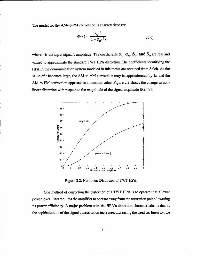
The model for the AM-to-PM conversion is characterized by:
(2.2)
where r is the input signal's amplitude. The coefficients aa, a+, ~a• and~+ are real and
valued to approximate the standard TWT HPA distortion. The coefficients identifying the
HPA in the communication system modeled in this thesis are obtained from Saleh. As the
value ofr becomes large, the AM-to-AM conversion may be approximated by 1/r and the
AM-to-PM conversion approaches a constant value. Figure 2.2 shows the change in non
linear distortion with respect to the magnitude of the signal amplitude [Ref. 7].
% "Transmit" the predistorter model through the high power amplifier.
yv = hpa(distdata); % Reshape the vectors into 8 x 8 matrices for plotting.
57
yyv=reshape(yv,8,8); dd=reshape(distdata,8,8);
% Calculate the mean square error of the resulting signal constellation emitted from the
% high power amplifier.
se = sum(sum(abs(yyv-conj(xi)).A2));sx=size(xi); msefinal=se/(sx(l)*sx(2));
% Plot the results.
figure(l), orient tall
% Plot the predistorter model.
subplot(211) plot(distdata,'o'), hold on,plot(xi,':'),plot(rot90(xi),':'),plot(dd,'-'), plot(rot90(dd),'-'),aspectl title(['Nonlinearity order= ',num2str(ord-l),', Data points= ',num2str(points)])
% Plot the emitted signal constellation output by the high power amplifier.
subplot(212) plot(yyv,' o'), hold on, plot( xi,': '),plot(rot90(xi), ': '),plot(yyv, '-') plot(rot90(yyv),'-'),aspectl title(['F7 .m, HPA Output, MSE = ',num2str(msefinal)])
2. FUNCTION FIX7 .M.
function [distdata,yyv,gl,g3,g5,g7,il,i3,i5,i7] = fix7(ord,x,points)
% function [distdata,yyv,gl,g3,g5,g7,il,i3,i5,i?] = fix7(ord,x,points)
% % This function calculates the inverse of the nonlinear distortion caused by high power % amplifiers using a fixed Volterra Series approximation. The inverse model calculated % is used to create a predistorter to correct the amplifier's distortion. This function is % called by the script file f7 .m. It in turn calls the function order7 .m to determine the % nonlinear data terms used to build the data matrix used in the solution of the Volterra % kernel coefficients. The Volterra kernel coefficients are solved using a Least Squares % technique. % % Input: The memory of the system (ord), the signal constellation in vector form (x), and % the number of data points to be used in the Least Squares solution .. % % Output: The predistorter model in vector form (distdata), the Volterra kernel coefficients
58
% (g1, g3, g5, and g7), and the counters for the number of nonlinearity terms % (il, i3, i5, and i7). %
% Generate the random vector of data points to be used in the Least Squares solution.
ra=rand(1,points);d=zeros(1,points);
% Establish a table and assign the random number vector's elements to a point in the % signal constellation.
TAB = [linspace(0,1,64)' (1:64)']; zz = fix(table1(TAB,ra)); d =x(zz);
% Initialize a shift register with the number of states equal to ord.
sr = d(1:ord)
% Simulate the distortion using Saleh's equations of the data and the signal constellation.
ysaleh = hpa(conj(x')); ysalehd = hpa(conj(d'));
% Create counters for the length of the data and the signal constellation.
[m n] = size(ysalehd) [nx mx] = size(x);
% Build the nonlinear data matrix, X, by shifting in the data. One column for each data point.
fork= 1:m
sr = [ysalehd(k) sr(1,1:ord-1)];
% Call the function order? .m to build a row of the data matrix.
% Simulate the predistortion using the Volterra Series. % Reinitialize the shift register to input the QAM signal constellation.
r = zeros(1~ord); yv = zeros(1,m);
% Iteratively shift in each point of the signal constellation.
fork= 1:64 r = [x(k) r(1~1:ord-1)];
% Create the nonlinearity data matrix vector, called rworking in this call.
[ rworking,il~i3~i5,i7] = order7(r,ord);
% Establish counters for each nonlinearity order.
y1 = O;y3 = O;y5 = O;y7 = 0;
% Calculate the first order terms.
r1 = rworking(1:ord); y1 = r1'*g1;
% Calculate the third order terms.
r3 = rworking(il+l:i3); y3 =r3' * g3;
% Calculate the fifth order terms.
60
r5 = rworking(i3+ 1 :i5); y5 =r5' * g5;
% Calculate the seventh order terms.
r7 = rworking(i5+ 1 :i7); y7 =r7' * g7;
% Calculate the distorter data term for the signal constellation using the first through seventh % order nonlinearity terms. This is for only one signal constellation point. One iteration % must be performed for each point in the signal constellation.
distdata(1,k) = y1 + y3 + y5 + y7;
end
61
62
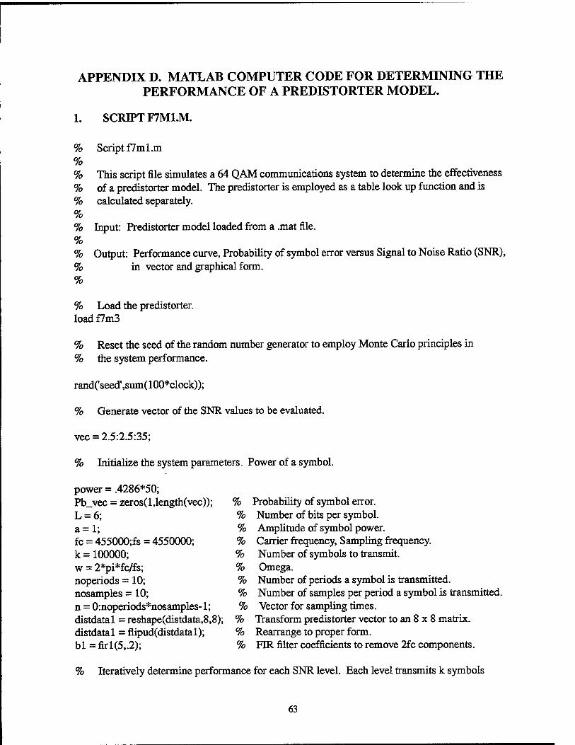
APPENDIX D. MATLAB COMPUTER CODE FOR DETERMINING THE PERFORMANCE OF A PREDISTORTER MODEL.
1. SCRIPT F7Ml.M.
% Script f7ml.m % % This script file simulates a 64 QAM communications system to determine the effectiveness
% of a predistorter model. The predistorter is employed as a table look up function and is
% calculated separately. % % Input: Predistorter model loaded from a .mat file. % % Output: Performance curve, Probability of symbol error versus Signal to Noise Ratio (SNR),
% in vector and graphical form. %
% Load the predistorter. loadf7m3
% Reset the seed of the random number generator to employ Monte Carlo principles in
% the system performance.
rand('seed',sum(100*clock));
% Generate vector of the SNR values to be evaluated.
vee= 2.5:2.5:35;
% Initialize the system parameters. Power of a symbol.
power = .4286*50; Pb_vec = zeros(1,length(vec)); L=6; a= 1; fc = 455000;fs = 4550000; k= 100000; w = 2*pi*fc/fs; noperiods = 10; nosamples = 10; n = O:noperiods*nosamples-1; distdata1 = reshape(distdata,8,8); distdata1 = fiipud(distdata1); b1 = fir1(5,.2);
% Probability of symbol error. % Number of bits per symbol. % Amplitude of symbol power. % Carrier frequency, Sampling frequency. % Number of symbols to transmit. % Omega. % Number of periods a symbol is transmitted. % Number of samples per period a symbol is transmitted. % Vector for sampling times.
% Transform predistorter vector to an 8 x 8 matrix. % Rearrange to proper form. % FIR filter coefficients to remove 2fc components.
% Iteratively determine performance for each SNR level. Each level transmits k symbols
63
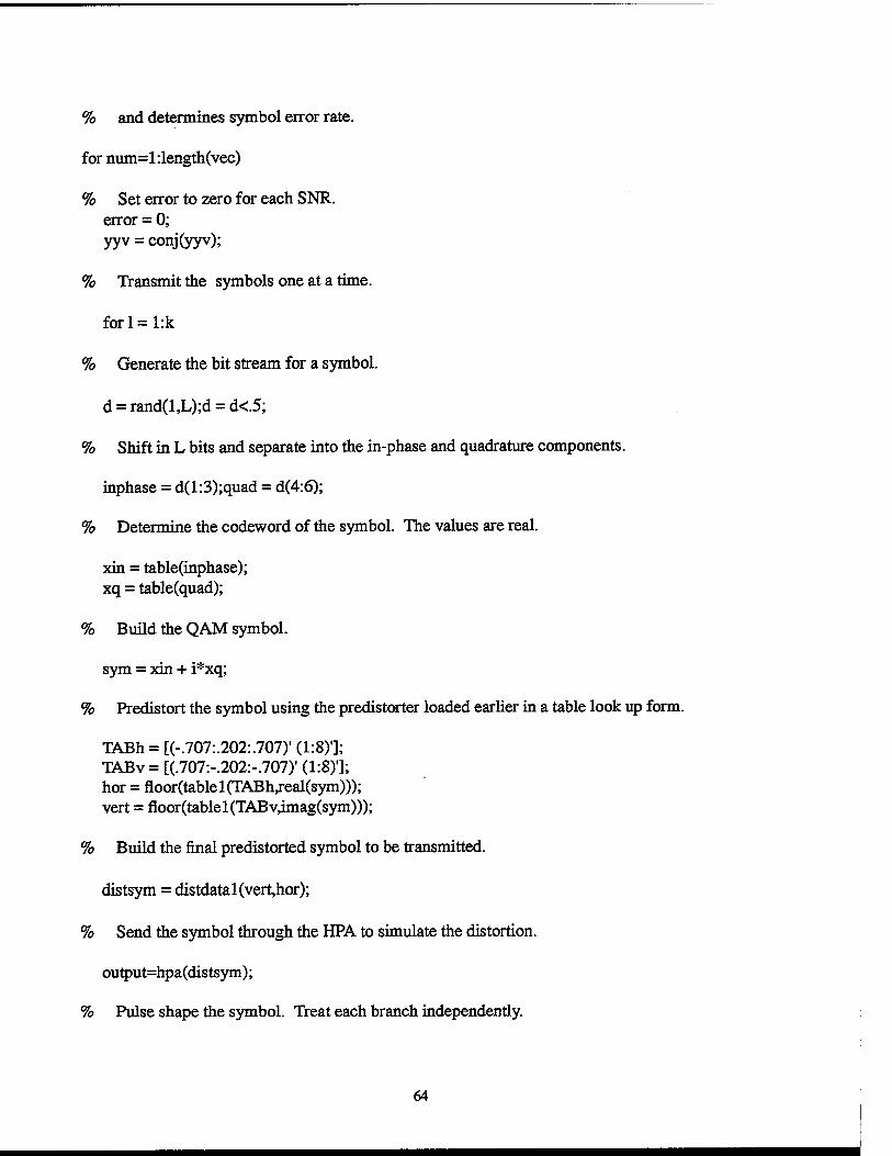
% and determines symbol error rate.
for num=1:length(vec)
% Set error to zero for each SNR. error= 0; yyv = conj(yyv);
% Transmit the symbols one at a time.
for 1 = 1:k
% Generate the bit stream for a symbol.
d = rand(1,L);d = d<.5;
% Shift in L bits and separate into the in-phase and quadrature components.
inphase = d(1:3);quad = d(4:6);
% Determine the codeword of the symbol. The values are real.
xin = table(inphase); xq =table( quad);
% Build the QAM symbol.
sym = xin + i*xq;
% Predistort the symbol using the predistorter loaded earlier in a table look up form.
% Build the received signal into the received symbol for detection.
y = ycth- ysth*i; %Negative to account for the change in threshold level.
% Estimate the symbol transmitted using a "choose the largest strategy".
sest = mqam_det(y,L,a);
65
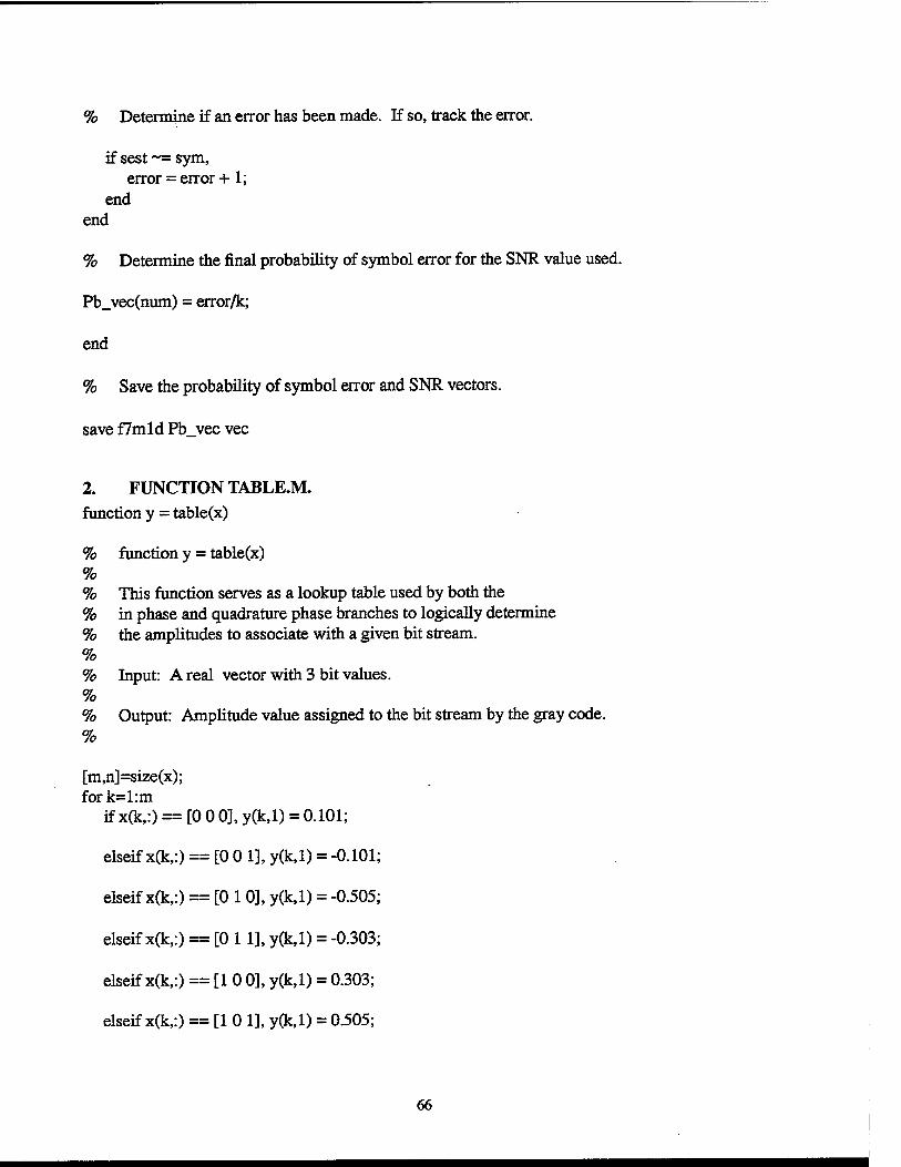
% Determine if an error has been made. If so, track the error.
if sest -= sym, error= error+ 1;
end end
% Determine the final probability of symbol error for the SNR value used.
Pb_vec(num) = error/k;
end
% Save the probability of symbol error and SNR vectors.
save f7m1d Pb_ vee vee
2. FUNCTION TABLE.M. function y = table(x)
% function y = table(x) % % This function serves as a lookup table used by both the % in phase and quadrature phase branches to logically determine % the amplitudes to associate with a given bit stream. % % Input: A real vector with 3 bit values. % % Output: Amplitude value assigned to the bit stream by the gray code. %
[m,n]=size(x); fork=1:m
if x(k,:) == [0 0 0], y(k,1) = 0.101;
elseifx(k,:) == [0 0 1], y(k,1) = -0.101;
elseifx(k,:) == [0 1 0], y(k,1) = -0.505;
elseifx(k,:) == [0 11], y(k,1) = -0.303;
elseifx(k,:) == [1 0 0], y(k,1) = 0.303;
elseif x(k,:) == [1 0 1], y(k, 1) = 0.505;
66
elseifx(k,:) == [11 0], y(k,1) = -0.707;
elseif x(k,:) == [1 11], y(k,l) = 0.707;
end end
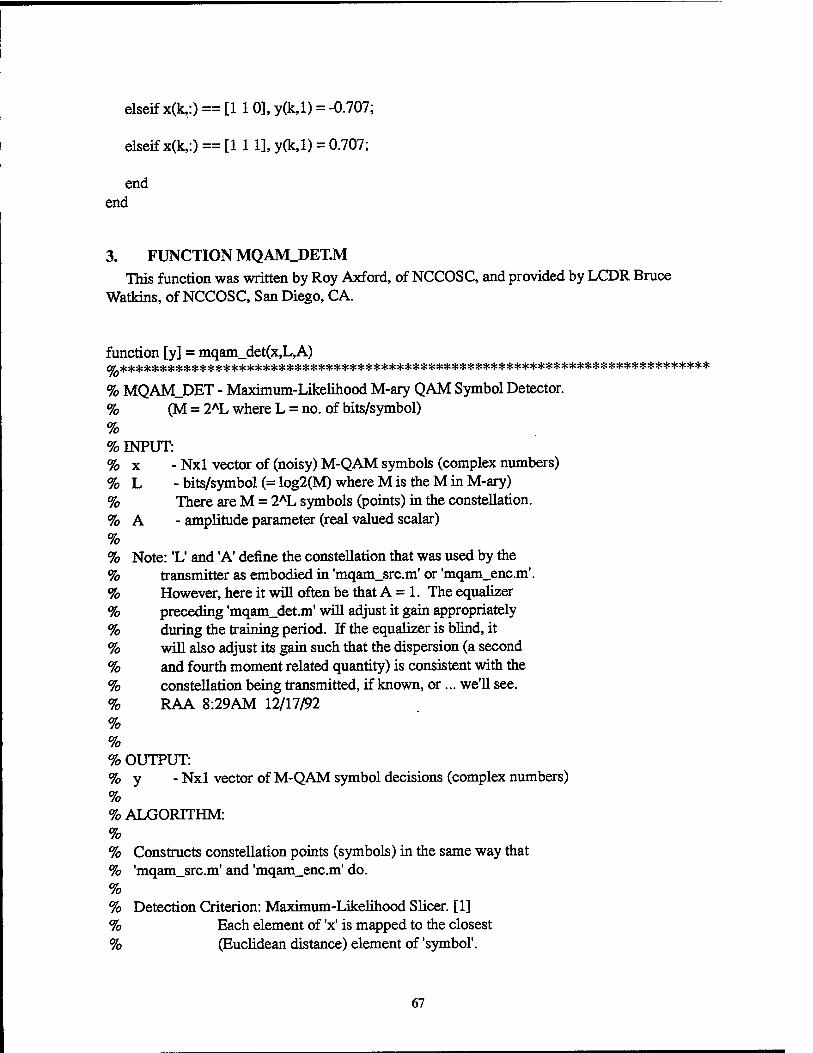
3. FUNCTION MQAM_DET.M
This function was written by Roy Axford, of NCCOSC, and provided by LCDR Bruce
~ MQAM_DET- Maximum-Likelihood M-ary QAM Symbol Detector.
~ (M = 2"L where L = no. of bits/symbol) ~
~INPUT: ~ x - Nx1 vector of (noisy) M-QAM symbols (complex numbers)
~ L - bits/symbol (= log2(M) where M is theM in M-ary)
~ There are M = 2"L symbols (points) in the constellation.
~ A -amplitude parameter (real valued scalar)
~ ~ Note: 'L' and 'A' define the constellation that was used by the % transmitter as embodied in 'mqam_src.m' or 'mqam_enc.m'.
% However, here it will often be that A = 1. The equalizer % preceding 'mqam_det.m' will adjust it gain appropriately
~ during the training period. If the equalizer is blind, it
% will also adjust its gain such that the dispersion (a second
~ and fourth moment related quantity) is consistent with the
~ constellation being transmitted, if known, or ... we'll see.
~ RAA 8:29AM 12/17/92 ~
~ ~OUTPUT:
% y - Nxl vector ofM-QAM symbol decisions (complex numbers)
% % ALGORITHM: ~ ~ Constructs constellation points (symbols) in the same way that % 'mqam_src.m' and 'mqam_enc.m' do. % ~ Detection Criterion: Maximum-Likelihood Slicer. [1]
~ Each element of 'x' is mapped to the closest
~ (Euclidean distance) element of 'symbol'.
67
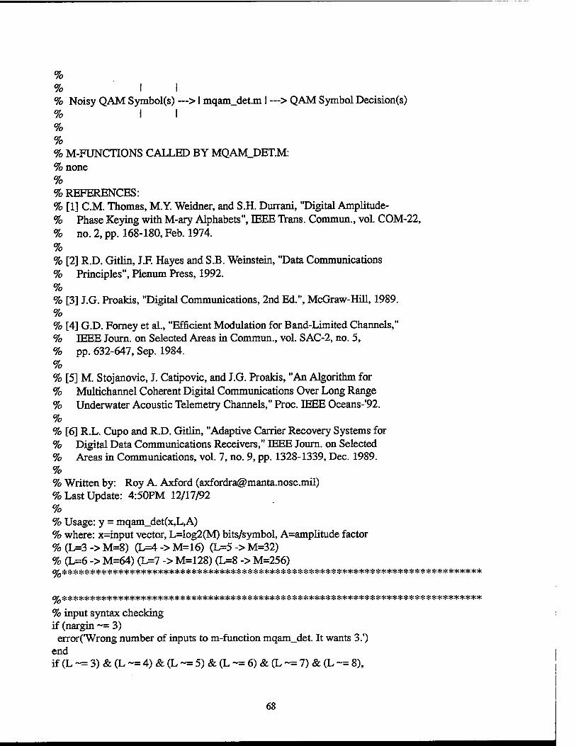
% % % Noisy QAM Symbol(s) ---> I mqam_det.m I ---> QAM Symbol Decision(s) % I I % % % M-FUNCTIONS CALLED BY MQAM_DET.M: %none % %REFERENCES: % [1] C.M. Thomas, M.Y. Weidner, and S.H. Durrani, "Digital Amplitude-
% % [2] R.D. Gitlin, J.F. Hayes and S.B. Weinstein, "Data Communications % Principles", Plenum Press, 1992. % % [3] J.G. Proakis, "Digital Communications, 2nd Ed.", McGraw-Hill, 1989. % % [ 4] G.D. Forney et al., "Efficient Modulation for Band-Limited Channels," % IEEE Journ. on Selected Areas in Commun., vol. SAC-2, no. 5, % pp. 632-647, Sep. 1984. % % [5] M. Stojanovic, J. Catipovic, and J.G. Proakis, "An Algorithm for
% Multichannel Coherent Digital Communications Over Long Range
% Underwater Acoustic Telemetry Channels," Proc. IEEE Oceans-'92. % % [6] R.L. Cupo and R.D. Gitlin, "Adaptive Carrier Recovery Systems for % Digital Data Communications Receivers," IEEE Journ. on Selected % Areas in Communications, vol. 7, no. 9, pp. 1328-1339, Dec. 1989. % %Written by: Roy A. Axford ([email protected]) % Last Update: 4:50PM 12/17/92 % % Usage: y = mqam_det(x,L,A) % where: x=input vector, L=log2(M) bits/symbol, A=amplitude factor % (L=3 -> M=8) (L=4 -> M=16) (L=5 -> M=32) % (L=6 -> M=64) (L=7 -> M=128) (L=8 -> M=256) %***************************************************************************
%*************************************************************************** % input syntax checking if (nargin -= 3)
error('Wrong number of inputs tom-function mqam_det. It wants 3.') end if (L -= 3) & (L -= 4) & (L -= 5) & (L -= 6) & (L -= 7) & (L -= 8),
68
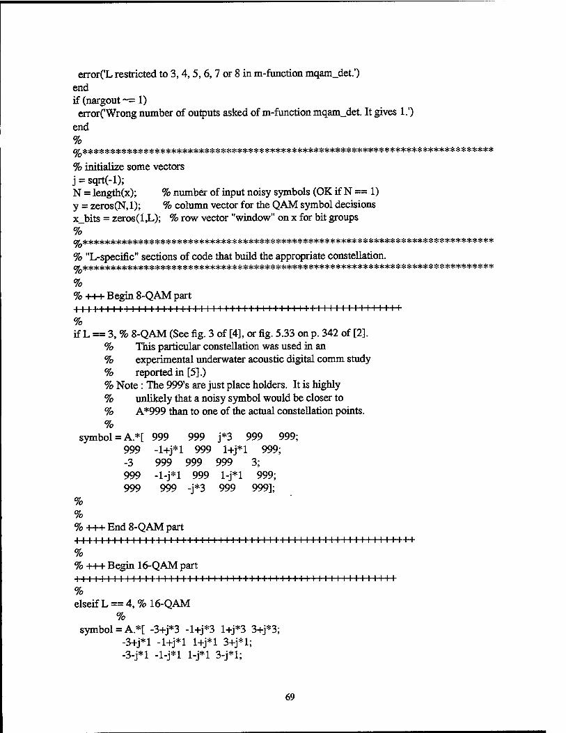
error('L restricted to 3, 4, 5, 6, 7 or 8 in m-function mqam_det.') end if (nargout -= 1) error('Wrong number of outputs asked of m-function mqam_det. It gives 1.')
end % %*************************************************************************** % initialize some vectors j = sqrt( -1); N = length(x); % number of input noisy symbols (OK if N == 1) y = zeros(N,1); % column vector for the QAM symbol decisions x_bits = zeros(1,L); %row vector "window" on x for bit groups % %*************************************************************************** % "L-specific" sections of code that build the appropriate constellation. %*************************************************************************** % % +++Begin 8-QAM part +++11111111111111111111111111111111111111111111111111
% if L == 3,% 8-QAM (See fig. 3 of [4], or fig. 5.33 on p. 342 of [2].
% This particular constellation was used in an % experimental underwater acoustic digital comm study % reported in [5].) % Note : The 999's are just place holders. It is highly % unlikely that a noisy symbol would be closer to % A *999 than to one of the actual constellation points. %
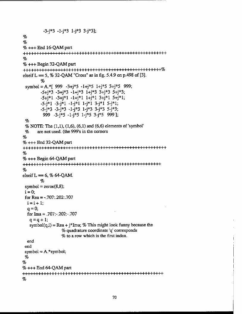
% %NOTE: The (1,1), (1,6), (6,1) and (6,6) elements of 'symbol' % are not used. (the 999's in the comers
% % +++End 32-QAM part +++11111111111111111111111111111111111111111111111111+
% % +++Begin 64-QAM part 111111111111111111111111111111111111111111111111++++
% elseifL == 6,% 64-QAM.
% symbol = zeros(8,8); i=O; for Rea= -.707:.202:.707 i = i + 1; q =0; for Ima = .707:-.202:-.707 q =q + 1; symbol(q,i) = Rea+ j*Ima; % This might look funny because the
% quadrature coordinate 'q' corresponds % to a row which is the first index.
end end symbol = A. *symbol; %
% % +++End 64-QAM part +++11111111111111111111111111111111111111111111111111
%
70
% +++Begin 128-QAM part +++11111111111111111111111111111111111111111111111 % elseifL = 7,% 128-QAM. (See fig. 5.4.9 on p.498 of [3].) % % % % %
Also, a perhaps more practical128-QAM constellation is shown on p. 1337 of [6] with varying degrees of distortion caused by phase jitter. RAA
% Create the 128-QAM constellation symbols. % Some of the symbols won't be used (i.e. the "comers" of the cross). %These square shaped regions are (q,i) = (1:2, 1:2), % (11:12, 1:2), % (1:2, 11: 12), % (11:12, 11:12).
% symbol= zeros(12,12); i = 0; for Rea = -11 :2: 11 i = i + 1; q =0; for Ima = 11:-2:-11
q =q + 1; symbol(q,i) =Rea+ j*Ima; % This might look funny because the
%quadrature coordinate 'q' corresponds % to a row which is the first index.
% If we're in one of those comer areas, we need place holders: if ((q==1)&(i=1))1((q==1)&(i==2))1((q==2)&(i==1))1((q==2)&(i==2))
% % +++End 128-QAM part +++Ill I I II Ill I I II I I II II I II I I I II II I II II IIIII IIIII++++ % % +++ Begin 256-QAM part 111111111111111111111111111111111111111111111111++ %
71
elseif L = 8, % 256-QAM. %
symbol= zeros(16,16); i=O; for Rea= -15:2:15 i = i + 1; q =0; for Ima = 15:-2:-15 q = q + 1; symbol(q,i) =Rea+ j*lrna; % This might look funny because the
%quadrature coordinate 'q' corresponds % to a row which is the first index.
end end % symbol =A. *symbol;
% +++End 256-QAM part I I I I I I I I I I I I I I I I I I I I I I I I I I I I I I I I I I I I I I I I I I I I I I I I I I I I I
% end %This 'end' is for the ifs and elseifs above regarding the value
% of L, the number of bits per symbol. % % So, at this point we've constructed the appropriate constellation. %Now, for each x(n) we calculate the Euclidean distance between x(n) and % each symbol in the constellation. We decide for the symbol that is % closest to x(n) and assign this symbol to y(n). %(Ref.: MATLAB Manual, Reference Section "max, min".) % forn= 1:N
% quadrature coord. is row index % in-phase coord. is column index y(n) = symbol(q_coord_of_closest, i_coord_of_closest);
end % % /* --------------end of m-function mqam_det.m ----------------------------*/
72
APPENDIX E. MATLAB CODE FOR DETERMINING THE ADAPTIVE PREDISTORTER AND COMMUNICATIONS SYSTEM PERFORMANCE.
1. SCRIPT FILE A7.M.
% Script file a7.m % % This script file calculates the inverse model of the high power amplifier's distortion % characteristics using the Recursive Least Squares algorithm. The coefficients are % based upon the Volterra kernel coefficients seen in other code used in this thesis. % This script file's functions use the same function order7.m to determine the nonlinear % data coefficients used in the RLS algorithm. The functions called by this script include
% ad7 .m, berold.m, and ad7mod.m. These functions are used to determine the initial pre
% distorter model, determine the communications system performance, and update the
% predistorter at a specified interval. % % Input: The signal constellations for QAM are loaded form a .mat file. % % Output: The predistorter model and communication system performance.
%
% Reset the seed of the random number generator to employ Monte Carlo theory.
rand('seed',sum(lOO*clock));
% Identify the memory of the system, ord - 1.
ord= 2;
% Load the QAM signal constellations.
loadqam
% Identify the signal constellation to be employed and transformed into vector form.
xi= c64; x=reshape(xi, 1,64 );
% Identify the number of iterations to be used in generating the predistorter.
points = 1000;
% Generate a random vector to assign symbols from the signal constellation.
% Simulate the distortion using the Volterra Series. % Reinitialize the shift register to input the QAM signal constellation.
r = zeros(1,ord);
% Iteratively shift in each point of the signal constellation.
fork= 1:64
r = [x(k) r(1,1:ord-1)];
77
% Create the nonlinearity data vector, called rworking in this call.
[rworking,il,i3,i5,i7] = order7(r,ord);
% Initialize values for each nonlinearity order.
yl = O;y3 = O;y5 = O;y7 = 0;
% Calculate the first order terms.
rl = rworking(l:ord); yl = rl'*gl;
% Calculate the third order terms.
r3 = rworking(il+l:i3); y3 =r3' * g3;
% Calculate the fifth order terms.
r5 = rworking(i3+1:i5); y5 =r5' * g5;
% Calculate the seventh order terms.
r7 = rworking(i5+ 1 :i7); y7 =r7' * g7;
% Calculate the predistorter data term for the signal constellation using the first through % seventh order nonlinearity terms. This is for only one signal constellation point. One % iteration must be performed for each point in the signal constellation.
distdata(l,k) = yl + y3 + y5 + y7;
end
3. FUNCTION BEROLD.M. function [buffer,Pbsub] = berold(dd,vec)
% function [buffer,Pbsub] = berold (dd,vec) % % This function simulates the 64 QAM communications system to determine the effectiveness % of the predistorter for each iteration of the update. The predistorter is employed as a % table look up function and is calculated with the functions ad7.m and ad7mod.m. %
78
% Input: Predistorter model (dd),a dn Signal-to-Noise ratio range (vee).
% % Output Last data symbols transmitted to be used in the RLS update, the length of the vector % is specified internally. (buffer) The probability symbol error for the current
% Power of the symbol. % Probability of symbol error vector.
% number of bits/symbol. % amplitude of the signal. % carrier frequency, sampling frequency. % number of symbols to transmit. % Omega.
% number of periods per symbol. % number of samples per period. % vector for samplig times. % Rearrange for proper form. % Output vector with last symbols transmitted. % FIR filter coefficients to remove 2fc components.
% Iteratively determine the performance for each SNR level. Each level transmits k symbols
% determines the symbol error rate.
for num=l:length(vec)
% Set the error to zero.
error= 0; yyv = conj(yyv);
% Transmit the symbols one at a time.
for 1 = 1:k
% Generate the bit stream for the symbol.
d = rand(l,L);d = d<.5;
% Shift in L bits and separate into the in-phase and quadrature components.
inphase = d(1:3);quad = d(4:6);
% Determine the codeword of the symbol. The values are real..
79
xin = table(inphase); xq = table(quad);
% Build the QAM symbol.
sym = xin + i*xq;
% Predistort the symbol using the predistorter loaded earlier in a table look up form.
% Build the received signal into the received symbol for detection.
y = ycth + ysth*i;
% Estimate the symbol transmitted using a "choose largest strategy" and determine if in
% error.
sest = mqam_det(y,L,a); if sest -= sym,
error = error + 1; end
% Determine if the symbol must be buffered.
ifl > k-lOOO,buffer(l,l-k+lOOO) = sym;end end
% Determine the probability of error for this iteration.
Pbsub(num) = error/k;
end
4. FUNCTION AD7MOD.M.
function [distdata,P,gl,g3,g5,g7,il,i3,i5,i7] = ad7mod(ord,x,buffer,points,P)
% function [distdata,P,gl,g3,g5,g7 ,il,i3,i5,i7] = ad7mod(ord,x,buffer,points,P)
% % This funciton calculates the inverse of the nonlinear distortion caused by the high power
% amplifier using the Recursive Least Squares algorithm. This function is similar to the
81
% function ad7 .m but has been modified. The modifications include passing the buffer and % previous inverse correlation matrix, P. This function is called by the script file a7 .m and % calculates the inverse distortion model. % % Input: The memory of the system (ord), the signal constellation in vector form (x), the % buffer from the immediately preceding communications system simulation (buffer), % the number of recursive steps to obtain the predistorter constellation (points), and % the previous inverse correlation matrix (P). % % Output: The predistorter in vector form (distdata), the inverse correlation matrix (P), the % Volterra kemal coefficients (gl,g3,g5,g7), and the counters for the number of % nonlinearity terms (il,i3,i5,i7).
% Initialize a shift register with the number of states equal to ord.
sr = zeros(l,ord);
% Simulate the distortion, using Saleh's equations, of the data and signal constellations.
% Simulate the Distortion using the Volterra Series. % Reinitialize the shift register to input the QAM signal constellation.
r = zeros(1,ord);
% Iteratively shift in each point of the signal constellation.
fork= 1:64
r = [x(k) r(1,1:ord-1)];
% Create the nonlinearity data vector, called rworking in this call.
[rworking,i1,i3,i5,i7] = order7(r,ord);
% Initialize values for each nonlinearity value.
y1 = O;y3 = O;y5 = O;y7 = 0;
% Calculate the first order terms.
r1 = rworking(1:ord); y1 = r1'*g1;
% Calculate the third order terms.
r3 = rworking(i1+1:i3); y3 = r3' * g3;
% Calculate the fifth order terms.
83
r5 = rworking(i3+ 1 :i5); y5 =r5' * g5;
% Calculate the seventh order terms.
r7 = rworking(i5+1:i7); y7 =r7' * g7;
% Calculate the predistorter data term for the signal constellation using the first through % seventh order nonlinearity terms. This is for only one signal constellation point. One % iteration must be performed for each point in the signal constellation.
distdata(l,k) = yl + y3 + y5 + y7;
end
84
LIST OF REFERENCES
1. Morris, N. H., Industrial Electronics for Technicians and Technician Engineers, New York: McGraw-Hill, 1970.
2. Terman, Frederick Emmons, et. al., Electronic and Radio Engineering, New York: McGraw-Hill, 1955.
4. Sedra, Adel and Smith, Kenneth, Microelectronics Circuits, Fort Worth, TX: Saunders College Publishing, 1991.
5. Gottlieb, Irving M., Practical RF Power Design Techniques, New York: TAB Books, 1993.
6. Krauss, Herbert L., et. al., Solid State Radio Engineering, New York: John Wiley & Sons, 1980.
7. A. A. M. Saleh, "Frequency-Independent and Frequency-Dependent Nonlinear Models of TWT Amplifiers," IEEE Trans. on Communications, Vol. COM-29, pp. 1715- 1720, Nov. 1980.
8. E. Biglieri, et. al., "Analysis and Compensation of Nonlinearities in Digital Transmission Systems," IEEE Journal on Selected Areas in Communications, Vol. 6, pp. 42-51, Jan 1988.
9. S. Benedetto, et. al., "Modeling and Performance Evaluation of Nonlinear Satellite Links: A Volterra Series Approach," IEEE Transactions on Aerospace and Electronic Systems, Vol. AAES-15, pp. 494-506, July 1979.
10. Hoile, G., et. al., "Nonlinear MESFET Model for the Design of RF Power Amplifiers," lEE Proceedings-G. Vol. 139, No.5, pp. 574-580, Oct. 1992.
11. Hayashi, H., et. al., "Quasilinear Amplification using Self Phase Distortion Compensation Technique," IEEE Transactions on Microwave Theory and Technology, Vol. MTT-43, No. 11, pp. 2551-2564, Nov. 1995.
12. Fihel, A. and Sari, H., "Performance of Reduced-Bandwidth 16 QAM with Decision-Feedback Equalization," IEEE Trans. on Communications, Vol. COM-35, pp. 715-723, July 1987.
13. Cavers, J., "Amplifier Linearization Using a Digital Predistorter with Fast Adaptation and Low Memory Requirements," IEEE Trans. on Vehicular Technology, Vol. 39, No.4, pp. 374-882, Nov. 1990.
85
14. Watkins, B., et. al., "Neural Network based Adaptive Predistortion for the
Linearization of Nonlinear RF Amplifiers," Proceedings of MILCOM95,
Nov. 1995.
15. Watkins, B. et. al., "Model Based Neural Network Predistortion of Nonlinear Amplifiers," Proc. of International Conference on Neural Networks, Nov.
1996.
16. Stapleton, S., et. al., "Simulation and Analysis of an Adaptive Predistorter Utilizing a Complex Spectral Convolution," IEEE Trans. on Vehicular
Technology, Vol. 41, No. 4, pp. 387-394, Nov. 1992
17. Sklar, Bernard, Digital Communications: Fundamentals and Applications,
Englewood Cliffs, NJ: Prentice-Hall, 1988.
18. Frerking, Marvin E., Digital Signal Processing in Communications Systems,
New York: Van Nostrand Reinhold, 1994.
19. Proakis, John G., Digital Communications, New York: McGraw-Hill, 1995.
20. Lazzarin, G., et. al., "Nonlinearity Compensation in Digital Radio Systems," IEEE Trans: on Communications, Vol. 42, pp. 988-999, Apri11994.
21. Schetzen, Martin, "Nonlinear System Modeling Based on the Wiener Theory," Proceedings of the IEEE, Vol. 69, No. 12, Dec 1981.
22. Schetzen, Martin, The Volterra and Wiener Theories of Nonlinear Systems,
24. Rugh, Wilson, Nonlinear System Theory - The Volterra/Wiener Approach,
Baltimore: Johns Hopkins University Press, 1981.
25. Faulkner, M. and Mattsson, T., "Spectral Sensitivity of Power Amplifiers to Quadrature Modulator Misalignment," IEEE Trans. on Vehicular Technology,
Vol. 41, pp. 516-525, Nov. 1992.
26. Serfaty, S. et. al., "Cancellation of Nonlinearities in Bandpass QAM
1. Defense Technical Information Center..................................................................... 2 8725 John J. Kingman Rd., STE 0944 Ft. Belvoir, VA 22060-6218
2. Dudley Knox Library ................................................................................................. 2 Naval Postgraduate School 411 Dyer Rd. Monterey, CA 93943-5101
3. Chairman, Code EC ................................................................................................... 1 Department of Electrical and Computer Engineering Naval Postgraduate School Monterey, CA 93943-5121
4. Prof. Murali Tummala, Code EC{fu .......................................................................... 4 Department of Electrical and Computer Engineering Naval Postgraduate School Monterey, CA 93943-5121
5. Prof. Charles Therrien, Code EC/fi.. .. .. . . . . .. .... .. . . .... . . .. .. .. .. .. .. .. .. . . .. .. .. .. .. .. .. .. .. .. .. .. . . .. .. 1 Department of Electrical and Computer Engineering Naval Postgraduate School Monterey, CA 93943-5121
6. Richard North ............................................................................................................. 1 NCCOSC RDT&E DIV 53560 Hull St. San Diego, CA 92152-5001
7. LT Bruce E. Watkins ............................. _ .................................................................... 1 NCCOSC RDT&E DIV 53560 Hull St. San Diego, CA 92152-5001
8. MAJMichael T. Donovan .......................................................................................... 2 125 Leidig Circle Monterey, CA 93940


![Multiband Carrierless Amplitude Phase Modulation for High ... · quadrature amplitude modulation (QAM) [5], and 100 Gb/s, 25 Gbaud 4 level pulse amplitude modulation (PAM) [6]. Discrete](https://static.documents.pub/doc/80x56/5d63576088c9936c668b65fb/multiband-carrierless-amplitude-phase-modulation-for-high-quadrature-amplitude.jpg)


