Preliminary Solutions for Autonomous Mobile Robot DockingSubject to Uniform Braking Safety Constraints

Elon Rimon and Gil ManorDept. of Mechanical Engineering, Technion, Israel

Abstract This paper considers the synthesis of time optimal paths for a mobile robot docking at targetslocated on the boundary of a polygonal obstacle in IR2. The robot must avoid the obstacle as well as satisfy ve-locity dependent braking safety constraints during the docking process. The classical Brachistochrone problemstudies the time optimal path of a particle moving in an obstacle free environment subject to a constantforce field. By encoding the braking safety constraint as a force field surrounding the obstacle, the papergeneralizes the Brachistochrone problem into synthesis of time optimal paths for a mobile robot attemptingto dock against an obstacle boundary. To solve the time optimal docking problem, the safe travel time func-tional, a path dependent function, is formulated. Convexity properties of this functional allow computationof the time optimal docking path as a convex optimization problem in O(n3 log(1/ϵ)) time, where n is thenumber of obstacle vertices and ϵ is the desired solution accuracy.

1 IntroductionAs autonomous mobile robots are deployed in ever more demanding tasks, they strive to complete theirtasks while minimizing overall travel time. This requirement is achieved by maximizing the robot’s speedwhile maintaining velocity dependent safety constraints throughout the navigation process. Examples areself-driving cars [12] and traffic assistance systems [1] that will eventually allow vehicles to be piloted au-tonomously at speeds up to 50 km/h [15]. High speed mobile robots can also improve cargo deliveryoperations in large warehouses [18], and may become important first-responders in search and rescue mis-sions. In all of these applications collision safety is modeled by velocity dependent constraints, which requirea consideration of the robot’s full position-velocity state space in order to synthesize safe time optimal pathsfor high speed mobile robots.

This paper considers the synthesis of safe time optimal paths for a mobile robot docking at targets locatedon the boundary of a polygonal obstacle. To ensure collision safety, the robot must approach the target alongthe obstacle’s perpendicular direction without colliding with the obstacle. The robot must additionally limitits speed to a level which maintains braking safety throughput the docking process. Braking safety is encodedas a state (position and velocity) dependent constraint, which allows formulation of the safe time optimaldocking problem using calculus of variations. The safe time optimal path minimizes a travel time functional,T (α), defined over all collision free paths, α : [0, 1]→ IR2, connecting the start and target. The paper analyzesthe properties of T (α) such as existence and uniqueness of a safe time optimal path in each path homotopyclass of the environment. Convexity properties of T (α) are then used to compute the safe time optimalpath within each canidate homotopy class as a convex optimization problem. Importantly, the entire processtakes place in the robot’s full state space, thus treating the geometric path planning and the speed profilingin a single framework.

The classical time optimal motion planners operate locally in discrete time steps, whereby at each timestep the mobile robot selects a local time optimal maneuver that avoids nearby obstacles. A notable exampleis the velocity obstacles method [4, 16], which has been extended to motion in the presence of other movingagents such as cars and pedestrians [9, 17]. Another example is the dynamic window approach, which plansthe robot’s path within a finite time horizon whose size is determined by the robot’s current state [5]. Somedynamic window implementations explicitly account for safe braking constraints [2, 5]. All of these localplanners are useful in dynamically evolving environments. This paper considers a static environment, wheremotion along the global time optimal path provides the best overall system performance.

An important global motion planning approach searches the robot’s discretized state space for safe timeoptimal paths. Karvaki [3] and LaValle and Kuffner [10] introduced the RRT method, or rapidly-exploringrandom trees, computed in the robot’s discretized state space. At each time step until the target is reached,a randomly chosen point is connected to the current tree with a feasible maneuver that obeys predefined

1

IMA Conference on Mathematics of Robotics 9 – 11 September 2015, St Anne’s College, University of Oxford

velocity dependent constraints and minimizes a cost function such as path length or travel time. Karmanand Frazzoli [8] introduced the RRT* method that additionally updates the connections between the nodesin the current search tree, in a way that ensures convergence to the global time optimal path as the numberof iterations reaches infinity. This paper offers a more analytic approach for computing time optimal pathssubject to velocity dependent safety constraints.

The paper is structured as follows. Section 2 formulates the time optimal docking problem under uniformbraking safety constraints. Section 3 describes analytic solutions for the time optimal docking path reachingan obstacle edge and an obstacle vertex. Section 4 describes basic properties of the safe travel time functionalassociated with the docking problem. Section 5 describes a convex optimization scheme for computing theexact time optimal docking path in each path homotopy class of the environment. Section 6 describescomputation examples of time optimal docking paths. The concluding section discusses extension to safetime optimal docking in more demanding scenarios.

2 Problem Description and PreliminariesThis paper considers a mobile robot, modeled as point or a disc, which has to dock with zero speed ata target located along the boundary of a convex polygonal obstacle in IR2. The robot is assumed to haveideal on-board position and local obstacle detection sensors. The robot moves freely in IR2 and its state,denoted (p, ν)∈ IR2 × IR+, consists of the robot’s position, p=(x, y), and speed ν= ||p||. To ensure collisionsafety, the robot must approach the target along the obstacle’s perpendicular direction. While the robotnavigates with high speed toward a docking target, emergency events may occur at any time along theobstacle’s boundary. To ensure motion safety, the robot must brake and reach a full stop without hittingthe obstacle whenever such an event is detected. Braking safety is ensured when the robot maintains thefollowing distance from the obstacle’s boundary.

Definition 1. The robot’s safe braking distance, d, is the length of the shortest kinematically feasiblebraking path leading from the robot’s current state (p, ν) to a full stop at ν =0.

The shortest braking path may be any kinematically feasible path along which the robot applies maximaldeceleration (a system dependent parameter), eventually reaching a full stop without hitting the obstacle.Note that mobile robots are typically deployed in environments containing multiple static as well as dynamicobstacles. The current paper assumes a single static obstacle, with the intention of extending the results tomultiple obstacles in future work.

To derive an expression for the safe braking distance as a function of the robot’s speed, first considerthe robot’s maximal deceleration, denoted amax. Braking on the verge of sliding determines the robot’smaximal deceleration. The net reaction force acting at the robot’s wheels during maximal deceleration isgiven by µmg, where µ is the coefficient of friction at the ground contacts, m is the robot’s mass, and g isthe gravitational acceleration. The robot’s dynamics during maximal deceleration is given by the equationmamax =µmg, which determines the robot’s maximal deceleration, amax =µg.

The safe braking distance is computed using energy balance. When the robot moves along a kinematicallyfeasible braking path, the reaction forces at the ground contacts are aligned with the friction cone edgeopposing the direction of motion (note that the wheels are rolling without sliding during this braking phase).A complete stop of the robot requires that all its initial kinetic energy be absorbed by the braking force.This energy balance leads to the expression (see e.g. [6]),

d(ν)=1

2amaxν2 (1)

where amax is the robot’s maximal deceleration, and ν is the robot’s initial speed. The robot is requiredto maintain a uniform braking safety distance while approaching the obstacle’s boundary, as stated in thefollowing definition.

Definition 2. When a mobile robot travels with speed ν, uniform braking safety is ensured when therobot is kept at least d(ν) from the obstacle’s boundary at every state (p, ν) during the docking process.

Uniform braking safety is clearly a conservative safety criterion. To satisfy this requirement, the robot mustmaintain a circular safety zone of radius d(ν) as to allow safe deceleration to a full stop without hitting theobstacle. Since d(ν) is monotonically increasing in ν, the circular safety zone increases in size when the robotnavigates with higher speeds, thus limiting the robot’s maximal speed at every point in the environment.

Other velocity dependent safety concerns: This paper does not explicitly enforce other velocity depen-dent safety concerns, most notably sideways sliding and vehicle tipovers during high speed turns. The safe

2

IMA Conference on Mathematics of Robotics 9 – 11 September 2015, St Anne’s College, University of Oxford

time optimal path generated under the uniform braking safety constraint has a sufficiently flat curvaturewhich prevents sideways sliding at the allowed speeds along this path [11][App. D]. Tipover can be preventedby careful design of the mobile robot’s mass distribution.

3 The Safe Time Optimal Path Near a Single Obstacle Feature

This section describes analytic solutions for the safe time optimal path near a single obstacle edge or vertex.

3.1 The Travel Time Functional

The robot’s path is modeled as a piecewise smooth curve, α(s) : [0, 1]→ IR2, with endpoints pS=α(0) andpT=α(1). When the geometric parameter s is parameterized by time, s(t), the robot’s speed along α is givenby

ν(s(t))= ∥ ddtα(s(t))∥= ∥α′(s)∥ds(t)

dtwhere α′(s)= d

dsα(s). Solving for dt gives:dt=

∥α′(s)∥ν(s)

ds (2)

Integrating both sides of (2) gives the travel time functional:

T (α)=∫ 1

0

∥α′(s)∥ν(s)

ds (3)

Note that T (α) is a path dependent function. The collection of piecewise smooth paths in IR2 forms a metricspace under the d1 metric: d1(α1, α2)=maxs∈[0,1] {∥α1(s)−α2(s)∥} +maxs∈[0,1] {∥α′

1(s)−α′2(s)∥}.. Moreover,

T (α) is a continuous function of α with respect to this metric [7]. The integrand of T (α) in (3), F , is givenby

F(α(s), α′(s), s

)=

∥α′(s)∥ν(s)

.

When F is differentiable with respect to its arguments, any extremal path of T (α) over all piecewise smoothpaths connecting pS and pT must satisfy the Euler-Lagrange equation [7] along the path’s smooth segments:

∂F

∂α− ∂

∂s

( ∂F

∂α′

)=0 (4)

where α and α′ are to be treated as formal variables. The safe time optimal paths near individual obstaclefeatures are next computed.

3.2 The Safe Time Optimal Path Near an Obstacle Edge

The case of a point robot traveling near an obstacle edge, or a wall segment, is a direct extension of theclassical Brachistochrone problem.1 Consider a wall segment aligned with the x axis as shown in Figure 1(a).Denote by pS =(xS, yS) and pT =(xT , yT ) the start and target, which are assumed to lie in the upper halfof the infinite strip spanned by the wall segment. The robot’s minimal distance from the wall is given byits y coordinate. Along a safe time optimal path, the robot must keep a distance of at least d(ν) fromthe wall segment: y≥ d(ν). Substituting d(ν)= ν2/2amax while requiring maximal robot speed for traveltime minimization gives:

ν(y)=√2amax · y y≥ 0 (5)

Let the wall segment’s x coordinate serve as the path parameter, s, so that the robot path is parameterizedby α(x)= (x, y(x)) for x∈ [xS, xT ]. The term ∥α′(s)∥ds in (3) becomes ∥α′(x)∥dx=

√1 + (y′(x))2dx, and the

safe travel time functional (3) is given by T (α)=∫ xT

xSF(y(x), y′(x)

)dx, where

F(y, y′)=√

1+y′2

2amax·y y≥ 0 (6)

with end conditions y(xS)= yS and y(xT )= yT . Any extremal path of T (α) must satisfy the Euler-Lagrangeequation. Substituting for F (y, y′) in (4), then integrating with respect to x, gives the implicit scalardifferential equation:

1= c2(1 +

(y′(x)

)2)y(x) (7)

where c is yet to be determined. The extremal path solving (7) is a cycloid, α(φ)= (x(φ), y(φ)), where φrepresents the angle that a point on a rolling circle spans with respect to the vertical direction (Figure 1(a)).

1The Brachistochrone problem computes the shape of a wire allowing minimum travel time for a particle sliding betweentwo endpoints under gravity.

3

IMA Conference on Mathematics of Robotics 9 – 11 September 2015, St Anne’s College, University of Oxford

5 10 15 20 25

y

x

y

x

wall segment

(b)(a)

time optimal path

Sp

Tp

rolling circle

wall segment

is a cycloid

Figure 1: (a) A circle rolling on a wall segment generates the cycloid curve. (b) The safe time optimal path near a wall segment.

Lemma 3.1 ([7]). The safe extremal path of a point robot moving in a planar environment near a wallsegment aligned with the x axis is the cycloid curve:

α(φ)=

x0

0

+ 12c2

φ− sinφ

1− cosφ

φ∈ [φS, φT ] (8)

where φS, φT , x0, c are determined by the endpoints pS and pT . Moreover, α(φ) is a local minimum of T (α).

The time optimal path of a point robot traveling near a wall segment from pS to pT is shown Figure 1(b).The path is a cycloid that bends away from the wall segment, and reaches the x axis along the normaldirection to this axis (Figure 1(a)).

3.3 The Safe Time Optimal Path Near an Obstacle VertexNext consider a point robot traveling near an obstacle vertex, represented by a point obstacle located at theorigin of the (x, y) plane. Using polar coordinates centered at the origin, (r, θ), the robot’s position is givenby (x, y)= (rcos θ, rsin θ). The robot’s distance from the point obstacle is given by its r coordinate. Brakingsafety requires that the robot keep a distance of at least d(ν) from the point obstacle: r≥ d(ν). Substitutingd(ν)= ν2/2amax while maximizing the robot’s speed for travel time minimization gives:

ν(r)=√2amax · r r≥ 0

Let the robot path be parametrized by the angle θ, so that α(θ)=(r(θ) cos θ, r(θ) sin θ) for θ∈ [θS, θT ]. Then

∥α′(θ)∥dθ=√

r2(θ) + (r′(θ))2dθ, and the travel time functional is given by T (α)=∫ θT

θSF(r(θ), r′(θ)

)dθ, where

F (r, r′)=√

r2+r′22amax·r r≥ 0 (9)

with end conditions r(θS)= rS and r(θT )= rT . Substituting for F (r, r′) in the Euler-Lagrange equation, thenintegrating with respect to θ, gives the implicit differential equation:

c2(r2(θ) + (r′(θ))2

)= r3(θ) (10)

where c is yet to be determined. The solution of (10) is a parabolic curve specified in the following lemma.

Lemma 3.2 ([11]). The safe extremal path of a point robot moving in a planar environment near a pointobstacle is the parabolic curve α(θ)=

(r(θ)cos θ, r(θ)sin θ

), where r(θ) is

r(θ)= 2c21+sin(θ−θ0)

cos2(θ − θ0)θ∈ [θS, θT ] (11)

such that θS, θT , c, and θ0 are determined by the endpoints pS and pT . Moreover, α(θ) is a local minimumof T (α).

The safe time optimal path can be graphically constructed as follows. Let pS =(rS, θS) and pT =(rT , θT ).Construct the line l tangent to the circles centered at pS and pT with radii rS and rT , as shown in Figure 2(a).The safe time optimal path is the parabolic arc equidistant from the point obstacle and l. This path is uniquelydetermined by pS and pT , except when the path’s endpoints lie on opposite sides of the point obstacle, asillustrated in Figure 2(b). The safe time optimal path of a disc robot traveling near an obstacle vertex isconsidered in [11][Section 3].

4 Basic Properties of the Safe Time Optimal Path

This section formulates the variational problem associated with safe time optimal docking then discussesbasic properties of the safe travel time functional, T (α), in this environment.

4

IMA Conference on Mathematics of Robotics 9 – 11 September 2015, St Anne’s College, University of Oxford

Sp Tppoint obstacle

point obstacle

( )r q

0s = 1s =

SpTp x

y

( )r q

y

x

q

(a) (b)

l

( )r q

q

Sr

Tr

Figure 2: (a) The safe time optimal path is a parabolic arc (see text). (b) Two symmetrically shaped time optimal pathsfrom pS to pT .

4.1 The Safe Time Optimal Variational Problem

When a mobile robot is attempting to dock against an obstacle boundary, the uniform braking safetyconstraint limits the robot’s maximal speed according to its distance from the obstacle. Let O denote thepolygonal obstacle and let F denote the obstacle-free portion of the environment together with the obstacle’sboundary. The robot’s path can be any piecewise smooth curve, α(s) : [0, 1]→F , such that α(0)= pS andα(1)= pT . Braking safety requires that the robot keep a distance of at least d(ν) from the obstacle:

dst (α(s), O)≥ d(ν(s)) s∈ [0, 1] (12)

where dst(α(s), O) is the minimal distance between the robot positioned at α(s) and the obstacle O.Travel time minimization requires maximal speed. Substituting the robot’s maximal allowed speed, d(ν)=ν2/2amax, into (12) gives the maximal safe speed: ν(s)=

√2amax ·dst (α(s), O) for s∈ [0, 1]. The safe travel

time functional to be minimized is thus:

T (α)=∫ 1

0F(α(s), α′(s)

)ds,

where F (α, α′) is given by

F (α, α′)=∥α′∥√

2amax·dst(α,O)(13)

The minimization of T (α) over all piecewise smooth paths connecting the states (pS, 0) with (pT , 0) in Fdefines the safe time optimal docking problem.

4.2 Basic Properties of the Safe Travel Time Functional

This section describes basic properties of the safe travel time functional, T (α), starting with the notion of ho-motopic paths.

Definition 3. Two continuous paths with endpoints pS and pT , α(s) : [0, 1]→F and β(s) : [0, 1]→F, belongto the same homotopy class if there exists a continuous mapping, f(s, t) : [0, 1] × [0, 1]→F, such thatf(s, 0)=α(s), f(s, 1)=β(s) for s∈ [0, 1], with f(0, t)= pS, f(1, t)= pT for t∈ [0, 1].

In order to compute time optimal paths in F , it suffices to consider the path homotopy classes circumnavi-gating the obstacle from its left and right sides. For instance, the two paths depicted in Figure 2(b) belongto the two distinct homotopy classes, since one path cannot be continuously deformed into the other withoutcrossing the obstacle. When two paths belong to the same path homotopy class, they can be thought of as“points” connected by a continuous curve (the path homotopy), in the metric space of piecewise smooth pathsin IR2. Under this interpretation, every path homotopy class forms a connected set in the metric space. Theanalysis of T (α) will use the following notion of proximity cells induced by an obstacle’s geometric features.

Definition 4. The geometric features of the obstacle (polygon edges and vertices) define proximity cells,each consisting of the points in F closest to the given obstacle feature.

The following lemma establishes the existence of a safe time optimal path in every path homotopy classconnecting pS and pT in F .

Lemma 4.1 (Optimal Path Existence). The safe travel time functional, T (α), attains a global mini-mum in each path homotopy class connecting pS and pT in F . Moreover, every local minimum path of T (α)lies in the interior of F, except at its endpoints that can lie on the obstacle’s boundary.

Proof sketch: First consider the existence of a global minimum path. The functional T (α) is a continuousfunction of α. This property ensures that T (α) attains a global minimum in each path homotopy class ofF [11][Section 4]. Let us next show that every local minimum path of T (α) lies in the interior of F . Brakingsafety requires that the robot travel with zero speed along any obstacles edge, thus giving T (α)=∞ along

5

IMA Conference on Mathematics of Robotics 9 – 11 September 2015, St Anne’s College, University of Oxford

-0.03

-0.02

-0.01

0

0.01

0.02

ee

2Le

e<

zoom

( )d eTpSp

(a) (b)

OO

Figure 3: (a) A time optimal path touching a convex obstacle vertex. (b) The path can be moved away from the vertex, witha new segment of length Lϵ < 2ϵ.

any such edge. It follows that a local minimum path of T (α) can only touch isolated obstacle boundarypoints. If such an isolated point lies in the interior of a polygon edge or at a concave polygon vertex, thepath can be locally shortened and moved away from the obstacle, resulting in a reduced total travel timealong the modified path. A local minimum path of T (α) can therefore touch only isolated convex obstaclevertices. Suppose the path touches a convex obstacle vertex as depicted in Figure 3(a). The path locallyconsists of two cycloids that reach the vertex along the respective edge normals. Such a path can be movedaway from the vertex as depicted in Figure 3(b), resulting in a shorter path that maintains larger clearancefrom the obstacle. The modified path has a reduced total travel time, implying that any local minimumpath of T (α) must lie in the interior of F , except possibly at its endpoints. �Calculus of variations is next used to establish the C(1) smoothness of the safe time optimal paths in F .

Proposition 4.2 (Optimal Path Smoothness). Every local minimum path of the safe travel time func-tional, T (α), is a C(1) curve having a continuous tangent.

Proof: Let αopt be a local minimum of T (α), connecting pS and pT in F . The path αopt lies in the interiorof F according to Lemma 4.1. Since αopt satisfies the Euler-Lagrange equation in each proximity cell of F , itforms a C(1) curve in each cell. Let two segments of αopt meet at a corner point, p0 =αopt(s0), lo-cated on the common boundary line of two proximity cells. The term ∂F (α, α′)/∂α′ appearing in theEuler-Lagrange equation is a continuous function of the path parameter, s, along any extremal path ofT (α) [7]. Using the expression for F (α, α′) specified in (13), ∂F (α, α′)/∂α′ =α′(s)/L(α(s)) · ∥α′(s)∥3/2, whereL(α(s))=

√2amax · dst(α(s), O). Since L is a continuous function of s, continuity of ∂F (α, α′)/∂α′ with respect

to s implies that α′opt(s

−0 )=α′

opt(s+0 ). Hence αopt is a C(1) curve. �

The next theorem establishes the minimality of the extremal paths of T (α).

Theorem 1 (Optimal Path Minimality). Every extremal path of the safe travel time functional, T (α),which lies in the interior of F is a local minimum of T (α).

Proof sketch: Let α∗ be an extremal path of T (α) which lies in the interior of F . If α∗ lies in a singleproximity cell, it forms a local minimum of T (α) according to Lemmas 3.1–3.2. Let us therefore assumethat α∗ passes through m+1≥ 2 proximity cells, while crossing the proximity cell boundary lines l1, . . . , lm.We will show that α∗ is a local minimum of T (α) with respect to the piecewise time optimal paths, consistingof time optimal segments within each proximity cell (Figure ??).

The piecewise time optimal paths, α(s) : [0, 1]→F such that α(0)= pS and α(1)= pT , will be parametrizedby a fixed division of the unit interval into sub-intervals [0, s1], [s1, s2], . . . , [sm, 1], such that s1, . . . , sm corre-spond to the crossing points of α with the lines l1, . . . , lm. A proximity cell path variation is a continuous map-ping H(s, t) : [0, 1]× [0, 1]→F , such that H(s, 0)=α∗(s) for s∈ [0, 1], with fixed endpoints H(0, t)= pS andH(1, t)= pT for t∈ [0, 1]. Each path of this variation is denoted αt(s). When T (α) is evaluated along the

paths αt(s), it becomes a function of the parameter t, T (t)=∫ 1

0F (αt(s), α

′t(s)) ds. These paths cross

the proximity cells boundary lines at s= s1, ..., sm, hence T (t) can be equivalently written as the sum:T (t)=

∑mi=0

∫ si+1

siF (αt(s), α

′t(s))ds. Using Leibnitz rule, the derivative of T (t) with respect to t is:

ddtT (t)=

∑mi=0

∫ si+1

si

(∂F (α,α′)

∂α − dds

∂F (α,α′)∂α′

)· ∂H(s,t)

∂tds+

∑mi=1

(∂F (α,α′)

∂α′

∣∣∣s−i

− ∂F (α,α′)∂α′

∣∣∣s+i

)· ∂H(si,t)

∂t(14)

where we used the fact that H(s, t) is a fixed endpoints variation. Each of the variant paths, αt(s), consists oftime optimal segments satisfying the Euler-Lagrange equation (4) in each proximity cell. Hence the integralsin (14) vanish for all t∈ [0, 1], and the derivative of T (t) with respect to t becomes:

ddtT (t)=

∑ki=1

(∂F (α,α′)

∂α′

∣∣∣s−i

− ∂F (α,α′)∂α′

∣∣∣s+i

)· ∂H(si,t)

∂t. (15)

According to (13), F (α, α′)= ∥α′(s)∥/ν(s), where ν(s) is the robot’s maximal speed at α(s). The expression for∂F (α, α′)/∂α′ is thus: ∂F (α, α′)/∂α′ = 1

ν(s)(α′(s)/∥α′(s)∥)= 1

ν(s)v(s), where v=α′/∥α′∥ is the unit magnitude

6

IMA Conference on Mathematics of Robotics 9 – 11 September 2015, St Anne’s College, University of Oxford

����

��

��������

����

��������

����

����

Ol

i−1

i

i+1

extremal pathof T( )α

p

p

pi

��

����

����

��������

����

����

����

��������

O

p

initial segment oftime optimal path

pe

s

T

α∗

p

Voronoi arc

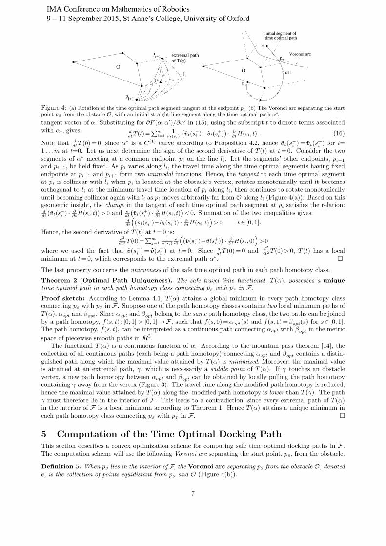
Figure 4: (a) Rotation of the time optimal path segment tangent at the endpoint pi. (b) The Voronoi arc separating the startpoint pS from the obstacle O, with an initial straight line segment along the time optimal path α∗.

tangent vector of α. Substituting for ∂F (α, α′)/∂α′ in (15), using the subscript t to denote terms associatedwith αt, gives: d

dtT (t)=

∑mi=1

1νt(si)

(vt(s

−i )−vt(s

+i )

)· ∂∂tH(si, t). (16)

Note that ddtT (0)= 0, since α∗ is a C(1) curve according to Proposition 4.2, hence vt(s

−i )= vt(s

+i ) for i=

1 . . .m at t=0. Let us next determine the sign of the second derivative of T (t) at t=0. Consider the twosegments of α∗ meeting at a common endpoint pi on the line li. Let the segments’ other endpoints, pi−1

and pi+1, be held fixed. As pi varies along li, the travel time along the time optimal segments having fixedendpoints at pi−1 and pi+1 form two unimodal functions. Hence, the tangent to each time optimal segmentat pi is collinear with li when pi is located at the obstacle’s vertex, rotates monotonically until it becomesorthogonal to li at the minimum travel time location of pi along li, then continues to rotate monotonicallyuntil becoming collinear again with li as pi moves arbitrarily far from O along li (Figure 4(a)). Based on thisgeometric insight, the change in the tangent of each time optimal path segment at pi satisfies the relation:ddt

(vt(s

−i ) · ∂

∂tH(si, t)

)> 0 and d

dt

(vt(s

+i ) · ∂

∂tH(si, t)

)< 0. Summation of the two inequalities gives:

ddt

((vt(s

−i )−vt(s

+i )) · ∂

∂tH(si, t)

)> 0 t∈ [0, 1].

Hence, the second derivative of T (t) at t=0 is:d2

dt2T (0)=

∑mj=1

1ν(si)

ddt

((v(s−i )−v(s+i )

)· ∂∂tH(si, 0)

)> 0

where we used the fact that v(s−i )= v(s+i ) at t=0. Since ddtT (0)= 0 and d2

dt2T (0)> 0, T (t) has a localminimum at t=0, which corresponds to the extremal path α∗. �The last property concerns the uniqueness of the safe time optimal path in each path homotopy class.

Theorem 2 (Optimal Path Uniqueness). The safe travel time functional, T (α), possesses a uniquetime optimal path in each path homotopy class connecting pS with pT in F .

Proof sketch: According to Lemma 4.1, T (α) attains a global minimum in every path homotopy classconnecting pS with pT in F . Suppose one of the path homotopy classes contains two local minimum paths ofT (α), αopt and βopt. Since αopt and βopt belong to the same path homotopy class, the two paths can be joinedby a path homotopy, f(s, t) : [0, 1]× [0, 1]→F , such that f(s, 0)=αopt(s) and f(s, 1)=βopt(s) for s∈ [0, 1].The path homotopy, f(s, t), can be interpreted as a continuous path connecting αopt with βopt in the metric

space of piecewise smooth paths in IR2.The functional T (α) is a continuous function of α. According to the mountain pass theorem [14], the

collection of all continuous paths (each being a path homotopy) connecting αopt and βopt contains a distin-guished path along which the maximal value attained by T (α) is minimized. Moreover, the maximal valueis attained at an extremal path, γ, which is necessarily a saddle point of T (α). If γ touches an obstaclevertex, a new path homotopy between αopt and βopt can be obtained by locally pulling the path homotopycontaining γ away from the vertex (Figure 3). The travel time along the modified path homotopy is reduced,hence the maximal value attained by T (α) along the modified path homotopy is lower than T (γ). The pathγ must therefore lie in the interior of F . This leads to a contradiction, since every extremal path of T (α)in the interior of F is a local minimum according to Theorem 1. Hence T (α) attains a unique minimum ineach path homotopy class connecting pS with pT in F . �

5 Computation of the Time Optimal Docking PathThis section describes a convex optimization scheme for computing safe time optimal docking paths in F .The computation scheme will use the following Voronoi arc separating the start point, pS, from the obstacle.

Definition 5. When pS lies in the interior of F, the Voronoi arc separating pS from the obstacle O, denotede, is the collection of points equidistant from pS and O (Figure 4(b)).

7

IMA Conference on Mathematics of Robotics 9 – 11 September 2015, St Anne’s College, University of Oxford

The following lemma specifies the shape of the safe time optimal path between pS and the Voronoi arc.

Lemma 5.1. Starting with zero speed at pS, the safe time optimal path forms a straight line between pS

and the Voronoi arc separating pS from the obstacle O.

Proof sketch: Consider the safe time optimal path α∗ starting with zero speed at pS. Let pe be thecrossing point of α∗ with the Voronoi arc e. Since α∗ is a local minimum of T (α), the portion of α∗ betweenpS and pe is also a local minimum of T (α), with respect to paths which start with zero speed at pS and reachpe. The robot’s initial braking safety distance at (pS, 0) satisfies d(ν)= ν2/2amax =0. Hence, if pS is notlocated on the obstacle’s boundary, d(ν)< dst(pS, O), and the uniform braking safety constraint is initiallyinactive. The robot can therefore safely use its maximal acceleration, amax, in order to gain as much speedas possible. Accelerating with amax along the straight line connecting pS and pe ensures maximal attainablespeed along the shortest path connecting pS with pe. The straight line segment is therefore time optimal,and hence forms the portion of α∗ between pS and pe. �The computation scheme focuses on the piecewise time optimal paths connecting pS and pT . These pathsconsist of a straight line segment leading from pS to the Voronoi arc, followed by time optimal path segmentsin each proximity cell (Section 3). The crossing points of these paths with the Voronoi arc and proximity cellboundary lines will serve as the optimization variables. The computation starts with a selection of a particularpath homotopy class connecting pS and pT in F , associated with a sequence of m + 1 proximity cells withboundary lines l1, . . . , lm. The crossing points along e and l1, . . . , lm are parametrized by p(u0) : [0, 1]→ e andp(ui) : [0, 1]→ li for i=1 . . .m (Figure 5(a)). Since each time optimal path segment is uniquely determined byits two endpoints, the safe travel time functional, T (α), becomes a function of the crossing point parametersu0, u1, . . . , um. Computation of the safe time optimal path connecting pS and pT is next performed in theset (u0, . . . , um)∈ [0, 1]× · · · × [0, 1], based on the following monotonicity property of T (α).

Proposition 5.2 ([11]). Let α(u0, . . . , um) parametrize the piecewise time optimal paths connecting pS and pT

in F , while crossing the Voronoi arc e and the proximity cell boundary lines l1, . . . , lm. Let u∗ =(u∗0, . . . , u

∗m)

be the parameter values of the optimal crossing points. The functional T (α(u0, . . . , um)) is monotonicallyincreasing along any ray emanating from u∗ in the set (u0, . . . , um)∈ [0, 1]× · · · × [0, 1].

Since T (α(u0, . . . , um)) is monotonically increasing along rays emanating from (u∗0, . . . , u

∗m), its level sets form

star shaped sets in the set (u0, . . . , um)∈ [0, 1]× · · · × [0, 1].2 This property is illustrated in Figure 5, whichplots the contours of T (α(u0, u1)), for the piecewise time optimal paths passing through two crossing points,p(u0) and p(u1). The contours form convex sets (and hence star shaped sets) in the (u0, u1) plane, withcenter point at the optimal parameter values (u∗

0, u∗1).

Convex optimization algorithms require that the level sets of T (α(u0, . . . , um)) be convex. However, thesame algorithms can be applied when the level sets are star shaped with a common center point at the optimalparameter values u∗. This observation is based on the relation ∇T (α(u)) ·(u−u∗)≥ 0 satisfied by star shapedlevel sets, which allows construction of a barrier function (or a bounding ellipsoid) in each iteration of theconvex optimization process. Standard convex optimization algorithms run in O(m3 log(R/ϵ)) time [13],where m is the number of crossing points, R is the travel time difference between the initial path and theexact solution, and ϵ is the desired solution accuracy. The total number of crossing points is upper boundedby the number of obstacle features, n, and the convex optimization therefore runs in O(n3 log(R/ϵ)) time.

6 Computation ExampleThis section describes a safe time optimal docking path example, depicted in Figure 6(a). The mobile robotis modeled a point moving with amax =0.5 m/sec2, which is typical for autonomous robots operating inwarehouse environments. The example describes docking maneuvers around a rectangle obstacle corner.The obstacle is of size is 15× 30 meters, with vertices at (0, 0), (30, 0), (30,−15), and (0,−15) in the (x, y)plane. The start point is located at pS =(10, 10). Figure 6(a) depicts three time optimal docking paths, α1,α2, and α3, associated with targets located on the obstacle’s boundary at pT1 =(5, 0), pT2 =(0,−7.5), andpT3 =(10,−15). The initial path in each computation started with a straight line segment connecting pS witha point on the Voronoi arc, followed by time optimal segments connecting the obstacle vertices leading tothe respective target. The computation resulted in the time optimal docking paths depicted in Figure 6(a),with T (α1)= 8.2, T (α2)= 17.1, and T (α3)= 27.8 seconds.

Importantly, the time optimal solutions specify the geometric shape of the docking paths as well as the

2A set S in IRm is star shaped when there exists a center point, p0 ∈S, such that every point p∈S lies on a unique rayemanating from p0.

8

IMA Conference on Mathematics of Robotics 9 – 11 September 2015, St Anne’s College, University of Oxford

10 10.5 11 11.5 12 12.5 13 13.5 1410

10.5

11

11.5

12

12.5

13

13.5

14

0u

1u

*0u

*1u

*1u

*0u

(a) (b)

* *0 1( , )u u

O0u

1u

optimal path

Sp

Tp

voronoi arc

proximity cell

boundary lines

*a

Figure 5: (a) Parametrization of the piecewise time optimal paths connecting pS and pT by (u0, u1). (b) Contours ofT (α(u0, u1)) in the (u0, u1) plane.

robot at start

position

voronoi arc

proximity cell

boundary lines

O1Tp

2Tp

3Tp

x

y

1a

2a

3a

(a)

0 10 20 30 40 50 600

0.5

1

1.5

2

2.5

3

path length [m]

[ / sec]v marrival to

voronoi arc

1a

2a 3

a

(b)Figure 6: (a) Three time optimal docking maneuvers around an obstacle corner. (b) The robot’s speed plotted as a functionof the path length parameter s.

speed profile along these paths. The robot’s speed along each path, ν(s), is plotted as a function of the pathlength parameter, s, in Figure 6(b). Note that each path starts with maximal acceleration along the straightline segment leading to the Voronoi arc. The robot next gradually decreases its speed until docking at thetarget, with maximal deceleration attained in the final approach to the obstacle’s boundary.

7 ConclusionThe paper considered the synthesise of safe time optimal paths for a mobile robot docking at targets locatedon a polygonal obstacle boundary. Starting with zero speed, the robot is required to approach a dockingtarget with zero final speed, while maintaining a speed dependent circular safety zone centered at therobot’s current position. The safe travel time functional, T (α), was formulated and its basic propertieswere described. The paper next established that time optimal docking paths always start with a straightline segment leading to the Voronoi arc separating between the start point and the obstacle. Monotonicityof T (α) over the piecewise time optimal paths in each path homotopy class of the environment lead toan efficient convex optimization scheme executed over the piecewise time optimal paths, with optimizationvariables consisting of the paths’ crossing points locations on the Voronoi arc and boundary lines betweenproximity cells induced by the obstacle’s geometric features.

As demonstrated in simulation examples, the solutions specify the geometric shape of the time optimaldocking paths, as well as the speed profile along these paths. This feature provides a significant progress withrespect to classical configuration-space path planning approaches, which only generate collision avoidingpaths without any consideration of the robot’s speed during the path planning process. Moreover, thegeometric shape of the safe time optimal docking paths is invariant with respect to the robot’s maximaldeceleration, amax. Hence, while the actual travel time along the safe time optimal paths is a systemdependent parameter, the geometric shape of the safe time optimal docking paths depends only on thelocation of the start and target relative to the obstacle.

An important extension concerns the generalization of the circular braking safety zone into a headingdependent safety zone. For instance, when a mobile robot travels with high speed in a long narrow corridor,a non-circular safety zone aligned with the corridor’s axis will allow the robot significantly higher speedsthan the conservative circular safety zone. This extension would require planning in the mobile robot’sfour-dimensional position and velocity space, and we hope to report initial results in the near future.

9

IMA Conference on Mathematics of Robotics 9 – 11 September 2015, St Anne’s College, University of Oxford

References[1] Traffic jam assistance. Volvo Car Group. www.media.volvocars.com/global, 2013.

[2] O. Brock and O. Khatib. High-speed navigation using the global dynamic window approach. In IEEEInt. Conf. on Robotics and Automation, pages 341–346, 1999.

[3] H. Choset, K. M. Lynch, S. Hutchinson, G. Kantor, W. Burgard, L. E. Kavraki, and S. Thrun. Principlesof Robot Motion. MIT Press, 2005.

[4] P. Fiorini and Z. Shiller. Motion planning in dynamic environments using velocity obstacles. Int. J. ofRobotics Research, 17(7):760–772, 1998.

[5] D. Fox, W. Burgard, and S. Thrun. The dynamic window approach to collision avoidance. RoboticsAutomation Magazine, IEEE, 4(1):23 –33, 1997.

[6] T. Fraichard. A short paper about motion safety. In IEEE Int. Conf. on Robotics and Automation,pages 1140–1145, 2007.

[7] I. M. Gelfand and S.V. Formin. Calculus of Variations. Prentice-Hall, 1963.

[8] S. Karaman and E. Frazzoli. Sampling-based algorithms for optimal motion planning. The Int. J. ofRobotics Research, 30(7):846–894, 2011.

[9] F. Large, D. Vasquez, T. Fraichard, and C. Laugier. Avoiding cars and pedestrians using velocityobstacles and motion prediction. In IEEE Intelligent Vehicle Symp., pages 375–379, 2004.

[10] S. M. Lavalle. Rapidly-exploring random trees: A new tool for path planning. Technical report, Dept.of Computer Science, Iowa State University, 1998.

[11] G. Manor. Autonomous Mobile Robot Navigation With Velocity Constraints. PhD thesis, TechnionIsrael Inst. of Technology, Haifa, Israel, http://robots.technion.ac.il/publications, 2014.

[12] J. Markoff. Google cars drive themselves in traffic. New York Times, October 2010.

[13] Y. E. Nesterov and A. S. Nemirovsky. Interior Point Polynomial Methods in Convex Programming:Theory and Applications. Springer Verlag, New York, 1992.

[14] L. Nirenberg. Variational and topological methods in nonlinear problems. Bulletin of the AMS, 4(3):267–302, 1981.

[15] I. Sherr and M. Ramsey. Toyota and Audi move closer to driverless cars, January 2013.

[16] Z. Shiller, S. Sharma, I. Stern, and A. Stern. Online obstacle avoidance at high speeds. Int. J. ofRobotics Research, 32:1030–1047, 2013.

[17] J. Snape, J. van den Berg, and S. J. Guy. The hybrid reciprocal velocity obstacle. IEEE Trans. onRobotics, 27(4):696–706, 2011.

[18] P. R. Wurman, R. D’Andrea, and M. Mountz. Coordinating hundreds of cooperative, autonomousvehicles in warehouses. AI Magazine, 29:9–19, 2008.

10

IMA Conference on Mathematics of Robotics 9 – 11 September 2015, St Anne’s College, University of Oxford