Prepared for submission to JHEP

Subatomic Physics: the Notes1

C.P. Burgess

Department of Physics & Astronomy, McMaster University

and Perimeter Institute for Theoretical Physics

1 c©Cliff Burgess, for Physics 4E03 Winter Term 2016

Contents

1 The story so far... 2

1.1 Prequel: more than just atoms 2

1.2 Units and scales 11

1.3 Relativistic kinematics 14

2 Calculational tools I 23

2.1 Conserved quantities 23

2.2 Decays: general properties 25

2.3 Scattering: general properties 38

3 Calculational tools II 48

3.1 Classical two-body scattering 48

3.2 Quantum potential scattering 57

3.3 Perturbation theory and the Born approximation 71

4 Nucleon substructure 78

4.1 Electrons, nucleons and quarks 79

4.2 Elastic scattering 84

4.3 Inelastic ep scattering 88

5 Nuclear structure 92

5.1 Inter-nucleon interactions 93

5.2 Nuclear models 98

5.3 Isospin and meson exchange 108

5.4 Radioactivity 115

6 Quantum Field Theory 127

6.1 Heisenberg’s harmonic oscillator 128

6.2 Creation and annihilation operators 130

6.3 Interactions and fields 134

6.4 Relativistic quantum field theory 137

6.5 Bosons and forces 141

7 The Standard Model 143

7.1 Fermions and the generation puzzle 143

7.2 Bosons and the four forces 145

7.3 Where the Standard Model fails 148

– 1 –

A major theme of 20th Century physics is that we are surrounded by substructure: what

we see around us is built from smaller (often initially invisible) constituents and much of

the diversity we see can be efficiently understood as consequences of the properties of these

constituents. Furthermore this is a recursive process, with the constituents themselves often

built from still-smaller pieces: matter is made of molecules; molecules are made of atoms;

atoms made of nuclei and electrons; nuclei are built from nucleons (i.e. protons and neutrons);

nucleons are made of quarks and gluons; and so on.

Subatomic physics is the part of this story starting with nuclei and continuing on to the

smallest constituents known. We call particles ‘elementary’ if they have no substructure so far

as we can tell, and at present the list of such particles contains around 20 entries. The theory of

these particles and their mutual interactions is called the Standard Model and works extremely

well (with a few noteworthy exceptions). But history teaches us that this classification of the

elementary is at best provisional and may be changed in light of later evidence with finer

resolution. These notes summarize the evidence for the present picture, as well as the flaws it

is known to have, at a level appropriate for upper-year physics undergraduates. The reader is

assumed to be familiar with non-relativistic quantum mechanics, electromagnetism and the

rudiments of special relativity.

1 The story so far...

This section contains some preliminary background information needed to tell this story, and

starts by summarizing the first indications that there might be an interesting story to tell.

1.1 Prequel: more than just atoms

The first discovery of the particles we now still regard as elementary occurred during the

closing years of the 19th century. Many of these developments arose as unintended conse-

quences of the discovery of cathode rays that are the result of applying a high voltage to a

small amount of gas inside an otherwise evacuated tube. A very practical tube for producing

these rays — called a Crookes tube — was developed as early as 1875. The presence of the

cathode rays was inferred because they caused the gas in the tube (or any florescent material

on the glass wall of the tube) to glow. (This is the phenomenon on which florescent lights

and televisions were based until very recently).

We now know what happens with these tubes. The applied high voltage strips electrons

from the gas atoms and the free electrons (i.e. the cathode rays) then are repelled by the

negative cathode and flow towards the positive anode. Similarly, the leftover positive ions (or

‘anode’ rays) drift from the positive anode towards the cathode. The florescence is caused by

collisions with these rays exciting gas atoms which emit light as they de-excite.

– 2 –

Figure 1. A Crookes tube with (bottom panel) and without (top panel) voltage applied, showing

the florescense caused by the cathode rays when power is applied. The shadow of an obstacle shaped

like a Maltese cross is visible and shows that the rays travel in straight lines. (Figure source: Wikipedia

https://en.wikipedia.org/wiki/Crookes tube).

1.1.1 X rays

Many of the early workers with Crookes tubes (including Crookes himself, apparently) no-

ticed that photographic plates became fogged up if they were near the tube when it was in

use. Roentgen was the first to investigate in detail why this occurred, and by performing

experiments with various objects between the tube and the plates found that images could

be made of the dense parts within otherwise opaque objects. He determined that the plates

were fogged because they were being exposed to some new rays he called x-rays. By showing

they moved in straight lines even in the presence of magnetic fields he showed these rays were

electrically neutral.

We now know x-rays to be photons that are somewhat more energetic than visible or UV

photons, and are emitted (like the florescent light) when excited electrons drop down into a

state very close to the nucleus.

1.1.2 Radioactivity

In 1896 Becquerel, in Paris, ran experiments seeking to determine whether florescent materials

could be made to emit x-rays through exposure to sunlight. To this end he took a good

florescent compound, wrapped it in dark paper and placed it next to a photographic plate,

intending to expose it to sunlight. Although his plans were thwarted when it was overcast in

Paris that day, he nevertheless developed the plate and unexpectedly found that it had been

exposed.

On further experimenting he determined that the exposure was due to the spontaneous

– 3 –

emission of rays by the florescent material itself (rather than due to their florescing), since

the photographic plates would become fogged regardless of whether or not the material was

exposed to light or not. Furthermore, he found the rays responsible to be electrically charged

since their path could be deflected by applying a magnetic field.

Figure 2. A schematic of how the paths of various radioactive rays respond to magnetic fields. The

magnetic field points perpendicular to the page and is represented by the grid of dots. γ rays do not

bend while α and β rays bend in opposite directions (because the particles involved have opposite-sign

charges). β rays bend more strongly because their charge-to-mass ratio, q/m, is much larger. (Figure

source: http://www.particleadventure.org/radio part.html).

Over time it became clear that there are actually three different types of radioactive rays,

called α, β and γ rays. Each responds differently to a magnetic field, with α rays behaving

like positively charged particles, β rays behaving like negatively charged particles and γ rays

behaving like electrically neutral particles (and so are not deflected by magnetic fields). We

now know what these ‘rays’ really are:

• α rays are made up of α particles, which are nuclei of 4He — that is, two neutrons and

two protons bound together. (Here the convention is that the left-superscript ‘4’ of 4He

counts the total number of protons and neutrons present in the nucleus.) These types

of Helium nuclei are particularly tightly bound and so very stable, and under certain

circumstances can escape as a group from much larger nuclei. (In Becquerel’s case it

was the Uranium contained in his florescent compound that was responsible.)

• β rays consist of very energetic electrons that can be produced within the nucleus,

usually through the decay of a neutron into a proton plus an electron (plus another

particle, called an antineutrino — more about which later) through the reaction1 n→p+ + e− + νe.

1When ± or 2± or 3± appears as a superscript for a particle label it represents the particle’s electric charge

– 4 –

• γ rays are very energetic photons that differ from x-rays only by having more energy.

1.1.3 The electron

The nature of the cathode rays themselves was initially confused because of early experiments

that incorrectly indicated that they were not deflected by magnetic fields (and so must be

electrically neutral). (In retrospect these experiments were wrong because they were not able

to get a good enough vacuum in the tube, and as a result ionization of the gas partially

shorted out the voltage being applied to generate the electric field being used to test for

a charge.) The situation was definitively settled in 1897 in experiments performed by J.J.

Thompson, who was able to get a good enough vacuum in his apparatus to show that cathode

rays are bent by a magnetic field, and in a direction that corresponds to being oppositely

charged relative to α particles.

(a) No magnetic field (b) Magnetic field applied

Figure 3. A Crookes tube with a no magnetic field applied (left panel) and with a magnetic field

(right panel), showing how magnetic fields deflect cathode rays and so move the image of the Maltese

cross on the florescent screen. (Figure source: Wikipedia https://en.wikipedia.org/wiki/Crookes tube).

Furthermore, he used a clever combination of electric and magnetic fields to eliminate

experimental unknowns and thereby pin down the charge-to-mass ratio of cathode rays. To

do so Thompson produced cathode rays in the tube and deflected them by applying an electric

field, as shown in Fig. 4.

He assumed the cathode ray was made of particles with mass m and charge q (this sounds

uncontroversial to us, but at the time cathode rays were widely thought to be ‘disturbances

in the aether’), and that they are emitted from the cathode with speed v0. By applying a

in units of the proton charge, e. Hence p or p+ is the proton and e− is the electron. The superscript is often

omitted for protons, as well as for neutral particles like neutrons (unless making a distinction with another

particle with the same symbol: e.g the particle π0 as opposed to π+ or π−).

– 5 –

Figure 4. Thompson’s apparatus for identifying the charge-to-mass ratio of cathode rays. High

voltage is applied at the terminals marked + and − causing cathode rays to be emitted from the

cathode marked C. The rays are collimated by passing through slits S1 and S2 to form a beam

whose position can be seen on a florescent screen AO. Another voltage is applied between plates P1

and P2, forming an electric field in between that deflects the beam direction. Three sample beam

trajectories are drawn, with the middle one corresponding to no voltage between P1 and P2 and the

other two (coloured) trajectories corresponding to electric fields in opposite directions. (Figure source:

http://web.calstatela.edu/faculty/kaniol/f2000 lect nuclphys/lect1/thompson electron.htm).

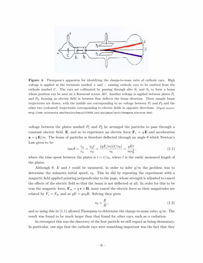
voltage between the plates marked P1 and P2 he arranged the particles to pass through a

constant electric field, E, and so to experience an electric force Fe = qE and acceleration

a = qE/m. The beam of particles is therefore deflected through an angle θ which Newton’s

Law gives to be

tan θ =vyvx

=ayt

v0=

(qE/m)(`/v0)

v0=qE`

mv20

, (1.1)

where the time spent between the plates is t = `/v0, where ` is the easily measured length of

the plates.

Although θ, E and ` could be measured, in order to infer q/m the problem was to

determine the unknown initial speed, v0. This he did by repeating the experiment with a

magnetic field applied pointing perpendicular to the page, whose strength is adjusted to cancel

the effects of the electric field so that the beam is not deflected at all. In order for this to be

true the magnetic force, Fm = q v×B, must cancel the electric force so their magnitudes are

related by Fe = Fm and so qE = qv0B. Solving then gives

v0 =E

B, (1.2)

and so using this in (1.1) allowed Thompson to determine the charge-to-mass ratio, q/m. The

result was found to be much larger than that found for other rays, such as α radiation.

In retrospect this was the discovery of the first particle we still regard as being elementary.

In particular, one sign that the cathode rays were something important was the fact that they

– 6 –

are universal: they always have the same value of q/m regardless of the kind of dilute gas

that is used in the tube. The same is not true of the ‘anode’ rays, which are the positively

charged particles that are repelled by the anode and move towards the cathode. Anode rays

are produced when Crookes tubes are set up with the voltages reversed, so that the source

electrode at the left of above diagram is positively charged rather than negatively charged.

When this is done the value of q/m found for these rays is much smaller than for cathode

rays and, more importantly, has a value that depends on the precise gas used in the tube.

In retrospect what we now know is that applying a large enough voltage strips electrons

from the atoms of the rarefied gas, after which the negative electrons are repelled by the

cathode (and so are the cathode rays) while the positive ions are repelled by the anode

(and so make up the anode rays). The fact that cathode rays always look the same is now

understood because all atoms consist of electrons orbiting a nucleus, and although different

elements have different nuclei (and so differing numbers of electrons in orbit) they are all built

using the same type of electron.

1.1.4 The nucleus

Having discovered the electron, and that electrons can be extracted from neutral atoms,

Thompson was led to speculate about what the structure of the atom might be. In the absence

of a better idea (and with the required tools like quantum mechanics not yet developed) he

proposed the ‘plum-pudding’ model of the atom. In this model the atom is imagined to

be a blob of positive charge (of unknown structure) within which electrons were uniformly

distributed like the raisins in a pudding.

To test this model Rutherford performed an experiment in which he bombarded a thin

gold foil with α particles that he obtained from the decay of a radioactive source. The idea

was to watch how the alpha particles were scattered by the electrons and the positive charge

within the atom, and use this to infer how they might be distributed. The apparatus is as

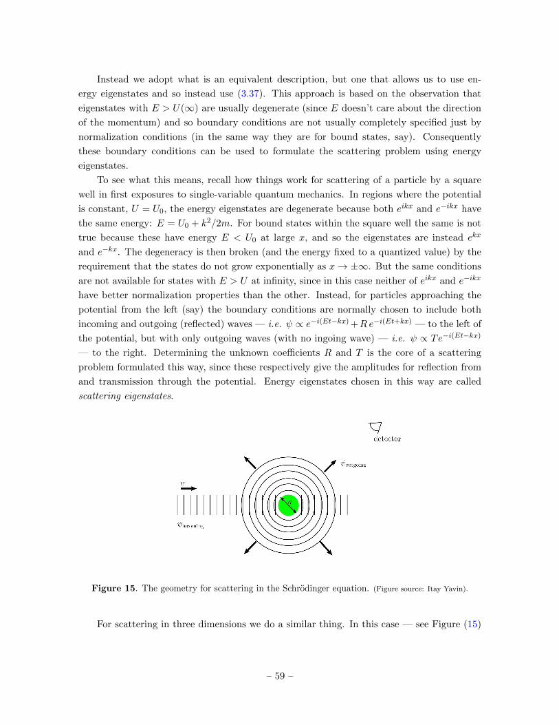
illustrated in Fig. 5.

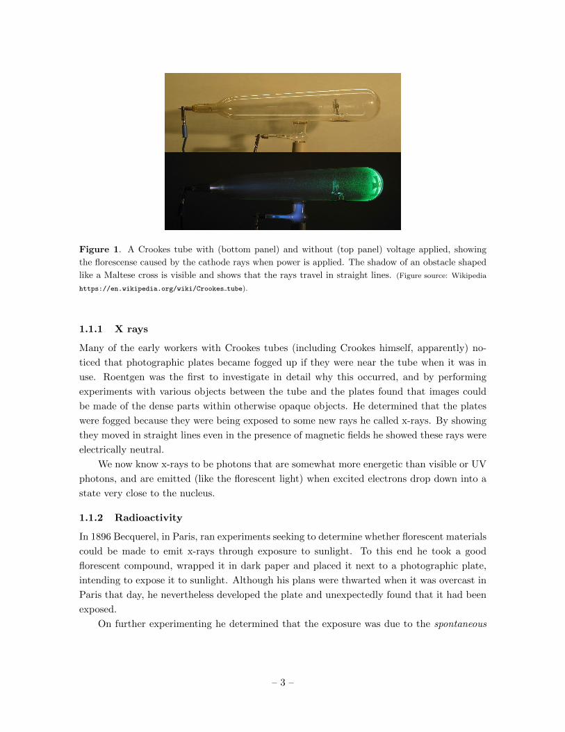
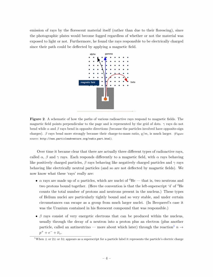
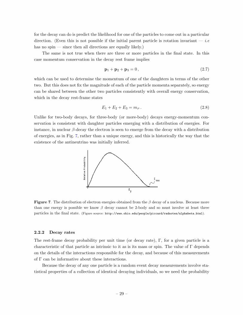
Figure 5. Schematic illustration of the apparatus with which Rutherford intended to probe the

structure of the atom and test the plum-pudding model. The zinc-sulphide coated screen floresces

when hit by α particles and so allows the direction of the scattered beam to be measured. (Figure

source: Boston University http://physics.bu.edu/cc104/chapters10and11.html).

– 7 –

By this time the electric charge of the electron had been measured (through the Millikan

oil-drop experiment of 1909) and so it was known that the electron had a charge equal in

size to (but opposite in sign from) the charge, q = e, of the Hydrogen ion (what we now

call the Hydrogen nucleus, or proton). The measurement of q/m for each then implied the

electron was 1836 times lighter than a proton, and so that α particles were much heavier

than electrons. As a result an α particle was expected only to scatter through a small angle,

if at all, when encountering an electron. The same would also be true for scattering from

a distributed positive charge distribution (as we see in detail in a later section), leading to

the expectation that a plum-pudding atom would give the result illustrated in the left-hand

panel of Fig. 6.

The experimental results therefore came as something of a surprise: while many alpha

particles did only scatter through small angles some scattered much more strongly, even

recoiling back into the same hemisphere from which they initially came (see the right-hand

panel of Fig. 6). Furthermore, the measured probability of scattering as a function of the angle

of the outgoing α-particle relative to its initial direction was consistent with that expected

for scattering from the Coulomb potential of a point charge (more about this distribution

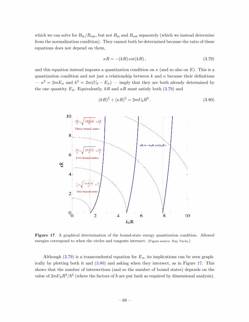
below). Although Rutherford did not know the charge of a gold atom he thought it was likely

to be roughly half its atomic weight, and so Q ' 100 e. For this charge he could calculate

the point of closest approach to the atom’s central charge and so could put an upper limit on

the size of the charge distribution to be rN <∼ 10−14 m. This was already known to be much

smaller than the radius, rA ∼ 10−10 m, of the gold atom.

(a) Plum-pudding result (b) Nuclear result

Figure 6. Schematic illustration of the difference between what would be found in Rutherford’s

experiment if the plum-pudding model were true (left panel) and what was actually found (indicating

the presence of a very compact source of positive charge – i.e. the nucleus. (Figure source: Boston

University http://physics.bu.edu/cc104/chapters10and11.html).

This set the stage for the development of atomic physics and quantum mechanics. Atoms

became understood to consist of Z electrons (each with charge −e) orbiting a nucleus with

charge Z e and mass M where M = Am0 + δ is close to an integer times the atomic mass

unit, m0. Here δ can be negative but small: |δ| m0 where m0 is roughly the mass of a

– 8 –

proton. (In practice m0 is usually taken to be 112 the mass of a Carbon nucleus, since this

is better measured.) The positive integer Z is called the atom’s atomic number or nuclear

charge and the positive integer A is called its atomic mass number or atomic weight.

We now know the nucleus to be a bound state built out of a total of Z protons and

N = A− Z neutrons (both of whose masses are similar to m0), and so the difference δ is to

do with the binding energy that is responsible for holding the protons and neutrons together.

Because protons each carry charge e and neutrons are neutral the nuclear charge is Q = Z e,

and this determines the number of electrons needed to make the total atom neutral. Because

chemical properties depend on the number of these electrons the number Z determines which

element the atom corresponds to.

Although all atoms for any element share the same value of Z, they may differ in the

number of neutrons present in their nucleus (and so differ also in their value for A). These

different isotopes of an element are represented by AX (where X is the symbol for the element

— e.g. He for Helium or W for Tungsten, and the superscript A is the isotope’s atomic

weight). When the value of the nuclear charge is meant to be emphasized explicitly it can

also be put in as a left-subscript,2 as in AZX. For example 12C or 12

6C represents the most

common isotope of Carbon whose nucleus contains 6 protons and 6 neutrons, while 14C or14

6C represents a radioactive isotope of Carbon whose nucleus holds 6 protons but 8 neutrons.

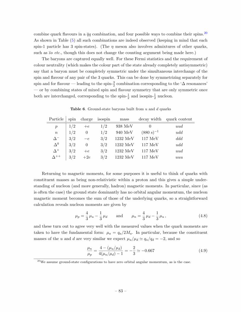
1.1.5 The proton and neutron

Besides discovering the nucleus, Rutherford also pointed the way towards many experiments

that followed since much would be learned about the structure of nuclei and their constituents

by colliding them with other particles at high energies and studying what comes out. In the

early days the particle beams used to probe the structure of atoms were α-particles coming

from radioactive decays. Included amongst the discoveries arrived at in this way was the

discovery of the particles we now know to be the constituents of atomic nuclei: protons and

neutrons.

Protons were discovered to be nuclear constituents in experiments performed, again by

Rutherford, in 1917 (but reported in 1919). In these Rutherford studied the inelastic3 (and

first ever man-made) nuclear reaction

α+ 147N→ 17

8O + p , (1.3)

by bombarding air with α particles. He determined that after the bombardment the air con-

tained traces of Hydrogen that had not been previously present, and (rightly) concluded that

he had knocked a Hydrogen nucleus out of one of the atomic nuclei. (It was the accumulation

2This notation leaves the right superscript free to indicate the ionic charge, should the nucleus not be

surrounded by a full complement of electrons.3A reaction is inelastic if the initial and final kinetic energies are not equal, so some internal energy is either

absorbed or released.

– 9 –

of traces of Helium outside of radioactive materials that similarly led to the conclusion that

α particles were Helium nuclei.) The emerging proton was later seen more directly when the

reaction took place within a cloud chamber, which is an early detector that allowed the direct

measurement of the track of a quickly moving charged particle.

Since this discovery showed that nuclei could emit protons and β decays showed that

nuclei could emit electrons it was natural to guess that nuclei were somehow built from

protons and electrons. And because protons and electrons were known to carry equal but

opposite electric charges, and protons were much more massive than electrons, the proper

nuclear charge, Z, and mass number, A, could be achieved if nuclei could somehow be built

from A = Z+N protons plus N electrons, since this would ensure an atomic charge of Z and

an atomic mass number of A.

Several things undermined this proposal in the end. First, nobody had a good explanation

of the forces that would be required to bind protons and electrons into nuclei in this way. But

this was not too daunting before the discovery of quantum mechanics because nobody then

could understand how electrostatic attraction between electrons and protons could explain

the orbits of electrons in an atom either. The discovery of quantum mechanics in the 1920s

then resolved the problem of understanding how electrons move within atoms, but contrary

to expectations it did not also in itself resolve the riddle of nuclear structure.

Quantum mechanics specifically undermined the idea that electrons and protons could

bind within a nucleus in several ways. First, because both electrons and protons are fermions

this model predicts that nuclei should satisfy Bose statistics whenever N = A − Z is even,

and should satisfy Fermi statistics whenever N is odd. In 1929 this ran into trouble once the

vibrational spectrum of the Nitrogen molecule was measured. The 14N nucleus has charge

Z = 7 and mass A = 14 and so was expected to consist of 14 protons plus 7 electrons and

therefore be a fermion. Yet observations instead showed that the statistical weights for the

energy levels of the Nitrogen molecule required the wave-function to be symmetric under

interchange of the Nitrogen nuclei: that is these nuclei behave as bosons. (More generally,

observations show that nuclei are fermions whenever A is odd and are bosons whenever A is

even.) Furthermore, it was also realized that the uncertainty principle requires the energy

of an electron localized within something so small as a nucleus to be much higher than the

energy associated with the electrons seen to emerge from nuclei in β decays.

Exercise: Use position-momentum uncertainty relations, ∆x∆p ≥ ~/2, to es-

timate the lower limit to an electron’s momentum if it is localized within a nu-

cleus of size 1 fm = 10−15 m. Given the relativistic energy-momentum relation,

E2 = p2c2 + m2c4, and electron mass (mc2 = 511 keV) what is the electron’s

kinetic energy (Ekin = E − mc2) corresponding to this momentum? How does

this compare with the maximum electron energy (about 17 keV) seen in tritium

β decay?

– 10 –

The ingredients required to properly understand the nucleus were finally in hand once

the neutron was discovered in 1932. The discovery was just missed by Walther Bothe and

Herbert Becker who found in 1931 that α particles bombarding Boron or Lithium produced

some sort of radiation that was not bent by electric and magnetic fields. They therefore

assumed these rays were γ rays, but this was made to seem doubtful because of the discovery

by Irene Joliot-Curie and Frederic Joliot that these rays when impinging on paraffin (or other

things containing Hydrogen) caused the production of very energetic protons. In 1932 James

Chadwick, again by probing nuclei with α particles through the reaction

α+ 94Be→ 12

6O + n , (1.4)

showed that the new rays were electrically neutral particles whose mass was similar to that

of a proton. Unlike γ rays, because of their mass neutrons carry enough momentum to knock

a Hydrogen nucleus out of a sample when colliding with one, which explained the earlier

observations with paraffin.

The discovery of the neutron allowed a number of things to be understood. Besides giving

a better picture of the nucleus (more about which later), it opened the door to understanding

β decay to be the result of neutrons within the nucleus decaying into protons and electrons

(plus, it turned out, another undetected particle, the neutrino about which nothing was known

at that time).

Neutrons also provided a new probe with which to bombard other nuclei, and they are

particularly useful for this purpose (compared with protons or α particles) because their elec-

trical neutrality means they are not repelled by the target nucleus’ electric charge. Enrico

Fermi found in 1934 that stable elements could be induced to become radioactive by bom-

barding them with neutrons, and by 1938 Otto Hahn, Lise Meitner and Fritz Strassmann

discovered nuclear fission when they found that bombardment by neutrons could also split

heavy nuclei into much much smaller pieces than happens through ordinary radioactivity.

1.2 Units and scales

For future purposes it is worth recording the units used throughout the rest of the notes.

1.2.1 Electron-Volts

Historically, the prominent role played by cathode rays made the electron-Volt a natural unit

of energy:

An electron-Volt (or eV for short) is defined as the energy acquired by an electron

falling through a voltage difference of one Volt, which implies 1 eV = 1.602176565×10−19 J.

The usual metric conventions apply for multiples of this unit: 1 meV = 10−3 eV, 1 keV =

103 eV, 1 MeV = 106 eV, 1 GeV = 109 eV, 1 TeV = 1012 eV, and so on.

– 11 –

1.2.2 Fundamental units

Another convenient choice is to use units so that the main fundamental constants of nature

are set to unity: i.e. choose units of length, time and temperature so that all three of the

(reduced) Planck constant, speed of light and Boltzmann constant satisfy ~ = c = kB = 1.

If this is done then it is no longer necessary to keep track of factors of these constants in

expressions, which helps declutter formulae and makes it easier to see which variables are the

important ones.

Once these units are used then we can measure any physical quantity in terms of a unit

of length, say. (We could equally express everything in terms of a unit of time, or in terms of

a unit of energy.) That is, if we say a time interval is measured in meters: ∆t = 3 m, what

we mean is that the time corresponds to how long it takes light to travel 3m, so there is an

implicit unwritten factor of c = 1. The result in seconds can be found from ∆t = 3 m/c =

(3 m)/(3.0 × 108 m/s) = 10−8 s. The required power of c (or ~ or kB) can be found using

dimensional analysis. These units only make sense because everybody agrees on the values

of c, ~ and kB. The same argument allows mass to be written in units of energy where what

is really meant by m = 27 J is m = (27 J)/c2 = (27 J)/(3.0× 108 m/s)2 = 3.0× 10−15 kg.

Similarly the universal constant ~ = 1.1×10−34 J-s allows energy to be converted to units

of inverse seconds (or for time to be measured in units of inverse Joules). That is, we can

arrange that ~ = 1 (i.e. use natural units) if we measure energy in units of s−1 = 1.1× 10−34

J. If someone tells us in natural units that E = 80 s−1 then dimensional analysis tells us that

there is an implicit, unwritten factor of ~ = 1 and so to get the energy in Joules we write

E = 80 s−1 × ~ = (80 s−1)(1.1× 10−34 J s) = 8.8× 10−33 J.

Because ~ has dimensions of (energy) × (time) it follows that ~c = 3.3 × 10−26 J-m

has dimensions (energy) × (distance). This allows us to measure energy in inverse metres

(or length in inverse Joules). For instance, the appropriate power of ~c = 1 that allows

a statement like E = 42 m−1 to make dimensional sense is E = (42 m−1)~c and so E =

(42 m−1)(3.3× 10−26 J m) ' 1.4× 10−24 J.

Finally, we set kB = 1.4× 10−23 J/K to unity by agreeing to measure energy in degrees

K or (more commonly) by measuring temperature in units of energy. In particular the choice

made with fundamental units is to define the Joule as a unit of temperature so that 1 degree

K equals 1.3807 × 10−23 J, since this ensures that kB = 1. To convert temperature in J to

temperature in K we just divide by kB: e.g. T = 280 J in fundamental units really means

the temperature in K is given by T = (280 J)/kB = (280 J)/(1.4× 10−23 J/K) = 2× 1025 K.

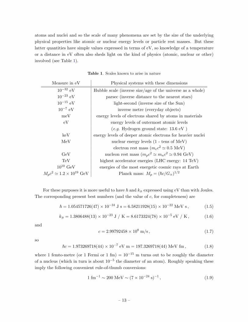
1.2.3 Hierarchies of scale

It is particularly useful to combine the above choices and so both adopt fundamental units

and express all remaining quantities in dimensions that are a power of energy, with energy

measured in electron-Volts. This is very useful because the world around us is built from

– 12 –

atoms and nuclei and so the scale of many phenomena are set by the size of the underlying

physical properties like atomic or nuclear energy levels or particle rest masses. But these

latter quantities have simple values expressed in terms of eV, so knowledge of a temperature

or a distance in eV often also sheds light on the kind of physics (atomic, nuclear or other)

involved (see Table 1).

Table 1. Scales known to arise in nature

Measure in eV Physical systems with these dimensions

10−32 eV Hubble scale (inverse size/age of the universe as a whole)

10−23 eV parsec (inverse distance to the nearest stars)

10−15 eV light-second (inverse size of the Sun)

10−7 eV inverse metre (everyday objects)

meV energy levels of electrons shared by atoms in materials

eV energy levels of outermost atomic levels

(e.g. Hydrogen ground state: 13.6 eV )

keV energy levels of deeper atomic electrons for heavier nuclei

MeV nuclear energy levels (1 - tens of MeV)

electron rest mass (mec2 ' 0.5 MeV)

GeV nucleon rest mass (mpc2 ' mnc

2 ' 0.94 GeV)

TeV highest accelerator energies (LHC energy: 14 TeV)

1010 GeV energies of the most energetic cosmic rays at Earth

Mpc2 ' 1.2× 1019 GeV Planck mass: Mp = (~c/GN)1/2

For these purposes it is more useful to have ~ and kB expressed using eV than with Joules.

The corresponding present best numbers (and the value of c, for completeness) are

~ = 1.054571726(47)× 10−34 J s = 6.58211928(15)× 10−22 MeV s , (1.5)

kB = 1.3806488(13)× 10−23 J / K = 8.6173324(78)× 10−5 eV / K , (1.6)

and

c = 2.99792458× 108 m/s , (1.7)

so

~c = 1.973269718(44)× 10−7 eV m = 197.3269718(44) MeV fm , (1.8)

where 1 femto-metre (or 1 Fermi or 1 fm) = 10−15 m turns out to be roughly the diameter

of a nucleus (which in turn is about 10−5 the diameter of an atom). Roughly speaking these

imply the following convenient rule-of-thumb conversions:

1 fm−1 ∼ 200 MeV ∼ (7× 10−24 s)−1 , (1.9)

– 13 –

and

1K ∼ 9× 10−5 eV . (1.10)

For convenience the Appendix provides several tables that convert between standard units

for various quantities and their corresponding expressions in eV. When using these units it is

useful to orient oneself by ordering several commonly occurring scales in physics as expressed

in eV, as done in Table 1.

1.3 Relativistic kinematics

Table 1 shows that many energies of interest for this course are larger than the electron and

proton rest energies, so for these it is important to use relativistic kinematics. This section

is a refresher on those aspects of Special Relativity relevant to what follows.

1.3.1 Rotational invariance

From a practitioner’s perspective Special Relativity is the statement that the laws of physics

(i.e. of nature) are invariant under a symmetry, so before diving in it is worth first reviewing

how things work for a similar symmetry: the invariance of nature’s laws under rotation of an

observer’s reference frame.

Laws in physics (such as Newton’s 2nd Law or the definition of kinetic energy)

F = ma or Ekin =m

2v · v , (1.11)

always come to us in the form vector = vector or scalar = scalar, but never have the form

vector = scalar, say. There is a good reason for this, which is worth articulating explicitly.

In practice we usually use equations like F = ma as a collection of component equations

Fx = max , Fy = may , Fz = maz , (1.12)

where, for example, components like Fi = ei·F (for i = x, y, z) denote the dot product between

F and a basis of orthogonal unit vectors, ei, pointing along each of the three rectangular

coordinate axes (and ditto for ai and ei · a). We usually take for granted that the laws are

equally true regardless of the orientation in space used for the three basis vectors, ei. We can

do so, but only because nature’s laws don’t have unusual forms like vector = scalar.

What is important is that both sides of equations like (1.11) transform in the same way

under rotations, since this is what ensures component equations like (1.12) are the same4 for

any orthogonal basis vectors, ei. For instance, suppose we have two triads of orthonormal

basis vectors, ei and e′i, related to one another by rotation. Because rotation is linear (i.e.

the rotation of zero is zero and the rotation of a and the rotation of b sum to the rotation of

4That is: if Fi = mai in one frame this automatically ensures F ′i = ma′i for any rotated reference frame.

– 14 –

a + b) rotated basis vectors must be related by matrix multiplication e′xe′ye′z

= R

ex

ey

ez

=

Rxx Rxy Rxz

Ryx Ryy Ryz

Rzx Rzy Rzz

ex

ey

ez

, (1.13)

where Rij are a collection of 9 real coefficients. We can write this relation more compactly in

terms of the components of R using the notation

e′i =∑

j=x,y,z

Rij ej = Rij ej , (1.14)

where the last equality introduces the Einstein summation convention, which suppresses the

summation symbols by stating that any repeated subscript is implicitly meant to be summed

over its entire range of values.

Given the matrix R the transformation of the components of any vector can be read off

from the definitions:

F ′i = F · e′i =∑

j=x,y,z

Rij F · ej =∑

j=x,y,z

Rij Fj = Rij Fj , (1.15)

and similarly a′i = Rij aj . In matrix form these becomeF ′xF ′yF ′z

= R

Fx

Fy

Fz

and

a′xa′ya′z

= R

ax

ay

az

, (1.16)

with the same matrix R, so the components of Newton’s 2nd Law therefore becomeF ′xF ′yF ′z

−ma′xma′yma′z

= R

Fx

Fy

Fz

−R

max

may

maz

= R

Fx

Fy

Fz

−max

may

maz

. (1.17)

This shows (because R is invertible) why the components of Newton’s Law automatically

apply in all rotated reference frames given that they apply in any one particular reference

frame. What is important was that every term in the equation transform under rotations in

exactly the same way, such as in (1.17).

It is also useful to be able to explicitly compute the coefficients Rij for a specific rotation,

and it is useful to know how many independent components of R there are. (In particular,

does the matrix R above contain more than just the freedom to perform rotations?) For

these purposes what is important is that all 9 of the components of R are not independent

because equivalent observers also agree on the magnitude of any vector (and not just agree

when a vector is zero, which is all something like (1.17) requires).

– 15 –

So we ask R not to change the orthonormality of the basis vectors, which is compactly

expressed by e′i · e′j = ei · ej = δij , with δij denoting the Kronecker symbol whose defining

properties are δij = 0 if i 6= j and δij = 1 if i = j. To see what this implies for Rij take the

dot product of (1.14) with itself, which shows

δik = e′i · e′k =∑

j=x,y,z

∑l=x,y,z

RijRkl ej · el =∑

j=x,y,z

∑l=x,y,z

RijRkl δjl =∑

j=x,y,z

RijRkj , (1.18)

or equivalently, with the Einstein summation convention,

δik = e′i · e′k = RijRkl ej · el = RijRkl δjl = RijRkj . (1.19)

Now the term on the far right-hand side is RijRkj = Rij(RT )jk = (RRT )ik where RT denotes

the transpose of the matrix R and the last equality uses the definition of matrix multiplication.

This shows that the matrix R is not an arbitrary one because it must satisfy the condition

RRT = I where I is the unit matrix (whose components are δik); that is to say R must be

an orthogonal matrix.5

Since (RRT )T = RRT is a 3 by 3 symmetric matrix, it has 6 independent components

and so the condition RRT = I imposes 6 conditions among the 9 components of the matrix

R. Using these 6 conditions to eliminate 6 of the components of R suggests R should contain

a total of 3 free parameters, which turns out to be true. An arbitrary rotation matrix R

turns out to be expressible in terms of products of a basic set of three independent rotations:

a (clockwise) rotation about each of the three axes:

Rx(θx) =

1 0 0

0 cx sx

0 −sx cx

, Ry(θy) =

cy 0 sy

0 1 0

−sy 0 cy

, Rz(θz) =

cz sz 0

−sz cz 0

0 0 1

, (1.20)

where for brevity we write ci = cos θi and si = sin θi for i = x, y, z and the three angles, θi,

are the three independent parameters in terms of which any 3-dimensional rotation can be

described. It is straightforward to show that all three of these satisfy6 Ri(−θi) = [Ri(θi)]T =

[Ri(θi)]−1 for any θi, and so any matrix built from products of them must satisfy the defining

property RRT = I for arbitrary θi.

1.3.2 Lorentz transformations

That familiar story about rotations sets up the following story about relativity. Special

relativity states that the laws of nature are invariant under changes of reference frame in

space and time amongst observers that move at constant velocity relative to one another, in

such a way that all observers measure the same value for the speed of light. This condition

can be framed in a very similar way in space-time as is done above for rotations in space.

5Because it involves the set of 3-by-3 orthogonal matrices this group of rotations is often called O(3).6Unusually, there is no Einstein summation convention used here.

– 16 –

To this end we use a basis of four unit vectors in space-time, three space unit vectors ei

as before plus one vector pointing in the time direction, et. Rather than labelling space and

time separately we collectively write the coordinates as

xµ = x0, x1, x2, x3 = c t, x, y, z (1.21)

using a Greek index µ = 0, 1, 2, 3 and the convention that µ = 0 corresponds to a time direction

rather than a spatial one. (Very soon we adopt units with c = 1 in which case x0 = t.) We

wish to set up vectors in space-time (or 4-vectors), whose components — denoted Vµ — are

obtained by taking dot products with a basis of vectors in space-time.

The dot product used in obtaining these components is the same as before in the spatial

directions, but is modified in the time direction. This modification is chosen to ensure that

the requirement that observers agree on the speed of light corresponds to the requirement

they agree on the lengths of all 4-vectors in spacetime. To see what this means consider now

a spherical light front that is emitted at some spatial position at a given time, (t,x). After a

small time interval, dt, the position of the light front is given by the sphere of spatial radius

dx · dx = c2dt2, so the set of points swept out by this light front (called the future light-cone

of the emission event) satisfies

0 = ds2 := −c2dt2 + dx · dx =

cdt

dx

dy

dz

T −1 0 0 0

0 1 0 0

0 0 1 0

0 0 0 1

c dt

dx

dy

dz

(1.22)

=3∑

µ=0

3∑ν=0

dxµ ηµν dxν = ηµν dxµ dxν .

The quantity ds2 defined here is called the invariant space-time interval, and special relativity

requires all inertial observers must agree on its size.

The second line of (1.22) defines the components, ηµν , of the Minkowski metric for space-

time. The very last equality uses the Einstein summation convention for the indices µ and ν

to suppress the summation signs. Notice ds2 need not be positive: in particular ds2 = 0 for

the surface of an expanding light wave, and intervals for which ds2 = 0 are therefore called

light-like or null. Intervals with ds2 > 0 are called space-like because they include directions

separated only in space and not in time, while those with ds2 < 0 are called time-like because

they include purely temporal intervals.

Special Relativity boils down to the requirement that inertial observers must be related by

transformations that preserve the invariant interval, so its implications can be found in much

the same way that rotations in the earlier section must preserve the magnitudes of vectors.

Provided the laws of physics are expressed in terms of vectors for these transformations they

– 17 –

will be the same for all such observers. To find what these transformations are we write a

general linear transformation as yµ =∑

ν Λµν xν = Λµν x

ν , or in matrix formy0

y1

y2

y3

=

Λ0

0 Λ01 Λ0

2 Λ03

Λ10 Λ1

1 Λ12 Λ1

3

Λ20 Λ2

1 Λ22 Λ2

3

Λ30 Λ3

1 Λ32 Λ3

3

x0

x1

x2

x3

. (1.23)

Requiring the interval ds2 to be invariant for all 4-vectors requires the transformations Λµν

must satisfy (switching permanently now to the Einstein summation convention)

ηµν = Λλµ ηλρ Λρν = (ΛTηΛ)µν . (1.24)

Transformations that satisfy (1.24) are called Lorentz transformations, and because ΛTηΛ

is a symmetric 4 by 4 matrix they impose 10 conditions on the 16 components of Λ, leaving a

6-parameter family of symmetries. But three of these parameters are old friends, since when

Λ is restricted to act only in the spatial directions,

Λ =

1 0 0 0

0 R11 R

12 R

13

0 R21 R

22 R

23

0 R31 R

32 R

33

, (1.25)

condition (1.24) reduces to (1.19) and shows that the 3 by 3 submatrix R must be a spatial

rotation.

The three new transformations are those that mix spatial directions with the time direc-

tion, and it is straightforward to verify that three independent solutions that satisfy (1.24)

are given by the boosts

Λx(βx) =

chx shx 0 0

shx chx 0 0

0 0 1 0

0 0 0 1

, Λy(βy) =

chy 0 shy 0

0 1 0 0

shy 0 chy 0

0 0 0 1

, Λz(βz) =

chz 0 0 shz

0 1 0 0

0 0 1 0

shz 0 0 chz

,

(1.26)

where chi := coshβi and shi := sinhβi for i = x, y, z.

What do these transformations mean physically? To determine this consider the action

of Λx on the space-time coordinates: yµ = Λµνxν , where we drop the x subscript on Λ. Also

writing βx = β, this corresponds to the four component equations

y0 = x0 coshβ + x1 sinhβ , y1 = x0 sinhβ + x1 coshβ , y2 = x2 and y3 = x3 , (1.27)

or c t′ = c t coshβ + x sinhβ and x′ = c t sinhβ + x coshβ if y0 = c t′, x0 = c t, y1 = x′ and

x1 = x etc. These describe the coordinates of two observers that move relative to one another,

– 18 –

as may be seen by asking how the curve y1 = y2 = y3 = 0 (i.e. the origin of the spatial yµ

coordinates) looks in the xµ coordinates. In particular, setting y1 = x′ = 0 implies x and t

are related by

x = −c t sinhβ

coshβ= −c t tanhβ (1.28)

which shows the two observers move with constant relative speed, v, given by

v

c= tanhβ , (1.29)

and so (using cosh2 β − sinh2 β = 1, which implies tanh2 β = 1− 1/ cosh2 β)

coshβ =1√

1− v2/c2=: γ and sinhβ =

v/c√1− v2/c2

=γ v

c, (1.30)

where the first combination defines the quantity γ(v). Eliminating β in favour of v in (1.27)

reveals it to be the standard Lorentz transformation giving the time dilaton and the length

contraction associated with motion along the x-axis:

t′ = γ(t+ xv/c2) , x′ = γ(v t+ x) , y′ = y and z′ = z . (1.31)

The transformations Λy and Λz similarly describe relative motion along the y and z axes.

Boosts in an arbitrary direction can be built as appropriate products of Λx, Λy and Λz.

The quantity β related to v by (1.29) is called the rapidity of the relative motion and

is useful because it transforms very simply when two successive boosts are performed in the

same direction. That is, because matrix multiplication shows Λx(β1)Λx(β2) = Λx(β1 + β2)

the relativistic law for the addition of velocities is simply the addition of the two rapidities:

β12 = β1 +β2. In terms of the speed, v, use of multiple-angle formulae for the hyperbolic trig

functions shows the addition law for v is the familiar one

v12

c= tanhβ12 =

sinh(β1 + β2)

cosh(β1 + β2)=

coshβ2 sinhβ1 + coshβ1 sinhβ2

coshβ1 coshβ2 + sinhβ1 sinhβ2

=tanhβ1 + tanhβ2

1 + tanhβ1 tanhβ2=

(v1 + v2)/c

1 + v1v2/c2. (1.32)

In particular v1 < c and v2 < c imply v12 < c and v12 = c if either v1 = c or v2 = c.

Exercise: Calculate the relation between the coordinates t′, x′, y′, z′ and t, x, y, zobtained by first performing a boost in the x direction with speed v followed by

a boost in the y direction with speed u.

1.3.3 Kinematic 4-vectors

Given this formulation of Special Relativity in terms of Lorentz transformations we see that

the the principle of Special Relativity amounts to the requirement that the laws of physics

– 19 –

be Lorentz invariant. This will be automatic if these laws are expressed exclusively in terms

of things that transform in the same way, that is laws of the form: 4-vector = 4-vector. Since

laws of physics are cast in terms of position, velocity, momentum and acceleration, we next

seek to identify the 4-vectors containing each of these.

Consider for these purposes a particle moving along some trajectory r(t) in space, not

necessarily with constant velocity. Such a particle sweeps out a world-line in spacetime, and

points along this world-line can be described by a one-parameter family of position 4-vectors

xµ(t) =

c t

x(t)

y(t)

z(t)

which has tangentdxµ

dt=

c

dx/dt

dy/dt

dz/dt

=

(c

dx/dt

)=

(c

v

),

(1.33)

using the coordinates, t, x, y, z, of a specific observer. Although this has spatial components

that agree with the particle’s velocity, the problem with this definition is that it is not a

4-vector. That is, although any small displacement in spacetime, dxµ, always transforms as a

4-vector, dxµ′ = Λµν dxν , the time differential, dt, is not a Lorentz-invariant measure of time

and so dxµ/dt does not transform as a 4-vector.

Much better instead to use arc-length measured along the particle world-line as the pa-

rameter, with distance defined using the invariant interval, s2(t), measured along the particle

world-line. For any particle moving slower than the speed of light the infinitesimal interval

measured along the world-line,

ds2 = −c2dt2 + dx(t) · dx(t) = −c2dt2(

1− 1

c2

dx

dt· dx

dt

)= −c2dt2

(1− v · v

c2

), (1.34)

is both Lorentz-invariant and always negative. So we define the infinitesimal proper time

interval, dτ , along the particle world-line by:

dτ2 := −ds2

c2:= dt2 − dx · dx

c2= dt2

(1− v2

c2

), (1.35)

where v2 := v · v as usual. This gets its name because it agrees with the time interval, dt,

measured by a clock that is instantaneously in the rest frame of a particle; (i.e. one for which

dx = 0 in the interval dt). Notice that (1.35) implies such a clock evolves in the way required

by time-dilation relative to an observer at rest because a proper-time interval, dτ , is related

to the interval, dt, of the observer at rest by7

dt

dτ=

1√1− v2/c2

= γ . (1.36)

7We choose the positive root here so that dτ is positive whenever dt is.

– 20 –

This suggests defining the velocity 4-vector, or 4-velocity, uµ, by

uµ :=dxµ

dτ=

dxµ

dt

dt

dτ=

1√1− v2/c2

(c

v

)=

(γ c

γ v

), (1.37)

and this indeed transforms like a 4-vector, uµ → Λµν uν , because of the transformation rule

dxµ → Λµν dxν and the invariance of the interval dτ . Notice that this definition implies a

particle’s 4-velocity always has the following invariant norm:

ηµν uµuν = −(u0)2 + u · u = −γ2

(c2 − v · v

)= −c2 . (1.38)

The particle’s 4-momentum is defined as being proportional to the 4-velocity:

pµ := muµ =

(γ mc

γ mv

)=

(E/c

p

), (1.39)

where we use the standard definitions for the relativistic momentum and kinetic energy:

E = γ mc2 and p = γ mv . (1.40)

Eq. (1.38) and the definition pµ = muµ implies E and p are related to one another by

ηµνpµpν = −(E/c)2 + p2 = −(mc)2 , (1.41)

which implies the standard energy-momentum relation

E =√

p2c2 + (mc2)2 , (1.42)

that for |pc| mc2 approximately reproduces the nonrelativistic expression E ' mc2 +

(p2/2m) + O[(pc)4/(mc2)3]. This allows m to be interpreted as the particle’s rest-mass.

(From here on we use the words rest-mass and mass interchangeably.) It also can be rewritten

in the following two useful results giving γ and v in terms of E and p:

γ =E

mc2and

v

c=

p c

E. (1.43)

Exercise: As an example of the utility of knowing that quantities like pµ and uµ

transform as 4-vectors under Lorentz transformations, prove that

E = −uµ pµ = −ηµν uµ pν , (1.44)

is Lorentz-invariant and gives the energy of a particle with 4-momentum pµ as

seen by an observer with 4-velocity uµ. (Hint: use that E is the same in all

frames plus the information that uµ = c, 0, 0, 0 in the rest-frame of the observer

for which uµ is the 4-velocity.

– 21 –

In the absence of an external force Einstein’s generalization of Newton’s 2nd Law states

that pµ is strictly conserved, and this encodes both conservation of kinetic energy and con-

servation of momentum for a free particle.

Although inertial observers must move relative to one another with constant velocity,

nothing in special relativity stops you from considering how these observers describe the

trajectory of particles that accelerate. For instance, consider a trajectory describing a particle

that accelerates along the x axis from rest at x = 0, until its speed reaches v = vmax at which

point it then decelerates back to rest a distance ` away and then returns to x = 0, again at

rest according to the specific rule

xµ(t) =ct, x(t), y(t), z(t)

=

ct, ` sin2

(vmaxt

`

), 0, 0

. (1.45)

Here the inertial observer’s time, t, is used to label points on the curve, with 0 ≤ t ≤ T =

π`/vmax describing the entire round trip. The turning point at x = ` is achieved at t = 12 T ,

and because the instantaneous particle speed seen by the inertial observer is

v(t) =dx

dt= vmax sin

(2vmaxt

`

), (1.46)

the maximum speed on the outbound leg takes place at t = (π`/4vrmmax) = 14 T .

The proper time measured by a clock riding with the particle along such a trajectory is

dτ2 = −ds2

c2= −ηµν

dxµ(t)dxν(t)

c2=

[1− v2

c2(t)

]dt2 , (1.47)

and so the instantaneous 4-velocity and 4-acceleration are

uµ =dxµ

dτ=

dt

dτ

dxµ

dt=

1√1− v2 (t) /c2

c, v (t) , 0, 0

and aµ :=

d2xµ

dτ2=

dt

dτ

duµ

dt=

dv/dt

[1− v2(t)/c2]2

v(t)/c, 1, 0, 0

, (1.48)

withdv

dt=

2v2max

`cos

(2vmaxt

`

). (1.49)

In relativistic Newtonian mechanics the force responsible for this motion is described by

a 4-vector, Fµ = maµ, and all inertial observers must agree on the proper acceleration given

by the Lorentz-invariant definition

a2 := ηµν aµaν = aµa

µ =1

[1− v2(t)/c2]3

(dv

dt

)2

. (1.50)

Exercise: Compute the proper time, 4-velocity, 4-momentum and 4-acceleration

for the following trajectories: (a) constant proper acceleration along the z axis,

xµ(u) = ` sinh(αu), 0, 0, ` cosh(αu), and (b) uniform circular motion in the x-y

plane, xµ(u) = ct, d cos(ωt), d sin(ωt), 0. What is the physical interpretation of

the parameters `, α, d and ω used in these trajectories?

– 22 –

Exercise: Suppose a family of light rays having frequency ω is sent parallel

to the x-y plane at an angle θ to the x axis, and so has 4-momentum kµ =

~ω?, (~ω?/c) cos θ, (~ω?/c) sin θ, 0. Show that this satisfies kµkµ = 0, as it must

if it is tangent to the trajectory of a light ray. Use the relation E = ~ω and

E = −ηµν uµkν to evaluate the frequency of the photons that is measured by

observers moving along the accelerated trajectories in the previous exercise.

2 Calculational tools I

Since much of what we know about subnuclear physics comes from studying collisions and

decays, in this section we collect some useful tools for analyzing these types of processes.

Measurement of a decay or scattering rate carries two kinds of information: information

following from conservation laws and information that goes beyond simple conservation. Con-

sequences of conservation laws have the advantage of being very robust: their validity does

not depend on the details of the forces involved so long as these conserve the things of interest

(e.g. energy, momentum, angular momentum, electric charge etc). It is the information that

does not follow simply from conservation that is most informative about the nature of the

interactions that are responsible for a decay or a scattering event.

2.1 Conserved quantities

There are a number of quantities that are known whose conservation, or approximate con-

servation, plays an important role in constraining scattering and decay processes. All experi-

ments performed to date are consistent with the following quantities being exactly conserved:

• Energy - Momentum, pµ, is believed to be exactly conserved, and the conservation of

the four components of 4-momentum contain what would be (for Newtonian physics)

the separate conservation laws of energy and momentum.

• Angular Momentum is believed to be exactly conserved, and so each particle is assigned

a value for its total angular momentum, J , with J = 0, 12 , 1,

32 , · · · , and contains 2J + 1

states corresponding to the allowed values of the 3rd component of angular momentum,

J3 = −J,−J+1, · · · , J−1, J . The rules of combining angular momenta then restrict (for

example) the spins and orbital angular momenta that can appear among the daughter

products in terms of the spin of a decaying particle.

• Electric charge, Q, is also believed to be exactly conserved, and all particles ever seen

experimentally have an integer multiple of the proton charge, e, though there is nothing

in principle8 that requires this (and so would forbid having fractional charges).

8More precisely: within the framework of the Standard Model combined with General Relativity the con-

dition that there be no gauge anomalies (including mixed gravitational anomalies) actually does determine all

– 23 –

• Baryon number, B, appears to be conserved in practice, though the best theories at

present do not require this conservation to be exact. Protons and neutrons (plus other

particles, called baryons) each carry baryon number B = +1 and their anti-particles (the

antiproton and antineutron) carry baryon number B = −1. Other particles mentioned

to this point, such as electrons, have B = 0.

• Lepton number, L appears to be conserved in practice, but need not be exactly conserved

in principle. Of the particles discussed to this point, electrons, muons and neutrinos all

carry lepton number L = +1, and their antiparticles carry lepton number L = −1. All

others (in particular protons and neutrons) carry L = 0.

There are also a number of quantities that appear to be approximately conserved, in the

sense that they are conserved by almost all of the interactions in nature, and so are for most

purposes useful conservation laws. But they are broken by small detectable amounts in a few

specific situations. The most important of these for the purposes of the first half of these

notes are

• Electron number, Le, is defined so that the electron, e−, and electron neutrino, νe, carry

Le = +1 while their antiparticles, e+ and νe, carry Le = −1. All other particles carry

Le = 0.

• Muon number, Lµ, is defined in a similar way as electron number, but for muons. Muons

and muon neutrinos, µ− and νµ, carry Lµ = +1 while their antiparticles, µ+ and νµ,

carry Lµ = −1. All other particles carry Lµ = 0.

• Isospin, T and T3, are two approximately conserved labels that particles carry that are

very much like the labels J and J3 for angular momentum, with T = 0, 12 , 1,

32 , · · · and

T3 = −T,−T + 1, · · · , T − 1, T . Unlike for angular momentum the states corresponding

to different labels for T3 are different particles (rather than just different ‘spin’ states

of the same particle). We shall see how the approximate conservation of T and T3

expresses how nuclear forces seem to treat several types of particles in almost exactly

the same way.

As discussed in more detail below, before the discovery of neutrino oscillations in the 1990s

both Le and Lµ were also believed to be effectively9 exact conservation laws. Table 2 gives a

table of these quantum numbers for the most commonly occurring particles:

ratios of electric charge. But if one broadens the framework to include more, hitherto undetected, particles the

same need not remain true. Here an ‘anomaly’ is when the classical conservation of a charge fails to survive

quantization (which can sometimes happen), and a ‘gauge anomaly’ is when such an anomaly occurs for a

charge (like electric charge) that is the source of a long-range force. Gauge anomalies are believed not to arise

in sensible theories since they violate either the unitarity of quantum mechanics or Lorentz-invariance.9That is, it was thought that they were not exact in principle, but that in practice all non-conserving

reactions were so small as to effectively never be observable.

– 24 –

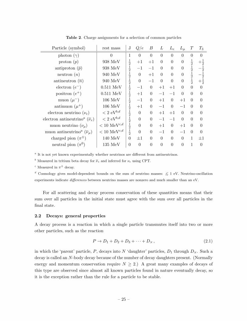
Table 2. Charge assignments for a selection of common particles

Particle (symbol) rest mass J Q/e B L Le Lµ T T3

photon (γ) 0 1 0 0 0 0 0 0 0

proton (p) 938 MeV 12 +1 +1 0 0 0 1

2 +12

antiproton (p) 938 MeV 12 −1 −1 0 0 0 1

2 −12

neutron (n) 940 MeV 12 0 +1 0 0 0 1

2 −12

antineutron (n) 940 MeV 12 0 −1 0 0 0 1

2 +12

electron (e−) 0.511 MeV 12 −1 0 +1 +1 0 0 0

positron (e+) 0.511 MeV 12 +1 0 −1 −1 0 0 0

muon (µ−) 106 MeV 12 −1 0 +1 0 +1 0 0

antimuon (µ+) 106 MeV 12 +1 0 −1 0 −1 0 0

electron neutrino (νe) < 2 eVb,d 12 0 0 +1 +1 0 0 0

electron antineutrinoa (νe) < 2 eVb,d 12 0 0 −1 −1 0 0 0

muon neutrino (νµ) < 10 MeVc,d 12 0 0 +1 0 +1 0 0

muon antineutrinoa (νµ) < 10 MeVc,d 12 0 0 −1 0 −1 0 0

charged pion (π±) 140 MeV 0 ±1 0 0 0 0 1 ±1

neutral pion (π0) 135 MeV 0 0 0 0 0 0 1 0

a It is not yet known experimentally whether neutrinos are different from antineutrinos.

b Measured in tritium beta decay for νe and inferred for νe using CPT.

c Measured in π± decay.

d Cosmology gives model-dependent bounds on the sum of neutrino masses: <∼ 1 eV. Neutrino-oscillation

experiments indicate differences between neutrino masses are nonzero and much smaller than an eV.

For all scattering and decay process conservation of these quantities means that their

sum over all particles in the initial state must agree with the sum over all particles in the

final state.

2.2 Decays: general properties

A decay process is a reaction in which a single particle transmutes itself into two or more

other particles, such as the reaction

P → D1 +D2 +D3 + · · ·+DN , (2.1)

in which the ‘parent’ particle, P , decays into N ‘daughter’ particles, D1 through DN . Such a

decay is called an N -body decay because of the number of decay daughters present. (Normally

energy and momentum conservation require N ≥ 2.) A great many examples of decays of

this type are observed since almost all known particles found in nature eventually decay, so

it is the exception rather than the rule for a particle to be stable.

– 25 –

Sometimes the decay in question can be understood because the parent is built from

smaller things and the decay represents either the decay of a constituent or the re-arrangement

or escape of some of the constituents. Most nuclear decays (the source of ordinary radioac-

tivity) turn out to be of this type:

• α Decays: correspond to the escape of a small He4 nucleus (i.e. an α-particle) from

a nucleus, and so always lower both Z and N by two (and so lower A by four): e.g.238

92U→ 23490Th+α is an example of a 2-body α-decay that is the start of the natural

Uranium radioactive chain.

• β Decays: usually10 correspond to the spontaneous decay of a neutron within the nu-

cleus, whose occurrence is no surprise given that free neutrons are also seen to decay.

The decay reaction for a free neutron is n → p+ + e− + νe, (where p or p+ denotes a

proton and e− denotes an electron while νe is a particle called an ‘electron anti-neutrino’

— more about this later). Since the decay takes a neutron to a proton it always in-

creases Z by one and leaves A unchanged, such as for the decay of radioactive Carbon:14

6C→ 147N+e−+ νe (which is the one used for carbon-14 radioactive dating). As we see

later, in these decays the outgoing electron (and neutrino) are created at the instant of

the decay and were not previously rattling around within the nucleus.

• γ Decays: correspond to the emission of a photon as the nuclear constituents fall from

an excited energy level to one at lower energies (like the ground state), and so do not

change Z or A at all. These are the nuclear analogs of the emission of light by atomic

transitions wherein an excited electron jumps down to a lower energy level. The main

difference is that nuclear γ transitions emit considerably more energy due to the larger

energy differences between nuclear energy levels compared with atomic energy levels.

Neutron decay is an example where the bound state involved in a decay is not a nucleus

but is instead something else. We shall see that neutrons (and more broadly all of the observed

particles that take part in the nuclear force — i.e. protons, neutrons and many other unstable

particles such as ‘pions’, π± or π0) are built from still-smaller constituents called quarks, and

some decays happen because of a decay of an underlying quark. For instance protons and

neutrons are built from two types of quarks, u and d, with a proton being a 3-quark bound

state uud while a neutron is a udd state, and neutron decay arises because of the decay of an

underlying quark: d→ u+ e− + νe.

Exercise: Use conservation of electric charge, baryon number and lepton number,

and the information that p is built as a uud bound state while n is a udd bound

state, to infer the charge, baryon number and lepton number of the u and d

10But not always: for some nuclei β decays can emit positrons — antiparticles to electrons — or sometimes

they instead absorb an atomic electron into the nucleus.

– 26 –

quarks. What do these assignments mean for the charge, baryon number and

lepton number assignments of the π± where π+ is a ud combination and π− is a

ud combination?

Not all decays involve the rearrangements or decays of constituents, however, since par-

ticles that appear to be elementary are also known to decay. So far as we know the decay

of a d quark is an example of this, as are other examples like the decay µ− → e− + νe + νµ

(where µ− — called a ‘muon’ — is an elementary particle that is 200 times heavier than

an electron, and νµ is a neutrino — called the ‘muon neutrino’ — that differs from the νe).

It is the appearance of two types of neutrino here that make this reaction consistent with

conservation of Le and Lµ, since Le(µ−) = 0 and Le(e

−) +Le(νe) +Le(νµ) = +1− 1 + 0 = 0

while Lµ(µ−) = +1 and Lµ(e−) + Lµ(νe) + Lµ(νµ) = 0 + 0 + 1 = +1.

Neutron decays are also instructive for another reason. If neutrons are unstable the

miracle is that any nuclei are stable at all, but (as we shall see) many are. Absolutely stable

nuclei are stable because the increased Coulomb energy associated with the new proton’s

electric charge can make the prospective daughter nucleus heavier than the putative parent

(and so the decay is forbidden by energy conservation). This observation teaches us (at least)

two things: first, it shows that even for unstable nuclei the actual nuclear β-decay rate is not

simply related to the decay rate of a free neutron. Nuclear decay rates range over many orders

of magnitude in size precisely because their computation often requires detailed knowledge of

the structure of the parent and daughter nucleus.

The stability of some nuclei — in spite of free-neutron decay — also shows that con-

servation laws can explain why some particles never decay. Energy conservation requires all

daughter particles to be lighter than their parent and so the lightest particle carrying a con-

served charge must be stable. So far as is known conservation laws are the reason why all

of the stable elementary particles do not decay. For instance, electrons are absolutely stable

because electric charge is conserved and there is no lighter particle carrying charge into which

the electron can decay. Similarly, protons would be absolutely stable if baryon number, B, is

conserved, but because we do not know whether B is exactly conserved there are doubts as

to whether or not the proton is exactly stable. (Even if unstable its decay lifetime is known

to be much longer than the age of the universe, so any failure in B conservation must be

extremely small.)

2.2.1 Decay Kinematics

Conservation laws strongly restrict the properties of decays, and sometimes control whether

or not a decay takes place at all. For instance for neutron decay, n → p + e− + νe, electric

charge balances because a neutron is electrically neutral and so the initial total charge is

Qi = Q(n) = 0. For the decay products the proton and electron have opposite charge and

the antineutrino is neutral, so Qf = Q(p) +Q(e−) +Q(νe) = +e− e+ 0 = 0. Baryon number

– 27 –

also balances because Bi = Bf = +1 with Bi = B(n) carried by the decaying neutron while

Bf = B(p)+B(e−)+B(νe) = +1+0+0 is carried purely by the final proton. Lepton number

is balanced because the initial neutron has Li = L(n) = 0 while the final lepton number is

Lf = L(p) + L(e−) + L(νe) = 0 + 1 − 1 = 0. Lepton number would not be conserved if the

antineutrino had instead been a neutrino, or if it carried L = 0.

Energy and momentum conservation similarly relate the initial and final states, with

EP =

N∑a=1

Ea and pP =

N∑a=1

pa , (2.2)

where Ea and pa are the energy and momentum of particle Da. Because each particle sat-

isfies E =√

p2 +m2, where m is that particle’s rest mass, and because the energy and the

momentum of the initial particle can be chosen when setting up the experiment, there are a

total of 3N unknowns (the components of the N final momenta) one would wish to deter-

mine. These unknowns are subject to the 4 constraints given in (2.2), and so in general we

expect there to be 3N − 4 free components of momentum that are not determined purely

from energy-momentum conservation.

This counting is particularly simple in the rest-frame of the decaying particle, for which

pP = 0 and so EP = mP . Consider first a two-body decay, P → D1 + D2, for which N = 2

and so only 3N − 4 = 2 of the 6 components of p1 and p2 are undetermined by energy-

momentum conservation. In this case because pP = 0 momentum conservation requires the

final momenta must sum to zero:

p1 + p2 = 0 , (2.3)

so the two daughter particles emerge back-to-back in the decaying particle rest frame. This

implies, in particular, that the magnitudes of their momenta are equal, and so therefore the

energies of the two final particles in this frame must be related by

E21 −m2

1 = E22 −m2

2 . (2.4)

But energy conservation also implies the energies in this frame must satisfy

E1 + E2 = mP , (2.5)

which only has solutions (for nonzero real momenta) if m1 +m2 < mP . These two equations

can be solved to determine the energies of both particles completely, giving:

E1 =m2P +m2

1 −m22

2mP

and E2 =m2P +m2

2 −m21

2mP

. (2.6)

In particular, E1 → E2 → 12 mP in the limit m1 +m2 mP .

Crucially: for two-body decays the energy of each of the decay products is completely

determined by energy-momentum conservation. All that the details of the physics responsible

– 28 –

for the decay can do is predict the likelihood for one of the particles to come out in a particular

direction. (Even this is not possible if the initial parent particle is rotation invariant — i.e

has no spin — since then all directions are equally likely.)

The same is not true when there are three or more particles in the final state. In this

case momentum conservation in the decay rest frame implies

p1 + p2 + p3 = 0 , (2.7)

which can be used to determine the momentum of one of the daughters in terms of the other

two. But this does not fix the magnitude of each of the particle momenta separately, so energy

can be shared between the other two particles consistently with overall energy conservation,

which in the decay rest-frame states

E1 + E2 + E3 = mP . (2.8)

Unlike for two-body decays, for three-body (or more-body) decays energy-momentum con-

servation is consistent with daughter particles emerging with a distribution of energies. For

instance, in nuclear β-decay the electron is seen to emerge from the decay with a distribution

of energies, as in Fig. 7, rather than a unique energy, and this is historically the way that the

existence of the antineutrino was initially inferred.

Figure 7. The distribution of electron energies obtained from the β decay of a nucleus. Because more

than one energy is possible we know β decay cannot be 2-body and so must involve at least three

particles in the final state. (Figure source: http://www.ohio.edu/people/piccard/radnotes/alphabeta.html).

2.2.2 Decay rates

The rest-frame decay probability per unit time (or decay rate), Γ, for a given particle is a

characteristic of that particle as intrinsic to it as is its mass or spin. The value of Γ depends

on the details of the interactions responsible for the decay, and because of this measurements

of Γ can be informative about these interactions.

Because the decay of any one particle is a random event decay measurements involve sta-

tistical properties of a collection of identical decaying individuals, so we need the probability

– 29 –

distribution, P(t), for a particle’s continued survival at time t, given its existence at an initial

time t0. Now Γ is time-independent and Γ dt gives the probability for decay to occur in any

given short time window, dt, so the probability of there not being a decay in this interval is

1−Γ dt. Consequently the survival probability, P(t+ dt) = P(t) + dP, at time t+ dt is given

in terms of the survival probability, P(t), at t by

P(t) + dP = P(t) (1− Γ dt) and so dP = −ΓP(t) dt , (2.9)

where the factor P(t) after the first equality is the probability of surviving to time t, while

the second factor is the probability of also surviving the next interval dt.

The result dP/dt = −ΓP integrates to give an exponential distribution

P(t) = Γ e−Γ(t−t0) , (2.10)

with an integration constant chosen to normalize the result on the interval t0 ≤ t <∞. This

shows that one way to measure Γ is by measuring the mean life, τ , of the decaying particles

to survive (given their presence at the initial time t0), defined by

τ :=

∫ ∞t0

dt (t− t0)P(t) =1

Γ. (2.11)

Another way to get at the same quantity is by counting the population of undecayed

particles in a sample as a function of time. For a collection of n0 particles at time t0 the

number of surviving particles at a later time t is n(t) ∝ P(t), and so

n(t) = n0 e−Γ(t−t0) . (2.12)

Another measure of Γ is then the half-life, τ1/2, defined as the time taken for half of a given

sample to decay (a result which doesn’t depend on the size of the initial sample for exponential

decays):

n(t− t0 = τ1/2) =n0

2=⇒ τ1/2 =

ln 2

Γ' 0.693 τ . (2.13)

The decay rate of a moving particle differs from the rest-frame rate because of time

dilation. In a reference frame for which the decaying particle has speed v = p/E the mean

decay life is longer by the Lorentz transformation formula

τ(E) = γ τ =τ√

1− v2=Eτ

mand so Γ(E) =

mΓ

E. (2.14)

Time-dilation of decay lifetimes is a well-established experimental fact. For example,

muons were initially discovered once radiation detectors were developed because we are con-

stantly bombarded (several per square metre per second at the Earth’s surface) by energetic

muons coming down from the top of the atmosphere. Muons are produced there as byprod-

ucts of nuclear reactions when cosmic rays — i.e. mostly energetic protons — hitting the

– 30 –

Earth from space collide with atomic nuclei in the upper atmosphere. But muons produced

in the lab are seen to decay with lifetimes of about a microsecond, and at face value this

causes a problem since even if moving at the speed of light a particle can move only 300

m in a microsecond. The problem is that the top of the atmosphere (where the muons are

produced) is many kilometres up and so how can the muons live long enough to get down to

the Earth’s surface to be discovered? The resolution is time dilaton: although muons decay

in microseconds in their rest frame, they are sufficiently energetic that they live long enough

to an observer at rest on the Earth to survive the trip through the atmosphere.

2.2.3 Line widths

The above methods for measuring Γ are fine if the decay is slow enough. Nuclear decays are

seen with an enormous range of half-lives — running from lifetimes in the billions of years

down to lifetimes measured in small fractions of a second — so for many the above methods

suffice. But many other decays are much faster: examples discussed in later sections can have

Γ ' 1 GeV, and so τ = 1/Γ ' 1 GeV−1 ' 6× 10−25 s, and even moving at the speed of light

a particle decaying this fast could only traverse about 0.2 fm – i.e. much less than the size

of a nucleus. Decays this fast happen so quickly that the parent particle is not directly seen.

How is Γ measured when this is so?

For decays this rapid we must zoom out a bit and consider the reaction that produced

the decaying particle in the first place. For concreteness, suppose the decaying particle, P , is

produced as an intermediate state in a 2-body reaction, A+B → C+D, in which particles A

and B are collided and are converted into particles C and D that are long-lived and so can be

observed leaving the scene. We imagine that for at least some of these reactions this process

occurs in two steps: A+B → P after which P decays through the process P → C+D. (Such

a two-step process is called a resonant channel.) We also allow that there may be several

other reaction channels leading from A+ B to C +D that do not require the creation of an

intermediate P particle, which we call ‘prompt’ since they are usually faster (not needing to

wait for P to decay). We imagine preparing the initial particles with specific energies, EA

and EB, and measuring the final energies, EC and ED, (and sometimes also the directions)

of the outgoing particles, and the goal is to identify whether the two-step decay reaction

A + B → P → C + D can be distinguished from any prompt reactions even if the decay is

much too fast for the lifetime to be directly measured. And if they can be distinguished we

wish to see how to infer the value of Γ for the decay.

Although the details are not important for what follows, there are a variety of specific

reactions of this form that are of practical interest. One such is the reaction e+e− → e+e−

or the reaction e+e− → µ+µ−, which proceed both through the electromagnetic and the

weak interactions. These reactions (and others) were studied in detail using electron-positron

colliders, culminating with the Large Electron-Positron Collider (LEP, at CERN in Geneva)

and the Stanford Linear Collider (SLC, in California) in the late 1980s and early 1990s. These

– 31 –

experiments were the first to have sufficient energy to produce a Z boson (whose mass is 90

GeV) and for energies around 90 GeV the ‘decay’ version of the reaction takes place by first

having e+e− → Z, with the produced Z then decaying to the final state, Z → e+e− or

Z → µ+µ−. A plot of measurements for a similar reaction (e+e− → qq, where q means any

species of quark – a particle from which strongly-interacting particles turn out to be built) is

given in Figure 8. The ‘prompt’ version of these reactions are understood as arising due to

the exchange of photons and W bosons, but never through their direct production and decay.

The resonant-decay channel only occurs11 (for this choice of initial particles) for the Z.

Figure 8. The Z boson resonance in the cross section for e+e− → hadrons (strongly interacting

particles). The black line is the theoretical prediction of the Standard Model while the coloured points

are measurements made at various accelerators. The large resonance peak occurs at the Z-boson mass,

MZ ' 90 GeV and its width characterizes the Z boson lifetime as described in the main text. (Figure

source: http://tlep.web.cern.ch/content/what-are-line-shape-parameters-resonance).

Since the prompt and decay mechanisms are independent of one another but share the

same initial and final state their amplitudes must be summed:

Atot(AB → CD) =

∫ ∞−∞

dt0

[Apr(t0) +Adc(t0)

], (2.15)

where subscripts ‘pr’ and ‘dc’ denote the prompt and decay contributions, and there is an in-

tegration over the unknown time, t0, when the reaction takes place. The reaction probabilities

are then the squares of the amplitude, P = |A|2 (as usual in quantum mechanics).

11It turns out there are other states besides the Z that can be produced and then decay, but these consist

of quark-antiquark bound states and do not contribute much at these energies, for reasons that will become

clear shortly.

– 32 –

For the decay contribution the amplitude comes with an additional sum over the time

between production of P and its decay, since we do not know precisely when the decay occurs:

Adc(t0) =

∫ ∞t0

dtA(AB → P ; t0)A(P ; t− t0)A(P → CD; t) , (2.16)

where A(AB → P ; t0) is the amplitude for producing the intermediate state, P , at time t0,

A(P ; t− t0) is the amplitude for the P state to survive from t0 until t ≥ t0 and A(P → CD; t)

is the amplitude for the decay P → C +D at time t. It is the delay t− t0 caused by waiting

for P to decay that allows us to distinguish the prompt from the decay reaction.

The important point is that the t- and t0-dependence of these amplitudes is fairly simple

to track. It arises in two ways: one is the contribution from the wave-function for each of the

particles involved, ψa ∝ e−iEat, and since the amplitude is an inner product, A ∼ ψ∗f ψi, this

becomes ψ∗a ∝ e+iEat for any particle in the final state:

Apr(t0) = AAB|CD e−i(EA+EB−EC−ED)t0

A(AB → P ; t0) = AAB|P e−i(EA+EB−EP )t0 (2.17)

and A(P → CD; t) = AP |CD e−i(EP−EC−ED)t .

The other source of t dependence is the exponential decay survival probability for P as it

awaits its decay. That is,

A(P ; t− t0) = iAP e−Γ(t−t0)/2 , (2.18)

where AP is independent of time, and the factor of i is purely conventional. This last equation

is required to allow the modulus of ψP (t) to shrink exponentially, as it must since the survival

probability is the square of the amplitude, P(P ; t − t0) ∝ |A(P ; t − t0)|2 ∝ e−Γ(t−t0), as

required by the exponential decay law described above.

Consequently, the t- and t0-dependence of the decay contribution to the integrand in

(2.16) is

AAB|PAP |CDAP e−i(EA+EB−EC−ED)t0 e−i[(EP−iΓ/2)−EC−ED](t−t0) , (2.19)

and this must be added to Apr, whose t0-dependence is given in (2.17). The t-integration is

then elementary, and once this is done both prompt and decay terms share the common factor

e−i(EA+EB−EC−ED)t0 , whose integration with respect to t0 gives the usual energy-conserving

delta-function: 2π δ(EA+EB−EC−ED). The total amplitude found by summing the prompt

and decay processes then becomes

Atot(AB → CD) = 2π

[AAB|CD +

AAB|PAP |CDAP(EP − Etot)− iΓ/2

]δ(EA + EB − EC − ED) , (2.20)

where Etot = EA + EB is the total energy available in the initial state.

Now comes the main point. The coefficients AAB|CD and AAB|P etc can depend on Etot,

but this dependence is usually not particularly strong in the immediate vicinity of Etot = EP .

– 33 –

Consequently, if Γ EP (a condition called the narrow-resonance condition), then it is the

denominator in the second term of the square bracket that dominates the Etot-dependence of

the rate very near Etot = EP . Since its square has the form∣∣∣∣ 1

(EP − Etot)− iΓ/2

∣∣∣∣2 =1

(Etot − EP )2 + (Γ/2)2, (2.21)

this gives a large enhancement or resonance to the reaction rate, regarded as a function of

Etot, occurring precisely at EP . The Etot-dependence predicted in (2.21) is universal and is

called the Breit-Wigner (or, in the relativistic context, Lorentzian) line-shape.

Whenever this characteristic line-shape is observed, the width Γ is easily determined

from the width of the resonant peak, given for example by its full width at the place where

the resonance has fallen off to half of its maximum value (i.e. the peak’s ‘full-width half-

max’). For example, Fig. 8 plots the predicted and measured reaction rate for the reaction

e+e− → hadrons (essentially quarks), which shows precisely this shape near the Z boson

mass. Sometimes new particles are discovered by performing a ‘bump hunt’ that search for

resonances whose presence could indicate the existence of something hitherto undiscovered.

The most recent example of such a discovery is the Higgs boson, whose decay into two photons

was discovered through the presence of an unexpected bump in the photon production rate

at the Large Hadron Collider (LHC) at CERN. Figure 9 shows the Higgs bump due to the

decay H → γγ.

2.2.4 Differential decay rates

Decays into multiple daughters can sometimes give additional information, through the angu-

lar distribution of the decay products. This information is contained within the differential de-

cay rate, which can be informative about the spin of the decaying particle and about the nature

of the underlying interactions that are in play. The differential decay rate, dΓ/d3p1 · · · d3pN ,

regarded as a function of p1 through pN , is the joint probability per unit time for a decay

process with particle D1 emitted within a small volume d3p1 of p1, particle D2 emitted within

a volume d3p2 about p2 and so on up to particle DN having momentum within the volume

d3pN of pN . In terms of this the total decay rate discussed above is given by

Γ =

∫d3p1 · · · d3pN

(dΓ

d3p1 · · · d3pN

). (2.22)

It is useful to define the differential decay rate in a way that is Lorentz invariant, since

then it can be computed once and for all with the result useful for decays of particles in any

reference frame. For the decay P → D1(p1)+D2(p2)+ · · ·+DN(pN) the invariant differential

decay distribution, M(pP ; p1, · · · pN), is related to the above differential decay rate by

dΓ

d3p1 · · · d3pN=

1

2EP

[M(pP ; p1, · · · ,pN)

[(2π)32E1] · · · [(2π)32EN ]

](2π)4δ4(pP − p1 − p2 · · · − pN) , (2.23)

– 34 –

Figure 9. The Higgs boson resonance in the cross section for producing two photons in the CMS

detector at the Large Hadron Collider. The top curve shows both prompt events and Higgs de-

cays while the bottom panel is after the prompt events have been subtracted out. (Figure source:

http://cms-results.web.cern.ch/cms-results/public-results/publications/HIG-14-016/index.html).

where the delta-function sets the sum of final 4-momenta, pµ1 + · · ·+ pµN , equal to the initial

4-momentum, pµP , so (in the centre-of-mass frame)

δ4(pP − p1 − · · · pN) := δ(EP − E1 − E2 · · · − EN) δ3(p1 + · · ·+ pN) . (2.24)

The Lorentz-invariance of M relies on the observation that Γ transforms as does m/EP

and so the rest must be invariant. Furthermore, the 4-dimensional delta-function is invariant

since it imposes a relation amongst 4-momenta that all transform in the same way, and the

measure d3p/E for each particle is also Lorentz-invariant, as can be seen by directly following

through the transformations that take p and E to p′ and E′.

Exercise: Derive the transformation law for E and p (as a function of coshβ and

sinhβ) for a boost along the z axis from the transformation law of the energy-

momentum 4-vector, (p′)µ = Λµν pν . By directly using these prove that dpx, dpy

and dpz/E are invariant (from which we learn d3p/2E is also invariant, as claimed

in the text).

Alternatively, the invariance of d3p/E can be seen by starting from the manifestly in-

– 35 –

variant starting point∫d4p δ(pµp

µ +m2)ϑ(p0)(· · · ) =

∫d3p dp0 δ

[−(p0)2 + E2

]ϑ(p0)(· · · ) =

∫d3p

2E(· · · )|p0=E ,

(2.25)

where pµpµ := ηµν p

µpν so the delta-function imposes the condition (p0)2 = E2 where E :=√p2 +m2 and the step-function, ϑ(x) = 0 if x < 0 and 1 if x > 0, tells us to take the

positive root when doing so. This condition on the sign of p0 is also Lorentz-invariant because

the delta-function tells us that pµ is time-like (and so all observers agree on the sign of p0).

Finally, the factor of 2E in the denominator of (2.25) arises from the change-of-variable

formula for the Dirac delta-function, about which we pause to amplify because it is also useful

later. Recall that δ(x − y) is defined to vanish for x 6= y (and diverge for x = y) in such a

way that ∫dy δ(x− y)f(y) = f(x) (2.26)

for any integration region including y = x and any sufficiently smooth function f . But the

delta function in (2.25) instead comes in the form12∫

dy δ[g(x, y)] f(y) and so its evaluation

requires a few extra steps:∫dy δ[g(x, y)] f(y) =

∫dg

|∂g/∂y|δ(g) f(y) =

(f(y)

|∂g/∂y|

)y=y(x)

, (2.27)

where the first equality changes the integration variable to agree with the argument of the

δ-function (so as to use (2.26)), and y = y(x) is the (assumed unique within the integration

region) solution to g(x, y) = 0.

It is the invariant quantityM that we later relate to the square of a scattering amplitude

once we try to compute the decay rate starting from an underlying theory of the interactions.

Once this is done we will find

M =⟨|A|2

⟩, (2.28)

where A is an invariant amplitude (often the matrix element of some interaction Hamiltonian,

A = 〈f |Hint|i〉, between an initial state, |i〉, and a final state, |f〉) and 〈· · · 〉 denotes a sum

over unmeasured quantum numbers (such as spin) in the final state, and an average over

unmeasured quantum numbers in the initial state.

With these definitions, once the invariant quantityM is known, the total rate is computed

using

dΓ(P → F ) =1

2EP

M (2π)4δ4(pP − pF ) dβF , (2.29)

where F = D1 + · · ·+DN here collectively denotes all of the final daughter particles, and so

pF is short-hand for the sum over final-state 4-momenta: pµF = pµ1 + · · ·+ pµN . Finally, the last

12Explicitly, in the example of interest y = p0, x = E and g(x, y) = x2 − y2 so g = 0 implies y = ±x and

|∂g/∂y| = 2y.

– 36 –

factor denotes the combination

dβF :=d3p1

(2π)32E1· · · d3pN

(2π)32EN

. (2.30)

The total rate is obtained by integrating over all possible final-state momenta, and because

this volume of integration is called the reaction’s phase space, the product in (2.30) is called

the Lorentz-invariant phase-space (or LIPS) measure.

Exercise: Evaluate the integrals over Lorentz-invariant phase space and show

that for two-body decay the differential decay rate for emission of one of the

daughters into an element of solid angle, dΩ, is given in the rest frame of the

decaying particle by

dΓ

dΩ(A→ B + C) =

M p

32π2m2A

(decay rest frame) , (2.31)

where p =√E2C −m2

C =√E2D −m2

D is the magnitude of the momentum of either

of the daughter particles. Given the daughter energies are EB = (m2A + m2

B −m2C)/2mA and EC = (m2

A +m2C −m2

B)/2mA show that this means

p =

√[m2

A − (mB +mC)2][m2A − (mB −mC)2]

2mA

. (2.32)

Exercise: The charged pion, π+, decays almost always into µ+νµ. It turns out

the invariant matrix element for this decay is

M(π+ → µ+νµ

)= 2mπp

(2GF |Vud|mµFπ

)2, (2.33)

where p is the magnitude of the neutrino momentum in the decay rest frame,

mπ = 140 MeV is the charged pion mass, mµ = 105 MeV is the muon mass and

GF = 1.166379 × 10−5 GeV−2 is Fermi’s constant and |Vud| = 0.974 is called a

Kobayashi-Maskawa matrix element. The quantity Fπ is the pion decay constant,

whose value is determined by the comparing this decay rate with the measured

lifetime (once GF is determined from µ+ decay and |Vud| from nuclear β decay).

Compute the total decay lifetime of the pion and show that it is given by

Γ(π+ → µ+νµ) =G2F |Vud|2m2

µmπF2π

4π

(1−

m2µ

m2π

)2

. (2.34)

Compare this to the measured mean life (2.6033± 0.0005× 10−8 sec), to see what

the experimental value is for Fπ. π+ → e+νe can also occur, and does so with a

– 37 –

rate obtained from the above by substituting mµ → me (where me = 0.511 MeV).

What is the ratio Rπ = Γ(π+ → e+νe)/Γ(π+ → µ+νµ) numerically? Naively this

ratio is something of a puzzle since electrons and muons participate in interactions

with the same strength and the electron provides more phase space into which to

decay, so one might have expected Rπ 1. The fact that this is not true tells us

about the spin-dependence of the underlying weak interactions.

Exercise: The neutral pion, π0, decays almost always into two photons. It turns

out the invariant matrix element for this decay is

M(π0 → γγ

)= 2

[αm2

π

2πFπ

(Nc

3

)]2

, (2.35)

where mπ = 135 MeV is the neutral pion mass and α = 1/137 is the fine-structure

constant. The quantity Fπ = 92 MeV is called the pion decay constant, and can

be measured in the decay process π+ → µ+νµ. Finally, Nc is the number of

colours carried by each quark inside the pion (more about which later). Compute

the total decay rate of the pion and show it is

Γ(π0 → γγ

)=

α2m3π

(4π)3F 2π

(Nc

3

)2

. (2.36)

(Careful: the two photons are completely indistinguishable. What is the proper

solid angle through which one should integrate dΓ/dΩ if we are not to double-

count?) Evaluate this and compare the result to the measured mean life (8.52±0.18× 10−17 sec), to see what the experimental value is for the number of quark

colours.

2.3 Scattering: general properties

The other major source of information about subatomic particles comes from studying col-

lisions wherein the bringing together of several (in subatomic physics usually two) particles

initiates a reaction of some sort, such as

A+B → F1 + F2 + · · ·FN , (2.37)

which is a 2 → N collision corresponding to having two particles collide with N particles

leaving the reaction. Elastic collisions form the important special case of a 2 → 2 collision

for which the final two particles are identical to the initial two: A + B → A + B. All other

collisions are called inelastic, because some of the initial kinetic energy has been converted

into changing particle types. We next review the convenient ways to characterize the reaction

rates for such collisions.

– 38 –

2.3.1 Cross sections and luminosity

Very rarely do experiments in subatomic physics prepare particles only one at a time for

collisions, since normally a collection of particles are first accelerated to some energy in

a high-energy beam before being brought to collide, either with another beam or with a

stationary fixed target. Usually the more particles in the beam and target the more collisions

there will be.

When particles collide there are two kinds of things that determine the reaction rate.

Some of these are fairly mundane, like the number of particles involved (more particles means

more potential reactions) and their speeds and other adjustable properties as they collide.

Others are more fundamental, such as the interactions the particles experience. The goal

of this section is to express the reaction rate for a collision in terms of an initial luminosity

(which captures the mundane features specific to the particular way the particles were brought

together) and an interaction cross section that contains the information about the interactions

involved.

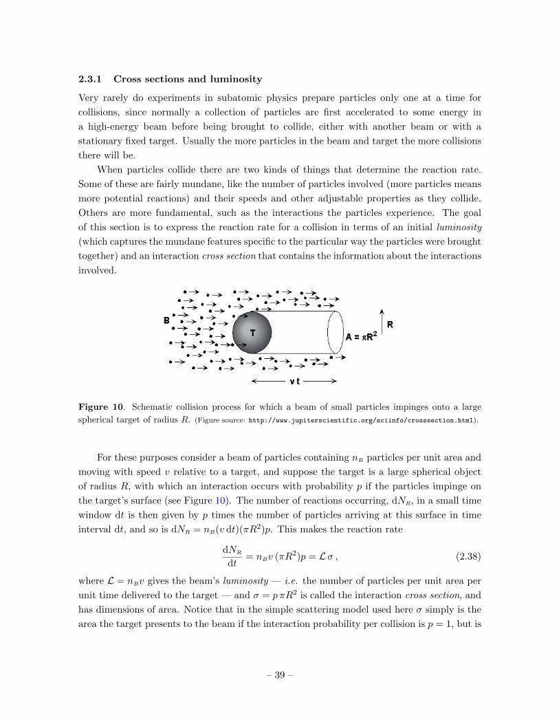
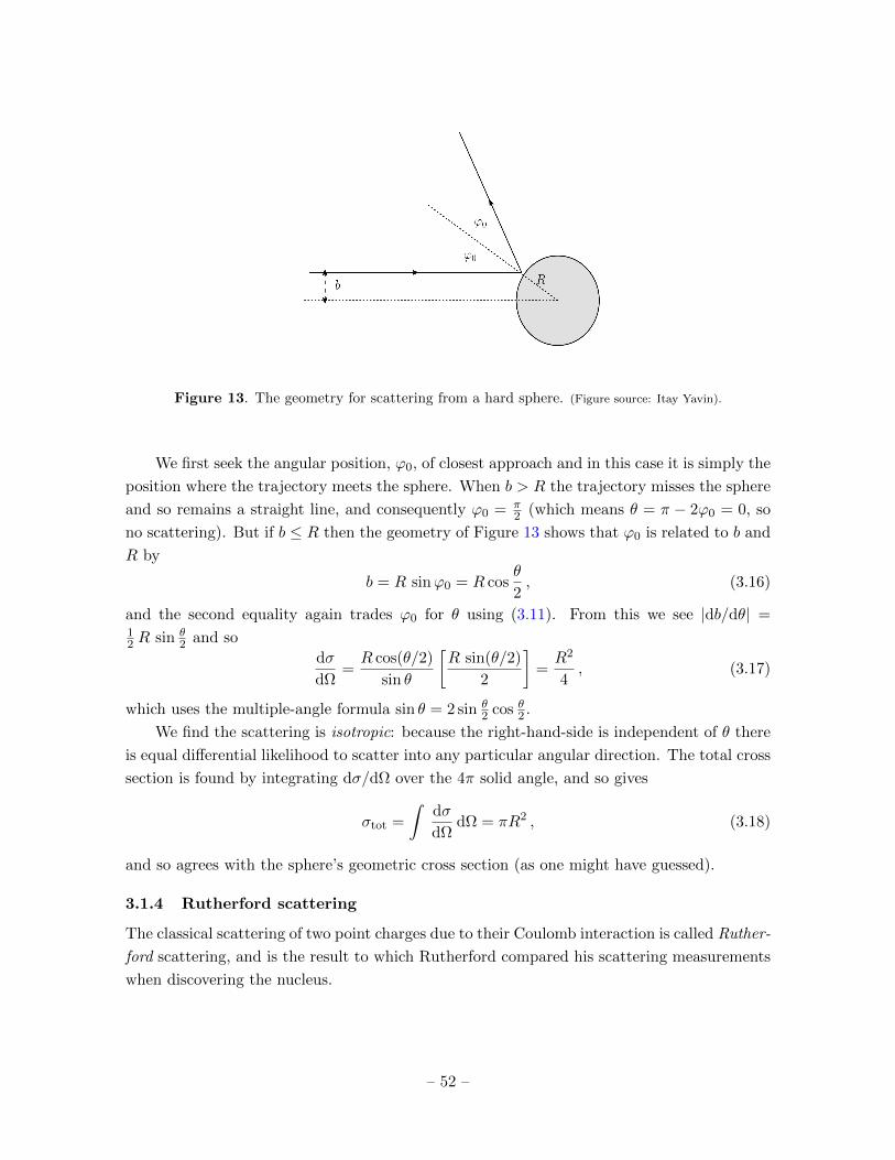
Figure 10. Schematic collision process for which a beam of small particles impinges onto a large

spherical target of radius R. (Figure source: http://www.jupiterscientific.org/sciinfo/crosssection.html).

For these purposes consider a beam of particles containing nB particles per unit area and

moving with speed v relative to a target, and suppose the target is a large spherical object

of radius R, with which an interaction occurs with probability p if the particles impinge on

the target’s surface (see Figure 10). The number of reactions occurring, dNR, in a small time

window dt is then given by p times the number of particles arriving at this surface in time

interval dt, and so is dNR = nB(v dt)(πR2)p. This makes the reaction rate

dNR

dt= nBv (πR2)p = Lσ , (2.38)

where L = nBv gives the beam’s luminosity — i.e. the number of particles per unit area per

unit time delivered to the target — and σ = p πR2 is called the interaction cross section, and

has dimensions of area. Notice that in the simple scattering model used here σ simply is the

area the target presents to the beam if the interaction probability per collision is p = 1, but is

– 39 –

smaller otherwise. More generally (such as if target and beam interact at a distance through

long-range forces, or once diffractive quantum wave behaviour is considered) it is possible

also to have σ be larger than the target’s cross-sectional area.

Instantaneous luminosity is a property of the accelerator that produces the beam, and a

typical example from a modern accelerator might be of order L = 1034 cm−2 s−1. Integrated

luminosity, L, is another useful statistic that gives the total number of particles per unit area

delivered on target over some time window (such as the lifetime of an experiment, say),

L(T ) =

∫ t0+T

t0

dt L(t) , (2.39)

which has units of inverse area. For instance, delivering the above luminosity for T = 1 year

' 3×107 s gives an integrated luminosity L ' 3×1041 per square cm. Multiplying integrated

luminosity times cross section, N = σL, directly gives the total number of scattering events

that occur over the given time window, T .

Of course we would be nuts to continue using CGS (or SI) units here, and for subatomic

physics something closer to the dimensions of a nucleus makes a better reference unit. The

conventional choice is the barn (or b) defined as

1 b = 10−24 cm2 = 10−28 m2 = (10 fm)2 . (2.40)

The usual metric prefixes apply, so 1 mb (or millibarn) is 10−27 cm2, 1 µb (or microbarn)

is 10−30 cm2, 1 nb (or nanobarn) is 10−33 cm2, 1 pb (or picobarn) is 10−36 cm2 and 1 fb

(or femtobarn) is 10−39 cm2, and so on. These units are also useful for describing integrated

luminosity, with L = 1 pb−1 corresponding to 1036/cm2. In these units L ' 3 × 1041 cm−2

becomes L ' 100 inverse femtobarns, and so even cross sections as small as σ ' 1 fb would

generate 100 events given this much integrated luminosity.

2.3.2 Invariant and differential cross section

One drawback of the previous section is that it is entirely phrased within the rest-frame of

the target, and so the separation of the rate into a luminosity piece and a cross-section piece

is not yet Lorentz invariant. This is a drawback because not all experiments are done with

motionless targets (an example is a colliding beam experiment — like the LHC or LEP —

which collide two beams into one another head on). This section aims in part to correct this

drawback.

Furthermore, we are usually interested not just in the total cross section but also in the

differential cross section, for which specific values of final-state momenta are specified for the

outgoing particles. It is also useful to define this in a Lorentz-invariant way, making it easier

to convert predictions to any particular frame of interest for a specific experiment.

– 40 –

The starting point for defining things covariantly is the reaction rate, Γ, and its differential

counterpart

Γ(AB → F1 · · ·FN) =

∫d3p1 · · · d3pN

(dΓ

d3p1 · · · d3pN

). (2.41)

For a two-particle initial state Γ transforms under Lorentz transformations like 1/(EAEB) —

one way to see this is because the process AB → F1 · · ·FN could have been the independent

decay of the initial particles A and B rather than a collision, and we have seen above that

each decay rate separately transforms like 1/E for the particle decaying. Keeping in mind, as

before, that the measure d3p/E is Lorentz-invariant suggests defining the invariant scattering

rate, M(pA,pB; p1, · · · ,pN), by

dΓ

d3p1 · · · d3pN=

nB2EA2EB

[M(pA,pB; p1, · · · ,pN)

[(2π)32E1] · · · [(2π)32EN ]

](2π)4δ4(pA + pB − p1 − p2 · · · − pN) ,

(2.42)

where, as before, nB denotes the density of beam particles and the delta-function sets the

sum of final 4-momenta, pµ1 + · · ·+ pµN , equal to the initial 4-momentum, pµA + pµB. It is again

M = 〈|A2|〉 that is related to squares of scattering amplitudes computed using an underlying

theory.

We can now use M to perform the split into luminosity and cross section in a way that

makes the cross section also a Lorentz-invariant quantity. We do so by writing

dσ =dΓ

F(2.43)

as before, but now where F is chosen to: (i) agree with L = nBvrel when the target (particle,

A, say) is at rest; and (ii) transform as does Γ to ensure dσ is Lorentz-invariant. Here vrel —

defined as the relative speed of the incident beam particles relative to the target — is itself a

Lorentz-invariant quantity, given in terms of the invariant dot product, pA ·pB = ηµνpµAp

νB ≤ 0,

of initial 4-momenta by

vrel =

√1− m2

Am2B

(pA · pB)2. (2.44)

Exercise: Prove the above relation for vrel by evaluating the quantity pA · pB in

terms of vrel in the rest-frame of one of the particles, and then solving for vrel.

The solution to condition (ii) is F = nBf/(2EA2EB) where f is any Lorentz-invariant

quantity (and the factors of 2 are conventional). Condition (i) then tells us

f = −4vrel(pA · pB) = 4√

(pA · pB)2 −m2Am

2B , (2.45)

because then F → nBvrel when pA → 0.

– 41 –

There are two particularly useful frames of reference in 2→ N scattering processes. One,

usually called the lab frame, is the frame13 in which one of the initial particles at rest. This

is the frame within which our original discussion of luminosity and cross section was done.

In the lab frame (rest-frame of B) and the c.o.m. frame f becomes

f = 4mBEAvrel = 4mBpA lab (lab frame)

and f = 4√

(EAEB + p2A)2 −m2

Am2B = 4(EA + EB)cm pA cm (c.o.m. frame) . (2.46)

The final expression for the invariant differential cross section then is

dσ(I → F ) =Mf

(2π)4δ4(pI − pF ) dβF , (2.47)

where I = A+ B denotes the initial 2-body state and pµI = pµA + pµB denotes the total initial

4-momentum, while (as before) F = F1 + · · ·FN denotes all of the final-state particles and so

pµF = pµ1 + · · ·+ pµN . The Lorentz-invariant phase space measure, dβF , is given by (2.30).

2.3.3 2→ 2 cross section

To make this more concrete let’s work out dσ(AB → CD) more explicitly for the special case

of 2→ 2 scattering. In this case there are two particles in the final state, and so

dσ(AB → CD) =Mf

(2π)4δ4(pA + pB − pC − pD) dβF (2.48)

=Mf

(2π)4δ(EA + EB − EC − ED) δ3(pA + pB − pC − pD)d3pC

(2π)32EC

d3pD(2π)32ED

.

As stated earlier, the four conditions given by energy-momentum conservation have removed

four of the six independent components of final momenta, and so for a 2-body final state we

can take the two quantities undetermined by conservation laws to be the angles specifying

the direction of the momentum of one of the outgoing particles: particle C, say.

We now perform the integral over the delta functions explicitly. We start with the integral

over one of the two final momenta, say pD, whose integration with the momentum-conserving

delta function amounts to everywhere replacing pD with pA + pB − pC . Next write out the

d3pC integral in polar coordinates using d3p = dpxdpydpz = p2dpdΩ where p = |p| and the

differential element of solid angle is dΩ = sin θ dθdφ with (θ, φ) giving the direction of p, as in

Figure 11. The energy-conserving delta function then allows us also to perform the integral

over |pC | as well, leaving only the angular integrals undone. When doing the |pC | integral

13The lab frame is indeed the reference frame of the laboratory in ‘fixed-target’ experiments in which a

beam is collided with a stationary target. The lab frame need not be the rest frame of the physical laboratory,

however, in collider experiments for which collisions occur between a pair of incident beams.

– 42 –

Figure 11. Definition of the angles θ and φ for the outgoing momentum pC . (Figure source:

https://commons.wikimedia.org/wiki/Spherical polar coordinates.png).

care must be used to properly use (2.27) for changing variables with the δ-function, leading

to the result

(2π)4 δ4(pI − pF ) dβF = (2π)4 δ4(pA + pB − pC − pD)d3pC

(2π)32EC

d3pD(2π)32ED

= 2π δ(EA + EB − EC − ED)d3pC

(2π)34ECED

∣∣∣∣pD=pA+pB−pC

(2.49)

=p2C dΩC

(2π)24ECED|d(EC + ED)/dpC |

∣∣∣∣pD=pA+pB−pC , EC=EA+EB−ED

=p3C dΩC

(4π)2|(EDpC − EC(pA + pB)) · pC |

∣∣∣∣pD=pA+pB−pC , EC=EA+EB−ED

.

and so the differential cross section for 2→ 2 scattering is

dσ

dΩ(AB → CD) =

[M p3

C

(4π)2f |(EDpC − EC(pA + pB)) · pC |

]pD=pA+pB−pC , EC=EA+EB−ED

,

(2.50)

where the right-hand side is to be regarded as a function of the direction, (θ, φ), of the outgoing

momentum pC . The total cross section, σ, is then obtained by integrating this result over all

possible such directions.

2.3.4 Lab and centre-of-mass frames

In the lab frame we can take pB = 0 and EB = mB, and so

dσ

dΩ(AB → CD) =

[M p3

C

(4π)2f |(EDpC − ECpA) · pC |

]pD=pA−pC , EC=EA+mB−ED

(lab frame)

=

[M p2

C

(8π)2mBpA|EDpC − ECpA cos θ|

]pD=pA−pC , EC=EA+mB−ED

, (2.51)

– 43 –

which uses f = 4vrelmBEA = 4mBpA in the lab frame. In the special case where the incident

particle (and its scattered partner) is massless, EA = pA and EC = pC this becomes

dσ

dΩ(AB → CD) =

[MEC

(8π)2mBEA|ED − EA cos θ|

]pD=pA−pC , EC=EA+mB−ED

, (2.52)

For most purposes a much more convenient frame is the centre-of-mass frame (or c.o.m.

frame), defined by the condition that pI := pA + pB = 0. This frame is particularly simple

both because it implies |pA| = |pB| (and so also E2A−m2

A = E2B−m2

B), and also because with

momentum conservation it also implies pC + pD = 0 (and so E2C −m2

C = E2D −m2

D).

As an example of how things often simplify in the c.o.m. frame, consider expression

(2.50). In this frame we have (EDpC − ECpD) · pC = (ED + EC)pC · pC = EI p2C , where the

initial total energy is EI = EA + EB = EC + ED. As a result (2.50) simplifies to become

dσ

dΩ(AB → CD) =

[M pC

(4π)2f(EA + EB)

]pD=−pC , EC=EA+EB−ED

(2.53)

=

[M pC

(8π)2pA(EA + EB)2

]pD=−pC , EC=EA+EB−ED

(c.o.m. frame) ,

Because pA = −pB in the c.o.m. frame the initial momenta are parallel to one another,

and so we can choose the direction they define to be the z-axis. In this case the angles (θ, φ)

describe the direction of the line defined by the parallel final-state momenta relative to this

initial direction. With this choice shifting φ corresponds to rotating the collision about the

axis defined by the initial beam. It is often true that the physics is invariant under such a

rotation, and when this is so the cross section is independent of φ and so depends nontrivially

only on θ. In this case the angular integral over φ amounts to multiplication of the result by

2π, leaving

dσ

sin θCdθC(AB → CD) = 2π

(dσ

dΩ

)(AB → CD) (axially symmetric) (2.54)

=

[M pC

32π pA(EA + EB)2

]pD=−pC , EC=EA+EB−ED

(c.o.m. frame) .

When this is true then there is only one independent final-state variable, θ, on which cross

sections can nontrivially depend (in addition to their dependence on the choice of total initial

energy, Ecm = EA + EB).

2.3.5 2→ 2 relativistic variables

Although formulae like (2.50) and (2.53) have the virtue of explicitness, they obscure Lorentz

invariance and so make it more cumbersome to relate observables in different reference frames.

For this purpose an alternative set of explicitly Lorentz-invariant variables, called Mandelstam

variables, are often used instead of θ and φ to describe 2→ 2 scattering.

– 44 –

The Mandelstam variables are built directly in terms of the 4-momenta: pµA, pµB, pµC and

pµD, and start with the observation that any Lorentz-invariant function of momenta (such as

M, for instance) can always be written as a function of the invariant inner products of these

four 4-vectors: e.g. pA · pB = ηµν pµAp

νB. Because the inner product of a 4-momentum with

itself is always the corresponding particle mass, pA · pA = −m2A and so on, they are constants

and the only possible independent kinematic variables must be

pA · pB , pA · pC , pA · pD , pB · pC , pB · pD and pC · pD . (2.55)

Even these are not all independent because, for example, 4-momentum conservation

implies we can always eliminate pµD using pµA+pµB = pµC+pµD, leaving three possible independent

combinations like pA · pB, pA · pC and pB · pC . The conventional way to group these three

quantities is into the Mandelstam variables s, t and u defined by

s := −(pA + pB) · (pA + pB) = −2pA · pB +m2A +m2

B ,

t := −(pA − pC) · (pA − pC) = +2pA · pC +m2A +m2

C , (2.56)

and u := −(pA − pD) · (pA − pD) = +2pA · pD +m2A +m2

D .

But we know that energy-momentum conservation and axial symmetry should only allow

us two independent variables, the total initial energy and scattering angle in the c.o.m.,

for example. So we expect that even these three quantities, s, t and u, cannot really be

independent. This expectation is right, and the relationship between them can be seen by

summing the definitions to find s+ t+ u = 2pA · (−pB + pC + pD) + 3m2A +m2

B +m2C +m2

D,

and then using 4-momentum conservation and 2pA · pA = −2m2A to find

s+ t+ u = m2A +m2

B +m2C +m2

D , (2.57)

which allows us to eliminate u, say, in terms of s and t.

Evaluating the definitions in the c.o.m. frame shows how s and t are related to the two

basic kinematic variables, Ecm and θ. Because pA+pB = 0 in this frame, the 4-vector pµA+pµB

points purely in the time direction, and so

s = (EA + EB)2 = E2cm (c.o.m. frame) . (2.58)

The energy of each particle separately is then detemined by the conditions that pA = pB and

pC = pD while EA + EB = EC + ED = Ecm. Because these conditions are essentially those

that led to (2.6) they have the same solutions:

EA =E2

cm +m2A −m2

B

2Ecmand EB =

E2cm +m2

B −m2A

2Ecm(c.o.m. frame) , (2.59)

and the identical equations with (A,B)→ (C,D). Alternatively, evaluating s = −2pA · pB +

m2A +m2

B in the lab frame (for which pA = 0) instead gives

s = 2mAEB +m2A +m2

B (lab frame) . (2.60)

– 45 –

Clearly s ≥ (mA +mB)2.

On the other hand evaluating t = 2pA · pC + m2A + m2

C in any frame relates it to the

scattering angle, θC , between the direction of the outgoing particle C relative to the direction

of the incoming particle A:

t = −2EAEC + 2pA · pC +m2A +m2

C = −2EAEC + 2pApC cos θC +m2A +m2

C , (2.61)

and this is particularly simple to use in the c.o.m. frame due to the explicit expressions

like (2.59) for the energies (together with p =√E2 −m2 for each particle). Notice that

the relation between t and θ is particularly simple in the ultra-relativistic limit, for which

E ' p m for all particles. Then (2.61) degenerates to

t ' −2EAEC(1− cos θC) (ultra-relativistic)

and t ' −E2cm

2(1− cos θC) (ultra-relativistic c.o.m.) . (2.62)

This last formula shows that−s ≤ t ≤ 0, and so is strictly non-positive, in the ultra-relativistic

limit.

We shall find that because M is Lorentz invariant it can be compactly written as a

function of the Mandelstam variables, M =M(s, t). The same is true of f , since (2.45) can

be re-expressed as

f(s) = 4pA cm

√s = 2

√[s− (mA +mB)2] [s− (mA −mB)2] . (2.63)

For this reason it is useful also to trade sin θC dθC for dt and compactly express the differential

cross section entirely in a manifestly Lorentz invariant way.

Exercise: Use the definitions of s, t and u in the c.o.m. frame to derive the fol-

lowing useful expression for the differential Lorentz-invariant phase space volume

appearing in the cross section:

dχ := (2π)4 δ4(pA + pB − pC − pD)d3pC

(2π)32EC

d3pD(2π)32ED

= −δ(s+ t+ u−m2A −m2

B −m2C −m2

D)dtdu

8πξ(s), (2.64)

where

ξ(s) = 2 pA cm

√s =

√(s−m2

A −m2B)2 − 4m2

Am2B =

1

2f(s) , (2.65)

and so ξ(s)→ s in the ultra-relativistic limit, where s m2A, m

2B.

The results of the exercise allow the following manifestly invariant form for the differential

cross section

dσ

dt du(AB → CD) = − M

8πξ(s)f(s)δ(s+ t+ u−m2

A −m2B −m2

C −m2D

), (2.66)

– 46 –

or, using the δ-function to integrate over u and using the expressions for ξ and f ,

−dσ

dt(AB → CD) =

M64πs p2

A cm

=M

16π [s− (mA +mB)2] [s− (mA −mB)2]. (2.67)

Exercise: In Quantum Electrodynamics (QED) the process e+e− → µ+µ− takes

place with an invariant amplitude M given by

M(e+e− → µ+µ−) =32π2α2

s2

(u2 + t2

), (2.68)

in the ultra-relativistic regime where s, t, and u are much larger than the electron

and muon masses. (This regime is a very good approximation for most applications

to modern accelerators.) Here α = e2/4π~c ' 1/137 is the dimensionless fine-

structure constant. Compute dσ/dudt as a function of s, t and u. Use your

result to compute dσ/dΩ in the c.o.m. frame. Is the result you find isotropic?

Integrate the differential cross section and show that the total cross section is

σtot = 4πα2/(3s). Evaluate the total cross section for Ecm = 10 GeV in nanobarns.

Exercise: The process e−µ− → e−µ− in QED is characterized by the following

invariant amplitude

M(e−µ− → e−µ−) =32π2α2

t2

(u2 + s2

), (2.69)

in the ultra-relativistic regime where s, t, and u are much larger than the electron

and muon masses. As in the previous problem α = e2/4π~c the dimensionless fine-

structure constant. (Notice thatM for this problem differs from the corresponding

quantity in the previous problem only by the interchange t↔ s, a special case of a

general result known as ‘crossing symmetry’.) Compute dσ/dudt as a function of

s, t and u. Use your result to compute dσ/dΩ in the c.o.m. frame. Compare your

result with the Rutherford scattering cross section — see for instance eq. (3.22).

Does your result agree on the size and angular dependence? If not is there a limit

in which it does agree?

Exercise: In the Standard Model the invariant rate for the process e+e− → µ+µ−

is given near the Z resonance (i.e. Ecm around 90 GeV) by

M(e+e− → µ+µ−) =(4παz)

2

|s−M2 − iMΓ|2[(g4L + g4

R

)u2 + 2g2

Lg2Rt

2], (2.70)

where we are in the ultra-relativistic regime where we drop electron and muon

masses compared with s, t, and u. In this expression αz = α/s2wc

2w with sw =

– 47 –

sin θW and cw = cos θW a parameter of the theory. M and Γ denote the mass and

total decay rate of the Z boson. Finally, the couplings gL and gR are the left- and

right-handed couplings of the electron and muon to the Z, given by gL = −12 + s2

w

and gR = s2w.

Compute dσ/dudt as a function of s, t and u. Use your result to compute dσ/dΩ

in the c.o.m. frame. Does your result have the Breit-Wigner factor — see for

instance eq. (2.21). Use M ' 90 GeV, Γ ' 2.4 GeV and s2w = 0.23 to compute

the total cross section, σtot, and evaluate the result in nanobarns.

3 Calculational tools II

We now turn to calculating a few cross sections from known interactions in order to see what

measurements of cross sections can tell us about the underlying interactions at play.

3.1 Classical two-body scattering

We start in this section with several examples calculated using classical Newtonian physics.

Besides being instructive in their own right and providing a baseline against which to compare

later quantum calculations, they also include examples of practical historical interest such as

the Coulomb scattering cross section used by Rutherford.

3.1.1 Reduction to a one-body problem

Consider two particles that move on classical trajectories, rA(t) and rB(t), and mutually

interact through a conservative force described by a central potential V = V (r), where r =

|rA−rB| is the distance between the two particles. We know each satisfies Newton’s 2nd Law,

and so denoting time derivatives by over-dots, v = r and a = v = r, we have

mA rA = FAB and mB rB = FBA , (3.1)

where Newton’s 3rd Law implies FAB = −FBA.

The sum of these equations tells us the centre-of-mass moves in a straight line, R = 0,

where (mA+mB)R = mArA+mBrB, so we can simplify the description of the relative motion

of the two particles by referring it to the c.o.m. frame, writing

rA = R +mB r

mA +mB

and rB = R− mA r

mA +mB

, (3.2)

where r := rA − rB. Eq. (3.1) then implies that the equation of motion for r(t) makes no

reference to R and corresponds to motion of a single particle within a central potential, U(r):

m r = FAB = −∇U(r) = −(

dU

dr

)er , (3.3)

with er = r/r the unit vector pointing in the radial direction, and the reduced mass, m,

defined by m−1 = m−1A +m−1

B .

– 48 –

Exercise: Define the lab frame as the frame in which particle A is initially not

moving, vA(ti) = 0. For a B particle moving in this frame with speed v along the

positive z axis, show that the c.o.m. moves with velocity V = mBv ez/(mA+mB).

Suppose the particles scatter elastically so their final velocities become vB =

−vA = v(ez cos θ + ex sin θ) in the c.o.m. frame. Show that their velocities in

the lab frame are v′B = vB + V = vB(ez cosϑB + ex sinϑB) and v′A = vA +

V = vA(ez cosϑB + ex sinϑB) and compute the lab-frame speeds, vB and vA, and

scattering angles, ϑA and ϑB as functions of the masses, v and θ.

3.1.2 Particle trajectories and cross sections

We next integrate the equations of motion to determine the precise trajectory r(t). To this end

we notice two quick integrals of the equations of motion, associated with the two conservation

laws. First, because the force is conservative, taking the dot product of (3.3) with r implies

conservation of energy, E = 0, where

E =m

2r2 + U(r) . (3.4)

Similarly, taking the cross product of (3.3) with r implies conservation of angular momentum,

L = 0, where L = m r× r.

Figure 12. The geometry for scattering of a particle by a central potential. (Figure source: Itay Yavin).

For scattering we choose coordinates with the origin at r = 0 and choose axes so that the

relative motion is initially parallel to the y direction with speed vi, so vi = r(ti) = vi ey. We

choose this initial trajectory to correspond to initial motion along a line displaced relative to

the y axis in the x direction by an amount b, called the impact parameter. Writing the initial

position as r(ti) = rier = b ex + yiey, the angular momentum is L = m ri × vi = mbvi ez and

so points purely in the z direction, with magnitude L = mbvi that is independent of yi. If we

choose the initial position to be infinitely far away, yi → ∞, then the total energy becomes

E = 12 mv2

i provided we assume V (r)→ 0 as r →∞.

– 49 –

Because L points parallel to the z axis (and L is conserved) the subsequent motion can

be taken to lie completely within the x − y plane. The goal in a scattering problem is to

compute final velocity asymptotically into the future, when v→ vf = vf (ey cos θ + ex sin θ)

and θ is the scattering angle in the c.o.m. frame relative to the initial direction.

To do so we first solve for the trajectories that solve the equations of motion. Using

polar coordinates in the x− y plane to describe r(t) = x(t) ex + y(t) ey, with x = r cosϕ and

y = r sinϕ, the velocity is v = r = vx ex + vy ey with

vx = x = r cosϕ− rϕ sinϕ and vy = y = r sinϕ+ rϕ cosϕ , (3.5)

and so the magnitude of angular momentum is

L = m(xy − yx) = mr2ϕ , (3.6)

while the instantaneous kinetic energy is

m

2v2 =

m

2

(x2 + y2

)=m

2

(r2 + r2ϕ2

)=m

2r2 +

L2

2mr2. (3.7)

The trajectories, r(t) and ϕ(t), are found in principle as follows. First we regard the

energy equation as a first-order differential equation to be solved for r(t), and the result is

then used in the angular-momentum equation which is integrated to solve for ϕ(t). That is,

our two differential equations are

mr2

2+

L2

2mr2+ U(r) = E =

mv2i

2and mr2ϕ = L = mbvi , (3.8)

and so

dr

dt= ±

√v2i

(1− b2

r2

)− 2U(r)

mand

dϕ

dt=bvir2

. (3.9)

For scattering we are more interested in the trajectory, r(ϕ), than precisely when we arrive

at any one point on this trajectory as a function of time, and so can take the ratio of the

above two equations to get

dr

dϕ=r

ϕ= ±

√r2

b2(r2 − b2)− 2r4U(r)

mb2v2i

. (3.10)

These formulae show what Fig. 12 also indicates: the radial distance, r, initially decreases

(so r < 0) until the trajectory reaches its point of closest approach, where r = 0 instanta-

neously. After this point r > 0 indicating that the radial distance grows with time. As also

shown in the figure, the point of closest approach occurs at the angular position ϕ0 and this

is precisely half of the total change in ϕ as t sweeps from −∞ to ∞. The scattering angle, θ,

is therefore related to ϕ0 by the relation

2ϕ0 + θ = π . (3.11)

– 50 –

The strategy is first to compute ϕ0 and then use (3.11) to obtain θ.

Since the point of closest approach satisfies r = 0 it must occur at a radius, r0, that

satisfiesb2

r20

= 1− 2U(r0)

mv2i

, (3.12)

and so r0 = b in the absence of interactions (as would be expected for a straight-line trajec-

tory). The radius r0 determines ϕ0 through the formula of the orbit, r0 = r(ϕ0), where r(ϕ)

satisfies (3.10), so

ϕ0 =

∫ ∞r0

dr

dr/dϕ= b

∫ ∞r0

dr

r

√r2 − b2 − 2r2U(r)

mv2i

. (3.13)

This can be obtained in principle by integrating once U(r) is known, after which the scattering

angle is θ = π− 2ϕ0, and for fixed potential and vi dictates θ = θ(b). In principle this can be

inverted to learn b = b(θ) for these trajectories.

The utility of having b(θ) is that this is what governs the differential scattering rate if

an ensemble of particles all sharing the same speed approaches the target with a range of

impact parameters, b. That is, suppose we are given a uniform luminosity, L = nBvi, of

incident particles evenly distributed in impact parameter. Then a number dN = (2πbdb)Lof these lie in an infinitesimal range db about any particular impact parameter b. All of these

particles emerge at late time within a range dθ around the scattering angle θ(b) dictated by

the particle trajectories found above, and so

dN = 2πbL∣∣∣∣dbdθ

∣∣∣∣ dθ , (3.14)

and so the differential cross section is dσ = dN/L and is given by

dσ

dθ= 2πb(θ)

∣∣∣∣dbdθ

∣∣∣∣ ordσ

dΩ=b(θ)

sin θ

∣∣∣∣dbdθ

∣∣∣∣ . (3.15)

Clearly knowledge of the potential U(r) allows b(θ) — and hence dσ/dθ — to be calculated.

3.1.3 Scattering from a hard sphere

The simplest case is the case of a hard sphere, for which U(r) = 0 for r > R and U =

∞ for r < R. In this case an incoming particle experiences a purely normal force at the

sphere’s surface that requires the sign of the radial component of velocity to instantaneously

change sign without affecting the tangential component. Energy conservation then requires

the reflected radial component to have precisely the same magnitude as it did before reflection.

Together these imply the trajectory reflects off the sphere’s surface, departing with an angle

to the surface normal that is the same size as the angle it had to the normal when it came in

(see Figure 13).

– 51 –

Figure 13. The geometry for scattering from a hard sphere. (Figure source: Itay Yavin).

We first seek the angular position, ϕ0, of closest approach and in this case it is simply the

position where the trajectory meets the sphere. When b > R the trajectory misses the sphere

and so remains a straight line, and consequently ϕ0 = π2 (which means θ = π − 2ϕ0 = 0, so

no scattering). But if b ≤ R then the geometry of Figure 13 shows that ϕ0 is related to b and

R by

b = R sinϕ0 = R cosθ

2, (3.16)

and the second equality again trades ϕ0 for θ using (3.11). From this we see |db/dθ| =12 R sin θ

2 and so

dσ

dΩ=R cos(θ/2)

sin θ

[R sin(θ/2)

2

]=R2

4, (3.17)

which uses the multiple-angle formula sin θ = 2 sin θ2 cos θ2 .

We find the scattering is isotropic: because the right-hand-side is independent of θ there

is equal differential likelihood to scatter into any particular angular direction. The total cross

section is found by integrating dσ/dΩ over the 4π solid angle, and so gives

σtot =

∫dσ

dΩdΩ = πR2 , (3.18)

and so agrees with the sphere’s geometric cross section (as one might have guessed).

3.1.4 Rutherford scattering

The classical scattering of two point charges due to their Coulomb interaction is called Ruther-

ford scattering, and is the result to which Rutherford compared his scattering measurements

when discovering the nucleus.

– 52 –

To obtain the cross section in this case we specialize the above discussion to U(r) = κc/r

where κc = qAqB is the product of charges in Gaussian units (or κc = qAqB/4πε0 in SI units).

In this case the condition (3.12) that fixes the radius, r0, of closest approach becomes

b2

r20

= 1− 2κcmr0v2

i

which inverts to1

r0=

1

b

(√1 + x2 − x

)for x :=

κcmv2

i b. (3.19)

The dimensionless quantity x is the ratio of Coulomb energy at distance b to the initial kinetic

energy, and so is a measure of the importance of the Coulomb interaction for the scattering

event (with r0 → b, as appropriate for a straight trajectory, as x→ 0).

To obtain the angular position, ϕ0, of closest approach we perform the integration in

(3.13), which for this potential can be done in closed form

ϕ0 = b

∫ ∞r0

dr

r√r2 − b2 − 2κcr

mv2i

=

∫ b/r0

0

du√1− 2xu− u2

= arccos

(x√

1 + x2

), (3.20)

which uses the change of integration variables u = b/r. Notice ϕ0 → π2 when x → 0, as it

should, although ϕ0 6= π2 for any finite b, no matter how large. This is a reflection of the

extremely long range of the Coulomb interaction.

Inverting gives x = cotϕ0 and so

b =κcmv2

i

tanϕ0 =κcmv2

i

cotθ

2, (3.21)

using (3.11) to trade ϕ0 for θ. Using this expression for b(θ) in the differential cross section

then gives the standard result

dσ

dΩ=

(κc

2mv2i

)2

csc4 θ

2. (3.22)

Several things are noteworthy about this expression.

• First off, because it depends on κ2c the result for dσ/dΩ does not depend on the relative

sign of qA and qB. This is because the scattering trajectories are hyperbolae for either

sign, and it does not matter for the cross section whether the particle trajectories are

deflected towards or away from one another so long as the deflection angle for a given

b is the same.

• Second, the incidence of very large scattering angles can be high, as Rutherford noticed.

Integrating (3.22) through a range of angles θmin ≤ θ ≤ π, we find

σ(θ > θmin) = 2π

∫ π

θmin

(dσ

dΩ

)sin θdθ = π

(κcmv2

i

)2

cot2 θmin

2, (3.23)

– 53 –

which becomes π(κc/mv2i )

2 when θmin = π2 , as appropriate for the hemisphere where

the incident particle back-scatters in the c.o.m. frame. This is like the area of a sphere

whose radius is κc/mv2i , and this length scale can be much larger than the physical size

of the individual charges because the Coulomb force has such a long range. A natural

choice for the lower limit is set by the width of the incident beam of particles, since

this imposes a maximum impact parameter. For Rutherford scattering (3.21) implies

cot(θmin/2) = mv2bmax/κc, and so

σ(b < bmax) = πb2max . (3.24)

• Third, although not realistic in practice (since beams are not infinitely large), notice that

in principle the integrated cross section diverges if it is integrated right down to θmin →0. This arises because small-angle scattering corresponds to large impact parameter,

b, and its divergence reflects the fact that there is small but nonzero scattering even

for arbitrarily large b. Again this is the Coulomb interaction’s long range at work,

though in practical settings one of our approximations will really fail before we get

out to arbitrarily large distances. Sometimes this is because of the finite beam size,

but it also can happen that the charge is screened at large distances by competition

with other particles with opposite charges that are attracted to the Coulomb source.

This is what happens for low-energy α particles scattering from atomic nuclei, since

for impact parameters larger than the atomic size the atomic electrons can screen the

nuclear charge.

3.1.5 Light deflection by the Sun

Calculations of scattering with a 1/r potential also apply when the interaction at play is

Newton’s law of gravity rather than the Coulomb law, although for gravity systems are so big

that one does not normally have beams of particles comparable to the size of the scatterer.

The above expression for θ(b) does apply to the motion of individual particles in a central

gravitational field, however, once we make the replacement κc → κg = GmAmB. Keeping in

mind that m = mAmB/(mA+mB) is the reduced mass, we see that for gravitational scattering

tanθ

2=GmAmB

mv2i b

=G(mA +mB)

v2i b

. (3.25)

In the special case of light moving past the Sun we can take v = c as well as mA +mB 'Mto be the solar mass, in which case we find tan θ

2 'θ2 ' GM/bc

2, where the small-angle

expansion of tan θ2 is justified by the small size of GM/bc

2. For instance, taking b ∼ R '700, 000 km and 2GM/c

2 ' 3.0 km gives θ ' 2GM/bc2 ' 4.3×10−6 radians, or 0.9 seconds

of arc.

Of course it is suspicious to apply Newtonian formulae to relativistic systems, for which

Einstein provided the first proper calculation of light deflection and obtained a result twice as

– 54 –

large: θ ' 4GM/bc2. Observations of the deflection of starlight near the Sun (which become

visible during a solar eclipse, for instance) agree with Einstein’s value, and this agreement was

partly what led to the acceptance of his theory of gravity: the General Theory of Relativity.

3.1.6 Impulse approximation

In principle the above calculations provide a definitive answer to the question of how particles

scatter classically when they interact through a central conservative force. Although we got

lucky with the Rutherford problem which could be solved in closed form, in general the

determination of r0 and ϕ0 must only be approximate. One way to do so is to evaluate them

numerically, in which case the approximation can be very good. But it is also useful to have

analytic approximations, both to check numerics but also to be able to explore dependence

on parameters when new kinds of interactions are considered.

One such an approximation is the impulse approximation, which applies when the inter-

actions are weak and so the scattering angles are small. Besides being useful in its own right,

discussing it here also sets up a similar technique that is useful when we consider quantum

scattering.

Figure 14. The geometry for the impulse approximation. (Figure source: Itay Yavin).

When the interaction is weak the real trajectory taken by a particle is not much different

from a straight line. The impulse approximation starts from the observation that the net

momentum transfer to a particle is given by ∆p =∫

dt p =∫

dtF, and it is the component

of ∆p that is transverse to the initial momentum, pi, that governs the deflection angle (while

forces parallel to the trajectory that speed the particle up and slow it down, rather than

deflecting its trajectory).

Of course doing this integral is hard, partly because it requires knowing the detailed

trajectory in order to compute the applied force. The impulse approximation side-steps this

complication by taking the trajectory at leading order to simply be the straight line that

– 55 –

would have been taken without the application of the force (see Figure 14):

∆p⊥ =

∫ ∞−∞

dt F⊥ =

∫ ∞−∞

dx

viF⊥ =

∫ ∞−∞

dx

viF sinϕ =

b

vi

∫ ∞−∞

dxF√

x2 + b2, (3.26)

with the scattering angle then computed using

θ ' tan θ ' ∆p⊥pi

=b

mv2i

∫ ∞−∞

dxF√

x2 + b2. (3.27)

For example, as applied to the Coulomb force we have F = κc/(x2 + b2) and so

θ ' κcmv2

i b

∫ ∞−∞

du

(u2 + 1)3/2=

2κcmv2

i b. (3.28)

This indeed agrees with the small-angle expansion of the full Coulomb result, (3.21), which

says tan(θ/2) = κc/(mv2i b).

Less trivially, suppose one of the two particles discussed to this point actually consists

of two particles that are a distance a b from one another and carry equal and opposite

charges. Suppose in particular these two sub-charges are displaced from one another by a

distance a along the y axis, with charge qB situated at y = +a/2 and charge −qB located at

y = −a/2. Then, for a b, the impulse approximation predicts

F⊥,± = ± κcx2 + (b∓ a/2)2

b√x2 + b2

' ± κcb

(x2 + b2)3/2

[1± ab

x2 + b2− a2(x2 − 3b2)

4(x2 + b2)2+ · · ·

],

(3.29)

and so these sum to give

F⊥ =κcab

2

(x2 + b2)5/2+ · · · . (3.30)

The leading contribution to the scattering angle then becomes

θ ' κca

mv2i b

2

∫ ∞−∞

du

(u2 + 1)5/2=

4κca

3mv2i b

2. (3.31)

This predicts a small-angle cross section that as θ → 0 is

dσ

dΩ' 2κca

3mv2i θ

3. (3.32)

This varies less strongly than the 1/θ4 of the Rutherford result, and does so because

the net force falls off more quickly than does the Coulomb interaction due to the two source

particles having opposite charges (so their far-field Coulomb forces cancel). What survives

dominantly at large distances is the dipole interaction, for which the potential falls off like

1/r2 rather than 1/r, and because small-angle scattering occurs at large b this faster falloff

translates into reduced small-angle scattering.

– 56 –

3.2 Quantum potential scattering

We next turn to the calculation of scattering processes using non-relativistic quantum me-

chanics. The arguments parallel the developments given above for classical scattering. In this

section the connection is made between the cross section and the general properties of the

quantum wave-function. The next section then addresses how to compute this wave-function

given the properties of an interaction potential.

The starting point for quantum systems is the time-dependent Schrodinger equation,

since this governs how systems evolve in time. Our interest is in particular in the evolution of

the two-particle wave-function, Ψ(rA, rB, t), describing two scattering particles that interact

with one another through a central potential, U(r), with r = |rA − rB|. To start with we

ignore any possible internal quantum numbers (such as electronic energy levels for an atom)

from which energy can be extracted (or deposited) and so concentrate for the time being on

elastic scattering.

The system of interest is therefore

i∂Ψ

∂t= − 1

2mA

∇2AΨ− 1

2mB

∇2BΨ + U Ψ , (3.33)

from which we seek to predict the state at late times, Ψ(t → ∞), given initial conditions

Ψ(t→ −∞). Here ∇A is the usual gradient with respect to rA, and ∇B is its counterpart for

rB.

3.2.1 The equivalent one-body problem

We start by converting the two-body scattering problem into a one-body problem, by isolating

the centre of mass. To this end define as before R = (mArA + mBrB)/(mA + mB) and

r = rA− rB, and change variables from Ψ(rA, rB, t) to Ψ(R, r, t) in the Schrodinger equation,

to get

i∂Ψ

∂t= − 1

2M∇2RΨ− 1

2m∇2Ψ + U(r) Ψ , (3.34)

where M := mA + mB is the total mass and m = mAmB/M is the reduced mass. Here ∇R

denotes the gradient with respect to R and ∇ represents the same for r.

This now has terms involving only R and those involving only r, and this reflects in the

quantum theory how these evolve independently, just as was true for the classical theory.

We can therefore choose our state to be a product state: Ψ(R, r, t) = χ(R, t)ψ(r, t), so that

their probabilities are initially uncorrelated. Once this is true for an initial time the same

remains true for later times since the Schrodinger equation becomes equivalent to the pair of

equations

i∂χ

∂t+

1

2M∇2Rχ = λχ

i∂ψ

∂t+

1

2m∇2ψ − U(r)ψ = −λψ , (3.35)

– 57 –

for λ an arbitrary constant. The first of these describes the free-particle motion of the

overall c.o.m. while the second describes single-particle Schrodinger equation for motion in

the presence of the potential U . The constant λ amounts to the freedom to choose our zero

of energy for either the R system or the r system but not both, and we use this freedom to

set λ = 0 for the ψ equation. We arrive in this way to the equation governing the relative

motion of the two particles, whose solutions we wish to study in more detail:

i∂ψ

∂t= − 1

2m∇2ψ + U(r)ψ . (3.36)

Also of interest is its time-independent analog, satisfied by energy eigenstates whose time-

dependence is particularly simple: ψ(r, t) = ψ(r) e−iEt:

− 1

2m∇2ψ + U(r)ψ = Eψ . (3.37)

Finally, we assume U(r)→ 0 for large r so that the interactions turns off when particles

are well-separated. This means that for very large r we have approximate solutions to (3.37)

of the plane-wave form

ψE(r, t) ∝ e−i(Et−k·r) (for large r) , (3.38)

where k2 := k ·k = 2mE but the direction of k is arbitrary. Of course any linear combination

of these solutions is also an allowed energy eigenstate (for sufficiently large r).

3.2.2 Time-dependent vs time-independent

Since scattering involves nontrivial time evolution one might think that really only the time-

dependent Schrodinger equation should be of interest. After all, energy eigenstates do not

evolve nontrivially in time at all (and momentum eigenstates have the same probability to be

everywhere), so how can they describe something as temporal as scattering? This section ar-

gues that this reasoning need not preclude using the time-independent equation for scattering

problems. (Those needing no convincing on this point should skip directly to the scattering

boundary condition, given in eq. (3.43).)

It can do so because of the specific nature of a scattering problem. For this we start

with particles that do not much interact initially, usually because they are too far apart.

Scattering happens because we bring these particles much closer together, but only briefly.

They do something interesting because some interaction is temporarily important, but then

turns off again as the final-state particles again separate. It is true that one way to approach

this is to take our initial states as wave packets (and so chosen not to be exact momentum

or energy eigenstates, though not so narrowly that the uncertainty relations preclude our

assigning the packet both position and momentum to within the experimental accuracy). We

would then let these packets evolve using the time-dependent equation, (3.36), and solve for

the subsequent evolution into separating wave-packets. But this is not the only way.

– 58 –

Instead we adopt what is an equivalent description, but one that allows us to use en-

ergy eigenstates and so instead use (3.37). This approach is based on the observation that

eigenstates with E > U(∞) are usually degenerate (since E doesn’t care about the direction

of the momentum) and so boundary conditions are not usually completely specified just by

normalization conditions (in the same way they are for bound states, say). Consequently

these boundary conditions can be used to formulate the scattering problem using energy

eigenstates.

To see what this means, recall how things work for scattering of a particle by a square

well in first exposures to single-variable quantum mechanics. In regions where the potential

is constant, U = U0, the energy eigenstates are degenerate because both eikx and e−ikx have

the same energy: E = U0 + k2/2m. For bound states within the square well the same is not

true because these have energy E < U0 at large x, and so the eigenstates are instead ekx

and e−kx. The degeneracy is then broken (and the energy fixed to a quantized value) by the

requirement that the states do not grow exponentially as x→ ±∞. But the same conditions

are not available for states with E > U at infinity, since in this case neither of eikx and e−ikx

have better normalization properties than the other. Instead, for particles approaching the

potential from the left (say) the boundary conditions are normally chosen to include both

incoming and outgoing (reflected) waves — i.e. ψ ∝ e−i(Et−kx) +Re−i(Et+kx) — to the left of

the potential, but with only outgoing waves (with no ingoing wave) — i.e. ψ ∝ Te−i(Et−kx)

— to the right. Determining the unknown coefficients R and T is the core of a scattering

problem formulated this way, since these respectively give the amplitudes for reflection from

and transmission through the potential. Energy eigenstates chosen in this way are called

scattering eigenstates.

Figure 15. The geometry for scattering in the Schrodinger equation. (Figure source: Itay Yavin).

For scattering in three dimensions we do a similar thing. In this case — see Figure (15)

– 59 –

— we imagine the incoming particles to arrive from the negative z axis (say) before impinging

on the scattering potential. This corresponds to a solution to (3.37) with U = 0 of the form:

ψi = C e−i(Et−kz) , (3.39)

where k2 = 2mE and C is a normalization constant whose value doesn’t matter in what

follows.

We expect the outgoing wave, after scattering, in this case should head out radially in

all directions (possibly with an amplitude modulated with direction) as shown in Figure 15.

More precisely, for r →∞ the asymptotic solution should have a component looking like an

outgoing spherical wave. In the absence of a potential the Schrodinger equation in spherical

coordinates is

−∇2ψ = −[∂2ψ

∂r2+

2

r

∂ψ

∂r+

1

r2∆ψ

]= 2mE ψ , (3.40)

where ∆ is the following differential operator that depends only on the angular variables:

∆ψ =1

sin θ

∂

∂θ

(sin θ

∂ψ

∂θ

)+

1

sin2 θ

∂2ψ

∂φ2. (3.41)

Spherical waves are approximate solutions to this equation of the form

ψout(r, t) ∝e−i(Et−kr)

r(out-going) or ψin(r, t) ∝ e−i(Et+kr)

r(in-going) (3.42)

where (again) k2 = 2mE. These solutions are approximate inasmuch as they fail14 to solve

(3.40) only by terms that are subdominant in powers of 1/r. We can also allow an angle-

dependent normalization factor, w(θ, φ), and still solve the equation for large enough r because

the angular piece of (3.40) is subdominant at large r (more about this below).

Combining both the incoming and outgoing waves, the scattering boundary condition we

seek for large r is a linear combination of the incoming plane wave and an outgoing spherical

wave. Consequently we ask ψ at large distances to have the form

ψ(r, θ, φ, t)→ C

[e−i(Et−kz) + w(θ, φ)

ei(kr−Et)

r

](for very large r) . (3.43)

The explicit form for w(θ, φ) depends on the precise form of U(r) that is responsible for the

scattering. It is w(θ, φ) that directly carries the information about the interaction out to

spatial infinity and so determines the cross section, as is now shown explicitly.

14As we see below the exact solutions to (3.40) involve spherical Bessel functions, which look like linear

combinations of incoming and outgoing spherical waves asymptotically as r →∞.

– 60 –

3.2.3 Cross section and scattering amplitude

To make the connection between w and dσ recall that the probability density (probability per

unit volume) carried by a wave-function is ρ(r, t) = ψ∗ψ while the probability flux (probability

flow per unit area per unit time) is

j(r, t) = − i

2m(ψ∗∇ψ − ψ∇ψ∗) . (3.44)

This latter is called the probability flux because the Schrodinger equation implies the proba-

bility density is conserved inasmuch as they are related by ∂ρ/∂t+∇ · j = 0. This expresses

conservation of probability because the only way the probability, P (R) =∫R d3x ρ, of a

particle being within a region, R, can change is by physically moving probability out through

the surface, ∂R, that marks it boundary, via the probability flux, j. That is:

dP (R)

dt=

∫R

d3x∂ρ

∂t= −

∫R

d3x ∇ · j = −∮∂R

d2x n · j , (3.45)

where d2x denotes a differential surface area on the boundary, ∂R, and n is its outward-

pointing normal. The last equality uses Stokes’ theorem to relate the volume integral over

∇ · j to the surface flux: i.e. the surface integral of n · j.

Exercise: Prove that the time-dependent Schrodinger equation for ψ implies that

ρ = ψ∗ψ and j = (−i/2m)(ψ∗∇ψ − ψ∇ψ∗) are related by ∂ρ/∂t+∇ · j = 0.

Applied to the incoming wave, ψi = C e−i(Et−kz), the probability density and flux become

ρ = |C|2 and

j = − i

2m(2ikez)ψ

∗i ψi =

ρk

mez = ρ vi ez = |C|2vi ez . (3.46)

From this we see that for N such particles the average density of particles is nB = Nρ and

the average particle flux of initial particles — or luminosity — is

L = N j · ez = Nρvi = nBvi = N |C|2vi . (3.47)

Similarly, applied to the out-going spherical wave at large r we have

j = − i

2m(2ik er)

|C|2|w(θ, φ)|2

r2+ (terms falling faster than 1/r2)

=|C|2|w(θ, φ)|2vi

r2er + (terms falling faster than 1/r2) , (3.48)

and so points radially, up to terms falling faster than 1/r2. The final equality uses the

elasticity of the scattering to conclude that k is the same as for the initial state and so we

can again use k/m = vi.

– 61 –

For N particles the rate with which particles pass through a surface element subtending

solid angle dΩ at a large distance r whose normal, n = er, points in the radial direction

labelled by (θ, φ) is

dN = limr→∞

N j · n(r2dΩ) = N |C|2vi|w(θ, φ)|2dΩ , (3.49)

where r2dΩ is the area of the surface element. Dividing this by the luminosity gives the

differential cross section, dσ, and so we arrive at the desired result

dσ

dΩ=

1

LdN

dΩ= |w(θ, φ)|2 . (3.50)

w(θ, φ) is the scattering amplitude, whose square determines the scattering cross section.

For the purposes of scattering everything comes down to computing w(θ, φ). In principle

this is done by explicitly solving (3.37) and fixing the integration constants by requiring

agreement with the asymptotic form (3.43) at large r. In practice this must often be done

numerically, though it is possible to solve explicitly in closed form for some special cases like

the scattering from a hard sphere or for the Coulomb potential, as we describe in the next

section. More generally we require an approximation scheme, several of which are described

in the following sections.

3.2.4 Partial waves

To solve for w(θ, φ) we start by partially solving (3.37) in spherical polar coordinates, to

more precisely pin down its angular dependence. For a central potential, U = U(r), angular

momentum conservation plays an important role in describing the angular dependence for

classical scattering and the same is also true for quantum scattering from a central potential.

The general scattering solution, ψ, to the time-independent Schrodinger equation can

be written as a linear combination, ψ =∑

``zC``z ψ``z , of a basis15 of solutions that have a

separated form: ψ``z(k; r, θ, φ) = R`(kr)Y``z(θ, φ), where the functions R` and Y``z satisfy

the radial equation

d2R`dr2

+2

r

dR`dr

+

[2mE − `(`+ 1)

r2− 2mU(r)

]R` = 0 , (3.51)

and angular equations

−∆Y``z = `(`+ 1)Y``z and∂Y``z∂φ

= i`zY``z . (3.52)

Here ` = 0, 1, 2, · · · is the total angular-momentum quantum number, with L2ψ``z = −∆ψ``z =

`(`+1)ψ``z , while `z ∈ −`,−`+1, · · · , `−1, ` is the ‘magnetic’ quantum number that gives

the eigenvalue of the z-component of L: Lzψ``z = −i∂ψ``z/∂φ = `zψ``z .

15And if this all sounds like expanding a vector in a complete set of basis vectors in linear algebra, it should!

– 62 –

In practice we are interested in solutions with `z = 0, because both L and Lz are conserved

(for central potentials, U(r)) and acting with Lz on the initial state gives

Lzψi = Lz

[C e−i(Et−kz)

]= Lz

[C e−i(Et−kr cos θ)

]= 0 . (3.53)

For `z = 0 the angular wave-function, Y``z(θ, φ), simplifies to a Legendre polynomial (an

order-` polynomial in cos θ):

Y` 0 ∝ P`(cos θ) . (3.54)

(a) j`(x) (b) y`(x)

Figure 16. Plots of the first few spherical Bessel functions. (Figure source: Wikipedia

"https://en.wikipedia.org/wiki/Bessel function).

Let’s now focus on regions where U → 0, which we assume includes the regime at very

large r, and so consider solutions to the Schrodinger equation when U vanishes. General

solutions to the radial equation, (3.51), are given for U = 0 by16

R` = A` j`(kr) +B` y`(kr) , (3.55)

where k =√

2mE, A` and B` are integration constants and j`(x) and y`(x) are spherical

Bessel functions (with j`(x) the ones that are finite as x → 0), the first few of which are

plotted in Figure 16. They can be written as order-` polynomials in (trig functions)/x, but

of most importance later on is their asymptotic forms for large and small arguments:

j`(x)→ x` and y`(x)→ −x−`−1 as x→ 0 , (3.56)

while

j`(x)→ sin(x− π`/2)

xand y`(x)→ −cos(x− π`/2)

xas x→∞ . (3.57)

16These are solutions provided U(r) falls for large r sufficiently quickly, though U(r) ∝ 1/r turns out not

to be quick enough. This need not matter in practice for scattering problems since most quantities of interest

depend only on the large-r asymptotic form of j`(kr) and y`(kr), which remain valid even when U(r) ∝ 1/r.

– 63 –

It is the large-x version that is of interest when enforcing the boundary condition at large

r, and using (3.57) in (3.55) shows that

R` →A` sin(kr − π`/2)−B` cos(kr − π`/2)

kr

= C`sin(kr − π`/2 + δ`)

kr, (3.58)

where the second equality makes a conventional change of notation for the integration con-

stants: A` = C` cos δ` and B` = −C` sin δ`.

The above considerations make the angular dependence of ψ at large r more explicit,

since

ψ(r, θ)→∞∑`=0

C`

[sin(kr − π`/2 + δ`)

kr

]P`(cos θ) (large r) . (3.59)

To determine w(θ, φ) we determine C` using the boundary condition that this last form must

agree with (3.43), and to do this we must also expand17 the in-coming wave ψi = Ce−i(Et−kz)

in terms of the ψ``z ’s. The required expansion is

eikz = eikr cos θ =∞∑`=0

i`(2`+ 1) j`(kr)P`(cos θ) (3.60)

→∞∑`=0

i`(2`+ 1)

[sin(kr − π`/2)

kr

]P`(cos θ) (large r) .

To fix the C`’s we demand that (3.59) approach the sum of (3.60) and the out-going

wave, w(θ, φ) eikr/r. For this to be possible it must be that all of the in-coming waves in

(3.59) are equal to those in (3.60) (for each `) once we expand the sine and cosine in terms of

e±ikr. Once this is done we collect the terms in front of the out-going wave in the difference

between (3.59) and (3.60) to read off w. Equating the coefficients of in-coming waves gives

C` = i`(2`+ 1) eiδ` , (3.61)

and using these for the out-going waves then gives our desired expression for w:

w(θ, φ) = w(θ) =

∞∑`=0

(2`+ 1)w`(k)P`(cos θ) with w`(k) =1

keiδ` sin δ` . (3.62)

This expansion of w(θ) as a sum over angular-momentum quantum number is called the

partial-wave expansion, and δ` is called the `-th phase-shift. In principle everything is deter-

mined once the phase-shift is known, and this is found by solving the Schrodinger equation

17This must be possible because plane waves are a solution to the free Schrodinger equation, and the series

in ψ``z gives the most general solution.

– 64 –

in the presence of U(r) and using this to determine the ratio of integration constants, B`/A`,

appearing in (3.55). Then we fix δ` using its definition

tan δ` = −B`/A` . (3.63)

When tracking the k-dependence it is worth keeping in mind that δ` is itself a function of k.

Inserting (3.62) into the cross-section formula, (3.50), then gives a partial-wave decom-

position of σ:

σ =

∫dΩ

(dσ

dΩ

)= 2π

∫ π

0|w(θ)|2 sin θ dθ

= 4π∞∑`=0

(2`+ 1)|w`(k)|2 =4π

k2

∞∑`=0

(2`+ 1) sin2 δ` , (3.64)

which performs the θ integral using the orthogonality of the Legendre polynomials:∫ π

0Pr(cos θ)Ps(cos θ) sin θ dθ =

2

2r + 1δrs . (3.65)

In principle we now have all the information needed to explicitly compute the scattering

properties given an interaction potential, U(r).

Notice that using (3.62) to evaluate w in the forward direction — i.e. at θ = 0, using

P`(1) = 1 — gives a result very similar to (3.64):

w(θ = 0) =1

k

∞∑`=0

(2`+ 1)eiδ` sin δ` , (3.66)

and so we see — for any scattering potential U(r) — that

σ =4π

kIm w(θ = 0) . (3.67)

This very general result is called the optical theorem and reflects the unitarity of quantum

mechanics. That is, the sum of all of the scattering probabilities must correspond to the

depletion of the probability of not scattering, and so continuing on into the forward direction.

3.2.5 Hard-sphere scattering

As our first example consider again scattering from a hard sphere: U = 0 for r > R and

U → ∞ for r < R. In this case the radial solution exterior to the sphere is given by (3.55)

and we must impose the boundary condition that ψ(r = R, θ, φ) = 0 for all values of θ and

φ. This implies that R`(r = R) = 0 for each ` and so we read off

tan δ` = −B`A`

=j`(kR)

y`(kR). (3.68)

In principle this is the answer and we can go home.

– 65 –

Notice that the trigonometric functions in j` and y` imply this expression predicts an

oscillatory structure (superimposed on an overall 1/k2 envelope) for scattering cross sections

when they are regarded as a function of k =√

2mE. Physically these oscillations are due to

wave-like diffraction of the probability amplitude as it passes the hard sphere.

This diffraction is particularly strong in the low-energy limit, kR 1, for which the

wavelength of the incident particles is larger than the size of the target. In this limit we use

the small-x asymptotic forms for the spherical Bessel functions, (3.56), to find

tan δ` ' δ` ' −(kR)2`+1 1 , (3.69)

which shows that only the first few terms of the partial-wave expansion are important at low

energies. (This makes the low-energy limit one for which expanding in partial waves is most

useful.)

Keeping only the leading power of kR we can drop all but ` = 0 (what is called S-wave

scattering), and read off

w(θ) ' w0(k) = −kRk

= −R and sodσ

dΩ' |w0|2 = R2 . (3.70)

This shows that the scattering at low energies is isotropic — as must be ` = 0 scattering,

since P0(cos θ) = 1 — and that the total cross section goes to the finite low-energy value

σ ' 4πR2 . (3.71)

This is larger than the classical result (the geometrical target area) by a factor of 4. It is

larger because the diffraction of the incident wave around the target allows the target to

influence evolution at distances beyond its geometrical size.

3.2.6 Coulomb scattering

The Schrodinger equation for a Coulomb potential, U = κc/r, can be exactly solved in closed

form in spherical coordinates, much as described above. In this case the radial wave-functions

are given in terms of confluent hypergeometric functions and the partial-wave phase shifts

work out to be (see any undergraduate Quantum text)

e2iδ` =Γ(`+ 1− iµ)

Γ(`+ 1 + iµ), (3.72)

where µ := mκc/k = κc/vi and Γ(z) is Euler’s gamma function. w(θ) is found by performing

the sum over ` (or by solving directly for it in the Schrodinger equation using parabolic

coordinates rather than spherical polar coordinates) and gives

w(θ) =µ eiη

2k sin2(θ/2), (3.73)

– 66 –

where the phase is η := −µ ln[sin2(θ/2)] + π + 2 arg Γ(1 + iµ), where ‘arg’ means ‘the phase

of’ a complex number.

The corresponding differential cross section becomes

dσ

dΩ= |w(θ)|2 =

(κc

2mv2i

)2

csc4 θ

2, (3.74)

in perfect agreement with the classical result, (3.22). (It was apparently a great source of

pride for Rutherford that his formula was one of the few that survived the advent of quantum

mechanics.)

3.2.7 An attractive square well

Consider next a finite square well, with U = 0 for r > R and U = −U0 for r < R. Besides

being solvable, as we shall see this is a poor man’s model of nuclear forces: attractive but

with finite range. When solving the Schrodinger equation for this potential the heavy lifting

comes when we solve the radial equation, (3.51), which simplifies a bit if we define u`(r) by

R`(r) = u`(r)/r to become

d2u`dr2

+

[2mE − `(`+ 1)

r2− 2mU(r)

]u` = 0 . (3.75)

The case ` = 0 (which we’ve seen should dominate in any case at low energies or for short

ranges — i.e. when kR 1) is particularly simple, with general solution for u(r) := u0(r)

given by

u(r) := A cos(kr) +B sin(kr) with k =√

2m(E − U) (3.76)

and A and B integration constants.

There are several cases to consider. First, since U differs inside and outside the well

we take solutions of this form separately in these two regions, after which we must demand

continuity of both u(r) and u′(r) across r = R. The kind of solutions obtained outside the

well depend on whether or not E is positive or not (and so on whether k is real or imaginary).

Although our main focus is scattering (E > 0) we consider both cases in turn in order to

connect with an earlier result.

Bound states: −U0 < E < 0

In this case we write E = −EB with U0 > EB > 0 and k = iκ for r > R so that the exterior

solution becomes

uout(r) = Aout e+κr +Bout e

−κr where κ =√

2mEB . (3.77)

and so normalizability requires we take Aout = 0. For r < R we instead have (3.76) with

k =√

2m(E − U) =√

2m(U0 − EB) real. In order for R = u/r to remain finite at r = 0 we

take Ain = 0, and so uin = Bin sin(kr). Continuity of u and u′ at r = R then implies

Boute−κR = Bin sin(kR) and −Boutκe

−κR = Bink cos(kR) , (3.78)

– 67 –

which we can solve for Bin/Bout, but not Bin and Bout separately (which we instead determine

from the normalization condition). They cannot both be determined because the ratio of these

equations does not depend on them,

κR = −(kR) cot(kR) , (3.79)

and this equation instead imposes a quantization condition on κ (and so also on E). This is a

quantization condition and not just a relationship between k and κ because their definitions

— κ2 = 2mEB and k2 = 2m(U0 − EB) — imply that they are both already determined by

the one quantity EB. Equivalently, kR and κR must satisfy both (3.79) and

(kR)2 + (κR)2 = 2mU0R2 . (3.80)

Figure 17. A graphical determination of the bound-state energy quantization condition. Allowed

energies correspond to when the circles and tangents intersect. (Figure source: Itay Yavin.)

Although (3.79) is a transcendental equation for EB, its implications can be seen graph-

ically by plotting both it and (3.80) and asking when they intersect, as in Figure 17. This

shows that the number of intersections (and so the number of bound states) depends on the

value of 2mU0R2/~2 (where the factors of ~ are put back as required by dimensional analysis).

– 68 –

The prediction is

√2mU0R2

~<π

2(no bound state)

π

2<

√2mU0R2

~<

3π

2(one bound state) (3.81)

3π

2<

√2mU0R2

~<

5π

2(two bound states) ,

and so on. That is, if the depth, U0, of the well is too shallow then it cannot compensate for the

zero-point energy associated with localizing the particle within a radius R: 2mEkin ∼ (~/R)2,

imposed by the uncertainty principle. And the deeper the well is the more wavelengths can

be fit into it without costing so much kinetic energy that the particle escapes.

For future use notice also that kR =(n+ 1

2

)π satisfies cot(kR) = 0 for any integer n

and so corresponds to a solution for which κ = EB = 0.

Scattering states: E > 0

Now we turn to the scattering states, so have inside and outside solutions of the following

form

uin(r) = Bin sin(kinr) for r < R and uout(r) = Cout sin(kr + δ0) for r > R ,

(3.82)

where kin =√

2m(E + U0) and k =√

2mE. We use the finiteness of R(r) at r = 0 to

eliminate the integration constant Ain, as above, and trade the constants Aout and Bout of

the external solution for Cout and δ0, since this is the form of the outgoing wave we seek at

large r.

Continuity of u and u′ across r = R then gives

Cout sin(kR+ δ0) = Bin sin(kinR)

and kCout cos(kR+ δ0) = kinBin cos(kinR) . (3.83)

One combination of these gives Cout/Bin, while their ratio imposes a condition independent

of these that can be used to fix δ0 as a function of E:

tan(kR+ δ0) =k

kintan(kinR) . (3.84)

It is at low energies that we expect this ` = 0 analysis to dominate, and if E U0 then

k/kin '√E/U0 1 and so (assuming tan(kinR) is not too large — more about this later)

then kR+ δ0 is small. Then the solution for δ0 is

kR+ δ0 'k

kintan(kinR) and so δ0 ' kR

[tan(kinR)

kinR− 1

]. (3.85)

– 69 –

Being ` = 0 the scattering is isotropic, and the total cross section is

σ ' σ0 =4π

k2sin2 δ0 '

4πδ20

k2' 4πR2

[tan(kinR)

kinR− 1

]2

, (3.86)

where kin =√

2m(E + U0) '√

2mU0. At low energies the cross section goes to a constant,

whose value is roughly set by the range, R, of the potential, up to order-unity diffraction

effects. (Recall we assumed tan(kinR) not to be large in its derivation.)

3.2.8 Resonance

The exception to the constancy of σ in the low-energy limit is when the tan(kinR) factor is

not order unity in the above argument. This happens whenever E = E? is such that kinR

is very close to(n+ 1

2

)π, which we saw above is also the criterion for there to be a bound

state very close to E = 0. In this case we know that tan(kinR) can become very large despite

the smallness of k/kin in the low-energy limit. Consequently the left side of (3.84) must also

become large, and because we are in the low-energy limit where kR 1, it follows that δ0(E)

must go to π2 at this energy in order for the tangent function to blow up.

This implies the cross section acquires an energy dependence near these points, rather

than being approximately constant as it is otherwise. More generally, Taylor expanding cot δ`

near E = E? we then find:

cot δ`(E) ' − 2

Γ(E − E?) + · · · , (3.87)

where −2/Γ is a convenient way to write the Taylor coefficient. Using this expansion in the

scattering amplitude then gives

w` =1

keiδ` sin δ` =

1

k(cos δ` + i sin δ`) sin δ` =

1

k

[sin δ`

cos δ` − i sin δ`

]=

1

k

[1

cot δ` − i

], (3.88)

and so

w`(E) ' −1

k

[Γ/2

E − E? + iΓ/2

]. (3.89)

This is a form we have seen before. The total cross section near E = E? that follows

from this has the Breit-Wigner form,

σ ' 4π

k2(2`+ 1)

[(Γ/2)2

(E − E?)2 + (Γ/2)2

], (3.90)

that we saw is characteristic of a resonance. It indicates an intermediate state with a decay

rate Γ that is being produced and then decays into the observed final state. In the present

example the corresponding intermediate state is the state found above for the potential near

E = 0.

– 70 –

3.2.9 Scattering length and effective range

The low-energy expansion of the cross section is also often written in terms of an expansion

of cot δ0 in powers of k (that is, expanding about E = 0):

k cot δ0 ' −1

a0+r0k

2

2+ · · · , (3.91)

and we build in that the cross section approaches a finite limit as k → 0.

The parameter a0 is called the scattering length and r0 is called the effective range, and

the two of them parameterize the low-energy limit of the cross section. The definition of the

scattering length in particular is chosen so that the low-energy cross section becomes

σ ' σ0 =

(4π

k2

)1

1 + cot2 δ0→ 4πa2

0 as k → 0 , (3.92)

and so a0 appears as does the radius of a hard sphere.

3.3 Perturbation theory and the Born approximation

We have seen so far that given an interaction potential, U(r), we can compute a differential

scattering cross section, dσ/dΩ, and so measurements of the dependence of the scattering

rate on energy and angle provide information about the form of the interaction responsible

for the scattering. However the story so far has the drawback that the connection between

the cross section and interaction is fairly indirect and not explicit; and potentially challenging

to compute for real examples. This section develops a perturbative solution for scattering

applicable to weak interactions, along the lines of the impulse approximation described ear-

lier. When it applies it provides a very direct connection between scattering amplitudes and

interaction potentials.

3.3.1 Green’s functions

We seek solutions to

− 1

2m∇2ψ + U(r)ψ = Eψ , (3.93)

perturbatively in powers of U . That is, formally we write U = εU and take ψ = ψ0 + εψ1 +

ε2ψ2 + · · · and substitute this into (3.93). Demanding the solution to hold for all ε allows us

to separately set to zero the coefficient of each power, leading to the sequence of equations

∇2ψ0 + 2mE ψ0 = 0

∇2ψ1 + 2mE ψ1 = 2mU(r)ψ0 (3.94)

∇2ψ2 + 2mE ψ2 = 2mU(r)ψ1 ,

and so on. For scattering problems we imagine solving the first of these with the incoming

plane wave, ψ0 = eikz, with k =√

2mE as usual (for positive E). Then we regard the next

equation as to be solved for ψ1 given ψ0; the third to be solved for ψ2 given ψ1 and so on.

– 71 –

We focus here on the 2nd equation for ψ1. This has the structure of O ψ1 = J where O is

the differential operator and J is the right-hand side. If this had been a matrix equation, with

O a matrix and ψ1 and J vectors, then the solution would immediately have been ψ1 = O−1J .

We seek the ‘inverse matrix’ (or Green’s function) for the differential operator O.

To construct this we start with the equation in the form

(∇2 + µ2)ψ1 = J , (3.95)

where µ =√

2mE and J = 2mUψ0. It is useful to Fourier transform the equation and write

ψi(r) =

∫d3k

(2π)3ψi(k) eik·r with inverse ψi(k) =

∫d3rψi(r) e−ik·r , (3.96)

and similarly for J(r) in terms of J(k). Proving these are inverse transformations of one

another (and an explanation of the factors of 2π) uses the orthogonality of plane waves,∫d3r ei(k−k

′)·r = (2π)3 δ3(k− k′) . (3.97)

The utility of this transform is that (3.95) becomes an algebraic equation,

(−k2 + µ2)ψ = J , (3.98)

that is easy to solve:

ψ(k) =J(k)

−k2 + µ2. (3.99)

As is easy to check, transforming back to ψ(r) and J(r) this last equation is equivalent to

the convolution

ψ(r) =

∫d3x G(r− x) J(x) , (3.100)

where the Green’s function, G, is given by

G(r− x) = −∫

d3k

(2π)3

eik·(r−x)

k2 − µ2 + iε. (3.101)

Here ε is a small positive quantity that is taken to zero at the end of the calculation, whose

role is to clearly specify the integration range of a later integral (that is otherwise ill-defined

because of the singularity of the integrand when k2 = µ2).

The function G(r− x) is the ‘inverse matrix’ for the differential operator, O = ∇2 + µ2,

as sought, in the following sense:

O G(r− x) = (∇2 + µ2)G(r− x) =

∫d3k

(2π)3eik·(r−x) = δ3(r− x) , (3.102)

and using this in (3.100) shows that (3.100) indeed solves the differential equation (3.95).

– 72 –

G(r− x) can be written as a closed-form function of position by doing the integrals over

k explicitly using polar coordinates for k = k, ϑ, ϕ with the z-axis defined in the direction

defined by r − x. This then gives (r − x) · k = k|r − x| cosϑ and d3k = dkxdkydkz =

k2 sinϑ dkdϑdϕ, and since the integrand does not depend on ϕ its integral corresponds to

multiplying by 2π, leaving:

G(r− x) = − 1

4π2

∫ ∞0

dkk2

k2 − µ2 + iε

∫ 1

−1d cosϑ eik|r−x| cosϑ

= − 1

2π2|r− x|

∫ ∞0

dkk

k2 − µ2 + iεsin(k|r− x|) . (3.103)

It is this last integral that the ε is designed to make well-defined by shifting the pole in the

integrand slightly off the real axis. The result can be evaluated by contour integration to give

G(r− x) = − eiµ|r−x|

4π|r− x|. (3.104)

3.3.2 The perturbative expansion

We are now in a position to express the solution, ψ(r), of our original equation, (3.93), as

a series in powers of U . This amounts to solving the tower of equations, (3.94), for the

corrections ψ1, ψ2 and so on, which can be done using the substitutions µ → k =√

2mE

and J(x) = 2mU(x)ψ0(x) in (3.95), whose solutions, (3.100), we have just constructed. This

leads to the explicit form

ψ1(r) = −m2π

∫d3x

eik|r−x|

|r− x|U(x)ψ0(x) , (3.105)

and

ψ2(r) = −m2π

∫d3x

eik|r−x|

|r− x|U(x)ψ1(x) , (3.106)

and so on.

Assembling these gives the final series form for the scattering state ψ:

ψ(r) = ψ0(r) + ψ1(r) + ψ2(r) + · · ·

= ψ0(r)− m

2π

∫d3x

eik|r−x|

|r− x|U(x)ψ0(x) (3.107)

+(m

2π

)2∫

d3xeik|r−x|

|r− x|U(x)

∫d3y

eik|x−y|

|x− y|U(y)ψ0(y) + · · · .

The series is often written graphically as in Figure 18. Here each node is labelled by a position,

say xi, and represents a factor of −(m/2π)U(xi) and each internal line connects two nodes,

say xi and xj , and represents a factor of G(xi − xj). The graph is evaluated by assembling

all of these factors and integrating over the positions of each node, and when this is done

builds up the expression (3.107). As we will see, a similar kind of graphical expansion of a

series solution to scattering problems arises within quantum field theory, in which case the

diagrams are called Feynman diagrams.

– 73 –

Figure 18. A graphical representation of the perturbative expansion.

3.3.3 The Born approximation

We now apply the above series solution to the scattering problem, and in so doing generate

a perturbative Born expansion for the scattering state. To this end we start with the zeroth-

order (free) solution describing the incoming wave: ψ0(x) = eikz = eiki·x where ki is the

initial momentum. The leading correction to this wave (at linear order in U) then is given

by (3.105), and so

ψ1(r) = −m2π

∫d3x

eik|r−x|

|r− x|U(x) eiki·x . (3.108)

For scattering our interest is specifically in the form of this solution at asymptotically

large distances, where r = |r| |x|, where we drop all terms in ψ1 that fall off faster than

1/r. Using

|r− x| =√r2 − 2r · x + |x|2 ' r

(1− r · x

r2+ · · ·

)= r

(1− er · x

r+ · · ·

), (3.109)

where er := r/r is the unit vector in the radial direction. The r-dependence of the integrand

can be approximated by

eik|r−x|

|r− x|'(eikr

r

)e−ik er·x =

(eikr

r

)e−ikf ·x (3.110)

We find the following expression for the 1/r term in the far-field part of ψ1(r):

ψ1(r) = −m2π

∫d3x

eik|r−x|

|r− x|U(x) eiki·x

' −m2π

(eikr

r

)∫d3x U(x) ei(ki−kf )·x . (3.111)

Comparing this with w(θ) eikr/r gives the leading Born approximation for the scattering

amplitude

w(θ) ' −m2π

∫d3xU(x) e−iq·x = −m

2πU(q) , (3.112)

– 74 –

where the momentum transfer, q := kf − ki, has magnitude

q = |kf − ki| =√

2k2(1− cos θ) = 2k sinθ

2, (3.113)

when expressed in terms of k and the scattering angle: kf · ki = k2 cos θ. In the special case

where U(x) depends only on |x| rather than the direction of x the angular integrals can be

done explicitly to give

w(θ) = −2m

q

∫ ∞0

dr rU(r) sin(qr) . (3.114)

We see that the leading contribution to w(θ) is simply the Fourier transform of the poten-

tial evaluated at the momentum transfer of the collision. The leading part of the differential

scattering cross section therefore is

dσ

dΩ' m2

4π2

∣∣∣U(q)∣∣∣2 . (3.115)

3.3.4 The Yukawa (or screened) potential

An important example to which the above story can be applied is the case of a Yukawa

potential,

U(r) =κc e

−r/a

r, (3.116)

where a is called the range of the potential. This potential turns out to describe part of the

nuclear force, where the range, a, is of the order of a fm. It also arises when a nuclear charge

is screened by electrons, in which case a is more of order the Bohr radius (and so of the order

of Angstroms). In the limit a→∞ the Yukawa potential reduces to the Coulomb potential.

Inserting this into (3.114) allows the integral to be performed, giving

w(θ) = −2mκcq

∫ ∞0

dr e−r/a sin(qr) = − 2mκc a2

1 + (qa)2. (3.117)

In the limit a → ∞ this becomes w → −2mκc/q2 = −(mκc/2k

2) csc2(θ/2) in eerie agree-

ment18 with the Coulomb result.

Conversely, in the limit where the force is very short ranged compared with the momen-

tum transfer — i.e. when qa→ 0 — the amplitude instead goes to a q-independent constant

w → −2mκca2 whose size depends directly on the range of the interaction. In this limit the

differential cross section is isotropic, dσ/dΩ = 4m2κ2ca

4, indicating that it is only the S-wave

(or ` = 0) partial wave that participates. Physically this dominance of the S wave occurs for

short-range interactions because a state with angular momentum ` behaves like r` near r = 0,

so it is only the ` = 0 mode that has a nonzero wave-function as r → 0 and so can ‘see’ the

short-range force. We expect from this that particles that are attracted through a short-range

interaction — like nucleons in a nucleus — will like to pair up into ` = 0 combinations if left

to themselves.18The agreement is eerie because we get the exact Coulomb result using only the leading Born approximation.

– 75 –

3.3.5 Domain of validity of the Born approximation

We can (and should) ask when it is a good approximation to keep only the first terms in the

Born series. For this we ask |ψ1| to be much smaller than |ψ0| and so on for higher corrections.

Evaluating ψ1 at r = 0 (where it should be biggest) and considering a short-range potential

for which the integration range is only over |x| ∼ a, we expect ψ1 ∼ ma2Uψ0, and so (putting

back the ~ s on dimensional grounds) expect the approximation to work if |U | ~2/ma2.

This says that the energy cost (imposed by the uncertainty principle) to be localized in the

area of size a should be larger than the energy available in the potential there. (Notice that

our experience with the square well shows that in this limit we do not expect bound states

to exist in the perturbative regime.)

At high energies we get a weaker condition because we can profit from the explicit factor

of 1/q ∼ 1/k appearing in formulae like (3.114), that works to make it small. In this case the

estimate |U | 1/ma2 weakens to |U | k/ma ∼ v/a. This says the period shift wrought

by U should be larger than the time taken to move across distances of order the range of the

force.

3.3.6 Scattering from charge distributions

Another useful application of the Born approximation is to the scattering from a continuous

charge distribution, ρ(x), rather than a point charge. In this case electrostatics tells us that

the interaction potential with an incident point particle with charge Q becomes

U(r) = Q

∫d3x

ρ(x)

|r− x|. (3.118)

What is relevant for scattering is the Fourier transform of this potential, which is

U(q) =

∫d3r U(r) e−iq·r =

4πQ

q2ρ(q) , (3.119)

where

ρ(x) =

∫d3l

(2π)3ρ(l) e−il·x , (3.120)

is the Fourier transform of the charge distribution. The differential cross section therefore

becomesdσ

dΩ=

(dσ

dΩ

)C

|F (q)|2 , (3.121)

where (dσ/dΩ)C denotes the Rutherford (point-particle) cross section from a point-particle

carrying the same total charge,

Qtot =

∫d3x ρ(x) = ρ(q = 0) , (3.122)

carried by the distribution.

– 76 –

The form factor, F (q), is given by

F (q) :=ρ(q)

Qtot, (3.123)

and clearly satisfies F (0) = 1. Because of this the extreme small-angle scattering (for which

q → 0) is not changed relative to the Rutherford result, which is reasonable since this occurs

at such great impact parameters that it is sensitive only to the overall charge of the scatterer.

What F (q) can change significantly, however, is the likelihood of large-angle scattering,

for which q is not small. This allows us to quantify what would be expected for α scattering for

a ‘plum pudding’ atom as Thompson envisioned it before Rutherford’s experiment indicated

the existence of a nucleus. Smoothly smearing the nuclear charge over the volume of an atom

of radius a ∼ 1 Angstrom (or 10−10 m) means that ρ is of order Ze/a3, while Qtot = Ze

and F (q) falls to zero quickly for q >∼ 1/a. Then the largest-angle scattering occurs when

q = 2k sin(θ/2) ∼ 1/a, so taking k ∼ 1/λ where λ ∼ 1 fm (or 10−15 m) is a nuclear radius

implies θ/2 ∼ sin(θ/2) <∼ λ/a ∼ 10−5. No wonder Rutherford found his large-angle scattering

result so surprising!

3.3.7 Multipole moments

Often experiments cannot probe the details of a charge distribution, such as if scattering

happens not to probe sufficiently close to the charge distribution. In such cases it can happen

that experiments are only sensitive to the lowest multipole moments of the distribution.

Expanding

1

|r− x|=

1

r

[1− 2r · x

r2+

x2

r2

]−1/2

' 1

r

[1 +

r · xr2− x2

2r2+

3

2

(x · rr2

)2+ · · ·

], (3.124)

for r |x|, the long-distance form of the potential becomes

U(r) = Q

∫d3x

ρ(x)

|r− x|' Q

r

∫d3x ρ(x)

1 +

r · xr2

+1

2r2

[3(x · r

r

)2− x2

]+ · · ·

= Q

[Qtot

r+

D · rr2

+r ·Q · r

2r3+ · · ·

], (3.125)

where r = r/r is the usual radially pointing unit vector. This expression defines the total

charge, Qtot, the dipole moment vector, D, and quadrupole moment tensor, Qij , as higher and

higher moments of the charge distribution,

Qtot =

∫d3x ρ(x) , D =

∫d3x ρ(x) x , Qij =

∫d3x ρ(x)

[3xi xj − x2 δij

], (3.126)

and so on. Only the first few are measurable if the size of the distribution is small enough

that only a few powers of the ratio |x|/r are detectable. Notice that higher multipoles vanish,

Di = Qij = 0, if ρ is a spherically symmetric distribution. A similar multipole expansion

– 77 –

can also be defined for the magneto-static properties of a source, in analogy to the above

discussion for electrostatics.

The multipole expansion is related to the small-q expansion of the form factor, as may

be seen by Taylor expanding the Fourier transform of the charge distribution,

ρ(q) =

∫d3x ρ(x) eiq·x =

∫d3x ρ(x)

[1 + iq · x− 1

2(q · x)2 + · · ·

]= Qtot + iD · q− q2

6

[q ·Q · q + 〈x2〉

]+ · · · , (3.127)

where q = |q| and 〈x2〉 =∫

d3x ρ(x)x2. As we shall see, the fact that nuclei (and nu-

cleons) have nontrivial multipole moments is part of the evidence that they are built from

conglomerations of smaller charges.

4 Nucleon substructure

Historically, the first application of the tools just developed would be to winkle out the

properties of nuclei and how this depends on the interactions between neutrons and protons.

This turns out to be complicated, partly because the protons and neutrons themselves have

substructure and so are complicated objects. Interactions amongst nucleons are complicated,

much as are electromagnetic interactions among molecules, despite the simplicity of their

main underlying root cause (for molecules, the Coulomb interaction).

This section therefore pauses the historical development and first develops the evidence

for the compositeness of protons and neutrons, returning to nuclei in the next section.

What is an ‘elementary’ particle?

Before diving into the particulars about the substructure of protons, neutrons and nuclei it

is first worth understanding what it means for a particle not to have substructure.

Colloquially, what is meant is intuitive: a particle is elementary when there is no evidence

for it being built from constituents (as we shall see is the case at present for the electron). In

practice what this means is that (so far as we can tell) the state of the particle is completely

specified using only the values it holds for the small list of conserved quantum numbers: en-

ergy, momentum, angular momentum (or spin), electric charge and (perhaps) baryon number

and the lepton numbers (if these really turn out to be conserved at a fundamental level). All

other properties can be related to these basic ones, such as particle position which arises from

taking linear superpositions of momentum eigenstates, as in |x〉 ∝∫

d3p eip·x |p〉, and so on.

Of course, what passes for elementary by this definition is usually a function of time, since

as we learn more about a particle it can happen that evidence begins to emerge that more

than these quantities are needed to specify its state completely. In the event, this is what

happened with the atom, nucleus, proton and neutron, all of which initially were thought to

be elementary until this was abandoned in the face of mounting evidence to the contrary.

– 78 –

4.1 Electrons, nucleons and quarks

The first step towards understanding nuclei is to understand the nature of the nuclear con-

stituents: protons and neutrons (or nucleons, as they are both called collectively). Protons

and neutrons, together with electrons, are the workhorses of atomic and nuclear structure,

and their basic properties are summarized in Table 3. This reveals all three to be fermions

and to have spin 12 (not unrelated facts, as it turns out, because relativity and quantum

mechanics together imply the spin-statistics theorem which forces spin-half particles to be

fermions). The proton and electron have precisely opposite charge and all three have mag-

netic moments, as may be measured by observing their spins precess in an applied uniform

magnetic field or by observing their motion in a spatially varying magnetic field.

Table 3. Properties of the electron, proton and neutron

Particle statistics rest mass spin charge magnetic momenta,b quark content

e− fermion 0.511 MeV 12 −e 2.002319304199(15) µB elementary

p fermion 938 MeV 12 +e 2.792847356(23) µN uud

n fermion 940 MeV 12 0 −1.91304272(45) µN udd

a The Bohr magneton is µB = e/2me and so µB = 5.7883818012(26)×10−5 eV/Tesla = 9.27400968(20)×10−24

Joule/Tesla. In microscopic units µB = 193.0806 e-fm.

b The nuclear magneton is µN = e/2mp and so µN = 3.1524512550(15)× 10−8 eV/Tesla = 5.05078353(11)×

10−27 Joule/Tesla. Equivalently µN = 0.105155 e-fm.

4.1.1 Magnetic moments and quarks

The value of a particle’s magnetic moment provides a clue about whether it has substructure.

Although it is natural for a charged particle with spin to have a magnetic moment, the precise

value of this moment turns out to be determined by its charge and mass, so comparison with

this expectation provides a measure of whether or not the particle can be elementary.

To get an idea of the relationship between a particle’s magnetic moment and spin consider

a classical rigid body of total mass m and electric charge q that spins about an axis passing

through its c.o.m. with angular velocity ω. Any infinitesimal volume element, d3x, of the

body carries a small part, dm = ρ(x) d3x, of its mass and a small element dq = σ(x) d3x,

of its charge. It is the motion of this element of charge that is responsible for the particle’s

magnetic moment, since its motion in a circle of radius r makes it into a small loop of area πr2

about which an element dq of charge rotates once per period τ = 2πr/v. This corresponds to

an electrical current, dI = dq/τ = v dq/2πr.

Since the magnitude of the magnetic moment of a small current loop is the product of the

current times the loop’s area, we know that rotation of the volume element, d3x, generates a

– 79 –

magnetic moment of magnitude

dµ = (πr2) dI = (πr2)(v dq/2πr) =1

2rv σ(x) d3x . (4.1)

By contrast, the contribution of this same volume element to the magnitude of the body’s

angular momentum is

dL = rv dm = rv ρ(x) d3x , (4.2)

and so

dµ =1

2

(dq

dm

)dL =

q

2mdL , (4.3)

where the last equality assumes dq/dm = σ(x)/ρ(x) = q/m is x-independent (i.e. that the

charge and mass distribution are proportional to one another). Of course both µ and L are

vectors and particles are not classical rigid bodies. So the relation between magnetic moment

and angular momentum is instead usually written19

µ =gq

2ms = γ s , (4.4)

where s is the particle spin, the parameter g is called the Lande g-factor and γ = gq/2m is

its gyromagnetic ratio.

It turns out in the absence of interactions a spin-12 particle with no substructure should

have magnetic moment µ = q/2m where q is its charge and m is its mass, and so for non-

interacting spin-12 particles we expect g = 2, or very close to this once interactions are

included. (This spin and magnetic moment is predicted by the Dirac equation, which we

now understand describes fundamental spin-half particles once relativity is combined with

quantum mechanics into quantum field theory.)

For the electron we have sz = ±12 and q = −e and so µz = ∓gµB/2 ' ∓µB where

µB = e/2me is called the Bohr magneton and we use g ' 2. It turns out that µ is very

well-measured for electrons and so we know g is not precisely 2. The small deviations of g

from 2 for the electron are well-understood as being due to small corrections from Quantum

Electrodynamics, with g − 2 calculable (and calculated) perturbatively in a series in α/π '0.002, where α = e2/4π~c is the fine-structure constant. The value for g obtained in this way

agrees with predictions and this agreement is one of the most precise agreements between

theory and experiment known to physics.

The proton and neutron magnetic moments, on the other hand, provide evidence that

(unlike electrons) these are not elementary and so likely do have substructure. We now know

them each to be built from three constituents, called quarks. Two types of quarks, called ‘up’

and ‘down’ quarks (or u and d) appear in protons and neutrons, with the proton being built

19This is the historical convention for g. More recently the definition of g has been defined using µ =

(ge/2m)L, using the proton charge even for the electron. In this convention g is negative for the electron

rather than positive, as it is here.

– 80 –

from the combination uud and the neutron from udd. The quarks also are fermions and carry

spin 12 , and have electric charges qu = 2e/3 and qd = −e/3 (so that qp = 2qu + qd = e and

qn = qu+2qd = 0). The quarks are themselves believed to be elementary, and their properties

describe well the features of nucleons (and the rest of the zoo of strongly interacting particles

— collectively called hadrons — besides nucleons).

Table 4. Some properties of u and d quarks.

Particle statistics ‘current’ mass (m) ‘constituent’ mass (M) spin charge

u fermion 2.3± 0.5 MeV ' 336 MeV 12

23 e

d fermion 4.8± 0.5 MeV ' 340 MeV 12 −1

3 e

Some of the properties inferred for u and d quarks are given in Table 4, including two

different notions of mass for these particles. (There can be more than one notion because

quark masses are always inferred indirectly, since no isolated quark has ever been seen outside

a hadron.) What is listed as the ‘current’ mass, m, is most similar to what we normally mean

by a rest mass: free quarks would satisfy E2 = p2 +m2, for each quark species, in the absence

of interactions. By contrast, ‘constituent’ masses only arise because inside hadrons quarks

are confined to live within a very small distance (` ∼ 1 fm, set by the strong interactions

that bind them there) whose value determines the physical size of particles like protons and

neutrons. Because of this their momenta are bounded below by |p| ≥ |pmin| ' π/`, and

because 1/` m we have E ≥M :=√

p2min +m2 ' |pmin| ' π

` . For this reason it is M that

often plays the role of mass, in the sense of being the smallest energy available to the quark

as a function of its available momentum.

What binds quarks together so tightly that they can form nucleons? And why do nucleons

contain three of them rather than just two? We shall see that this is a consequence of the

underlying strong interactions which the quarks experience. Although more detail is given

later, each quark turns out to come in three ‘colours’ (say, red, green and blue), so

u =

ured

ugreen

ublue

, (4.5)

and ditto for d. We are familiar with how electromagnetic interactions try to build bound

states (like atoms) that are electrically neutral. They do so because if they do not, electrical

forces remain in play that continue to attract things together. It is only once they are neutral

that the electrical forces are neutralized and so no longer cause lower-energy configurations

to be sought. In the same way strong interactions turn out to try to build bound states that

are colour-neutral in the sense that they are invariant under 3 × 3 unitary rotations of the

– 81 –

quark colours

u→ Uu or ui = Uij uj (4.6)

where U is an arbitrary unitary matrix, called a colour ‘rotation’. The second way of writing

this makes explicit the three colour components, ui, i = 1, 2, 3, of the quark, and Uij is one

of the elements of the matrix U , with i labelling the row and j the column of the entry. Also

used is the Einstein summation convention which states that any repeated index must be

summed over all of its allowed values. For instance, Uij uj denotes

∑j=r,b,g Ui

j uj as required

for matrix multiplication.

Table 5. Ground-state mesons built from u and d quarks

Particle spin charge isospin mass decay width quark content

π+ 0 +e 1 140 MeV (2.6× 10−8 s)−1 ud

π− 0 −e 1 140 MeV (2.6× 10−8 s)−1 ud

π0 0 0 1 135 MeV (8.5× 10−17 s)−1 (uu , dd)

η 0 0 0 548 MeV 1.3 keV (uu , dd)a

ρ+ 1 +e 1 770 MeV 149 MeV ud

ρ− 1 −e 1 770 MeV 149 MeV ud

ρ0 1 0 1 770 MeV 149 MeV (uu , dd)

ω 1 0 0 782 MeV 8.5 MeV (uu , dd)a

a Can also involve significant admixtures of ss (though less so for ω than η).

It turns out there are two ways of combining quarks into invariant, colour-neutral, combi-

nations. One is to take the completely antisymmetric combination of the three quark colours.

The other is to combine a quark and an antiquark. Each of these combinations corresponds

to a known type of hadron: the 3-quark combinations are the baryons (which include the

proton and neutron) and the quark-antiquark combinations are the mesons (which include

π+ = ud, for example). Schematically these are written

B = εijkqiqjqk and M = qiqi , (4.7)

where the index i runs over the three values red, green and blue, and εijk is the completely

antisymmetric tensor that vanishes if any of its indices are equal, and otherwise takes values

εijk = +1 (or −1) according to whether ijk is an even (or odd) permutation of 123 =

red, green,blue. Also q here denotes any quark species (e.g. either u or d for the present

purposes).

These rules capture precisely the known hadrons. The situation is illustrated by Tables

(5) and (6), which specialize to combinations involving only u and d quarks (in reality there

are also four other known quark flavours: s, c, b and t). There should be four possible ways to

– 82 –

combine quark flavours in a qq combination, and four possible ways to combine their spins.20

As shown in Table (5) all such combinations are indeed observed (keeping in mind that each

spin-1 particle has 3 spin-states). (The η meson also involves admixtures of other quarks,

such as ss etc., though this does not change the counting argument being made here.)

The baryons are captured equally well. For these Fermi statistics and the requirement of

colour neutrality (which makes the colour part of the state already completely antisymmetric)

say that a baryon must be completely symmetric under the simultaneous interchange of the

spin and flavour of any pair of the 3 quarks. This can be done by symmetrizing separately for

spin and for flavour — leading to the spin-32 combination corresponding to the ‘∆ resonances’

— or by combining states of mixed spin and flavour symmetry that are only symmetric once

both are interchanged, corresponding to the spin-12 and isospin-1

2 nucleon.

Table 6. Ground-state baryons built from u and d quarks

Particle spin charge isospin mass decay width quark content

p 1/2 +e 1/2 938 MeV 0 uud

n 1/2 0 1/2 940 MeV (880 s)−1 udd

∆− 3/2 −e 3/2 1232 MeV 117 MeV ddd

∆0 3/2 0 3/2 1232 MeV 117 MeV udd

∆+ 3/2 +e 3/2 1232 MeV 117 MeV uud

∆++ 3/2 +2e 3/2 1232 MeV 117 MeV uuu

Returning to magnetic moments, for some purposes it is useful to think of quarks with

constituent masses as being non-relativistic within a proton and this gives a simple under-

standing of nucleon (and more generally, hadron) magnetic moments. In particular, since (as

is often the case) the ground state dominantly has no orbital angular momentum, the nucleon

magnetic moment becomes the sum of those of the underlying quarks, so a straightforward

calculation reveals nucleon moments are given by

µp =4

3µu −

1

3µd and µn =

4

3µd −

1

3µu , (4.8)

and these turn out to agree very well with the measured values when the quark moments are

taken to have the fundamental form: µa = qa/2Ma. In particular, because the constituent

masses of the u and d are very similar we expect µu/µd ' qu/qd = −2, and so

µnµp

=4− (µu/µd)

4(µu/µd)− 1= −2

3' −0.667 (4.9)

20We assume ground-state configurations to have zero orbital angular momentum, as is the case.

– 83 –

which compares well with the experimental value −1.913/2.793 ' −0.685 given the accuracy

of the relation Mu ' Md. Given this, the absolute value of µp or µn essentially determines

the average value of the constituent masses, M , as listed in the table.

4.2 Elastic scattering

Much of what we know about proton and neutron substructure comes from scattering ex-

periments, particularly those where the nucleon is probed using particles that seem to have

no substructure themselves, like electrons. For this reason it is useful first to summarize

how things look when electrons scatter from another point-like particle, since this provides

the point-particle benchmark against which to compare. For technical reasons we compare

electron-proton elastic scattering to electron-muon scattering, rather than to electron-electron

scattering. Electron-muon scattering is simpler than electron-electron scattering for these pur-

poses for two reasons: (i) some of the weak interactions contribute differently for ee vs eµ (or

ep) scattering; and (ii) even the purely electromagnetic part of ee scattering is complicated

by the identical nature of the initial and final particles.

4.2.1 Elastic eµ scattering

When electrons elastically collide with muons their collisions are well-described by point-

particle scattering, and this is a large part of why we believe both the electron and the

muon to be elementary. So far as their electromagnetic interactions are concerned, muons

are pretty much identical to electrons except for the fact that they have different masses:

m = m(e) = 0.511 MeV and M = m(µ) = 106 MeV. The electromagnetic scattering of

two point-like, unpolarized spin-12 particles of masses m and M has the invariant squared

amplitude

Mem(eµ→ eµ) =32π2α2

t2

[(m2 +M2 − u)2 + (s−m2 −M2)2 + 2t(m2 +M2)

]=

32π2α2

(k − k′)4

[(2k · p′)2 + (2k · p)2 − 2(m2 +M2)(k − k′)2

], (4.10)

where, as before, α = e2/4π~c is the electromagnetic fine-structure constant, and the Man-

delstam variables are given by the usual expressions in terms of the energy-momentum 4-

vectors:21 e(k) + µ(p)→ e(k′) + µ(p′).

Exercise: Working at energies much larger than the electron mass, m, (but not

necessarily larger than M m) neglect m ' 0 and use (4.10) to derive the

differential cross section for eµ electromagnetic elastic scattering:

dσ

dudt= − 4πα2

ξ(s)f(s)

[(M2 − u)2 + (s−M2)2 + 2tM2

t2

]δ(s+ t+u−2M2) , (4.11)

21Here the notation e(k) means the 4-momentum of e is denoted kµ, and so on. Consequently energy-

momentum conservation for the reaction indicated is the 4-vector condition: k + p = k′ + p′.

– 84 –

where (2.45) and (2.65) tell us

f = −4vrel(p · k) = 4√

(p · k)2 −m2M2 ' −4p · k and ξ(s) ' s−M2 .

(4.12)

In the lab frame take the initial muon to be at rest, the direction of the initial

electron to be along the z axis and the plane of the scattering to be the x−z plane.

Use energy-momentum conservation to write the four 4-vectors in the reaction as

pµ =

M

0

0

0

, kµ =

ω

0

0

ω

, p′µ

=

E

−ω′ sin θ0

ω − ω′ cos θ

, k′µ

=

ω′

ω′ sin θ

0

ω′ cos θ

, (4.13)

where E and ω′ are determined by E2 = (ω′ sin θ)2 + (ω − ω′ cos θ)2 + M2 =

ω2 + (ω′)2 − 2ωω′ cos θ +M2 and ω +M = ω′ +E. Use these to prove the useful

formulae

ω′ =ω

1 + 2(ω/M) sin2(θ/2)

t = −4ωω′ sin2 θ

2and dt = −2(ω′)2 sin θdθ (4.14)

k · p = −ωM and k · p′ = k′ · p = −ω′M ,

and so that

dσ

dΩ' α2

8ω2

[1 +

(ω′

ω

)2

− 2

(ω′

ω

)sin2 θ

2

]csc4 θ

2(lab frame, me = 0) . (4.15)

Use (4.14) to show that this can be rewritten in an equivalent, often-used, form

dσ

dΩ' α2

4ω2

cos2(θ/2)

sin4(θ/2)

(ω′

ω

)[1 +

(2ωω′

M2

)sin2 θ

2tan2 θ

2

](lab frame, me = 0) .

(4.16)

The limit where ω/M → 0 corresponds to the case where the target particle is so

heavy it does not recoil and so the lab frame and the c.o.m. frame coincide. In

this case ω′ → ω, so the electron energy does not change, and the cross section

reduces to the result for a spinning electron scattering from a Coulomb potential,

called the Mott scattering cross section:(dσ

dΩ

)Mott

=

(α2

4ω2

)cos2(θ/2)

sin4(θ/2). (4.17)

The factor of cos2(θ/2) arises due to the interaction between the moving electron

magnetic moment and the Coulomb potential (which in the electron rest frame

has a magnetic component). The prefactor is precisely the Rutherford result (with

U = ±α/r) for the scattering of a spinless particle from a Coulomb potential.

– 85 –

4.2.2 Elastic ep scattering

What about ep scattering? We first look at elastic scattering, in which the incoming particle

scatters collectively from the entire proton without transferring energy in the c.o.m. frame. In

this case the outcomes of the experiments turn out not to be well-described by point-particle

scattering and instead are better described if point-particle scattering is modified by form

factors (along the lines described for a charge distribution in the previous section).

For the scattering of a spinless charged particle where the initial projectile energy is

much less than the target mass (in the target rest frame), ω M , the scattering should be

equivalent to Coulomb scattering from some sort of charge distribution. In this case we would

writedσ

dΩ'(

dσ

dΩ

)Mott

|F (q)|2 (me ω M , lab frame) , (4.18)

where we’ve seen that the form factor, F (q), is (up to normalization) the Fourier transform of

the proton’s internal charge distribution, and the goal is to extract its shape given scattering

measurements, normalized so that F (0) = 1.

Unfortunately the electron spin prevents this last expression from being directly used for

relativistic electron scattering. Instead there is a separate form factor for the electron’s electric

and magnetic couplings, respectively called GE(q2) and GM(q2), where both are Lorentz-

invariant functions of the electron’s 4-momentum transfer: qµ = kµ − (k′)µ. Because they

are Lorentz-invariant the functions GE and GM can only depend on qµ through its invariant

length: q2 = ηµνqµqν . But this is a variable we have seen before: it is one of the familiar

Mandelstam invariants: q2 = −t, which the above calculation of eµ scattering shows is given

in the target rest-frame by q2 = −t = 4ωω′ sin2 θ2 , where ω and ω′ are the initial and final

electron energies.

In the same way as for potential scattering, the values of GE and GM at q2 = 0 are

related to the proton’s static electric charge and magnetic moment. In particular, eGE(0)

is the proton’s electric charge and so we know GE(0) = 1. Similarly, the proton’s magnetic

moment turns out to be given by µp = µNGM(0), and soGM(0)−1 describes the deviation from

the noninteracting point-particle result, µp = µN , where µN = e/2M = e/2mp is called the

nuclear magneton. The point-particle limit corresponds to the choice GE(q2) = GM(q2) = 1.

Once written in terms of GE and GM , the cross section for elastic ep scattering turns out

to be given by the Rosenbluth formula,

dσ

dΩ=

(dσ

dΩ

)Mott

ω′

ω

[G2E + τ G2

M

1 + τ+ 2τ G2

M tan2 θ

2

], (4.19)

where M now denotes the proton mass and

τ =q2

4M2= − t

4M2=ωω′

M2sin2 θ

2. (4.20)

Notice that this agrees with (4.16) when GE = GM = 1.

– 86 –

Figure 19. Measured values for the electric and magnetic proton form factors for elastic ep scattering.

(Figure source: http://www.mit.edu/~schmidta/olympus/guide.html).

Figure 19 shows the form factors obtained by fits to elastic scattering experiments, which

for ep scattering are performed by scattering electron beams from Hydrogen targets. (en

scattering is done using Deuterium targets, after subtracting out the ep contribution.) The

results are clearly inconsistent (in both cases) with the point-proton limit GE = GM = 1.

For protons the resulting functional form for small q2 is not too far from the ‘dipole’ shape,

wherein both form factors have the same dependence on q2,

GE(q2) ' 1

(1 + q2/q20)2

, (4.21)

where fits to experiments imply q20 ' 0.71 (GeV/c)2, and similarly for µNGM/µp. As we have

seen, this corresponds in position space to an exponential (or screened) charge distribution,

σ ∝ e−r/a/r, with a = 1/q0 ' 0.23 fm. Measurements of form-factors like these for small

momentum transfer also determine the (electric and magnetic) mean effective radius of the

nucleon, through expressions like

F (q) =

∫d3x ρ(x) e−iq·x = 1− q2

6

⟨r2⟩

+ · · · . (4.22)

Elastic scattering experiments such as these led to a picture of the proton as a mushy

charge distribution, but did not directly point towards the nature of their substructure. It was

the study of inelastic scattering, in which the collision is hard enough to disrupt the proton’s

internal structure, that provided much of the evidence that laid bare the role of quarks and

gluons.

– 87 –

4.3 Inelastic ep scattering

Inelastic scattering occurs when some of the incoming electron energy is used to excite some

internal degree of freedom of the target. For low energies this might start with the collisional

excitation of the target to one of its excited energy levels, indicated by the appearance of a

resonance in the cross section at the energy where ω−ω′ = Eres−M . At higher energies one

might see internal constituents knocked out, such as occurs in electron-nuclear collisions when

nucleons are kicked out of the initial nucleus. Still higher energies can see particle-anti-particle

pair production and other interactions, possibly leading to very complicated many-particle

final states.

Figure 20. Sample ep double-differential scattering cross section, including the elastic peak (scaled

down by a factor of 8.5 to be visible), several resonances and the beginnings of the continuum. (Figure

source: Annual Review of Nuclear and Particle Science, Volume 22 (1972) page 210.)

In this section we examine a specific very informative process called deep-inelastic scat-

tering in which electrons collide with nucleons at high enough energies to produce a wide

variety of particles. Our interest, however, is not in the precise types of new particles that

are produced, so we consider inclusive cross sections in which one only measures the energy

and direction of the initial and final electron. The reaction is denoted ep → eX where X

consists of any kind of hadronic final states caused by the disruption of the target nucleon,

whose detailed properties are not measured so we sum over all possible final options for X.

Because we follow only the electron properties, the kinematic variables are very similar to

what they were for elastic electron scattering. The main difference is that we no longer know

the final rest mass of the total 4-momentum associated with X. That is, in e(k) + p(p) →e(k′) + X(p′) there is no longer a constraint that says W 2 := −(p′)2 = (E′)2 − (p′)2 = m2

where m is the mass of some specific particle. Instead we must regard W 2 as a kinematic

variable whose final value in the cross section should be integrated over. Related to this is

the fact that the final electron energy, ω′, is no longer dictated by energy conservation purely

as a function of ω and θ. So rather than following the dependence of the differential cross

section, dσ/dθ, as a function of two independent variables (θ and the initial energy ω), we

– 88 –

instead imagine tracking the double-differential cross section, dσ/dω′dθ as a function of the

three independent variables θ, ω′ and ω.

As usual it is useful to express the cross section in terms of manifestly relativistic variables,

and for this we introduce the new energy-loss variable

ν := −p · qM

, (4.23)

in addition to the familiar Mandelstam variable, q2 = (k − k′)2 = −t = 4ωω′ sin2 θ2 (in which

the final expression neglects the electron mass). The definition of ν reduces to ν = ω − ω′ in

the rest-frame of the target (whose mass we take, as before, to be M).

Similar to what happens for elastic scattering, the differential cross section for deep-

inelastic scattering can also be written in terms of two form factors that parameterize our

ignorance of the target nucleon’s structure. The new feature in this case is that these form

factors now can depend on both of the Lorentz-invariant variables q2 and ν:

dσ

dq2dν=

4πα2

Mq4

(ω′

ω

)W2(q2, ν) +

[2W1(q2, ν)−W2(q2, ν)

]sin2 θ

2

, (4.24)

rather than just depending on q2. In the special case of elastic scattering (for which X is the

same as the target) ν is no longer independent of q2, since then M2 = −(p′)2 = −(p+k−k′)2 =

M2 − q2 − 2p · q and so ν = −p · q/M = q2/2M , and in this limit W1 and W2 are related to

the form factors GE(q2) and GM(q2).

In principle measurements of the cross section determine the Wi(q2, ν), and thereby tell

us about the substructure of the nucleon. To see how, imagine that at very high energies deep-

inelastic scattering can be regarded as the incoherent hard scattering of the incident electron

from one of the constituent quarks within the nucleon. If the quarks are themselves spin-12

point particles (as seems to be the case) then the electron-quark scatterings are themselves

elastic, and so described by the eµ scattering cross section given earlier, (4.11):

dσadq2

= −dσ

dt=

2πα2

q4

(e2a

e2

)[(s− q2)2 + s2

s2

], (4.25)

where ea is the electric charge of quark type ‘a’ and we neglect both electron and quark masses

at the energies of interest. We use ‘hats’ to denote 4-momenta and cross sections involving

the quarks — sometimes also collectively called partons, together with the gluons inside the

nucleon — to distinguish them from the corresponding quantities for the entire nucleon. So

σa is the cross section for elastic electron scattering from quark type ‘a’ while s ' −2p · k is

the Mandelstam variable computed using the initial quark 4-momentum, pµ, rather than the

4-momentum of the entire target nucleon.

How is s related to s? For ultra-relativistic scattering (ω M) we can neglect both the

nucleon mass and any zero-point energy of the quarks due to their being bound within the

nucleon. We can therefore regard the quark 4-momentum as being parallel to the 4-momentum

– 89 –

of the initial nucleon, pµ = x pµ, with 0 ≤ x ≤ 1 measuring the fraction of the initial nucleon’s

momentum carried by the quark in question. Consequently s ' −2p ·k ' −2x p ·k ' xs. But

x is also related to ν because at the parton level the scattering is elastic, so

0 ' m2a = −(p′)2 = −(p+ k − k′)2 = −(x p+ q)2 ' −2x p · q − q2 = 2x νM − q2 , (4.26)

and so

x =q2

2Mν. (4.27)

The quantity x defined in this way is often called the Bjorken scaling variable, or Bjorken x.

To relate dσa/dq2 to the total electron-nucleon cross section we imagine there being

a probability density, Pa(x), of finding quark type ‘a’ carrying a fraction x of the initial

nucleon’s momentum. For incoherent scattering the total interaction cross section therefore

becomes the sum over the cross section for scattering from each constituent quark, and so

dσ

dq2dν=∑a

∫ 1

0dx Pa(x)

dσadq2

(x, q2, s) δ

(ν − q2

2Mx

)

=2πα2

q4P(x)

[1−

(q2

xs

)]2

+ 1

2Mx2

q2

∣∣∣∣∣x=q2/2Mν

=2πα2

q4P(q2/2Mν)

[1 +

(ω′

ω

)2]

2ωω′ sin2(θ/2)

M(ω − ω′)2(4.28)

=4πα2

Mq4

(ω′

ω

)P(q2/2Mν)

(1 +

2ωω′

ν2

)sin2 θ

2

=4πα2

Mq4

(ω′

ω

)P(x)

(sin2 θ

2+xM

ν

)∣∣∣∣x=q2/2Mν

,

where we repeatedly use x = q2/2Mν and q2 = 4ωω′ sin2 θ2 . Furthermore, we define

P(x) :=∑

a=u,d,s,u,d,s

e2a

e2Pa(x) (4.29)

=4

9

[Pu(x) + Pu(x)

]+

1

9

[Pd(x) + Pd(x) + Ps(x) + Ps(x)

],

and recognize when performing the sum that the initial nucleon can contain a sea of qq pairs

(or ‘sea’ quarks) in addition to the ‘valence’ uud or udd quarks and so include antiquarks

in the sum on a. The quark sum is easy to do since the antiquark-electron scattering cross

section is also given by (4.25) in the ultra-relativistic limit. It is a bit more complicated also

to include the heaviest quarks, like b and t, since for these the quark masses need no longer be

negligible, but the contributions of such heavy sea quarks to nucleon properties are usually

negligible in practice.

– 90 –

When performing the sums we normalize the probabilities so that the integral over all x

counts the number of valence quarks. For example, for protons (i.e. uud states) we have∫ 1

0dx[Pu(x)− Pu(x)

]= 2 ,

∫ 1

0dx[Pd(x)− Pd(x)

]= 1 ,

∫ 1

0dx[Ps(x)− Ps(x)

]= 0

and so on, while for neutrons (i.e. udd states) we instead have∫ 1

0dx[Pu(x)− Pu(x)

]= 1 ,

∫ 1

0dx[Pd(x)− Pd(x)

]= 2 ,

∫ 1

0dx[Ps(x)− Ps(x)

]= 0 .

Notice that the sum in (4.29) could also have included a sum over gluons (the quanta for

the strong-interaction force) but does not because these are electrically neutral and so do not

take part in electromagnetic scattering. They do however carry some of the initial nucleon’s

momentum and because of this one typically finds that∑a=q,q

∫ 1

0dx xPa(x) ' 0.5 , (4.30)

so that on average quarks carry only about half of a nucleon’s initial momentum while the

gluons carry the rest.

Because the form-factor expression, (4.24), is completely general (for electromagnetic

scattering), it must include the parton-level calculation (4.28) as a special case. Comparing

the two expressions allows the determination of W1 and W2, leading (in the limit ν = ω−ω′ M) to the predictions W1(q2, ν) = F1(x) and νW2(q2, ν)/M = F2(x) with

2F1(x) ' P(x) +O(M/ν) and F2(x) = xP(x) . (4.31)

These predictions for Wi agree well with experiments in the limit ν,√q2 M , and are

in practice how the quark distribution functions, Pa(x), are determined. For example, an

experimental test that F2 depends only on x and not also on q2 is shown in Figure 21. Also

shown is a test of the prediction 2xF1(x) = F2(x) — called the Callan-Gross relation —

that tests the spin-half nature of quarks since (for example) F1 = 0 for spinless quarks. Both

predictions are seen to be verified experimentally.

We see that the hypothesis that nucleons are made of point-like partons (quarks and

gluons) agrees well with observations, and in many ways the experiments that showed this

are modern analogs of Rutherford’s scattering experiment. We saw how ignorance of nucleon

structure can be parameterized by structure functions, and elastic scattering from charge

distributions gives these functions a strong dependence on q2, whereas point particles would

predict them to be q2-independent. Although this strong q2 dependence is indeed seen for low-

energy scattering, in which the incident electron coherently scatters from the entire nucleon, it

disappears again for very hard inelastic scattering. This reveals how very energetic electrons

instead scatter dominantly from point-like quark constituents rather than from the proton

– 91 –

(a) q2-independence of F2 (b) Test of the Callan-Gross relation

Figure 21. Experimental tests of the parton picture of deep-inelastic electron-nucleon scattering. Left

panel: demonstration that the structure function F2 does not depend on q2, which provides evidence

that quarks themselves have no structure. Right panel: test of the Callan-Gross relationship that plots

the measured ratio 2xF1/F2 against Bjorken-x. This relation probes the spin-half nature of quarks.

(Figure source: D.H. Perkins, ‘‘Introduction to High Energy Physics,’’ Addison Wesley, 1987.)

as a whole, because the proton does not have time to respond to the delivered momentum

transfer.

What is important in all this is that once the functions, Pa(x), are determined from

measurements (such as from ep scattering) they then can be used to predict any other kind

of hard nucleon scattering by point objects. This is because the distribution of quarks within

the nucleon is an intrinsic property of the nucleon, and does not care what particles are used

to scatter against it in a particular experiment. So precisely the same functions also appear

in neutrino-nucleon scattering, for example, though weighted by different coupling constants

due to the different interactions involved. This is what makes these calculations predictive,

given that we ultimately must obtain the functional form for Pa(x) from experiments. Plots

of the values of xPa(x) for different types of partons are shown in Figure 22, as obtained by

fitting the results of many collision processes.

5 Nuclear structure

We now turn from the substructure of nucleons and turn to what the tools of the earlier

sections tell us about the substructure of the nucleus. Although the nucleus is understood as

being a bound complex of protons and neutrons, its structure is more complicated than the

electronic structure of an atom. This is because the atom is dominated by the large, massive

central nucleus to which the very light electrons respond through the long-range Coulomb

interaction.

By contrast, all the constituents of a nucleus have similar mass and they are bound

by what turns out to be a very strong but short-ranged force. Furthermore each of these

constituents are themselves composites built from still-smaller objects — quarks and gluons.

– 92 –

Figure 22. Plots of the parton distribution functions, xPa(x), for several parton species as ob-

tained by fits to multiple scattering processes. Valence quarks are seen to dominate for large

x while sea quarks and especially gluons become more important for smaller x. (Figure source:

http://www.hep.phy.cam.ac.uk/ thomson/lectures/lectures.html.)

As a consequence nuclei turn out to have roughly constant density cores surrounded by a

surface layer, and in many ways are more similar to a very small drop of liquid than to an

atom.

5.1 Inter-nucleon interactions

We now return to much lower energies (several MeV) than in the previous section, to discuss

the properties of how nucleons organize themselves into nuclei and see what this can tell us

about the nature of the strong force that acts between nucleons. Given their substructure,

we expect these inter-nucleon forces are likely to be fairly complicated, in the same way that

residual van der Waal’s forces between atoms and molecules can appear more complicated

than the Coulomb interaction despite it being the Coulomb interaction that is ultimately

responsible for these forces.

Much about the nature of inter-nucleon forces can be learned from the gross features of

nuclei, and how their binding energies depend on the number of neutrons and protons that are

present. Binding energies can be computed by comparing the mass, M(A,Z), of the isotope

of interest with the sum of the masses of its constituents. Temporarily re-introducing factors

– 93 –

of c:

− EB

c2= M(A,Z)− ZM(1, 1)− (A− Z)M(1, 0) = M(A,Z)− Zmp −Nmn . (5.1)

As defined EB is positive when it costs energy to separate the isotope into its constituent

protons and neutrons. Although in principle the masses appearing here should be of the

nucleus only, in practice mass measurements are normally done with neutral atoms. This

need not be a problem since the error (the difference in binding energy of the electrons) is

much smaller than the nuclear binding energies.

In practice a more precise way to measure binding energies is by creating the isotope

by bombarding another isotope with an appropriate beam (perhaps neutrons) and looking

for the created nucleus to de-excite by emitting a photon. For example Deuterium (also

called a deuteron) can be made by bombarding protons with neutrons through the reaction

n+p→ d+γ. In this case the incoming neutron can have very low energy (a thermal neutron

can have kinetic energies of order kBT , which in lab settings are much smaller than an MeV.

For such slow neutrons the photon then carries off the binding energy. Because it is possible

to measure photon energies with much more precision than measuring isotope masses (which

is typically done by following their trajectories in an applied magnetic field) binding energies

can be more accurately known than are isotopic masses.

5.1.1 Nuclear binding and inter-nucleon interactions

Neutrons and protons experience a nuclear force that is strong, attractive and short-range.

The range of this force is around 1 fm, as can be determined by studying pp and pn scattering.

For pp scattering this is the impact parameter for which Coulomb scattering starts to fail to

reproduce the observed cross section. For np scattering there is no Coulomb component, and

the scattering cross section is very similar to a geometric cross section for an object of size of

1 fm.

The interaction is attractive because it gives rise to bound states (i.e. nuclei). Nuclei

containing the fewest nucleons are the simplest, and in many ways the most informative. The

simplest case involving binding has A = 2 corresponding to nuclei with two nucleons. In

principle there are four combinations of two nucleons — pp, np, pn and nn — but only one

of these actually appears in nature as a bound nucleus. It turns out only the antisymmetric

combination (np− pn) is the one that binds, giving Deuterium or the Hydrogen isotope 21H,

while the three symmetric combinations pp, nn and (pn + np) do not bind. The absence of

an nn or pp bound state does not necessarily tell us that there is not also an attractive nn

or pp force. In particular the magnitude of the Coulomb repulsion of two protons separated

by 1 fm is of order

UC(1 fm) =α

1 fm' 1.4 MeV , (5.2)

where α ' 1/137 is the fine-structure constant. This could very well foil the formation of a

bound pp pair.

– 94 –

Figure 23. Binding energies, EB, and binding energy per nucleon, EB/A, of the lightest stable nuclei

in MeV. For nuclei with A = 4n for n = 2, 3, 4, 5, 6 ∆E gives the binding energy relative to n times

the binding of a 4He nucleus. (Figure source: Samuel Wong, ‘‘Introductory Nuclear Physics,’’ Wiley 2004.)

So are the nn or pp nuclear forces also attractive? An indication that they are and that

they are similar in strength to the pn interaction comes partly from comparing low-energy pp

and np collisions (obtained by bombarding Hydrogen with proton or neutron beams), after

subtracting out the Coulomb contribution in the pp case. Another indication comes from

comparing the binding energies of 32He and 3

1H (as shown in Table 23) since the first is a

ppn bound state while the second (also called tritium) is a bound nnp state. The Coulomb

repulsion of the two protons in 32He must be subtracted from the Table when making inferences

about the relative strength of the nuclear forces. These (and other lines of argument) provide

good evidence that the nucleon-nucleon interaction is (to very good approximation) charge-

independent: it does not distinguish proton from neutron. (We return below to the question

of why this does not necessarily mean that nn, pp and np+ pn should be bound even though

np− pn does.)

The strength of the inter-nucleon interaction can be roughly inferred using the depth

of the potential required to produce the observed Deuterium binding energy. For instance,

treating the inter-nucleon interaction as a step potential with range R ' 1 fm implies the

zero-point kinetic energy is

Ekin =k2

2m' 1

mN

(1

R

)2

' 40 MeV , (5.3)

where we use that the reduced mass is m = mpmn/(mp + mn) ' 12mN , where mN ' 940

MeV is the nucleon mass. To this we must add the potential depth, U = −U0, to obtain the

binding energy. Since the binding energy is only 2.2 MeV the potential depth must also be of

– 95 –

order 40 MeV or so, making it much deeper than the Coulomb interaction (computed above)

acting over the same distances. These estimates show that EB U0 and so the Deuteron

is relatively shallowly bound. Because it is so shallowly bound its wave-function extends out

to relatively large distances, ψ(r) ∝ (1/r)e−r/a for r > R, with a quite a bit bigger than the

range, R, of the nuclear force.

Figure 24. Plot of the binding energy per nucleon of nuclei vs the nucleus’ total nucleon number A.

(Figure source: Samuel Wong, ‘‘Introductory Nuclear Physics,’’ Wiley 2004.)

Nuclear properties also imply the inter-nucleon interaction saturates. To see what this

means, notice that for small nuclei the binding energy per nucleon grows as one adds more

and more nucleons, as shown as the steep rise on the left of Figure 24. This occurs as more

and more nucleon-nucleon pairs can profit from their mutual interaction to lower their energy.

But both Table 23 and Figure 24 show the rise is erratic since light nuclei with Z = N = 2n

(so A = 4n for n a small natural number) are more tightly bound than are others of similar

size (at least for nuclei roughly out to 16O). This shows that the nuclear force is the strongest

amongst the members of groups consisting of two neutrons and two protons, with additional

nucleons not lowering energies in a commensurate way. Apparently nucleons like to form

α-particle clusters within nuclei which then mutually interact (and interact with any left-over

unclustered nucleons).

Saturation of nuclear forces also has implications for larger nuclei. As Figure 24 shows,

the growth of EB stops for intermediate-sized nuclei with the binding energy per nucleon

flattening out at around 8.5 MeV per nucleon. The total binding energy for nuclei this

large therefore scales as EB ∝ A. Contrast this with the quadratic scaling of the Coulomb

interaction for Z mutually interacting charges within a region of size R: EC ∝ Z(Z − 1)α/R.

This quadratic behaviour arises because the Coulomb interaction is long-ranged, and so all

– 96 –

charges interact with all other charges. The factor Z(Z − 1) is the number of such pairs of

charges that can interact. The scaling EB ∝ A shows that any one nucleon in a large nucleus

is only interacting with a fixed number of other nucleons, so the total binding energy grows

more slowly once there are more nucleons present than the maximum number of ‘bonds’ any

one of them can form. Other systems, like molecules, also exhibit this kind of saturation and

in addition to having short-range forces they also usually require the interaction to have a

hard repulsive core (or, possibly, an ‘exchange’ interaction — see below) in addition to the

longer-range attractive component. The hard core stops the nucleons from squeezing closer

to one another to bring them within the range of the nuclear force and so allow more pairs

to profit from the lowered interaction energy.

Figure 25. Plot of the ‘valley of stability’ showing the stable (black) and relatively long-lived radioac-

tive (grey) isotopes vs proton (Z) and neutron (N) number. (Figure source: Samuel Wong, ‘‘Introductory

Nuclear Physics,’’ Wiley 2004.)

Finally, the gradual falloff of EB/A seen for large A in Figure 24 can be accounted for due

to the increased Coulomb repulsion due to the presence of more and more protons at larger

A. But why have more protons at all? If nuclear forces are indifferent to whether they act

on neutrons or protons why don’t nuclei prefer to have more neutrons than protons? Indeed,

why don’t nuclei arise that are all neutrons, with no protons at all? This does not happen, as

may be seen in Figure 25 which shows the stable (and relatively long-lived but radioactive)

nuclei as a function of their neutron and proton number, N and Z. This reveals a relatively

narrow valley of stability, with stable nuclei existing only for correlated values of N and Z.

For small nuclei stability requires roughly equal numbers, N = Z, although it bends to allow

– 97 –

N > Z for larger nuclei (largely in response to the Coulomb penalty paid by having more

protons).

The existence of this valley implies the existence of a nuclear symmetry energy that

imposes a penalty for having N differ much from Z, and whose presence competes with the

increased Coulomb energy cost of each proton. As we shall see this energy has its origin in the

nucleon’s Fermi statistics, which makes it energetically expensive to populate only neutron

or only proton states.

5.2 Nuclear models

We now turn to several approximate ways to understand how nuclear interactions account for

the observed properties of nuclei. The first of these asks how bulk properties like nuclear size

and binding energy depend on the number of protons and neutrons, N and Z. The second

studies more finely how quantum states for nucleons respond to this bulk environment.

(a) Electron-nucleus scattering cross section (b) Inferred nuclear charge distribution

Figure 26. Experimental determination of nuclear density from electron-nucleus scattering. Left

panel: scattering cross section, showing diffractive peaks that indicate the presence of a nuclear surface.

Right panel: inferred nuclear charge density obtained from scattering measurements (Figure source:

Phys.Rev.C78 (2008) 044332 arXiv:0808.1252 [nucl-th].)

5.2.1 Liquid-drop model

The evidence for nuclear saturation described above leads to a drop-like picture of the nucleus

in which nucleons (like water molecules) interact dominantly with their immediate neighbours

– 98 –

(attracting at longer distances with a repulsive hard core) and so form an incompressible fluid

with a fixed energy density, whose volume is therefore proportional to the total number, A, of

nucleons present. This picture is borne out by low-energy electron-scattering measurements

of the nuclear density which (see Figure 26) show the diffractive peaks found earlier for

hard-sphere scattering, indicating the existence of a nuclear surface.

For spherically symmetric nuclei the nuclear density that is inferred from experiments

such as these are reasonably well-described by a Fermi distribution of the form

ρ(r) =N

1 + exp[(r −R)/a], (5.4)

where N is a normalization factor and R is called the half-density radius. The parameter a

is related to the surface thickness, t, by t = (4 ln 3)a ' 4.39445 a, with t the distance over

which ρ drops from 90% to 10% of its central value. Fits to these parameters give them a

dependence on A that is approximately

R '(

1.18A1/3 − 0.48)

fm and t ' 2.4 fm . (5.5)

These values imply a central density of ρ0 = ρ(0) ' 0.17 nucleons/fm3. The scaling R ∝A1/3 for large A confirms the expectation that the nuclear volume is proportional to A, as

expected due to the saturation of nucleon interactions. By contrast, the surface thickness

does not depend on nuclear size. Both of these are as would be expected for a droplet of fixed

density. The shape implied by (5.4) is drawn in Figure 27, and has a clear resemblance to

the measurements of Figure 26.

Figure 27. Plot of the Fermi nuclear charge distribution (which should be compared with the dis-

tribution inferred from measurements given in the right-hand panel of Figure 26). (Figure source:

http://202.141.40.218/wiki/index.php/Nuclear Size and Radii)

The liquid-drop picture also suggests a semi-empirical formula that captures the gross

features of the dependence of the binding energy on N and Z, called the Weizacker mass

– 99 –

formula. This states

EB(Z,N) = cv A− csA2/3 − cC[Z(Z − 1)

A1/3

]− csym

[(N − Z)2

A

]+

∆

A, (5.6)

where

∆ =

δ for even-even nuclei

0 for odd-mass nuclei

−δ for odd-odd nuclei

, (5.7)

and the constants are found by fitting to the observed binding energies and are given by

cv = 16 MeV cs = 17 MeV cC = 0.6 MeV

csym = 25 MeV δ = 25 MeV . (5.8)

The terms in this expression have the following origin. The first (cv or volume) term

captures the amount by which the bulk energy density is reduced by the attraction of the

inter-nucleon bonds. It contributes proportional to A because of the saturation of nuclear

forces described above, which limits the number of such bonds for any one nucleon. As a

result the total binding energy of this term simply counts the number of nucleons present.

The second (cs or surface) term expresses how nucleons near the surface of the nucleus do

not profit from the energy reduction of a full complement of bonds. This term scales like the

surface area of the nucleus, and so varies like the square of the nuclear radius: R2. Because

the nuclear fluid has a fixed density the nuclear volume goes like R3 ∝ A, and so R2 ∝ A2/3.

The third (cC) term expresses the Coulomb repulsion of the protons, which we’ve seen

scales like Z(Z − 1) and inversely with the nuclear radius, R−1 ∝ A−1/3.

Figure 28. Sketch of the energy levels for independent protons (right) and neutrons (left) within

a potential well. Notice the proton levels are displaced upwards relative to the neutrons by their

average mutual Coulomb repulsion and their potential well also takes the Coulomb form outside the

well. (Figure source: http://web-docs.gsi.de/Lecture3.pdf)

– 100 –

The fourth (csym or symmetry) term arises due to the Fermi statistics of the nucleons

(as we see below in more detail). The idea is that individual nucleons can in many ways

be regarded as independently moving within a potential formed by the presence of all of the

other nucleons. In this case each type of nucleon (protons and neutrons) will have a set of

single-particle energy levels available, each of which Fermi statistics implies is occupied by

at most one particle (see Figure 28). In the ground state these levels are filled up to the

point where all nucleons have been assigned a level, and so their total energy is dominated

by the uppermost levels filled, called the Fermi energy, EF . Since protons and neutrons

have similar masses and interactions their Fermi energies are similar, and it is energetically

punitive to just fill the nucleons with neutrons (thereby raising their Fermi energy) without

equally filling the proton well. Consequently the sum of their Fermi energies is minimized

when N = Z. Expanding the binding energy per nucleon in powers of (N − Z)/A near this

minimum therefore gives an energy δEB/A ∝ (N −Z)2/A2. It is this term whose competition

with Coulomb repulsion determines how close to N = Z are the stable nuclei.

Figure 29. Plot of the energy cost (in MeV) of removing a neutron from Lead isotopes as a function

of neutron number, N . The pattern of steps reflects the residual nucleon pairing interaction while the

line at N = 126 corresponds to a nuclear magic number as described later in the text. (Figure source:

http://www.sjsu.edu/faculty/watkins/nnPb8201.gif )

The final (∆) term describes the effects of the nuclear pairing energy. Whenever a degen-

erate system of fermions experiences an attractive interaction it is energetically favourable for

them to form pairs, since these pairs behave as bosons and so in many ways are released from

the constraints of Fermi statistics. This phenomenon underlies a number of many-body effects

involving fermions, such as superconductivity and superfluidity, and (because the nucleons

are statistically degenerate) also contributes to the energetics of nuclei. There is considerable

evidence for this pairing energy: (i) the larger number of stable or long-lived isotopes for

even-even nuclei (for which both N and Z are even, so for which all nuclei can pair up) and

the relative paucity of these states for odd-odd nuclei; (ii) even-even nuclei have spin zero in

their ground states, indicating a preference for nucleon pairing into configurations with zero

angular momentum; (iii) the energy cost for removing the outermost neutron (or neutron

– 101 –

separation energy Sn(A,Z) = EB(A,Z)−EB(A− 1, Z)) is systematically several MeV higher

when N is even than when it is odd (see Figure 29) and a similar statement holds for the

proton separation energy, Sp(A,Z) = EB(A,Z)−EB(A− 1, Z − 1), when Z is even and odd.

The Weizacker formula expresses the main gross effects that contribute to nuclear binding

energies and captures the competition between volume and surface (as well as Coulomb and

symmetry) energies that shape the form of the nuclear valley of stability. It does not capture

more detailed features, such as the existence of ‘magic numbers’ for which particularly stable

nuclei exist. For these we turn to a slightly more refined model of nuclear structure.

5.2.2 Fermi gas model

The Fermi gas model of a nucleus considers each nucleon to move independently within a

potential whose shape is meant to capture the average influence of all of the other nucleons. In

the model the nucleons are considered to be independent of one another (i.e. non-interacting)

since their interactions with the potential is meant to capture the main effects of nucleon-

nucleon interactions. Because nucleons are fermions they cannot multiply occupy a quantum

state and so they instead fill the available single-particle energy levels up to a nonzero Fermi

energy, EF , as in Figure 28.

At first sight this kind of picture might not be expected to be a very good description

of a nucleus given the strong inter-nuclear interactions that are in play. It turns out not to

do too badly, at least for heavier nuclei, for several reasons. One reason is that the residual

inter-nucleon interactions can be taken to be somewhat weaker once the potential is included,

since the potential already captures part of underlying inter-nucleon interactions (including,

in particular, the binding of the nucleon to the nucleus). The other reason is due to the

Fermi statistics satisfied by nucleons. At low energies most of the energy levels into which

a nucleon might scatter are already occupied and so cannot be accessed because of Pauli

blocking. This means that even a relatively strong interaction can have fairly weak matrix

elements within a nuclear ground state, because the only nonzero matrix-elements connect a

relatively narrow range of states very close to the Fermi energy. (This same argument is also

why the free-electron model often works so well for conduction electrons in a metal.)

This picture leads to the simple understanding of the ‘symmetry’ term in the Weizacker

mass formula, on which we now elaborate in a bit more detail. The main observation is that

the Fermi energy is determined by the number density of each type of nucleon. Consequently

the Fermi energy for protons, EF (p), can be regarded as being a function of Z/V ∝ Z/A,

while the Fermi energy for neutrons, EF (n), is a function of N/V ∝ N/A. [This is most

explicit in the limiting case that the nucleons are regarded as free particles, whose single

particle energy is E(p) = p2/2mN . Then, because momentum states are quantized for a

particle living within a volume V , filling the lowest N momentum states fills them up to the

Fermi momentum, pF , given by p3F = 6π2(N/V ). The Fermi energy then is EF = E(pF ), and

so 2mNEF = p2F = (6π2N/V )2/3.]

– 102 –

The N and Z dependence of the symmetry energy near Z = N does not depend on the

detailed form of EF (p) and EF (n) as functions of N/A or Z/A, however. It may be found by

expanding the Fermi energies about Z = N , by writing

N =A

2

[1 +

N − ZA

]and Z =

A

2

[1− N − Z

A

], (5.9)

so that, for instance, EF (N/A) = EF (1/2) + E′F (1/2)[(N − Z)/2A] + · · · , giving

EF (n) ' E0F (n) +

[E′F (n)

]0N − Z2A

+1

2

[E′′F (n)

]0(N − Z

2A

)2

and EF (p) ' E0F (p)−

[E′F (p)

]0N − Z2A

+1

2

[E′′F (p)

]0(N − Z

2A

)2

, (5.10)

where the superscript ‘0’ indicates evaluation at Z = N = A/2. Consequently, assuming

nuclear charge-independence implies [E′F (p)]0 = [E′F (n)]0 the contribution of the Fermi energy

to the nuclear binding budget is

EF (p) + EF (n) =[E0F (p) + E0

F (n)]

+1

8

[E′′F (p) + E′′F (n)

]0(N − ZA

)2

. (5.11)

Since this is a contribution to the binding energy per nucleon, multiplying through by A gives

EB. The first term is a contribution to the volume energy, cv, while the second term is the

leading contribution to the symmetry energy, csym, as advertised.

5.2.3 Shell model

The shell model elaborates on the Fermi gas picture by describing the nucleon energy levels

in more detail. In particular, given the mean potential well the model also predicts the

spacing and degeneracy of nucleon energy levels. This allows us to ask whether nuclei exhibit

phenomena like ‘closed shells’ in the same way that closed electron shells do when explaining

chemical properties in terms of atomic structure. There is evidence that nucleons also enjoy

special properties near closed shells, which correspond to the existence of ‘magic’ values of N

and Z where nuclei are particularly well bound (an example of which can be seen in Figure

29). These magic numbers are observed to occur when Z or N is equal to 2, 8, 20, 28, 50, 82

or 126.

To compute these energy levels and degeneracies requires first knowing the shape of the

potential. Because of the short range and the saturation of nuclear forces the shape of the

potential should be expected to track the average density of nucleons, such as given in (5.4)

or Figure 27. This leads to a potential well whose shape — for spherical nuclei at least —

lies somewhere between a spherical square well and a spherical harmonic oscillator. In both

cases total angular momentum is conserved since the potentials are spherically symmetric, so

states will be labelled by quantum numbers (n, `,m) with ` = 0, 1, 2, · · · and m = −`,−` +

– 103 –

1, · · · , ` − 1, `, and n determined by solving the appropriate radial part of the Schrodinger

equation.

Rotational invariance implies the energy eigenvalues found by solving the Schrodinger

equation are independent of the magnetic quantum number m: E = En`, so each energy level

is degenerate by at least the 2(2` + 1) states corresponding to two spin states each for each

choice of m. Consider first the harmonic oscillator potential,

V (r) =1

2M ω2 r2 =

1

2M ω2

(x2 + y2 + z2

), (5.12)

where the reduced mass M = mN is the nucleon mass (assuming the rest of the nucleus is

much heavier than the nucleon of interest).

When solving for the energy levels we can either think of this as a radial harmonic

oscillator for which `,m are the angular momentum quantum numbers, or we can think

of this as three independent one-dimensional harmonic oscillators in the x, y and z di-

rections. In this second way of thinking about it we know that energies are given by

E =(nx + ny + nz + 3

2

)~ω, and so the lowest energy state has E0 = 3

2 ~ω and can be

obtained only through the unique choice nx = ny = nz = 0. It therefore must correspond to

` = 0, and (keeping in mind the nucleon’s two spin states) so has degeneracy 2. Following the

nomenclature of atomic electron levels this ground state level is called the 1s orbital, where

s corresponds to ` = 0 and 1 is the value of the radial quantum number, n.

The next level has E1 = 52 ~ω and can be obtained in one of three ways: by making

(nx, ny, nz) = (1, 0, 0) or (0, 1, 0) or (0, 0, 1). This therefore corresponds to ` = 1 and so has

degeneracy 6, and is called the 1p orbital. Next comes E = 72 ~ω which can be obtained from

the following choices: (nx, ny, nz) = (2, 0, 0), (0, 2, 0), (0, 0, 2), (1, 1, 0), (1, 0, 1) and (0, 1, 1).

These six combinations corresponds to the 2(2`+ 1) = 10 states appropriate to ` = 2 of the

1d level plus the 2(2`+ 1) = 2 states of the 2s level, and so on.

Table 7. Nucleon shells for the 3D Harmonic Oscillator

N Orbital Parity Degeneracy Cumulative number of levels

0 1s + 2 2

1 1p − 6 8

2 2s, 1d + 12 20

3 2p, 1f − 20 40

4 3s, 2d, 1g + 30 70

5 3p, 2f , 1h − 42 112

6 4s, 3d, 2g, 1i + 56 168

A list of the degeneracies of several more of the lowest harmonic-oscillator levels are

given in Table 7, labelled by their value of N = nx + ny + nz and their parity (i.e. how

– 104 –

they behave under spatial inversion: ψ(−r) = ±ψ(r)). The parity of a state in the shell

model is dictated by its orbital angular momentum, and since spherical harmonics satisfy

Y`,m(θ, φ) = (−)`Y``z(π − θ, φ + π) their parity is simply (−)`. This means all s, d, g and

i orbitals are parity even while p, f and h are parity odd. Notice that the degeneracies of

these first few energy levels of Table 7 precisely reproduce the first few magic numbers: 2,

2 + 6 = 8 and 2 + 6 + 12 = 20, but not the remaining ones.

Part of the problem with getting the remaining magic numbers is specific to the har-

monic oscillator potential, since it is not generic for rotationally invariant potentials that,

for instance, the 2s and 1d levels have the same energy. This is not true of the square-

well potential, for example, and so a more realistic potential shape is expected to lift these

harmonic-oscillator specific degeneracies. This is indeed what happens, and because the flat-

ter bottom of the realistic potential deepens the potential for larger r relative to the harmonic

oscillator, it has the effect of lowering the energy of the larger-` states (thereby splitting, for

instance, the 2s and 1d states by lowering 1d relative to 2s). This leads to the more accurate

ordering of orbitals shown in Table 8. Notice the splittings can be large enough to mix up the

harmonic oscillator levels: the N = 5 1h state moves down below the uppermost (3s) N = 4

state. Similarly, 1i of the N = 6 level gets depressed relative to the 3p level of the N = 5

harmonic oscillator level.

Table 8. Nucleon shells for more realistic potentials

Initial level number Orbital Parity Degeneracy Cumulative number of levels

0 1s + 2 2

1 1p − 6 8

2 1d + 10 18

2 2s + 2 20

3 1f − 14 34

3 2p − 6 40

4 1g + 18 58

4 2d + 10 68

5 1h − 22 90

4 3s + 2 92

5 2f − 14 106

6 1i + 26 132

5 3p − 6 138

We see from the table that the larger magic numbers at 50, 82 and 126 remain (so

far) unexplained. The missing ingredient is a spin-dependent interaction, δVso = −Cso L · s,

– 105 –

where Cso is a constant while L is the nucleon’s orbital angular momentum and s is its spin.

This type of interaction splits the degeneracy of the 2(2` + 1) states in each orbital because

the different nucleon spin states can now have different energies. Furthermore, because the

interaction is proportional to L its effects are biggest for the largest ` and so change more

the f , g and h orbitals than the s, p and d ones. As a result this kind of interaction can alter

the large magic numbers without changing much the smaller ones. Spin-dependent couplings

also play a role in atomic electron levels, through the spin-orbit interaction.

Figure 30. Diagram showing how harmonic oscillator energy levels split when replaced by a

more accurate potential with a flatter bottom and then split again once spin-dependent interac-

tions are added. The final level diagram does reproduce the observed magic numbers. (Figure source:

http://www.slideshare.net/brucelee55/nuclear-isomerism-probes-of-nuclear-structure)

But are nucleon-nucleon interactions really spin-dependent? There is good evidence they

are, an example of which is given by the properties of the ground and first excited states of

– 106 –

the isotope 52He. We know 4

2He is very tightly bound and spinless, as expected for a ‘doubly

magic’ nucleus where both Z and N take the lowest magic number corresponding to filling

the 1s orbital for both protons and neutrons. We expect the additional neutron in 52He to be

in the 1p orbital, but because of the neutron spin the rules of combining angular momenta

tell us this ` = 1 orbital can have total angular momentum J = L + s with quantum number

j = `+ 12 = 3

2 or j = `− 12 = 1

2 . What is found experimentally is that the j = 32 combination

has slightly lower energy than the j = 12 combination, so the 5

2He ground state has j = 32 and

its first-excited state has j = 12 . Evidently some sort of inter-nucleon interaction is depressing

the j = 32 elements of the 1p orbital relative to the j = 1

2 ones.

The interaction Vso = −Cso L·s can do precisely this. In particular, using J2 = (L+s)2 =

L2 + s2 + 2 L · s and that the eigenvalues of J2, L2 and s2 are respectively given by j(j + 1),

`(`+ 1) and s(s+ 1), the eigenvalues of Vso acting on a state with quantum numbers |j, `, s〉are

Eso(j, `, s) = −1

2Cso

[j(j + 1)− `(`+ 1)− s(s+ 1)

]. (5.13)

For nucleons we have s = 12 and j = `± 1

2 and so this becomes

Eso(j = `+ 1/2) = −1

2Cso ` and Eso(j = `− 1/2) =

1

2Cso (`+ 1) , (5.14)

which gives a splitting of ∆Eso = −Cso(`+ 1

2

), whose magnitude grows with ` (as expected).

Notice that for the particular case of the 1p state (as appropriate for 52He) the initially 6-fold

degenerate 1p state becomes split into 1p1/2 and 1p3/2 states (where the subscript gives the

value taken for j), and the 1p3/2 state has lower energy if Cso > 0.

This same interaction also allows the level diagrams described earlier to account for the

larger magic numbers (see Figure 30). The key point is that the splitting of the largest-`

levels (i.e. 1g, 1h and 1i levels) is big enough that it pushes the j = ` + 12 state down into

the lower shell but keeps the j = ` − 12 state from also doing so. For example, Figure 30

shows that the first level for which this happens is the 1g9/2 level, which drops down to the

next lowest shell and so adds its 2j + 1 = 10 states to the 40 already in these lower shells to

achieve the magic number 50. Similarly, only the 1h11/2 state drops down to the shell below

with its 2j + 1 = 12 states, leaving the 10 states of the 1h9/2 orbital in the higher shell. This

then properly reproduces the magic number at 82. Finally, only the 14 states of the 1i13/2

orbital actually move to the lower shell, leaving the 12 of 1i11/2 in the upper level. This gives

the magic number at 126, and so on.

Similar to what happens for the shell model of atomic electrons, the shell model for

nucleons predicts the properties of all nuclei that are obtained from closed shells by adding

or removing a single nucleon. In particular, since the closed shell is spinless the spin of

the ground state with one extra (or one missing) nucleon is given by the j for the nucleon

in question. The shell model does reasonably well on this score, properly predicting the

properties of these nuclei (Table 9 shows several examples).

– 107 –

Table 9. Nuclei with closed shells plus an additional nucleon

Nuclide Z N Shell-model prediction Observed spin/parity

17O 8 9 d5/252

+

17F 9 8 d5/252

+

41Sc 21 20 f7/272

−

209Pb 82 127 g9/292

+

209Bi 83 126 h9/292

−

5.3 Isospin and meson exchange

The inter-nucleon potential turns out to be relatively complicated in its details, as might be

expected of a residual interaction between pairs of objects that are themselves built from

smaller things. The complications of this potential can be inferred most easily from the

features of Deuterium, which we’ve seen most pristinely involves its implications only for

a single pair of nucleons. This section describes some of these complications, leading to the

concept of isospin and of interactions having their origin (at least in part) due to the exchange

of pions.

We start by formulating more precisely the spin-dependence of the inter-nucleon forces,

since this sets up the language with which to treat the charge-independence of the nucleon-

nucleon interaction.

There are really several nuclear potentials under discussion when talking about inter-

nucleon interactions, depending on whether or not we have protons interacting with protons,

protons with neutrons or neutrons with neutrons. For scattering our interest really is with

the matrix elements of these interactions between initial and final states, for instance in the

Born approximation we seek the Fourier transform of the potential, which has the form

〈f |V |i〉 =

∫d3x ψ∗f (x)V (x)ψi(x) ∝

∫d3x V (x) exp

[i(pi − pf ) · x

], (5.15)

where the initial and final states are plane waves, ψi(x) ∝ exp[ipi·x

]and ψf (x) ∝ exp

[ipf ·x

],

that describe the relative motion of the scattering particles once their overall centre-of-mass

motion is factored out.

5.3.1 Spin-dependent and tensor interactions

In the previous sections we saw that the inter-nucleon force is spin-dependent; how is this

incorporated in the above expression? Although spin-dependence is not in itself pertinent

to the issue of charge-independence of nuclear forces, it is worth digressing to discuss how

to incorporate it since the tools used do play a role for charge-independence. It is tempting

simply to say that both of ψi and ψf should be given a two-component spin label: ψi↑ and

– 108 –

ψi↓ and similarly for ψf↑, ψf↓, and so promote V into a two-by-two matrix of potentials: V↑↑,

V↑↓, V↓↑ and V↓↓. However this is not general enough since in scattering there are two initial

and final nucleons, and so their combined spins can take any of 2 × 2 = 4 initial and final

configurations; the scattering matrix should really be a 4× 4 matrix rather than just a 2× 2

one. We are being fooled by the form of (5.15), which for the position label gives the illusion

of a one-particle problem because of our removal of the c.o.m. motion.

The proper formulation of spin-dependent two-body interactions therefore instead gives

both ψi and ψf two spin labels, one for the spin of each of the initial or final particles:

ψi → ψicd = ψi↑↑, ψi↑↓, ψi↓↑, ψi↓↓ := |↑↑ 〉, |↓↑ 〉, |↑↓ 〉, |↓↓ 〉, and similarly for ψf → ψfab :=

〈↑↑|, 〈↓↑|, 〈↑↓|, 〈↓↓|. The general spin-dependent potential then becomes a collection of 16

possible combinations: V (x)→ Vab;cd(x), where each of the labels a, b, c and d takes the two

values ↑ and ↓.This all sounds fairly complicated, but we also know that interactions should be rotation-

invariant and this limits the kinds of matrices that can appear in Vab;cd(x). Rotation invariance

states that Vab;cd(x) must be invariant under arbitrary 2-by-2 unitary rotations of ψi and ψf

that mix up ↑ and ↓ simultaneously for both particles:|↑↑ 〉|↓↑ 〉|↑↓ 〉|↓↓ 〉

→ U|↑↑ 〉|↓↑ 〉|↑↓ 〉|↓↓ 〉

and(〈↑↑| 〈↓↑| 〈↑↓| 〈↓↓|

)→(〈↑↑| 〈↓↑| 〈↑↓| 〈↓↓|

)U† . (5.16)

In practice this means V must be built only from the unit matrix and dot products of some

combination of the spin matrices for each particle, s(1) and s(2), with each other or with

another vector, such as the relative angular momentum, L, or the relative position, x. Here

the spin matrices s(1) and s(2) act separately on each of the nucleon spins:

ψ†f s(1)ψi =∑abcd

〈ab| s(1)ab;cd |cd〉 =

1

2

∑abcd

〈ab|σac δbd |cd〉 , (5.17)

and

ψ†f s(2)ψi =∑abcd

〈ab| s(2)ab;cd |cd〉 =

1

2

∑abcd

〈ab| δac σbd |cd〉 . (5.18)

Here σ denotes the usual Pauli matrices: i.e. the vector of matrices: σ = σ1, σ2, σ3, with

σ1 =

(0 1

1 0

), σ2 =

(0 −ii 0

)and σ3 =

(1 0

0 −1

). (5.19)

Notice that these definitions do what is expected for spin-half objects. In particular,

because the Pauli matrices all square to the 2-by-2 unit matrix, we have s(1) ·s(1) = s(2) ·s(2) =34 I, where I is the 4-by-4 unit matrix, while the sum s = s(1) + s(2) squares to give a matrix

– 109 –

s · s that has eigenvalue 2 (corresponding to combined total spin 1) when acting on the states

|↑↑ 〉, |↓↓ 〉 and |↑↓ 〉+ |↓↑ 〉 and has eigenvalue zero acting on the state |↑↓ 〉 − |↓↑〉.Examples of spin-dependent rotationally invariant interactions written this way then are

V (x) = VLS(x) L ·[s(1) + s(2)

]+ VSS(x) s(1) · s(2) + VT (x) S12 , (5.20)

and so on. Only a few of the many possible terms are written explicitly here. The first of these

is essentially a spin-orbit coupling along the lines discussed above for the shell model, while

the second represents a spin-spin interaction. The last term is called a tensor interaction,

with the quantity S12 defined by

S12 = 3 (σ(1) · x)(σ(2) · x)− σ(1) · σ(2) , (5.21)

and its explicit dependence on the direction of x, implied by the appearance of x = x/|x|,ruins the rotational invariance on which the conservation of angular momentum relies.

Such a tensor interaction is known to be present in the inter-nucleon potential, partly

because of several lines of evidence coming from the deuteron. In particular the deuteron

magnetic moment does not come out quite right when combining just the magnetic moments

of its constituent nucleons for the ` = 0 ground state that arises when angular momentum is

conserved. The observed value turns out to be consistent with expectations if the deuteron

actually contains a small admixture of a d-wave ` = 2 state in addition to the main, s-wave

` = 0, component. But this kind of mixture of two different angular momenta is only possible

if the potential depends on the direction of x in addition to its magnitude (as does the tensor

interaction).

Additional evidence for the admixture of ` = 2 states in the deuteron (and so also for

the tensor interaction) comes from the fact that the deuteron is measured to have a nonzero

electric quadrupole moment. This is forbidden if the deuteron only consists of ` < 2 states,

but is also explained if there is a small ` = 2 component to the ground state.

5.3.2 Isospin and charge-independence of nucleon forces

With these tools in hand we can now state more precisely what is meant by the charge-

independence of the inter-nucleon force. The idea is to consider the proton and neutron as if

they are two ‘spin-like’ components of the nucleon: N↑ = p and N↓ = n. This is not meant

as anything to do with real spin, but is instead a useful way to think about the neutron and

proton label that distinguishes the two types of nucleon. In this way we can write the four

single-nucleon spin states as |t, s〉, where the spin quantum number is s =↑, ↓ (and labels the

3rd component of spin as usual) while the isospin (or isotopic spin) label t =↑ corresponds

to a proton while t =↓ corresponds to a neutron. That is

|p(s =↑)〉 = |t =↑, s =↑〉 , |p(s =↓)〉 = |t =↑, s =↓〉 ,

|n(s =↑)〉 = |t =↓, s =↑〉 , |n(s =↑)〉 = |t =↓, s =↓〉 . (5.22)

– 110 –

In this language the charge-independence of nuclear forces can be phrased as the require-

ment that the interactions are invariant under arbitrary 2× 2 unitary rotations acting on the

nucleon isospin index. That is, it is invariant under an ‘isospin rotation’[|p(s)〉|n(s)〉

]→ U

[|p(s)〉|n(s)〉

], (5.23)

where UU † = U †U = I, with I representing the 2 × 2 unit matrix. Any such a matrix is

described by four complex entries subject to the four real conditions implied by U †U = I,

and so can be written in terms of four real free parameters.

A convenient choice for these parameters is

U = eiθ exp

[i

2~ω · ~τ

], (5.24)

where the four real parameters are θ and ~ω = ω1, ω2, ω3 and ~ω · ~τ = ω1τ1 + ω2τ2 + ω3τ3,

where τa again denote the three Pauli matrices

τ1 =

(0 1

1 0

), τ2 =

(0 −ii 0

)and τ3 =

(1 0

0 −1

). (5.25)

Although Pauli matrices are usually defined acting on the spin degrees of freedom, s, s′, these

instead act on the ‘proton-neutron’ degree of freedom. (In what follows we reserve the symbol

σ for the vector of Pauli matrices acting on the spin degrees of freedom, and ~τ for the isovector

of Pauli matrices acting on the isospin label, t.)

The vector symbol (or arrow superscript) for ~ω and ~τ is meant to convey that these

quantities transform like vectors under isospin rotations in the same way that L and σ

transform as vectors under ordinary spatial rotations, so the rules for making isospin-invariant

potentials is similar to what was found above for rotationally invariant (but spin-dependent)

potentials. The main difference is that quantities like L could be combined with the matrices

σ to make invariants because both transform under ordinary rotations. It is not possible to

similarly combine ~τ with L to make an invariant because although ~τ is a vector under isospin

rotations, it is not a vector under spatial rotations. Similarly, L is a rotation vector but does

not transform under isospin. (This is why we use different notation to represent these two

types of vectors — bold-face to denote spatial vectors but the arrow superscript to denote

isovectors.) The isospin rotations are an example of an internal symmetry under which a

label (like neutron- or proton-ness) transforms that has nothing to do with symmetries of

spacetime.

We can finally specify what a charge-independent (or isospin-invariant) inter-nucleon

potential looks like. Its isospin dependence can resemble (5.20), but with the vectors involved

involving the only two isovectors in the problem, the isospin matrices for each of the two

– 111 –

interacting nucleons: ~τ (1) and ~τ (2). That is, the isospin dependence of the potential must

have the form

V (x) = V0(x) I + V1(x) ~T (1) · ~T (2) , (5.26)

where we suppress any spin-dependence of these two terms. Here I is the unit matrix in the

4-by-4 isospin space spanned by the two isospin states (n and p) of the two initial nucleons,

and the action of ~T (1) and ~T (2) on two-nucleon states is given — compare with (5.17) and

(5.18) — by

ψ†f~T (1)ψi =

∑abcd

〈ab| ~T (1)ab;cd |cd〉 =

1

2

∑abcd

〈ab|~τac δbd |cd〉 , (5.27)

and

ψ†f~T (2)ψi =

∑abcd

〈ab| ~T (2)ab;cd |cd〉 =

1

2

∑abcd

〈ab| δac ~τbd |cd〉 , (5.28)

where now the indices a, b, c and d take values ↑= p and ↓= n representing the two nucleon

states. These satisfy the same properties as do spin matrices when acting on a two-nucleon

state: [~T (1)]2 = [~T (2)]2 = t(t + 1) I = 34 I, as appropriate for isospin t = 1

2 . Also the total

isospin, ~T = ~T (1)+ ~T (2), squares to a matrix, ~T 2, that has eigenvalue 2 (appropriate for t(t+1)

with isospin t = 1) when acting on the symmetric combinations: |↑↑ 〉 = |pp〉, |↓↓ 〉 = |nn〉and |↑↓ 〉 + |↓↑ 〉 = |pn〉 + |np〉, and takes the value 0 (as appropriate for t = 0) when acting

on the antisymmetric combination |↑↓ 〉 − |↓↑〉 = |pn〉 − |np〉.The implications of the isospin-dependent term can be seen by rewriting it using the

same manipulations used for spin-dependent interactions, because the isospin symmetry has

the same SU(2) structure as does ordinary rotations acting on spin-half states. In particular,

because

2 ~T (1) · ~T (2) = [ ~T ]2 − [~T (1)]2 − [~T (2)]2 = t(t+ 1)− 2

(3

4

)=

−3/2 if t = 0

+1/2 if t = 1

, (5.29)

when acting on the isoscalar (t = 0) and isovector (t = 1) nucleon combinations (5.26) gives

V (x) =

V0(x)− 3

4 V1(x) if t = 0

V0(x) + 14 V1(x) if t = 1

. (5.30)

This shows how charge-independence can be consistent with the existence of a bound state

(the deuteron) within the isosinglet antisymmetric state |pn〉−|np〉, without there also having

to be a bound state in the isotriplet symmetric combinations, |nn〉, |pp〉 and |pn〉+ |np〉. All

that is required is for V1 to be positive and large enough in magnitude to dominate V0 so that

V has opposite signs for these two combinations. Notice also that, when combined with the

fermi statistics of the nucleon, and the symmetry of the dominant ` = 0 part of the spatial

– 112 –

wave-function, the antisymmetry of the bound isosinglet state requires the nucleon spins to

be in a symmetric combination, and so predicts that the deuteron should have spin 1 (as it

does).

The appearance of

~T (1) · ~T (2) =1

4

[τ

(1)1 τ

(2)1 + τ

(1)2 τ

(2)2 + τ

(1)3 τ

(2)3

], (5.31)

implies V contains what is called an ‘exchange’ interaction, which interchanges n with p in

addition to depending on x. That this is present can be seen from the appearance of the

matrices τ1 and τ2, both of which (5.25) and (5.27) and (5.28) show are off-diagonal. For

instance, acting on a two-nucleon state these equations imply

τ(1)

1 τ(2)

1 |n p〉 = τ(1)

1 τ(2)

1 |↓↑ 〉 = |↑↓ 〉 = |p n〉 . (5.32)

This is also an important feature for the internucleon potential to have, since this kind of

interaction acts like a hard repulsive core that can cause strong back-scattering when nucleons

interact. It is precisely this kind of interaction that is required to account for the saturation

of nuclear forces that is required for understanding nuclear properties.

Figure 31. A quark rearrangement in which the production of a dd pair allows a ∆+ baryon to convert

to a neutron while emitting a charged pion: ∆+ → nπ+. Similar processes also allow closely related

reactions like ∆− → nπ−, ∆− → pπ0, ∆0 → pπ− as well as absorption processes like p+ π+ → ∆++,

n+ π− → ∆0 and so on. Because these proceed through the strong interactions their rates are much

faster than for electromagnetic and weak-interaction processes.

5.3.3 Pions and inter-nucleon interactions

How can spin-dependent, tensor and exchange potentials arise from the underlying quark

and gluon physics of the strong interactions? As we see later, it happens that the longest-

range part of the inter-nucleon force can be regarded as arising due to the exchange of pions

between nucleons. Such an exchange is very easy to happen for nucleons sufficiently close

to one another through reactions that rearrange the quarks from which nucleons and pions

are made. Figure 31 illustrates this by showing how quark-antiquark production within a

baryon can cause it to emit a pion, such as the pictured reaction ∆+ → nπ+. (The initial

– 113 –

quark combination cannot be a proton because p→ nπ+ is not allowed by energy-momentum

conservation.) The reverse reaction, wherein an antiquark annihilates one of the nucleon

quarks, similarly allows a pion to be absorbed by a nucleon, such as through π+n → ∆+.

The production of ∆ mesons as intermediate states makes these baryons appear as resonances

when scattering pions from nucleons, such as in π−p→ ∆0 → π−p. This is why they are also

sometimes known as the 3− 3 resonance: they arise in pion-nucleon scattering in the spin-32

and (see below) isospin-32 channel.

While energy-momentum conservation forbids charged pions from being directly emitted

by a nucleon, it does not prevent their being emitted provided they are then re-absorbed

quickly (and nearby) enough to allow the uncertainty relation to interfere with energy-

momentum conservation. This means that pion exchange can give rise to interactions between

protons and neutrons, once these are brought sufficiently close enough together that they are

separated by less than the pion’s Compton wavelength, λπ = ~/mπc ∼ 2 fm (which is the

distance over which the uncertainty principle can play a significant role). The exchange of

neutral pions in this way does not change the character of the emitting (or absorbing) nucleon

(as in the left panel of Figure 32), while charged pion exchange also swaps the proton with

the neutron (as in the right panel of Figure 32).

(a) pp→ pp through π0 exchange (b) np→ pn through π+ exchange

Figure 32. The quark-level processes corresponding to neutral pion exchange between nucleons (left

panel) and to an exchange reaction in which np→ pn through the exchange of a charged pion (right

panel).

The energy change associated with several such pion emissions and absorptions occurring

in sequence turns out to be responsible for the longest-range part of the inter-nucleon inter-

action. We see that the effective range of this part of the force is set by the pion’s Compton

wavelength, R <∼ λπ, and it is because the pion is the lightest meson that it dominates the

long-distance part of the potential. The pion mass therefore also explains why inter-nucleon

forces extend out only to distances of order a fm.

Many properties of the inter-nucleon potential can be related to properties of the pion-

emission and -absorption process, as can be measured directly by bombarding nucleons with

pions. In particular, pion emission and absorption appears to preserve isospin, with the

– 114 –

three pion states — π+, π− and π0 — transforming as an isotriplet (and the four ∆ baryons

transforming with t = 32). In particular, as we’ve seen, the exchange of charged pions can

generate the inter-nucleon exchange potential. Furthermore, the couplings of the isotriplet

pions, ~π, involve the pion momentum dotted into the nucleon spin and isospin, (pπ · s)~T , and

so also can introduce a spin-dependent component to the potential.

In general inter-nucleon forces are complicated, and get more so when examined at smaller

and smaller distances where (among other things) more mesons are present whose exchange

can compete with pion exchange. But the picture that emerges of the inter-nucleon interaction

appears broadly to have the properties required to account for nuclear properties.

5.4 Radioactivity

With the previous section’s general picture of nuclear binding energy in hand, we can also now

better describe radioactivity in terms of nuclear decays. The general picture is that nucleons

are most tightly bound in nuclei like Fe for which EB/A is maximized. Decay options start

to arise as one moves away from these special nuclei.

5.4.1 Decay overview

As one climbs the sides of the sides of the valley of stability by increasing or decreasing N/Z

for fixed A, then the strong (N − Z)2 dependence of the symmetry energy implies that the

binding energies quickly shrink until they are negative, indicating that nucleons no longer

prefer to remain bound. Once this happens the nucleus quickly sheds the excess protons or

neutrons to return to the valley of stability. The locus of points in the N − Z plane where

nucleons can be easily shed in this way are called the proton drip line (on the side of excess

protons) and the neutron drip line (on the side of excess neutrons). Because candidate nuclei

beyond these drip lines can emit nucleons through the strong interaction their decays are very

fast; with lifetimes of order strong-interaction timescales ∼ 10−23 sec.

Nuclei not quite so far up the side of the valley that nucleon emission is possible still have

a way to try to lower their energy, through β-decays that can convert neutrons into protons

(and vice-versa). For instance a candidate nucleus with an excess of neutrons can move to

a more stable configuration through the reaction n → p e−νe which increases Z by one and

lowers N by one, keeping A fixed. Similarly, nucleons with an excess of protons relative to

the valley of stability can lower their energy through positron emission: p → n e+νe or by

electron capture: e−p → nνe (both of which raise N by one and lower Z by one, at fixed

A). As we shall see, all of these processes proceed only through the weak interactions and

have rates that are much slower than for nucleon emission (which is why we call this new

interaction ‘weak’).

Alternatively, moving along the valley of stability (rather than transverse to it) also leads

to instability due to the slow falloff of EB/A with increasing A seen in Figure 24. Once beyond

Lead (Z = 82) all nuclei become unstable, either to β-decay or to the spontaneous emission

– 115 –

of small 4He nuclei (or α particles, which we have seen are particularly tightly bound), or (for

very massive nuclei) to spontaneous fission into several much smaller fragments of roughly

similar size. While α decays reduce both Z and N by two (and so also lower A by four),

fission can reduce A and Z by much larger values in one step. But both take the nucleus back

down the valley of stability towards the smaller nuclei that bind their nucleons more tightly.

Nuclear fission is the mechanism that underlies the energy release of nuclear reactors.

Some nuclei are more unstable towards fission than are others, and it can be possible to

initiate the process by first bombarding with neutrons, whose absorption can produce the

more fissile nuclide from a more stable one. Chain reactions can then become possible because

neutrons are often emitted as a by-product of the fission reaction itself.

Conversely, energy can also be extracted from very light nuclei, like Hydrogen or Deu-

terium, by fusing them together into heavier nuclei, thereby profiting from the growth of

EB/A with increasing A for small nuclei. This process — called nuclear fusion — is only

possible if the initial nuclei can be brought together fast enough to overcome their Coulomb

repulsion at larger distances so that they can get close enough together to profit from the

short-ranged nuclear interactions. Collisions this fast can occur at high enough temperatures,

and the fusion of Hydrogen into Helium is the source of energy that powers relatively young

stars, such as our Sun.

Most often the above decays, or any nuclear reactions caused by colliding nuclei with one

another or with nucleons, generate final nuclei that are not in their ground states. In this

case the excited nuclei can often de-excite through the emission of a very energetic photon,

or γ ray. This kind of de-excitation is responsible for γ-rays seen in radioactive materials.

Because the process involved is electromagnetic (due to the need to create a photon), lifetimes

for γ decays are usually longer than for intrinsically nuclear processes but shorter than for

weak-interaction-mediated processes like β decays.

5.4.2 α decays

As described above, α decay is the process whereby a heavy nucleus decays (and so increases

its binding energy per nucleon) through α-particle emission. We have seen that nucleons,

particularly in light nuclei, tend to gather together into α-particle clusters within nuclei, so

it is not so crazy that they could sometimes escape and thereby fragment a nucleus. Usually

the tight binding of the α particle means its emission potentially releases the most energy,

and (as shown in Table 10 using the case of Uranium 232 as an example) it can be that only

the α particle is so tightly bound that it can escape to infinity.

But if the α particle can escape to infinity with positive energy, why is it trapped at

all by the nuclear potential well? It remains trapped because its electric charge ensures

the α particle ‘sees’ a Coulomb barrier when outside a nucleus, and although this Coulomb

repulsion is overwhelmed by nuclear forces once within a nucleus itself, its value just outside

is sufficiently large to trap it (see Figure 33). We have seen that the Coulomb energy of two

– 116 –

Table 10. Energy release (in MeV) if various particles were emitted from 232U

Particle: n p 2H 3H 3He 4He 5He 6He 6Li

Energy: −7.26 −6.12 −10.7 −10.2 −9.92 +5.41 −2.59 −6.19 −3.79

protons separated by 1 fm is of order 1.4 MeV, and so the Coulomb energy of an α-particle

with charge 2e a distance 1 fm from a decay daughter of charge (Z−2)e is (Z−2)2.8 MeV, or

250 MeV for Z = 92 (as for Uranium). It is this large Coulomb barrier that traps a few-MeV

α particle (at least classically) within a nucleus. (This large barrier is also why scattering of

α particles from heavy nuclei never deviates from Rutherford scattering: the point of closest

classical approach is beyond the reach of nuclear forces.)

Figure 33. A sketch of the potential barrier through which an α-particle tunnels. (Figure source:

http://physics.stackexchange.com/questions/102364/what-does-the-coulomb-barrier-really-mean)

In order to escape, an α particle must tunnel through this classical energy barrier and it

is this tunnelling that is at the root of the wide diversity of lifetimes observed for α-emitters.

Some of these, such as Uranium, have lifetimes in the billions of years and so can be found

naturally occurring even though the nuclei are basically unstable. Other α-emitters can

decay much much faster than this, by an amount that is often correlated with the energy loss

released in the decay. For the even-even isotopes of any particular element the α-decay rates,

Γ, are related to the energy release, Q, by the phenomenological Geiger-Nuttall rule:

ln Γ(Q) ' − C0√Q

+ C1 , (5.33)

where C0 and C1 are constants that differ for different chemical elements but are the same

for the isotopes of any specific element. This relation is plotted in Figure 34, together with

measured values for experimental lifetimes and energy loss. The figure shows how the expo-

– 117 –

nential dependence of Γ on Q is such that a factor of 2 in Q can correspond to many orders

of magnitude in decay width.

Figure 34. A plot of the α-decay width vs the energy loss Q for several isotopes of even-even nuclei.

(Figure source: Qi et. al., Physics Letters B734 (2014) 203 (arXiv:1405.5633).)

Tunnelling can account for such a wide range of lifetimes because tunnelling rates depend

exponentially on the shape of the potential being tunnelled under, with rate Γ ' (vin/R)e−2G

with vin =√

2M(Q+ V0) being the speed of the α-particle within the nuclear well (modelled

as a square well with potential −V0 within the range r < R) and so vin/R gives the rate with

which it classically arrives at the inner side of the barrier. The exponential factor comes from

the tunnelling probability, with the Gamow factor, G, given (for zero angular momentum, `)

by

G =

∫ b

adr√

2M [V (r)−Q] . (5.34)

Here M is the alpha-particle mass, while V (r) = 2(Z−2)α/r is the Coulomb potential for an

α-particle and the daughter nucleus (with charge Z − 2). The integration limits are: a = R,

the radius of the nuclear potential well, and b = 2(Z − 2)α/Q, the classical closest approach

for an α-particle of energy Q (see Figure 33).

Evaluating the integrals gives

G = 2α(Z − 2)

√2M

Q

[cos−1√x−

√x(1− x)

]' 2α(Z − 2)

√2M

Q

[π2− 2√x+ · · ·

], (5.35)

– 118 –

with x = a/b = Q/VC(a), where VC(a) = 2(Z − 2)α/a is the height of the Coulomb barrier

at r = a = R. The approximate equality in the expression for G gives the leading behaviour

when x 1 (which is the limit of physical interest). This clearly reproduces the exponential

dependence on Q appearing in the Geiger-Nuttall relation, with

C0 = πα(Z − 2)√

2M and C1 ' 4√α(Z − 2)MR . (5.36)

In particular notice (C1/√Q)/C0 ' (π/4)

√2α(Z − 2)/QR 1 because Q VC(a) = 2α(Z−

2)/R, so that relatively small changes in Q cause enormous changes to Γ. We see in this way

how the interplay between the strong and electromagnetic interactions can account for both

the dramatic range of possible α-decay lifetimes and (in some circumstances) their correlation

with the emitted α-particle energy.

5.4.3 β decays and multiple neutrinos

Whereas α and γ decays are well-described in terms of nucleons interacting through the

electromagnetic and strong interactions, an understanding of β decays required both the

proposal of a new type of particle (the neutrinos) and the discovery of new interactions: the

weak interactions. An entirely new type of interaction turned out to be required because the

strong and electromagnetic interactions both preserve the number of each type of quark (and

lepton). As a result they cannot describe a process whereby d and u quarks (or neutrons and

protons) inter-convert into one another.

As mentioned earlier, β decays presented a puzzle to early researchers because of the

continuous distribution of produced electrons. In those days it was known that a neutron

converts to a proton plus an electron (as required by electric-charge conservation), through a

reaction that was assumed to have the form n→ p e−. But because this is a two-body decay

conservation of 4-momentum then implies the proton and electron should have a unique

energy in the decaying neutron’s rest frame, and this is not what is observed. The outgoing

electron is instead seen to take a continuous range of energies in the decay, and only the

uppermost energy of this range equals the difference of binding energies between the initial

and final nucleus.

This puzzle led to Pauli’s proposal of the existence of a new particle that also would

appear in these decays. To have avoided discovery it would have to be electrically neutral

(and, like the electron, not participate in nuclear interactions) and to appear in the decay it

would have to be much lighter than the neutron; hence22 the name neutrino.

Over time, with the discovery of more particles and their decays, two more things became

clear. The first was that the same kind of weak interaction needed to describe nuclear β-decay

could also account for the decay of these new particles. The second was that more than one

22The ending ‘-ino’ being deminuative in Italian.

– 119 –

neutrino might be necessary. The crucial clue for the need for more neutrinos came from the

absence23 of interactions that should have been present were only one neutrino involved.

To see why more neutrinos were required, it is important to recognize that although

neutrinos themselves are close to invisible (because they interact so weakly), they can be

produced in beams intense enough to measure their presence. And when they are produced

they are always produced in association with a charged lepton. For instance, neutrino beams

are in practice produced by reactions like n→ p+ e−+ (invisible) and the ‘invisible’ flux can

be large enough for the neutrinos in it to be detected downstream if the neutron decays are

produced within the intensely radioactive core of a nuclear reactor. Alternatively, neutrino

beams can be produced from the reaction π± → µ± + (invisible) and this has a large flux

if the pions are caused by the strong reactions (such as by bombarding nuclei with protons,

neutrons or α-particles) because every pion decays essentially 100% of the time to muons plus

neutrinos. Essentially every muon produced this way then also decays to an electron plus

more neutrinos: µ± → e± + (invisible).

Most importantly, the reactions used to detect the presence of the neutrinos downstream

of such a production process also usually involve a charged lepton, such as if they are detected

through the inverse processes, like ν + n → p + e− or ν + n → p + µ−. What (until very

recently) was never seen to happen was to have a neutrino produced in association with an

electron (in a reactor, say) then be detected in association with a muon (or vice versa). This

led to the hypothesis of there being two types of neutrinos, νe and νµ, whose interactions

would separately conserve electron and muon number: Le and Lµ. Only νe takes part in

reactions associated with electrons and only νµ takes part in interactions associated with

muons. Both must be present in the reaction µ± → e± + (invisible), and the presence of

two invisible particles is in this case also indicated by the fact that the outgoing electron (or

positron) has a continuous distribution of energies rather than the unique energy that would

have been required by a two-body decay.

5.4.4 Neutrino oscillations

This picture of multiple neutrinos and the separate conservation of Le and Lµ provided a

very good description of all neutrino measurements for more than 50 years, until it began to

unravel not so long ago with the discovery of neutrino oscillations. In retrospect, the first

signs of a problem arose when people began to measure the neutrino flux coming to us from

the Sun. These neutrinos are produced by the very nuclear reactions that power the Sun,

which is a chain whose net result is

2 e− + 4 p→ 42He + 2 νe + (energy) , (5.37)

where the energy is released because the Helium nucleus is so tightly bound. The two electrons

are required by electric charge conservation and so the two neutrinos are required by lepton

23Much like Sherlock Holmes’ ability to solve a crime using the clue of the dog that didn’t bark in the night.

– 120 –

number conservation. They must be electron neutrinos because the underlying reaction at

work is p+ e− → n+ νe, and so occurs in association with an electron.

Since we know how much energy comes out we know how many reactions took place and

so can work out the number of neutrinos being sent our way. The problem is that once these

neutrinos were detected there were never quite as many as expected. Because the detectors

dominantly detected the neutrinos using interactions associated with electrons, such as quasi-

elastic scattering from protons: νe p → n e+, they were mostly just sensitive to the presence

of the one type of neutrino. This was fine so long as only the one type of neutrino comes

from the Sun, but the persistent shortfall eventually raised strong doubts about whether this

was really so. The issue was eventually settled with the development of a detector — the

Sudbury Neutrino Observatory, or SNO — that could detect all three species of neutrino.

SNO verified that the expected neutrino flux really is there, it just involves all three of the

known neutrino species and not just νe.

Around the same time further evidence that Le and Lµ are not separately conserved

also became available from the study of neutrinos produced when cosmic rays hit the Earth’s

upper atmosphere. Cosmic rays are mostly protons and when these hit Nitrogen and Oxygen

nuclei in the atmosphere they emit many pions. Because essentially every charged pion decays

through the process

π+ → µ+ + νµ → (e+ νe νµ) + νµ , (5.38)

or its counterpart with π− → µ− → e−, it was expected that one would find two muon

neutrinos (or anti-neutrinos) for every electron-type neutrino. But although experiments

found this to be largely true for neutrinos coming down from collisions in the atmosphere

overhead, they instead found that when the neutrinos are detected coming up (starting from

a collision in the atmosphere on the opposite side of the Earth, with the neutrinos penetrating

through the entire Earth — which is possible because neutrinos interact so weakly) the ratio

is more like one-to-one. Again the total number of neutrinos seemed OK but the distribution

into each species was not consistent with conservation of Le and Lµ.

Both these lines of discovery have since been also verified using man-made (and so better

controlled) neutrino beams, rather than extra-terrestrial sources. Although separate conser-

vation of Le and Lµ can be a very good approximation in many circumstances, and there

is good evidence for there being at least three species of neutrino,24 there is little doubt

remaining that Le and Lµ are not exactly conserved.

It turns out that there is a nonzero amplitude to find all species of neutrinos emitted in

association with any particular charged lepton. This turns out only to be observable when

neutrinos propagate over relatively long distances because then a pattern of interference

24Part of this evidence comes from measuring the rate for Z bosons to decay ‘invisibly’, which can be

determined by measuring their total decay width. The result is consistent with the reaction Z → νν for 3

neutrino species lighter than half the Z mass.

– 121 –

Figure 35. A process where a charged muon interacts with something to produce a neutrino, which

then propagates to react with other particles and produce another charged muon.

(‘oscillations’) can be seen in the admixture of different neutrinos. For instance, suppose an

initial neutrino-production event involving an associated charged muon takes place at time

t0 with an amplitude, ai, with i = 1, 2 corresponding to each of two neutrino types ν1 and

ν2 (the generalization to more neutrinos is straightforward). We do not label the neutrino

species with e or µ anymore because in the general case the neutrinos are not associated

exclusively with charged electrons or muons. The amplitude for the neutrino to be absorbed

at some later time t in association with another muon, say, is similarly a∗i . For only two types

of neutrinos ai satisfies∑

i |ai|2 = |a1|2 + |a2|2 = 1, since either one type or the other type

must be emitted with total probability 1. As a result we can write a1 = sin θ and a2 = cos θ,

for some angle, θ, called the neutrino mixing angle.

The time-dependence of the joint amplitude for production followed by absorption then

is

Aµ→µ(t, t0) = A0

∑i

|ai|2 e−iEi(t−t0) = A0

[sin2 θ e−iE1(t−t0) + cos2 θ e−iE2(t−t0)

], (5.39)

where A0 is the amplitude for the rest of the process and the phases are due to the evolution

of the neutrino state from t0 to t, where Ei =√p2 +m2

νi and mνi is the mass of neutrino

type ‘i’. The probability for this process therefore is

Pµ→µ(t, t0) = |A(t, t0)|2 = |A0|2

cos4 θ + sin4 θ + 2 sin2 θ cos2 θ cos[(E2 − E1)(t− t0)]

= |A0|2

1− 2 sin2 θ cos2 θ + 2 sin2 θ cos2 θ cos[(E2 − E1)(t− t0)]

= |A0|2[1− sin2(2θ) sin2

(∆m2L

4E

)], (5.40)

where we use Ei ' p + m2νi/2p + · · · mνi and t − t0 ' L/c = L for ultra-relativistic

neutrinos (where L is the distance between the neutrino-production and absorption events)

– 122 –

to write 12(E2 − E1)(t − t0) ' (m2

ν2 −m2µ1)(t − t0)/(4p) ' ∆m2L/(4E). Here ∆m2 denotes

the difference between the neutrino squared-masses. The probability for starting with muon-

associated neutrino production event and absorbing the neutrino in an electron-associated

event is similarly

Pµ→e(t, t0) = |A0|2[sin2(2θ) sin2

(∆m2L

4E

)], (5.41)

so that their sum is |A0|2, as it must be.

The name ‘oscillations’ comes from the oscillatory dependence of these expressions on

the production-to-detection distance, L. The distance λ := 4E/∆m2 is called the oscillation

length, since it shows how big L must be in order to see an appreciable effect. For ∆m2 ' 10−3

eV2 and E ∼ 1 GeV the oscillation length is λ ∼ 1012 eV−1 ∼ 100 km, showing that

production and detection must take place significantly far apart from one another to see

oscillations using neutrinos produced on Earth.

5.4.5 β decays and the weak interactions

Weak decays are usually much slower than decays that proceed through the electromagnetic

and strong interactions. Their rate is characterized by a new interaction constant of nature,

called the Fermi constant: GF = 1.166379 × 10−5 GeV−2. This was first captured in the

Fermi theory of β-decay, with further refinements being added with the development of the

‘V −A’ theory of the weak interactions by Feynman and Marshak and by Sudarshan. These

theories have since been superseded by the Standard Model of particle physics (as described

below in more detail), within which the earlier theories arise instead as the low-energy limit

of a more fundamental interaction involving the exchange of a new particle: the W boson.

For instance for muon decay, µ−(k) → e−(p)νe(q)νµ(r), the invariant amplitude is pre-

dicted in these theories to be

M = 64G2F (p · r)(k · q) , (5.42)

where p · r = ηµνpµrν and so on. Using this in (2.29) then gives the differential decay rate.

Typically only the outgoing electron momentum is observed in this decay, allowing us to

perform the sum and integral over the other (unmeasured) final-state spins and momenta.

For unpolarized muons the electron direction is isotropic and after performing the integrals

over unmeasured momenta the differential rest-frame rate as a function of the electron energy

becomesdΓ

dε=G2Fm

5µ

4π3

(ε− 4ε2

3+ ε r − 2r

3

)√ε2 − r , (5.43)

where ε := Ee/mµ and r := me/mµ. This is a monotonically increasing function and so the

most likely electron energy is the maximum available: εmax = 12(1 + r2) (corresponding to

one of the neutrinos carrying away no energy at all).

– 123 –

Performing the last integration over the range r ≤ ε ≤ 12(1 + r2), the total rest-frame

muon decay rate then finally becomes

Γ(µ→ eνν) 'G2Fm

5µ

192π3J(r) , (5.44)

where the mass-dependent function, J(r), is given by

J(r) = 1− 8r2 − 24r4 ln r + 8r6 − r8 , (5.45)

and differs from unity at the 10−4 level given the mass ratio r = me/mµ ' 0.511/105. It is

comparisons of this expression (plus some sub-leading corrections) with precise measurements

of the muon lifetime that give our best value for GF .

Notice that the mean lifetime predicted by this formula is τwk = 1/Γ of order microsec-

onds, which is much longer than the typical strong-interaction decay time, τstr ∼ 1/mµ which

is of order 10−23 seconds. This huge difference is largely driven by the small dimensionless

ratio GFm2µ ∼ 10−7. This turns out to be a general conclusion: weak interactions are weak

provided the energy release involved remains small compared with 1/√GF ∼ 300 GeV. At

energies much larger than this the nature of the weak interactions turns out to change, in a

way that more strongly resembles electromagnetic interactions in their strength. The story of

this change, leading to a unified picture of electro-weak interactions at these higher energies,

is told by the Standard Model of particle physics.

As is now illustrated with a few examples, the same coupling, GF , also gives a good

description of other decays, including nuclear β-decay rates. (One of these has already been

described, in (2.34).) For hadronic systems involving quarks there are two complications to

this comparison. First, there is a small correction because quarks do not quite enjoy precisely

the same weak-interaction couplings as do leptons (more about which later). But another

complication when considering hadronic (and in particular nuclear) decays is the uncertainty

of their structure, since this is poorly understood and often cannot be computed reliably. An

important exception where the nuclear structure does not interfere with β-decay calculations

arises for decays between two spin-zero states that lie within the same isospin multiplet,

because in this case it turns out that the invariant amplitude is dictated by isospin symmetry

considerations. Concrete examples of such decays are the super-allowed decay 14C → 14N

(relevant to radio-carbon dating), where the decay is to the isospin partner of the 14C ground

state. Another process of this type is the pion decay π− → π0 e− νe.

Exercise: Consider the case of super-allowed β-decay of the form A(p)→ B(q)+

e−(k) + νe(r), where pµ, qµ, kµ and rµ are the respective 4-momenta and the

initial and final hadron (nucleus, baryon or meson) are partners within a single

isospin multiplet. This includes the two examples 14C→ 14N and π− → π0 e− νe

mentioned in the main text. In this case the invariant matrix element for the

– 124 –

decay A→ B + e− + νe turns out to be

16G2FC

2|Vud|2[2(k · q)(r · q)− q2(k · r)

], (5.46)

where the Kobayashi-Maskawa matrix element, |Vud| = 0.974, quantifies the rela-

tive strength of the weak interactions for u− d quarks relative to leptons (and is

determined by comparing our final prediction for Γ with experimental measure-

ments). The quantity C depends on the isospin quantum numbers of the states

A and B by

C =√

(t− t3)(t+ t3 + 1) , (5.47)

where t is the isospin of the common isospin multiplet in which both A and B

live, and t3 = t3(A) = t3(B)− 1 is the eigenvalue of the 3rd component of isospin

for these states. For example, for both 14C and π− decay the parent and daughter

lie in an isotriplet multiplet, with t = 1 and t3 = t3(A) = −1 and t3(B) = 0 so

C =√

2.

After integrating over the unmeasured neutrino momentum and the momentum

of the recoiling daughter particle B, show that the rest-frame differential decay

rate as a function of electron momentum is given by

dΓ[A(p)→ B(q) + e−(k) + νe(r)] =G2FC

2|Vud|2

2(2π)4

[−(k − p)2 −m2

B]2

−(k − p)2

d3k ,

(5.48)

where −(k − p)2 = m2A + m2

e − 2EemA in the decay rest-frame. This shows the

rate is independent of the electron direction (after integrating over the neutrino

and recoil directions). Finally, defining Q = mA −mB as the energy released by

the decay, and neglecting both me/mA and Q/mA (but not necessarily me or Ee

relative to Q), show that the rest-frame differential decay rate becomes

dΓ

dEe' G2

FC2|Vud|2

(2π)3

[(2EemA +m2

B −m2A)2

m2A − 2EemA

]Ee√E2e −m2

e

' G2FC

2|Vud|2

2π3

(mAEe

mA − 2Ee

)(Ee −Q)2

√E2e −m2

e . (5.49)

Neglecting the electron mass show that the allowed range for Ee is me ' 0 ≤ Ee ≤Emax := (m2

A −m2B)/(2mA) ' Q. Perform the final integration and show

Γ(A→ Be−νe) =G2FC

2|Vud|2m5A

2π3I(∆) , (5.50)

where ∆ := Emax/mA = (m2A −m2

B)/(2m2A) ' Q/mA and

I(∆) = −1

4

[∆

4− 3∆2

4+

∆3

3+

∆4

6+

1

2

(∆− 1

2

)ln(

1− 2∆)]

' ∆5

30

[1− 3∆

2+O(∆2)

], (5.51)

– 125 –

and so (with C2 = 2 for pion decay) thereby derive

Γ(π− → π0e−νe) =G2F |Vud|2Q5

30π3

(1− 3Q

2mπ−+ · · ·

).

Comparison of this expression (for a variety of super-allowed nuclear β-decays)

with observations is what determines |Vud|.

The same value for |Vud| describes well π− → π0e−ν decay and — as seen in (2.34)

[since Γ(π− → µ−ν) = Γ(π+ → µ+ν)] — also π− → µ−ν decay. In particular

the ratio of these last two rates (or branching ratio) gives the fraction of times

a charge pion decays to leptons rather than semi-leptonically. Use the above to

show

B =Γ(π− → π0e−ν)

Γ(π− → µ−ν)' 2Q5

15π2m2µF

2πmπ−

(1−

m2µ

m2π−

)−2

' 1.09× 10−8 , (5.52)

which agrees well with the experimental value: Bexp = (1.036±0.006)×10−8 (with

the difference captured by the dominant subleading theoretical corrections). The

small size of GFQ2 clearly gets the size of this decay right as well.

Exercise: Next consider neutron decay, which is the decay of the simplest ‘nu-

cleus.’ Theory predicts the invariant differential rate for neutron decay — with

4-momentum assignments n(r)→ p(p) + e(k) + ν(q) — is given to good approxi-

mation by

M(n→ p eν) ' 16G2F |Vud|2mpmnEνEe

[F(

1 +q · kEνEe

)+ G

(1− q · k

3EνEe

)],

(5.53)

where we neglectQ/mp whereQ = mn−mp is the energy release, and this allows us

to drop the kinetic energy of the daughter proton, so Ep ' mp+p2/2mp+· · · ' mp.

The constants F = g2V and G = 3 g2

A are the ‘Fermi’ and ‘Gamow-Teller’ terms,

arising from the q2 → 0 limit of the form factors relevant to the weak interactions

(similar in spirit to the form factors used earlier for the proton’s electromagnetic

interactions). Both are associated with the unknown details of the substructure of

the nucleon. It happens that the electric charge of the proton determines gV = 1

(much as was true for GE(q2 = 0)) but gA 6= 1 (much as also was GM(q2 = 0)).

The value of gA can be determined by comparing with the measured neutron

lifetime, and because gA also appears in other expressions (like the amplitude for

pion emission by nucleons) the theory is predictive.

– 126 –

Show that the rest-frame differential decay rate for n → pe−ν is therefore given

by

dΓ(p→ peν)

d3p d3q d3k=G2F |Vud|2

2(2π)5

[F(1 + q · k) + G

(1− q · k

3

)]δ3(p+q+k)δ(Q−Ee−Eν) .

(5.54)

Since nothing in the integrand depends on p its integral can be done using the

momentum-conserving delta function, leaving the integrals over k and q uncorre-

lated in direction. Use this to perform the integration over q and the direction of

k to obtain the differential decay rate as a function only of electron energy:

dΓ

dEe(n→ peν) =

G2F |Vud|2(F + G)

2π3Ee(Q− Ee)

√E2e −m2

e

√(Q− Ee)2 −m2

ν ,

(5.55)

where F+G = g2V +3g2

A and mν is the mass of the relevant neutrino. The presence

of a neutrino mass can be tested by plotting y =[(dΓ/dEe)/Ee

√E2e −m2

e

]1/2

against Ee (called a Kurie plot), since this ought to be a straight line if mν = 0.

Dropping the neutrino mass (which is at most of order an eV or so), perform the

integral over me ≤ Ee ≤ Q to obtain

Γ(n→ peν) =G2F |Vud|2(g2

V + 3g2A)Q5

60π3I

(Q

me

), (5.56)

with

I(Q/m) =

(1− 9m2

2Q2− 4m4

Q4

)√1− m2

Q2+

15m4

2Q4ln

(Q+

√Q2 −m2

m

)

' 1 +O(m2

Q2

)(if m Q) . (5.57)

Again it is the quantity GFQ2 ∼ 10−11 that determines the decay lifetime and

makes it so long. Use gV = 1 and gA ' 1.267 to evaluate the free-neutron lifetime.

(You should find around 950 seconds, which is longer than the measured value

of 880.3 ± 1.1 seconds. This difference is mostly to do with the distortion of

the outgoing electron wave-function at r = 0 by the Coulomb field of the final

proton, which is energy-dependent and so should be included before performing

the integration over Ee.)

6 Quantum Field Theory

An important missing step in the above story is the way one computes the invariant rates,

M, that govern the cross sections and decay rates described above. Although we know

– 127 –

how to compute this in terms of an underlying Hamiltonian for scattering in single-particle

nonrelativistic quantum mechanics we do not yet know how to do this for something like a

decay process, which changes the number and type of particles present.

Filling in this step (at least partially) is the goal of this section, and involves describing

the formalism of quantum field theory (which is the natural language for describing processes

that involve many particles (and in particular can change the number or type of particles).

6.1 Heisenberg’s harmonic oscillator

Before starting, first a brief but useful aside to review the Heisenberg treatment of the one-

dimensional harmonic oscillator. This is useful to review because the harmonic oscillator

shares the spectrum of the quantum field theory of non-interacting many-particle systems.

They resemble one another because both systems involve energy levels that are precisely

equally spaced.

The single-particle 1D harmonic oscillator is defined by the time-independent Schrodinger

equation

Hψn(x) =

[− 1

2m

∂2

∂x2+

1

2mω2 x2

]ψn(x) = En ψn(x) , (6.1)

where m is the particle mass and ω is the oscillator frequency. This has eigenvalues

En =

(n+

1

2

)ω , (6.2)

with eigenfunctions

ψn(x) =

√mω

π2nn!Hn(x) e−

12mωx2 , (6.3)

where n = 0, 1, 2, . . . and Hn(x) are the (nth order) Hermite polynomials.

Heisenberg’s treatment of this problem focusses on the ladder operator

A :=1√

2mω(mωX + i P ) =

1√2mω

(mω x+

∂

∂x

), (6.4)

and its adjoint,

A? :=1√

2mω(mωX − i P ) =

1√2mω

(mω x− ∂

∂x

), (6.5)

rather than the position and momentum operators X and P . The commutation relations

[X,P ] = i implies A satisfies the commutation relation[A,A?

]= AA? −A?A = 1 , (6.6)

as can be checked by acting on an arbitrary function, ψ(x), and performing the differentiations

explicitly.

– 128 –

Since X and P can be rewritten in terms of A and A?,

X =1√

2mω

(A? +A

)and P = i

√mω

2

(A? −A

), (6.7)

the same is true of any other observable for the harmonic oscillator, making A, A? an equiv-

alent basis of operators to X and P when describing harmonic oscillator observables. In

particular, the Hamiltonian itself is given by

H =P 2

2m+

1

2mω2X2 =

ω

2(A?A+AA?) = ω

(A?A+

1

2

), (6.8)

and the last equality uses the commutation relation (6.6). This expression for H is also easily

verified by directly writing out the right-hand side in terms of the explicit derivatives given

in (6.4) and (6.5).

The above formula for H shows in particular that the combination N := A?A is diagonal

in the energy eigenbasis with eigenvalue n. That is, if ψn(x) = 〈x|n〉 for the energy eigenstates

|n〉, then

A?A |n〉 = n |n〉 so that H |n〉 =

(n+

1

2

)ω |n〉 . (6.9)

This last equation implies in particular that A?A gives zero when acting on the ground state,

and this is easily verified by applying A directly to ψ0(x):

〈x|A|0〉 =1√

2mω

(mω x+

∂

∂x

)ψ0(x) = 0 , (6.10)

where the last equality uses ψ0(x) = C exp(−1

2 mω x2)

where C is a normalization constant

(recall H0(x) is an order-0 polynomial and so is a constant).

More generally A and A? are ladder operators, in the sense that they take one energy

eigenstate and give the next one, with n shifted by one. That is, we now show

A? |n〉 =√n+ 1 |n+ 1〉 and A |n〉 =

√n |n− 1〉 . (6.11)

Notice that taking the inner product of the second of these with itself agrees with (6.9).

Eq. (6.11) can be proven by direct application of the definitions together with the definition

of the Hermite polynomials. But an easier way to show it is to instead start from the

easily proven commutation relation [H,A?] = HA? − A?H = ωA?, together with its adjoint

[H,A] = HA−AH = −ωA. This commutation relation implies

H (A? |n〉) = HA? |n〉 = (A?H + ωA?) |n〉

=

[(n+

1

2

)ω + ω

]A? |n〉 =

[(n+ 1) +

1

2

]ω (A?|n〉) , (6.12)

which uses H |n〉 =(n+ 1

2

)ω |n〉. The above manipulations show A?|n〉 is also an eigenstate

of H with eigenvalue[(n+ 1) + 1

2

]ω and so A? |n〉must be proportional to |n+1〉, as required.

The proportionality constants in (6.11) then follow from the orthogonality and normalization

conditions 〈n|m〉 = δmn.

– 129 –

6.2 Creation and annihilation operators

The reason for the above digression on harmonic oscillators is that it is very similar to

the quantum system of many noninteracting particles. The similarity arises because of the

observation that harmonic oscillator energy levels are equally spaced:

En+1 − En = ω for any n. (6.13)

This is very similar to the energy difference between states containing n identical non-

interacting particles all having mass (i.e. rest energy) M . The energy of n such particles

is then simply n times M plus whatever energy, E0, the no-particle state (or vacuum) may

have: E = E0 + nM , and so En+1 − En = M for any n.

6.2.1 Creation and annihilation for bosons

We now formalise this resemblance more explicitly. To this end suppose we consider a non-

interacting particle whose single-particle states are labelled by momentum and a collection of

other labels, |pσ〉, where σ denotes all of the other labels (spin, charge, baryon number, and

so on) required to uniquely specify a given particle state. Then the Hilbert space of ordinary

single-particle quantum mechanics is the span of these basis states: H1 is the set of all states

of the generic form |ψ〉 =∑c(p, σ) |pσ〉 for some complex coefficients c(p, σ), with the ‘sum’

running over all allowed values for p and σ.

The Hilbert space of quantum field theory is much larger than just the space of states in

H1. For instance, it also includes the space of no-particle states, spanned by the single state

|0〉, so H0 = |0〉. It also contains the space of all possible two-particle states: H2, spanned

by all possible states of the form |p1 σ1 ,p2 σ2〉, as well as H3, spanned by all three-particle

states, and so on for Hn for all integers n ≥ 0. In general it is useful to use the ‘occupation

number’ basis, where we label a given state by the quantum number of the single-particle

states that are occupied, as well as with the number of particles occupying the state. For

instance

|(p1, σ1)n1 ; · · · ; (pr, σr)nr〉 , (6.14)

represents a state in which (for each j = 1, 2, ..., r) the single-particle state, |pj σj〉, is occupied

by nj particles, so the total number of particles present is

N =

r∑j=1

nj . (6.15)

Using the operator A? for the harmonic oscillator as a guide, we define the creation

operator a?pσ as the operator that adds one particle with quantum numbers pσ to any given

state. That is, when acting on an N -particle state we have

a?pσ|(q1 ζ1)n1 ; . . . ; (qr ζr)nr〉 = |pσ; (q1 ζ1)n1 ; . . . ; (qr ζr)nr〉 , (6.16)

– 130 –

if pσ is not already present, while

a?pσ|(q1 ζ1)n1 ; . . . ; (qr ζr)nr〉 =√nj + 1 |(q1 ζ1)n1 ; . . . ; (qj σj)nj+1; . . . ; (qr ζr)nr〉 (6.17)

if pσ = qj ζj for one of the particles already present (whose label is j).

Similarly, the annihilation operator apσ is defined to remove one particle with quantum

number pσ if such a particle is present, and to give zero if no such particle is present. That

is

apσ|(q1 ζ1)n1 ; . . . ; (qr ζr)nr〉 =r∑j=1

δ3(p− qj)δσζj√nj |(q1 ζ1)n1 ; . . . ; (qj σj)nj−1; (qr ζr)nr〉 .

(6.18)

In particular, acting on zero- and single-particle states the above specializes to

apσ|0〉 = 0 , a?pσ|0〉 = |pσ〉 and apσ|q ζ〉 = δ3(p− q) δσζ |0〉 , (6.19)

while any multiple-particle state can be regarded as being obtained by applying an appropriate

combination of creation operators to the vacuum:

|(q1 ζ1)n1 ; . . . ; (qr ζr)nr〉 ∝(a?q1ζ1

)n1 · · ·(a?qrζr

)nr |0〉 . (6.20)

Repeated application of these operators shows (not surprisingly) that they satisfy the

same commutation relations as did25 A and A?:[apσ, a

?qζ

]= apσa

?qζ − a?qζapσ = δ3(p− q) δσζ . (6.21)

Notice that this algebra only applies to bosons since only bosons can have multiply occupied

states. Because a multi-particle bose state must be completely symmetric under particle

interchange (this is the definition of a boson), |q1 ζ1; q2 ζ2〉 = |q2 ζ2; q1 ζ1〉, and because

|q1 ζ1; q2 ζ2〉 = a?q1ζ1a?q2ζ2|0〉, it follows that we can choose apσaqζ = aqζapσ and so[

apσ, aqζ

]= apσaqζ − aqζapσ = 0 . (6.22)

Just as is true for the harmonic oscillator, the algebra defined by (6.21) and (6.22)

ensures that the operator Npσ = a?pσapσ is diagonal in the occupation number representation.

Keeping track of the density of states associated with the switch from discrete to continuum

normalization, its eigenvalues count the number of particles in the following precise sense:

a?pσapσ|(q1 ζ1)n1 ; . . . ; (qr ζr)nr〉 =r∑j=1

nj δ3(p− qj)δσζj |(q1 ζ1)n1 ; . . . ; (qr ζr)nr〉 , (6.23)

25This is the same up to normalization, since we normalize momentum eigenstates different than we do

harmonic oscillator states.

– 131 –

and so it is the operator N =∑

σ

∫d3p a?pσapσ that counts the number of particles present

in a state:

N |(q1 ζ1)n1 ; . . . ; (qr ζr)nr〉 =∑σ

∫d3p a?pσapσ|(q1 ζ1)n1 ; . . . ; (qr ζr)nr〉

=

r∑j=1

nj |(q1 ζ1)n1 ; . . . ; (qr ζr)nr〉 . (6.24)

Consequently the Hamiltonian for free particles can be written

Hfree = E0 +∑σ

∫d3p ε(pσ) a?pσapσ , (6.25)

with ε(pσ) the single-particle energy for a state labelled by (pσ). For relativistic systems

the single-particle energy is ε(pσ) =√

p2 +M2(σ), but for nonrelativistic systems it can be

more complicated. The above manipulations show that H does what it should do:

Hfree|q1 ζ1 n1; . . . ; qr ζr nr〉 = Efree (q1 ζ1 n1; . . . ; qr ζr nr) |q1 ζ1 n1; . . . ; qr ζr nr〉 , (6.26)

with

Efree (q1 ζ1 n1; . . . ; qr ζr nr) = E0 +

r∑j=1

nj ε(qj σj) . (6.27)

In particular, the ground state is the state with the lowest-energy eigenvalue which —

assuming26 ε(pσ) > 0 — is given by the no-particle state, |0〉, with

Hfree |0〉 = E0 |0〉 . (6.28)

Usually this vacuum energy is not measurable in experiments in the laboratory, because

such measurements usually are sensitive only to energy differences in which E0 cancels out.

The vacuum energy density can be measured, however, through its gravitational effects since

gravity responds to all energies, regardless of their origin. The evidence for the existence of

Dark Energy in cosmology can be interpreted as the detection of the gravitational influence

of the vacuum energy.

6.2.2 Creation and annihilation for fermions

As mentioned earlier, the above discussion necessarily involves particles that can multiply

occupy a state, since nothing stops applying a creation operator a?pσ as often as one wishes

to a state like |pσ〉 already containing the particle in question. Consequently the formalism

as described so far necessarily only applies to bosons.

26Notice that if ε(pσ) < 0 for any (pσ) then the spectrum of Hfree is not bounded from below, since the

energy can be lowered arbitrarily far just by multiply occupying any negative-energy particle states. For this

reason systems with negative-energy single-particle states are usually regarded as being sick.

– 132 –

How do creation and annihilation operators for fermions differ from the previous discus-

sion? Since a fermionic state is either occupied or not, it is essentially a two-level system,

rather than the infinite tower of states described above. Suppose, then, we denote the unoc-

cupied and occupied states as follows

|0〉 =

(0

1

)(unoccupied) and |1〉 =

(1

0

)(occupied) . (6.29)

In this case the creation and annihilation operators are defined by the four conditions

a|0〉 = 0, a|1〉 = |0〉, a?|0〉 = |1〉 and a?|1〉 = 0. This corresponds to the following explicit

two-by-two matrices

a =

(0 0

1 0

)and a? =

(0 1

0 0

). (6.30)

Explicit matrix multiplication then shows that a (and a?) is nilpotent — that is, a2 = 0 and

(a?)2 = 0 — and furthermore that a and a? satisfy the anticommutator relationa?, a

:= a? a+ a a? = 1 . (6.31)

Furthermore direct multiplication also shows that

a?a =

(1 0

0 0

), (6.32)

and so

a?a|n〉 = n|n〉 (for n = 0, 1) . (6.33)

Fermi statistics also determines how the creation and destruction operators for differ-

ent particles or different momenta commute or anticommute. That is, fermionic states are

antisymmetric under particle interchange, |q1 σ1; q2 σ2〉 = −|q2 σ2; q1 σ1〉 (and similarly for

states with more particles). Consequently, because |q1 ζ1; q2 ζ2〉 = a?q1ζ1a?q2ζ2|0〉 we impose the

following anticommutation relations for fermionic operatorsa?q1ζ1 , aq2ζ2

:= a?q1ζ1 aq2ζ2 + aq2ζ2 a

?q1ζ1 = δ3(q1 − q2) δζ1ζ2 , (6.34)

and aq1ζ1 , aq2ζ2

:= aq1ζ1 aq2ζ2 + aq2ζ2 aq1ζ1 = 0 . (6.35)

The upshot is that the Hamiltonian for free fermions can also be written in precisely the

same way as for bosons:

Hfree = E0 +∑σ

∫d3p ε(pσ) a?pσapσ , (6.36)

– 133 –

with ε(pσ) the single-particle energy for a state labelled by (pσ). This again does what it

should do:

Hfree|q1 ζ1 n1; . . . ; qr ζr nr〉 = Efree (q1 ζ1 n1; . . . ; qr ζr nr) |q1 ζ1 n1; . . . ; qr ζr nr〉 , (6.37)

with

Efree (q1 ζ1 n1; . . . ; qr ζr nr) = E0 +r∑j=1

nj ε(qj σj) , (6.38)

with the only new feature (relative to bosons) being that relations (6.34) and (6.35) replace

(6.21) and (6.22) in order to ensure that the occupation numbers, nj , always equal zero or

one.

6.3 Interactions and fields

The previous sections provide a description of noninteracting particles and their energies.

It also provides a language in terms of which to describe interactions that can change the

number of particles.

6.3.1 Interactions

To see how this works imagine a world containing only two kinds of particles: a heavy spinless

boson, h, with mass M and a lighter spin-half fermion, f , with mass m < 12 M . We assume

relativistic single-particle dispersion relations, so

ε(p) =√

p2 +m2 and ω(k) =√

k2 +M2 , (6.39)

for light and heavy particles respectively.

Denote the annihilation operator for the boson by ak and the annihilation operator for

the fermion by cpσ, where σ = ±12 denotes the state’s 3rd component of spin. Because the

heavy state is a boson and the light state is a fermion the creation and annihilation operators

satisfy [ak , aq

]= 0 ,

[ak , a

?q

]= δ3(k− q)

andckσ , cqζ

= 0 ,

c?kσ , cqζ

= δ3(k− q) δσζ . (6.40)

The free Hamiltonian for such a system is then given in terms of these operators by

Hfree = E0 +

∫d3p

a?pap ω(p) +∑σ=± 1

2

c?pσcpσ ε(p)

, (6.41)

We wish to describe an interaction, Hint, that allows the heavy boson to decay into a pair

of light fermions: h→ ff . To describe the decay this should have a nonzero matrix element

– 134 –

of the form 〈pσ; q ζ|Hint|k〉 where the single-particle state on the right is |k〉 = a?k |0〉 and

the two particle state on the left is

〈pσ; q ζ| =(|pσ; q ζ〉

)?=(c?pσc

?qζ |0〉

)?= 〈0| cqζ cpσ . (6.42)

An interaction that could describe this decay is, for example,

Hint = G∑σ=−ζ

∫d3p√

(2π)32ε(p)

d3q√(2π)32ε(q)

d3k√(2π)32ω(k)

(6.43)

×[ak c

?pσc

?qζ + a?k cqζ cpσ

](2π)3δ3(k− q− p) ,

whereG is a real ‘coupling constant’ and the second term in the square bracket is the hermitian

conjugate of the first one, so that Hint is hermitian. Applying the rules for how creation and

annihilation operators act on particle states shows that this interaction Hamiltonian has the

matrix element

〈pσ; q ζ|Hint|k〉 =G√

8(2π)9ε(p) ε(q)ω(k)(2π)3δ3(k− q− p) δσ,−ζ . (6.44)

Applying the standard rules of time-dependent perturbation theory in the interaction

picture, familiar from an introductory quantum mechanics class, shows that the transition

amplitude for the process h→ ff is then (to lowest order in the coupling constant G) given

by

T [h(p)→ f(pσ) f(q ζ)] = −2πi 〈pσ; q ζ|Hint|k〉 δ[ω(k)− ε(p)− ε(q)]

= − iA√8(2π)9ε(p) ε(q)ω(k)

(2π)4δ4(k − p− q) , (6.45)

where the invariant amplitude for this reaction is

A = G δσ,−ζ . (6.46)

Standard manipulations then show that the differential reaction rate is

dΓ[h(k)→ f(pσ) f(q ζ)] =|A|2

2ω(k)(2π)4δ4(k − p− q) d3p

(2π)32ε(p)

d3q

(2π)32ε(q), (6.47)

and so comparing with (2.29) shows that the invariant decay rate, M(h → ff), as we have

defined it in earlier sections is given in terms of A(h→ ff) by

M = |A|2 = |G|2 δσ,−ζ . (6.48)

It is calculations such as these that allow one to compute the invariant rates used in the

exercises in previous sections given proposals for the interaction Hint. For instance, in the

weak interactions the term responsible for a decay like µ(p σ)→ e(q ζ)νµ(k ξ)νe(r υ) in Hint is

proportional to something of the schematic form GF ap σb?q ζc

?k ξd

?rυ where a, b, c and d are the

appropriate annihilation operators for muons, electrons and the two types of neutrinos, with

a proportionality factor that requires a more detailed treatment of the relativistic particle

spins.

– 135 –

6.3.2 Fields

There is one feature about interactions that the above discussion makes obscure: the locality

of interactions. That is, we expect that if systems that are sufficiently far apart from one

another at a given time and start off in uncorrelated states, then their evolution should

preserve their lack of correlation. Since probabilities factorize for uncorrelated systems this

means we should expect that the time evolution operator, U(t, t0) ∝∏x Ux(t, t0), should

come to us as a product of independent evolution at different spatial points, x. But because

U(t, t0) = exp[−iH(t− t0)] this means that the system’s Hamiltonian should come to us as a

sum of independent terms for each spacetime point:

H =

∫d3x H(x) , (6.49)

for some energy density, H(x).

The natural variable on which H(x) should depend directly is then the combination of

apσ and a?pσ that corresponds to a definite position: the position-space field

ψσ(x) =

∫d3p

(2π)3/2apσ e

ipx =

∫d3p

(2π)3/2apσ e

−iε(p)t+ip·x , (6.50)

and its adjoint

ψ?σ(x) =

∫d3p

(2π)3/2a?pσ e

−ipx =

∫d3p

(2π)3/2a?pσ e

iε(p)t−ip·x . (6.51)

For instance, if for non-relativistic particles we have the Schrodinger Hamiltonian,

H(x) =∑σ

ψ?σ(x)

[−∇

2

2m

]ψσ(x) , (6.52)

then substituting (6.50) and (6.51) then gives the following free-particle Hamiltonian

H =

∫d3x H(x) =

∑σ

∫d3x

∫d3p

(2π)3/2

∫d3q

(2π)3/2a?pσ

[q2

2m

]aqσ e

i(q−p)x

=∑σ

∫d3p

(2π)3/2

∫d3q

(2π)3/2a?pσ

[q2

2m

]aqσ (2π)3δ3(p− q) (6.53)

=∑σ

∫d3p ε(p) a?pσapσ ,

with single-particle energy

ε(p) =p2

2m. (6.54)

More generally, suppose

H(x) =∑σ

ψ?σ(x)

[− 1

2m∇2 + V (x)

]ψσ(x) , (6.55)

– 136 –

and suppose the corresponding time-independent Schrodinger equation has solutions un(x),[− 1

2m∇2 + V (x)

]un(x) = εn un(x) , (6.56)

for some energy eigenvalues, εn. The Hamiltonian can be written in its diagonalized form in

this case using the fields

ψ(x) =∑n

an un(x) and ψ?(x) =∑n

a?n u∗n(x) , (6.57)

since this, when substituted into (6.55) gives

H =

∫d3x H(x) =

∑nm

∫d3x a?nu

∗n(x)

[− 1

2m∇2 + V (x)

]am um(x)

=∑nm

εma?nam

∫d3x u∗n(x)um(x) (6.58)

=∑n

εna?nan ,

where the last equality uses the orthonormality of the wave-functions un(x):∫d3x u∗n(x)um(x) = δmn . (6.59)

In this case the single-particle energy is εn and the Hamiltonian (6.55) clearly describes a

system of potentially many particles that interact with a potential but not with each other,

with energy levels E =∑

nNnεn (where Nn is the number of particles present prepared in

state n).

A possible interaction term for this kind of system that does not change the number of

particles might be written in position space by

Hint =

∫d3x d3y ψ?(x)ψ(x)U(x− y)ψ?(y)ψ(y) , (6.60)

while an interaction that describes the emission and absorption of a boson destroyed by the

operator bk might be written

Hint =

∫d3x ψ?(x)ψ(x)

[g φ(x) + g∗φ?(x)

], (6.61)

where g is a coupling constant, φ(x) =∑

k bk eikx and so on.

6.4 Relativistic quantum field theory

The relation between the field in position space and the creation and annihilation operators

takes a different form in relativistic field theories. Rather than expressions like (6.50) and

– 137 –

(6.51), in relativistic theories one instead always finds the position-space field is given by

expressions like

ψ(x) =

∫d3p√

(2π)32ε(p)

[ap e

ipx + a?p e−ipx

], (6.62)

where ap destroys the particle of interest and ap destroys its antiparticle.27

The antiparticle term in (6.62) turns out to be necessary in order to ensure that the field

and its adjoint commute (or anticommute, for fermions) for space-like separations, and this

is in turn ultimately required in order for H(x) to commute with H(y) when xµ and yµ are

space-like separated. And this commutation of H(x) with itself at spacelike-separated points

is required in order for interactions to preserve Lorentz-invariance. This necessity can be

seen, for instance, from the ubiquitous appearance of time-ordered correlation functions like

〈0|T [H(x)H(y)]|0〉 in perturbative calculations of scattering in quantum mechanics. Here the

symbol T [H(x)H(y)] denotes the time-ordered product: equal to H(x)H(y) if y0 > x0 (i.e.

the event xµ is later than yµ), but equal to H(y)H(x) if x0 > y0 (i.e. when xµ is earlier than

yµ). But the relativity of simultaneity implies the relative size of x0 and y0 is ambiguous when

xµ and yµ are space-like separated, because different observers can disagree on the ordering

in time of space-like separated events. So such time-orderings of H can only be unambiguous

in a relativistic theory if H(x) commutes with H(y) at space-like separation.

It is this requirement that fields and their adjoints commute/anticommute at spacelike

separations (sometimes called micro-causality) that is ultimately at the origin of the need for

antiparticles. It is also at the root of a number of other very general consequences of the

reconciliation of special relativity and quantum mechanics, whose explanation goes beyond

the scope of these notes but which are listed here for completeness.

• Existence of antiparticles: For every type of particle, p, there also exists an antipar-

ticle, p, which in some circumstances (for particles that carry no conserved charges —

27One way to think about the need for antiparticles to enter into fields this way comes from the problem

of reconciling relativity of simultaneity with the Heisenberg uncertainty principle. Relativity of simultaneity

states that different observers can disagree on the ordering of two events, A and B, in time provided A and

B are space-like separated: s2(A,B) = (∆x)2 − (∆t)2 > 0. In relativity this inability to agree on ordering

in time does not preclude predicting the future from the past (which, after all, is the goal of science) because

no information can travel faster than light. A cannot influence B (or vice versa) because doing so requires

something to move faster than the speed of light. But this argument breaks down in quantum mechanics,

because if you know you are precisely at A then you must be arbitrarily uncertain about your momentum

and so there can actually be a nonzero quantum amplitude for you to move faster than light and so have A

influence B, say. But since some observers see B to be earlier than A they must also have a story to tell.

In relativistic quantum field theory the story that makes everything consistent is that if one observer sees A

earlier than B and sees a particle carry charge, Q, and energy, E, from A to B, then for an observer with

B earlier than A there must be another particle (which we call the antiparticle) that carries charge −Q and

energy E from B to A, with exactly the same amplitude. This is ultimately why antiparticles exist, and why

their charges are precisely opposite (and their mass precisely equal) to those of the particles to which they

correspond, and why they enter into interactions with precisely the same strength.

– 138 –

see below) can be the same as the particle.

• Inevitability of particle-number changing interactions: Particles and antipar-

ticles enter interactions only through the fields, which schematically depend on parti-

cle and antiparticle creation and annihilation operators only through the combination

ψ ∼ a+a?. Consequently while ψ destroys particles its antiparticle part creates antipar-

ticles, and they enter with the same relative strength. This implies that any interactions

built from ψ(x) and ψ?(x) necessarily must change particle number, so it is not really

possible to have Lorentz-invariant interactions that preserve the number of particles at

all energies.

• Crossing Symmetry: Because the particle and antiparticle parts enter into ψ with

the same relative strength, the amplitude for any process with particle p in the final

(initial) state is precisely the same as that for the process with its antiparticle p in the

initial (final) state. For example the amplitude for n → p + e− + νe is identical to the

amplitude for e+ + n → p + νe and for νe + n → p + e− and for n + p → e− + νe and

so on. Of course the phase space for these various reactions need not be the same and

this can cause differences in their overall rates at any given energy.

• CPT Symmetry: Because a and a appear only through the schematic combination

a+a? within ψ, particles and antiparticles must have precisely opposite charges for any

conserved additive charge (like electric charge or lepton number): i.e. Q(p) = −Q(p)

and L(p) = −L(p). They must also have precisely equal masses: M(p) = M(p).

These requirements require the particle and antiparticle to be different from one another

whenever either carries a nonzero conserved charge. The precise equality of properties

can be formalized by the statement that any local relativistic (and unitary) quantum

system has a symmetry called CPT, consisting of simultaneous interchange of particle

and antiparticle (C: a↔ a), parity (or reflection of all spatial coordinates, P: x↔ −x)

and time-reversal (T: t↔ −t).

• Spin-Statistics connection: Having ψ ∼ a+a? actually ensures interactions commute

for spacelike separations, [H(x, t),H(y, t)] = 0, only if all integer-spin (s = 0, 1, 2, . . . )

particles satisfy Bose statistics and all half-odd-integer spin (s = 12 ,

32 , . . . ) particles

satisfy Fermi statistics.

6.4.1 Quantum electrodynamics

The poster child of a relativistic quantum field theory is Quantum Electrodynamics, in which

it is the electromagnetic field that gets expanded in terms of creation and annihilation oper-

ators for photons, as in (6.62). That is, consider electric and magnetic fields describing an

– 139 –

electromagnetic wave, which can be written in terms of the vector potential A as

E =∂A

∂tand B = ∇×A , (6.63)

where

A(x) =∑λ=±1

∫d3k√

(2π)32ω(k)

[e(kλ) akλ e

ikx + e∗(kλ) a?kλ e−ikx

], (6.64)

where e(k, λ) denotes the polarization vector of the photon with momentum k and helicity

λ = ±1, and kx = −ω(k) t+ k · x where the photon energy is ω(k) = |k|.In this case the free Hamiltonian for noninteracting photons is simply the usual expression

for the energy density of the field in terms of electric and magnetic fields,

Hfree =

∫d3x

[ρ0 +

1

2

(E2 + B2

)]=

∫d3x ρ0 +

1

2

∑λ=±1

∫d3k

[a?kλakλ + akλa

?kλ

]ω(k)

= E0 +∑λ=±1

∫d3k a?kλakλ ω(k) , (6.65)

where ρ0 parameterizes the classical energy density of the vacuum. As expected, this Hamil-

tonian describes a collection of photons whose single-particle energies add to give an energy

eigenvalue

E = E0 +∑λ

∫d3kNkλ ω(k) , (6.66)

when acting on a state with Nkλ photons with momentum k and helicity λ.

Notice that the total vacuum energy, E0, obtained here, given explicitly by

E0 =

∫d3x ρ0 + δ3(0)

∫d3k

1

2|k| , (6.67)

hides many sins. In particular it diverges in two separate ways (at long and short distances),

and such divergences are very common in quantum field theory. First, both terms in E0

diverge at long distances in the infinite-volume limit. The first term does so because ρ0 is a

constant and so∫

d3x ρ0 = ρ0 V where V →∞ is the volume of space. The second term also

diverges for long distances — i.e. at long wavelengths, or the ‘infrared’ (or IR) — because it

is proportional to the momentum-space delta-function: δ3(0). This is also an infinite-volume

divergence because δ3(k) = (2π)−3∫

d3x e−ix·k implies δ3(0) = limV→∞ V/(2π)3, where again

V is the volume of space.

Like most IR divergences the divergence with infinite V is telling us we are calculating the

wrong thing. In the present instance it is telling us that it is the energy density, ρvac = H/V ,

that is the observable quantity28 that has a chance to be finite at infinite volume rather than

the total energy.

28Indeed, the vacuum energy density can be observed by the way it gravitates, for instance.

– 140 –

But this is not the end of the divergence story because there is also a problem at short

distances, or the ‘ultraviolet’ (or UV), since

limV→∞

E0

V= ρvac = ρ0 +

1

2

∫d3k

(2π)3|k| . (6.68)

This is infinite because∫

d3k |k| ∝∫

dk k3 diverges quartically as the upper integration limit

goes to infinity. UV divergences such as these are usually renormalized: since nothing physical

depends separately on ρ0 and the divergent integral in (6.68) we can imagine that the bare

parameter ρ0 also diverges in such a way that the sum in (6.68) remains finite. This is all

that is required because it is only ρvac (as opposed to ρ0) that is observable, and so must be

finite.

6.5 Bosons and forces

The upshot of the previous sections is that there is a creation and annihilation operator for

all types of particles. So once the Hamiltonian is written in local form this also means that

there is also a separate field for each type of particle, obtained by Fourier transforming the

corresponding creation and annihilation operators (for the particle and its antiparticle in the

schematic combination a+ a?).

But at the classical level we normally associate fields with forces, and although some

particles and fields do seem to be associated with forces (such as the photon, gluon or graviton)

we do not normally associate forces with all particle types (such as electrons or protons). Why

is this, and what decides which particles are associated with forces?

The answer to this is that any particle satisfying Bose statistics can in principle mediate

a force, although for the force to be described by a classical field usually also requires the

particle mass to be quite small compared with the energies of interest. Bose statistics and low

masses are required because field states begin to look like classical fields once they involve large

particle occupation numbers, and both Fermi statistics and low energy block the occurrence

of large occupation numbers.

For instance, the interactions of the electromagnetic field with matter usually take the

form

Hint =

∫d3x J(x) ·A(x) , (6.69)

where the electric current operator, J(x), is built out of the fields for electrically charged

particles, like electrons. In static situations current conservation requires ∇·J = 0. Notice in

particular that Hint is linear in A, and so is also linear in the photon creation and annihilation

operators once expressed in terms of akλ and a?kλ. Because of this linearity Hint does not

commute with photon number,

N =∑λ

∫d3k a?kλakλ , (6.70)

– 141 –

and so when the source currents are sufficiently strong the eigenstates of the electromagnetic

field can be driven not to have a definite number of photons.

When an interaction like Hint that is linear in a bosonic field happens to play an dominant

role in a physical process then the system often is well-described by a coherent state, defined

as an eigenstate of the operator akλ rather than N or Nkλ. That is, suppressing the labels

(kλ), a coherent state, |α〉, satisfies:

a|α〉 = α|α〉 , (6.71)

for some complex number α. This eigenvalue condition can be solved explicitly, leading to

the following expression for |α〉 in terms of the occupation-number basis, |n〉:

|α〉 = e−12|α|2

∞∑n=0

αn√n!|n〉 = e−

12|α|2 eαa

? |0〉 . (6.72)

Particle number is clearly not diagonal in these states, and instead the probability of

detecting n particles is given by a Poisson distribution,

P (n) = |〈n|α〉|2 = e−nnn

n!, (6.73)

where

n := 〈n〉 = 〈α|a?a|α〉 = |α|2 , (6.74)

is the mean value for n. The variance of n in such a distribution is similarly

(∆n)2 := 〈(n− n)2〉 = 〈n2 − n2〉 = |α|2 , (6.75)

and so n2 (∆n)2 whenever n = |α| 1, showing that fluctuations become relatively small

once the average occupation number becomes large.

A more precise notion of why |α〉 behaves like a classical field when |α| 1 can be found

by comparing the expectation value of a?a with that of a a?, using [a?, a] = 1:

〈α|a?a|α〉 = |α|2 while 〈α|a a?|α〉 = 〈α|a?a+ 1|α〉 = |α|2 + 1 , (6.76)

showing that 〈a a?〉 and 〈a?a〉 are approximately equal (and so behave effectively like classical

commuting variables) provided that n = |α|2 1. Coherent states represent one example of

how states involving large occupation numbers for bosons can be approximately well-described

by classical fields.

To summarize: because bosons love to congregate, systems containing bosons with small

masses (relative to the system energy) often evolve into states that are multiply occupied

by enormous numbers of bosons. Such states are often well-described by classical fields,

and it is because of this that bosons can mediate interactions between other particles. We

tend therefore to associate elementary bosons (and their associated fields) with fundamental

interactions.

– 142 –

7 The Standard Model

This section gives a brief summary of the particle content and some of the properties and

puzzles of the Standard Model, which is the quantum field theory that describes all but a

very few relatively recent experiments and observations. (A list of the apparent failures of

the Standard Model is given in the final subsection.)

7.1 Fermions and the generation puzzle

We start with a summary of the Standard Model’s ‘matter content’, which is equivalent to

listing all of the fermions that are known and believed to be fundamental (in that there is no

evidence for their having any substructure).

Figure 36. A table listing the particle content of the Standard Model. (Figure source: Wikipedia

https://en.wikipedia.org/wiki/Standard Model).

The fundamental fermions all have spin 12 (consistent with the spin-statistics theorem of

relativistic quantum mechanics) and are shown in violet and green in Figure 36. All fermions

come in triplicate: there are four basic fermion types (the left-most column of 36) plus two

copies of these (the next two columns) that share all of the same charge assignments of the

first column, differing only in their mass.

Each column of fermions is called a generation and seems to be self-contained inasmuch

as the theory could have been consistent if there were only one or two generations. Nobody

knows why three generations appear in nature, a piece of current ignorance that is called the

Generation Puzzle.

7.1.1 Leptons

Each generation contains two kinds of particles that do not take part in the strong interactions

(more about which later), called leptons. Of these, the charged leptons (e, µ and τ) must

– 143 –

differ from their antiparticles because they carry electric charge. Because they have spin-half

there is a total of 4 spin states for each charged lepton: two spins each for the particle:29 e−L ,

e−R , and two more for the antiparticles of these: e+R and e+

L . Plus copies of this for each of the

next two generations. The masses of the charged leptons turn out to be quite different from

one another: me ' 0.511 MeV, mµ ' 105 MeV and mτ ' 1.78 GeV. As discussed above, at

most one of the neutrinos can be massless, and the rest are known to have masses smaller

than 1 eV or so.

For each of the neutrinos the Standard Model includes only left-handed particles (and

their right-handed antiparticles), νeL and νeR plus their generational copies, since there is

no unambiguous evidence for the existence of any other spin states. Whether νe and νe

are distinct from one another or not depends on whether or not there exists a conserved

charge that distinguishes them, and so hinges on whether or not it turns out that total lepton

number, L = Le + Lµ + Lτ , is conserved.

It is common to group together the particles that the weak interactions allow transitions

between. This leads them to be grouped into 2-component column vectors, as in(νeL

e−L

) (νµL

µ−L

) (ντL

τ−L

), (7.1)

where only left-handed particles are included because all evidence is that only these (and

their antiparticles) take part in weak-interaction transitions of the form e− ↔ νe (or its

generational counterparts). The spin-dependence of particles taking part in these interactions

can be inferred from the angular distribution of the final particles in collisions and decays.

7.1.2 Quarks and the hadronic zoo

The other two kinds of fermions in each generation are quarks, which (unlike leptons) do

participate in the strong interactions. There are two species of quarks in each generation:

an up-type quark with charge +23 and a down-type one with charge −1

3 . Since each of these

carries charge they are distinct from their antiparticles, and because all have spin half each

has two possible spin states. This leads to the independent states uL, uR, dL and dR plus their

respective antiparticles uR, uL, dR and dL (plus copies of all of these for each of the other two

generations).

The pattern of quark masses is also quite varied: mu ' 2.3 MeV, md ' 4.8 MeV,

ms ' 95 MeV, mc ' 1.28 GeV, mb ' 4.2 GeV and mt ' 173 GeV. There is no fundamental

understanding of what determines the pattern of masses seen for the various fundamental

fermions, and this lack of understanding is sometimes called the Flavour puzzle.

We have already seen that the up and down quarks combine under the strong interactions

into a variety of states called hadrons. These come in two main types: mesons (built from

29Here we conventionally denote the two spin states as ‘left-handed’ and ‘right-handed’, by projecting their

spin along the direction of their motion.

– 144 –

quark-antiquark pairs) and baryons (built from 3-quark combinations). For up and down

quarks the ground states for these bound states were the proton, neutron, ∆ baryons and the

π and ρ mesons. Many more combinations are possible once the full complement of six quark

types are included, and of these all of those expected to be observable are seen.

It is also true for quarks that only left-handed particles seem to take part in the weak

interactions that change the species of quark, and so these are often grouped together into

‘doublets’ (as was done for leptons):(uL

d′L

) (cL

s′L

) (tL

b′L

), (7.2)

where the primes on the down quarks denote the following linear combinations

d′L = Vud dL + Vus sL + Vub bL

s′L = Vcd dL + Vcs sL + Vcb bL (7.3)

b′L = Vtd dL + Vts sL + Vtb bL ,

where the elements of the 3-by-3 matrix V can be measured by measuring weak decays

involving different species of quarks. We have already seen how Vud is measured in super-

allowed nuclear beta decays, such as 14C→ 14N, while Vus can be measured in K-meson decays

and so on.

The implications of the Standard Model for the properties of weak decays of quarks are

very predictive despite the presence of the matrix Vij . It is predictive because the matrix V is

unitary: V †V = V V † = I, and many of its phases can be absorbed into five of the six quark

fields.30 So the nominally 9 complex parameters, Vij , are subject to 9 real unitarity conditions

plus 5 rephasing conditions and so can really be expressed in terms of 4 real parameters: the

three angles of a 3-by-3 rotation, (θ1, θ2, θ3), plus a physical phase31 eiδ. There are many more

than 4 observables amongst quark weak interactions, and their agreement with the Standard

Model’s predictions provides many nontrivial tests of the structure of Vij .

7.2 Bosons and the four forces

As discussed above, fundamental bosons in the Standard Model tend to be associated with

forces. Although not normally included in the Standard Model, this includes the spin-2

graviton which is the particle associated with waves in the gravitational field.

For the Standard Model proper there are a variety of bosons, each associated with a

known ‘force.’ All but one of these has spin-1, and the exception has spin zero. Besides

the photon of electromagnetism we have already encountered the 8 gluons whose exchange

30The sixth phase corresponds to a common rotation of all quarks by the same phase and is a symmetry

responsible for baryon number conservation, and so cannot be used to remove a phase from V .31This phase is the parameter ultimately responsible for CP-violation in the Standard Model.

– 145 –

mediates the strong force that binds quarks into hadrons, and whose residual interactions

over longer distances are what was historically called the nuclear force. Both the photon and

the gluon are massless in the Standard Model (as also is the graviton).

To these familiar spin-1 particles the Standard Model adds two more: the electrically

charged W− particle (and its antiparticle W+), and the electrically neutral Z0 (that is its

own antiparticle, as is also true for the photon). These have similar masses: the W boson has

mass mW ' 80 GeV and the Z boson has mass mZ ' 90 GeV. What are the forces associated

with these particles?

7.2.1 Charged-current weak interactions

The ‘force’ associated with the W boson is the weak interactions responsible for β-decay

and the other decays encountered to date. Within the Standard Model any element of one

of the doublets, (7.1) or (7.2), can turn into the other element of the same doublet, while

either emitting or absorbing a W boson. That is, within the Standard Model a decay like

d → u + e− + νe really takes place in two steps: d → u + W− followed by the subsequent

process W− → e−+ νe. Quantum mechanically the combined reaction can take place even if

the mass difference md −mu ' 1 MeV is too small to account for the W -boson mass, which

is now known to be mW ' 80 GeV, provided the emission and absorption of the W boson

takes place sufficiently quickly and over small enough distances. If these distances and times

are short enough then the uncertainty principle can allow the process to occur even though

it would have been forbidden if the W had survived for a long time. When the mass of the

decaying particle is much smaller than the mass of the W boson (that is, m 80 GeV) then

the Standard Model description approximately reduces to the description of the Fermi theory,

with GF calculable in terms of more fundamental parameters.

In the Standard Model the emission or absorption of a W boson is associated with a

coupling parameter, g, in the same way that photon emission and absorption is associated

with the electromagnetic coupling e. Since (at low energies) a W must be both emitted and

absorbed in order to have a decay, we expect any decay amplitude to be proportional to g2.

Furthermore, the sense in which the Fermi theory emerges from the Standard Model is as the

leading term in a Taylor expansion in powers of the decay energy divided by m2W . Since in

the Fermi theory it is GF that gets compared with the decay energy when determining the

rate, we expect to find GF ∝ g2/m2W and this is indeed borne out by calculations, with the

precise relation given byGF√

2=

g2

8m2W

. (7.4)

Measurements of GF and mW thereby determine the value of g. It is conventional to

express this value relative to the electromagnetic coupling in terms of an angle, θW , by

sin2 θW :=e2

g2=

α

αw' 0.23126(5) , (7.5)

– 146 –

where αw = g2/4π is the weak fine-structure constant, analogous to α = e2/4π. Notice that

αw and α are not so different in size, and indeed the modern understanding of why the weak

interactions were historically regarded as being weak is because all early experiments and

decays were measured at energies much smaller than mW , rather than because the underlying

coupling, g, is particularly small.

7.2.2 Neutral-current weak interactions

At 90 GeV the Z boson mass is just slightly larger than theW boson mass, and in the Standard

Model these masses are predicted to be related to one another by the (very successful) mass

formula

mW = mZ cos θW , (7.6)

where θW is the same angle as was defined in (7.5).

The Z boson is also associated with a weak interaction, called the neutral-current weak

interaction, which is mediated when Z bosons are emitted and absorbed. But this interaction

in the Standard Model is not responsible for any decays, because in the Standard Model a

fermion does not change type when emitting or absorbing a Z boson. That is, while processes

like u↔ u+Z or τ ↔ τ+Z occur in the Standard Model processes like µ↔ e+Z or s↔ d+Z

never do, even though not strictly forbidden by any conservation laws.

Hypothetical flavour-changing Z processes like these are called flavour-changing neutral

currents (or FCNCs) for historical reasons, and their observed absence is a strong piece of

evidence that supports the Standard Model over many of its alternatives. For instance if

the process s ↔ d + Z were possible then the charged meson K+ (consisting of a us quark

combination) could decay through the process

K+ = u s→ u d+ Z → u d+ (e+e−) = π+e+e− . (7.7)

Since the amplitude for emitting a Z boson is given by g/ cos θW = e/(sin θW cos θW ) it is not

too different from the amplitude for emitting a photon or a W boson. Consequently a process

like (7.7) would happen for an appreciable fraction of K+ decays. Since no such decays are

seen it is a big success that the Standard Model does not allow flavour-changing couplings

for the Z.

An even stronger constraint on flavour-changing neutral currents comes from the neutral

K mesons, of which there are two: the K0 and K0, respectively consisting of d s and s d quark

combinations. If the process s d↔ Z were possible then because the Z is its own antiparticle

CPT symmetry implies that the process d s ↔ Z would also be allowed. The two of these

would then allow the transition K0 ↔ K0

through the process

K0 = d s→ Z → s d = K0. (7.8)

The limits on the level at which this process can occur are particularly strong and so again

the absence of flavour-changing Z couplings is crucial to the Standard Model’s success.

– 147 –

7.2.3 The Higgs boson

The only elementary boson in the Standard Model that is not spin-1 is the Higgs boson,

which is spinless. The Higgs boson was the last Standard Model particle to be found, being

discovered only in 2013 with a mass mh = 125 GeV. The Higgs particle plays a special role

in the Standard Model because it couples to other Standard Model particles by an amount

proportional to the other particle’s mass. That is, in the Standard Model a Higgs particle

can be emitted by any other particle, though (just as for Z bosons) the emitting particle

never changes flavour when doing so: for example e ↔ e + h and t ↔ t + h can happen but

t ↔ c + h never happens. The amplitude for Higgs emission by a particle f is proportional

to mf/v where mf is the f particle mass and v ∼ G−1/2F = 246 GeV is a fundamental scale

in the Standard Model.

The reason the Higgs couples this way is the unusual way mass arises in the Standard

Model. It turns out that the field, H, associated with the Higgs has an unusual property:

it costs less energy to have the Higgs field be present than it does not to have it, so H is

nonzero in the vacuum (unlike the fields for other particles), regardless of whether or not

other sources are present. In the absence of the Higgs field particles in the Standard Model

would be massless, and acquire nonzero masses only because of their interactions with this

Higgs field in the vacuum (a process known as the Higgs mechanism).

7.3 Where the Standard Model fails

Although the Standard Model is an extremely successful synthesis of what we know about the

structure of Nature, it gets a few things wrong and so these notes close with a brief summary

of five of its known problems.

Neutrino Oscillations

The Standard Model predicts that neutrino masses vanish, and so cannot in itself describe

the evidence for neutrino oscillations. These oscillations can be described by applying one of

two minimal tweaks to the model, both of which amount to adding masses for neutrinos.

The simplest such tweak does not add any new degrees of freedom, and just gives masses

to the three Standard Model neutrino species. This tweaked model then predicts that overall

lepton number is not conserved and neutrinos are their own antiparticles (or, in the jargon,

neutrinos are Majorana in nature). If so this would predict the existence of neutrinoless

double-β decay, in which two β decays happen in immediate succession without the emission

of two associated neutrinos, (A,Z) → (A,Z + 2) + 2e−, because the two neutrinos can now

mutually annihilate. Although such decays have been sought, none has yet been seen.

Slightly more complicated variations on this theme add new particle states — so-called

right-handed neutrinos — that can pair off with the Standard Model neutrinos to give them

masses through their Higgs interactions, in much the same way as all other Standard Model

– 148 –

fermion masses arise. Such constructions can, but need not, accommodate unbroken overall

lepton number, in which case neutrinoless double-β decay would never be seen. The required

right-handed neutrinos turn out not to couple at all to any of the spin-one particles and so

do not participate in any Standard Model interactions apart from the very feeble Higgs one

associated with their mass. Such particles consequently can interact even more weakly than

do the Standard Model neutrinos, and so are called sterile neutrinos. Although difficult to

detect, their presence can be sought in neutrino experiments (with no evidence for them yet

having arisen).

Dark Matter

Cosmologists have assembled a convincing picture of the universe around us and how it is

evolving, called the Hot Big Bang (or ΛCDM) model. This model — sometimes called the

Standard Model of Cosmology — very successfully describes many more observations than it

has parameters, and so works well even though it is over-determined. Among the observations

that are so well-described are measurements of the total average energy density of the universe,

regardless of whether or not this energy is directly visible, and these observations indicate

that 95% of what is out there is not contained in the Standard Model.

Some 25% of what is out there is called Cold Dark Matter or CDM, and seems to be some

kind of matter that gravitates as would a non-relativistic species of particle. There are many

separate lines of evidence pointing to CDM, including how galaxies rotate; the speed with

which galaxies move within clusters of galaxies; the amount of gravitational lensing caused

by clusters of galaxies and the properties of the relic Cosmic Microwave Background (CMB)

radiation, left over from an earlier epoch when electrons and nuclei first bound together into

atoms (after which the universe first became transparent).

We know the CDM cannot be ordinary matter (as described in the Standard Model)

because the total amount of this can also be inferred from the rates with which nuclei were

formed in in the early universe, as well as the measured cosmic speed of sound as inferred

from the properties of the CMB. Both only allow about 5% of the total energy density to be

ordinary matter, leaving the rest unexplained by any Standard Model physics.

Notice that ‘Standard Model physics’ here can also be taken to include using General Rel-

ativity to describe gravity, since the evidence for CDM in cosmology comes entirely from the

way visible matter responds to the CDM’s gravitational field. This evidence would therefore

need re-examining should another theory of gravity be found to provide a better description.

Attempts to tweak the Standard Model to explain CDM therefore group roughly into two

types: modify gravity or invent a new very weakly interacting type of particle (perhaps the

sterile neutrino mentioned above?).

– 149 –

Dark Energy

Earlier sections alluded to the idea that the vacuum energy density has been detected in

cosmology, where it is called the Dark Energy and turns out to make up the remaining 70%

of the cosmic energy budget. The nature of Dark Energy is also largely unknown, though

it is known to be different from Dark Matter (and ordinary matter) because it causes the

universal expansion to accelerate (which Dark Matter and ordinary matter cannot do).

Dark Energy might be consistent with the Standard Model if it is just the vacuum energy,

but the problem in this case is that it is possible to compute in the Standard Model how large

the vacuum energy density should be and what is observed is many orders of magnitude too

small. It is as if something unknown is making the vacuum energy not gravitate as efficiently

as we think it should.

Primordial Fluctuations

The ΛCDM description of cosmology is very successful, but only if the universe is started off in

a very particular and unusual initial state. This is because the CMB is seen to have an almost

uniform temperature in all directions in the sky, even though in the standard cosmology there

has not yet been enough time in the universe’s history to have this temperature equilibrate

and so everywhere be the same.

Furthermore, small variations in the temperature have also been measured (at a level of

one part in 105) and these show correlations across the sky over regions that are too large to

have a causal explanation in the time available so far since the initial Big Bang.

In the Standard Model both of these would have to be accepted as a very unusual, con-

trived and unexplained initial condition for the initial universe. More likely the extrapolations

into the past are incorrect because they miss some sort of new physics, which dynamically

can explain the Hot Big Bang’s peculiar initial conditions.

Baryogenesis

Another peculiar initial condition that ΛCDM cosmology requires is that the initial universe

must for some reason have an incredibly tiny (but nonzero) excess of baryons over antibaryons.

This is because baryon number is conserved (at least to a very good approximation, given

the stability of the proton), and the Universe now seems to contain protons and neutrons

but very few of their antiparticles. The observed number of baryons (protons and neutrons)

minus antibaryons turns out to evolve in an expanding Universe the same way the number

of photons does, and the present rarity of baryons relative to CMB photons implies ηb =

(nB − nB)/nγ ∼ 10−10.

Because this ratio is time-independent it was also small in the remote past when every-

thing was much hotter. But for high enough temperatures the baryons are relativistic and

so nB and nB are both comparable to nγ . This means that there must initially have been an

– 150 –

extremely tiny difference in the abundance of baryons and antibaryons, in order to have the

earlier antibaryons annihilate with baryons as the Universe cooled, while still leaving just a

few baryons left over. Why this should have happened is a puzzle.

If baryon number eventually proves not to be exactly conserved then it may eventually

be possible to understand how a world with initially zero baryon number might dynamically

evolve to end up with a net baryon number, and although no compelling picture for this yet

exists any such an understanding certainly requires ingredients that go beyond the Standard

Model.

At this writing it is not yet known how any of these five problems may ultimately be

resolved, nor how the Standard Model’s flavour and generation puzzles will eventually be

understood. But because these represent the very few places where there is real evidence that

the Standard Model’s predictions fail they provide the starting points for most explorations

of what might lie beyond.

– 151 –

Units

This appendix collects together a list of useful conversions between conventional units and

fundamental units (with energies measured in eV).

1. Length and Time

1/Mp (= G/~c)12 = 8.1897× 10−29 c2/eV = 1.6161× 10−35 mc/~

1/mp = 1.0658× 10−9 c2/eV = 2.1031× 10−16 mc/~1 fm = 5.06773× 10−9 ~c/eV = 10−15 m

1/me = 1.957× 10−6 c2/eV = 3.8616× 10−13 mc/~a0 (= 1/αme) = 2.6818× 10−4 c2/eV = 5.2918× 10−11 mc/~1 A = 5.06773× 10−4 ~c/eV = 10−10 m

1 nm = 5.06773× 10−3 ~c/eV = 10−9 m

1 µm = 5.06773 ~c/eV = 10−6 m

1 cm = 5.06773× 104 ~c/eV = 0.01 m

1 m = 5.06773× 106 ~c/eV = 1 m

1 km = 5.06773× 109 ~c/eV = 103 m

1 sec = 1.51927× 1015 ~/eV = 2.99792× 108 m/c

1 min = 9.11562× 1016 ~/eV = 1.79875× 1010 m/c

1 hr = 5.46937× 1018 ~/eV = 1.07925× 1012 m/c

1 day = 1.31265× 1020 ~/eV = 2.59020× 1013 m/c

1 yr = 4.795× 1022 ~/eV = 9.461× 1015 m/c

1 pc = 1.564× 1023 ~c/eV = 3.08568× 1016 m

1 kpc = 1.564× 1026 ~c/eV = 3.08568× 1019 m

1 Mpc = 1.564× 1029 ~c/eV = 3.08568× 1022 m

– 152 –

2. Microscopic Energy and Mass

1 eV = 10−9 GeV = 5.06773× 106 ~c/m1 keV = 10−6 GeV = 5.06773× 109 ~c/m1 MeV = 10−3 GeV = 5.06773× 1012 ~c/m1 GeV = 1 GeV = 5.06773× 1015 ~c/mαme = 3.7289× 10−6 GeV/c2 = 1.8897× 1010 ~/mcme = 5.10999× 10−4 GeV/c2 = 2.5896× 1012 ~/mc

= 9.10939× 10−28 g

mp = 0.938272 GeV/c2 = 4.75491× 1015 ~/mc= 1.67262× 10−24 g

= 1.83615× 103 me

Mp = (~c/G)12 = 1.22105× 1019 GeV/c2 = 6.1879× 1034 ~/mc

= 2.17671× 10−5 g

= 1.30138× 1019 mp

Mp = (~c/8πG)12 = 2.43564× 1018 GeV/c2 = 1.23431× 1034 ~/mc

= 4.34191× 10−6 g

= 2.59588× 1018 mp

– 153 –

3. Ordinary Units Expressed Microscopically

1 g = 5.60959× 1023 GeV/c2 = 2.84279× 1039 ~/mc1 kg = 5.60959× 1026 GeV/c2 = 2.84279× 1042 ~/mc1 Joule = 1 kg m2/s2 = 6.24151× 109 GeV = 3.16303× 1025 ~c/m1 erg = 1 g cm2/s2 = 6.24151× 102 GeV = 3.16303× 1018 ~c/m

= 10−7 J

1 Newton = 1 kg m/s2 = 1.23162× 10−6 GeV2/~c = 3.16303× 1025 ~c/m2

= 1.23162× 1012 eV2/~c1 dyne = 1 g cm/s2 = 1.23162× 10−11 GeV2/~c = 3.16303× 1020 ~c/m2

= 10−5 N = 1.23162× 107 eV2/~c1 Watt = 1 J/s = 4.10824× 10−15 GeV2/~ = 1.05507× 1017 ~c2/m2

= 4.10824× 103 eV2/~1 Hz = 1/s = 6.5821× 10−25 GeV/~ = 3.3356× 10−9 c/m

1 Kelvin = 8.61742× 10−14 GeV/kB = 4.36707× 102 ~c/mkB= 8.61742× 10−5 eV/kB = 1/11604.4 eV/kB

4. Electromagnetic Units

1 Coulomb = 6.24151× 1018 e

1 Volt = 1 J/C = 1 eV/e = 5.06773× 106 ~c/me= 10−9 GeV/e

1 Farad = 1 C/V = 6.24151× 1018 e2/eV = 1.23162× 1012 me2/~c1 Ampere = 1 C/s = 4.10824× 103 eVe/~ = 2.08194× 1010 ec/m

1 Ohm = 1 V/A = 2.43413× 10−4 ~/e2

1 Mho = 1/Ohm = 4.10824× 103 e2/~1 Weber = 1 V s = 1.51927× 1015 ~/e1 Tesla = 1 Weber/m2 = 59.1572 eV2/~ec2 = 1.51927× 1015 ~/em2

1 Gauss = 10−4 Tesla = 5.91572× 10−3 eV2/~ec2 = 1.51927× 1011 ~/em2

φ0 = 2π~/e = 6.28319 ~/e = 4.13567× 10−15 Weber

= 1/(2.418× 1014 ) Weber

ε0 = 8.854× 10−12 F/m = 10.905 e2/~cµ0 = 4π × 10−7 N/A2 = 0.0917012 ~/ce2 ε0µ0 = 1/c2

α = e2/(4πε0~c) = 7.2974× 10−3 1/α = 137.036

– 154 –

Here is a selection of undergraduate textbooks on subatomic physics.

1. David Griffiths, Introduction to Elementary Particles, Wiley-VCH, 2010.

2. Ernest Henley and Alejandro Garcia, Subatomic Physics, Wiley-VCH, 2010.

Other useful references (to be completed...)

References

[1] C.P. Burgess and G.D. Moore, The Standard Model: A Primer, Cambridge University Press.

– 155 –