presented by: Roger J. Grabowski, · PDF filepresented by: Roger J. Grabowski, FASA - 24, 2015...

Estimating Cost of Capital- Issues

Confronting the Practitioner

presented by:

Roger J. Grabowski, FASA

April 22 - 24, 2015

Kołobrzeg, Poland

16th Financial Management Conference University of Szczecin

Roger J. Grabowski, FASA

Roger J. Grabowski, FASA, is a Managing Director at Duff & Phelps LLC. He was formerly

Managing Director of the Standard & Poor’s Corporate Value Consulting practice, a partner of

PricewaterhouseCoopers LLP and one of its predecessor firms, Price Waterhouse (where he

founded its U.S. Valuation Services practice and managed the real estate appraisal practice).

He has directed valuations of businesses, interests in businesses, intellectual property,

intangible assets, real property and machinery and equipment. Roger has testified in court as

an expert witness on matters of solvency, the value of closely held businesses and business

interests, valuation and amortization of intangible assets and other valuation issues. His

testimony in U.S. District Court was referenced in the U.S. Supreme Court opinion decided in

his client’s favor in the landmark Newark Morning Ledger case.

Roger is co-author of the Duff & Phelps Valuation Handbook series: 2015 Valuation Handbook-

Guide to Cost of Capital, forthcoming 2015 Valuation Handbook- Industry Cost of Capital and

the forthcoming 2015 International Valuation Handbook- Guide to Cost of Capital (John Wiley

& Sons, 2015); co-author with Shannon Pratt of Cost of Capital: Applications and Examples,

5th ed. (John Wiley & Sons, 2014); co-author with Shannon Pratt of The Lawyer’s Guide to

Cost of Capital (American Bar Association, 2014); co-author with Shannon Pratt of Cost of

Capital in Litigation: Applications and Examples (John Wiley & Sons, 2011).

Roger teaches courses for the American Society of Appraisers including Cost of Capital, a

course he developed.

Duff & Phelps, LLC

Managing Director, Valuation Advisory Services

Chicago

+1 312 697 4720

[email protected]

Duff & Phelps 2 April 22 - 24, 2015

Disclaimer

Any positions presented in this session are those of the panelists and do not

represent the official position of Duff & Phelps, LLC. This material is offered for

educational purposes with the understanding that neither the authors nor Duff

& Phelps, LLC or its affiliates are engaged in rendering legal, accounting or

any other professional service through presentation of this material.

The information presented in this session has been obtained with the greatest

of care from sources believed to be reliable, but is not guaranteed to be

complete, accurate or timely. The authors and Duff & Phelps, LLC or its

affiliates expressly disclaim any liability, including incidental or consequential

damages, arising from the use of this material or any errors or omissions that

may be contained in it.


Professor John Cochrane recently summarized the changes in our knowledge of estimating rates of return for equity over the last 40 years:

“In the beginning, there was chaos. Then came CAPM. Every clever strategy to deliver high returns ended up delivering high market betas as well. Then anomalies erupted and there was chaos again.”

Researchers such as Professors Fama and French found that market returns were a function of other factors and not simply market betas.

CAPM as it is taught predicts that on the average portfolios of stocks with high beta estimates will earn greater returns than portfolios of stocks with low beta estimates. Variation in returns is not explained by differences in market betas. Rather, differences in returns are explained by a “zoo of new variables.”

How Risk is Priced is Still a Relative Unknown

John C. Cochrane, University of Chicago Booth School of Business, “Discount Rates,” American Finance Association Presidential Address, January 8, 2011

http://faculty.chicagobooth.edu.john.cochrane/research/papers


Professor Cochrane concluded:

“Discount rates vary a lot more than we thought. The puzzles and

anomalies that we face amount to discount rate variation we don’t

understand. Our theoretical controversies are about how discount rates

are formed….Theories are in their infancy….”

Cost of capital is all about pricing risk-matching the risk inherent in the net

cash flows with the rate of return demanded by the market for accepting

that level of risk.

Probably the most widely accepted definition of risk in the context of

business valuation is the degree of uncertainty of achieving future

expectations at the times and in the amounts forecast.

How Risk is Priced is Still a Relative Unknown (cont’d)


Pablo Fernandez, “CAPM: an absurd model,” http://s

http://ssrn.com/abstract=2505597 , Oct 6, 2014

The CAPM is an absurd model because its assumptions and its

predictions/conclusions have no basis in the real world.

It is quite clear that the CAPM is neither a theory nor a model because it

does not “explain facts or events”, nor does it “describe the past, present,

or future state of something”.

It is important to differentiate between a fact (something that truly exists

or happens: something that has actual existence; a true piece of

information) and an opinion (what someone thinks about a particular

thing).

The CAPM could be described as an uninformed opinion, and not as a

sensible opinion.

Issue: pure CAPM is a not a good indicator of expected

returns


http://ssrn.com/abstract=2505597


Issue: pure CAPM is a not a good indicator of expected

returns

Dempsey, “The Capital Asset Pricing Model (CAPM):

The History of a Failed Revolutionary Idea in Finance?” (ABACUS, Vol. 49,

Supplement, 2013)

CAPM states that assets are priced commensurate with a trade-off

between undiversifiable risk and expectations of return. The model

underpins the status of academic finance, as well as the belief that asset

pricing is an appropriate subject for economic study.

Re-examination of the research of Black et al. (1972), which did much to

lay the empirical foundation for the CAPM, reveals that the data do not

actually provide a justification of the CAPM as claimed.

Findings imply that in adhering to the CAPM we are choosing to

encounter the market on our own terms of rationality, rather than the

market’s.


Issue: pure CAPM does not price market risk

While the “textbook” capital asset pricing model (CAPM) is the most widely used asset

pricing model, risk pricing has moved beyond considering CAPM beta as the sole

measure of risk.

Empirical tests of CAPM have shown that “textbook” CAPM does not do a good job in

pricing risk:

Have we been mismeasuring the risk-free rate and equity risk premium?

High (low) beta stocks do not always generate high (low) returns

– Is beta measurement the problem: beta a forward measure of risk, yet we

use backwards looking methods to estimate beta

– Are we misinterpreting the meaning of beta?

Does the market price more factors (systematic risks measures) beyond beta?

Does the market work the way the underlying assumptions of the Sharpe-

Lintner-Mossin CAPM predict (maximize expected return and minimize

volatility)?


The so-called risk-free rate reflects three components:

– Rental rate (real return)

– Inflation

– Maturity risk or investment rate risk

All three of these economic factors are embedded in the yield to maturity for any given maturity

length.

Not possible to observe the market consensus about how much of the yield for any given

maturity is attributable to these factors, with the exception of expected inflation, which can be

roughly estimated based on Treasury inflation-protected securities (TIPS).

− “Breakeven” inflation rate is the difference between the U.S. Treasury yield (nominal) and TIPS

yield of similar maturity (real).

− “Breakeven” inflation is not a good reflection of inflation expectations because there are other

“factors” that the TIPS yield may be capturing (e.g. liquidity premium, inflation risk premium,

etc.)

Issue: has the risk-free rate lost its meaning


Trailing Averages of Yields-to-Maturity

U.S. 20-year Treasury Yield

Source: Board of Governors of the Federal Reserve System and S&P Capital IQ


Marketable U.S. Treasury Securities Held by the Public December 2003–March 2015

Source: (i) Board of Governors of the Federal Reserve System (US), U.S. Treasury securities held by the Federal Reserve: All Maturities [TREAST], retrieved from FRED, Federal Reserve Bank of St. Louis https://research.stlouisfed.org/fred2/series/TREAST/, April 8, 2015; (ii) Monthly Statements of the Public Debt (MSPD) retrieved from http://www.treasurydirect.gov/govt/reports/pd/ mspd/mspd.htm, April 8, 2015; and (iii) U.S. Department of the Treasury International Capital (TIC) System’s Portfolio Holdings of U.S. and Foreign Securities – A. Major Foreign Holders of U.S. Treasury Securities retrieved from http://www.treasury.gov/resource-center/data-chart-center/tic/Pages/ticsec2.aspx, April 8, 2015. As seen in 2015 Valuation Handbook – Guide to Cost of Capital.


U.S. Federal Reserve inventory of monetized debt vs.

S&P 500

Source: Federal Reserve Bank of Cleveland and S&P Capital IQ


Methods of Risk-free Rate Normalization

To learn more about the equity risk premium, the risk free rate, and other cost of capital related issues, download a free copy of “Developing the Cost of

Equity Capital: Risk-Free Rate and ERP During Periods of ‘Flight to Quality’”, August 2011, by Roger J. Grabowski at

www.DuffandPhelps.com/CostofCapital

During periods in which risk-free rates appear to be abnormally low due to flight to

quality or other issues (e.g. massive monetary interventions), Duff & Phelps

recommends normalizing the risk-free rate.

Normalization can be accomplished in a number of ways:

Calculating trailing averages of yields-to-maturity on long-term government

securities over various periods.

Incorporate one of the various possible “build-up” methods. All build-up

methods are based upon two fundamental relationships for nominal

interest rates:

1) Relationship between nominal and real interest rates

2) Relationship between short and long-term horizons.


Nominal vs. Real Interest Rates

Fisher, Irving. 1930. The Theory of Interest. New York: Macmillan, which built on his work presented in 1896 as “Appreciation and Interest.” Publications of

the American Economic Association, First Series, 11(4): 1–110 [331– 442]. These publications have been reprinted in a series of volumes entitled The

Works of Irving Fisher (Fisher, 1997), Ed. William J. Barber. London: Pickering and Chatto.

The “Fisher equation”, a tenet of corporate finance, states in general terms that

in equilibrium the nominal yield on a bond is equal to its real yield plus a

compensation for inflation:

(1 + Nominal Interest Rate) = (1 + Real Interest Rate) x (1 + Expected Inflation)

This relationship is often expressed using the following linear approximation:

Nominal Interest Rate ~ Real Interest Rate + Expected Inflation


Methods of Risk-free Rate Normalization – Real

Interest Rate as base

Haubrich, Joseph, George Pennacchi, and Peter Ritchken. “Inflation Expectations, Real Rates, and Risk Premia: Evidence from Inflation Swaps.” Review

of Financial Studies (2012) 25 (5): 1588-1629. Ang, Andrew, and Gerrt Bekaert. “The Term Structure of Real Rates and Expected Inflation.” The Journal of

Finance, Vol. LXIII, No. 2, April 2008. Grishchenko, Olesya V., and Jing-zhi Huang “Inflation Risk Premium: Evidence from the TIPS Market.” The Journal

of Fixed Income, Vol 22(4) (2013):5-30.

Some academic studies have suggested the long-term real risk-free rate to be

somewhere in the range of 1.3% to 2.0% based on the study of inflation swap rates

and/or yields on long-term U.S. Treasury Inflation-Protected Securities (TIPS).

From a practical standpoint, we also look at the average yield on long-term TIPS

and use these as a proxy for the long-term real rate. Daily, weekly, and monthly

TIPS yields are available from the Fed’s website for various maturities. Data on 20-

year TIPS yields are available from July 2004–March 2015. The average monthly

20-year TIPS yield over this period is 1.6%.

Based on academic study findings, and on average long-term TIPS yields, a

reasonable estimate representing the long-term real rate is therefore within the

range of 1.3% to 2.0%.


Methods of Risk-free Rate Normalization – Long-term

Expected Inflation Estimates – U.S.

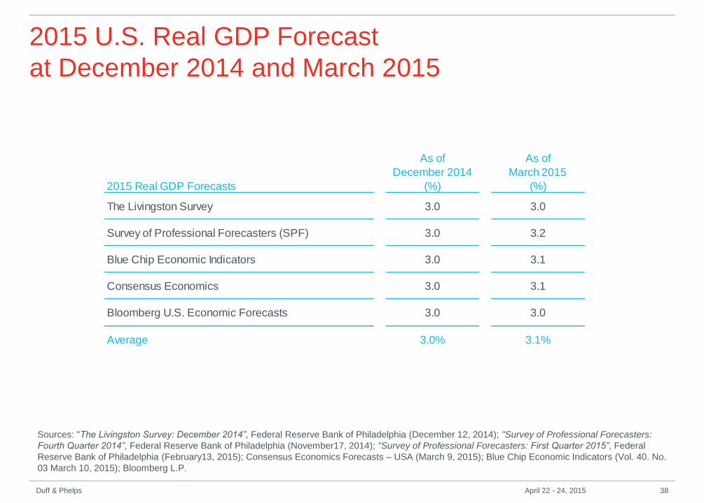
Sources as of December 2014: "The Livingston Survey: December 2014”, Federal Reserve Bank of Philadelphia (December 12, 2014); "Survey of

Professional Forecasters: Fourth Quarter 2014”, Federal Reserve Bank of Philadelphia (November17, 2014); Federal Reserve Bank of Cleveland

(estimates as of December 2014); FRED® Economic Data – Federal Reserve Bank of St. Louis. IHS Outlook Fourth Quarter 2014.

Sources as of March 2015: "Survey of Professional Forecasters: First Quarter 2015”, Federal Reserve Bank of Philadelphia (February 13, 2015); "The

Livingston Survey: December 2014”, Federal Reserve Bank of Philadelphia (December 12, 2014); “US Consensus Forecast “, Consensus Economics Inc.

(March 9, 2015); Blue Chip Economic Indicators (March 10, 2015); Blue Chip Financial Forecasts (March 1, 2015). IHS Outlook First Quarter 2015.


Source

As of

December 2014

(approximately) (%)

As of

March 2015

(approximately) (%)

Livingston Survey

(Federal Reserve Bank of Philadelphia)2.3 2.3

Survey of Professional Forecasters

(Federal Reserve Bank of Philadelphia)2.2 2.1

Cleveland Federal Reserve 1.8 1.7

Blue Chip Financial Forecasts 2.3 2.0

IHS Outlook 2.1 2.1

University of Michigan Survey 5-10 Year Ahead

Inflation Expectations2.8 2.8

Range of Expected Inflation Forecasts 1.8%‒2.8% 1.7%‒2.8%

Methods of Risk-free Rate Normalization – U.S.


As of

December 2014

As of

March 2015

Range of Estimated Long-term Real Rate 1.3% to 2.0% 1.3% to 2.0%

Range of Estimated Expected Inflation Forecasts 1.8% to 2.8% 1.7% to 2.8%

Range of Estimated Long-term Normalized Risk-free Rate 3.1% to 4.8% 3.0% to 4.8%

Midpoint (rounded) 4.0% 4.0%

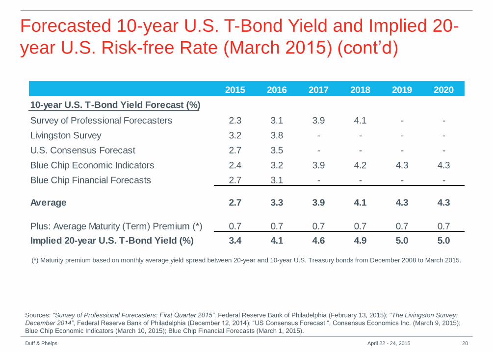
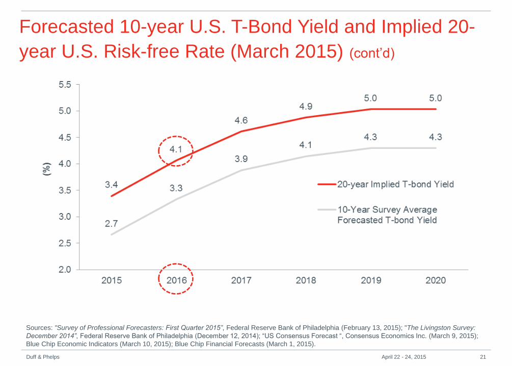
Forecasted 10-year U.S. T-Bond Yield and Implied 20-

year U.S. Risk-free Rate (Dec 2014)

Sources: "Survey of Professional Forecasters: Fourth Quarter 2014”, Federal Reserve Bank of Philadelphia (November17, 2014); "The Livingston Survey:

December 2014”, Federal Reserve Bank of Philadelphia (December 12, 2014); “US Consensus Forecast “, Consensus Economics Inc. (December 8,

2014); Blue Chip Economic Indicators (December 10, 2014); Blue Chip Financial Forecasts (December 1, 2014).

(*) Maturity premium based on monthly average yield spread between 20-year and 10-year U.S. Treasury bonds from December 2008 to December 2014.


2015 2016 2017 2018 2019 2020

10-year U.S. T-Bond Yield Forecast (%)

Survey of Professional Forecasters 2.9 3.4 3.9 - - -

Livingston Survey 3.2 3.8 - - - -

U.S. Consensus Forecast 3.1 3.5 - - - -

Blue Chip Economic Indicators 3.2 3.7 4.3 4.6 4.7 4.7

Blue Chip Financial Forecasts 3.1 - - - - -

Average 3.1 3.6 4.1 4.6 4.7 4.7

Plus: Average Maturity (Term) Premium (*) 0.7 0.7 0.7 0.7 0.7 0.7

Implied 20-year U.S. T-Bond Yield (%) 3.8 4.3 4.8 5.3 5.4 5.4


year U.S. Risk-free Rate (Dec 2014) (cont’d)

Sources: "Survey of Professional Forecasters: Fourth Quarter 2014”, Federal Reserve Bank of Philadelphia (November17, 2014); "The Livingston Survey:

December 2014”, Federal Reserve Bank of Philadelphia (December 12, 2014); “US Consensus Forecast “, Consensus Economics Inc. (December 8,

2014); Blue Chip Economic Indicators (December 10, 2014); Blue Chip Financial Forecasts (December 1, 2014).



year U.S. Risk-free Rate (March 2015) (cont’d)

Sources: "Survey of Professional Forecasters: First Quarter 2015”, Federal Reserve Bank of Philadelphia (February 13, 2015); "The Livingston Survey:

December 2014”, Federal Reserve Bank of Philadelphia (December 12, 2014); “US Consensus Forecast “, Consensus Economics Inc. (March 9, 2015);

Blue Chip Economic Indicators (March 10, 2015); Blue Chip Financial Forecasts (March 1, 2015).

(*) Maturity premium based on monthly average yield spread between 20-year and 10-year U.S. Treasury bonds from December 2008 to March 2015.


2015 2016 2017 2018 2019 2020

10-year U.S. T-Bond Yield Forecast (%)

Survey of Professional Forecasters 2.3 3.1 3.9 4.1 - -

Livingston Survey 3.2 3.8 - - - -

U.S. Consensus Forecast 2.7 3.5 - - - -

Blue Chip Economic Indicators 2.4 3.2 3.9 4.2 4.3 4.3

Blue Chip Financial Forecasts 2.7 3.1 - - - -

Average 2.7 3.3 3.9 4.1 4.3 4.3

Plus: Average Maturity (Term) Premium (*) 0.7 0.7 0.7 0.7 0.7 0.7

Implied 20-year U.S. T-Bond Yield (%) 3.4 4.1 4.6 4.9 5.0 5.0


year U.S. Risk-free Rate (March 2015) (cont’d)


Sources: "Survey of Professional Forecasters: First Quarter 2015”, Federal Reserve Bank of Philadelphia (February 13, 2015); "The Livingston Survey:

December 2014”, Federal Reserve Bank of Philadelphia (December 12, 2014); “US Consensus Forecast “, Consensus Economics Inc. (March 9, 2015);

Blue Chip Economic Indicators (March 10, 2015); Blue Chip Financial Forecasts (March 1, 2015).

German 10-year Bund Yield


Source: Deutsche Bundesbank (http://www.bundesbank.de)

German 15-year Bund Yield


Source: Deutsche Bundesbank (http://www.bundesbank.de)

Long-term Expected Inflation Estimates – Germany

Sources of information: PWC Global Outlook; Germany - IHS Economics and Country Risk; Economist Intelligence Unit; IMF Work Economic Outlook

(WEO).


Source

As of

December 2014

(approximately) (%)

As of

March 2015

(approximately) (%)

PWC Global Outlook 1.7 1.7

IHS Outlook 1.5 1.6

Economist Intelligence Unit 1.8 1.7

IMF World Economic Outlook (WEO) 1.7 1.7

Range of Expected Inflation Forecasts 1.5% to 1.8% 1.6% to 1.7%

Methods of Risk-free Rate Normalization – Germany

* Credit Suisse Global Investment Returns Sourcebook and Yearbook 2015 by Elroy Dimson, Paul Marsh, and Mike Staunton


As of

December 2014

As of

March 2015

Range of Estimated Long-term Real Rate * 1.3% 1.3%

Range of Expected Inflation Forecasts 1.5% to 1.8% 1.6% to 1.7%

Range of Estimated Long-term Normalized Risk-free Rate 2.8% to 3.1% 2.9% to 3.0%

Midpoint (rounded) 3.0% 3.0%

Defining the Equity Risk Premium (ERP)

The ERP (or notational RPm) is defined as:

RPm = Rm – Rf

RPm = Expected equity risk premium

Rm = Expected return on a fully diversified portfolios of equity securities

Rf = Expected rate of return on a risk-free security

The ERP is expectational (i.e., forward-looking) over the expected duration of

the net cash flows.


Unconditional ERP

Unconditional ERP – the long-term average ERP.

Commonly use realized risk premium data (the ex post approach):

While academics and practitioners agree that ERP is a forward-looking

concept, some practitioners, including taxing authorities and regulatory

bodies, use historical data to estimate the ERP under the assumption

that historical data are a valid proxy for current investor expectations –

provides appearance of accuracy.

Estimate of the ERP is the risk premium (realized return on stocks in

excess of the risk-free rate) that investors have, on the average, realized

over some historical holding period

Underlying theory is that the past provides a reasonable indicator of how

the market will behave in the future, and also that investors’ expectations

are influenced by the historical performance of the market


The long-term average of realized risk premiums is calculated from varying rates of

returns on common stocks over shifting risk-free rates.

They are generally reported annually.

It is common practice to add the same long-term average realized risk premium (an

ex post estimate of the ERP) to the market interest rate of the risk-free security

throughout the following year regardless of the level of the rate on that security as of

the valuation date.

This common practice implicitly assumes either that:

1. during upcoming periods the difference between the expected return on

common stocks and U.S. government bonds is constant; or

2. any decrease or increase in the ERP as of the valuation date is short-term

and that the ERP is mean reverting to the long-term average of realized risk

premiums rather quickly.

Unconditional ERP (cont’d)


Problem with relying on unadjusted “Historical” ERP

Source: Morningstar Direct database. Used with permission. Risk-free rate data series used: Long-term Gov't Bonds (IA SBBI US LT Govt YLD USD). As

seen in the 2015 Valuation Handbook – Guide to Cost of Capital.


Realized Equity Risk Premiums:

Stock Market Returns Minus U.S. Government Bonds Through 2014

Source: Data compiled from R. Ibbotson and G. Brinson, Global Investing (New York: McGraw-Hill, 1993); W. Schwert,“Indexes of U.S. Stock Prices from

1802 to 1987, ” Journal of Business Vol. 63 (July 1990): 399–426; S. Homer and R. Sylla, A History of Interest Rates, 3rd ed. (Piscataway, NJ: Rutgers

University Press, 1991); and CRSP and Morningstar Direct database. As seen in the 2015 Valuation Handbook – Guide to Cost of Capital.

Length

(Yrs.) Period Dates

Arithmetic

Average

(%)

Standard

Deviation

(%)

Standard

Error

(%)

Geometric

Average

(%)

20 1995-2014 6.84 19.59 4.38 4.72

30 1985-2014 6.79 17.22 3.14 5.01

40 1975-2014 6.60 16.55 2.62 4.93

50 1965-2014 4.63 16.95 2.40 3.02

89 1926-2014 7.00 20.17 2.14 4.83

115 1900-2014 6.69 19.79 1.85 4.61

143 1872-2014 5.92 18.80 1.57 4.07

217 1798-2014 5.13 17.99 1.22 3.45


Researchers estimating the long-term average ERP adjust average realized risk

premiums for what they believe were non-recurring factors in prior periods or changing

economic conditions.

The years 1942 through 1951 reflected a period of artificial stability in U.S. government

bond interest rates. During World War II, the U.S. Treasury decreed that interest rates

had to be kept at artificially low levels in order to reduce government financing costs.

This led to the Federal Reserve’s April 1942 public commitment to maintain an interest

rate ceiling on government debt, both long term and short term.

After World War II, the Fed continued maintaining an interest rate ceiling, due to the

Treasury’s pressure and, to a lesser extent, a fear of returning to the high

unemployment levels of the Great Depression.

But postwar inflationary pressures caused the Treasury and the Fed to reach an accord

announced March 4, 1951, freeing the Fed of its obligation of pegging interest rates.

The artificially low rates of 1942–1951 creates an upward bias in realized risk premium

data from 1926-2014 of approximately 1.1%

Bias in Realized Risk Premium Data


Realized Risk Premiums

Including and Excluding the Years 1942–1951

Source: Morningstar Direct database. As seen in the 2015 Valuation Handbook – Guide to Cost of Capital.

Period

Dates

Realized Risk Premiums

(arithmetic average) (%)

Standard

Deviations (%)

1926–2014 7.00 20.17

1926–2014 (excluding 1942–1951) 5.89 20.68


Bias in Realized Risk Premium Data (cont’d)

Ibbotson and Chen report on a study in which they estimated forward-looking

long-term sustainable equity returns and expected ERPs since 1926.

In the update to this study, reported in the 2015 Valuation Handbook – Guide to

Cost of Capital, the long-term ERP since 1926 that could have been expected,

given the underlying economics (the “supply side” model estimate), was less

than the historical returns.

Goetzmann and Ibbotson, commenting on the supply side approach of

estimating expected risk premiums, note:

“These forecasts tend to give somewhat lower forecasts than historical risk

premiums, primarily because part of the total returns of the stock market have

come from price-earnings ratio expansion. This expansion is not predicted to

continue indefinitely, and should logically be removed from the expected risk

premium.”


Unconditional ERP Estimates

As reported in the Valuation Handbook – Guide to Cost of Capital:

1926-2013 1926-2014

Long-horizon expected “historical” U.S. equity

risk premium

6.96% 7.00%

Long-horizon expected “historical” U.S. equity

risk premium adjusted for WW II Interest Rate

Bias (excluding 1942–1951)

5.84% 5.89%

Long-horizon expected “supply side” U.S.

equity risk premium

6.18% 6.21%

Long-horizon expected “supply side” U.S.

equity risk premium adjusted for WW II Interest

Rate Bias (excluding 1942–1951)

5.06% 5.10%


ERP is cyclical - conditional ERP represents ERP at specific point in the cycle.

Forward-looking (ex ante) approaches can be grouped into four categories:

Bottom-up implied ERP estimates This is a company-by-company approach. This approach

typically uses expected growth in earnings or dividends as a basis for estimating a “bottom-

up”, company-by-company rate of return for the companies in the universe analyzed.

Top-down implied ERP estimates This approach uses aggregate estimates for the entire

market. This approach typically uses expected growth in earnings or dividends for the

aggregate of the companies comprising a stock index (e.g., the S&P 500), not company-by-

company.

Top-down risk premium estimates This approach estimates the ERP or changes in the ERP

using observed relationships between interest rates or other factors that impact the ERP.

Surveys This approach relies on opinions of investors and financial professionals through

surveys of their views on the prospects of the overall market and the return expected in excess

of a risk-free benchmark.

Conditional ERP


Factors Considered in ERP Recommendation

as of beginning of January 2015

Duff & Phelps Recommended U.S. Equity Risk Premium (ERP) and

Corresponding Risk-Free Rates (Rf): 5.0% (ERP) and matching 4.0% (Rf)

Factor Change Effect on ERP

U.S. Equity Markets ↑ ↓

Implied Equity Volatility ↑ ↑

Corporate Spreads ↑ ↑

GDP Growth and GDP Growth Forecasts ↑ ↓

Unemployment Environment ↓ ↓

Consumer and Business Sentiment ↑ ↓

Sovereign Credit Ratings ↔ ↔

Default Spread Model ↔ ↔

Damodaran Implied ERP Model ↔ ↔


Spread of U.S. High Yield Corporate Bond Yields over

U.S. Investment Grade Corporate Bond Yields January 2011–March 2015

Source: Federal Reserve Bank of St. Louis (FRED)


2015 U.S. Real GDP Forecast

at December 2014 and March 2015

Sources: "The Livingston Survey: December 2014”, Federal Reserve Bank of Philadelphia (December 12, 2014); "Survey of Professional Forecasters:

Fourth Quarter 2014”, Federal Reserve Bank of Philadelphia (November17, 2014); "Survey of Professional Forecasters: First Quarter 2015”, Federal

Reserve Bank of Philadelphia (February13, 2015); Consensus Economics Forecasts – USA (March 9, 2015); Blue Chip Economic Indicators (Vol. 40. No.

03 March 10, 2015); Bloomberg L.P.


2015 Real GDP Forecasts

As of

December 2014

(%)

As of

March 2015

(%)

The Livingston Survey 3.0 3.0

Survey of Professional Forecasters (SPF) 3.0 3.2

Blue Chip Economic Indicators 3.0 3.1

Consensus Economics 3.0 3.1

Bloomberg U.S. Economic Forecasts 3.0 3.0

Average 3.0% 3.1%

U.S. Unemployment Rate: Official (U-3); Unemployment Including

“persons marginally attached to the labor force” (U-6); Civilian Labor Force

Participation Rate

December 1993–March 2015

Source: Federal Reserve Bank of St. Louis (FRED)


University of Michigan Consumer Sentiment Index December 1978–March 2015

Source: Federal Reserve Bank of St. Louis (FRED) and Bloomberg L.P.


Default Spread Model December 2008–March 2015

Source: Morning Direct. Default Spread Model presented herein is based on Jagannathan, Ravi, and Wang, Zhenyu,”The Conditional CAPM and the

Cross-Section of Expected Returns,” The Journal of Finance,Volume 51, Issue 1, March 1996: 3-53. See also Elton, Edwin J. and Gruber, Martin J.,

Agrawal, Deepak, and Mann, Christopher “Is There a Risk Premium in Corporate bonds?”, Working Paper,

http://citeseerx.ist.psu.edu/viewdoc/summary?doi=10.1.1.201.2928


Hassett Risk Premium Factor Model December 2007–March 2015

Source: “S&P 500 Ends 2014 In Fair Value Range With Growth Likely In 2015“ by Steve Hassett. From January 2008 through July 2011 the spot 30-year

risk-free rate is used, thereafter a normalized yield on Treasuries of 4.5% (2% real plus 2.5% inflation) is used. Website:

http://seekingalpha.com/article/2798645-s-and-p-500-ends-2014-in-fair-value-range-with-growth-likely-in-2015


Hassett Risk Premium Factor Model (cont’d)

December 2007–March 2015

Source: “S&P 500 Ends 2014 In Fair Value Range With Growth Likely In 2015“ by Steve Hassett. From January 2008 through July 2011 the spot 30-year

risk-free rate is used, thereafter a normalized yield on Treasuries of 4.5% (2% real plus 2.5% inflation) is used. Website:

http://seekingalpha.com/article/2798645-s-and-p-500-ends-2014-in-fair-value-range-with-growth-likely-in-20150


http://seekingalpha.com/article/2798645-s-and-p-500-ends-2014-in-fair-value-range-with-growth-likely-in-2015?ifp=0

Duff & Phelps Recommended ERP vs.

Arithmetic Adjusted Damodaran Implied ERP

Additional information and data is available at Professor Damodaran’s website at http://pages.stern.nyu.edu/~adamodar/

Professor Aswath Damodaran calculates implied ERP monthly estimates for the

S&P 500 and publishes his estimates on his website.

1. Damodaran estimates an implied ERP by first solving for the discount rate that

equates the current S&P 500 index level with his estimates of cash

distributions (dividends and stock buybacks) in future years.

2. He then subtracts the current yield on 10-year U.S. government bonds to arrive

at the implied ERP.

Duff & Phelps adjust the ERP estimates (based on this model) that Professor

Damodaran publishes since they are geometric average ERP in terms of a 10-year

U.S. Government bond.

Duff & Phelps first converts both of Damodaran’s published geometric ERP

estimates to an equivalent estimate in terms of normalized yields on 20-year U.S.

government bonds and then converts the geometric ERP estimates to their

arithmetic average equivalents.


Duff & Phelps Recommended ERP vs. Arithmetic

Adjusted Damodaran Implied ERP (with Normalized Rf)

at December 2014

Expected growth will vary based on selected cash yield. Additional information and data is available at Professor Damodaran’s website at

http://pages.stern.nyu.edu/~adamodar/


Damodaran

Implied ERP

(as

published)

LTM Cash

Yield

Damodaran

Implied ERP

(as

published)

Normalized

10-year Cash

Yield

Extreme

Case 1:

Lowest Cash

Yield &

Lowest

Expected

Growth Rate

Extreme

Case 2:

Lowest Cash

Yield &

Highest

Expected

Growth Rate

Extreme

Case 3:

Highest

Cash Yield &

Lowest

Expected

Growth Rate

Extreme

Case 4:

Highest

Cash Yield &

Highest

Expected

Growth Rate

Risk Premium Calculator Inputs

Cash yield (dividends and stock buybacks) on Index 4.88% 5.24% 3.47% 3.47% 5.24% 5.24%

Expected Growth Choices (next 5 years) 5.58% 5.58% 4.14% 7.23% 0.92% 7.23%

Long Term Risk Free Rate 2.17% 2.17% 2.17% 2.17% 2.17% 2.17%

Expected growth rate in the long term (after year 5) 2.17% 2.17% 2.17% 2.17% 2.17% 2.17%

Geometric Average Implied ERP 5.78% 6.21% 3.87% 4.43% 5.07% 6.65%

Arithmetic Adjustments:

Normalized RF 4.00% 4.00% 4.00% 4.00% 4.00% 4.00%

Treasury Yield Difference -1.83% -1.83% -1.83% -1.83% -1.83% -1.83%

Geometric Average Implied ERP (Adjusted) 3.95% 4.38% 2.04% 2.60% 3.24% 4.82%

Arithmetic Average ERP Conversion Factor 1.44% 1.44% 1.44% 1.44% 1.44% 1.44%

D&P Arithmetic Adjusted Implied ERP 5.39% 5.81% 3.48% 4.03% 4.67% 6.25%


Adjusted Damodaran Implied ERP (with Normalized Rf)

at March 2015

Expected growth will vary based on selected cash yield. Additional information and data is available at Professor Damodaran’s website at

http://pages.stern.nyu.edu/~adamodar/


Damodaran

Implied ERP

(as

published)

LTM Cash

Yield

Damodaran

Implied ERP

(as

published)

Normalized

10-year Cash

Yield

Extreme

Case 1:

Lowest Cash

Yield &

Lowest

Expected

Growth Rate

Extreme

Case 2:

Lowest Cash

Yield &

Highest

Expected

Growth Rate

Extreme

Case 3:

Highest

Cash Yield &

Lowest

Expected

Growth Rate

Extreme

Case 4:

Highest

Cash Yield &

Highest

Expected

Growth Rate

Risk Premium Calculator Inputs

Cash yield (dividends and stock buybacks) on Index 4.93% 5.25% 3.45% 3.45% 5.25% 5.25%

Expected Growth Choices (next 5 years) 5.48% 5.48% 4.27% 7.13% 1.02% 7.13%

Long Term Risk Free Rate 1.93% 1.93% 1.93% 1.93% 1.93% 1.93%

Expected growth rate in the long term (after year 5) 1.93% 1.93% 1.93% 1.93% 1.93% 1.93%

Geometric Average Implied ERP 5.86% 6.24% 3.91% 4.43% 5.14% 6.68%

Arithmetic Adjustments:

Normalized RF 4.00% 4.00% 4.00% 4.00% 4.00% 4.00%

Treasury Yield Difference -2.07% -2.07% -2.07% -2.07% -2.07% -2.07%

Geometric Average Implied ERP (Adjusted) 3.79% 4.17% 1.84% 2.36% 3.07% 4.61%

Arithmetic Average ERP Conversion Factor 1.44% 1.44% 1.44% 1.44% 1.44% 1.44%

D&P Arithmetic Adjusted Implied ERP 5.23% 5.61% 3.28% 3.80% 4.51% 6.05%


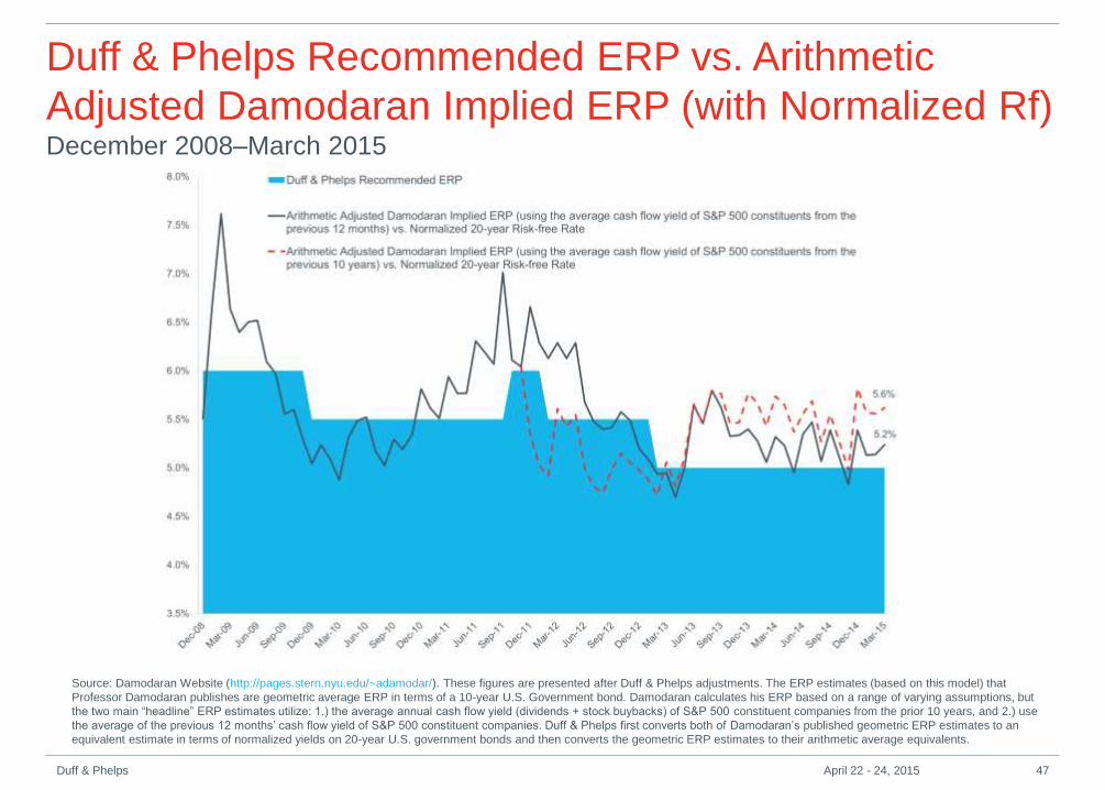
Adjusted Damodaran Implied ERP (with Normalized Rf) December 2008–March 2015

Source: Damodaran Website (http://pages.stern.nyu.edu/~adamodar/). These figures are presented after Duff & Phelps adjustments. The ERP estimates (based on this model) that

Professor Damodaran publishes are geometric average ERP in terms of a 10-year U.S. Government bond. Damodaran calculates his ERP based on a range of varying assumptions, but

the two main “headline” ERP estimates utilize: 1.) the average annual cash flow yield (dividends + stock buybacks) of S&P 500 constituent companies from the prior 10 years, and 2.) use

the average of the previous 12 months’ cash flow yield of S&P 500 constituent companies. Duff & Phelps first converts both of Damodaran’s published geometric ERP estimates to an

equivalent estimate in terms of normalized yields on 20-year U.S. government bonds and then converts the geometric ERP estimates to their arithmetic average equivalents.



Adjusted Damodaran Implied ERP (with Spot Rf) December 2008–March 2015

Source: Damodaran Website (http://pages.stern.nyu.edu/~adamodar/). These figures are presented after Duff & Phelps adjustments. The ERP estimates (based on this model) that

Professor Damodaran publishes are geometric average ERP in terms of a 10-year U.S. Government bond. Damodaran calculates his ERP based on a range of varying assumptions, but the

two main “headline” ERP estimates utilize: 1.) the average annual cash flow yield (dividends + stock buybacks) of S&P 500 constituent companies from the prior 10 years, and 2.) use the

average of the previous 12 months’ cash flow yield of S&P 500 constituent companies. Duff & Phelps first converts both of Damodaran’s published geometric ERP estimates to an

equivalent estimate in terms of actual yields on 20-year U.S. government bonds and then converts the geometric ERP estimates to their arithmetic average equivalents.


Reported in the 2015 Valuation Handbook ‒ Guide to Cost of

Capital:

The Duff & Phelps Recommended ERP as of December 31,

2014 is 5.0%

Developed in relation to (and should be used in conjunction

with) a 4.0% normalized) risk-free rate.

Conditional ERP Estimates

This implies a “base” U.S. cost of equity of 9.0% (5.0% + 4.0%)

as of December 31, 2014.


Duff & Phelps Recommended U.S. ERP and

Corresponding Risk-free Rates January 2008–Present

Duff & Phelps

Recommended ERP Risk-Free Rate

Year-end 2014 Guidance

December 31, 20145.0%

4.0%

Normalized 20-year Treasury yield *


December 31, 20135.0%

4.0%


January 1, 2013 − February 27, 2013 5.5%4.0%



December 31, 20125.5%

4.0%


Change in ERP Guidance

January 15, 2012 − February 27, 20135.5%

4.0%



September 30, 2011 − January 14, 20126.0%

4.0%


July 1 2011 − September 29, 2011 5.5%4.0%


June 1, 2011 − June 30, 2011 5.5%Spot

20-year Treasury Yield

May 1, 2011 − May 31, 2011 5.5%4.0%


December 1, 2010 − April 30, 2011 5.5%Spot


June 1, 2010 − November 30, 2010 5.5%4.0%



December 1, 2009 − May 31, 20105.5%

Spot


* Normalized in this context means that in months where the risk-free rate is deemed to be abnormally low, a proxy for a longer-term sustainable risk-free

rate is used. As seen in the 2015 Valuation Handbook – Guide to Cost of Capital


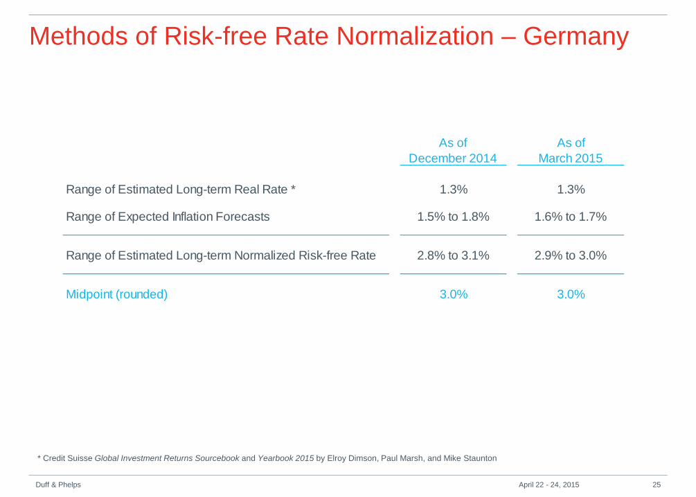
Conditional ERP Estimate with a Normalized Risk-free Rate –

Germany

ERP as of December 31, 2014 = 5.5%

matched with a normalized risk-free rate* = 3.5%

(Base cost of equity capital, rounded = 9.0%)

ERP as of March 31, 2015 = 5.5%

matched with a normalized risk-free rate* = 3.5%

(Base cost of equity capital, rounded = 9.0%)


* Based on the consideration of the risk-free rate build up and long-term historical moving average. 30-year German bund yield spot risk-free rate as of December 31,

2014 and March 31, 2015 was 1.37% and 0.58%, respectively.

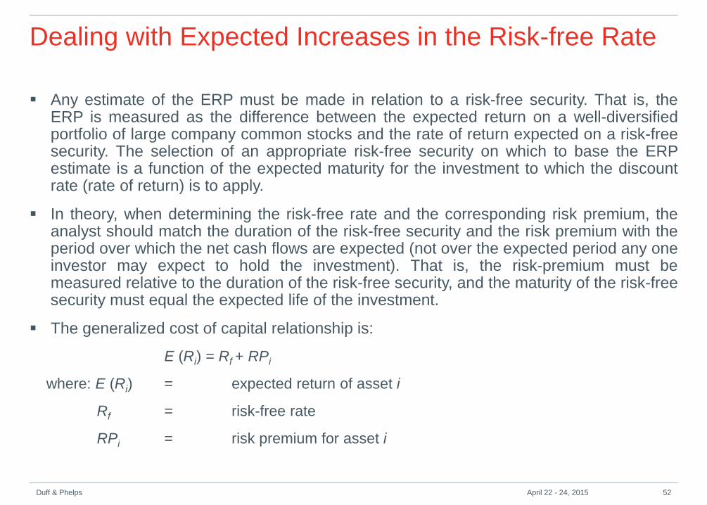
Dealing with Expected Increases in the Risk-free Rate

Any estimate of the ERP must be made in relation to a risk-free security. That is, the

ERP is measured as the difference between the expected return on a well-diversified portfolio of large company common stocks and the rate of return expected on a risk-free security. The selection of an appropriate risk-free security on which to base the ERP estimate is a function of the expected maturity for the investment to which the discount rate (rate of return) is to apply.

In theory, when determining the risk-free rate and the corresponding risk premium, the analyst should match the duration of the risk-free security and the risk premium with the period over which the net cash flows are expected (not over the expected period any one investor may expect to hold the investment). That is, the risk-premium must be measured relative to the duration of the risk-free security, and the maturity of the risk-free security must equal the expected life of the investment.

The generalized cost of capital relationship is:

E (Ri) = Rf + RPi

where: E (Ri) = expected return of asset i

Rf = risk-free rate

RPi = risk premium for asset i


Dealing with Expected Increases in the Risk-free Rate (cont’d)

As a short-cut, analysts often use the maturity of the risk-free instrument instead of

the duration as the expected life of the investment. Often this makes little difference.

For example, if you were estimating the expected equity return on a highly liquid investment with an expected short-term maturity, a U.S. government short-term note (e.g., T-bill) may be an appropriate instrument to use in benchmarking a risk premium.

Alternatively, if you were estimating the equity return on a long-term investment such as the valuation of a business where the value can be equated to the present value of a series of future cash flows over many years, then the yield on a long-term U.S. government bond (e.g., T-bond) may be the more appropriate instrument in benchmarking a risk premium.

Assuming that the risk premium is a function of a relative risk measure, β, multiplied by the equity risk premium (notationally RPm), the analyst should be discounting expected cash flows as follows:

Note: We are using the term β here to indicate a generalized relative risk measure; that is, it measures how the returns of the respective investment are expected to vary relative to changes in returns on the market. For simplicity, we are assuming β is constant.


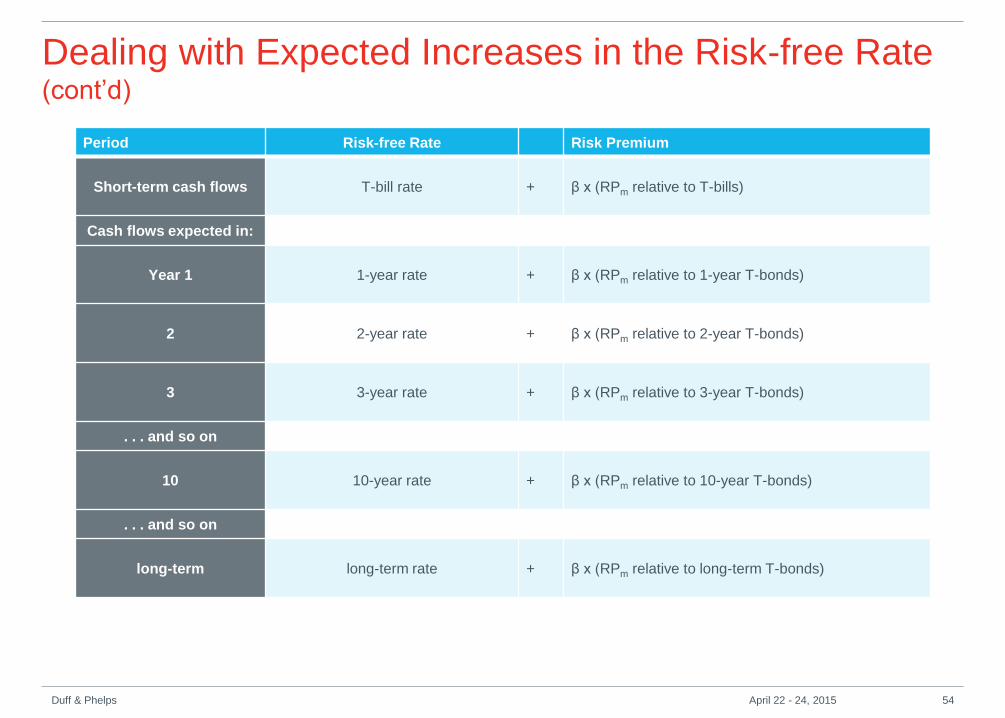
Dealing with Expected Increases in the Risk-free Rate (cont’d)

Period Risk-free Rate Risk Premium

Short-term cash flows T-bill rate + β x (RPm relative to T-bills)

Cash flows expected in:

Year 1 1-year rate + β x (RPm relative to 1-year T-bonds)

2 2-year rate + β x (RPm relative to 2-year T-bonds)


. . . and so on


. . . and so on

long-term long-term rate + β x (RPm relative to long-term T-bonds)


Baker, Wurgler, Bradley, “A Behavioral Finance Explanation for the Success of Low

Volatility Portfolios”, NYU Working Paper No. 2451/29537.

http://ssrn.com/abstract=2284643http://ssrn.com/abstract=2284643

Over last 40 years, high volatility and high beta stocks have substantially

underperformed low volatility and low beta stocks

In an inefficient market, “mispricing” comes from:

– Some investors not fully rational – prefer lotteries (prefer positive skewness

of low priced, high volatile stocks) representativeness (assumes one can pick

out winners among start-up companies while ignoring high probability of

failure) overconfidence (confidence intervals too narrow – overconfidence in

accuracy of knowledge)

– Limits to arbitrage – high volatility/high beta stocks should be “shorted” but

these are generally small cap, costly to trade and difficult to short

Issue: are the assumptions of CAPM violated?




Issue: do we know how to measure beta?

While beta is a forward concept, our tools to estimate beta are based on

look-back methods. This can create errors in the estimation.

For example, assume the subject business had become distressed and had

recently emerged from restructuring its debt and an infusion of equity. The

following exhibit presents an example of an adjustment in pricing for a stock

of this hypothetical company.

In period A, the company returns had essentially moved with the market. In

period B, the company is distressed, and its stock is experiencing a

downward repricing. During this period, the company’s returns are not

correlated with the movement of the overall market at all. In period C, the

restructuring of the company and the repricing of the company’s stock is

complete, and the company’s returns are once again moving more in

tandem with market returns.


Issue: do we know how to measure beta? (cont’d)

0.0000

0.2000

0.4000

0.6000

0.8000

1.0000

1.2000

1.4000

1.6000

Co

mp

ou

nd

Re

turn

Time

Example Company Vs. Index

Over Time

Example S&P 500

A B C

1 2


If one were to compute beta at time 1, which includes period A as the look-

back period, the beta estimate would reflect a normal relationship between

the company’s returns and the market’s returns. In fact, its beta estimate

would be near 1.

In contrast, computing a beta estimate at time 2, which includes period B

(the period of the company’s stock repricing) as the look-back period,

would not yield a reliable forward-looking beta estimate. In fact, it would

yield a beta estimate lower than expected since the company’s return was

negative in a period when the market’s return was generally positive. This

result is counterintuitive, given the company’s downward repricing; that is,

the operating risk of the company has not declined over period B, and in

fact, its operating risk was greatest during this period.

Once the restructuring of the company and the repricing of the company’s

stock is complete, its normal relationship to the market will resume in

period C.



To estimate beta at time 2 for the company, one should use a bottom-up beta

estimate because a top-down estimate will result in an erroneous beta

estimate.

Using betas of guideline public companies for estimating a bottom-up beta

has been found to provide reasonably accurate estimates of the subject

company.

The more guideline companies used in the sample size, the better the

accuracy. The accuracy is also enhanced if the guideline public companies

are reasonably close in size to the subject company. When the guideline

public companies are larger than the subject company, the beta estimate for

the subject company is biased low, because of the propensity of betas of

larger companies to be smaller than the betas of smaller companies.

Use of the beta estimate derived from guideline public companies larger than

the subject company will generally result in too low an estimate of the cost of

equity capital. Hence, one needs to consider adjusting for the size effect.



Issue: do the formulas for unlevering and levering

equity betas reflect the market?

Published and calculated betas for publicly traded stocks typically reflect the

capital structure of each respective company at market values.

These betas sometimes are referred to as levered betas, betas reflecting the

leverage in the company’s capital structure.

Levered betas incorporate two risk factors that bear on systematic risk:

1. business (or operating) risk and

2. financial (or capital structure) risk.

Removing the effect of financial leverage (i.e., unlevering the beta) leaves

the effect of business risk only (“asset beta”).


Issue: how does the market price risk?

Exhibit 21.5 Beta as a Function of Leverage

Source: Arthur G. Korteweg, “The Costs of Financial Distress across Industries,” Working paper, Stanford

University, January 15, 2007, 65. Used with permission. All rights reserved.

Be

ta

Weighted average beta of equity and debt

Bd

BL


Ri = Rf + Bi,m RPm + Bi,s RPi,s + Bi,BV RPi,BV + … + Bi,u RPi,u + …+ εi

where:

Ri = Realized return for stock of company i

Rf = Risk-free rate of return

Bi,m = Sensitivity of return of stock of company i to the market risk premium, RPm (ERP)

Bi,s = Sensitivity of return of stock of company i to a measure of size, S, of company i and Si = Measure of size of company i

RPi,s = Bi,s x Si = Risk premium for size of company i

Bi,BV = Sensitivity of return of stock of company i to a measure of BV (typically measure of book-value-to- market-value) of stock of company i and BVi

RPi,BV = Bi,BV x BVi = Risk premium for book value of company i

… = Other factors

Bi,u = Sensitivity of return of stock of company i to a measure of unique risk of company i

Ui = Measure of unique risk of company i

RPi,u = Bi,u x Ui = Risk premium for unique risk of company i

εi = Error term, difference between predicted return and realized return.

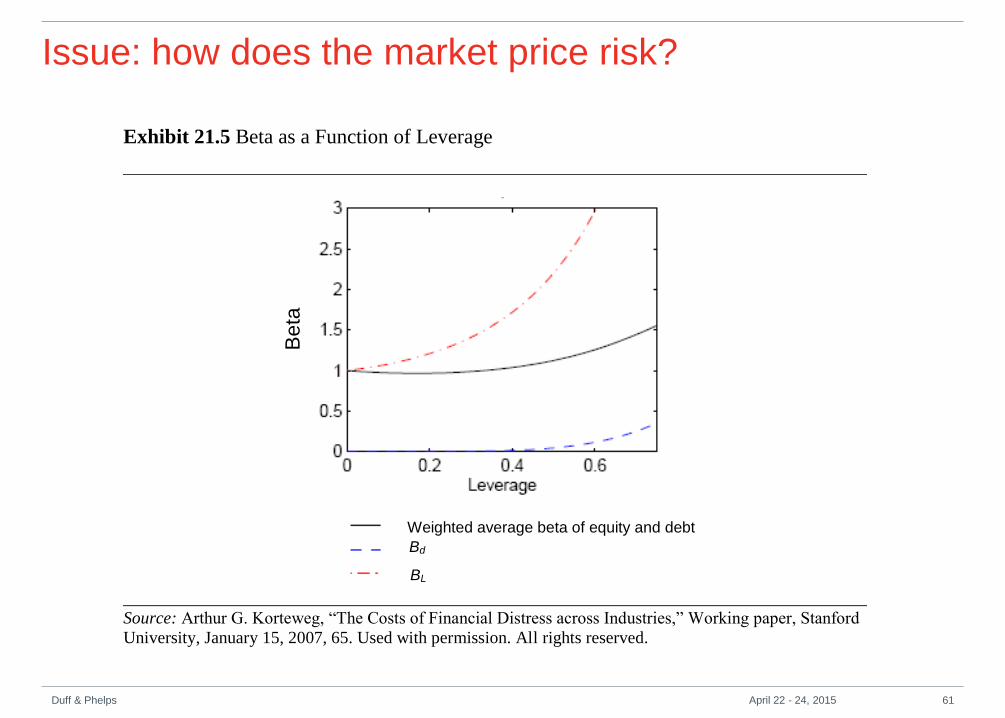
Issue: is the market pricing more systematic factors?


Modified CAPM Cost of Capital Formula

Modifying CAPM, we can expand the cost of equity capital formula to

add two correction factors – size effect and company-specific risk:

If you do not modify CAPM do you believe in the pure CAPM?


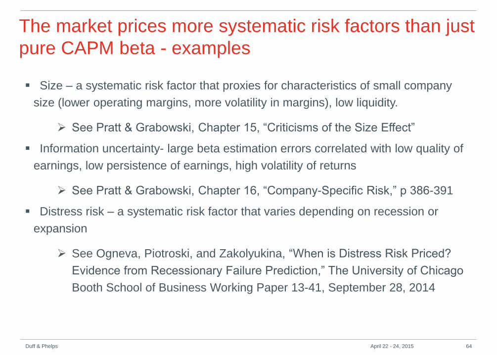
The market prices more systematic risk factors than just

pure CAPM beta - examples

Size – a systematic risk factor that proxies for characteristics of small company

size (lower operating margins, more volatility in margins), low liquidity.

See Pratt & Grabowski, Chapter 15, “Criticisms of the Size Effect”

Information uncertainty- large beta estimation errors correlated with low quality of

earnings, low persistence of earnings, high volatility of returns

See Pratt & Grabowski, Chapter 16, “Company-Specific Risk,” p 386-391

Distress risk – a systematic risk factor that varies depending on recession or

expansion

See Ogneva, Piotroski, and Zakolyukina, “When is Distress Risk Priced?

Evidence from Recessionary Failure Prediction,” The University of Chicago

Booth School of Business Working Paper 13-41, September 28, 2014


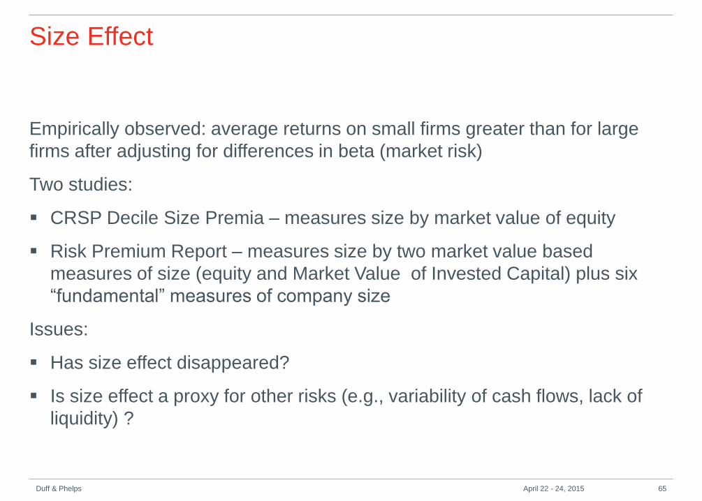
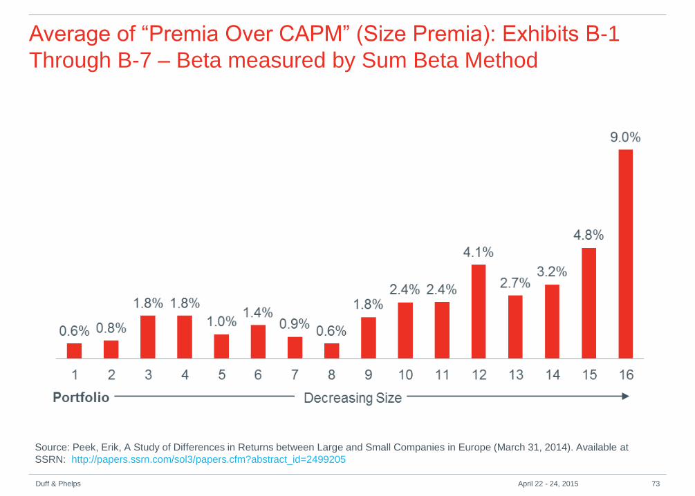
Empirically observed: average returns on small firms greater than for large

firms after adjusting for differences in beta (market risk)

Two studies:

CRSP Decile Size Premia – measures size by market value of equity

Risk Premium Report – measures size by two market value based

measures of size (equity and Market Value of Invested Capital) plus six

“fundamental” measures of company size

Issues:

Has size effect disappeared?

Is size effect a proxy for other risks (e.g., variability of cash flows, lack of

liquidity) ?

Size Effect


Sources of underlying data: 1.) CRSP U.S. Stock Database and CRSP U.S. Indices Database © 2014 Center for Research in Security

Prices (CRSP®), University of Chicago Booth School of Business. 2.) Morningstar EnCorr database. Used with permission. All rights

reserved. Calculations performed by Duff & Phelps LLC.

Risk-free Rate (Rf) Security Market Line (SML)

SP SP

Size Effect Over Recent Time Periods Alternative Measures of Size – Market Capitalization

Risk Premium Report - Size Study: 1963-2014, 1990-2014


Risk-free Rate (Rf) Security Market Line (SML)

SP SP

Size Effect Over Recent Time Periods Alternative Measures of Size – 5-Year Average Net Income

Risk Premium Report - Size Study: 1963-2014, 1990-2014

Sources of underlying data: 1.) CRSP U.S. Stock Database and CRSP U.S. Indices Database © 2014 Center for Research in Security

Prices (CRSP®), University of Chicago Booth School of Business. 2.) Morningstar EnCorr database. Used with permission. All rights

reserved. Calculations performed by Duff & Phelps LLC.


Portfolio 25

Differences in Returns Between Large and Small

Companies in Europe

This study is published as part of the ongoing research that Duff &

Phelps performs and sponsors in the area cost of capital and other

valuation issues.

This study consists of a (i) a Research Note and (ii) a set of Sample

Exhibits.

The full Research Note “Differences in Returns Between Large and

Small Companies in Europe”, is available at


Erik Peek is the Duff & Phelps Professor of Business Analysis &

Valuation at Rotterdam School of Management, Erasmus University

(RSM).



Companies in Europe (cont’d)

Research Note: The broad conclusions of this analysis were:

Using various measures of firm size, the findings suggest that small stocks

have outperformed large stocks, on average, suggesting that in Europe

investors perceive small firms as more risky and thus demand a size

premium.

The evidence also indicates that the relationship between firm size and

returns is strongly non-linear, and that the size premium is significant only

for the smallest companies.

The relationship between firm size and returns likely varies across regions.

Size premiums in Ireland, the United Kingdom, and the Nordic countries

(Denmark, Finland, Norway, and Sweden) appear to be statistically

significant, while the size premiums in the other European countries

studied may not be significant.



Companies in Europe (cont’d)

As such, the results of the Research Note were mixed. This does not

automatically imply that firm size does not matter for cost of capital estimation

in some countries ‒ splitting up the sample unavoidably affects the statistical

power of the study’s tests and tends to reduce statistical significance in at

least some of the subsamples.

Leaving aside statistical significance, the Research Note’s findings suggest

that the average return spread between small and large firms is positive in

each of the examined regional subsamples, and that size and liquidity

distributions likely differ across regions.

Professor Peek posits that such differences may potentially explain why the

size effect appears strong in some regions but less strong in others.



Companies in Europe: Countries Included

Austria Luxembourg

Belgium The Netherlands

Denmark Norway

Finland Portugal

France Spain

Germany Sweden

Greece Switzerland

Ireland United Kingdom

Italy


Average Annual Return Spreads Between Top and Bottom

Market Capitalization Quartiles by Country or Region


Source: Peek, Erik, A Study of Differences in Returns between Large and Small Companies in Europe (March 31, 2014). Available at

SSRN: http://papers.ssrn.com/sol3/papers.cfm?abstract_id=2499205

Average of “Premia Over CAPM” (Size Premia): Exhibits B-1

Through B-7 – Beta measured by Sum Beta Method


Source: Peek, Erik, A Study of Differences in Returns between Large and Small Companies in Europe (March 31, 2014). Available at

SSRN: http://papers.ssrn.com/sol3/papers.cfm?abstract_id=2499205

Companies Ranked by Size Factor Premia over CAPM (Size Premia, RP s ) Exhibit B-7Historical Equity Risk Premium: Average Since 1990 Equity Risk Premium Study: Data through December 31, 2013

Data for Year Ending December 31, 2013 Data Smoothing with Regression Analysis

Dependent Variable: Premium over CAPM

Sum Beta Independent Variable: Log of Average Size Factor

Smoothed

Portfolio Avg. Log of Beta Arithmetic Indicated Premium t-Value Premium Regression Output:

Rank Size Factor Avg. (Sum Beta) Avg. Risk CAPM over Premium over

by Size (in € millions) Size Factor Since '90 Premium Premium CAPM over CAPM CAPM Intercept 1.228%

Log(Size) -0.528%

1 (big) 2.40 – 0.95 5.28% 4.59% 0.69% – 0.29% Log(Size)2 1.323%

2 1.60 – 1.04 5.10% 5.03% 0.07% -0.495 1.61% Log(Size)3 -0.528%

3 1.20 – 1.04 7.23% 5.03% 2.20% 0.894 1.59% Adj. R2 70%

4 0.90 – 1.07 7.66% 5.17% 2.49% 0.911 1.44%

5 0.60 – 1.06 6.07% 5.12% 0.95% 0.089 1.27%

6 0.40 – 1.06 6.68% 5.12% 1.56% 0.372 1.20%

7 0.20 – 1.03 5.45% 4.98% 0.47% -0.122 1.17%

8 0.00 – 1.05 4.90% 5.08% -0.17% -0.478 1.23%

9 (0.20) – 1.00 7.00% 4.83% 2.17% 0.706 1.39%

10 (0.40) – 0.97 7.35% 4.69% 2.66% 1.044 1.69%

11 (0.50) – 1.02 6.93% 4.93% 2.00% 0.596 1.89%

12 (0.70) – 0.92 9.34% 4.45% 4.89% 1.962 2.43%

13 (0.90) – 0.99 7.10% 4.79% 2.32% 0.712 3.16%

14 (1.10) – 1.02 5.87% 4.93% 0.94% 0.099 4.11%

15 (1.40) – 1.07 11.89% 5.17% 6.72% 2.181 6.01%

16 (small) (1.80) – 1.31 16.39% 6.33% 10.06% 1.955 9.54%

© 2014 Duff & Phelps, LLC Differences in Returns Between Large and Small Companies in Europe (2014)

Source of underlying data: Thomson Reuters Datastream and Worldscope.

Used with permission. All rights reserved.

Smoothed Premium = 1.228% -0.528% * Log(Size Factor) +

1.323% * Log(Size Factor)^2 -0.528% * Log(Size Factor)^3

-2%

0%

2%

4%

6%

8%

10%

12%

-3.0 -2.0 -1.0 0.0 1.0 2.0 3.0

Pre

miu

m o

ver

CA

PM

Size Factor

Smoothed Premium over CAPM vs. Unadjusted Premium over CAPM


Risk in Projections

Management prepared forecasts: The analysts’ first task is to test the forecasts

to determine if forecasts prepared in prior periods have consistently been

biased: are the forecast aspirational or expectational.

That is, do they represent management’s belief as to what can be

accomplished if they succeed in carrying out their business plan. Businessmen

by their nature are optimists. Rarely are the projections tempered for possible

downside outcomes.

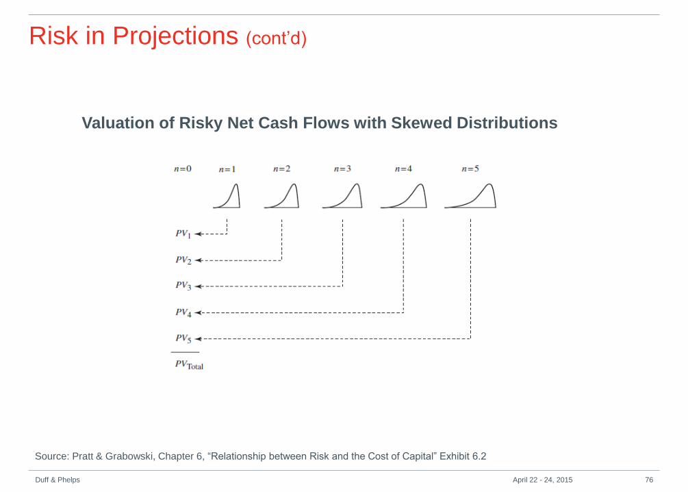
The following exhibit graphically displays the valuation process where net cash

flows are represented by skewed distributions of possible outcomes. In the

short-term, year-by-year, the distributions of net cash flows are likely skewed.

Upside possibilities are limited by available resources while downside

possibilities are only limited by the backlog of orders carried over from prior

periods.


Risk in Projections (cont’d)

Source: Pratt & Grabowski, Chapter 6, “Relationship between Risk and the Cost of Capital” Exhibit 6.2


Valuation of Risky Net Cash Flows with Skewed Distributions


The premise of developing discount rates is to estimate the risk of an investment

and applying those discount rates to the expected cash flows of the investment,

which results in an estimate of value.

Expected cash flows should account for downside scenarios, of course, but

sometimes the forecasts prepared by management and used in a valuation can

be somewhat rosy in that they may reflect successful outcomes only, rather than

reflecting the range of possible outcomes (both good and bad) that should be

included in estimated expected cash flows.

Adding a C-SRP to the discount rate is a commonly applied method to account for the

overly optimistic forecasts provided to the analyst. For example, in the context of the

modified CAPM we get the following:

E(Ri) – Rf + Beta x ERP + RPs

+ RPc (C-SRP due to biased cash flow estimates)



Forecasts may also be biased high because they do not take into account the

possibility that cash flows will in fact stop because of a possible downside risk that

simply causes the business to stop operating (e.g., loss of the contract with the

sole customer of the business).

But, developing a probability analysis of possible net cash flows with one of the

outcomes net cash flows equal to zero can assist the analyst in understanding the

relative magnitude of his or her subjective assessment of the risk represented by

the addition of a C-SRP.

We recommend that an analyst examine the probability of a zero net cash flow

scenario in the distribution of possible net cash flows as a check on any C-SRP

added to the discount rate to account for the chance that the subject company

may be forced to shut down because of a company-specific risk factor.


Risk Differences Often Cannot Be Adjusted for in Net

Cash Flows According to the generally held theory surrounding using CAPM as the basis for estimating the cost of capital (for example), bad outcomes should be reflected in the various possible cash flows with the expected cash flows reflecting both the more likely scenarios but also scenarios that will have a negative impact on net cash flows.

But adjusting the mean of the cash flow distribution does not adjust for differences in the distribution itself.

Examples of companies with likely different variability of possible net cash flow outcomes compared to the guideline public companies:

Drug companies: stage of development of testing and approval of subject company differ from guideline companies which have many drugs at various stages of their life cycles;

Entertainment company (films, TV stations, radio stations): guideline companies more geographically and outlet diversified than subject company.

Examine the dispersion of operating cash flows- is the dispersion greater for the subject company than for the guideline public companies? If “yes”, more operating risk and greater cost of capital.


Common Mistakes in Estimating Overall Cost of Capital

(WACC)

Relying on simple WACC formula

• While the WACC is by far the most widely used discount rate for

valuing the business enterprise, the WACC handling of income tax

issues is simplistic and ignores investor level taxes and capital gains

treatment that are important considerations in the valuing of pass-

through entities.

• Implicitly, the interest tax shield equals the cost of debt capital times

the market value of debt and assumes that the income tax deductions

from interest expense result in reduced cash income taxes in the

period in which the interest is paid.

• There may be a risk of realizing the interest tax shield.


Common mistakes that we believe are made when the value of an M&A

transaction is being assessed:

Using the acquiring firm’s overall cost of capital to value the

acquisition. The correct cost of capital matches the risks of the

expected cash flows being valued.

Basing the cost of capital to value an acquisition on the cost of the

capital used to finance the acquisition.

For example, a large strategic acquirer may make a small acquisition

using all debt and analyze the transaction based on its cost of debt. This

may be the cost incurred by the acquirer but not the appropriate cost of

capital to assess the value of the acquisition.

Common Mistakes in M&A


The cost of capital of an acquisition should reflect the risk of the target, not the risk of the buyer.

Value and Price Differ:

Pricing can be thought of as a three-pronged analysis:

1. Start with stand-alone analysis.

2. Layer in synergies that likely bidders (sometimes termed the pool of willing buyers or market participants) may need to give away to the target owners to get the transaction done.

3. Any of these synergies are due to the market participant characteristics, not the risk characteristics of the target; these can include cash flow synergies and risk (discount rate) synergies.

4. Layer in your specific synergies, which again can include cash flow synergies and risk (discount rate) synergies.

Common Mistakes in M&A (cont’d)



Adding the value of synergies to the stand-alone value to determine a

price for the target by sharing any of these synergies is due to the

bidder consciously giving up some of its value to the target’s owners.

But in no case is the correct cost of capital the cost of capital of the

buyer.

The buyer has its own portfolio of operations with their risks reflected in

the buyer’s cost of capital. Those risks may be the same as those of the

target, but that is a chance event.



Failure to differentiate the risks of the different cash flow stream

categories (i.e., integration costs, target company operating cash

flows, and synergies). Cash flows from synergies are typically riskier

than the target company’s stand-alone operating cash flows and

integration costs.


Contact Information

Roger Grabowski, FASA

Managing Director

Valuation Advisory

+1 312 697 4720

[email protected]


Duff & Phelps

Valuation Handbook series Published by John Wiley & Sons, Inc.

Company Level Cost of Capital Data

Morningstar/Ibbotson

SBBI Valuation Yearbook

(discontinued) 2015 Valuation Handbook ‒ Guide to

Cost of Capital

Company-level Cost of Capital


Where to Purchase

The 2015 Valuation Handbook is available from:

John Wiley & Sons

www.wiley.com/go/ValuationHandbooks

Or through one of the distributors:

AICPA Business Valuation Resources www.cpa2biz.com www.bvresources.com/costofcapital

1-(888) 777-7077 1-(503) 291-7963 ext. 2

[email protected] 2015 Valuation Handbook and ToolKit (formerly the Calculator)

ValuSource

www.valusource.com/vhb

1 (800) 825-8763

The Valuation Handbook was released March 11, 2015.

Valuation Handbook- Guide to Cost of Capital


http://www.wiley.com/go/ValuationHandbooks

http://www.cpa2biz.com/

http://www.bvresources.com/costofcapital

mailto:[email protected]

http://www.valusource.com/vhb

Industry Level Cost of Capital Data


What is the difference between

(i) annual Valuation Handbook – Guide to Cost of Capital and

(ii) annual Valuation Handbook – Industry Cost of Capital ?

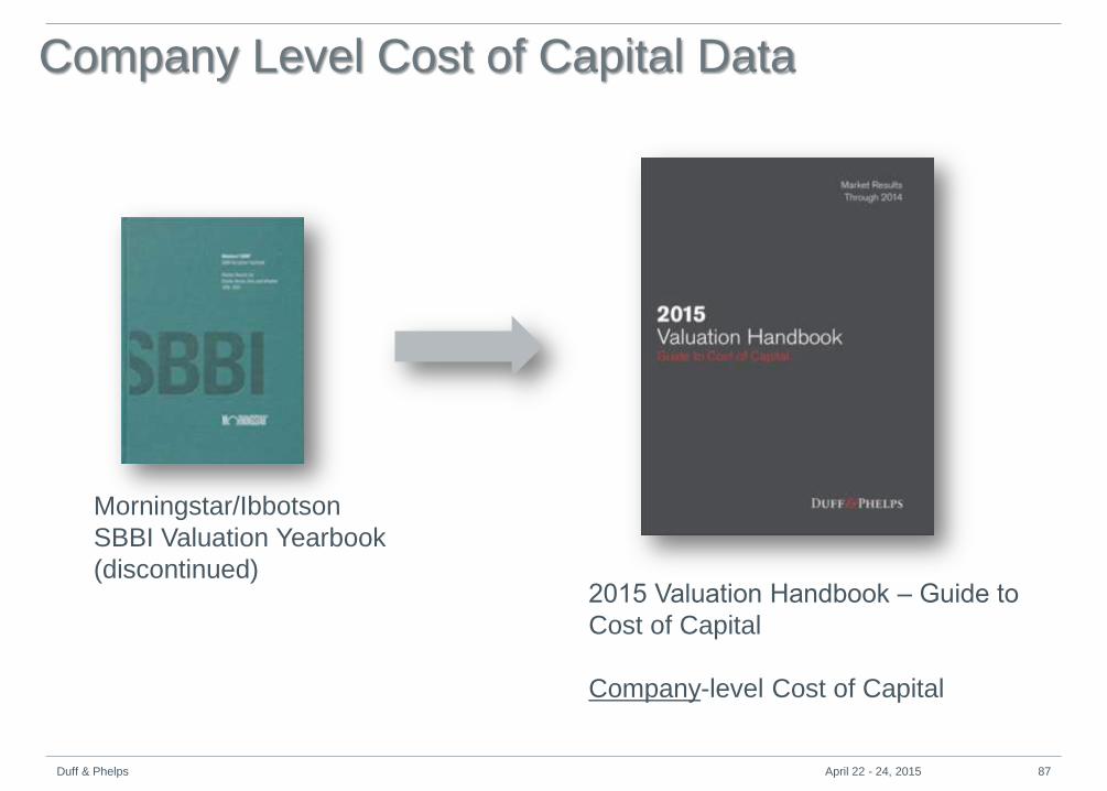
The Valuation Handbook – Guide to Cost of Capital is the book that includes all

the key data from the (now discontinued) Morningstar/Ibbotson SBBI Valuation

Yearbook and the Risk Premium Report.

• Data through December, with optional March, June, and September quarterly

updates.


What is the difference between

(i) annual Valuation Handbook – Guide to Cost of Capital and

(ii) annual Valuation Handbook – Industry Cost of Capital ?

The Valuation Handbook – Industry Cost of Capital is the book that

includes industry data, similar to the (now discontinued)

Morningstar/Ibbotson Cost of Capital Yearbook.

Data through March, with optional June, September, and December

quarterly updates.


• Industry Cost of Capital Estimates

• Industry Valuation Multiples

• Industry Levered and Unlevered Betas

• Analysis of Off-Balance-Sheet Debt by Industry

* Depending on data availability; some industries may not include all estimates.

The Valuation Handbook ‒ Industry Cost of

Capital…What’s in it?


Sample Industry Page

The Valuation Handbook ‒

Industry Cost of Capital

includes analysis of

• Over 200 U.S. industries

• And 4 size groupings (large-,

mid-, low-, and micro-cap

stocks)


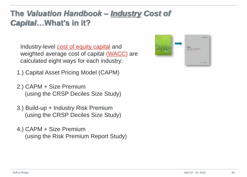
1.) Capital Asset Pricing Model (CAPM)

2.) CAPM + Size Premium

(using the CRSP Deciles Size Study)

3.) Build-up + Industry Risk Premium

(using the CRSP Deciles Size Study)

4.) CAPM + Size Premium

(using the Risk Premium Report Study)

Industry-level cost of equity capital and

weighted average cost of capital (WACC) are

calculated eight ways for each industry:




Industry-level cost of equity capital and

weighted average cost of capital (WACC) are

calculated eight ways for each industry:



5.) Build-up + Risk Premium Over the Risk-free Rate

(using Risk Premium Report Study)

6.) 1-Stage Discounted Cash Flow (DCF) model

7.) 3-Stage DCF model

8.) Fama-French (F-F) Factor Model


Valuation Multiples

• Price to Earnings

• Price to Book

• Market to Book

• Enterprise Value to Sales

• Enterprise Value to EBITDA

• Capital Structure

Industry-level valuation multiples and capital

structure statistics are calculated for each

industry:

Capital Structure

• Capital structure

• Debt to Equity

• Debt to Total Capital




• Raw (OLS) betas

• Blume-adjusted betas

• Peer group betas

• Vasicek-adjusted betas

• Sum betas

• Downside betas

Levered and unlevered betas for each industry:

If you use the capital asset

pricing model, you need betas.

The 2014 Valuation Handbook

‒ Industry Cost of Capital

provides peer betas for over

200 U.S. industries.




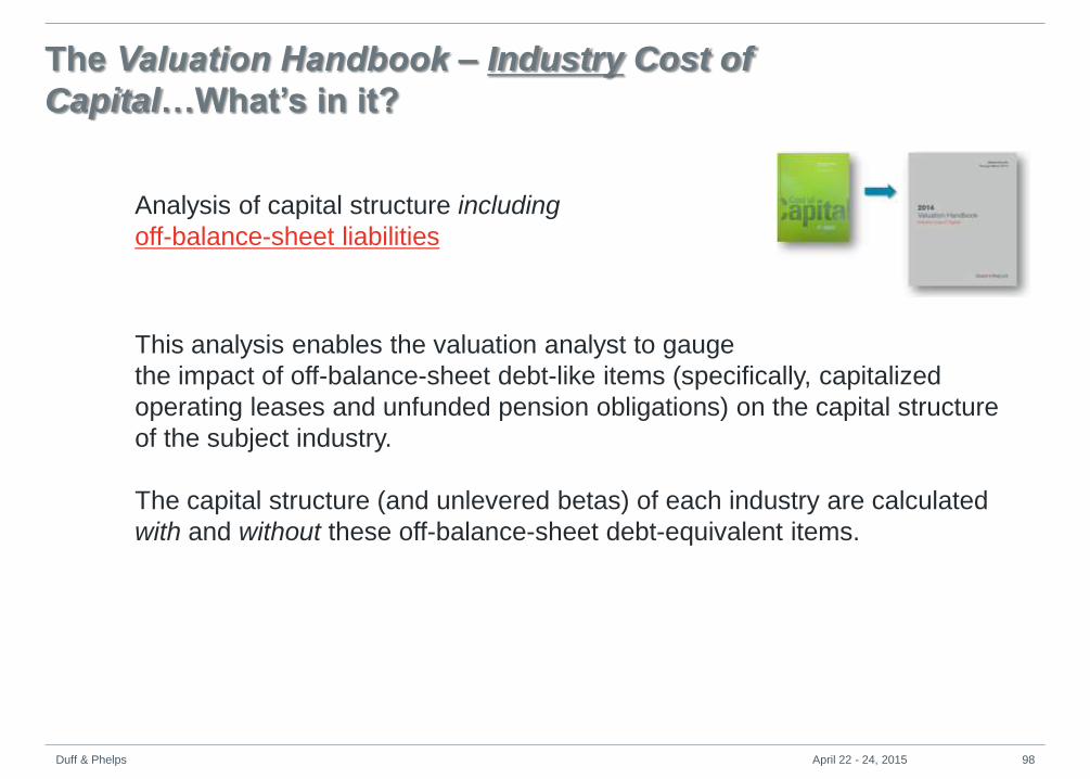
This analysis enables the valuation analyst to gauge

the impact of off-balance-sheet debt-like items (specifically, capitalized

operating leases and unfunded pension obligations) on the capital structure

of the subject industry.

The capital structure (and unlevered betas) of each industry are calculated

with and without these off-balance-sheet debt-equivalent items.

Analysis of capital structure including

off-balance-sheet liabilities




Calculated Using Book Debt

Calculated Using Book Debt +

Off-Balance-Sheet Debt

SIC Industry Description Debt-to-Total-Capital (%) Debt-to-Total-Capital (%)

57

Home Furnishings,

Furnishing, and

Equipment Stores

5.8 21.7

591Drug Stores and

Proprietary Stores13.9 27.7

3711Motor Vehicles and

Passenger Car Bodies37.0 45.8

SIC Industry Description

Primary Driver of Change

in Capital Structure

57

Home Furnishings,

Furnishing, and

Equipment Stores

Operating Leases

591Drug Stores and

Proprietary StoresOperating Leases

3711Motor Vehicles and

Passenger Car BodiesUnfunded Pension Liabilities


Country-level Cost of Capital

The annual International Valuation Handbook ‒ Guide to Cost of Capital provides

the same type of country-level analysis previously published in the

Morningstar/Ibbotson “international” cost of capital reports.

The 2014 International Valuation Handbook ‒ Guide to Cost of Capital provides

country-level country risk premia (CRPs) and country-level equity risk premia

(ERPs) which can be used to estimate country-level cost of equity capital globally

for up to 188 countries globally, from the perspective of investors based in 55

different countries.


Global Cost of Capital Models

‘‘I know how to value a business in my country, but this one is in Country X,

a developing economy. What should I use for a discount rate?’’

The risks associated with international investing can be broadly

characterized as:

• Financial

• Economic

• Political

A good understanding of cost of capital concepts is essential information

for executives making global investment decisions.


There are several common approaches to estimate an international cost of

equity capital. The following are just a few of the more commonly used

models:

1.Global CAPM (a.k.a. World CAPM model)

2.Single country version of the CAPM

3.Country or Sovereign Yield Spread model

4.Relative Volatility model

5.Erb-Harvey-Viskanta Country Credit Rating (CCR) model

Commonly Used International Cost of Equity

Capital Models


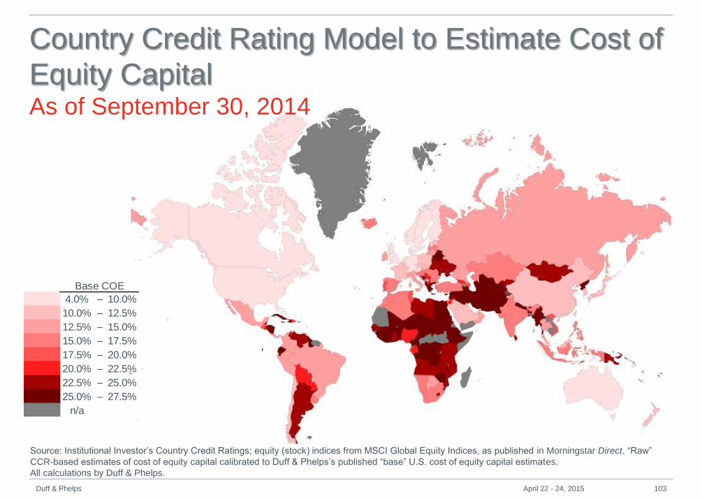
Source: Institutional Investor’s Country Credit Ratings; equity (stock) indices from MSCI Global Equity Indices, as published in Morningstar Direct. “Raw”

CCR-based estimates of cost of equity capital calibrated to Duff & Phelps’s published “base” U.S. cost of equity capital estimates.

All calculations by Duff & Phelps.

4.0% – 10.0%

10.0% – 12.5%

12.5% – 15.0%

15.0% – 17.5%

17.5% – 20.0%

20.0% – 22.5%

22.5% – 25.0%

25.0% – 27.5%

n/a

Base COE

Country Credit Rating Model to Estimate Cost of

Equity Capital As of September 30, 2014


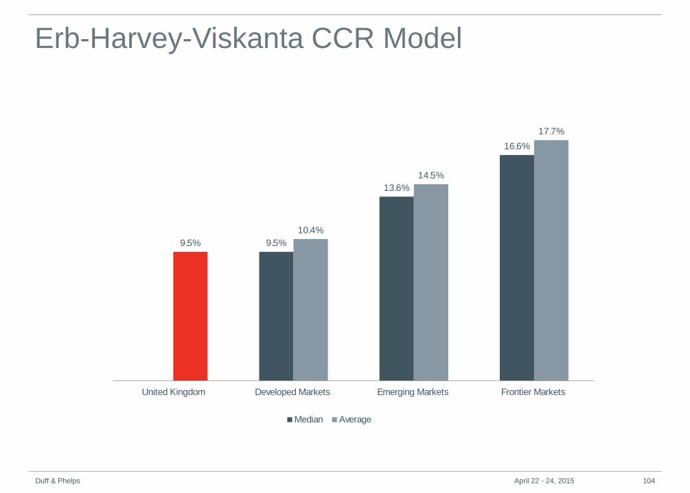
9.5%

13.6%

16.6%

9.5%

10.4%

14.5%

17.7%

United Kingdom Developed Markets Emerging Markets Frontier Markets

Median Average

Erb-Harvey-Viskanta CCR Model


7.3%

9.8%

11.8%

14.8%

21.5%

27.9%

10.3%

7.4%

9.7%

12.3%

14.8%

20.9%

28.4%

China (AA-) AAA AA A BBB BB B – SD

Median COE Based on S&P Credit Rating Average COE Based on S&P Credit Rating



8.5%

10.9%

10.2%

8.3%

9.8%

9.2%

12.9%

12.9%

13.0%

15.1%

United States

China

Japan

Germany

France

United Kingdom

Brazil

Russia

Italy

India



17.9%

9.6%

0%

2%

4%

6%

8%

10%

12%

14%

16%

18%

20%

Financial Crisis

Less Healthy Economies (Greece, Portugal, Spain)

Healthier Economies (Germany, U.K., France)



International Cost of Capital Data Sources

Credit Suisse Global Investment Returns Sourcebook and

Yearbook 2014 by Elroy Dimson, Paul Marsh, and Mike Staunton

– 21 countries

Market Risk Premium used in 88 countries in 2014: a survey with

8,228 answers by Pablo Fernandez, Palo Linares, and Isabel

Fernandez Acin

Damodaran website

Bloomberg Implied Equity Risk Model


Valuation Handbook series The upcoming 2015 International Valuation Handbook ‒ Industry Cost of Capital

will provide the same type of industry-level analysis published in the U.S.-data-

based annual Valuation Handbook ‒ Industry Cost of Capital, but for non-U.S.

companies.

Upcoming

(Fall 2015)

1 2 3 4

Company-level

data

Industry-level

data

Country-level

data

International

Industry-level

data


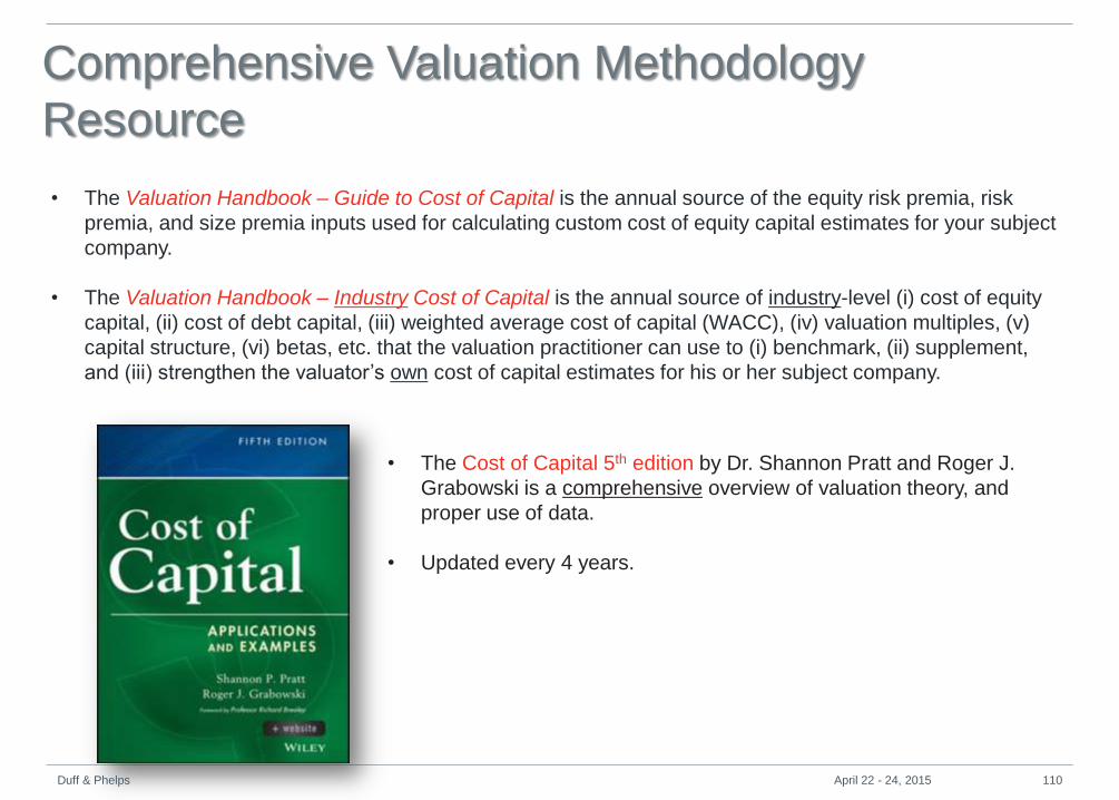
Comprehensive Valuation Methodology

Resource

• The Cost of Capital 5th edition by Dr. Shannon Pratt and Roger J.

Grabowski is a comprehensive overview of valuation theory, and

proper use of data.

• Updated every 4 years.

• The Valuation Handbook – Guide to Cost of Capital is the annual source of the equity risk premia, risk

premia, and size premia inputs used for calculating custom cost of equity capital estimates for your subject

company.

• The Valuation Handbook – Industry Cost of Capital is the annual source of industry-level (i) cost of equity

capital, (ii) cost of debt capital, (iii) weighted average cost of capital (WACC), (iv) valuation multiples, (v)

capital structure, (vi) betas, etc. that the valuation practitioner can use to (i) benchmark, (ii) supplement,

and (iii) strengthen the valuator’s own cost of capital estimates for his or her subject company.


About Duff &Phelps


Duff & Phelps

Dedicated to Delivering Value


Global Presence

More Than 70 Offices Worldwide


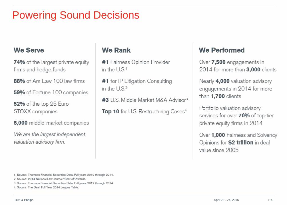
Powering Sound Decisions


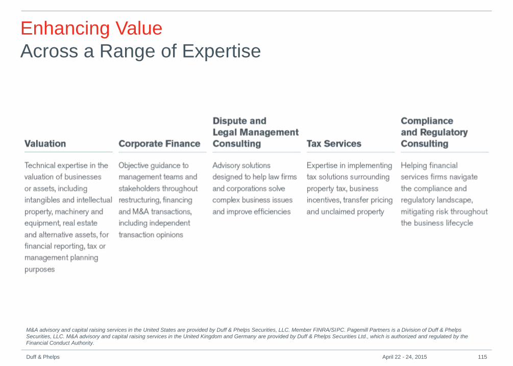
M&A advisory and capital raising services in the United States are provided by Duff & Phelps Securities, LLC. Member FINRA/SIPC. Pagemill Partners is a Division of Duff & Phelps

Securities, LLC. M&A advisory and capital raising services in the United Kingdom and Germany are provided by Duff & Phelps Securities Ltd., which is authorized and regulated by the

Financial Conduct Authority.

Enhancing Value

Across a Range of Expertise


Our Services


Services Across the Transaction Lifecycle


Regulatory Affiliations


Industry Expertise

Serving Nearly 60% of Fortune 100 Companies


Date post:	15-Mar-2018
Category:	Documents
Upload:	phunghanh
View:	215 times
Download:	1 times

presented by: Roger J. Grabowski, · PDF filepresented by: Roger J. Grabowski, FASA - 24, 2015...

Documents