PRESSURE BROADENING AND PRESSURE SHIFT OF DIATOMIC IODINE AT 675 NM by ERICH N. WOLF A DISSERTATION Presented to the Department of Chemistry and the Graduate School of the University of Oregon in partial fulfillment of the requirements for the degree of Doctor of Philosophy June 2009
Transcript
PRESSURE BROADENING AND PRESSURE SHIFT
OF DIATOMIC IODINE AT 675 NM
by
ERICH N. WOLF
A DISSERTATION
Presented to the Department of Chemistry and the Graduate School of the University of Oregon
in partial fulfillment of the requirements for the degree of
Doctor of Philosophy
June 2009
ii
Erich N. Wolf / Pressure Broadening and Pressure Shift of I2 at 675 nm / June 2009
“Pressure Broadening and Pressure Shift of Diatomic Iodine at 675 nm,” a dissertation
prepared by Erich N. Wolf in partial fulfillment of the requirements for the Doctor of
Philosophy degree in the Department of Chemistry. This dissertation has been
approved and accepted by:
____________________________________________________________ Dr. David Herrick, Chair of the Examining Committee ________________________________________ Date Committee in Charge: Dr. David R. Herrick, Chair Dr. John L. Hardwick Dr. Michael G. Raymer Dr. Jeffrey A. Cina Dr. David R. Tyler Accepted by: ____________________________________________________________ Dean of the Graduate School
iii
Erich N. Wolf / Pressure Broadening and Pressure Shift of I2 at 675 nm / June 2009
An Abstract of the Dissertation of Erich N. Wolf for the degree of Doctor of Philosophy in the Department of Chemistry to be taken June 2009 Title: PRESSURE BROADENING AND PRESSURE SHIFT OF DIATOMIC
Dr. David Herrick, Chair of the Examining Committee
Doppler-limited, steady-state, linear absorption spectra of 127I2 (diatomic iodine)
near 675 nm were recorded with an internally-referenced wavelength modulation
spectrometer, built around a free-running diode laser using phase-sensitive detection,
and capable of exceeding the signal-to-noise limit imposed by the 12-bit data acquisition
system. Observed I2 lines were accounted for by published spectroscopic constants.
Pressure broadening and pressure shift coefficients were determined respectively
from the line-widths and line-center shifts as a function of buffer gas pressure, which
were determined from nonlinear regression analysis of observed line shapes against a
Gaussian-Lorentzian convolution line shape model. This model included a linear
superposition of the I2 hyperfine structure based on changes in the nuclear electric
quadrupole coupling constant. Room temperature (292 K) values of these coefficients
were determined for six unblended I2 lines in the region 14,817.95 to 14,819.45 cm−1 for
iv
Erich N. Wolf / Pressure Broadening and Pressure Shift of I2 at 675 nm / June 2009
each of the following buffer gases: the atoms He, Ne, Ar, Kr, and Xe; and the molecules
H2, D2, N2, CO2, N2O, air, and H2O. These coefficients were also determined at one
additional temperature (388 K) for He and CO2, and at two additional temperatures (348
and 388 K) for Ar. Elastic collision cross-sections were determined for all pressure
broadening coefficients in this region. Room temperature values of these coefficients
were also determined for several low-J I2 lines in the region 14,946.17 to 14,850.29
cm−1 for Ar.
A line shape model, obtained from a first-order perturbation solution of the
time-dependent Schrödinger equation for randomly occurring interactions between a
two-level system and a buffer gas treated as step-function potentials, reveals a
relationship between the ratio of pressure broadening to pressure shift coefficients and
a change in the wave function phase-factor, interpreted as reflecting the “cause and
effect” of state-changing events in the microscopic domain. Collision cross-sections
determined from this model are interpreted as reflecting the inelastic nature of
collision-induced state-changing events.
A steady-state kinetic model for the two-level system compatible with the
Beer-Lambert law reveals thermodynamic constraints on the ensemble-average state-
changing rates and collision cross-sections, and leads to the proposal of a relationship
between observed asymmetric line shapes and irreversibility in the microscopic
domain.
(The graduate school at the University of Oregon imposes a word limit [350
words] on dissertation abstracts so that the last paragraph of the abstract did not include
v
Erich N. Wolf / Pressure Broadening and Pressure Shift of I2 at 675 nm / June 2009
a passage akin to the following: A modified version of the Einstein A and B Coefficient
model appropriate for linear absorption is offered [Section 2.11], one that is based on the
mathematical operation of convolutions and allows for a derivation of the Beer-Lambert
Law for the state-changing processes in the two-level model [stimulated absorption,
stimulated emission, and spontaneous emission] for the case of steady-state dynamics in
the microscopic domain. This model indicates that the rates for stimulated absorption
and stimulated emission are not necessarily equal, which is tantamount to the B
coefficients for stimulated absorption and stimulated emission not necessarily being
equal. Furthermore, this model indicates that the collision cross-sections for stimulated
absorption and stimulated emission are not equal. As well, with regard to the well
documented appearance of asymmetric line shapes in high-resolution linear absorption
spectra, it would have been mentioned that such features may be more fully consistent
with the reality that the universe we live in [i.e. that there is no such thing as a perfectly
isolated object] is more properly described by non-Hermitian Hamiltonians; in the
context of the [non-degenerate] two-level model, the Hamiltonian that describes photon
absorption is not the Hermitian conjugate of the Hamiltonian that describes photon
emission.
Apart from the foregoing addendum to the abstract, the inclusion of a footer on
all pages of the dissertation indicating the author’s name, dissertation title, and year of
submission of the dissertation, and inclusion of publications in the field of
organometallic chemistry, this version of the dissertation is the one that was accepted by
the graduate school at the University of Oregon.)
vi
Erich N. Wolf / Pressure Broadening and Pressure Shift of I2 at 675 nm / June 2009
CURRICULUM VITAE NAME OF AUTHOR: Erich N. Wolf GRADUATE AND UNDERGRADUATE SCHOOLS ATTENDED: University of Oregon California State University, Northridge DEGREES AWARDED: Doctor of Philosophy in Chemistry, 2009, University of Oregon Bachelor of Science in Physics, 1993, California State University, Northridge AREAS OF SPECIAL INTEREST: Chemical Physics, Quantum Electrodynamics, Statistical Physics, Thermodynamics, Solid State Physics, Classical Physics, Astrophysics and Cosmology, and Mathematics Atomic and Molecular Spectroscopy Inorganic and Organometallic Chemistry and Catalysis Materials and Properties of Materials PROFESSIONAL EXPERIENCE: Research Assistant, Department of Chemistry, University of Oregon, Eugene, June 2001 − September 2007 Teaching Assistant, Undergraduate Physical Chemistry Laboratory, Department of Chemistry, University of Oregon, Eugene, September 2001 − June 2002, September 2003 − June 2004, and September 2005 − June 2006 Research Assistant, Department of Chemistry, California State University, Northridge, March 1988 − June 1992
vii
Erich N. Wolf / Pressure Broadening and Pressure Shift of I2 at 675 nm / June 2009
PUBLICATIONS:
Spectroscopy: Arteaga, S. W., C. M. Bejger, J. L. Gerecke, J. L. Hardwick, Z. T. Martin, J. Mayo, E. A. McIlhattan, J.-M. F. Moreau, M. J. Pilkenton, M. J. Polston, B. T. Robertson, and E. N. Wolf. “Line Broadening and Shift Coefficients of Acetylene at 1550 nm.” Journal of Molecular Spectroscopy 243 (2007): 253-266. Hardwick, J. L., Z. T. Martin, M. J. Pilkenton, and E. N. Wolf. “Diode Laser Absorption Spectra of H12C13CD and H13C12CD at 6500 cm−1.” Journal of Molecular Spectroscopy 243 (2007): 10-15. Hardwick, J. L., Z. T. Martin, E. A. Schoene, V. Tyng, and E. N. Wolf. “Diode Laser Absorption Spectrum of Cold Bands of C2HD at 6500 cm−1.” Journal of Molecular Spectroscopy 239 (2006): 208-215. Eng, J. A., J. L. Hardwick, J. A. Raasch, and E. N. Wolf. “Diode Laser Wavelength Modulated Spectroscopy of I2 at 675 nm.” Spectrochimica Acta Part A 60 (2004): 3413-3419.
Organometallic Chemistry: Rosenberg E., S. E. Kabir, L. Milone, R. Gobetto, D. Osella, M. Ravera, T. McPhillips, M. W. Day, D. Carlot, S. Hajela, E. Wolf, K. I. Hardcastle. “Comparative Reactivity of Triruthenium and Triosmium μ 3-η 2-Imidoyls. 2. Reactions with Alkynes.” Organometallics 16 (1997): 2674-2681. Rosenberg E., L. Milone, R. Gobetto, D. Osella, K. I. Hardcastle, S. Hajela, K. Moizeau, M. Day, E. Wolf, D. Espitia. “Comparative Reactivity of Triruthenium and Triosmium μ 3-η 2-Imidoyls. 1. Dynamics and Reactions with Carbon Monoxide, Phosphine, and Isocyanide.” Organometallics 16 (1997): 2665-2673. Rosenberg E., S. E. Kabir, M. Day, K. I. Hardcastle, E. Wolf, T. McPhillips. “Chemistry of Nitrogen Donors with μ 3-Imidoyl Triosmium Clusters: Dynamics of a Monometallic Site in a Trimetallic Cluster.” Organometallics 14 (1995): 721-733.
viii
Erich N. Wolf / Pressure Broadening and Pressure Shift of I2 at 675 nm / June 2009
Rosenberg E., M. Day, W. Freeman, K. I. Hardcastle, M. Isomaki, S. E. Kabir, T. McPhillips, L. G. Scott, E. Wolf; “Comparative study of the reactions of diazomethane with μ 3-imidoyl and μ 3-butyne trinuclear clusters”, Organometallics 11 (1992): 3376-3384. Rosenberg E., M. W. Day, S. Hajela, S. E. Kabir, M. Irving, T. McPhillips, E. Wolf, K. I. Hardcastle, L. Milone, et al.; “Reactions of tertiary amines with trinuclear clusters. 3. Reactions of N-methylpyrrolidine with Ru3(CO)12 and Os3(CO)10(CH3CN)2.” Organometallics 10 (1991): 2743-2751. Rosenberg E., S. E. Kabir, K. I. Hardcastle, M. Day, E. Wolf; “Reactions of secondary amines with triosmium decacarbonyl bis(acetonitrile): room-temperature carbon-hydrogen bond activation and transalkylation.” Organometallics 9 (1990): 2214-2217.
ix
Erich N. Wolf / Pressure Broadening and Pressure Shift of I2 at 675 nm / June 2009
ACKNOWLEDGMENTS
Thomas Dyke for research opportunity, academic guidance, and financial
assistance.
John Hardwick for research opportunity and academic guidance.
David Herrick, Jeffrey Cina and Michael Raymer for academic guidance.
Finally, and most importantly, Vivian Ding, without whom this
dissertation would not be possible.
x
Erich N. Wolf / Pressure Broadening and Pressure Shift of I2 at 675 nm / June 2009
I bow to all the high and holy lamas.
xi
Erich N. Wolf / Pressure Broadening and Pressure Shift of I2 at 675 nm / June 2009
TABLE OF CONTENTS
Chapter Page
I. INTRODUCTION 1 − CONTEXT AND OVERVIEW ................................ 11.1 Overview of Chapter I ............................................................................ 11.2 Historical Overview of Absorption Spectroscopy .................................. 11.3 Linear Absorption Spectroscopy ............................................................ 51.4 Wavelength Modulated Linear Absorption Spectroscopy ..................... 71.5 Research and Education ......................................................................... 81.6 Error Propagation of Uncorrelated Parameters ...................................... 101.7 Endnotes for Chapter 1 ........................................................................... 11
II. INTRODUCTION 2 − BACKGROUND KNOWLEDGE .......................... 13
2.1 Overview of Chapter II ........................................................................... 132.2 Electronic States, Hund’s Coupling, and Selection Rules ...................... 132.3 Spectroscopic Constants ......................................................................... 172.4 Line Intensities in Vibronic Bands ......................................................... 18
2.5 Nuclear Hyperfine Structure ................................................................... 292.6 Nuclear Hyperfine Structure of Diatomic Iodine ................................... 322.7 Frequency and Time in Spectroscopy .................................................... 342.8 Line-Shape Model for Steady-State Frequency Domain Spectra ........... 352.9 The Two-Level System Model ............................................................... 392.10 The Four-Level System Model ............................................................. 422.11 Steady-State Kinetic Model .................................................................. 442.12 Collision Processes ............................................................................... 612.13 Pressure Broadening and Pressure Shift Coefficients .......................... 622.14 The Hermitian Hamiltonian .................................................................. 65
xii
Erich N. Wolf / Pressure Broadening and Pressure Shift of I2 at 675 nm / June 2009
Chapter Page
2.15 Endnotes for Chapter 2 ....................................................................... 68
III. DATA COLLECTION ................................................................................ 763.1 Overview of Chapter III ....................................................................... 763.2 Internally Referenced Absorption Spectrometer .................................. 77
3.2.1 Philips CQL806/30 Laser Diode System Spectrometer .............. 793.2.2 Collimation with an Off-Axis Parabolic Reflector ...................... 903.2.3 New Focus 6202 External Cavity Laser Diode System .............. 933.2.4 Signal-to-Noise Ratios, Modulation Depths,
and Laser Line Widths ................................................................ 973.3 Reference and Sample Gas Cells .......................................................... 101
3.3.1 Design and Construction of Gas Cells ......................................... 1023.3.2 Preparation and Handling of Gas Cells ....................................... 1033.3.3 Heating the Sample Gas Cell ....................................................... 106
3.4 Endnotes for Chapter 3 ......................................................................... 109
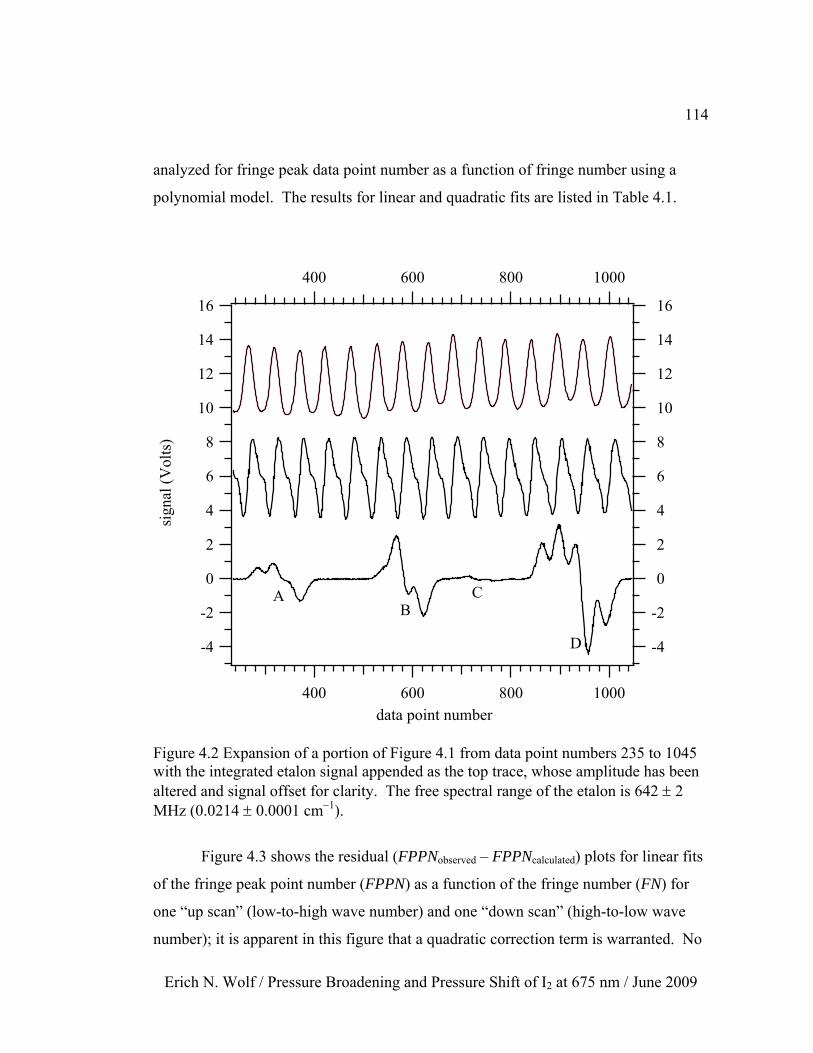
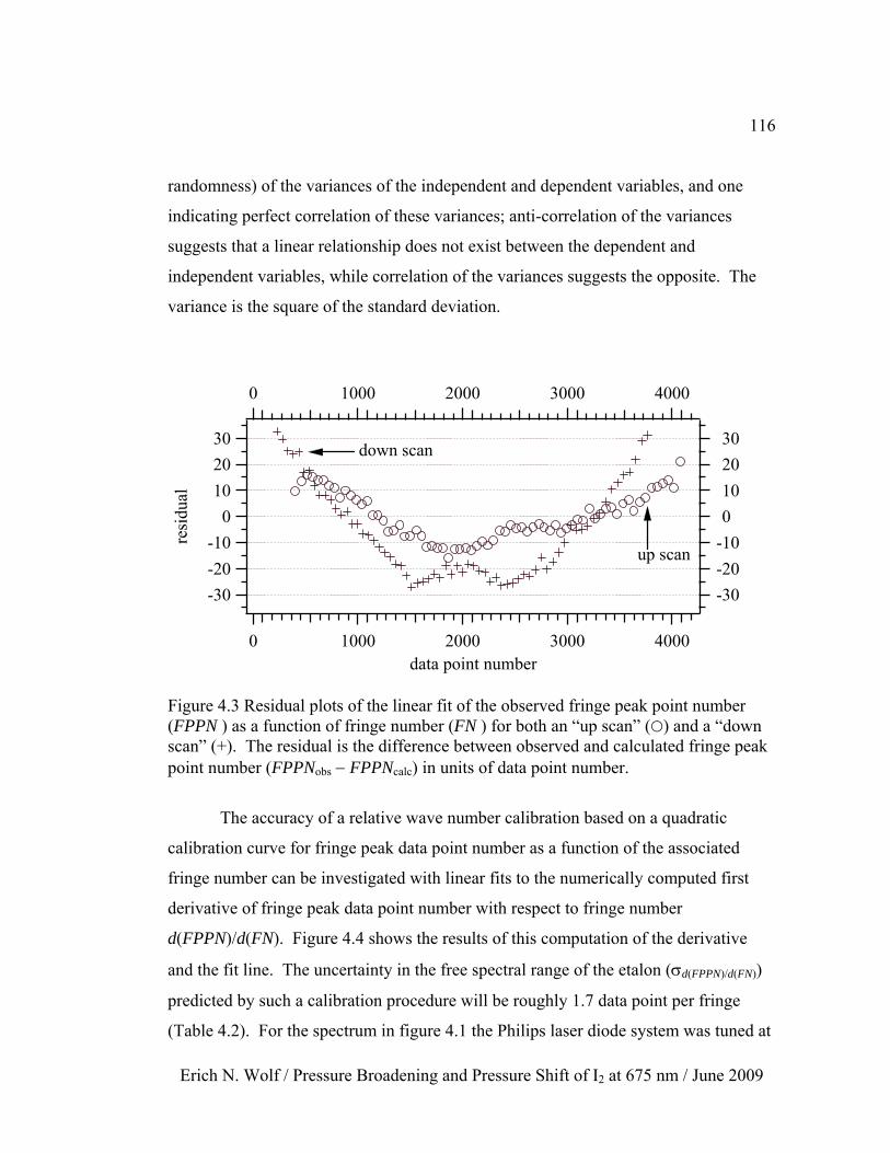
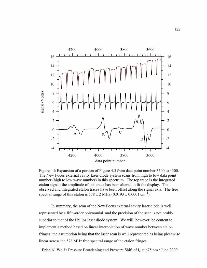
IV. ANALYSIS 1 − ASSIGNMENT AND CALIBRATION .......................... 1114.1 Overview of Chapter IV ....................................................................... 1114.2 Linearity of Philips Laser Diode System Scans ................................... 1124.3 Linearity of New Focus External Cavity Laser Diode System Scans .. 1204.4 Etalon Fringe Widths ............................................................................ 1244.5 Assignment of Diatomic Iodine Spectral Features ............................... 126
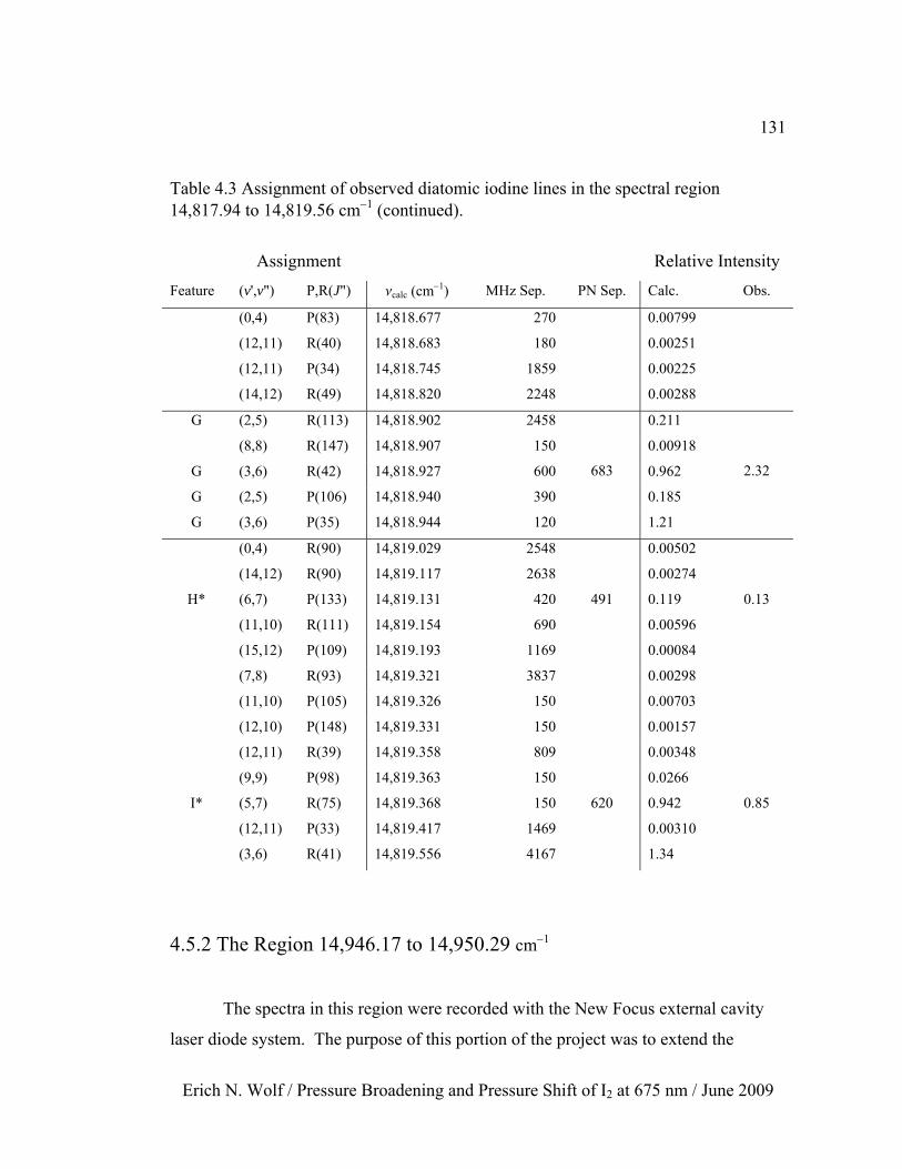
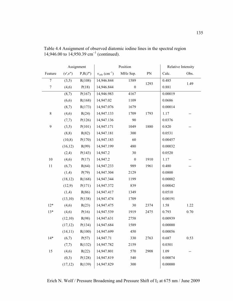
4.5.1 The Region 14,817.95 to 14,819.45 cm−1 .................................... 1284.5.2 The Region 14,946.17 to 14,950.29 cm−1 .................................... 131
4.6 Wave Number Calibration of Diatomic Iodine Spectra ....................... 1394.6.1 Two Diatomic Iodine Features .................................................... 1404.6.2 Many Diatomic Iodine-Features and Etalon Fringes ................... 1424.6.3 Comparison of Etalon and Polynomial Calibration Methods ...... 146
4.7 Endnotes for Chapter 4 ......................................................................... 147
xiii
Erich N. Wolf / Pressure Broadening and Pressure Shift of I2 at 675 nm / June 2009
Chapter Page
V. ANALYSIS 2 − LINE SHAPE ANALYSIS ................................................ 1495.1 Overview of Chapter V .......................................................................... 1495.2 Line Shape Components and the Convolution Model ............................ 1505.3 Linear Absorption and Line Shape ......................................................... 1545.4 Diatomic Iodine Line Shape with Nuclear Hyperfine Structure ............ 157
5.4.1 Model for High-J Lines ................................................................. 1585.4.2 Models for Low-J Lines ................................................................ 162
5.5 Voigt Line Shape and Nonlinear Fitting ................................................ 1645.6 Wavelength Modulation and De-Modulation ......................................... 1695.7 Effects of Neighboring Lines on Shape and Position ............................. 1735.8 Some Fit Results and Comparisons ........................................................ 175
5.8.1 A Single Diatomic Iodine Feature ................................................. 1765.8.2 The Spectral Region 14,817.95 to 14,819.45 cm−1 ....................... 1845.8.3 Nonlinear Pressure Shift Coefficient ............................................. 193
5.9 Endnotes for Chapter 5 ........................................................................... 194
VI. RESULTS 1 − COEFFICIENTS AND CROSS-SECTIONS ..................... 197
6.1 Overview of Chapter VI ....................................................................... 1976.2 Pressure Broadening and Pressure Shift Coefficients .......................... 199
6.2.1 Atomic Buffer Gases at Room Temperature (292 K) ................. 2006.2.2 Molecular Buffer Gases at Room Temperature (292 K) ............. 2056.2.3 Multiple Temperatures (292, 348, and 388 K) ............................ 209
6.3 Collision Cross-Sections ...................................................................... 2126.3.1 Time-resolved vs. Frequency Domain Spectroscopic Methods .. 219
6.4 Endnotes for Chapter 6 ......................................................................... 222
VII. RESULTS 2 − TIME-DEPENDENT QUANTUM MECHANICS .......... 223
7.1 Overview of Chapter VII .................................................................... 2237.2 The Two-Level System Hamiltonian ................................................. 2247.3 Time-Dependent First-Order Perturbation Theory ............................. 2307.4 Excited-State Probabilities ................................................................. 239
xiv
Erich N. Wolf / Pressure Broadening and Pressure Shift of I2 at 675 nm / June 2009
Chapter Page
7.5 Pressure Broadening and Pressure Shift Coefficients ........................ 2427.6 Asymmetric Line Shape ..................................................................... 2487.7 Non-Hermitian Hamiltonians ............................................................. 2537.8 Endnotes for Chapter VII ................................................................... 258
VIII. SUMMARY AND CONCLUSIONS ....................................................... 260
8.1 Summary and Conclusions ................................................................. 2608.2 Endnotes for Chapter VIII .................................................................. 266
Erich N. Wolf / Pressure Broadening and Pressure Shift of I2 at 675 nm / June 2009
LIST OF FIGURES
Figure Page
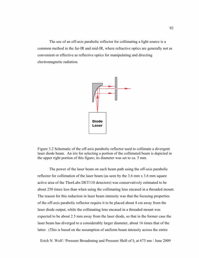
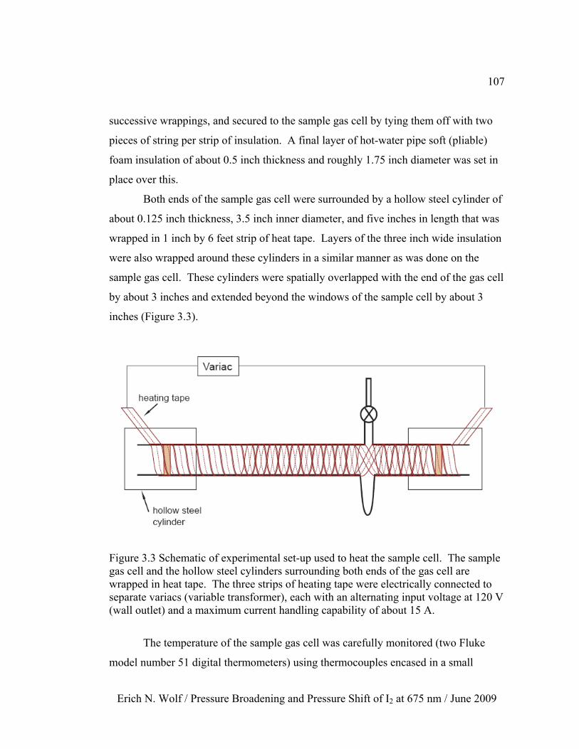
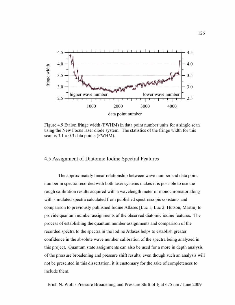
1.1 Depiction of Newton’s experiments with prisms ....................................... 2 1.2 Solar spectrum at optical wavelengths ....................................................... 3 2.1 Potential energy surfaces for the X and B electronic states of I2 ............... 16 2.2 Simulation of the relative intensities of the vibration levels ...................... 20 2.3 Simulation of the relative intensities of a rotational progression ............... 21 2.4 Franck-Condon factors for B−X transitions in I2 ....................................... 27 2.5 The two-level system model ....................................................................... 40 2.6 The four-level system model depicting phase-changing state-changes ..... 42 2.7 The four-level system model ...................................................................... 43 2.8 Ensemble-average state-changes in the time domain ................................. 57 3.1 Schematic of the internally referenced absorption spectrometer ............... 78 3.2 Schematic of the off-axis parabolic reflector ............................................. 92 3.3 Schematic of experimental set-up used to heat the sample cell ................. 107 4.1 Wavelength-modulated spectrum, Philips laser diode system ................... 113 4.2 Expansion of a portion of Figure 4.1 .......................................................... 114 4.3 Residual plots of the linear fit of FPPN as a function of FN ..................... 116 4.4 Numerical first derivative of FPPN with respect to FN ............................. 118 4.5 Wavelength-modulated spectrum, New Focus laser diode system ............ 121 4.6 Expansion of a portion of Figure 4.5 .......................................................... 122 4.7 Residual plots of the fits of FPPN as a function of FN .............................. 123 4.8 Etalon fringe width (FWHM) for the Philips laser diode system ............... 125 4.9 Etalon fringe width (FWHM) for the New Focus laser diode system ........ 126 4.10 I2 spectrum for the region 14,817.95 to 14,819.45 cm−1 ........................... 129 4.11 Spectrum of I2 for the region 14,946.17 to 14,948.43 cm−1 ..................... 132 4.12 Spectrum of I2 for the region 14,948.08 to 14,950.29 cm−1 ..................... 133 4.13 Calibration residuals of I2 feature wave number positions ....................... 144 4.14 Difference in wave number positions for two calibration methods ......... 147
xvi
Erich N. Wolf / Pressure Broadening and Pressure Shift of I2 at 675 nm / June 2009
Figure Page
5.1 Convolution of distributions to form a Voigt distribution .......................... 153 5.2 Simulation of direct linear absorption spectrum of I2 ................................ 160 5.3 Simulation of wavelength-modulated spectrum of I2 ................................. 161 5.4 Residuals of fits to Voigt distributions using Humlíček approximation .... 167 5.5 Simulations of wavelength-modulated phase-sensitive detection .............. 171 5.6 Observed and calculated I2 Feature A at seven argon pressure .................. 177 5.7 Comparison of fit results for I2 Feature A with argon ................................ 180 5.8 Comparison of the average DeQq in the hyperfine structure of I2 ............. 187 5.9 Pressure broadening and pressure shift for I2 with argon ........................... 191 6.1 Pressure broadening (Bp) and pressure shift (Sp) of I2 with noble atoms ... 203 6.2 Pressure broadening (Bp) and pressure shift (Sp) of I2 with argon .............. 205 6.3 Pressure broadening (Bp) and pressure shift (Sp) of I2 with molecules ....... 209 7.1 Collision-induced perturbations of a two-level system .............................. 229 7.2 Plot of the pressure coefficients ratio Rbs = Bp/Sp = 2tan(Da/2) ................. 245 7.3 Collision cross-sections and changes in wave function phase-factor ......... 247 A.1 Circuit diagram of the (not necessarily unity gain) summing amplifier .... 268 A.2 Circuit diagram of the (unity gain) summing amplifier ............................ 269
xvii
Erich N. Wolf / Pressure Broadening and Pressure Shift of I2 at 675 nm / June 2009
LIST OF TABLES
Table Page
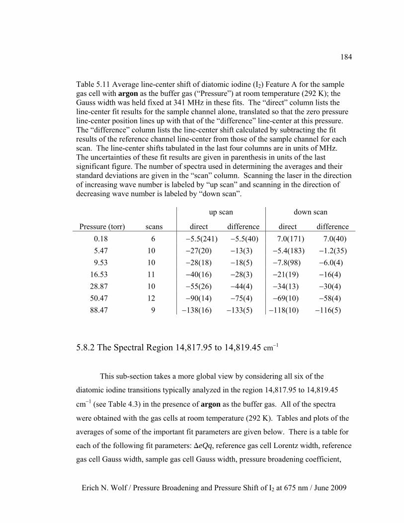
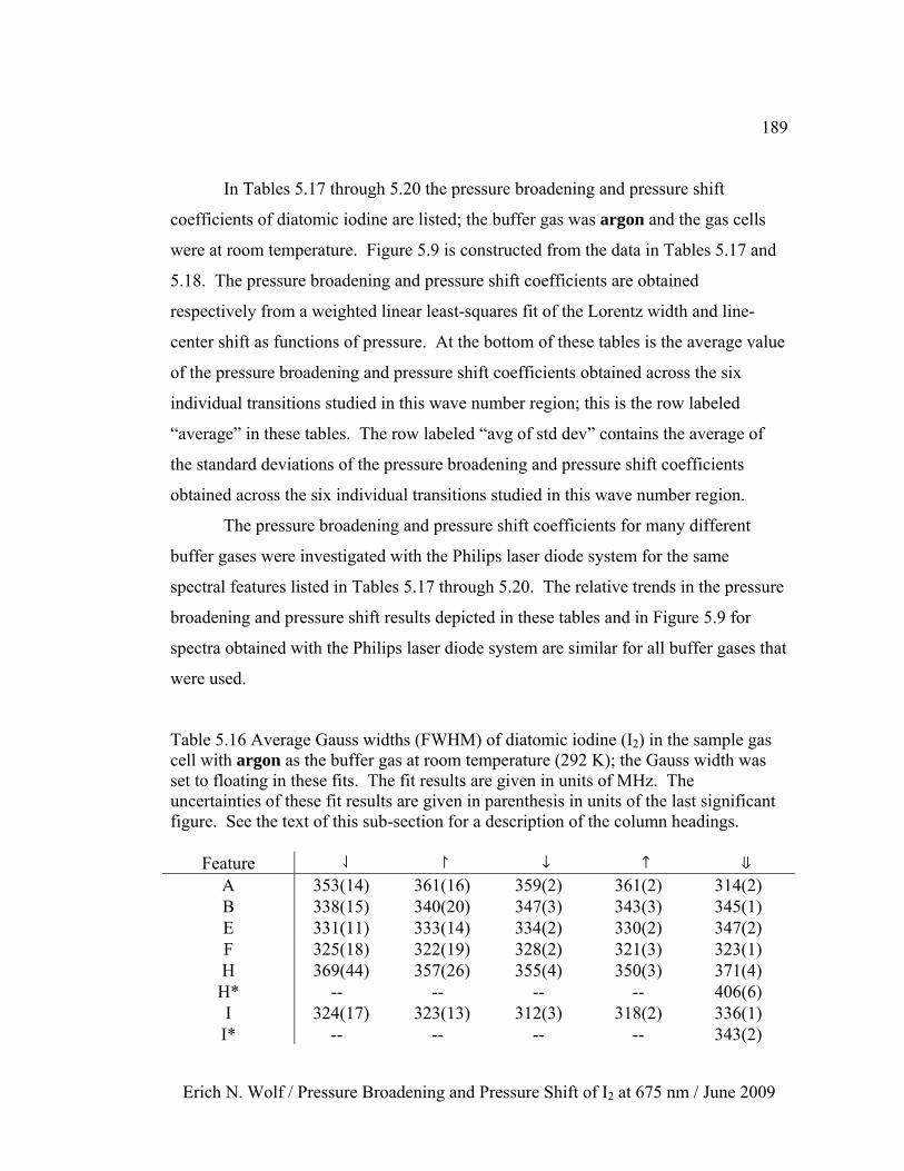
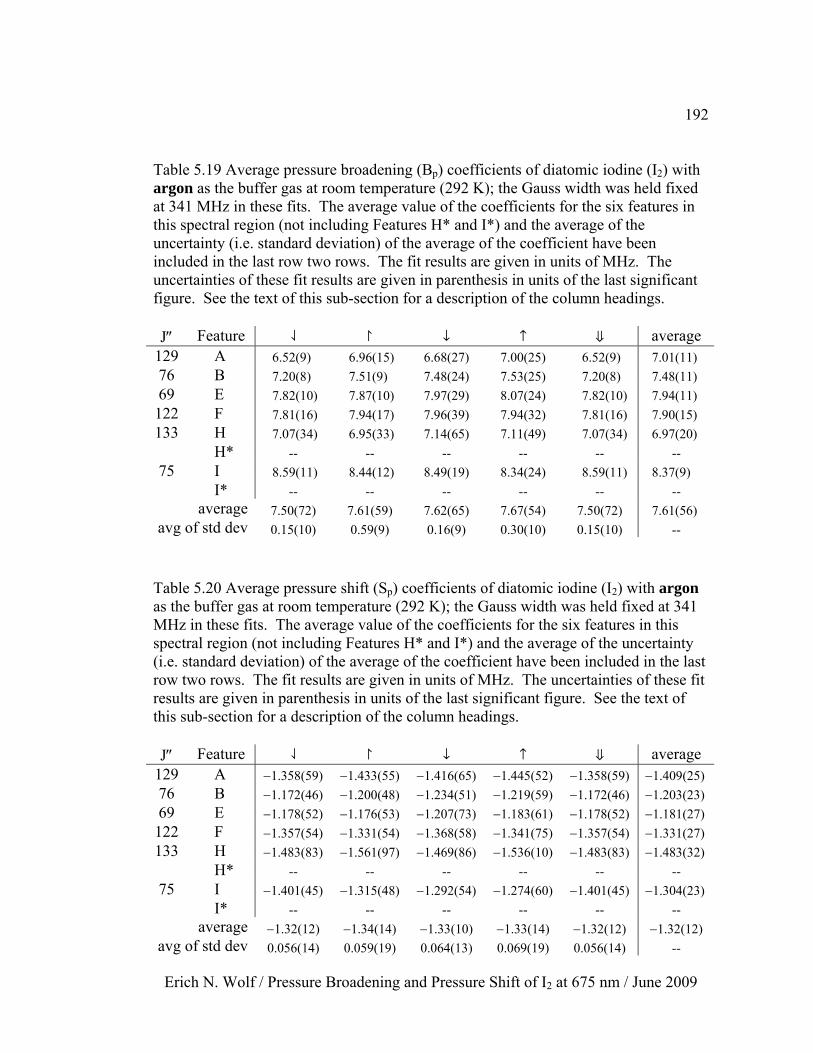
3.1 Signal-to-noise ratios of the internally-referenced spectrometer ............... 99 4.1 Fit results for FPPN as a function of FN .................................................... 115 4.2 Fit results for first derivative of FPPN with respect to FN ........................ 117 4.3 Assignment of I2 lines in the region 14,817.94 to 14,819.56 cm−1 ............ 130 4.4 Assignment of I2 lines in the region 14,946.00 to 14,950.39 cm−1 ............ 134 4.5 Linear calibration using two diatomic iodine features ............................... 141 4.6 Wave number calibration statistics for the two laser diode systems .......... 145 5.1 I2 nuclear hyperfine structure for J t 20 .................................................... 159 5.2 Fits to simulated Voigt line shapes using the Humlíček approximation .... 168 5.3 Wavelength-modulated simulations and nonlinear regression results ....... 170 5.4 Simulated line shape for range of modulation depths ................................ 172 5.5 Simulated changes in pressure coefficients of I2 ........................................ 174 5.6 Nonlinear regression fit results for the spectra of I2 Feature A .................. 179 5.7 Relative error in observed and model I2 line shape .................................... 179 5.8 Lorentz widths of I2 Feature A with argon; Gauss width floating ............. 181 5.9 Line-center shift of I2 Feature A with argon; Gauss width floating ........... 182 5.10 Lorentz widths of I2 Feature A with argon; Gauss width fixed ................ 183 5.11 Line-center shift of I2 Feature A with argon; Gauss width fixed ............. 184 5.12 Prominent spectral features of I2; 14,817.95 to 14,819.45 cm−1 .............. 186 5.13 Average DeQq in the hyperfine structure of I2; Gauss width floating....... 187 5.14 Lorentz widths of I2 in reference gas cell; Gauss width floating ............. 188 5.15 Gauss widths of I2 in reference gas cell; Gauss width floating ................ 188 5.16 Gauss widths of I2 in sample gas cell; Gauss width floating .................... 189 5.17 Pressure broadening (BP) of I2 with argon; Gauss width floating ............ 190 5.18 Pressure shift (SP) of I2 with argon; Gauss width floating ........................ 190 5.19 Pressure broadening (BP) of I2 with argon; Gauss width fixed ................. 192 5.20 Pressure shift (SP) of I2 with argon; Gauss width fixed ............................ 192
xviii
Erich N. Wolf / Pressure Broadening and Pressure Shift of I2 at 675 nm / June 2009
Table Page
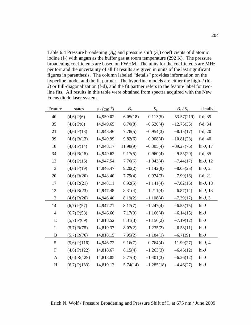
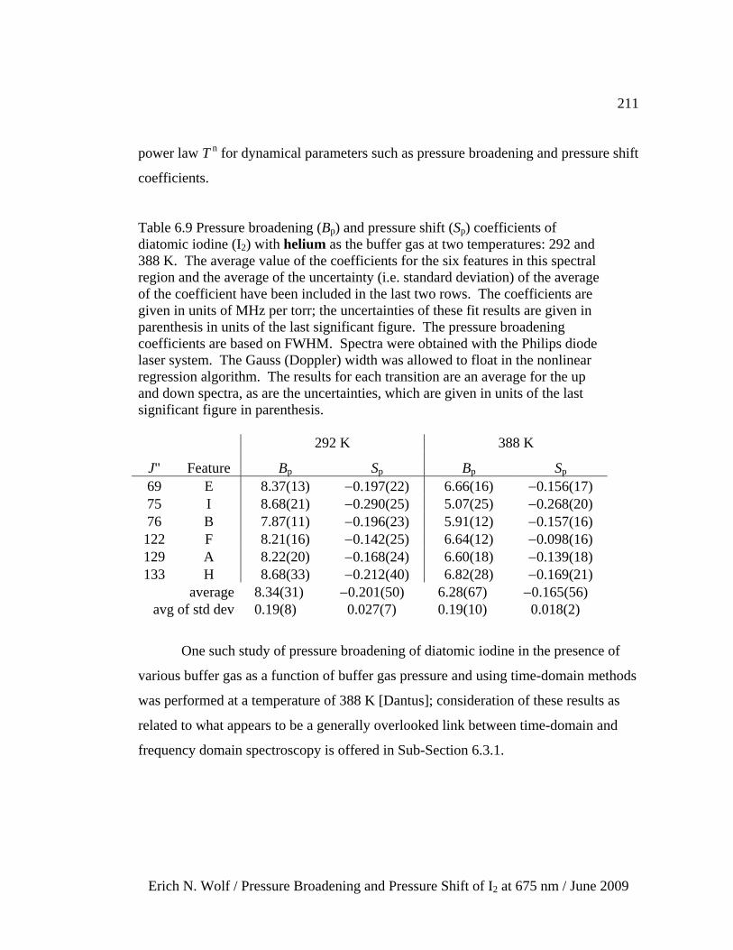
6.1 Prominent spectral features of I2; 14,817.95 to 14,819.45 cm−1 ................ 198 6.2 Pressure broadening (Bp) of I2 with noble atoms ........................................ 201 6.3 Pressure shift (Sp) of I2 with noble atoms ................................................... 202 6.4 Pressure broadening (Bp) and pressure shift (Sp) of I2 with argon .............. 204 6.5 Pressure broadening (Bp) and pressure shift (Sp) of I2 with air and water .. 206 6.6 Pressure broadening (Bp) of I2 with molecules ........................................... 207 6.7 Pressure shift (Sp) of I2 with molecules ...................................................... 208 6.8 Bp and Sp of I2 with argon at 292, 348, and 388 K ..................................... 210 6.9 Bp and Sp of I2 with helium at 292 and 388 K ............................................ 211 6.10 Bp and Sp of I2 with carbon dioxide 292 and 388 K .................................. 212 6.11 Collision cross-section of I2 with noble atoms ......................................... 216 6.12 Collision cross-section of I2 with molecules ............................................ 217 6.13 Collision cross-section of I2 with argon at 292, 348, and 388 K .............. 218 6.14 Collision cross-section of I2 with helium and carbon dioxide .................. 218 6.15 Time domain versus frequency domain collision cross-sections ............. 220 7.1 Change in the wave function phase-factor of I2 with noble gases .............. 246
1
Erich N. Wolf / Pressure Broadening and Pressure Shift of I2 at 675 nm / June 2009
CHAPTER I
INTRODUCTION 1 − CONTEXT AND OVERVIEW
1.1 Overview of Chapter I
This chapter begins with a brief historical review of linear absorption
spectroscopy, which seeks to provide a context for the measurement of pressure
broadening and pressure shift coefficients. A brief overview of the experimental
methods of linear absorption spectroscopy and wavelength-modulated linear
absorption spectroscopy are presented. The role of such methods in training the next
generation of scientists is briefly explored. The last section on error propagation is
essential in the attempt to make this manuscript more complete and self-contained.
1.2 Historical Overview of Absorption Spectroscopy
In the mid-17th century, Newton constructed a low resolution spectrometer
using a glass prism, which he then used to investigate the properties of the light
emitted by the sun (Figure 1.1). Passing sunlight through a single prism, Newton
observed the (spatial) dispersion of white light into an ordered band of colors, the
same progression observed in rainbows for time immemorial. Newton also reported
on the reversibility (at the macroscopic level) of this dispersion process by using a
second prism to recombine the light dispersed by the first prism to form a beam of
white light.
2
Erich N. Wolf / Pressure Broadening and Pressure Shift of I2 at 675 nm / June 2009
Figure 1.1 Depiction of Newton’s experiments of dispersing (decomposing) sunlight into its constituent colors using a glass prism. (Digitized images from Voltaire's Elements de la Philosophie de Newton, published in 1738.)
Roughly 150 years later the design and construction of spectrometers had
improved in (wavelength) resolution and (detection) sensitivity so that discrete
absorption features (a.k.a. lines) in the spectrum of the sun were revealed (Figure 1.2).
The introduction of the diffraction grating for light dispersion was the source of these
3
Erich N. Wolf / Pressure Broadening and Pressure Shift of I2 at 675 nm / June 2009
improvements. As well, spectrometers were constructed for observing the emission
spectra of burning samples (i.e. a relatively fast reduction-oxidation reaction), which
also revealed the existence of discrete spectral features, or lines. It was eventually
recognized that the features observed in absorption and emission spectra are related to
each other, that the dark lines of an absorption spectrum occur at the same wavelength
as the bright lines of an emission spectrum.
Figure 1.2 Photographic image of the solar spectrum at optical wavelengths obtained with a large grating spectrograph. Wavelengths are given in units of Angstrom at the top of each image-strip. The labels B, E, F, G, H, and K correspond to Fraunhofer’s original designations, while C has been changed to D1 and D2, which refer to the sodium D-lines, and D has been changed to Ha of the Balmer sequence. Also labeled are the hydrogen Balmer lines Hb, Hg, and Hd (Mt. Wilson Observatory, Carnegie Institution of Washington.)
4
Erich N. Wolf / Pressure Broadening and Pressure Shift of I2 at 675 nm / June 2009
In the late 19th century, using a spectrometer of sufficient resolution and
sensitivity, Michelson and Morley appear to have “observed” (i.e. make note of) the
hyperfine structure of metallic vapors [Michelson]. As well, the experimental and
theoretical knowledge-base in (classical) electricity and magnetism continued to grow
and mature through the 19th century, so that by the end of this century physicists began
to offer meaningful theoretical models of spectral lines [Allen 1].
In the early 20th century, the resolution and sensitivity of spectrometers
operating at near-infrared and visible wavelengths revealed the existence of systematic
changes in the intensity of the resonance fluorescence (emission) spectrum of, for
example, diatomic iodine (I2) as a function of total gas pressure [Franck]. Using
photographic film as the medium for detecting the light transmitted through the
absorption medium, new lines appeared at longer wavelengths (relative to the
excitation wavelength) in these spectra as the buffer gas pressure was increased. In
the late 1950’s, electronic photo-detectors (photo-multiplier tubes) began to replace
film as a light detection medium for absorption and emission studies, which has
proven to be particularly convenient for quantitative characterization of spectral
features [Steinfeld].
The resolution of an absorption spectrum of a (relatively low pressure) gas-
phase sample in the visible region of the electromagnetic spectrum is inherently
limited by the Doppler Effect. In the last several decades, narrow bandwidth lasers
(narrower than the width of the atomic and molecular transitions being studied) and
high-speed computers have allowed for the development of techniques that “see”
beyond the Doppler-limit. The experimental methods used in this project belong to
this path of development [Allard].
The changes in line-shape (i.e. width) and line-center position (of “individual”
lines) as a function of buffer gas pressure (in absorption and emission spectra) have
long been recognized as being important [Margenau]. Empirical observation of the
linear changes in line shape and in line-center position (with respect to buffer gas
pressure), and attempts to theoretically model these effects can be traced at least as far
5
Erich N. Wolf / Pressure Broadening and Pressure Shift of I2 at 675 nm / June 2009
back as the 1930s. The linear rate of change of the width and line-center position (of
an “individual” line) as a function of buffer gas pressure are known respectively as the
pressure broadening and pressure shift coefficients. The use of an internally-
referenced high-resolution spectrometer, along with the ability to “see” beyond the
Doppler-limit has made such measurements at visible wavelengths more accessible
and reliable.
1.3 Linear Absorption Spectroscopy
Of particular note is the empirical observation and statement of linear
Lambert’s law, or Bouguer’s law) in the 18th and 19th centuries, that the change in
light intensity with respect to the change in distance traveled through a particular
absorption medium is proportional to a constant value, often referred to as the linear
absorption coefficient.
An absorption medium is generally conceptualized as being composed of a
very large number of microscopic constituents (i.e. atoms or molecules). Current
theoretical descriptions at the microscopic domain indicate that the process of
absorption and emission of photons from the radiation field is accompanied by state-
changes (a.k.a. transitions) in the microscopic constituents of the absorption medium
(a.k.a. chromophore). These state-changes involving absorption and emission of
photons are not the only type of interactions that occurs between a chromophore and
radiation field (e.g. scatter and phase-altering), but they are essential in the observation
of a linear absorption spectrum. The microscopic models that describe absorption and
emission of photons in an absorption medium make use of the equality of the energy
of a single photon and the difference in energies between two (non-degenerate)
quantum states (a.k.a. levels) in a chromophore (a.k.a. transition energy). In
mathematical terms, DE = Ephoton = Ñw, where DE is the transition energy between
6
Erich N. Wolf / Pressure Broadening and Pressure Shift of I2 at 675 nm / June 2009
quantum states, Ephoton is the (particle-picture) energy of a single photon, Ñ is the
Planck constant, and w is the (wave-picture) frequency of the radiation field (i.e. light).
The detection of the changes in the (cycle-averaged) intensity of the radiation
transmitted through an absorption medium (as a function of frequency w) is used to
probe these state-changing processes.
The relationship between wave number (k) and wavelength (l) can be defined
as k ª 1/l; the relationship between wavelength and frequency (w = 2pn) is deduced
from the classical theory of electricity and magnetism as c = ln, where c is the speed
of light (i.e. the distance traveled per unit time by electro-magnetic waves) in a
vacuum. The speed of light is approximately 3 × 10⁸ m s−1 (a.k.a. meters per second).
The units of wave number often encountered in spectroscopy are cm−1 (a.k.a.
reciprocal centimeters).
In a typical linear absorption experiment, a well-collimated beam of light is
directed to pass through a gas cell that contains an absorption medium (e.g. diatomic
iodine). The intensity of the light beam transmitted through the absorption medium is
recorded point-by-point with a computer-based data acquisition system. Each point of
the intensity profile corresponds to a different (“single”) wavelength of the radiation
source. Thus, an absorption spectrometer used to obtain quantitative results requires
calibration of the wavelength of the detected light beam and the ability to tune (or scan)
this radiation source through a continuous segment of the electromagnetic spectrum.
The calibration of each point of the intensity profile of a point-by-point
continuous spectrum to a frequency scale is achieved through comparisons to
simultaneously recorded (on a separate channel of the data acquisition system)
primary and/or secondary absolute (atomic or molecular) frequency standards (e.g.
diatomic iodine atlases). The calibration procedure can also be made more precise by
the simultaneous recording (on a separate channel of the data acquisition system) of
the spectral features (a.k.a. fringes) produced by an optical element, such as an etalon.
The spacing between fringes produced by an etalon reflects to a high degree of
7
Erich N. Wolf / Pressure Broadening and Pressure Shift of I2 at 675 nm / June 2009
accuracy the relative changes in frequency between data points in the recorded
spectrum [Yariv].
Each data point in a (continuous) spectrum is acquired over a time-interval that
is much longer than the ensemble-average time-interval between state-changing events
of a chromophore. And the radiation detection system is configured to integrate the
detected radiation for a time-interval that is much longer than the ensemble-average
time-interval between state-changing events in a (single) chromophore. Thus, the
recorded spectra are thought of as being a reflection of steady-state dynamics for the
interaction between light and an absorption medium. The mathematical relationship
for a steady-state condition of this state-changing interaction is that the (total) rate of
photon absorption is equal to the (total) rate of photon emission. The steady-state
model can be interpreted as saying that the total light beam at a particular “single” (i.e.
monochromatic) wavelength is (to a first approximation) the sum of the photons that
reach the detector plus the photons that are held in the absorption medium (due to the
absorption and emission process) plus those photons that are re-emitted by the
absorption medium in random directions (and thus never reach the detector).
1.4 Wavelength Modulated Linear Absorption Spectroscopy
Modulating the wavelength of a nearly monochromatic light source is a
technique used to improve the signal-to-noise (S/N) ratio of an absorption experiment.
This technique is useful for conditions where it is not practical or convenient to obtain
the necessary path length and/or chromophore number density that would utilize the
full dynamic range of the detection electronics, which is the situation encountered for
diatomic iodine at room temperature and approximately 0.2 torr. The term
“wavelength modulation” (as opposed to “frequency modulation”) refers to the
situation that the wavelength of the radiation source is modulated at a rate that is
considerably slower than the state-changing rate of the chromophore [Silver].
8
Erich N. Wolf / Pressure Broadening and Pressure Shift of I2 at 675 nm / June 2009
The process of modulating the wavelength of a relatively narrow line-width
light source as it is slowly tuned across a chromophore line-shape is equivalent to
taking a first derivative of the (direct) absorption spectrum described in the previous
section [Demtröder]. The wavelength-modulation method eliminates the constant
offset signal (a.k.a. off-resonance base-line signal) introduced by the radiation incident
on the gas cell, thus allowing the full dynamic range of the detection (and thus data
acquisition) system to be utilized in an experimental configuration that is relatively
easy to realize. In conjunction with signal-averaging techniques (e.g. detection
bandwidth narrowing achieved with the use of phase-sensitive detection, often referred
to as lock-in amplifier detection) signal-to-noise ratios (S/N) can surpass the limits
imposed by a 12-bit data acquisition system (i.e. better than 1 part in 212 = 4096).
However, these levels of resolution and sensitivity do not necessarily indicate
that the chromophore line-shape was accurately recorded. Experience suggests that
systematic artifacts routinely appear in the recorded spectral line-shape; e.g. etalon
fringes unintentionally introduced into the sample or reference spectrum by optical
elements such as gas cell windows. Identifying the sources of these artifacts and
mitigating their effects is not trivial. The result is that the values of the pressure
broadening and pressure shift coefficients obtained for a particular buffer gas might be
accurate to a single significant figure, while the relative values between different
buffer gasses might be accurate to about two significant figures.
1.5 Research and Education
Universities are well situated with regard to physical resources and human
expertise in carrying out the mission of training the next generation of scientists. In
addition to a curriculum filled with many of the concepts and models used in the
sciences, there is also the very important task of coming to understand, appreciate, and
make proper use of the Scientific Method. For undergraduate students, this task is
9
Erich N. Wolf / Pressure Broadening and Pressure Shift of I2 at 675 nm / June 2009
generally regarded as being best achieved through the many required hands-on
laboratory courses. Graduate students play an important role in facilitating the
training that takes place in the undergraduate laboratory courses, which in turn
reinforces and expands the knowledge base of the graduate student. I had the good
fortune during my years at the University of Oregon to have frequent involvement in
the undergraduate physical chemistry laboratory course and more or less continual
involvement in the training of several undergraduate students.
Such undergraduate laboratory courses are time-intensive for both the students
and instructors, and generally require a considerable investment of physical resources.
The relatively simplicity and low monetary cost of linear absorption spectroscopy is
well suited to such an environment. As well, under the supervision of John Hardwick,
a master of such spectroscopic methods, it has been possible to provide undergraduate
students with the opportunity of being involved in fundamental research. John
Hardwick, the lead instructor for the undergraduate physical chemistry laboratory
course, has been quite inventive and flexible in allowing for a wide range of
undergraduate and graduate student participation in these projects [Hardwick 1, 2, 3,
and 4].
In this sense, the equipment used in much (if not most) of this project was
applied toward fundamental research and the training of undergraduate students.
Furthermore, the monetary costs were mitigated by purchasing much of the necessary
equipment through on-line second-hand auction-based websites (e.g. ebay) at about 10
to 20% the price of comparable new items. (A partial list of equipment acquired in
this manner includes external cavity diode lasers, lock-in amplifiers, oscilloscopes,
photo-detectors, and various optical components.) And sharing equipment, within a
given department in the university, and between different areas of the university, is
another method of reducing the monetary costs; for example, many personal
computers used in this project and in the undergraduate physical chemistry laboratory
were acquired second-hand from different areas of the university.
10
Erich N. Wolf / Pressure Broadening and Pressure Shift of I2 at 675 nm / June 2009
However, in spite of the joy of learning about science and what it has to say
about how the universe operates, we are still left to ponder the difference between
training and educating the next generation. As the physicist Victor Weisskopf noted:
“Human existence is based upon two pillars: Compassion and knowledge.
Compassion without knowledge is ineffective; knowledge without compassion is
inhuman.” Educating the next generation would include considerable attention to such
ideas, whereas merely training the next generation appears to have the tendency of
avoiding a more balanced consideration of such wisdom.
1.6 Error Propagation of Uncorrelated Parameters
This section could perhaps have been left as an appendix, but such an approach
would seem to underemphasize the central role played by error analysis in the
Scientific Method.
Measurement any physical quantity is always uncertain by some finite amount.
By virtue of these measurement uncertainties, the quantitative values obtained from
such measurements are also uncertain by a quantifiable amount [Young]. The theory
of the statistical treatment of experimental data provides a model for the propagation
of error due to uncorrelated parameters (x, y, …) such that a derived value f(x, y, …)
has a variance given by σf2 = (∑f/∑x)2σx
2 + (∑f/∑y)2σy2…. The square root of the
variance gives the standard error σ (a.k.a. standard deviation).
For the Gaussian (or Normal) distribution model of measurement error, the
standard deviation about an average value characterizes the (statistically) anticipated
result of about 78% of such measurements. In this sense, the standard deviation is a
quantitative representation of measurement uncertainty (a.k.a. experimental
uncertainty).
11
Erich N. Wolf / Pressure Broadening and Pressure Shift of I2 at 675 nm / June 2009
1.7 Endnotes for Chapter I
[Allard] N. Allard and J. Keilkopf; “The effect of neutral nonresonant collisions on atomic spectral lines”, Reviews of Modern Physics, 54, 1103-1182 (1982).
[Allen 1] L. Allen and J. H. Eberly, Optical Resonance and Two-Level Atoms, pages 1-15; Dover Publications, Mineola, New York (1987); ISBN 0-486-65533-4.
[Demtröder] W. Demtröder; Laser Spectroscopy: Basic Concepts and Instrumentation, Third Edition, pages 374-378; Springer-Verlag, Berlin (2003); ISBN 3-540-65225-6.
[Franck] J. Franck and R. W. Wood; “Influence upon the Fluorescence of Iodine and Mercury Vapor of Gases with Different Affinities for Electrons”, Philosophical Magazine, 21, 314-318 (1911).
[Hardwick 1] J. A. Eng, J. L. Hardwick, J. A. Raasch and E. N. Wolf; “Diode laser wavelength modulated spectroscopy of I2 at 675 nm”, Spectrochimica Acta, Part A, 60, 3413-3419 (2004).
[Hardwick 2] J. L. Hardwick, Z. T. Martin, E. A. Schoene, V. Tyng and E. N. Wolf; “Diode laser absorption spectrum of cold bands of C2HD at 6500 cm−1”, Journal of Molecular Spectroscopy, 239, 208-215 (2006).
[Hardwick 3] J. L. Hardwick, Z. T. Martin, M. J. Pilkenton and E. N. Wolf; “Diode laser absorption spectra of H12C13CD and H13C12CD at 6500 cm−1”, Journal of Molecular Spectroscopy, 243, 10-15 (2007).
[Hardwick 4] S. W. Arteaga, C. M. Bejger, J. L. Gerecke, J. L. Hardwick, Z. T. Martin, J. Mayo, E. A. McIlhattan, J.-M. F. Moreau, M. J. Pilkenton, M. J. Polston, B. T. Robertson and E. N. Wolf; “Line broadening and shift coefficients of acetylene at 1550 nm”, Journal of Molecular Spectroscopy, 243, 253-266 (2007).
[Margenau] H. Margenau and W. W. Watson; “Pressure Effects on Spectral Lines”, Reviews of Modern Physics, 8, 22-53 (1936).
12
Erich N. Wolf / Pressure Broadening and Pressure Shift of I2 at 675 nm / June 2009
[Michelson] Nobel Lecture in Physics given in 1907 by A. A. Michelson; “Recent Advances in Spectroscopy”; Nobel Lectures, Physics1901-1921; Elsevier, Amsterdam (1967); archived at the web site http://nobelprize.org/nobel_prizes/physics/laureates/ (2009).
[Silver] J. A. Silver; “Frequency-modulation spectroscopy for trace species detection: theory and comparison among experimental methods”, Applied Optics, 31, 707-717 (1992).
[Steinfeld] J. I. Steinfeld and W. Klemperer; “Energy-Transfer Processes in Monochromatically Excited Iodine Molecules. I. Experimental Results”, Journal of Chemical Physics, 42, 3475-3497 (1965).
[Yariv] A. Yariv; Optical Electronics, Third Edition, Chapter 4; CBS College Publishing, New York (1985); ISBN 0-03-070289-5.
[Young] H. D. Young; Statistical Treatment of Experimental Data; McGraw-Hill Book Co., New York (1962); LCCN 62-16764.
13
Erich N. Wolf / Pressure Broadening and Pressure Shift of I2 at 675 nm / June 2009
CHAPTER II
INTRODUCTION 2 − BACKGROUND KNOWLEDGE
2.1 Overview of Chapter II
This chapter is mostly concerned with outlining and/or summarizing some
background knowledge pertinent to this project. The first half of this chapter
(Sections 2.2 through 2.6) is a review of the stationary-state quantum mechanical
description (i.e. solutions of the time-independent Schrödinger equation) of the
chromophore (diatomic iodine). The second half of this chapter (Sections 2.7 through
2.14) covers a variety of material relevant to spectroscopic methods in both the time
and frequency domains, and the information content of the spectra obtained from them.
The material in Section 2.11 presents what appears to be a new formulation of the
steady-state state-changing kinetics for a two-level system model.
2.2 Electronic States, Hund’s Coupling, and Selection Rules
For the conditions encountered in this research project diatomic iodine is a
homonuclear diatomic molecule, which is generally written symbolically as “I2”. At
typical room temperature conditions diatomic iodine sublimes to a pressure of about
0.2 torr [Tellinghuisen]. It is relatively easy to handle in a typical physical chemistry
laboratory setting, which helps to minimize the risk of exposure to amounts that could
be toxic [Merck]. A naturally occurring sample of diatomic iodine is nearly 100
percent isotope 127I2 [CRC].
14
Erich N. Wolf / Pressure Broadening and Pressure Shift of I2 at 675 nm / June 2009
Among the more prominent absorption features (spectral lines) of diatomic
iodine are the transitions between the B and X electronic states from about 500 nm to
700 nm in the visible region of the electromagnetic spectrum. There is also a
corresponding bright emission of fluorescence extending from the visible far out into
the infrared wavelengths (and beyond) that has received a considerable amount of
attention in research efforts. The earliest high resolution absorption spectra of
diatomic iodine date back to about 1911 [Franck]. Such spectra of atomic and
molecular systems were used to discover and confirm many of the descriptions offered
in the emerging modern theory of quantum mechanics.
The B and X electronic states of diatomic iodine are often designated with term
symbols as B3Pu,0+ and X1Sg
+, respectively [Hougen]. The first symbol, a capital
letter, indicates the electronic state. The letter X is reserved for the ground electronic
state. The next electronic state with an energy minimum above that of the ground
electronic state is usually designated by the letter “A”, and so on in alphabetical order
for increasing potential energy minimum of the electronic states (e.g. see Figure 2.1).
However, in the case of diatomic iodine, the discovery of the B electronic state came
before the modern quantum theory and so there are many A states distinguished from
one another by labeling them as A′, A″ and so on [Field]. Analogous with s and p
orbitals in atoms, S and P indicate that the magnitude of the total electronic orbital
angular momentum (L) are respectively zero and one (in units of h ÷ (2p) ª Ñ, where
h is the Planck constant). The superscripts 1 and 3 refer to the electron spin
multiplicity, 2S + 1, where S is the magnitude of the vector sum of the spins of the
individual electrons. The electronic wave-function for a homonuclear diatomic
molecule has either even (g) or odd (u) symmetry with respect to inversion through the
center of mass of the molecule. Allowed electric dipole transitions (i.e. selection rules)
for a discrete single photon event require that one state have g symmetry and the other
have u symmetry. A more detailed analysis of the spin wave-functions leads to the
superscript symbols “+” and “–” that account for symmetric and anti-symmetric
reflection at any plane through the internuclear axis [Herzberg 1].
15
Erich N. Wolf / Pressure Broadening and Pressure Shift of I2 at 675 nm / June 2009
The subscript 0 for the B state term symbol (B3Pu,0+) indicates that the total
electronic angular momentum about the internuclear axis W is zero [Zare 1].
Alternatively, the B electronic state can be written as B30u+. This notation emphasizes
that the electronic state has selection rules similar to that of the S electronic state,
which becomes relevant when calculating Hönl-London factors and nuclear spin
statistics for transitions between these two electronic states (see Sections 2.4.4 and
2.4.5).
It is also necessary to take into account the manner in which rotation and
electronic motions influence each other [Zare 2]. For diatomic iodine the relative
strength of the couplings that result from electronic orbital angular momentum (Vel),
in the body fixed axis system for both the B and X electronic states are Vso > Vel > Vrot.
It is also common to list these with slightly more precision; for diatomic iodine the
qualifiers are that Vso is strong, Vel is intermediate, and Vrot is weak. This relative
ordering of these couplings is classified as Hund’s Case C. In this coupling case W is
the only “good” quantum number for this diatomic molecule. Determination of W in
this coupling case is done by projecting the vector sums of Λ (total electronic orbital
angular momentum) and S (total electronic spin angular momentum) onto the
internuclear axis. For this coupling case the selection rule for dipole allowed
electronic transitions is DW = 0, ± 1 [Herzberg 2]. Since W = 0 for both the B and X
electronic state the selection rule for these transitions is DW = 0 and DJ = J′ – J″ = ± 1.
The result is that the spectrum of the B−X electronic transitions will contain P and R
rotation branches, but no Q rotation branch. The rotation quantum number symbols J′
and J″ designate the upper (B electronic state) and lower (X electronic state) states,
respectively. Also, DJ = –1 for a P branch, +1 for an R branch, and 0 for a Q branch.
The intensity distribution within a band is of some importance in the results
presented in this dissertation with regard to verifying the assignment of quantum
numbers to the observed transitions. The maximum probability for the room
16
Erich N. Wolf / Pressure Broadening and Pressure Shift of I2 at 675 nm / June 2009
20000 20000
15000 15000
10000 10000
5000 5000
0 0
wav
e nu
mbe
r (cm
−1)
7
7
6
6
5
5
4
4
3
3
2
2
internuclear separation (Angstrom)
15,769 cm-1 = 634 nm
7,496 cm-1 = 1.33 mm
12,547 cm-1 = 797 nm
2P3/2 + 2P3/2
2P3/2 + 2P1/2
X1Σg+
B3Πu,0+
Figure 2.1 Potential energy surfaces (PES) for the X and B electronic states of diatomic iodine (I2) calculated with the use of LeRoy’s “RKR1” program [LeRoy 1] and the spectroscopic constants from Gerstenkorn [Hutson] and Bacis [Martin]. The ground vibration level internuclear separation R for the X and B electronic states are 2.667 Å and 3.027 Å, respectively. The calculated B electronic state PES span a range of R from 2.63 to 17.2 Å. The calculated X electronic state PES spans a range of R from 2.27 to 9.08 Å. The state-designations 2P3/2 and 2P1/2 correspond to the separated iodine atoms at infinite internuclear separation R.
17
Erich N. Wolf / Pressure Broadening and Pressure Shift of I2 at 675 nm / June 2009
temperature (292 K) thermal equilibrium rotational distribution occurs for J > 52
[Herzberg 3]. It is possible to observe values of the rotation quantum number J as
large as 140 this temperature. There are approximately 115 and 90 vibration levels in
the X and B electronic states, respectively. Typical spectroscopy experiments
conducted near room temperature with diatomic iodine in the gas phase are sensitive
enough to observe the first 5 to 10 vibration levels of the ground-state. A rough
estimate of the number of transitions per cm−1 can thus be made for a B electronic
state well depth of 4274 cm−1: (90 × 10 × 140) ÷ 4274 > 29 transitions per cm−1.
2.3 Spectroscopic Constants
An important goal in nearly all spectroscopic investigations is the assignment
of the quantum numbers for the states involved in the transitions of an observed
spectrum. These quantum numbers are generally represented in a compact form
known as spectroscopic constants. These spectroscopic constants are obtained from
high-resolution frequency domain spectra by various linear and non-linear regression
analysis strategies in which the quantum numbers (for electronic, vibration, and/or
rotation) are the dependent variable and the observed transition energies are the
dependent variable. The model used in the regression analysis is a stationary-state
Hamiltonian that is a function of the quantum numbers.
The spectroscopic constants determined through a regression analysis are the
terms of an expansion representation (typically) in terms of rotation and vibration
quantum numbers of the relatively smoothly varying potential energy surface of a
given electronic state. These spectroscopic constants can then be used to re-calculate
the transition energies observed in the original spectrum (or spectra); each electronic
state will have its own unique set of spectroscopic constants determined to the limit of
the precision of the original energy measurements. One such tabulation of
18
Erich N. Wolf / Pressure Broadening and Pressure Shift of I2 at 675 nm / June 2009
spectroscopic constants that accounts for both vibration and rotation in a given
electronic state through a double Taylor series with the expansion coefficients referred
to as the Dunham coefficients [Dunham]. A variation on this expansion representation
is to simply tabulate the vibration band head energies and give a set of spectroscopic
constants for the rotation energies for each vibration band, which are often referred to
as centrifugal distortion constants [Herzberg 4]. A common technique that is
employed to determine separately the spectroscopic constants for both the upper and
lower is known as combination differences [Herzberg 5].
Several high resolution studies of the B−X (read “B to X” or “X to B”)
electronic transitions of diatomic iodine across the entire range of roughly 500 to 700
nm have been carried out over the last roughly one hundred years. The earliest studies
were performed at modest resolution and did not resolve the rotational structure. These
early investigations of diatomic iodine (making use of the modern quantum theory)
employed a model Hamiltonian in a linear regression analysis that was a function of
only the vibration quantum number [Loomis]. Over the years, as the spectroscopic
instrumentation improved, allowing for resolution up to and even beyond the Doppler-
limit, and increased sensitivity in detecting relatively weak transitions, the model
Hamiltonians used have become functions of vibration and rotation quantum numbers,
with ever more transitions being included in the linear regression analysis [Hutson;
Martin]. Today there is a consensus that the vibration and rotation assignments of the
B−X system are well understood, down to the level of nuclear quadrupole coupling.
2.4 Line Intensities in Vibronic Bands
Reconstructing (i.e. simulating) the observed spectrum from a “trusted” set of
spectroscopic constants is relevant to this project for three primary reasons. The first
is to be confident (beyond the measurements of a wave meter) in the wave number
19
Erich N. Wolf / Pressure Broadening and Pressure Shift of I2 at 675 nm / June 2009
calibration of an observed spectrum. Second, the rotation quantum numbers J are
necessary as input data for use in the hyperfine structure model of the line shape
model used in the nonlinear regression analysis; a simplified high-J model only
requires knowledge of whether J″ is odd or even, while a more complete hyperfine
model requires knowledge of the actual J values for both levels. And third, a general
goal of chemical physics projects is to discern patterns in the observed spectra as a
function of the stationary-state quantum numbers for the two levels in a transition.
An important tool used in deducing the quantum number assignments of a
spectrum is the relative (and sometimes absolute) intensities of the observed
transitions. A set of such transitions are often referred to as a vibronic band. An
element of this set is designated by its value of J″ and is referred to as a ro-vibronic
transition. The word “ro-vibronic” is derived from rotation + vibration + electronic.
The factors that determine the observed spectral intensity of molecular lines are of
fundamental importance in spectroscopy. In the remainder of this section the use of
relative intensities (which are used as an aide in deducing quantum numbers
assignments for vibration and rotation levels of the observed molecular transitions in
an absorption spectrum) will be presented. In the case of the relatively congested and
fairly dense B−X electronic transitions of diatomic iodine it is necessary to determine
if the observed lines are a blend of more than one line or if they are reasonably well
isolated from neighboring lines to be suitable for a line-shape analysis; in some
instances a blend of two well isolated lines is still suitable for a line shape analysis,
which is somewhat common for low-J B−X lines of diatomic iodine. The quantum
number assignments are made by comparing a simulated spectrum to the measured
line positions and relative intensities in an observed spectrum. The simulated
spectrum consists of calculated transition energies and calculated relative intensities.
The band-origin of the vibration levels for what are predicted to be the most intense
bands in the spectral regions investigated in this project are shown in Figure 2.2; see
also Section 4.5.
20
Erich N. Wolf / Pressure Broadening and Pressure Shift of I2 at 675 nm / June 2009
1.2 1.2
1.0 1.0
0.8 0.8
0.6 0.6
0.4 0.4
0.2 0.2
0.0 0.0
scal
ed in
tens
ity
15228
15228
15128
15128
15028
15028
14928
14928
14828
14828
vibration band origin (cm−1)
(4,5)(6,6)(5,6)
(4,6)
(3,5)(3,6)
(5,7)(6,7)(2,5) (2,4)
Figure 2.2 Simulation of the relative intensities of the vibration levels present in the regions explored during the course of this project for B−X electronic transitions in diatomic iodine. The thermal distribution (Nn(n″) and NJ(J″)) and Franck-Condon factors (FCF) are included in the weighting of the relative intensities in the lower portion of the plot for the more intense spectral features in the region 14,818 to 15,240 cm−1 (674.85 to 656.17 nm). The labeling of the stronger vibration band-origins follows the usual convention of (n′, n″) where the upper and lower energy levels are given respectively by n′ and n″. All 39 vibration band-origins in this spectral region are shown in the upper plot as equal length sticks (i.e. without consideration to thermal distribution or Franck-Condon factors). The spectroscopic constants used in computing this simulation are from Gerstenkorn [Hutson] and Bacis [Martin]. See also Section 4.5.
A typical simulated “stick-spectrum” (without line-width) for the rotational
fine structure of a typical band in the B−X system of diatomic iodine is depicted for
the (4, 6) band in Figure 2.3. (The vibration quantum number symbols n′ and n″
designate the upper (B electronic state) and lower (X electronic state) states,
respectively.) Due to the relatively small rotation constant (Be) values for the X and B
21
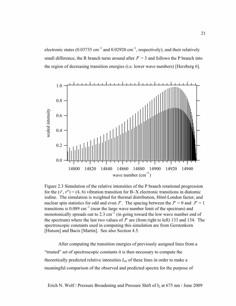
Erich N. Wolf / Pressure Broadening and Pressure Shift of I2 at 675 nm / June 2009
electronic states (0.03735 cm−1 and 0.02920 cm−1, respectively), and their relatively
small difference, the R branch turns around after J″ = 3 and follows the P branch into
the region of decreasing transition energies (i.e. lower wave numbers) [Herzberg 6].
1.0
0.8
0.6
0.4
0.2
0.0
scal
ed in
tens
ity
1494014920149001488014860148401482014800wave number (cm−1)
Figure 2.3 Simulation of the relative intensities of the P branch rotational progression for the (n′, n″) = (4, 6) vibration transition for B−X electronic transitions in diatomic iodine. The simulation is weighted for thermal distribution, Hönl-London factor, and nuclear spin statistics for odd and even J″. The spacing between the J″ = 0 and J″ = 1 transitions is 0.089 cm−1 (near the large wave number limit of the spectrum) and monotonically spreads out to 2.3 cm−1 (in going toward the low wave number end of the spectrum) where the last two values of J″ are (from right to left) 133 and 134. The spectroscopic constants used in computing this simulation are from Gerstenkorn [Hutson] and Bacis [Martin]. See also Section 4.5.
After computing the transition energies of previously assigned lines from a
“trusted” set of spectroscopic constants it is then necessary to compute the
theoretically predicted relative intensities Irel of these lines in order to make a
meaningful comparison of the observed and predicted spectra for the purpose of
22
Erich N. Wolf / Pressure Broadening and Pressure Shift of I2 at 675 nm / June 2009
assigning quantum numbers to the observed spectra. Six multiplicative factors are
generally considered to be sufficient in accounting for most of the relative intensities
of lines in a simulated spectrum of transitions between the B and X electronic states of
diatomic iodine. These factors are the Boltzmann weighting of the ground-state levels
for both vibration and rotation, the square of the electronic transition moment, the
Franck-Condon factor, the Hönl-London factor, and nuclear spin statistics [Herzberg
7].
The relative intensity Irel of a given electronic transition due to these six
multiplicative factors (taken in the same order as mentioned in the previous sentence
above) can be expressed as:
IrelHn£, J£, n≥, J≥L = N Hn≥L N HJ≥L SelHn£, n≥L
μ FCFHn£, n≥L Srot HJ£, J≥L2 J≥ + 1
Ins (2.1)
where (n″, J″) refer to the lower (or initial) state and (n′, J′) to the upper (or excited)
state. Each of the factors in equation 2.1 will be defined and described further in the
sub-sections below.
The electronic transition moment (Sel), Franck-Condon factor (FCF), and
Hönl-London factor (Srot) usually result from a quantum mechanical derivation in the
context of the Born-Oppenheimer approximation in which the solutions to the time-
independent Schrödinger equation for a molecular system are separated into electronic,
vibration, and rotation wavefunctions, respectively. The nuclear spin statistics (Ins) are
a “purely” quantum mechanical effect, which does not depend on spatial coordinates,
and does not have a classical mechanics counter-part.
For the purpose of assigning quantum numbers to the observed spectra, a
possible electronic degeneracy factor and some other physical constants can be
neglected when simulating the relative intensities of transitions between the B and X
23
Erich N. Wolf / Pressure Broadening and Pressure Shift of I2 at 675 nm / June 2009
electronic states diatomic iodine. Similarly, for the present purpose, changes in the
electronic transition moment (as a function of rotation or vibration quantum numbers)
can often be neglected, as was done in this project [Tellinghuisen].
2.4.1 Boltzmann Weighting Factors
In equation 2.1, the first two terms are the Boltzmann weighting factors Nn(n″)
and NJ(J″) for vibration and rotation, respectively. These terms account for the
fraction of molecules in a given vibration and rotation quantum state in the X
electronic state (lower energy level) at thermal equilibrium. (The probability of
finding diatomic iodine in the B electronic state is being neglected, which is
appropriate for the experimental conditions used in this project.)
The thermal distribution of quantum states Nn(n″) dependent on the vibration
quantum number n″ is then given by [Herzberg 3]:
NnHn≥L ª
N Hn≥LN
= QHnL-1 exp -EHn≥L h c
kB T (2.2)
In equation 2.2 (without loss of generality as compared to the derivations by Herzberg
[Herzberg 3]), N (n″) is the number density (i.e. number per unit volume) for the
vibration level n″ and N is the total number density; the vibration energy of the n″
level is given by E(n″) (generally in wave number units of cm−1); h is the Planck
constant, c is the speed of light (generally in cm/sec), kB is the Boltzmann constant,
and T is the absolute temperature.
24
Erich N. Wolf / Pressure Broadening and Pressure Shift of I2 at 675 nm / June 2009
The partition function (state sum) Q(v) is given by:
QHnL = ‚n≥=0
maxexp -
EHn≥L h ckB T
(2.3)
In equation 2.3, “max” refers to the highest vibration level quantum number consistent
with a bound state of the diatomic molecule (i.e. a finite internuclear separation in
Figure 2.1), and E(0) is often referred to as the zero point energy.
Determining the thermal distribution of rotational states NJ(J″) is similar to the
above case for the vibration states except that an additional factor of (2J + 1) is
included to account for degeneracy that exists in the absence of external electric or
magnetic fields. It is common practice to consider the case of a rigid rotor for which
the energy as a function of rotation quantum number is E(J) = BJ(J + 1) with B =
rotation constant (in units of cm−1). It can then be readily shown that the thermal
distribution of rotational states NJ(J″) are is well approximated by:
NJHJ≥L ª
N HJ≥LN
=B h c H2 J≥ + 1L
kB Texp -
B J≥HJ≥ + 1L h ckB T
(2.4)
2.4.2 Electronic Transition Moment
The electronic transition moment is the interaction term between the molecular
charge distribution and an electromagnetic field. Inasmuch as the electronic wave-
functions are parameterized by the internuclear separation, R, the electronic transition
moment is also a function of this variable. In “bra-ket” notation the matrix elements
for the square of the electronic transition moment is often written as Sel(n′,n″) = ⟨n′|
25
Erich N. Wolf / Pressure Broadening and Pressure Shift of I2 at 675 nm / June 2009
me(R) |n″⟩2 = | me(R) |2. For diatomic iodine the variation of this quantity as a function
of R and excitation wavelength has been partially mapped out by various researchers
for transitions between the B and X electronic states of diatomic iodine
[Tellinghuisen]. However, a meaningful functional description of the electronic
transition moment of diatomic iodine based on vibration and rotation quantum
numbers does not yet exist.
Since the electronic transition moment is typically a relatively slowly varying
quantity, and is also rather difficult to measure with any great precision or accuracy, it
is common to use an average value. While this approach is not rigorously accurate, it
is expected to suffice for the purpose of comparing a simulated spectrum to an
observed spectrum, at least when the main purpose of such a comparison is to deduce
the quantum number assignments of the states involved in the observed lines. The
agreement in comparing the relative intensities between a simulated spectrum and an
observed spectrum is expected to be reasonably accurate for transitions that span only
a few adjacent vibration levels in each of the electronic states. However, this
agreement is likely to falter a bit when using a single approximate value of the
transition moment for all rotational levels in these vibration manifolds. The relatively
congested and overlapping nature of the diatomic iodine spectrum means that a single
2 cm−1 slice of the B−X spectrum of diatomic iodine can have transitions that differ in
their rotational quantum number J″ by more than 100.
2.4.3 Franck-Condon Factor
The Franck-Condon factor is often referred to as the square of the overlap
integral of the vibration wave-functions between the two levels involved in a given
electronic transition. In modern notation this can be written as FCF(n′,n″) = ⟨n′|n″⟩2.
Since the vibration wave functions (a.k.a. eigenfunctions) are on two different
26
Erich N. Wolf / Pressure Broadening and Pressure Shift of I2 at 675 nm / June 2009
electronic surfaces they are not necessarily orthogonal to each other and so in general
this integral is not zero. In consideration of the numerous excellent expositions on the
Franck-Condon principle [Condon] it hardly seems necessary to elaborate in any great
detail on its foundations and physical interpretations. It should be noted, however,
that insofar as a given vibration wave-function will change slightly in its spatial extent
as a function of rotation level due to centrifugal distortion the Franck-Condon factor is
also a function of the rotation quantum number J. To a first approximation, though, it
is not uncommon to ignore the J dependence of the Franck-Condon factor, instead
making the approximation that the values of this factor for the non-rotating molecule
(J = 0) do not differ significantly across all values of J.
It is also worth noting that readily available algorithms that make use of
spectroscopic constants allow for computation of various spectroscopic parameters,
including the Franck-Condon factors. One such set of programs freely provided by
Professor Robert J. LeRoy accomplishes this task of computing Franck-Condon
factors by first numerically computing the potential energy surface using the semi-
classical Rydberg-Kline-Rees inversion procedure in a program named “RKR1”
[LeRoy 1]. This representation of the potential surface of a given diatomic molecule
is then readily used in a second program (referred to as “Level 7.4”) [LeRoy 2] to
numerically solve based on the Cooley-Cashion-Zare computer algorithm the radial
portion of the time-independent Schrödinger equation from which the eigenvalues E(n,
J), and the eigenfunctions |n, J⟩ are obtained. These eigenfunctions are then used to
numerically compute the Franck-Condon factors.
Using Professor LeRoy’s computer programs (and the commercially available
personal computer program SimgaPlot) it was possible to produce a slightly improved
graphical representation of the Frank-Condon factors of diatomic iodine. A previous
version [Martin] of the plot in Figure 2.4 did not include the contours indicating the
energy difference between the vibration band origins for states involved in a particular
transition. The Franck-Condon factor for a particular vibronic transition is
proportional to the area of the circle. The lack of visible circles in the lower right
27
Erich N. Wolf / Pressure Broadening and Pressure Shift of I2 at 675 nm / June 2009
quadrant of this plot would appear to be due to the Franck-Condon overlap integrals
being much smaller in magnitude than those that have a visible diameter at this scale.
Figure 2.4 Franck-Condon factors for B−X transitions in diatomic iodine (I2) as a function of vibration quantum number calculated with the use of LeRoy’s “Level 7.4” program [LeRoy 2]. The Franck-Condon factor is proportional to the area of the corresponding circle at the coordinates (n″,n′). The rotational quantum number J was set equal to zero in the calculations. The X electronic state spectroscopic constants are from Bacis [Martin]. The B electronic state spectroscopic constants that were included with LeRoy’s Level 7.4 program are from Gerstenkorn, but it is uncertain (per Professor LeRoy in a private correspondence) if this set has been published elsewhere.
28
Erich N. Wolf / Pressure Broadening and Pressure Shift of I2 at 675 nm / June 2009
2.4.4 Hönl-London Factor
The Hönl-London factor, S(J′, J″), accounts for the spatial orientation of the
transition moment of a rotating molecule with respect to a specific polarization
direction of an electromagnetic field involved in inducing transitions between the
lower and upper electronic states. This must be done for each of the (2J″ + 1)
magnetic sub-levels mJ″ of a given rotation state. The Hönl-London factor is
determined by adding together the (2J″ + 1) contributions from the individual
magnetic sub-levels for a given rotation state. In order to not over count the
contribution of this summation on the magnetic sub-levels it is necessary to divide by
the degeneracy factor (2J″ + 1), which is why the term containing the Hönl-London
factor in equation 2.1 is written as S(J′, J″) ÷ (2J″ + 1). Dividing by the degeneracy
factor of (2J″ + 1) will simply cancel the degeneracy factor appearing in the rotation
Boltzmann weighting factor above in equation 2.4.
When computing relative intensities Irel of diatomic iodine for the purpose of
assigning quantum numbers to a small slice of the spectrum (approximately 2 cm−1) it
will prove to be sufficient to use the formulas that were tabulated by Herzberg
[Herzberg 8] for the case that DL = 0; for the R branch SR(J′, J″) = (J″ + 1) and for the
P branch SP(J′, J″) = J″. More detailed considerations for deriving Hönl-London
factors can be pursued in the monograph written by Jon T. Hougen [Hougen].
2.4.5 Nuclear Spin Statistics
In order to satisfy the Pauli principle (interchange of indistinguishable particles
in the theory of quantum mechanics), homonuclear diatomic molecules in which the
29
Erich N. Wolf / Pressure Broadening and Pressure Shift of I2 at 675 nm / June 2009
two nuclei have the same isotope number will exhibit an intensity alternation between
odd and even rotation levels [Herzberg 8; Landau; Atkins]. Furthermore, for S to S
electronic transitions (in which L = 0) the intensity alternation between “strong” and
“weak” transitions will be in the ratio of (I + 1)/I where I is the quantum number of the
atomic nuclear spin. Both the B and X electronic states of diatomic iodine have L = 0,
and for the 127 isotope of iodine the nuclear spin quantum number of the nucleus is I
= 5/2, so that the intensity alternation for odd and even J″ is in the ratio of 7/5. In
calculating relative intensities of diatomic iodine the “strong” transitions occur for the
odd values of J″ (i.e., the lower level has J = 1, 3, 5…) and it is reasonable then to set
Inss = 7. The “weak” transitions occur for even values of J″ (i.e., the lower level has J
= 0, 2, 4…) for which we then use Inss = 5 [Strait].
Accounting for this intensity alternation is achieved through consideration of
the nuclear spin statistics and selection rules in conjunction with an analysis of the
nuclear hyperfine interactions (between the nuclei and electrons) in diatomic iodine.
In addition to splitting a single ro-vibronic transition into a multiplet of closely spaced
transitions that have slightly different line-centers, the nuclear spin is fundamental in
determining the relative intensity of odd and even lines. An analysis of the quantum
statistics and selection rules for B−X transitions in diatomic iodine, where both iodine
nuclei have spin I = 5/2, gives the number of possible total nuclear spin spatial
orientations (i.e. sum over degeneracy) as 21 for odd J″ and 15 for even J″ [Kroll].
2.5 Nuclear Hyperfine Structure
By the late 19th century the resolution of (electromagnetic) spectrometers had
increased to the point of revealing even finer details of the line-shape. Some of the
earliest observations of what came to be known as hyperfine structure of metallic
vapors appears to have been made by Michelson and Morley in the 1880s in their
30
Erich N. Wolf / Pressure Broadening and Pressure Shift of I2 at 675 nm / June 2009
studies of the line shape for light emitted by metallic vapors in an electric discharge
[Michelson]. A (modern) quantum theory of atomic nuclear hyperfine interactions
due to the nuclear electric quadrupole moment was first proposed by Casimir in 1936
[Casimir]. In 1940, building on Casimir’s model, Kellogg [Rabi] used molecular
beam resonance spectroscopy on the diatomic molecules HD and D2 to determine the
nuclear electric quadrupole moment of the deuterium atom. In 1945, Feld and Lamb
[Feld] provided a theoretical model for the nuclear electric quadrupole interaction of a
herteronuclear diatomic molecule in a magnetic field as a function of rotation quantum
number J. It was pointed out by Feld and Lamb that in the high-J limit (i.e. large
values of J) the interaction matrix has a diagonal asymptotic limit. A couple of years
later, Foley [Foley 1] built on the results of Feld and Lamb to provide matrix elements
for the nuclear electric quadrupole interactions in homonuclear diatomic molecules.
The nuclear hyperfine interaction in an atom or molecule is a small
perturbation caused by higher-order electromagnetic interactions among the nuclei and
electrons. The nuclear hyperfine structure is the manifestation of these interactions on
the stationary-state energy spectrum. The total electromagnetic interaction among all
electrons (m) and nuclei (n) in a system can be expressed [Cook], respectively, as
integrated charge-charge (r) and current-current (j) terms in the Hamiltonian:
HE =‡n‡
m
rnHrnL rmHrmL†rm - rn§
dvm dvn (2.5)
HM = -1c2 ‡
n‡
m
jnHrnL jmHrmL†rm - rn§
dvm dvn (2.6)
In equations 2.5 and 2.6, the charge-charge and current-current terms are functions of
position (r = (x, y, z)) and the integrals are over all space (dv = dx × dy × dz). The
speed of light c appears in the pre-factor of equation 2.6. The signs of HE and HM are
31
Erich N. Wolf / Pressure Broadening and Pressure Shift of I2 at 675 nm / June 2009
opposite, because like charges repel each other and parallel currents attract each other.
The denominator in equations 2.5 and 2.6 can be expressed as a multi-pole expansion
using spherical harmonic functions Yi(j):
†rm - rn§ = ‚k=0
¶
K 4 p2 k + 1
O rnk
rmk+1 ‚
k=0
¶
H-1Lq YqHkLHqm, fmL Y-q
HkLHqn, fnL
(2.7)
In equation 2.7 terms other than the Coulomb interaction (k = 0) are considered to be
part of the nuclear hyperfine interactions (i.e. k > 0).
A quantum mechanical derivation [Ramsey] proceeds by applying the
expansion of equation 2.7 to the Hamiltonians in equation 2.5 and 2.6. Each k-term in
HE and HM is then re-expressed as the scalar product of two irreducible tensors of rank
k with one tensor containing only electron coordinates and the other only the nuclear
coordinates. The Wigner-Eckart theorem is then used to derive the quantum
mechanical matrix elements of the nuclear hyperfine interactions for each value of k.
These matrix elements are by necessity given in a coupled representation so that it is
necessary to diagonalize the appropriate matrix (for a given k-term) on each pass
through a nonlinear regression analysis of the chromophore line-shape. The non-
vanishing off-diagonal matrix elements in the coupled representation exist because of
the selection rules that “prevent transitions between dissimilar nuclear-spin states”
[Schawlow].
From parity considerations it is possible to deduce that all odd-k terms for the
electric interaction and all even-k terms for the magnetic interaction vanish. The
leading term of the expansion (equation 2.7) for magnetic interactions is a dipole at k
= 1. This term typically arises from the magnetic dipole moment of one nucleus
interacting with the magnetic dipole created by the rotating molecule (spin-rotation
interaction). The leading term of the expansion (equation 2.7) for electric interactions
32
Erich N. Wolf / Pressure Broadening and Pressure Shift of I2 at 675 nm / June 2009
is a quadrupole at k = 2. This electric nuclear terms account for the “static” (i.e. the
illusion of a time-independent “stationary-state” consistent with a time-averaged
configuration) structure of the diatomic molecule.
2.6 Nuclear Hyperfine Structure of Diatomic Iodine
The nuclear hyperfine structure of diatomic iodine can be modeled in several
different ways, the choice of which depends on the value of J″ and the nature of the
experiment in terms of resolution and the signal-to-noise ratio (often abbreviated as
“S/N” and generally recognized as a useful indication of the detection sensitivity).
Increasingly more accurate models of the nuclear hyperfine interaction are
obtained from considering higher-order effects. The necessary higher-order
corrections (for all values of J″) come from accounting for the next k-term in
equations 2.7 commensurate with the resolution and sensitivity the spectrometer being
used to acquire such data. In 1971, Hanes, et al. [Bunker] transferred (and
transformed) Foley’s 1947 results [Foley 1] into a more modern notation. Subsequent
studies of the nuclear hyperfine structure have made use of the matrix elements given
by Hanes and even found a simpler (but equivalent) expression for Hanes, et al.
equation A4 [Borde 1; Borde 2]; that is, considerable amount of effort has gone into
verifying the quantum mechanical derivation of nuclear hyperfine interactions to this
level of description (k = 1 and 2).
An additional correction for small-J (J″ d 20) values must also be taken into
account for the perturbations due to the nearby rotation levels separated by two quanta
in each of the ro-vibronic levels [Bunker]. The contribution to the observed intensity
for transitions that result from perturbations due to these nearby rotation levels can be
expected to grow as J decreases, but exactly what the relative intensity, as compared
to the perturbations due to the same value of J as the ro-vibronic level involved in the
33
Erich N. Wolf / Pressure Broadening and Pressure Shift of I2 at 675 nm / June 2009
transition, is a more difficult problem to solve. As a result, we did not attempt to
account for the effects of these nearby rotation levels in the models used in the line-
shape analyses in this project.
In many experiments the primary goal is to “directly” measure the energy of
the nuclear hyperfine components without regard for recording an accurate line-shape;
the best relative precision frequency measurements for B−X transitions of diatomic
iodine is approaching the sub-kHz level of resolution. The increasing resolving power
and sensitivity of spectrometers has provided the opportunity to investigate the nuclear
hyperfine structure of diatomic iodine to higher-order corrections. In 1955, Schwartz
[Johnson] began the exploration of higher-order (k > 2) atomic nuclear hyperfine
interactions, beyond the electric quadrupole and magnetic dipole terms. In 1978,
Broyer, et al. [Lehmann] gave a comprehensive derivation of nuclear hyperfine
interactions in homonuclear diatomic molecules, including higher-order terms (k = 1,
2, 3, and 4), and applied these results to diatomic iodine. In 2000, Kato, et al. [Kato]
published a nuclear hyperfine-resolved atlas of diatomic iodine for the wave-number
region 15,000 – 19,000 cm−1. In 2002, Bodermann, et al. provided interpolation
formulae (accurate to about 50 kHz) for calculating the nuclear hyperfine splitting in
the region 12,195 – 19,455 cm−1 [Knöckel]. The usefulness of wavelength standards
in physics can not be easily over emphasized; Kato is simply taking the next leap in
resolution with regard to compiling a “diatomic iodine atlas” (i.e. an atlas for diatomic
iodine) [Luc 1; Luc 2; Salami].
In many instances a high-J (J″ t 20) diatomic iodine line is the subject of
investigation, which is often modeled using a “nuclear interaction” matrix in the
diagonal asymptotic limit [Kroll; Schawlow]. This situation is particularly favorable
for a line-shape analysis [Hardwick 1] since it collapses the 21 (odd J″) or 15 (even J″)
nuclear hyperfine transitions into a six groups of transitions related to each other (in
energy) by a single undetermined parameter, the difference in the nuclear electric
quadrupole coupling constant DeQq between the X and B electronic states of diatomic
34
Erich N. Wolf / Pressure Broadening and Pressure Shift of I2 at 675 nm / June 2009
iodine. The majority of the results presented in this dissertation (and certainly the
more reliable results with regard to precision and accuracy) made use of this model
based on the high-J asymptotic limit in the line-shape analyses. (See also Section 5.4.)
2.7 Frequency and Time in Spectroscopy
Modern spectroscopic methods are often broadly divided between two
categories. In one category are the time-resolved methods such as fluorescent decay
and optical photon-echo. These experiments explore dynamical properties of an
ensemble of chromophores in a non-equilibrium state prepared by (somewhat
powerful) pulses of light (a.k.a. radiation) that are comparable to or considerably
shorter in duration (Dt) than the state-changing rate of the events being observed (i.e.
measured). Decay of the (macroscopic) non-equilibrium state (usually back to thermal
equilibrium) is monitored by changes in the fluorescence emission as a function of
time.
The other category of experimental methods, which includes linear absorption
Erich N. Wolf / Pressure Broadening and Pressure Shift of I2 at 675 nm / June 2009
Third, especially in a molecule, there are state-changes that involve emission
of photons at energies that are different from (and typically smaller than) those of the
incident radiation field. And fourth, there is a spontaneous emission process, which
radiates in random directions away from the (typically well collimated) incident light
beam. In what manner (if at all) do these last two cases appear in an observed line
shape? Is the third case much like the first in which the stimulated emission is
parallel to the stimulating radiation field? In the fourth case, by what mechanism
would the total loss of a photon from the well collimated radiation field affect the
observed line shape? The tacit assumption adopted throughout this project is that all
such processes will, at a minimum, contribute to the shape (i.e. width and line-center
shift) of the radiation field transmitted through an absorption medium [Barut 1].
The inhomogeneous contribution to the observed (frequency domain) line-
shape is the result of processes that are not the same for all of the constituents in the
absorption medium. For molecules in the gas phase at a relatively low pressure, this
contribution appears to be described quite well by Doppler broadening, for which a
quantitative model is obtained by consideration of the Maxwell-Boltzmann
distribution of velocities, which can be related to the distribution of resonant (line-
center) frequencies w0 = 2n0 in the gas sample for thermal equilibrium at a temperature
T. In the laboratory frame the radiation frequency is un-shifted, and the distribution of
molecular velocities parallel to the propagation direction of the radiation field can be
modeled by a shift in the resonant frequency such that the resonant frequency is given
by w0′ = (1 ± v/c) w0 in the reference frame of the molecules, where v is the speed of a
molecule along the propagation direction of the radiation field, c is the speed of light,
and w0′ is the frequency of the radiation field in the laboratory reference frame. The
inhomogeneous width of the line-shape is then found to have the functional form of a
Gaussian (Normal) distribution [Bernath]. It is also common (in time domain models)
for this width to be referred to as a decay time-interval T2*, which can then be
expressed as the decay rate 1/T2* [Allen 2]. Conceptually, the inhomogeneous decay
rate 1/T2* can be thought of as the rate at which the line-center frequencies in the
39
Erich N. Wolf / Pressure Broadening and Pressure Shift of I2 at 675 nm / June 2009
ensemble of transition moments (i.e. large collection of chromophores) de-phase (i.e.
precess) relative to each other during the period of “interaction-free” translational
motion between all types of collision events, including those collision events that do
not result in an appreciable, or perhaps perceptible, state-change of the radiation field.
In the case of transitions in the visible (a.k.a. optical) portion of the
electromagnetic spectrum the inhomogeneous contribution (Doppler/Gaussian) to the
line-shape is generally much larger than the homogeneous (Lorentzian) portion for
relatively low total gas pressure (up to a few tens of torr in the case of diatomic iodine).
The homogeneous width is typically observed to increase linearly as the pressure of
buffer gas is increased. At about 100 torr of buffer gas, the homogeneous width of
diatomic iodine is comparable in magnitude to the constant Doppler width. In the case
of diatomic iodine, the theoretical Doppler width (full width at half maximum
intensity) is 341 MHz at room temperature (292 K) and transition energy of 14,818
cm−1 (corresponding to a radiation wavelength of approximately 675 nm); see also
Section 5.2 for more details. (However, due to the rather large nuclear hyperfine
splitting, a high resolution spectrum of a well isolated ro-vibronic transition at a
pressure of about 0.2 torr has an (observed) Doppler-broadened width of roughly 600
MHz.)
2.9 The Two-Level System Model
The basic two-level system model offers a description of energy exchange
processes between a chromophore and radiation field. There are three distinct
processes shown in Figure 2.5. The two processes on the left-hand side of Figure 2.5
– stimulated absorption and emission of radiation and spontaneous emission (of
photons) – do not depend on collisions with a buffer gas and so do not depend on the
pressure (a.k.a. pressure-independent). The right-hand side of Figure 2.5 depicts the
collision-induced stimulated photon absorption and emission process and it does
40
Erich N. Wolf / Pressure Broadening and Pressure Shift of I2 at 675 nm / June 2009
depend on the pressure (a.k.a. pressure-dependent). As usual, the stimulated processes
are presumed to be “coherent” with the incident radiation field: it is presumed (with or
without a collision event) that the photon emitted during stimulated emission has the
same phase as the radiation field involved in the stimulation process, and that it
propagates in the same direction as this stimulating field; it is presumed that a
stimulated absorption event has a strong orientation effect on the transition moment of
the chromophore. And it is presumed that the spontaneous emission events occur in
completely random spatial directions and have no phase relationship with the
(typically well collimated) radiation field.
Figure 2.5 The two-level system model depicting three state-changing processes (from left to right): pressure-independent stimulated absorption and emission of photons (“rad. stim.”), spontaneous emission of photons (“spont. emis.”), and pressure-dependent (i.e. collision-induced) stimulated absorption and emission of photons (“coll.-rad. stim.”). On the left-hand side of this figure are the energies of the stationary-states (Ñwg and Ñwe) and the transition (and photon) energy DE. On the far right-hand side of this figure is the “ket” designation of the steady-states (|g⟩, and |e⟩), and the number densities of these two states (Ng and Ne) in the ensemble (integrated over all frequencies w). The ensemble-average photon absorption and emission rates of the three processes are given (from left to right) by rabs, rem, Asp, cabs, and cem, with the subscripts “abs” and “em” respectively indicating absorption and emission, and “sp” for spontaneous emission.
Upon turning-off the radiation field, the spontaneous emission process will
continue to operate in its usual manner. The photons emitted by spontaneous emission
might provide the photons for collision-induced stimulated emission, or (perhaps) an
entirely different (but similar) collision-induced emission process could be operating.
rad. stim. spont. emis. coll.- rad. stim.
DE = Ñw
|e⟩, Ne
Ñwg
Ñwe
Asp
|g⟩, Ng
cem cabsrabs rem
41
Erich N. Wolf / Pressure Broadening and Pressure Shift of I2 at 675 nm / June 2009
With respect to the spontaneously emitted photons, the pressure-independent
stimulated absorption and emission and the collision-induced stimulated absorption
processes could still be active, but their effects are expected to be rather negligible.
Whatever the events that lead to decay, the propagation of photons will appear to
occur in random spatial directions. The ensemble of chromophores will decay towards
a distribution of states consistent with thermal equilibrium; at optical frequencies this
equilibrium state has nearly all of the chromophores in the lower energy level
(designated as |g⟩ in Figure 2.5).
In time-resolved experiments using relatively short duration pulses of light (at
or near visible frequencies), the non-equilibrium state is presumed to be (coherently)
prepared by the pressure-independent stimulated absorption process (given by the rate
rabs on the left-hand side of Figure 2.5). The ensemble-average decay rate of the
prepared collection of chromophores in the upper energy level is often characterized
symbolically as 1/T1, which can be sub-divided into a contribution from the (pressure-
independent) spontaneous emission process and another from the (pressure-dependent)
collision-induced emission process: 1/T1 = Asp + cem. An example of an experiment
that can measure the random events that contribute to 1/T1 is fluorescent decay
[Paisner].
The two-level system model is fairly ubiquitous and is generally regarded as
being rather useful. As a complement to this point of view, an outline of a kinetic
model based on ensemble-average transition rates for steady-state linear absorption
will be presented in Section 2.11, one which might prove useful in the measurement of
transition moments. However, the two-level system model described in this section
only accounts for energy exchange between the chromophore in one particular total
stationary-state (i.e. ro-vibronic and translational) and the radiation field. Even though
a collision-induced photon absorption and emission mechanism (i.e. a cause) has been
included, this model is not able to account for energy exchange due to collisions with
a buffer gas. Furthermore, the two-level system model does not consider in a more
general manner the nature of collision-induced phase-changes of the radiation field,
42
Erich N. Wolf / Pressure Broadening and Pressure Shift of I2 at 675 nm / June 2009
which will be addressed in the next section by the addition of two more “levels” to this
model.
2.10 The Four-Level System Model
In order to account for a process that is perhaps more fundamentally related to
the wave-nature of the radiation field (i.e. phase-change, as opposed to energy
exchange in the particle-nature point of view), two levels have been added to the two-
level system model to form the basis for a four-level model. The four levels are
depicted in Figure 2.6. To simplify the model, the |g′⟩ and |e′⟩ states are here taken as
being respectively in the same “ro-vibronic” (or electronic) states as the |g⟩ and |e⟩
states, but representing different translational states. The transition from |g⟩ to |g′⟩ or
|e⟩ to |e′⟩ (or vice versa) occurs through a collision with a buffer gas, which can be
envisaged as resulting in a change in the velocity (in a vector sense) of the
chromophore.
Figure 2.6 The four-level model depicting phase-changing state-changes between |g⟩ and |g′⟩ and transitions between |e⟩ to |e′⟩ due to collisions with a buffer gas. Each pair of states ( |g⟩, |e⟩ ) and ( |g′⟩, |e′⟩ ) satisfies the two-level system model of Figure 2.5. The ensemble-average phase-changing rates (of the radiation field) are given by fg, fg′, fe, and fe′. In general, it is expected that w ≠ w′.
Ñw Asp
cemcabsrabs rem
|g⟩
|e⟩
Ñw′Asp′
cem′ 1
cabs′ rabs′ rem′
|g′⟩
|e′⟩ fe′
fe
fg
fg′
43
Erich N. Wolf / Pressure Broadening and Pressure Shift of I2 at 675 nm / June 2009
It can be envisaged that at some point in time and space during the course of a
collision (perhaps in a deterministic sense) the phase of the radiation is “suddenly”
disrupted (i.e. changed to a meaningful extent in an almost discontinuous manner).
This phase-change of the radiation field is generally modeled as involving a
significant change in the orientation of the transition moment, such that (some form of)
an interaction between the chromophore and radiation field is disrupted. The change
in velocity of the chromophore (due to a collision event) also means that its transition
energy is slightly altered (relative to the laboratory frame due to the Doppler Effect);
i.e. w ≠ w′. As Figure 2.7 indicates, by including (more explicitly) the possibility for
velocity-changes during a collision event, the four-level model, even in this limited
form, makes more transparent the possible range of pressure-dependent processes.
Figure 2.7 The four-level model depicting (some of the) possible paths for the state-changing process.
In time-resolved (non-equilibrium) experiments (using relatively short duration
pulses of light), the total decay rate due to homogeneous processes can be expressed
(i.e. modeled) as the sum of two ensemble-average rates, the photon emission rate for
fluorescent decay 1/T1 (mentioned at the end of the last section) and the rate of
collision-induced (i.e. pressure-dependent) phase-changes of the transition moment fe
for |e⟩ → |e′⟩ transitions, which can be written symbolically as 1/T2′ = 1/T1 + fe. An
example of an experiment that measures (i.e. observes) this decay time is the optical
photon echo [Dantus].
Ñw
|g⟩
|e⟩
Ñw′
|g′⟩
|e′⟩
44
Erich N. Wolf / Pressure Broadening and Pressure Shift of I2 at 675 nm / June 2009
2.11 Steady-State Kinetic Model
An important objective in building two-level and four-level system models is
to decipher the information content encoded in an observed steady-state linear
absorption line shape (i.e. spectrum). In this section we will seek to justify a kinetic
model for the two-level system and then explore its implications, especially with
regard to the underlying dynamics of the observed steady-state linear absorption line
shape. This model differs slightly from the usual “A and B Coefficient” model
[Einstein], but perhaps we should keep in mind that the model developed by Einstein
was intended for a perfectly isolated (but non-existent) black-body radiator based on
the ratio of (single temperature T thermal equilibrium) Boltzmann distributions for the
two energy levels (in the two-level system model). Perhaps it is fair (or reasonable) to
claim that the A and B Coefficient model describes a realm of steady-state state-
changing behavior from a point of view that is not quite consistent with the steady-
state state-changing condition created by directing a well-collimated external source of
relatively low-intensity, narrow bandwidth radiation to pass through an absorption
medium.
A meaningful goal of any two-level system model (e.g. Figures 2.5) is to
derive (or re-derive) the Beer-Lambert law from the microscopic point of view. The
Beer-Lambert law is an empirical observation about steady-state linear absorption of
radiation by a large ensemble of chromophores, often expressed in the differential
form as „I(z)/„z = −kI(z), which leads to the integrated form:
I HHw0 - w0≥L, zL = I HHw0 - w0
≥L, 0L expH-k zL
ª I HzL = I H0L expH-k zL (2.8)
45
Erich N. Wolf / Pressure Broadening and Pressure Shift of I2 at 675 nm / June 2009
In equation 2.8, I(z) ª I((w0 − w0″), z) is the line-integrated radiation field intensity (i.e.
the total intensity of the radiation field across all frequencies w) after passing though
an absorption medium of length z; the radiation field initially incident on the
absorption medium (at z = 0) has a line-integrated intensity I(0) ª I((w0 − w0″), 0); and
k is the absorption coefficient (a characteristic constant of the absorption medium at a
given pressure and temperature). The radiation field line-center frequency w0″ is often
the same as the observation frequency (as was the case in this project). The intensity
of the radiation field is thus properly described by the difference in the chromophore
line-center frequency w0 and the observation frequency w0″.
Intensity has units of energy per unit area per unit time. One of the hallmarks
of linear absorption (worthy of considerable emphasis) is that the ratio I((w0 − w0″), z)
÷ I((w0 − w0″), 0) is constant for a broad range of initial intensities I((w0 − w0″), 0).
Also, without loss of generality, the following descriptions will use the simplifying
assumption that the incident radiation field intensity I((w0 − w0″), 0) is equal to a
constant value across a broad range of radiation field line-center frequencies w0″ (i.e.
the ideal case of the radiation field being independent of the absorption medium); see
also Section 5.3.
Whatever the experimental conditions may be, and whatever state-changing
processes might be envisaged as operating, a steady-state condition is achieved in the
two-level system model when the differential change in the population densities of the
ground and excited states with respect to time has vanished:
„ Ne„ t
= -„ Ng
„ t= 0
(2.9)
In equation 2.9, the total number densities for a particular radiation field line-center
frequency w0″ (a.k.a. line-integrated number density) for the two-level system model
are given by Ng and Ne.
46
Erich N. Wolf / Pressure Broadening and Pressure Shift of I2 at 675 nm / June 2009
From the point of view of the chromophore, application of equation 2.9 (for the
two-level system model of described in Section 2.9 and Figure 2.5), where the sum of
ensemble-average stimulated photon absorption and emission rates are given
respectively by kabs = rabs + cabs and kem = rem + cem, gives:
-Asp Ne - kem Ne + kabs Ng = 0 (2.10)
From the point of view of the externally applied (and typically well collimated)
radiation field, the observed change in the total (line-integrated) intensity as a function
of path length can be expressed as:
„ I HzL„ z
= H- Asp Ne + kem Ne - kabs NgL Ñw0 (2.11)
The observed line-center frequency w0 is being used (on the right-hand side of
equation 2.11) on the pretense that the energy of a photon (E = wÑ) does not change to
an appreciable extent across a relatively narrow frequency-interval of the Doppler and
collision broadened radiation field line shape at optical frequencies.
Substitution of equation 2.10 into equation 2.11 gives:
„ I HzL„ z
= -2 Ñw0 Asp Ne = 2 Ñw0 Hkem Ne - kabs NgL (2.12)
The next step is to reconstruct equation 2.12 from the point of view of the
microscopic processes that give rise to I(z) ª I((w0 − w0″), z) and Ne ª Ne(z) ª Ne((w0
− w0″), z). This reconstruction will be achieved through the convolution of
independent processes (i.e. homogeneous and inhomogeneous line broadening
mechanism) [Demtröder, Butkov]. Two successive convolutions will be performed,
47
Erich N. Wolf / Pressure Broadening and Pressure Shift of I2 at 675 nm / June 2009
so it is useful to note that the order in which convolutions are performed can be
arbitrarily chosen. In the language of mathematics, the convolution procedure obeys
the commutative, associative, and distributive properties. The first two properties are
relevant to what follows in this section, namely that f * g = g * f and f * (g * h) = (f * g)
* h [Kauppenin].
The intensity of the radiation field per unit bandwidth interval Iw(((w0 − w0″) −
w), z) can be described by the following distribution function:
IwHHHw0 - w0≥L - wL, zL
= I HHw0 - w0≥L, zL ²R gRHHw0 - w0
≥L - wL
ª I HzL ²R gRHHw0 - w0≥L - wL (2.13)
Equation 2.13 describes the radiation field intensity per unit bandwidth interval
relative to the difference of the observed line-center frequency w0 and the radiation
field line-center frequency w0″ as a fraction of the total radiation field intensity I((z) ª
I((w0 − w0″), z) (across all frequencies w) at a particular position z in the absorption
medium. The distribution function gR((w0 − w0″) − w) has a normalization factor
given by ²R:
²R ‡
0
¶gRHHw0 - w0
≥L - wL „ w = 1 (2.14)
48
Erich N. Wolf / Pressure Broadening and Pressure Shift of I2 at 675 nm / June 2009
Standard (or classical) treatments of electromagnetic wave propagation
indicate that the cycle-averaged radiation field intensity I((z) ª I((w0 − w0″), z) is
related to the electric field strength E(z) ª E((w0 − w0″), z) by:
I HzL =
12
c h e0 †EHzL§2 (2.15)
In equation 2.15, c is the speed of light in a vacuum, h is the index of refraction, and e0
is the vacuum permittivity.
The anticipated steady-state probability |ce(w0 − w)|2 of finding a given
chromophore in the excited-state contains a contribution from the square of the
radiation field strength |E((w0 − w0″), z)|2 ª |E(z)|2 (e.g. see equation 7.36). Equation
2.15 then says that this contribution is directly proportional to the radiation field
intensity I(z) ª I((w0 − w0″), z). However, a more realistic description of a radiation
field acknowledges the nonexistence of such fields being perfectly monochromatic,
which is achieved with a distribution function of finite width and having units of
intensity per unit bandwidth interval (e.g. equation 2.13).
Likewise, the distribution for the excited-state probability |ce(w0 − w)|2 is
converted to a probability density characterizing the excited-state probability per unit
bandwidth interval. The portion pertaining to the radiation field has been factored out
of |ce(w0 − w)|2, so that the remaining core portion of this distribution ( |ce′(w0 − w)|2 )
can be expressed as:
†ce
£Hw0 - wL§2 =2 m2
c h e0 Ñ2 ²e geHw0 - wL
(2.16)
49
Erich N. Wolf / Pressure Broadening and Pressure Shift of I2 at 675 nm / June 2009
In equation 2.16, the distribution function ge(w0 − w) is normalized by ²e:
²e ‡
0
¶geHw0 - wL „ w = 1
(2.17)
The transformation of the descriptions of the radiation field and excited-state
probability into probability density functions (of finite widths that describe the
associated quantities per unit bandwidth interval) then leads to the steady-state
probability |ce″((w0 − w0″) − w)|2 of finding a given chromophore in the excited-state
per unit bandwidth interval:
†ce≥HHw0 - w0
≥L - wL§2
= ‡0
¶†ce
£Hw0£ - wL§2 I HHHw0 - w0
≥L - w0£L, zL „ w0
£
=2 m2 I HzLc h e0Ñ
2 ‡0
¶²e geHw0
£ - wL
μ ²R gRHHw0 - w0≥L - w0
£L „ w0£
ª2 m2 I HzLc h e0Ñ
2 ²H gHHHw0 - w0≥L - wL
(2.18)
In equation 2.18, m is the electronic dipole transition moment. The subscript “H” on
gH((w0 − w0″) − w) is in anticipation of this distribution function being commensurate
with the homogeneous contribution to the observed line shape.
50
Erich N. Wolf / Pressure Broadening and Pressure Shift of I2 at 675 nm / June 2009
The normalization factors ²R and ²e in equations 2.14 and 2.17 require
considerable care when proceeding through this analysis. The normalization factor
obtained by the convolution of distribution functions is in general a function of the
normalization factors of the convolved components. In equation 2.18, the explicit
expression of this point can be given as ²H = ²H (²R, ²e). For the case that the gR and
ge are both described by Lorentzian distributions, it can be readily shown that the
normalization factor is given by ²H = ²R + ²e , in which ²R and ²e are simply related
to the full width at half-maximum height of gR(w0 − w0″) − w) and ge(w0 − w),
respectively [Loudon 1; Bernath; see also equations 5.3 and 5.4].
The second convolution is between the result of the convolution in equation
2.18 and the inhomogeneous contribution to the observed line shape, in this case taken
to be well described by the Doppler profile. In a typical gas cell the total number
density (of chromophore) per unit bandwidth interval N (w0 − w) is distributed in the
frequency domain according to the normalized Doppler profile ²D gD(w0 − w)
[Bernath]:
N Hw0 - wL = N ²D gDHw0 - wL
=2 p N
w0
m c2
2 p kB T
1ê2exp -
m c2
2 kB Tw0 - w
w0
2
(2.19)
In equation 2.19, N is the total number density of the chromophore (and N = Ng + Ne),
m is the mass of the chromophore, c is the speed of light in a vacuum, T is the
temperature, and kB is the Boltzmann constant; gD is given by the exponential factor
[Bernath].
51
Erich N. Wolf / Pressure Broadening and Pressure Shift of I2 at 675 nm / June 2009
The excited-state number density per unit bandwidth interval Ne((w0 − w0″) −
w) at a particular radiation field line-center frequency w0″ is then given by the
convolution of equations 2.18 and 2.19:
NeHHw0 - w0≥L - wL
= ‡0
¶†ce
≥HHw0 - w0≥L - w0
£L§2 N Hw0£ - wL „ w0
£
=2 N m2 I HzL
c h e0 Ñ2 ‡
0
¶²H gHHHw0 - w0
≥L - w0£L
μ ²D gDHw0£ - wL „ w0
£
ª2 N m2 I HzL
c h e0 Ñ2 ²V gVHHw0 - w0
≥L - wL
(2.20)
In equation 2.20, the subscript “V” on gV((w0 − w0″) − w) is in anticipation of this
distribution function being well modeled as a Voigt profile. And it is worth noting
that the normalization factor for the Voigt profile is dependent on the underlying
distribution functions: ²V = ²V(²H, ²D). In this project, for which the radiation field
line shape and temperature were held constant, changes in buffer gas pressure affect
the width of ge((w0 − w) and thus ²e., which in turn affects the normalization factor ²V
of the Voigt profile; see also Section 5.3.
52
Erich N. Wolf / Pressure Broadening and Pressure Shift of I2 at 675 nm / June 2009
The more general form of equation 2.12 for per-bandwidth-interval distributions (e.g.
probability density functions) is given by:
„ IwHHHw0 - w0≥L - wL, zL
„ z= -2 Ñw0 Asp NeHHw0 - w0
≥L - wL
(2.21)
Using equations 2.13 and 2.14, integration of the left-hand side of equation
2.21 across all frequencies w gives:
‡0
¶ „ IwHHHw0 - w0≥L - wL, zL
„ z„ w
=„ I HHw0 - w0
≥L, zL„ z ‡
0
¶²R gRHHw0 - w0
≥L - wL „ w
=„ I HHw0 - w0
≥L, zL„ z
ª„ I HzL
„ z (2.22)
53
Erich N. Wolf / Pressure Broadening and Pressure Shift of I2 at 675 nm / June 2009
Using equation, 2.20, integration of the right-hand side of equation 2.21 across
all frequencies w gives:
-2 Ñw0 Asp ‡0
¶NeHHw0 - w0
≥L - wL „ w
= -2 Ñw0 Asp Ne
= -4 w0 Asp N m2 ²V I HzL
c h e0 ч
0
¶gVHHw0 - w0
≥L - wL „ w
ª -K I HzL‡0
¶gVHHw0 - w0
≥L - wL „ w
(2.23)
Substitution of equations 2.22 and 2.23 into equation 2.21, followed by
rearrangement and integration yields the Beer-Lambert law:
I HzL = I H0L expK-K K‡
0
¶gVHHw0 - w0
≥L - wL „ wO zO (2.24)
Equation 2.24 indicates that for each value of the radiation field line-center frequency
w0″ the distribution of transmitted light follows a Voigt-like profile gV ((w0 − w0″) − w)
defined in equation 2.20. As the radiation field line-center frequency w0″ is scanned
across the absorption profile, the integration of this underlying Voigt-like distribution
across all frequencies w is traced out in the recorded spectrum; recall that I((z) ª I((w0
− w0″), z) and I((0) ª I((w0 − w0″), 0).
Not shown explicitly in the preceding developments (in equations 2.18 through
2.24) is a convolution of the detector response with the transmitted radiation field. To
54
Erich N. Wolf / Pressure Broadening and Pressure Shift of I2 at 675 nm / June 2009
the extent that a detector has a flat response across a relatively broad spectral region
that includes and is much broader than the spectral region of interest (i.e. the transition
line shape encoded in the transmitted radiation field), the detector response gd(w − wd)
can be factored out of the corresponding convolution integral in the (approximate)
form g × (Dwd)−1, where Dwd is the bandwidth of the detector, g is a dimensionless
instrument function, and wd is the center frequency of the detector. Integration of the
left-hand side of equation 2.21 then gives:
‡0
¶ „ IwHHw0 - w0≥L - wL, zL
„ z„ w
= ‡0
¶K „
„ z ‡0
¶gdHw - wdL I HzL ²R gRHHw0 - w0
≥L - wL „ wO „ w
@g
Dwd
„ I HzL„ z ‡
0
Dwd„ w ‡
0
¶²R gRHHw0 - w0
≥L - wL „ w
=g
Dwd
„ I HzL„ z
HDwdL 1 = g„ I HzL
„ z (2.25)
55
Erich N. Wolf / Pressure Broadening and Pressure Shift of I2 at 675 nm / June 2009
Integration of the right-hand side of equation 2.21 treats the Voigt profile
gV((w0 − w0″) − w) as a Dirac-delta function, which filters out its value at w = w0 −
w0″ (i.e. gV(w0 − w0″):
-2 Ñw0 Asp NeHHw0 - w0≥L - wL
= -2 Ñw0 Asp ‡0
¶K‡
0
¶gdHw - wdL NeHHw0 - w0
≥L - wL „ wO „ w
@ -Kg I HzLDwd
‡0
Dwd„ w ‡
0
¶gVHHw0 - w0
≥L - wL „ w
@ -Kg I HzLDwd
HDwdL gVHw0 - w0≥L
= -K g I HzL gVHw0 - w0≥L
(2.26)
Combining equations 2.25 and 2.26 (and recalling that I(z) ª I((w0 − w0″), z))
leads to the more familiar form of the Beer-Lambert law given by equation 2.12 (as
opposed to equation 2.21):
g„ I HHw0 - w0
≥L, zL„ z
= -2 Ñw0 Asp g NeHw0 - w0≥L
= -K g I HHw0 - w0≥L, zL gVHw0 - w0
≥L (2.27)
56
Erich N. Wolf / Pressure Broadening and Pressure Shift of I2 at 675 nm / June 2009
In equation 2.27, the observation frequency is given by the radiation field line-center
frequency w0″, which corresponds to the experimental configuration used in this
project. Rearrangement and integration of equation 2.27 then leads to the often used
form of the Beer-Lambert law in high-resolution linear absorption experiments (c.f.
equation 2.8), especially for the task of performing a line shape analysis:
I HHw0 - w0≥L, zL = I H0L expH-K gVHw0 - w0
≥L zL (2.28)
See also Sections 5.2 and 5.3, especially equation 5.3, and recall that w = 2pn.
As equation 2.24 (or equation 2.28) indicates, one reason for considering the
details of deriving the Beer-Lambert law from the microscopic point of view is to
relate measurements of line shape and line-integrated radiation field intensity to the
transition moment m of the chromophore. However, such measurements are not
pertinent to the results presented in this dissertation. Another reason for deriving a
model of the Beer-Lambert law based on microscopic processes of equations 2.10 and
2.11 is to gain some confidence in their validity.
The main reason for pursuing the above developments in this section has to do
with a central question in spectroscopy: what is the information content encoded in an
observed line shape? Equation 2.12 (or equation 2.21) indicates that the observed line
shape will be influenced by both the absorption and emission processes [Barut 1].
Furthermore, the steady-state kinetic model developed in this section is consistent with
classical equilibrium thermodynamics; such considerations lead to results (described
below) that will be important in the analysis of state-changing processes later in this
dissertation, specifically Section 6.3 and Chapter VII.
57
Erich N. Wolf / Pressure Broadening and Pressure Shift of I2 at 675 nm / June 2009
If we tacitly recognize that the kinetic model for the two-level system
presented so far accounts for an essential portion of the physics of linear absorption,
then comparison of equation 2.10 to the Boltzmann distribution gives:
NgNe
=Asp + kem
kabs= exp
Ñw0kB T
> 1
ï Asp + kem > kabs (2.29)
The temperature T appearing in equation 2.29 is a characteristic temperature of the
steady-state state-changing process, which is not the same as the usual sense of this
parameter (as used throughout this dissertation) for describing the center-of-mass
motion (a.k.a. translation) of an atomic system.
The time domain view of the inequality in equation 2.29 is depicted in Figure
2.8. This inequality indicates that the ensemble-average time-interval Dtabs between
|g⟩ → |e⟩ (photon absorption) state-changing events is longer than the time-interval
Dtem between |e⟩ → |g⟩ (photon emission) state-changing events; in Chapters VI and
VII, the notation for this inequality on the time-intervals between state-changing
events will appear as tem ∫ t abs.
Figure 2.8 Ensemble-average state-changes in the time domain depicting the inequality of equation 2.17 in which Dtabs > Dtem. The ensemble-average time-interval between |g⟩ → |e⟩ and |e⟩ → |g⟩ state changes are given respectively by Dtabs and Dtem.
|g⟩ |e⟩ |g⟩ Dtabs = 1/kabs Dtem = 1/(Asp + kem)
t
58
Erich N. Wolf / Pressure Broadening and Pressure Shift of I2 at 675 nm / June 2009
Collision cross-sections are described in more detail in Sections 6.3 and 7.5.
The concept of a collision-cross section will be utilized in the last few paragraphs of
this section. So, for pedagogical purposes, perhaps it is useful to mention that a
collision cross-section is essentially “an (effective) area representative of a collision
reaction between atomic or nuclear particles or systems, such that the number of
reactions that occur equals the product of the number of target particles or systems and
the number of incident particles or systems which would pass through this area if their
velocities were perpendicular to it [McGraw-Hill].” This concept is often expressed as
1/t0 = nsv, where t0 is the ensemble-average time-interval between collision events, n
is the number density of atomic systems, s is the collision cross-section, and v is the
ensemble-average relative speed between these atomic systems [Reif].
For a situation in which the radiation stimulated photon absorption and
emission (and spontaneous emission) are the dominant state-changing processes,
collision cross-sections for photon absorption (sabs) and emission (sem) can be
constructed from the rate of change of rem and rabs with that of the radiation field
intensity. In the abstract sense of considering a collision cross-section function of the
form rabs = sabsf(I(z)) and rem = semf (I(z)) (i.e. linearization of I(z) with respect to the
pressure-independent photon absorption and emission rates), then for ∑Asp/∑(f (I(z)) =
0 (a typical assumption that may require further consideration [Allen 3]) equation 2.29
leads to:
J ∑ rem∑ f HIHzLL
N
J ∑ rabs∑ f HIHzLLN
=semsabs rad. stim.
> 1
(2.30)
In equation 2.30, the symbol “∑” indicates a partial derivative; e.g. the denominator
means taking the partial derivative of rem with respect to f (I(z)).
59
Erich N. Wolf / Pressure Broadening and Pressure Shift of I2 at 675 nm / June 2009
Similarly, and of relevance to the pressure-dependent studies presented in this
dissertation (see also Sections 6.3 and 7.5), if the radiation field intensity is held
constant and the pressure P is changed, then ∑rabs/∑P = ∑rem/∑P = ∑Asp/∑P = 0. The use
of an ideal gas-kinetic model for the collision-induced collision cross-section (applied
to the two-level system model of Section 2.9) gives cabs and cem as being linearly
related to the pressure P, so that equation 2.29 leads to:
J∑ cem∑ P
N
J ∑ cabs∑ P
N=
semsabs coll.-rad.stim.
> 1
(2.31)
Only the change in width of the line shape is relevant when measuring
pressure-dependent (elastic) collision cross-sections (sabs and sem) and so the increase
in the ratio of I(z) to I(0) can be ignored when measuring the self-quenching collision
cross-section. In this case, the pressure P is due entirely to the number density n of
chromophores (through the ideal gas law), and so the number density n of
chromophores must be changed in order to affect a change in pressure P. And
equation 2.31 is expected to be valid for the case of holding the chromophore number
density constant and relatively small compared to the number density n of a buffer gas,
as was done for the measurement of collision cross-sections in this project.
Equation 2.31 is a statement from classical (equilibrium) thermodynamics,
which says explicitly that sem > sabs. The importance of this inequality is substantial.
And it is perhaps still an open question as to whether or not a dynamical theory like
quantum mechanics can or should be able to account for the “conclusions” obtained
from classical thermodynamics.
It should be understood that the use of the same notation for the collision
cross-sections (sabs and sem) in equations 2.30 and 2.31 is not meant to imply that
these quantities are the same for these two different processes, which is why the
60
Erich N. Wolf / Pressure Broadening and Pressure Shift of I2 at 675 nm / June 2009
subscripts “rad. stim.” and “coll.−rad. stim.” have been appended to these ratios in the
above respective equations; see also Figures 2.5 and 2.6.
An obvious question arises: what might be the connection between the model
developed in this section for linear absorption and the well respected A and B
Coefficient model? The energy density of the radiation field W(x, y, z) is related to the
intensity of the radiation field I(x, y, z) by I(x, y, z) = cW(x, y, z), where c is the speed
of light in a vacuum. The Einstein model for a steady-state black-body radiator can be
expressed as AspNe + BegI(z)Ne − BgeI(z)Ng = 0, and it is generally assumed that Bge =
Beg. Furthermore, for the black-body radiator model used by Einstein (i.e. the Plank
law for the radiation field energy density in a perfectly isolated black-body radiator, or
Planck radiation law), the single temperature T of the black-body radiator would
appear to imply that the radiation field intensity I(x, y, z) is the same at all locations (x,
y, z), which can be expressed as I(x, y, z) = constant. This condition of constant
radiation field intensity I(x, y, z) does not appear to be consistent with linear
absorption as described by equation 2.8 (i.e. „I(z)/„z = −kI(z) ∫ 0). It is beyond the
scope of this dissertation to consider modifying the underlying Planck radiation law
used in the Einstein A and B Coefficient model to account for the change in radiation
field intensity I(x, y, z) as a function of position (x, y, z), therefore, as hinted at the
beginning of this section, it has been tacitly assumed that it is possible to approach the
Einstein A and B Coefficient model in a way that is consistent with the Beer-Lambert
law for steady-state linear absorption. It is worth noting, though, that the inequality
kem ∫ kabs (suggested by equation 2.29) would appear to be related to the suggestion
that Bge ∫ Beg [Mompart].
Further comparison of the Einstein A and B Coefficient model and the Beer-
Lambert law does not appear to be appropriate or necessary at this time. However, the
question (of mechanism) has been raised as to how a black-body radiator progresses
towards a state of thermal equilibrium with a material system (e.g. a two-level system)
[Irons]. An answer to this question (in terms of the concepts of irreversibility and
dissipation of heat energy) is offered at the end of Chapter VII.
61
Erich N. Wolf / Pressure Broadening and Pressure Shift of I2 at 675 nm / June 2009
2.12 Collision Processes
Atoms and molecule are complex objects, each one being composed of a finite
number of electrons and nuclei. In the ideal but non-existent limit of a perfectly
isolated atomic (or molecular) system, time-independent quantum mechanics can be
characterized by stationary-states, which is a useful description of the properly time-
averaged internal dynamical properties of such a system. However, contained within
the idea of a perfectly isolated stationary-state is the reality that such an object would
reside in a universe where there is “a time without time”, or perhaps more accurately,
“a time without change”. A more generally approach, then, would seek to model the
interactions between atomic systems through considerations of time-dependent
dynamics.
As described in Sections 2.9 and 2.10, some portion of the interactions
between a chromophore and buffer gas particle can be characterized by collision-
induced state-changing rates. The notion of a purely elastic collision (often modeled
as instantaneous collisions between infinitely-hard (i.e. non-deformable) spheres) is
useful in a conceptual sense, but it is only an idealization that does not appear to exist
in Nature; it appears that all collisions are, to some degree or another, inelastic. It is
also common to associate the phrase “inelastic (state-changing) collisions” with
changes in the internal time-independent stationary-states of an atomic system; e.g. the
state-changing processes that involve photon absorption and emission [Steinfeld].
These stationary-states are consistent with the solutions obtained from solving the
time-independent Schrödinger equation for the case of a perfectly isolated
chromophore. However, with or without such internal state-changes, the inelastic
nature of collisions can be expected to contribute to changes in the translational
motion (i.e. trajectories) of the collision partners (e.g. chromophore and buffer gas),
and thus changes in the spatial (and perhaps temporal) orientation of the chromophore
62
Erich N. Wolf / Pressure Broadening and Pressure Shift of I2 at 675 nm / June 2009
transition moment with respect to, say, a linearly polarized radiation field (e.g. like the
ones used in this project).
The “traditional” solution of the time-dependent Schrödinger equation for the
two-level system model does not include a cause that leads to the effect of photon
absorption and emission [Bernath]. In Chapter VII of this dissertation the “traditional”
two-level system model will be expanded upon by taking into account (in a relatively
simple manner) the time-dependent (deterministic) interactions that occur between the
chromophore and buffer gas before and after a collision-induced photon absorption or
emission during a state-changing event. The time-dependent interactions that occur
during these collisions give rise to short-lived non-equilibrium perturbations that are
notoriously difficult to (precisely or accurately) characterize in either (theoretical)
models or experiments. In Chapter VII the modeling of these time-dependent
interactions will introduce (what appears to be) a new parameter, the ensemble-
average change in the wave function phase-factor (Da) for a state-changing event.
This model is essentially a continuation of a line of thought begun several decades ago
by Foley [Foley 2 and 3]. The results presented in Chapter VII for this model may be
of fundamental importance to quantum theory, especially with regard to the discussion
of “cause and effect” (a.k.a. causality) in the state-changing processes in the quantum
domain [Zajonk].
2.13 Pressure Broadening and Pressure Shift Coefficients
The primary focus of this project was to extract pressure broadening (Bp) and
pressure shift (Sp) coefficients by observing spatially and temporally isolated two-
body (not including the photon) collision-induced state-changing events of a
chromophore as a function of buffer gas pressure in high-resolution Doppler-limited
frequency domain linear absorption spectra, with all other relevant parameters (such as
temperature, incident radiation field intensity on the gas cell, and chromophore
63
Erich N. Wolf / Pressure Broadening and Pressure Shift of I2 at 675 nm / June 2009
number density) held constant. It is quite common to observe a linear increase of both
the Lorentz width (pressure broadening) and shift of the line-center (pressure shift) as
the buffer gas pressure is increased, a combination of effects that have been observed
since at least the 1930s [Margenau]. It is also generally thought that the pressure
broadening and pressure shift coefficients will, in some meaningful manner,
characterize the time-dependent forces (i.e. interactions) occurring before and after a
collision-induced state-changing event [Foley 2]. The development of conceptual
foundations and theoretical models attempting to make use of the pressure broadening
and pressure shift coefficients has a long history and is an area of tremendous effort
among physical scientists [Allard]. A meaningful line shape model must, of course,
account for both of these observations – pressure broadening and pressure shift – and
it should also be able to account for (i.e. predict) the observation that line-shapes at
modest buffer gas pressures contain systematic deviations from being perfectly
symmetric, and so are not in perfect accord with the perfectly symmetric Lorentzian
distribution line-shape obtained from the “traditional” two-level system model; e.g.
the line shape model of Section 6.3.
Although the spectral data obtained during the course of this project was not
investigated for line shape asymmetry, such details will be briefly considered in
Sections 7.6 and 7.7. In this project, the analysis of the observed line shapes used an
approximate model for the hyperfine transitions, which can also be a source of
systematic deviations of the residuals between the model and observed line shapes.
The model line shape used in the nonlinear regression analysis – an analytic
approximation to the Voigt distribution function [Humlíček] – is expected to be highly
symmetric with regard to the convolution of the Lorentzian and Gaussian distributions,
to better than one part in ten thousand.
The dependence on buffer gas pressure (or number density) contained within
the pressure broadening coefficient (often expressed in units of MHz/torr) is then
removed through calculation of a collision cross-section s (often expressed in units of
Angstsrom squared Þ2); the model for this conversion and the elastic collision cross-
64
Erich N. Wolf / Pressure Broadening and Pressure Shift of I2 at 675 nm / June 2009
sections obtained in this project are presented in Section 6.3. The presentation in
Chapter VII offers a slightly refined view of the collision process by accounting for
the interactions (i.e. forces acting over time) before and after a collision-induced state-
changing event. Such a characterization of the collision process (as presented in
Chapter VII) leads to a new parameter, the ensemble-average change in the wave
function phase-factor (Da) during a collision-induced state-change, which is found to
be related to knowledge (i.e. measurement) of both the pressure broadening and the
pressure shift coefficients. The parameter Da in turn leads to a refinement of the
calculated values of s (i.e. sinelastic ≠ selastic).
It is perhaps worthwhile to offer a conceptual point of view on the origin of the
observed broadening of spectral lines (a.k.a. pressure broadening) and the changes in
their line-center frequency (a.k.a. pressure shift) as a function of buffer gas pressure.
According to gas kinetic theory, at a fixed temperature an increase in pressure (and
thus number density) of buffer gas implies that the time-interval between collision-
induced state-changing events is decreasing. The Fourier transform of a shorter
lifetime in the time domain is a larger line width in the frequency domain, and hence
the frequency domain line width increases as the pressure of the buffer gas is
increased.
Collisions with a buffer gas will lead to differential perturbations of the lower
state and upper state energy levels, which appear as a change (i.e. shift) in the
transition energies between the ground and excited states of the two-level system. As
the pressure is increased there will be more interactions (e.g. more collision-induced
state-changing events) per unit time, which will lead to larger observed shifts of the
line-center. This increase in line-center shift with increasing pressure can perhaps be
thought of as resulting from the chromophore, in a relative sense, spending more time
interacting with the buffer gas during the measurement (i.e. observation) process.
For the results presented in this dissertation, the buffer gas pressure is set to be
sufficiently large so that the ensemble-average collision-induced (i.e. pressure-
dependent) state-changing rate due to this buffer gas is predicted to provide the
65
Erich N. Wolf / Pressure Broadening and Pressure Shift of I2 at 675 nm / June 2009
dominant contribution to the homogeneous (a.k.a. Lorentzian) component of the
observed line widths. The spontaneous (a.k.a. natural) photon emission process is
assumed to be independent of the buffer gas pressure in the gas cell; while this may
not be an accurate assumption [Allen 3], consideration of their relatively small values,
as compared to the sum of the ensemble-average rates of the collision-induced state-
changing processes, suggests that it is likely to be a reasonable approximation for our
purposes here. (See also Sections 2.9 and 2.10.)
The spontaneous emission rates for the B electronic state of diatomic iodine
are reported to be in the range of 0.1 to 10 msec [Paisner], which gives a spontaneous
emission rate in the range of 0.1 to 10 MHz. Estimates (i.e. back-of-the-envelope
calculations) based on gas-kinetic arguments for an ideal gas at room temperature (292
K) with a collision cross-section of 50 Þ2, and a range of buffer gas pressure of 5 to
100 torr will result in a total collision-induced state-changing rate that is roughly one
to three orders of magnitude greater than the spontaneous emission rate [Reif]; see
Section 6.3 for more details on the calculation of elastic collision-cross sections.
Similarly, since the radiation field intensity initially incident on the gas cell is constant
and relatively weak for all pressures of buffer gas, the rates of the pressure-
independent stimulated photon absorption and emission processes are assumed to be
nearly constant and insignificant and have thus been neglected; see also Section 5.3
for more detail on the relative “strength” of the radiation field (from a classical
physics point of view).
2.14 The Hermitian Hamiltonian
The description of dynamical processes in the macroscopic domain using the
theory of classical mechanics makes use of an object known as a Hamiltonian
[Marion]. This object is also central to the description of dynamical processes in the
microscopic domain when using the theory of quantum mechanics. The Hamiltonians
66
Erich N. Wolf / Pressure Broadening and Pressure Shift of I2 at 675 nm / June 2009
used in quantum mechanics are composed of operators and the properties of these
operators are of some importance. Of particular concern is the Hermitian property in
which a given operator is equal to its adjoint. The role of a Hermitian Hamiltonian (as
any text book on quantum mechanics will describe) is to provide real-valued (as
opposed to complex-valued) eignevalues for the energy in the solutions to the time-
independent Schrödinger equation (i.e. the energies of the perfectly isolated
stationary-states).
With an eye toward later developments on the modeling of state-changing
processes (in Chapter VII), the use of a time-dependent Hermitian Hamiltonian is
briefly considered in this section. In Chapter VII the Generalized Rotating Wave
Approximation will be used [Barut 2 and Loudon 2], which implicitly contains (but
keeps partially hidden) the raising and lowering operators obtained from the quantized
description of the radiation field in terms of discrete photons. The raising (a†) and
lowering operators (a) model the photons added to or removed from the radiation field,
respectively. (The raising operator corresponds to emission of a photon by the
chromophore and the lowering operator corresponds to the absorption of a photon by
the chromophore.)
When acting on a general stationary-state given in the “ket” notation as |n⟩, the
raising and lowering operators follow the relations:
a† †n\ = n + 1 †n + 1\ HraisingL
a †n\ = n †n - 1\ HloweringL (2.32)
The label “n” appearing in |n⟩ is referred to as a “quantum index”, which in this
case corresponds to the mode number for the quantized radiation field. The
mathematical operation of finding the adjoint of an operator is indicated by the “†”
symbol, so that the raising and lowering operators were specifically constructed so as
67
Erich N. Wolf / Pressure Broadening and Pressure Shift of I2 at 675 nm / June 2009
to be adjoint to each other. (Similarly, the adjoint of the adjointed operator is the
original operator.)
As well, the “bra” and “ket” objects (given respectively by |n⟩ and ⟨n|) are
ajdoint to each other (i.e. |n⟩† = ⟨n| and ⟨n|† = |n⟩), so that the Hermitian conjugate of
equations 2.32 (i.e. the adjoint) gives for the “bra” object:
Xn§ a = n + 1 Xn + 1§ HraisingL
Xn§ a† = n Xn - 1§ HloweringL (2.33)
The corresponding lowering and raising operators for the chromophore, given
respectively by |g⟩⟨e| and |e⟩⟨g| , can be combined with the raising and lowering
operators of the radiation field (equations 2.32) to form a time-dependent state-
changing perturbation term V(t) in the total Hamiltonian that is Hermitian. It will be
shown in Chapter VII that the perturbation term V(t) can also account for the
ensemble-average change in the wave function phase-factor Da for a collision-induced
state-changing event so that (in the Generalized Rotating Wave Approximation in the
Schrödinger Picture) it has the form:
V HtL = a †e\ Xg§ expHiDa - iw tL + a† †g\ Xe§ expH-iDa + iw tL (2.34)
While V(t) is indeed equal to its adjoint (and so by definition is Hermitian), it
should not go unnoticed that the time-dependent state-changing nature of equation
2.32 is not commensurate with the usual proof about obtaining real-valued eignevalues
from the action of Hermitian operators on stationary-state solutions of the time-
independent Schrödinger equation [Shankar]. That is to say, conclusions about the
68
Erich N. Wolf / Pressure Broadening and Pressure Shift of I2 at 675 nm / June 2009
nature of a state-changing perturbation term V(t) are perhaps best considered by
solving the time-dependent Schrödinger equation.
Also, time t appears in quantum mechanics in the form exp(−iwt), so that the
adjoint of this object is equivalent to taking its complex conjugate (i.e. exp(iwt)),
which (it seems) is generally interpreted as saying that time t is propagating in
opposite directions for these two objects. However, given the results of Section 2.11
with regard to the process of absorption and emission not following identical paths, we
are left to wonder if the appearance of such time-reversal in quantum mechanical
calculations refers to time-reversal on the path of a single state-changing process (i.e.
absorption or emission), or whether it is an indication that the dynamics on both paths
(i.e. absorption and emission) are to be considered.
These mathematical results will be encountered again in Chapter VII. In the
first five sections of that chapter the “traditional” interpretation will be used, namely
that Hamiltonians must be Hermitian (e.g. equation 2.34). In the last two sections of
that chapter an alternative interpretation will be offered with regard to the use of a
non-Hermitian Hamiltonian in quantum mechanics for the situation that the
Hamiltonian is explicitly time-dependent in its description of state-changing processes.
2.15 Endnotes for Chapter II
[Allard] N. Allard and J. Keilkopf; “The effect of neutral nonresonant collisions on atomic spectral lines”, Reviews of Modern Physics, 54, 1103-1182 (1982).
[Allen 2] L. Allen and J. H. Eberly, Optical Resonance and Two-Level Atoms, Chapter 3; Dover Publications, Mineola, New York (1987); ISBN 0-486-65533-4.
[Allen 3] L. Allen; “Are Einstein A coefficients constant?”, Physics World, 3, 19 (1990), IOP Publishing, ISSN: 0953-8585.
69
Erich N. Wolf / Pressure Broadening and Pressure Shift of I2 at 675 nm / June 2009
[Atkins] P.W. Atkins; Quanta: A Handbook of Concepts, pg 155; Clarendon Press, Oxford (1985); ISBN 0-19-855494-X.
[Barut 1] P. W. Milonni; “Classical and Quantum Theories of Radiation”; Foundations of Radiation Theory and Quantum Electrodynamics (edited by A. O. Barut), page 2-4; Plenum Press, New York (1980); ISBN 0-306-40277-7.
[Barut 2] L. Davidovich and H. M. Nussenzveig; “Theory of Natural Line Shape”; Foundations of Radiation Theory and Quantum Electrodynamics (edited by A. O. Barut), page 91; Plenum Press, New York (1980); ISBN 0-306-40277-7.
[Bernath] P. F. Bernath; Spectra of Atoms and Molecules, Chapter 1; Oxford University Press, New York (1995); ISBN 0-19-507598-6.
[Bunker] G. R. Hanes, J. Lapierre, P. R. Bunker, and K. C. Shotton; “Nuclear hyperfine structure in the electronic spectrum of 127I2 by saturated absorption spectroscopy, and comparison with theory”, Journal of Molecular Spectroscopy, 39, 506-515 (1971).
[Butkov] E. Butkov; Mathematical Physics, Chapters 6 and 7; Addison-Wesley, Reading, Massachusetts (1968); ISBN 0-201-00727-4.
[Casimir] H. B. G. Casimir; On The Interaction Between Atomic Nuclei and Electrons, Prize essay published by Tweede Genootschap, reprinted in Series of Books on Physics, Second Edition, W. H. Freeman & Co., San Francisco (1963); LCCN 62019662 /L/r842.
[Condon] E. U. Condon; “Nuclear Motions Associated with Electron Transitions in Diatomic Molecules”, Physical Review, 32, 858-872 (1928).
[Cook] R. L. Cook and F. C. De Lucia; “Application of the Theory of Irreducible Tensor Operators to Molecular Hyperfine Structure”, American Journal of Physics, 39, 1433-1454 (1971).
[CRC] CRC Handbook of Chemistry and Physics; CRC Press, Cleveland, Ohio (2001); LCCN 77641777 //r85
70
Erich N. Wolf / Pressure Broadening and Pressure Shift of I2 at 675 nm / June 2009
[Dantus] M. Comstock, V. V. Lozovoy, M. Dantus; “Femtosecond Photon Echo Measurements of Electronic Coherence Relaxation between the X(1Σg+) and B(3Π0u+) States of I2 in the Presence of He, Ar, N2, O2, C3H8”; Journal of Chemical Physics, 119, 6546-6553 (2003).
[Dunham] J. L. Dunham; “The Energy Levels of a Rotating Vibrator”, Physical Review, 41, 721-731 (1932).
[Einstein] A. Einstein; “On the Quantum Theory of Radiation”, Physikalische Zeitschrift, 18, 121 (1917); translated and reprinted by D. ter Haar; The Old Quantum Theory, pages 167-183, Pergamon Press, Oxford (1967); LCCN 66029628.
[Feld] B. T. Feld and W. E. Lamb Jr.; “Effect of Nuclear Electric Quadrupole Moment on the Energy Levels of a Diatomic Molecule in a Magnetic Field. Part I. Heteronuclear Molecules”, Physical Review, 67, 15-33 (1945).
[Field] S. Churassy, F. Martin, R. Bacis, J. Verges, R. W. Field; “Rotation-Vibration Analysis of the B0u+-a1g and B0u+-a′0g+ Electronic Systems of I2 by Laser-Induced-Fluorescence Fourier-Transfrom Spectroscopy”; Journal of Chemical Physics, 75, 4863-4868 (1981).
[Foley 1] H. M. Foley; “Note on the Nuclear Electric Quadrupole Spectrum of a Homonuclear Diatomic Molecule in a Magnetic Field”, Physical Review, 71, 747-752 (1947).
[Foley 2] H. M. Foley; “The Pressure Broadening of Spectral Lines”, Physical Review, 69, 616-628 (1946).
[Foley 3] F. W. Byron Jr. and H. M. Foley; “Theory of Collision Broadening in the Sudden Approximation”, Physical Review, 134, A625-A637 (1964).
[Franck] J. Franck and R. W. Wood; “Influence upon the Fluorescence of Iodine and Mercury Vapor of Gases with Different Affinities for Electrons”, Philosophical Magazine, 21, 314-318 (1911).
[Hardwick 1] J. A. Eng, J. L. Hardwick, J. A. Raasch and E. N. Wolf; “Diode laser wavelength modulated spectroscopy of I2 at 675 nm”, Spectrochimica Acta, Part A, 60, 3413-3419 (2004).
71
Erich N. Wolf / Pressure Broadening and Pressure Shift of I2 at 675 nm / June 2009
[Herzberg 1] G. Herzberg; Molecular Spectra and Molecular Structure: I. Spectra of Diatomic Molecules, Second Edition, Chapter III.2.f; Krieger Publishing Company, Malabar (1989); ISBN 0-89464-268-5.
[Herzberg 2] G. Herzberg; Molecular Spectra and Molecular Structure: I. Spectra of Diatomic Molecules, Second Edition, Chapter V; Krieger Publishing Company, Malabar (1989); ISBN 0-89464-268-5.
[Herzberg 3] G. Herzberg; Molecular Spectra and Molecular Structure: I. Spectra of Diatomic Molecules, Second Edition, Chapter III.2.e; Krieger Publishing Company, Malabar (1989); ISBN 0-89464-268-5.
[Herzberg 4] G. Herzberg; Molecular Spectra and Molecular Structure: I. Spectra of Diatomic Molecules, Second Edition, Chapter III.2.d; Krieger Publishing Company, Malabar (1989); ISBN 0-89464-268-5.
[Herzberg 5] G. Herzberg; Molecular Spectra and Molecular Structure: I. Spectra of Diatomic Molecules, Second Edition, Chapter IV.3; Krieger Publishing Company, Malabar (1989); ISBN 0-89464-268-5.
[Herzberg 6] G. Herzberg; Molecular Spectra and Molecular Structure: I. Spectra of Diatomic Molecules, Second Edition, Chapters II.1, IV.3, and Table 39; Krieger Publishing Company, Malabar (1989); ISBN 0-89464-268-5.
[Herzberg 7] G. Herzberg; Molecular Spectra and Molecular Structure: I. Spectra of Diatomic Molecules, Second Edition, Chapter IV; Krieger Publishing Company, Malabar (1989); ISBN 0-89464-268-5.
[Herzberg 8] G. Herzberg; Molecular Spectra and Molecular Structure: I. Spectra of Diatomic Molecules, Second Edition, Chapter IV.4.b; Krieger Publishing Company, Malabar (1989); ISBN 0-89464-268-5.
[Hougen] J.T. Hougen; The Calculation of Rotational Energy Levels and Rotational Line Intensities in Diatomic Molecules, NBS Monograph 115 (June 1970); archived at the web site http://physics.nist.gov/ (March 2007).
[Humlíček] J. Humlíček; “Optimized computation of the Voigt and complex probability functions”, Journal of Quantitative Spectroscopy and Radiative Transfer, 27, 437-444 (1982).
72
Erich N. Wolf / Pressure Broadening and Pressure Shift of I2 at 675 nm / June 2009
[Hutson] J.M. Hutson, S. Gerstenkorn, P. Luc and J. Sinzelle; “Use of calculated centrifugal distortion constants (Dν, Hν, Lν and Mν) in the analysis of the B ← X system of I2”, Journal of Molecular Spectroscopy, 96, 266–278 (1982).
[Irons] F. E. Irons; “Why the cavity-mode method for deriving Planck's law is flawed”, Canadian Journal of Physics, 83, 617-628 (2005).
[Johnson] M. H. Johnson Jr.; “Spectra of Two Electron Systems”, Physical Review, 38, 1628-1641 (1931).
[Kato] H. Kato et al.; Doppler-Free High Resolution Spectral Atlas of Iodine Molecule 15,000 to 19,000 cm-1; published by Japan Society for the Promotion of Science (2000); ISBN 4-89114-000-3.
[Kauppinen] J. Kauppinen and J. Partanen; Fourier Transforms in Spectroscopy, Chapter 1; Wiley-VCH Verlag Berlin GmbH, Berlin (2001); ISBN 3-527-40289-6.
[Knöckel] B. Bodermann, H. Knöckel and E. Tiemann; “Widely usable interpolation formulae for hyperfine splittings in the 127I2 spectrum”, European Physical Journal, Part D, 19, 31-44 (2002).
[Kroll] M. Kroll and K. K. Innes; “Molecular electronic spectroscopy by Fabry-Perot interferometry. Effect of nuclear quadrupole interactions on the line widths of the B3Π0+ - X1Σg
+ transition of the I2 molecule”, Journal of Molecular Spectroscopy, 36, 295-309 (1970).
[Landau] L. D. Landau and E. M. Lifshitz; Quantum Mechanics: Non-Relativistic Theory; page 294; Pergamom Press, Massachusetts (1958); ISBN 57-14444.
[Lehmann] M. Broyer, J. Vigué and J. C. Lehmann; “Effective hyperfine Hamiltonian in homonuclear diatomic molecules. Application to the B state of molecular iodine”, Journal de Physique, 39, 591-609 (1978).
[Lepère] M. Lepere; “Line profile study with tunable diode laser spectrometers”, Spectrochimica Acta Part A, 60, 3249-3258 (2004), and references cited therein.
73
Erich N. Wolf / Pressure Broadening and Pressure Shift of I2 at 675 nm / June 2009
[LeRoy 1] R. J. LeRoy; RKR1: A Computer Program Implementing the First-Order RKR Method for Determining Diatom Potential Energy Curves from Spectroscopic Constants, Chemical Physics Research Report, University of Waterloo (March 25, 1992).
[LeRoy 2] R. J. LeRoy; Level 7.4: A Computer Program for Solving the Schrodinger Equation for Bound and Quasibound Levels, Chemical Physics Research Report, University of Waterloo (September, 2001).
[Loomis] F. W. Loomis; “Correlation of the Fluorescent and Absorption Spectra of Iodine”, Physical Review, 29, 112-134 (1927).
[Loudon 1] R. Loudon; The Quantum Theory of Light, Second Edition, Chapter 2; Oxford University Press, New York, (1983); ISBN 0-19-851155-8.
[Loudon 2] R. Loudon; The Quantum Theory of Light, Second Edition, Chapter 5; Oxford University Press, New York, (1983); ISBN 0-19-851155-8.
[Luc 1] S. Gerstenkorn and P. Luc; Atlas du Spectre d’Absorption de la Molécule d’Iode entre 14 800–20 000 cm-1, Laboratoire Aimé Cotton CNRS II, Orsay, (1978).
[Luc 2] S. Gerstenkorn and P. Luc; “Absolute iodine (I2) standards measured by means of Fourier transform spectroscopy”, Revue de Physique Appliquee, 14, 791-794 (1979).
[Margenau] H. Margenau and W. W. Watson; “Pressure Effects on Spectral Lines”, Reviews of Modern Physics, 8, 22-53 (1936).
[Marion] J. B. Marion; Classical Dynamics of Particles and Systems, Second Edition; Academic Press, Orlando, Florida (1970); LCCN 78-107545.
[Martin] F. Martin, R. Bacis, S. Churassy and J. Vergès; “Laser-induced-fluorescence Fourier transform spectrometry of the XOg
+ state of I2: Extensive analysis of the BOu
+ → XOg+ fluorescence spectrum of
127I2”, Journal of Molecular Spectroscopy, 116, 71-100 (1986).
74
Erich N. Wolf / Pressure Broadening and Pressure Shift of I2 at 675 nm / June 2009
[McGraw-Hill] McGraw-Hill Dictionary of Physics (edited by S.B. Parker); McGraw-Hill, New York (1985); ISBN 0-07-045418-3.
[Merck] The Merck Index: An Encyclopedia of Chemicals, Drugs, and Biologicals; Whitehouse Station, New Jersey (1996); ISBN 0-91-191012-3.
[Michelson] Nobel Lecture in Physics given in 1907 by A. A. Michelson; “Recent Advances in Spectroscopy”; Nobel Lectures, Physics1901-1921; Elsevier, Amsterdam (1967); archived at the web site http://nobelprize.org/nobel_prizes/physics/laureates/ (2009).
[Mompart] J. Mompart and R. Corbalán; “Generalized Einstein B coefficients for coherently driven three-level systems”, Physical Review A, 63, 063810-1 (2001).
[Paisner] J. A. Paisner and R. Wallenstein; “Rotational lifetimes and selfquenching cross sections in the B3Π0u
+ state of molecular iodine-127”, Journal of Chemical Physics, 61, 4317-4320 (1974).
[Rabi] J. M. B. Kellogg, I. I. Rabi, N. F. Ramsey Jr. and J. R. Zacharias; “An Electrical Quadrupole Moment of the Deuteron The Radiofrequency Spectra of HD and D2 Molecules in a Magnetic Field”, Physical Review, 57, 677-695 (1940).
[Reif] F. Reif; Fundamentals of Statistical and Thermal Physics, Chapter 12; McGraw-Hill, New York (1965); ISBN 07-051800-9.
[Salami] H. Salami and A. J. Ross; “A molecular iodine atlas in ascii format”, Journal of Molecular Spectroscopy, 233, 157-159 (2005).
[Schawlow] M. D. Levenson and A. L. Schawlow; “Hyperfine Interactions in Molecular Iodine”, Physical Review A, 6, 10-20 (1972).
[Shankar] R. Shankar; Principles of Quantum Mechanics, Second Edition, Chapter 1; Plenum Press, New York (1994); ISBN 0-306-44790-8.
[Steinfeld] J. I. Steinfeld and W. Klemperer; “Energy-Transfer Processes in Monochromatically Excited Iodine Molecules. I. Experimental Results”, Journal of Chemical Physics, 42, 3475-3497 (1965).
75
Erich N. Wolf / Pressure Broadening and Pressure Shift of I2 at 675 nm / June 2009
[Strait] L. A. Strait and F. A. Jenkins, “Nuclear Spin of Iodine from the Spectrum of I2”, Physical Review, 49, 635-635, (1936).
[Tellinghuisen] J. Tellinghuisen; “Transition strengths in the visible–infrared absorption spectrum of I2”, Journal of Chemical Physics, 76, 4736-4744 (1982).
[Zajonc] G. Greenstein and A. G. Zajonc; The quantum challenge : modern research on the foundations of quantum mechanics, Second Edition, page 123; Jones and Bartlett Publishers, Sudbury, Massachusetts (2006); ISBN 0-7637-2470-X.
[Zare 1] R. N. Zare; Angular Momentum: Understanding Spatial Aspects in Chemistry and Physics; Wiley and Sons, New York (1988); ISBN 0-471-85892-7.
[Zare 2] E. E. Nikitin and R. N. Zare; “Correlation diagrams for Hund's coupling cases in diatomic molecules with high rotational angular momentum”, Molecular Physics, 82, 85-100 (1994).
76
Erich N. Wolf / Pressure Broadening and Pressure Shift of I2 at 675 nm / June 2009
CHAPTER III
DATA COLLECTION
3.1 Overview of Chapter III
A significant portion of time was invested in setting up and carrying out
experiments that could yield an abundance of reliable and accurate data, which is quite
typical of the activities in experimental chemical physics. This chapter describes the
experiments that provided high-resolution linear absorption spectra (data) of diatomic
iodine (as the chromophore) near 675 nm in the presence of measured (known)
pressures of added buffer gases. (Diatomic iodine refers to the homonuclear molecule
I2, which is often colloquially referred to as iodine.) The spectra obtained from these
experiments were deemed to be of sufficiently good quality (with regard to signal-to-
noise ratio (S/N), reproducibility, and “true”, extraneous-artifact-free representation of
line shape) that considerable effort was then made to analyze them for pressure
broadening and pressure shift coefficients; this analysis and its results will be a
primary topic in the chapters that follow this one. (Figures of the spectra obtained
from the experiments described in this chapter can be found in Chapters IV and V.)
Between the summer of 2001 and 2006 there were four major configurations of
the internally referenced absorption spectrometer used to collect data. These four
configurations can be correlated with four historical periods of data collection. The
first three periods used a free-running Fabry-Perot laser diode system. The first period
of data collection was carried out at room temperature (292 K) during the summer of
2001. The second period of data collection focused on the noble-gas atoms as the
buffer gas (at room temperature) during the summers of 2003 and 2004. Both of these
77
Erich N. Wolf / Pressure Broadening and Pressure Shift of I2 at 675 nm / June 2009
periods of data collection used the first spectrometer configuration described below.
The results from the first and second periods of data collection were published in 2004
[Hardwick 1]. The third period of data collection was from about December 2004 to
mid-summer 2005. This was the same as the first two periods (same laser system and
same location in the undergraduate physical chemistry laboratory in the basement of
Klamath Hall at the University of Oregon) except that the collimating lens for the laser
had been removed and an off-axis parabolic reflector was instead used to collimate the
laser beam. For this third period of data collection, some of the spectra using noble-
gas atoms as the buffer gas (at room temperature) were re-recorded, all of the spectra
using molecules (except for air and water vapor [Hardwick 1]) as the buffer gas (at
room temperature) were recorded, and all of the higher temperature (348 K and 388 K)
spectra were recorded. The fourth period of data collection was carried out in the
summer of 2006 using an external cavity laser diode system in the research laboratory
of Professor Tom Dyke on the first floor above the ground floor in Klamath Hall,
KLA179. The wide tuning range of the external cavity laser diode used in this
configuration of the internally referenced absorption spectrometer allowed us to begin
exploring a wider range of rotational states of diatomic iodine, which was done with
argon as the buffer gas. Fringe spectra (from a plane-parallel Fabry-Perot
interferometer, commonly referred to as an etalon) were simultaneously recorded with
the diatomic iodine spectra toward the end of the third period of data collection and for
all data collected during the fourth period of data collection.
3.2 Internally Referenced Absorption Spectrometer
An overview of the experimental setup for the internally referenced absorption
spectrometer used to investigate the broadening and line center shift of diatomic
iodine as a function of pressure of various buffer gases is shown in Figure 3.1. This
78
Erich N. Wolf / Pressure Broadening and Pressure Shift of I2 at 675 nm / June 2009
spectrometer design allowed for the separate and (nearly) simultaneous measurement
of spectra from two different gas cells, referred to as the reference and sample gas
cells (labeled RC and SC, respectively, in Figure 3.1).
Figure 3.1 Schematic of the internally referenced absorption spectrometer used to record high resolution linear absorption spectra of diatomic iodine in the presence of known pressures of buffer gases. In this figure the computer is depicted as a pictogram that is connected to the “input/output electrical junction box” and “laser control electronics”; “RC” and “SC” are respectively the reference gas cell and sample gas cell; B1 and B2 are beam splitters; M is a mirror; D1, D2, and D3 are silicon-based photodiode detectors. An expanded view of the “input/output electrical junction box” is shown in the upper left corner of the figure; “comp” is short for computer. The “summing op-amp circuit” is described in Appendix A.
The advantage of such a configuration was the added ability to routinely
determine with considerable precision the line center shift as a function of buffer gas
79
Erich N. Wolf / Pressure Broadening and Pressure Shift of I2 at 675 nm / June 2009
pressure. Both the operation of the spectrometer and the recording of spectra were
accomplished using a personal computer (600 MHz Pentium III using Windows 2000
operating system) with an on-board multifunction card (National Instruments model
number PCI-1200 multifunction input-output device for PCI bus computers),
commercially available software (Igor Pro 4, Igor Pro 5, and NIDAQ Tools from
Wavemetrics), and computer device-drivers (software) to allow communication
between Igor Pro and the PCI-1200 multifunction card. All electrical connections to
the PCI-1200 multifunction card were made with BNC terminated co-axial cables
through a junction box (National Instruments model number SC2071) connected to the
personal computer by a 32-pin ribbon strip. The linear and nonlinear fitting
algorithms in Igor Pro were also extensively used for wave number calibration, line
shape analysis, and data analysis in general.
3.2.1 Philips CQL806/30 Laser Diode System Spectrometer
Most of the results presented in this dissertation were obtained from analyzing
diatomic iodine spectra collected using an internally referenced absorption
spectrometer (Figure 3.1) with a free-running Philips CQL806/30 laser diode
radiation (i.e. light) in the vicinity of 674.8 nm. (The Philips CQL806/30 laser diode
system will generally be referred to as the Philips laser diode system. The laser alone
will be referred to as the Philips laser diode; and similarly for the New Focus 6202
external cavity laser diode system.) A Newport 505 laser diode driver provided the
injection current for this Fabry-Perot style laser diode. The mode settings for the
Newport 505 laser diode driver were high-bandwidth and current range capability of 0
to 200 mA. The laser diode was mounted in a Newport 700 laser mount which
contained a single 12.5 Watt thermoelectric module used to stabilize the temperature
of the laser diode; this module was controlled by a Newport 325 temperature
80
Erich N. Wolf / Pressure Broadening and Pressure Shift of I2 at 675 nm / June 2009
controller. These components together comprise what is referred to as the Philips
CQL806/30 laser diode system.
The term “free-running” laser diode indicates that no feedback, optical or
electronic, was employed to stabilize the output wavelength of this laser diode system.
The spectrometer used lock-in detection at the first harmonic of a wavelength-
modulated absorption signal, which has the appearance of the first derivative of the
corresponding direct absorption spectrum [Silver; Demtröder].
The wave number of the Philips laser diode radiation was current-tuned with a
12-bit (212 = 4096 data points) linear ramp that was passed in digital form point-by-
point in real time from Igor Pro to the PCI-1200 multifunction card, which then output
nearly instantaneously a corresponding linear tuning ramp voltage point-by-point from
one of its analog output channels. Tuning (scanning) the laser through the spectral
region with the use of this point-wise linear tuning ramp voltage resulted in scans that
were nearly linear in wave number. (The linearity of the laser scans for data point
number vs. wave number will be considered further in Chapter IV.) This tuning ramp
voltage was added to a small sine wave modulation voltage that modulated the laser
wavelength. The wavelength modulation voltage was provided by a signal generator
(Global Specialties model number 105-2001 Signal Generator) using a homebuilt
variable-attenuation summing amplifier constructed with “741 op-amps” (or
compatible alternatives). (Three different versions of this summing amplifier were
utilized. Two of these were used with the Philips laser diode system and one with the
New Focus external cavity laser diode system. Circuit diagrams and additional
information about these devices are located in Appendix A.) Using the variable gain
setting on the front panel of the signal generator, it was possible to adjust the depth of
the modulation voltage independent of the spectral scan range determined by the
tuning ramp voltage. The output from the summing amplifier – the summed and
appropriately attenuated tuning ramp voltage and wavelength modulation voltage –
was connected to the front end of the Newport 505 laser diode driver, which converted
this input signal into a tuning and modulation injection current for use by the Philips
81
Erich N. Wolf / Pressure Broadening and Pressure Shift of I2 at 675 nm / June 2009
laser diode (i.e. current-tuned). The tuning ramp voltage signal was split just before
the input to the summing amplifier with the other piece being sent back to one of the
analog data collection channels of the PCI-1200 multifunction card to be recorded
(nearly) simultaneously with the signals from the beam paths. Data collection on the
PCI-1200 was performed using the “multi-channel scanned data acquisition” mode at
a gain setting of one, which allowed for a maximum data sampling rate of 100,000 per
second with 12-bit accuracy on all four analog input channels. Also, all four input
channels on the PCI-1200 junction box were configured for differential detection, a
strategy meant to improve the rejection of common-mode signals on a given pair of
input wires.
The output from the summing amplifier was split with one portion connected
to the oscilloscope and the other portion connected to the front end of the Newport 505
laser diode driver. Measurements on this channel of the oscilloscope indicated a
change in output voltage from the summing amplifier (when tuning the Philips laser
diode across the 1.4 cm−1 spectral region) of about 0.5 ± 0.02 V. The sine-wave
modulation voltage output from the signal generator was one of the inputs to the
summing amplifier, and was split just before the connection to the input, with the
other portion being observed on a separate channel of the oscilloscope. Measurements
on this channel of the oscilloscope indicated a peak-to-peak wavelength modulation
voltage amplitude (often referred to as a modulation depth) of roughly 2.5 ± 0.5 mV.
An estimate of the modulation depth can then be made for a single polarity tuning
ramp that goes from 0 to +5 V: (1.4 cm−1) × (0.0025 V ÷ 5 V) ≅ 0.0007 cm−1 ≅ 21
MHz modulation depth.
The manufacturer specifications for the Philips laser diode indicate that a
change in current of about 10 mA will be required to scan across approximately 1.4
cm−1 (near 675 nm). The (ca. 1.4 cm−1) single-mode scanning region chosen required
an injection current from 55 mA to 65 mA. The attenuation factor of the summing
amplifier was adjusted to allow the tuning ramp to generate a change in voltage at the
front end of the Newport 505 laser diode driver that matched the 10 mA change in
82
Erich N. Wolf / Pressure Broadening and Pressure Shift of I2 at 675 nm / June 2009
injection current required to tune across the entire 1.4 cm−1 spectral region. The root
mean square noise ripple for the Newport 505 laser diode driver for the settings used
was specified to be less than 4 μA, which might result in roughly (1.4 cm−1 ÷ 10 mA)
× (0.004 mA) ≅ 0.00056 cm−1 ≅ 17 MHz of uncertainty in the laser frequency. The
short term stability (approximately 30 minutes) of the Newport 505 laser diode driver
was specified to be less than 10 ppm. For a 50 mA injection current this corresponds
to about 0.5 μA, which is nearly a factor of ten smaller than the ripple noise injected
into the laser diode by this device. This suggests that the wavelength modulation
depth of the Philips laser diode, estimated at 21 MHz for a single polarity tuning ramp,
was approaching the limits of the Newport 505 laser diode driver capabilities when
scanning this entire (ca. 1.4 cm−1) spectral region, for which the laser operation was
single-mode and mode-hop-free.
The 12-bit resolution of the PCI-1200 multifunction card could provide at most
4096 sequential analog output data points for the tuning ramp voltage over the region
of a single acquired spectrum. The optimized step size between data points can be
estimated as (1.4 cm−1 ÷ 4096 data points) ≅ 0.00034 cm−1 ≅ 10 MHz. It was,
however, discovered during the third historical period of data collection that the
optimal settings on the analog output of the PCI-1200 multifunction card was
specified to be 12-bit for a bipolar scale from −5 to +5 V or a single polarity scale of 0
to +10 V. Most of the data collected with the Philips laser diode system used the
above mentioned single polarity tuning ramp. Since the tuning ramps were configured
to scan from 0 to +5 V (and then back down from +5 to 0 V), the analog output was
operating at a non-optimized 11-bit scale, which means that the step size between data
points was 20 MHz (instead of the optimized value of 10 MHz).
The only spectra obtained (and analyzed) while using a bipolar tuning ramp
with 10 MHz steps between data points came from the experiments at elevated
temperatures, which also contained room temperature scans. However, spectra
collected with a step size of 10 MHz also (inadvertently) had the Newport 505 laser
83
Erich N. Wolf / Pressure Broadening and Pressure Shift of I2 at 675 nm / June 2009
diode driver set to low frequency band pass, so that high frequency modulations are
strongly attenuated. The modulation frequency was at about 88 kHz so that a much
larger than usual input peak-to-peak modulation voltage (sine wave) of about 14 ± 0.2
mV was required to obtain the previously observed S/N ratio. Even though the
modulation depth is not known for these experiments, the recorded spectra appear to
be of “good” quality, with S/N ratios similar to those obtained with the 11-bit tuning
ramp.
The effect of the mismatch between the 0 to +5 V single polarity tuning ramp
and the analog output properties of the PCI-1200 multifunction card can be better
understood by comparing recorded ramps using both the single polarity and bipolar
tuning ramps. Plots of the two different recorded tuning ramp voltages as a function
of data point number showed an important similarity between them: the minimum
voltage increment for both recorded tuning ramps was 2.44 mV. In other words the
PCI-1200 will not accept the programmed single polarity tuning ramp step size of 5 V
÷ 4096 data points ≅ 1.22 mV. Also, comparing tuning rate as a function of data point
number (determined by computing the forward numerical derivative of these recorded
tuning ramp voltages) reveals differences: the tuning rate of the single polarity tuning
ramp as a function of point number was fluctuating much more than that for the
bipolar tuning ramp. The 0 to +5 V single polarity tuning ramp achieved an average
step size of 1.22 ± 2.00 mV ÷ data points based on deviations of ± two steps away
from the programmed voltage for roughly 30% of the steps and ± one step away for all
the other data points in a scan. The −5 to +5 V bipolar tuning ramp achieved a step
size of 2.44 ± 1.14 mV per data point based on deviations of only ± one step away
from the programmed voltage for roughly 23% of the steps in a scan and no deviation
from the programmed voltage for the remaining 67% of the steps in a scan. The
tuning rate (as determined from the numerically computed first-derivative of the
recorded tuning ramp with respect to data point number) of the single polarity tuning
84
Erich N. Wolf / Pressure Broadening and Pressure Shift of I2 at 675 nm / June 2009
ramp appeared to randomly change sign roughly 15% of the time in a scan, while the
tuning rate of the bipolar tuning ramp did not change sign through the entire scan.
The electrical leads from a mounting module holding the Philips laser diode
were soldered to the appropriate lead in the Newport 700 laser mount and protected
(insulated) with shrink wrap. The Philips laser diode was clamped in solid physical
contact inside the Newport 700 with a mounting plate that had a circular opening,
allowing the laser diode to fit through, but not the mounting flange that encircles the
laser diode; this assembly was held in place by two screws. Additional thin aluminum
spacers (flat washers that were fractions of a millimeter in thickness) were milled to
take up additional space that might remain between this mounting flange on the laser
diode and mounting plate to make sure the laser diode was held firmly in place, both
to maximize heat conduction and stability of the direction of propagation of the laser
beam. The flange of the laser diode was held in contact with a block of aluminum (ca.
4 inch × 4 inch × 1 inch) that had its temperature controlled (stabilized) by a single
12.5 Watt thermoelectric module held in place with heat transfer grease. (The
aluminum block had a small circular hole about 6 mm in diameter along the short 1
inch axis near the center of the face formed by the 4 inch sides to allow for electrical
connections to the laser diode.) A precision 10 kΩ thermistor was bonded with a
thermal epoxy to the inside of a hole milled in this block of aluminum and provided
the feedback signal for stabilizing the temperature of the block, and thus the laser
diode. The Newport 325 was electrically connected to the 10 kΩ thermistor and the
thermoelectric module, which performs the feedback operation and provides power for
operation of the thermoelectric module. The temperature of the aluminum block (and
thus the laser diode housing) was set by manually setting the thermistor resistance (ca.
12.4 kΩ) on the Newport 325 temperature controller. The temperature calibration data
provided by the manufacturer (Newport) for this particular laser mount (Newport 700)
indicates that the temperature was stabilized at roughly one to two degrees Kelvin
above the ambient room temperature.
85
Erich N. Wolf / Pressure Broadening and Pressure Shift of I2 at 675 nm / June 2009
It has been reported [Xu] that the Philips CQL806/30 laser diode temperature
tuning rate was about 0.125 nm per K. When adjusting (typically the sensitivity and
phase settings) of the lock-in amplifiers it was possible to set this laser diode system to
the appropriate wavelength to sit on any of the spectral features of diatomic iodine and
watch over the course of several minutes. During this time interval, one phase of the
wavelength-modulated absorption signal would at first be present near its maximum
signal level for a few seconds and then gradually disappear over the course of several
more seconds. A few seconds later the opposite phase of the wavelength-modulated
absorption signal would begin to appear and several seconds later reach a maximum
signal level, which will remain for several more seconds and then gradually disappear.
If it is assumed that this represents a frequency stability of about 1000 MHz (for an
observation time interval of several minutes) then the corresponding temperature
stability of the Philips laser diode at a fixed wavelength of 675 nm was on the order of
(0.00152 nm) ÷ (0.125 nm / K) ≅ 12 mK (over a time interval of about one minute),
which agrees well with the manufacturer specifications of the Newport 325
temperature controller.
While it was possible to collect feedback data from the 10 kΩ thermistor in the
Newport 700 laser mount through the Newport 325 temperature controller during
operation of the laser, no such efforts were undertaken.
The laser beam was originally collimated using an uncoated lens (or at least
not optimized for antireflection at 675 nm) encased in a threaded mount that screwed
into the front plate of the Newport 700 laser mount. A few additional aluminum
spacer plates were milled that had a thickness of about two to three millimeters and fit
between the main body of the Newport 700 laser mount and the portion that holds the
collimating lens, all of which was held in place by four screws. The use of these
spacer plates allowed for more flexibility in combinations of collimating lenses and
laser diodes that could be used and in general allowed for more precise control of the
distance between the collimating lens and the laser diode. The collimated laser beam
was then split into three roughly equal portions using two partially reflecting dielectric
86
Erich N. Wolf / Pressure Broadening and Pressure Shift of I2 at 675 nm / June 2009
coated mirrors as beam splitters (Figure 3.1). The power of the collimated laser beam
on each of the three paths was measured to be relatively low, in the range of one to
five mW, and the beam was estimated to be 5 mm in diameter. One portion of the
laser beam was sent through an evacuated reference gas cell (labeled RC in Figure 3.1)
containing a few mg of solid diatomic iodine that sublimed to a partial pressure in the
gas phase appropriate for high-resolution spectroscopic investigations (ca. 0.18 torr at
298 K) [Tellinghuisen]. Another portion of the laser beam was sent through an
evacuated sample gas cell (labeled SC in Figure 3.1) that also contained a few mg of
solid diatomic iodine and was subsequently filled with a buffer gas in the pressure
range of 0 to 100 torr. All reference gas cell spectra were recorded at ambient room
temperature (292 ± 1 K). Most sample gas cell spectra were also recorded at this same
ambient temperature. However, several experiments recorded spectra of the sample
gas cell at two elevated temperatures of 75°C (348 ± 5 K) and 115°C (388 ± 5 K).
The final portion of the laser beam was sent through a plane-parallel Fabry-
Perot interferometer (labeled “etalon” in Figure 3.1). The etalon was composed of two
(relatively) high quality, 2 inch, flat mirrors attached to precision mounts. The
precision mounts were secured with screws to the top surface of a separate 1 foot by 1
foot aluminum optical bread board that had four small rubber feet on the bottom
surface in adjacent corners to provide cushioned (i.e. vibration damping) support.
This optical bread board was in free-standing contact with the optical table. The
etalon was at room temperature and open to the room. The inner faces of the etalon
mirrors were separated from each other by about 10 inches. It was later determined by
comparison with known absolute wave number values of several diatomic iodine
features [Luc 1 and 2] that the plane-parallel Fabry-Perot interferometer [Yariv] had a
free spectral range of about 642 ± 2 MHz when used with the Philips laser diode
system. (Calibration of the free spectral range of the etalon is described in more detail
in Chapter IV and Sub-Section 4.6.2.)
Detection of the laser beam intensity at the end of any of the three laser beam
paths was done using a variety of silicon-based electronic photodiode detectors. Some
87
Erich N. Wolf / Pressure Broadening and Pressure Shift of I2 at 675 nm / June 2009
of the sample gas cell spectra recorded with this configuration of the spectrometer
used only one channel of a New Focus Nirvana auto-balancing photo receiver. (The
Nirvana detector was not being used in auto-balancing mode at this time.) When
using the New Focus Nirvana detector on the sample gas cell beam path, a ThorLabs
110 Volt (wall plug) powered silicon detector was used on the reference gas cell beam
path and the etalon channel was blocked, as it reflected too much light back into the
laser diode cavity, causing at the very least larger intensity fluctuations of the laser
beam on a time scale much shorter than the time interval required to collect a single
point of the spectrum. Some of the later experiments using an off-axis parabolic
reflector to collimate the laser beam were recorded using two battery powered
ThorLabs DET110 silicon detectors on both the sample and reference gas cell beam
paths and still without the etalon being used. The ThorLabs DET110 detectors were
terminated with 8 kΩ external load resistors placed in parallel on each of the output
signals as specified by the manufacturer for relatively slow operation and maximum
sensitivity. Most of these later experiments that used the off-axis parabolic reflector to
collimate the laser beam also made use of the etalon on the third beam path. The
detectors being used were the two ThorLabs DET110 and a ThorLabs 110 Volt (wall
plug) powered silicon detectors. The ThorLabs DET110 detectors were mostly used
on the sample and reference gas cell beam paths, but this was not the case in all
recorded (and analyzed) spectra. The results obtained for the spectrometer
configurations described above did not appear to depend critically on the detector
being used.
The output from each photo-detector was connected to the input of a lock-in
amplifier (see Figure 3.1). As mentioned above, lock-in detection at the first harmonic
of a wavelength-modulated absorption signal has the appearance of the first derivative
of the corresponding direct absorption spectrum. Stanford Research SR850, SR530,
and SR510 lock-in amplifiers were used with the Philips laser diode system
interchangeably on all the beam paths with no noticeable difference in the quality of
spectra obtained. The reference frequency for lock-in detection came from the same
88
Erich N. Wolf / Pressure Broadening and Pressure Shift of I2 at 675 nm / June 2009
signal generator that was used to generate the modulation voltage; an alternative
output from the signal generator was used, one that provided a considerably larger
voltage than that going to the summing amplifier. Typical sensitivity settings on the
lock-in amplifiers were in the range of 0.5 to 10 mV. The phases of the lock-in
amplifiers were optimized by tuning the laser diode to sit near the peak of a first
derivative lobe of a diatomic iodine feature or etalon fringe, adjusting the phase until
the output signal was set to zero, and finally rotating (or shifting) the phase by 90
degrees.
A single scan using the Philips laser diode system required anywhere from
about 25 to 200 seconds. The time interval spent collecting a single data point was at
least three times longer than the time constant of the lock-in amplifier. For a 25
second scan of the spectral region using the 12-bit resolution PCI-1200 multifunction
card there were 4096 data points, which means that about 6 msec were spent at each
data point so that the time constant was set to 2 msec or shorter. As long as an
appropriate time constant was chosen the recorded line shapes did not appear to
depend critically on the modulation frequency. (However, a recorded line shape is
expected to depend critically on the modulation depth, which will be explored further
in Sub-Section 3.2.4 and Section 5.6.)
In addition to the bandwidth narrowing technique of using a lock-in amplifier
as a means of decreasing the noise levels in recorded spectra, it was also possible to
reduce the 1/f noise and thereby increase the signal-to-noise ratio (S/N) by increasing
the modulation frequency [Horowitz 1]. However, the lock-in amplifiers impose an
upper limit of about 100 kHz on the modulation frequency that can be used with the
Philips laser diode system. A 25 second scan with a 2 microsecond time constant
would require a modulation frequency of at least 5 kHz to achieve the desired goal of
at least ten modulations per time constant. The experiments using the Fabry-Perot
laser diode system that were directly under my control (beginning in about the fall
term of 2004) were conducted with 25 second scans at a modulation frequency of
roughly 90 kHz, just under the modulation frequency upper limit of 100 kHz of the
89
Erich N. Wolf / Pressure Broadening and Pressure Shift of I2 at 675 nm / June 2009
lock-in amplifiers used in these experiments. The front panel connection of the
Newport 505 laser diode can accept modulation frequencies up to a rate of about 500
kHz. (Larger modulation frequencies can be achieved with the use of a bias-T, but
such an approach would also require lock-in amplifiers designed to work at these
larger frequencies; other issues would also have to be addressed, such as the possible
generation of sidebands in the radiation field and the state-changing rate of the
chromophore relative to the modulation frequency of the radiation field.)
Several wavelength-modulated linear absorption spectra were sequentially
collected at each pressure of a given buffer gas by continuously tuning the laser diode
back and forth from high to low wave number, low to high wave number, and so on.
This process was aided and made highly automated by data collection algorithms
supplied with the Wavemetrics software. The recorded spectra were later separated
into single spectral scans and sorted according to the direction in wave number of the
laser scan across the spectral region with custom (in-house) developed algorithms.
(See Figures 4.1 and 4.2 for images of a typical raw (i.e. un-calibrated) spectrum
recorded by the Philips CQL806/30 laser diode system.)
Before using the Philips laser diode system it was first necessary to establish
conditions of temperature and injection current that produce single-mode laser
radiation from this light source. This was done initially using a 0.75 m Czerny-Turner
(grating) monochromator (Spex 1200) configured as a spectrograph by attaching a
charge-coupled device (CCD) detector containing 700 pixels in a linear array with a
pixel size of 0.01 mm at the focal plane. (The absolute wave number of the 0.75 m
spectrometer was calibrated with the lines from a Fe-Ne hollow cathode lamp.) The
dispersion of the Spex 1200 spectrometer (due to the reflection grating) was 1 nm of
input radiation wavelength per mm in the output focal plane, which corresponds to a
spectral recording range of (0.01mm / pixel) × (1 nm / mm) × (700 pixel) = 7 nm. The
grating was of sufficiently high quality that the CCD detector was the limiting factor
in resolving power of this spectrograph. The resolution of the spectrograph was taken
as 7 nm ÷ 700 pixel = 0.01 nm of input radiation, which corresponds to a resolution of
90
Erich N. Wolf / Pressure Broadening and Pressure Shift of I2 at 675 nm / June 2009
roughly 152 cm−1 ÷ 700 pixel ≅ 0.2 cm−1 in the vicinity of 675 nm. Since it is
common for Fabry-Perot laser diode modes to be separated by about 2 cm−1 (or more),
this spectrograph possessed adequate resolution and covered a large enough spectral
region in a single shot to distinguish between single-mode and multi-mode operation
of the Philips laser diode. After setting the temperature of the Philips laser diode to
just slightly above room temperature several spectrograph spectra were recorded at
different values of the injection current, which allowed for identification of the
appropriate current range that offered single-mode laser output.
The above steps also helped establish the beginning and ending wave number
values of the single-mode scan range to a precision of about 0.2 cm−1. The absolute
wave number range was later rechecked with a wavelength meter, (TQ8325
wavelength meter from Advantest) to an accuracy of about 0.05 cm−1. These
measurements and visual inspection of fringe spectra indicate that the radiation
produced by the Philips laser diode was single-mode perhaps to better than 99% across
the spectral region of 14,817.95 – 14,819.45 cm−1. Furthermore, since the tuning ramp
voltage changed linearly with data point number, investigation of the fringe spacing as
a function of data point number of the fringe peaks revealed that this laser diode
scanned nearly linearly with changing injection current. (The linearity of laser scans
is explored further in the Chapter IV.) The Philips laser diode system spectrometer
was used for about five years and proved to be quite reliable; the spectra obtained
during this time were highly reproducible with relatively small and infrequent changes
to the front panel settings being necessary.
3.2.2 Collimation with an Off-Axis Parabolic Reflector
A later configuration using the Philips CQL806/30 laser diode removed the
collimating lens from the Newport 700 laser diode mount and instead used an
91
Erich N. Wolf / Pressure Broadening and Pressure Shift of I2 at 675 nm / June 2009
externally placed off-axis parabolic reflector to collimate the laser beam (Figure 3.2).
The off-axis parabolic reflector was a specially milled piece of aluminum that was
mounted so that x-y-z control of spatial orientation (relative to the laser beam) using
good quality screw-driven translation stages was readily achieved and designed
specifically for this purpose in a laser diode spectrometer that operates in the far-IR.
The front plate of the Newport 700 was left in place in an effort to maintain good
temperature control of the laser diode. Collimation with the off-axis parabolic
reflector helped to further reduce the reflection of laser light back into the laser cavity,
so as to mitigate the effects of an unwanted optical feedback, which resulted in a
significantly quieter laser output and a larger signal-to-noise ratio (S/N) in the
acquired spectra as compared to the earlier method that used a collimating lens
encased in a threaded mount that screws into the front plate of the Newport 700 laser
mount. A quieter laser output refers to an increased S/N as measured by a photodiode
detector, which does not distinguish between amplitude and wavelength stability. In
the spectrometer that did not use a parabolic mirror to collimate the laser beam, this
noise increased substantially when scanning over a diatomic iodine transition line
shape (as compared to an off-resonance wavelength).
This configuration of the spectrometer using an off-axis parabolic reflector
with the Philips laser diode was able to surpass the 12-bit analog-to-digital conversion
capability of the PCI-1200 multifunction card, which can be expressed as a maximum
digital resolution of 1 part in 4096. The analog signal provided by a photodiode
would surpass the 12 bit- resolution when processed through a lock-in amplifier with
the time-constant set to approximately 1 second. Such an optimization would require
a single spectrum scan time-interval of (3 sec / data point) × (4096 data points / scan)
≅ 205 minutes. Instead of investing a considerable amount of time in acquiring far
fewer optimized spectra, a balance between signal-to-noise ratio (S/N) and speed of
data collection was sought. The balance chosen set the lock-in amplifier time constant
to a range that gave a S/N of about 400, or about 10% of the possible maximum value.
92
Erich N. Wolf / Pressure Broadening and Pressure Shift of I2 at 675 nm / June 2009
The use of an off-axis parabolic reflector for collimating a light source is a
common method in the far-IR and mid-IR, where refractive optics are generally not as
convenient or effective as reflective optics for manipulating and directing
electromagnetic radiation.
Figure 3.2 Schematic of the off-axis parabolic reflector used to collimate a divergent laser diode beam. An iris for selecting a portion of the collimated beam is depicted in the upper right portion of this figure; its diameter was set to ca. 5 mm.
The power of the laser beam on each beam path using the off-axis parabolic
reflector for collimation of the laser beam (as seen by the 3.6 mm x 3.6 mm square
active area of the ThorLabs DET110 detectors) was conservatively estimated to be
about 250 times less than when using the collimating lens encased in a threaded mount.
The reason for this reduction in laser beam intensity was that the focusing properties
of the off-axis parabolic reflector require it to be placed about 4 cm away from the
laser diode output, while the collimating lens encased in a threaded mount was
expected to be about 2.5 mm away from the laser diode, so that in the former case the
laser beam has diverged to a considerably larger diameter, about 16 times that of the
latter. (This is based on the assumption of uniform beam intensity across the entire
93
Erich N. Wolf / Pressure Broadening and Pressure Shift of I2 at 675 nm / June 2009
collimated beam, while a more accurate analysis would use a Gaussian profile. And
since the approximately 5 mm opening of the pick-off iris was not carefully aligned
with the center of the collimated beam the reduction factor might reasonably be
expected to be greater than 250.) The total output power of the Philips laser diode
when operated at 25 °C was specified by the manufacturer to be about 15 and 20 mW
for injection currents of 50 and 60 mA, respectively. If the total laser beam power
available for this configuration of the spectrometer was reduced by a factor of 250,
then somewhere between 60 and 80 μW was divided into roughly equal portions for
the three beam paths of this spectrometer. (Since the energy per photon at 675 nm is
roughly 2.94 × 10⁻¹⁹ J, a beam path power of 20 μW amounts to about 68 trillion
photons per second.)
3.2.3 New Focus 6202 External Cavity Laser Diode System
The last few experiments conducted explored a wider range of rotational states
of diatomic iodine using a New Focus 6202 external cavity laser diode, which has a
linearly polarized single-mode laser output tuning range from 665.1 nm (15,035 cm−1)
to 676.1 nm (14,791 cm−1). The total (un-split) output power emitted by this light
source during these experiments was set to about 1 mW. The internally referenced
absorption spectrometer built around this light source was similar to what is depicted
in Figure 3.1 with some differences that will now be described. A second personal
computer was used (Apple personal computer; late G3 processor using Mac OS X
operating system) to set various parameters of this laser system, most particularly the
start wavelength (for the first scan only of a given scan region during continuous
operation of the laser), with GPIB commands sent and received using a National
Instruments GPIB board that was installed internally in this personal computer,
National Instruments software to operate this board, Igor 5.0 as a software platform
94
Erich N. Wolf / Pressure Broadening and Pressure Shift of I2 at 675 nm / June 2009
for communicating with the laser diode system, and NIDAQ Tools as an interface
between the Igor 5.0 command code and the GPIB board. The connection between the
GPIB board in the Apple personal computer (configured as a serial port) and the back
panel of the New Focus laser control electronics box was achieved with a set of
electrical wires bundled into a cable and terminated in the RS-232 standard. (It was
not possible to set the start wavelength with sufficient accuracy using the front panel
controls for the New Focus laser diode system, and so this was accomplished by
patiently tweaking (i.e. adjusting) the laser controls until a suitable starting wavelength
was achieved. The start wavelength only had to be set once for a given period of data
collection; the laser diode would reliably return to the same start wavelength on each
cycle of the laser scan that was software controlled through the sequentially repeated
application of the voltage ramp.) The etalon was on the more weakly reflected beam
path created by the first split in the laser beam using an optically flat glass round (1
inch in diameter). A second weakly reflected split of the laser beam (several
centimeters downstream of the first split) using another flat glass round created
another beam path for a fiber-optic connection to the wavelength meter (TQ8325
wavelength meter from Advantest). The next split created a beam path for the sample
gas cell using a dielectrically coated mirror as a beam splitter. (Since the Nirvana
detector was on this beam path a second split of roughly equal intensities was created
with a carefully adjusted mirror creating the two beams required to operate this
detector in auto-balanced mode.) The reference gas cell was on the last beam path
formed by the remaining transmitted beam. This beam path used a battery-operated
DET110 silicon detector with an 8 kΩ termination resistor placed parallel to the output
signal.
This laser was exceedingly sensitive to scattered laser light reflecting back into
the external cavity, so much so that a good quality optical isolator (Optics for
Research model number IO-5-VIR adjustable faraday rotator, optimized for 633 nm)
was necessary to isolate the laser diode from the rest of the spectrometer. (There was
not sufficient time to attempt using the off-axis parabolic reflector with the New Focus
95
Erich N. Wolf / Pressure Broadening and Pressure Shift of I2 at 675 nm / June 2009
laser system.) This laser diode system allowed for high resolution fine-tuning in
segments of up to about 2.5 cm−1 anywhere in the above stated single-mode scan
region by the use of a piezoelectric element that micro-controls the position of the
cavity end-mirror (a.k.a. tuning mirror). A change in position of this highly reflective
end-mirror relative to a critical pivot-point changes the length of the external cavity in
such a manner that the number of waves in the cavity remains constant, which in turn
results in single-mode tuning of the wavelength of this laser diode system. Based on
the manufacturer recommendation, tuning was done in only one direction, from
shorter to longer wavelength. The wavelength meter was used to measure the
beginning and ending wavelengths of a given spectral region before any spectra were
recorded. After establishing the correct start wavelength using GPIB command from
the second computer and readings from the wavelength meter, the Igor software was
again used to continuously tune the piezoelectric element, so that the New Focus laser
diode wavelength was repeatedly swept from high to low wave number at 12-bit
resolution across a spectral region of interest through repeated application of a
computer-controlled tuning ramp.
Due to the previously mentioned sensitivity of this laser to back-scattered laser
light, the fiber optic coupling optics to the wavelength meter were covered with a
black felt-like cloth while spectra were being recorded. Three spectral regions were
studied in the presence of one buffer gas (argon) with this laser system. The region
covered by the Philips laser diode was a subset of the first spectral region recorded
with the New Focus (14,817.97 to 14,820.08 cm−1), which made it possible to
compare the two laser diode systems. Also, spectra of a wider range of rotational
states of diatomic iodine were recorded in the region from 14,946.17 to 14,950.29
cm−1 with two overlapping spectral scan regions. The two overlapping scan regions
were (in the direction of the scans from high to low wave number) roughly 14,948.43
to 14,946.17 cm−1 and 14,950.29 to 14,948.08 cm−1.
The New Focus external cavity laser diode was repeatedly tuned (through
software control) across a given spectral region with its wavelength-modulated in
96
Erich N. Wolf / Pressure Broadening and Pressure Shift of I2 at 675 nm / June 2009
much the same way as the Philips laser diode. (See Appendix A for details on changes
made to the inverting summing amplifier circuit that was used with the New Focus
laser diode system.) The 12- bit PCI-multifunction board analog output of 4096 steps
resulted in a step size between data points of approximately (2.2 cm−1 ÷ 4096 steps) ×
(30,000 MHz / cm−1) ≅ 16 MHz. Measurements of the voltage change seen by the
laser during a scan of the spectral region and the peak-to-peak voltage for the sine
wave modulation voltage indicated that the modulation depth was about (0.01 V ÷
5.24 V) × 2.35 cm−1 ≅ 0.0045 cm−1 ≅ 134 MHz.
The New Focus external cavity laser diode system, however, has an additional
restriction (as compared to the Philips laser diode system) that the piezoelectric tuning
element was specified to reduce its amplitude of motion by 3 dB at modulation
frequency of about 2 kHz. In order to achieve a compromise between this limitation
and the reduction of 1/f (flicker) noise, the modulation frequency was set to about 2
kHz. Taking as a first approximation that the change in cavity length was linear in the
change in voltage applied to the piezoelectric tuning element, using a wavelength
modulation frequency at the 3 dB point of the piezoelectric tuning element requires a
revision of the modulation depth to roughly 134 ÷ 100.3 = 95 MHz.
A single scan across the spectral region was set to about 256 seconds (ca.
0.0625 seconds per data point for a 12-bit tuning ramp). The lock-in time constant
was set to 0.01 sec. The lock-in amplifier settings gave roughly six time constants per
data point and 20 modulations per time constant. Three lock-in amplifiers (EG&G
model number 5104) were used with this laser system.
It is also worth noting that the same Fabry-Perot etalon was used with this
spectrometer except that the mirrors were positioned slightly further apart, resulting in
a measured free spectral range of roughly 578 ± 2 MHz; see also Chapter IV.
Compared to the layout used with the Philips laser system, the length of the beam path
from the laser diode to the etalon was nearly doubled (to about five meters) to help
further reduce backscatter of laser radiation towards the external cavity of the New
97
Erich N. Wolf / Pressure Broadening and Pressure Shift of I2 at 675 nm / June 2009
Focus laser diode. Also, the intensity on this beam path was reduced by about three
orders of magnitude (using an appropriate combination of square shaped colored glass
filters and a single short wavelength cut-off filter with its edge near 1000 nm) so that it
is compatible with the range of the silicon-based New Focus Femtowatt detector that
was used on this beam path. And finally, the etalon was enclosed in an enclosure that
sat freely on the optical table supported by the sides. This cabinet had two small holes
(ca. 1 inch in diameter) on opposite sides for entrance and exit of the laser beam. The
etalon was covered with a cabinet in this manner to minimize the effects of air currents
on the etalon signal.
The specifications provided with the New Focus external cavity laser diode
state that the laser diode is temperature stabilized to 1 mK and the surrounding
environment in the laser head (an enclosed mounting cabinet similar in function to the
Newport 700 laser diode mount in the Philips laser system) is stabilized to 10 mK.
This is done with two (Peltier) thermoelectric units; one was dedicated to the laser
diode and the other to the overall temperature in the laser head. The stabilization of
temperature inside the New Focus laser head to 10 mK agrees well with the (above)
estimate of temperature stabilization inside the Newport 700 laser mount using a
single thermoelectric unit in the Philips laser diode system.
See Figures 4.5 and 4.6 for images of a typical raw (i.e. un-calibrated)
spectrum recorded by the New Focus 6202 external cavity laser diode system.
3.2.4 Signal-to-Noise Ratios, Modulation Depths, and Laser Line Widths
Reliable specifications of the line width or line shape of the Philips laser diode
were not readily located, and a rigorous attempt to measure this quantity was not
undertaken. However, the New Focus external cavity laser diode system was
specified by the manufacturer to have a laser line width of about 5 MHz. Signal-to-
noise ratio (S/N) and etalon finesse are used below in two different approaches to
98
Erich N. Wolf / Pressure Broadening and Pressure Shift of I2 at 675 nm / June 2009
determining a semi-quantitative value of the line width for the Philips laser diode
system. The importance of knowing the laser line width lies in the fact that
subsequent analysis of the molecular line shape does not account for the laser line
shape, which is expected to be a reasonable approximation when the laser line width is
considerably narrower than the molecular line widths.
A measure of the signal-to-noise (S/N) ratio of diatomic iodine transitions can
be made by comparing the maximum total signal deflection (peak-to-peak) for a single
diatomic iodine feature to the standard deviation of the measured signal for a
continuous segment with two hundred off-resonance (baseline) data points (between
and unaffected by molecular lines), which will be taken as the noise level. The
measure of noise obtained in this manner is expected to be predominantly related to
the amplitude jitter (random fluctuations) of the laser intensity. (It can perhaps be
anticipated that the on-resonance noise will always be larger than the off-resonance
noise to due a contribution from the uncertainty in wavelength; such considerations
were not explored further in this project.)
Signal-to-noise (S/N) ratios for three configurations of the internally
referenced absorption spectrometer are listed in Table 3.1. These results are based on
a simple analysis of the signal from only one line (Feature E; see Table 4.5) and the
standard deviation (noise) of slightly less than 200 nearby baseline data points
(between features E and F; see Table 4.5) of a single typical spectrum recorded with
each configuration of the internally referenced absorption spectrometer.
It is tempting to speculate on the nature of the increase in modulation depth
(from about 21 MHz to 95 MHz) required when switching from the wider line width
of the Philips laser system to the narrow line width of the New Focus laser system
(manufacturer specified to be ca. 5 MHz) in order to obtain comparable S/N ratios
between the two laser systems. Developing a simple model based on linear
proportions is done by considering the case that the two laser systems produce spectra
of comparable S/N ratios, which is the situation for the second and third
configurations listed in Table 3.1. In the limit that the full width at half maximum
99
Erich N. Wolf / Pressure Broadening and Pressure Shift of I2 at 675 nm / June 2009
(FWHM) of the incident laser line shape goes to zero, the base population in the
absorption medium capable of resonant interaction with this radiation source tends to
zero, and thus the amplitude of the observed signal also tends to zero. If we assume
there exists a linear relationship between the base populations available for resonant
interaction at a particular frequency for each laser system and the observed signal,
then a quick estimate of the effective line width (FWHM) of the Philips laser diode
necessary to give roughly the same S/N ratio (and thus the same signal levels) can be
made: (95 MHz ÷ 21 MHz) × 5 MHz ≅ 23 MHz. (Implicit in this approximation is
the equivalence of noise signatures for the two spectrometers.)
Table 3.1 Signal-to-noise (S/N) ratios for three configurations of the internally referenced absorption spectrometer. The three configurations are classified by laser system and the method used to collimate the laser beam. The largest S/N ratio was obtained using the Nirvana auto-balanced detector.
S/N ratio
Laser System Collimation Reference Sample
Philips Lens 82 75
Philips parabolic reflector 370 420
New Focus lens and isolator 210 570
A second approach to providing qualitative evidence that the line width of the
Philips laser diode was considerably narrower than the ro-vibronic transitions of
diatomic iodine being investigated (ca. FWHM of 600 MHz) involves comparison of
the apparent finesse (free spectral range ÷ FWHM of the fringe width) of the etalon for
both laser diode systems (for the second and third configuration listed in Table 3.1).
Typical etalon fringe shapes for these two laser systems are shown in Figures 4.2 and
4.6.
100
Erich N. Wolf / Pressure Broadening and Pressure Shift of I2 at 675 nm / June 2009
The shape of the fringes for three etalon spectra were analyzed using a
Gaussian line shape model to determine the location and width of each fringe peak (in
data point number units). Two fringe spectra with about 70 fringes in each spectrum
were analyzed for the Philips laser diode system; one spectrum for each scan direction
(low-to-high and high-to-low wave number). A single fringe spectrum that contained
111 fringes was analyzed across the entire scan region of the New Focus external
cavity laser diode system that overlapped with the region scanned by the Philips laser
diode system. The Gaussian line shape model gave a residual (the observed minus
calculated etalon signal) that was somewhat larger than desired for a rigorous line
shape analysis; the ratio of the standard deviation of the fit residual to the fringe
amplitude (used as a measure of the relative discrepancy between the model and
observed line shape) was about 2%. (A more rigorous analysis of the line shape of the
etalon fringes would involve a model that convolves a laser line shape with the etalon
line shape.) Nonetheless, the analysis of the fringe spectra indicate that the apparent
finesse of the etalon fringes when using the Philips laser diode was about 4.0 ± 0.6
with a free spectral range of 642 ± 1.8 MHz; the New Focus external cavity laser
diode system finesse was about 11.8 ± 0.3 with a free spectral range of 579 ± 1.5 MHz.
(A bit more detail on the etalon fringe widths can be found in Section 4.4 and
calculation of the free spectral range of the etalon during wave number calibration of a
spectrum is described in more detail in Section 4.6.)
The width (FWHM) of the fringes obtained when using the New Focus
external cavity laser diode system are given by the free spectral range ÷ finesse = 579
÷ 11.8 = 49 ± 1.3 MHz which is about an order of magnitude larger the specified
width of the laser line (ca. 5 MHz). For the Philips laser diode system, this width was
642 ÷ 4.0 = 1.6 × 10² ± 24 MHz. (Uncertainty in the fringe width has been included in
these last two calculations using the usual uncorrelated parameter propagation of error
method; see also Section 1.6.) While it is not a trivial task to predict the relative
contribution of the laser line width and the etalon to the observed fringe width, these
101
Erich N. Wolf / Pressure Broadening and Pressure Shift of I2 at 675 nm / June 2009
results at least qualitatively indicate that the external cavity New Focus laser diode
line width was considerably narrower than the Philips free-running laser diode,
perhaps by a factor of three or four, as suggested by the changes in etalon line shape
and the ratio of the modulation depths. (See also Section 4.4)
3.3 Reference and Sample Gas Cells
The focus of this section is on the gas cells used to hold a solid sample of
diatomic iodine, its sublimed vapor phase component, and buffer gases in the range of
about 0 to 150 torr isolated (at a constant volume) from the rest of the universe with
regard to exchange of matter. These gas cells are also equipped with windows at
either end that easily allow a collimated (5 mm diameter) beam of relatively
monochromatic optical wavelength light to pass directly through them. After passage
through an empty and evacuated gas cell small and reproducible changes in the
intensity of the detected laser beam were readily discerned. (This of course points out
the usefulness in using an auto-balanced detection scheme to help remove some or all
of the consistently reproducible wiggles in the spectrum that arise from imperfections
in the optics.)
One of the most pressing concerns that arises in these high-resolution
spectroscopy experiments that analyzes the shape of molecular lines are the induced
changes in the chromophore line shape due to small, relatively smooth undulations in
the baseline. This type of reproducible “noise” is often due to etalon effects e.g. in the
gas cell windows. However, there are other thin parallel-face optical components in
these experiments besides the gas cell windows that will internally reflect some
portion of light and are thus capable of setting up etalons. Of particular concern and
unchecked are what appear to be thin glass or plastic covers in front of the active
element of the silicon photo-detectors, especially since they are perpendicular to the
laser beam, such that a relatively slowly varying and low contrast etalon signal might
102
Erich N. Wolf / Pressure Broadening and Pressure Shift of I2 at 675 nm / June 2009
be readily created when tuning the laser. If the (digitally recorded) baseline artifacts
are sufficiently apparent, smooth, and slowly varying it is perhaps possible to reduce
their effects in the digitally recorded spectra with the use of computer software (such
as Igor 5.0; see also Figure 4.10). We did not attempt to do this on any of the spectra
analyzed in this project and it proved to be non-trivial when attempting to do so in the
acetylene project with spectra obtained using a multi-pass White cell [Hardwick 3].
(However, the line shape fitting algorithm did account for the typically observed
constant baseline slope in linear absorption spectra that are not wavelength modulated.)
3.3.1 Design and Construction of Gas Cells
The reference and sample gas cells were constructed of BK7 glass, mostly
cylindrical in shape, approximately 1 m long by one inch in diameter, and had a single
good quality high vacuum 1-arm polytetrafluoroethylene (PTFE) valve with glass plug
(body) and Viton o-ring (e.g. Chemglass model number CG-982). Three gas cells
were fitted with windows at Brewster’s angle [Born; Resnick]; of course, such
considerations only make sense when using linearly polarized light, as is the case in
this project). A fourth gas cell used wedge windows with a 3° angle mounted nearly
perpendicular to the laser beam path. All windows were attached using a silicone
adhesive (DuPont aquarium sealant). Each gas cell had different quality windows
listed in order from most expensive to least expensive: a) water purged quartz
mounted at Brewster’s angle (most expensive); b) Edmond Scientific BK7
spectroscopic quality 1 inch round mounted on a thinner diameter glass cell at the
Brewster angle to the laser beam; c) ThorLabs BK7 spectroscopic quality (3° angle)
wedged 1 inch round; d) what might be thought of as having relatively low-grade
optical properties, quality microscope cover slides (least expensive). There were no
obviously noticeable or remarkable differences in the relative quality of the recorded
103
Erich N. Wolf / Pressure Broadening and Pressure Shift of I2 at 675 nm / June 2009
spectra for the different windows. The gas cell with the 3° angle wedged windows
was only used as the sample cell for the experiments at two elevated temperatures of
348 and 388 K. (Room temperature spectra were also recorded in the sample cell
during these elevated temperature experiments.)
3.3.2 Preparation and Handling of Gas Cells
The reference and sample cells were allowed to fill with room air by
unscrewing the PTFE high vacuum valve from the valve body. Also, diatomic iodine
was exposed to the same atmosphere upon opening the bottle. A small amount (ca. 5
mg) of solid diatomic iodine was placed in the gas cells using the tip of a spatula as a
transfer tool. After charging a given cell with diatomic iodine, the high vacuum valve
was screwed back into the valve body, the gas cell was connected to a vacuum-line
using ultra-torr connectors (and much of the time a relatively un-reactive plastic tube
of a few inches in length as a flexible bridge in the connection between the glass gas
cell and the glass vacuum-line), the gas cell was evacuated of buffer gas, the high
vacuum valve was closed, and the diatomic iodine was allowed to sublime back to its
partial pressure of about 0.18 torr. After waiting a few minutes for out-gassing of
contaminant gases from the glass surfaces on the interior of the gas cell and the solid
piece of diatomic iodine, the gas cell was again evacuated to zero pressure and closed.
Another few minutes were allowed to pass before the mostly evacuated gas cell was
pumped down to zero pressure for a third time. The two-stage, belt driven pump
provided a relatively fast pumping rate for the small combined volume of a gas cell
and glass vacuum-line. According to pressure measurements made with a
thermocouple gauge, the expression “zero pressure” amounts to about 50 mtorr. No
special procedures (e.g. flame drying) were employed to remove residual contaminant
gases that might be on the gas cell walls or to add the diatomic iodine using standard
vacuum line procedures that would have allowed for more complete purging of
104
Erich N. Wolf / Pressure Broadening and Pressure Shift of I2 at 675 nm / June 2009
contaminant gases and/or complete handling under vacuum and/or inert and controlled
atmospheres.
The sample gas cell was then charged with a buffer gas through a closed
system comprised of a buffer gas cylinder, a sample gas cell, a vacuum line, and two
pieces of tubing to connect the gas cylinder and the gas cell to the vacuum line. The
sample gas cell was filled with the buffer gas to about 350 torr and evacuated to zero
pressure at least two times before an appropriate high pressure quantity (typically no
more than about 200 torr) was allowed into the gas cell, which was then sealed-off by
the high vacuum valve. After a series of scans were made at a given pressure in the
sample gas cell, the pressure was reduced by allowing the gas in the sample cell to
expand into the larger volume of the sample gas cell plus the evacuated vacuum-line
(including a short flexible plastic hose connecting them). This was done by
reconnecting the sample gas cell to the vacuum-line, pumping down both the vacuum
line and the hose connecting the vacuum line to the high vacuum valve of the sample
gas cell down to zero pressure, and then closing off the vacuum line to the pump (to
create a closed system composed of the vacuum line, sample gas cell, and the hose
connecting them); the high vacuum valve on the sample gas cell was then opened until
the pressure reading was constant, and then closed. These pressure readings also
reveal that for a given set of pressure reductions the pressure reduction ratio (initial
pressure ÷ reduced pressure) was roughly 1.75 ± 0.01 for initial pressures (in the
sample cell before performing a pressure reduction) above about 10 torr. The final
two pressure reductions that might be made for initial pressures below 10 torr would
see a sudden drop in the pressure reduction ratio to about 1.68 for the first reduction
past 10 torr and about 1.65 for the pressure reduction after that.
The gas cells were typically held securely in place on the optical table with
metal clamps wrapped in a softer material like cloth or rubber tubing to isolate the
metal clamp jaws from the glass gas cells. The metal clamps were attached to ca. 0.5
inch diameter metal posts that were securely anchored to the optical table. (Most of
the data recorded by an undergraduate student during the second historical period of
105
Erich N. Wolf / Pressure Broadening and Pressure Shift of I2 at 675 nm / June 2009
data collection used free-standing gas cells on two laboratory-jacks, with the high
vacuum valve stems resting against the flat surface of the laboratory-jack offering
stability against rotation of the gas cells. The laboratory-jack stands were also
elevated to the appropriate height to allow the laser beam to pass though the gas cells
from cell window to cell window without touching any other portion of the cell.
There may have been some slight noise due to spurious motion of the gas cell in this
configuration, but no attempt was made to investigate its magnitude.)
After collecting several absorption spectra of diatomic iodine at a given
pressure of buffer gas the sample gas cell was carried from the table to the other side
of the laboratory where the vacuum line was located to reduce the pressure of buffer
gas in this gas cell. After reducing the pressure of the buffer gas an additional few
minutes were allowed to pass before collecting spectra at this reduced pressure of
buffer gas to allow the diatomic iodine to reach an equilibrium vapor pressure. This
process was typically repeated until reaching a low pressure of between three and five
torr, at which point the cell was evacuated of all buffer gases and a zero pressure
spectrum was recorded. (This last step of recording zero pressure spectra of the
sample gas cell was not done for two of the three spectral regions investigated with the
New Focus external cavity laser diode system; 14,817.95 – 14,819.45 cm−1 and
14,946.17 – 14,948.43 cm−1.)
At each pressure of the buffer gas the lock-in amplifier on the sample gas cell
beam path was adjusted to optimize the strongest signal in the spectrum to use up as
much of the 12-bit dynamic range of the detection scale (i.e. ± 5 V) as possible, so that
it did not become the limiting factor in achieving the maximum possible signal-to-
noise ratio (S/N) attainable in these experiments. The optimization involved adjusting
both the phase and sensitivity settings on the lock-in amplifier.
The pressure of the vacuum line was monitored at the vacuum-line with an
absolute pressure measuring gauge (SenSym model number 19CO15PA4K from
Honeywell) that linearly scaled from zero to 760 torr on a zero to 100 mV scale. The
manufacturer stated accuracy of this pressure gauge was ± 0.2% of full scale, which
106
Erich N. Wolf / Pressure Broadening and Pressure Shift of I2 at 675 nm / June 2009
amounts to an uncertainty in pressure of about 1.5 torr. The digital multi-meter
measurements of the pressure sensor were recorded at a resolution of 10 μV.
Since the zero pressure reading obtained when completely evacuating the
vacuum line was quite reproducible for several weeks at a time it is reasonable to
assume the above error is dominated by systematic (as opposed to random) effects.
An estimate of the possible impact on the pressure broadening and pressure shift
coefficients can be readily made for the case that the pressure scale is systematically
expanded or contracted by 1.5 torr. The smallest and largest pressures of buffer gas
were typically around 5 and 80 torr, respectively. A rough estimate of the maximum
systematic error in the pressure broadening and pressure shift coefficients for this
range of pressures can then be estimated: 100 × 1.5 ÷ (80 – 5) ≅ 2% .
3.3.3 Heating the Sample Gas Cell
Spectra were recorded with the sample gas cell at maintained at a constant
elevated temperature (348 and 388 K, ± 5 K in both cases). The reference gas cell was
maintained at room temperature in all experiments.
The glass portion of the sample gas cell was wrapped first with a layer of
aluminum foil to within less than a centimeter of the wedge windows. An
approximately 1 inch by 8 feet strip of flexible cloth-covered heat tape was then
tightly wrapped around the long axis of the sample gas cell (on top of the aluminum
foil) in a tight helical pattern down the length of the gas cell, and terminating about 0.5
inch from each end (so as not to be in contact with the sealant connection between the
gas cell and the gas cell windows). Approximately 14 strips of three inch wide, six
inches in length, and relatively thin (ca. 1/2 inch thick when uncompressed) fiberglass
insulation, each one wrapped in aluminum foil, were wrapped on top of the heat tape
layer perpendicular to the long axis of the sample gas cell with slight overlap between
107
Erich N. Wolf / Pressure Broadening and Pressure Shift of I2 at 675 nm / June 2009
successive wrappings, and secured to the sample gas cell by tying them off with two
pieces of string per strip of insulation. A final layer of hot-water pipe soft (pliable)
foam insulation of about 0.5 inch thickness and roughly 1.75 inch diameter was set in
place over this.
Both ends of the sample gas cell were surrounded by a hollow steel cylinder of
about 0.125 inch thickness, 3.5 inch inner diameter, and five inches in length that was
wrapped in 1 inch by 6 feet strip of heat tape. Layers of the three inch wide insulation
were also wrapped around these cylinders in a similar manner as was done on the
sample gas cell. These cylinders were spatially overlapped with the end of the gas cell
by about 3 inches and extended beyond the windows of the sample cell by about 3
inches (Figure 3.3).
Figure 3.3 Schematic of experimental set-up used to heat the sample cell. The sample gas cell and the hollow steel cylinders surrounding both ends of the gas cell are wrapped in heat tape. The three strips of heating tape were electrically connected to separate variacs (variable transformer), each with an alternating input voltage at 120 V (wall outlet) and a maximum current handling capability of about 15 A.
The temperature of the sample gas cell was carefully monitored (two Fluke
model number 51 digital thermometers) using thermocouples encased in a small
108
Erich N. Wolf / Pressure Broadening and Pressure Shift of I2 at 675 nm / June 2009
diameter (ca. 3/16 inch) metal tube that were placed at both ends of the sample gas cell;
these two thermocouples were placed as close as possible to the center of the heated
steel cylinders without obstructing the laser beam. Flexible thermocouples were
placed in direct contact with the sample gas cell wall at three locations; one
thermocouple was placed near the center and two more were placed about 15 cm from
each end of this gas cell.
After being added to the sample gas cell in the manner described above in Sub-
Section 3.3.2, the diatomic iodine was condensed down into the cold finger
(approximately 0.5 inch diameter and 2 inch depth) of the sample gas cell used in
these experiments. The cold finger was about 2.5 inches from one end of the cell and
sat directly below the high vacuum valve (as depicted in Figure 3.3). The cold finger
was submerged about 1.5 inches into an approximately 4 inch tall, 250 mL beaker
filled to near the top with room temperature water. An excess of solid diatomic iodine
condensed at the bottom of the cold finger. The beaker of water remained at room
temperature while the main body of the sample gas cell was maintained at one of the
two elevated temperatures.
Room temperature spectra of the gas sample cell (and reference gas cell) were
collected before and after elevated spectra were collected. It generally required about
30 to 45 minutes for the temperatures being measured on the sample gas cell to reach
equilibrium on both heating and cooling. A large fan was generally used to help
reduce the time interval required to cool the sample gas cell back to room temperature.
Since the sample gas cell was sealed off at the high vacuum valve while it was
at room temperature (RT), simple application of the ideal gas proportional relationship
PRT ÷ TRT = PHT ÷ THT was used to compute the pressure in the sample gas cell while it
was maintained at a constant high temperature (HT). In addition to the roughly 2%
uncertainty in the pressure reading obtained from the pressure sensor on the vacuum-
line, an uncertainty in high and room temperatures of five and one Kelvin, respectively,
and a high temperature of 388 K will result in a relative uncertainty of the pressure (σP
÷ PHT) in the high temperature sample gas cell of roughly 1.7%. This was computed
109
Erich N. Wolf / Pressure Broadening and Pressure Shift of I2 at 675 nm / June 2009
using the error propagation model based on the assumption of uncorrelated parameters
described in Section 1.6; the uncertainty in the pressure at high temperature is given
by σP.
3.4 Endnotes for Chapter III
[Born] M. Born and E. Wolf (with contributions by A. B. Bhatia, et al.); Principles of optics; electromagnetic theory of propagation, interference, and diffraction of light; Pergamon Press, New York, New York (1959); LCCN 58012496 /L.
[Demtröder] W. Demtröder; Laser Spectroscopy: Basic Concepts and Instrumentation, Third Edition, pages 374-378; Springer-Verlag, Berlin (2003); ISBN 3-540-65225-6.
[Hardwick 1] J. A. Eng, J. L. Hardwick, J. A. Raasch and E. N. Wolf; “Diode laser wavelength modulated spectroscopy of I2 at 675 nm”, Spectrochimica Acta, Part A, 60, 3413-3419 (2004).
[Hardwick 3] J. L. Hardwick, Z. T. Martin, M. J. Pilkenton and E. N. Wolf; “Diode laser absorption spectra of H12C13CD and H13C12CD at 6500 cm−1”, Journal of Molecular Spectroscopy, 243, 10-15 (2007).
[Horowitz 1] P. Horowitz and W. Hill; The Art of Electronics, Sections 7.10 and 14.15; Cambridge University Press, Cambridge (1985); ISBN 0-521-23151-5.
[Luc 1] S. Gerstenkorn and P. Luc; Atlas du Spectre d’Absorption de la Molécule d’Iode entre 14 800–20 000 cm-1, Laboratoire Aimé Cotton CNRS II, Orsay, (1978).
[Luc 2] S. Gerstenkorn and P. Luc; “Absolute iodine (I2) standards measured by means of Fourier transform spectroscopy”, Revue de Physique Appliquee, 14, 791-794 (1979).
[Resnick] R. Resnick and D. Halliday; Physics, Part 2, Section 48.3; John Wiley and Sons, New York (1978); ISBN 0-471-34529-6.
110
Erich N. Wolf / Pressure Broadening and Pressure Shift of I2 at 675 nm / June 2009
[Silver] J. A. Silver; “Frequency-modulation spectroscopy for trace species detection: theory and comparison among experimental methods”, Applied Optics, 31, 707-717 (1992).
[Tellinghuisen] J. Tellinghuisen; “Transition strengths in the visible–infrared absorption spectrum of I2”, Journal of Chemical Physics, 76, 4736-4744 (1982).
[Xu] G. Xu; Manipulation and Quantum Control of Ultracold Atoms and Molecules for Precision Measurements, University of Texas at Austin, PhD dissertation (2001).
[Yariv] A. Yariv; Optical Electronics, Third Edition, Chapter 4; CBS College Publishing, New York (1985); ISBN 0-03-070289-5.
111
Erich N. Wolf / Pressure Broadening and Pressure Shift of I2 at 675 nm / June 2009
CHAPTER IV
ANALYSIS 1 − ASSIGNMENT AND CALIBRATION
4.1 Overview of Chapter IV
At the outset of this project, only one measurement of the line-center shift of
diatomic iodine as a function of foreign buffer gas pressure was found in the literature
[Fletcher]. Such measurements for diatomic iodine have been rare, which is relevant
to metrology [Borde 2]. In view of the lack of independent comparisons that can be
made with the pressure broadening and pressure shift parameters presented in this
dissertation, it became essential to characterize the limits of the experimental
techniques and of the equipment used [Hardwick 1]. A significant portion of this
chapter and the next one (Chapters IV and V) explores this characterization.
At the outset of this project, the beginning and end of a scan were determined
approximately using a monochromator. A more accurate wave number scale was
established by assigning the diatomic iodine absorption lines in the region, then fitting
the wave number of each line as a function of (tuning) ramp voltage (i.e. data point
number), from which the wave number scan was found to be approximately linear in
ramp voltage (or injection current). (Diatomic iodine refers to the homonuclear
molecule I2, which is often colloquially referred to as iodine.) An even more accurate
wave number scale was established by recording interferometer fringes along with the
spectra. However, linear calibration of wave number (based on the wave number
position of two diatomic iodine features) is considered to be sufficiently accurate in
determining line width and line-center shifts (for different pressures of buffer gas in
the range of roughly zero to 100 torr). A consistent scanning range was maintained,
112
Erich N. Wolf / Pressure Broadening and Pressure Shift of I2 at 675 nm / June 2009
especially in the case of the free-running laser diode system (Philips CQL806/30), by
monitoring the temperature and injection current.
Visual inspection of the fringe spectrum as a function of data point number
also served as evidence that the output from both laser diode systems were single-
mode across the spectral regions of interest; there were no apparent discontinuities or
irregularities attributable to multi-mode laser operation in the fringe spectrum.
Furthermore, analysis of fringe spectra as a function of data point number obtained
from both laser diode systems indicate that the fringe widths (FWHM) are relatively
constant and statistically well determined across the entire spectral region, which
implies that the laser line widths were relatively constant across the entire scan region.
In part, this chapter will describe the details and procedures involved in
assigning quantum numbers to the states involved in the observed diatomic iodine
transitions and in calibrating each spectrum such that a wave number is associated
with each data point.
4.2 Linearity of Philips Laser Diode System Scans
Figure 4.1 shows a typical low pressure (ca. 0.18 torr at 298 K) wavelength-
modulated absorption spectrum of the diatomic iodine reference gas cell and a
simultaneously collected wavelength-modulated transmission fringe spectrum of the
etalon obtained from scanning the Philips laser diode system across the region
14817.95 to 14819.45 cm−1.
Figure 4.2 shows an expanded view of Figure 4.1 with the addition of a
numerically integrated etalon trace. It is difficult to discern from a visual inspection
the relative phase of the diatomic iodine and etalon channels; a more detailed analysis
indicates that the upper integrated trace is a transmission spectrum with the high
transmission at the high voltage extreme of the signal deflection. Integrating the first
113
Erich N. Wolf / Pressure Broadening and Pressure Shift of I2 at 675 nm / June 2009
derivative diatomic iodine spectrum would also give such a transmission spectrum,
which in both cases is due to the choice of phase settings on the lock-in amplifiers.
8 8
6 6
4 4
2 2
0 0
-2 -2
-4 -4
sign
al (V
olts
)
4000
4000
3000
3000
2000
2000
1000
1000
0
0
data point number
A B
C
D E
F
G
H
I
Figure 4.1 Wavelength-modulated spectrum of etalon fringes (upper trace) and diatomic iodine at room temperature (lower trace) as a function of data point number in the region 14,817.95 to 14,819.45 cm−1 obtained with the Philips laser diode system. The laser was tuned from low to high wave number (up scan). The etalon fringe trace has been offset along the signal axis by six volts for clarity. Diatomic iodine feature labels are given by the letters A through I. The gas cell contained pure diatomic iodine at about 0.18 torr.
The extent of the linear relationship between wave number and point number
for a typical spectrum obtained with the Philips laser diode spectrometer can be
determined through linear regression analysis. The fringe spectrum for an “up scan”
(low-to-high wave number) and a “down scan” (high-to-low wave number) were
114
Erich N. Wolf / Pressure Broadening and Pressure Shift of I2 at 675 nm / June 2009
analyzed for fringe peak data point number as a function of fringe number using a
polynomial model. The results for linear and quadratic fits are listed in Table 4.1.
16 16
14 14
12 12
10 10
8 8
6 6
4 4
2 2
0 0
-2 -2
-4 -4
sign
al (V
olts
)
1000
1000
800
800
600
600
400
400
data point number
A B
C
D
Figure 4.2 Expansion of a portion of Figure 4.1 from data point numbers 235 to 1045 with the integrated etalon signal appended as the top trace, whose amplitude has been altered and signal offset for clarity. The free spectral range of the etalon is 642 ± 2 MHz (0.0214 ± 0.0001 cm−1).
Figure 4.3 shows the residual (FPPNobserved – FPPNcalculated) plots for linear fits
of the fringe peak point number (FPPN) as a function of the fringe number (FN) for
one “up scan” (low-to-high wave number) and one “down scan” (high-to-low wave
number); it is apparent in this figure that a quadratic correction term is warranted. No
115
Erich N. Wolf / Pressure Broadening and Pressure Shift of I2 at 675 nm / June 2009
further improvement was observed in the residual plot or in the standard deviation of
the residual value (σFPPN) for fits to polynomials of higher order than quadratic.
Table 4.1 Linear and quadratic fit results for observed fringe peak data point number (FPPN) as a function of fringe number (FN). The uncertainty σFPPN is the standard deviation of the residual values (FPPNobserved – FPPNcalculated) for the fringe peak location in units of data point number. The “up scan” fringe spectrum contains 70 fringes and the “down scan” has 76 fringes across the approximately 1.4 cm−1 scan region. The square of the correlation coefficient is r-squared. FPPN = c×FN 2 + b×FN + a
Scan/Fit Model c b a σFPPN r-squaredUp/Linear -- 53.274(57) 45.1(25) 8.9 0.999932
Let’s take a moment to define and briefly describe the r-squared value, which
is more accurately known as the square of the Pearson product moment correlation
coefficient, and can be interpreted as the proportion of the variance in the dependent
variable (FPPN) attributable to the variance in the independent variable (FN).
Computation of this correlation coefficient is given by the formula:
r2 =⁄
i Ixi - x~M I yi - y~M
⁄i
Ixi - x~M2 ⁄i
I yi - y~M2
2
(4.1)
Equation 4.1 contains the following pieces: x is the independent variable, y is the
dependent variable, a bar over these variables indicates arithmetic mean (average) and
the summations are performed over all data points (i). The correlation coefficient
values range from zero to one, with zero indicating perfect anti-correlation (or
116
Erich N. Wolf / Pressure Broadening and Pressure Shift of I2 at 675 nm / June 2009
randomness) of the variances of the independent and dependent variables, and one
indicating perfect correlation of these variances; anti-correlation of the variances
suggests that a linear relationship does not exist between the dependent and
independent variables, while correlation of the variances suggests the opposite. The
variance is the square of the standard deviation.
-30 -30-20 -20-10 -10
0 010 1020 2030 30
resi
dual
4000
4000
3000
3000
2000
2000
1000
1000
0
0
data point number
up scan
down scan
Figure 4.3 Residual plots of the linear fit of the observed fringe peak point number (FPPN ) as a function of fringe number (FN ) for both an “up scan” (ç) and a “down scan” (+). The residual is the difference between observed and calculated fringe peak point number (FPPNobs − FPPNcalc) in units of data point number.
The accuracy of a relative wave number calibration based on a quadratic
calibration curve for fringe peak data point number as a function of the associated
fringe number can be investigated with linear fits to the numerically computed first
derivative of fringe peak data point number with respect to fringe number
d(FPPN)/d(FN). Figure 4.4 shows the results of this computation of the derivative
and the fit line. The uncertainty in the free spectral range of the etalon (σd(FPPN)/d(FN))
predicted by such a calibration procedure will be roughly 1.7 data point per fringe
(Table 4.2). For the spectrum in figure 4.1 the Philips laser diode system was tuned at
117
Erich N. Wolf / Pressure Broadening and Pressure Shift of I2 at 675 nm / June 2009
about 10 MHz per data point so that the uncertainty in fringe position would be
roughly 17 MHz. The free spectral range of the etalon was later found to be 642 ± 2
MHz (0.0214 ± 0.0001 cm−1) (see Sub-Section 4.6.2 of this chapter) so that the
relative accuracy of the calibration would be about 17 ÷ 642 > 2.6 % throughout the
entire 1.4 cm−1 scan region.
Table 4.2 Linear fit results for linear fit of first derivative of fringe peak point number (FPPN) with respect to fringe number (FN) as a function of FN. The uncertainty σd(FPPN)/d(FN) is the standard deviation of the residuals, the set of which are computed using residuali = (d(FPPN)/d(FN)observed – d(FPPN)/d(FN)calculated)i.
d(FPPN)/d(FN) = 2c×FN + b
Scan/Fit Model 2c b σd(FPPN)/d(FN) r-squared Up/Linear 0.0414(11) 51.92(44) 1.8 0.18
Down/Linear 0.1177(85) 49.47(37) 1.6 0.72
Figure 4.4 also shows that the distance between fringes (in point number space)
of the etalon slowly and monotonically increased across a scan of the laser regardless
of the scan direction. Assuming that the precision of the free spectral range of the
etalon far surpasses the detection capabilities of these experiments (see Sub-Section
4.6.2 of this chapter), this also implies that the mostly linear change in the laser tuning
rate (slope of best fit lines in figure 4.4)) are opposite in sign in wave number space
for the two possible scan directions; that is, a reproducible hysteresis affects the scan
of the laser diode.
The worst case discrepancy between the observed line positions in data point
number and the calculated values of a simulated spectrum in wave number units for a
linear calibration based on the diatomic iodine Features D and G is about 30 data
points. For a frequency step size of about 20 MHz per data point the linear wave
number calibration method gives an uncertainty in line position of about 600 MHz
(0.022 cm−1). A relative error of 30 data points between two diatomic iodine features
118
Erich N. Wolf / Pressure Broadening and Pressure Shift of I2 at 675 nm / June 2009
separated by about 0.7 cm−1 would amount to a discrepancy in relative line center
position between these two line of about 100 × (0.022 cm−1 ÷ 0.7 cm−1) > 3 %.
64 6460 6056 5652 5248 48d(
FPPN
)/d(F
N)
4000
4000
3000
3000
2000
2000
1000
1000
0
0
data point number
up scan
lower wave number higher wave number
64 6460 6056 5652 5248 48d(
FPPN
)/d(F
N)
4000
4000
3000
3000
2000
2000
1000
1000
0
0
data point number
down scan
lower wave numberhigher wave number
Figure 4.4 Numerical first derivative of fringe peak data point number (FPPN) with respect to fringe number (FN). The (solid) fit line is obtained from the linear regression of the first derivative of FPPN vs. FN. The coefficients and statistics of this fit are listed in Table 4.2.
Developing a calibration method that takes into account the higher order
quadratic fit results can be expected to improve slightly the calibration results for the
Philips laser diode system. However, there will be a remaining uncertainty in fringe
position of roughly two data points. The handful of spectra obtained with the Philips
119
Erich N. Wolf / Pressure Broadening and Pressure Shift of I2 at 675 nm / June 2009
laser diode spectrometer using a bipolar 12-bit tuning ramp (and thus a step size of
about 10 MHz) was statistically about the same as the 20 MHz step size (unipolar 12-
bit tuning ramp). That is to say, the resolution of this spectrometer is limited by either
the noise of the Newport 505 laser driver or the fine tuning capability of the Philips
laser diode.
In summary, the scan of the Philips laser diode system is linear enough to
allow assignment of diatomic iodine transitions, but the accuracy of the wave number
scale can be improved by including a quadratic term in the wave number calibration
procedure. Adding terms beyond quadratic will not improve the accuracy of the wave
number calibration. However, the goal of this project is to extract transition line
widths and line-center shifts as a function of buffer gas pressure, so that while a
simple linear contraction or expansion of the wave number scale would be of no
consequence, an unaccounted for quadratic term in the calibration could have
undesirable consequences on the accuracy of the pressure broadening and pressure
shift coefficients calculated from spectra using a linearly calibrated wave number scale.
Along with a concern about the consistency of the laser line width across the
spectral region being investigated with the Philips laser diode system, this concern
about the impact of wave number calibration on the pressure broadening and pressure
shift coefficients is one of the primary reasons that an effort was made to investigate
the etalon spectrum. The effect of neglecting the quadratic term can be expected to
depend on the spectral region in which it is located, increasing outward from the
central region of a scan. While it would be hoped that a straightforward evaluation of
these effects could be offered, we will see later in Chapter V that it is not such a
simple (or trivial) problem. There are other factors that perhaps obscure and mitigate
the effects of neglecting the quadratic calibration term. Among these factors is the
overlap of neighboring lines in the somewhat congested spectrum of diatomic iodine
(obscure) and the rather large nuclear quadrupole interactions (mitigate).
120
Erich N. Wolf / Pressure Broadening and Pressure Shift of I2 at 675 nm / June 2009
4.3 Linearity of New Focus External Cavity Laser Diode System Scans
A typical low pressure (ca. 0.18 torr at 298 K) wavelength-modulated
absorption spectrum of the diatomic iodine reference gas cell and a simultaneously
collected wavelength-modulated transmission fringe spectrum of the etalon obtained
when using the New Focus external cavity laser diode system (to scan a region that
overlaps the same one mentioned in Section 4.1) is shown in Figure 4.5. All spectra
recorded with this laser system tuned the laser from high-to-low wave number.
Figure 4.6 shows an expanded view of Figure 4.5 with the addition of a
numerically integrated etalon trace. It is fairly obvious for this particular spectrum
that the diatomic iodine and etalon channels were maintained at opposite relative
phases so that the etalon trace appears as a transmission spectrum with high
transmission at low detector voltage [Horowitz 1].
A similar analysis of the nonlinear scan properties as a function of the linear
tuning ramp was also carried out for the New Focus external cavity laser diode system.
A fit of the fringe peak data point number vs. the fringe number is optimized for a fifth
order polynomial in the independent variable (see Figure 4.7) for a fringe spectrum
that contains 75 fringes covering the same spectral region as diatomic iodine Features
A through I.
The New Focus external cavity laser diode system also exhibits changes in
tuning rate that can be modeled with considerable accuracy using high order
polynomials. The free spectral range of the etalon decreases from about 43 to 34 data
point per fringe across roughly 2750 data points when scanning from high-to-low
wave number.
121
Erich N. Wolf / Pressure Broadening and Pressure Shift of I2 at 675 nm / June 2009
8 8
6 6
4 4
2 2
0 0
-2 -2
-4 -4
sign
al (V
olts
)
4000
4000
3500
3500
3000
3000
2500
2500
2000
2000
1500
1500
1000
1000
data point number
AB
C
DE
FG
H
I
Figure 4.5 Wavelength-modulated spectrum of etalon fringes and diatomic iodine at room temperature covering the region 14,817.95 to 14,819.45 cm−1 obtained with the New Focus external cavity laser diode system. The etalon fringe trace has been offset along the signal axis by six volts. Diatomic iodine features without labels were not used in the subsequent calibration or line-shape analysis.
The worst case discrepancy of comparing the observed line positions in data
point number to the calculated values of a simulated spectrum in wave number units is
about 75 data points. This laser scans at about 17 MHz per data point so that an
uncertainty in line position of about 1275 MHz (0.0425 cm−1) can be expected for
some of the comparisons made between a raw (un-calibrated) spectrum in data point
number units and a simulated (calculated) spectrum of relative signal amplitude and
line center position in wave number units when making the quantum number
assignments. A relative error of 75 data points between two diatomic iodine lines
separated by 0.7 cm−1 would amount to a discrepancy in relative line center position
between these two line of about 100 × (0.0425 cm−1 ÷ 0.7 cm−1) = 6.1 %.
122
Erich N. Wolf / Pressure Broadening and Pressure Shift of I2 at 675 nm / June 2009
16 16
14 14
12 12
10 10
8 8
6 6
4 4
2 2
0 0
-2 -2
-4 -4
sign
al (V
olts
)
4200
4200
4000
4000
3800
3800
3600
3600
data point number
A B C
D
Figure 4.6 Expansion of a portion of Figure 4.5 from data point number 3500 to 4300. The New Focus external cavity laser diode system scans from high to low data point number (high to low wave number) in this spectrum. The top trace is the integrated etalon signal; the amplitude of this trace has been altered to fit the display. The observed and integrated etalon traces have been offset along the signal axis. The free spectral range of this etalon is 578 ± 2 MHz (0.0193 ± 0.0001 cm−1).
In summary, the scan of the New Focus external cavity laser diode is well
represented by a fifth-order polynomial, and the precision of the scan is noticeably
superior to that of the Philips laser diode system. We will, however, be content to
implement a method based on linear interpolation of wave number between etalon
fringes; the assumption being that the laser scan is well represented as being piecewise
linear across the 578 MHz free spectral range of the etalon fringes.
123
Erich N. Wolf / Pressure Broadening and Pressure Shift of I2 at 675 nm / June 2009
60
30
0
-30
resi
dual
806040200fringe number (FN)
(a)
-10
0
10
resi
dual
806040200fringe number (FN)
(b)
3210
-1-2
resi
dual
806040200fringe number (FN)
(c)
-1.0
-0.5
0.0
0.5
1.0
resi
dual
806040200fringe number (FN)
(d)
-0.5
0.0
0.5
resi
dual
80706050403020100fringe number (FN)
(e)
Figure 4.7 Residual plots of linear (a), quadratic (b), cubic (c), quartic (d), and quintic (e) fits of fringe peak data point number (FPPN) vs. fringe number (FN) to polynomials of the form FPPN = … c × FN 2 + b × FN + a. The difference between calculated and observed fringe peak data point number (FPPNobs − FPPNcalc) is the residual in units of data point number.
124
Erich N. Wolf / Pressure Broadening and Pressure Shift of I2 at 675 nm / June 2009
4.4 Etalon Fringe Widths
The previous two sections make considerable use of the number of data points
between fringe peaks. Another quantity of interest, since it contains information about
the radiation source (often referred to as the laser line width), is the width of the etalon
fringes across the region being scanned by the laser diode systems. (As usual, the
width of the laser line or the etalon fringes is considered in terms of the full width at
half maximum intensity, abbreviated as “FWHM”.) The characterization of fringe
widths was not (from a modeling point of view) tremendously rigorous. Such efforts
are meant mostly to help gain a semi-quantitative understanding of the line shape of
the radiation source across the scan region and the ultimate resolution of the two
spectrometers used in this project.
The (recorded) wavelength-modulated etalon spectrum was numerically
integrated (with respect to point number) and a Gaussian profile was used as the line
shape model for individual etalon fringes. While this is (clearly) not the correct line
shape model for this problem, the ratio of the uncertainty in the fit (taken as the
standard deviation of the residual) to the maximum signal deflection for the integrated
fringes is about 0.025. The widths (a difference measurement) of the fringes are
largely unaffected by errors in calibration since the laser scans can be well
approximated as linear in wave number over short distances of about 20 data points.
An overview of the results of an analysis of all the fringe widths for a single etalon
spectrum from each of the three unique experimental situations is given in Figures 4.8
and 4.9. See also Sub-Section 3.2.4.
125
Erich N. Wolf / Pressure Broadening and Pressure Shift of I2 at 675 nm / June 2009
18 18
16 16
14 14
12 12
10 10
frin
ge w
idth
40003000200010000
up scan
lower wave number higher wave number
18 18
16 16
14 14
12 12
10 10
frin
ge w
idth
40003000200010000
data point number
down scan
higher wave number lower wave number
Figure 4.8 Etalon fringe width (FWHM) in data point number units for a single scan using the Philips laser diode system. The statistics of the fringe width for both scan directions are nearly the same with an average value of 13.4 ± 1.3 data points (FWHM).
126
Erich N. Wolf / Pressure Broadening and Pressure Shift of I2 at 675 nm / June 2009
4.5 4.5
4.0 4.0
3.5 3.5
3.0 3.0
2.5 2.5
frin
ge w
idth
4000300020001000
data point number
higher wave number lower wave number
Figure 4.9 Etalon fringe width (FWHM) in data point number units for a single scan using the New Focus laser diode system. The statistics of the fringe width for this scan is 3.1 ± 0.3 data points (FWHM).
4.5 Assignment of Diatomic Iodine Spectral Features
The approximately linear relationship between wave number and data point
number in spectra recorded with both laser systems makes it is possible to use the
rough calibration results acquired with a wavelength meter or monochromator along
with simulated spectra calculated from published spectroscopic constants and
comparison to previously published Iodine Atlases [Luc 1; Luc 2; Hutson; Martin] to
provide quantum number assignments of the observed diatomic iodine features. The
process of establishing the quantum number assignments and comparison of the
recorded spectra to the spectra in the Iodine Atlases helps to establish greater
confidence in the absolute wave number calibration of the spectra being analyzed in
this project. Quantum state assignments can also be used for a more in depth analysis
of the pressure broadening and pressure shift results; even though such an analysis will
not be presented in this dissertation, it is customary for the sake of completeness to
include them.
127
Erich N. Wolf / Pressure Broadening and Pressure Shift of I2 at 675 nm / June 2009
The pattern of relative line positions and intensities are found to be statistically
unique for any spectral region of diatomic iodine greater than about 1 cm−1.
Comparisons of the pattern of relative intensities and line-center wave number of a
simulated spectrum to the point number position and relative intensities of a recorded
spectrum were done to make the quantum number assignments. This process was
facilitated by wavelength meter readings of the wave number at the endpoints of the
scan region that agree with the simulated spectrum to better than 0.02 cm−1. The
simulated spectrum takes into account the Boltzmann weighting of the ground
electronic state vibration and rotation populations, Franck-Condon and Hönl-London
factors, and nuclear spin statistics (Chapter II) in order to calculate the relative
intensities. The relative wave number scale of the simulated spectrum is accurate to
slightly better than 150 MHz (0.005 cm−1), while the absolute wave number scale may
contain a systematic shift of about 300 MHz (0.01 cm−1). These simulations explored
(and tabulated) all of the transitions in the region 14,791 cm−1 (676 nm) to 15,035
cm−1 (665 nm) that satisfy the vibration quantum numbers v″ = 0 to 9, v′ = 0 to 72, and
the rotation quantum numbers J″ 0 to 175 using the spectroscopic constants of
Gerstenkorn [Hutson] and Bacis [Martin].
The recorded spectrum was in point number units, which is identical in the
relative separation of spectral features to a wave number calibration based on the wave
number positions of two diatomic iodine features (see Section 4.4). Further
comparisons are made with the Iodine Atlases, which show relative intensities and
wave number positions of line centers to an absolute accuracy of about 0.01 cm−1.
Integrating the wavelength-modulated spectra obtained in this project makes for easy
visual and/or semi-quantitative comparison to the Fourier-transform absorption spectra
published in the Iodine Atlases. It is worth noting that the number of visible features
in the Iodine Atlases is somewhat less than the laser diode spectra analyzed during the
course of this project; that is to say, the laser diode spectrometer appears to be more
128
Erich N. Wolf / Pressure Broadening and Pressure Shift of I2 at 675 nm / June 2009
sensitive (larger S/N ratio) than the spectrometers used to record those particular
Iodine Atlases.
4.5.1 The Region 14,817.95 to 14,819.45 cm−1
Since nearly all of the data for the region 14,817.95 to 14,819.45 cm−1 were
analyzed using a two-feature calibration method it is important to characterize as well
as possible the limitations this imposes on the precision and accuracy of this analysis.
The observed relative intensities of diatomic iodine in the region 14,817.95 to
14,819.45 cm−1 were determined by two successive numerical integrations of a
wavelength-modulated spectrum. The first integration produces a spectrum that is
linearly proportional in signal to a direct absorption signal (middle trace of Figure
4.10), except that knowledge of the off-resonance laser beam intensity can not be
retrieved; this latter piece of information is not present in the original wavelength-
modulated spectrum and is thought to be sufficiently low to be unimportant in this
project. The diatomic iodine features in this integrated spectrum are masked out while
a 10th order polynomial fit to the baseline is used to smooth and cancel as much as
possible the residual non-zero (signal) offset. Integration of this smoothed (integrated)
spectrum gives an integrated absorption spectrum that is a good measure of the
relative absorption intensity (top trace of Figure 4.10). The change in vertical height
corresponding to a wavelength region that spans an individual absorption feature is the
measure of integrated absorption of individual ro-vibronic transitions used in Table
4.3.
Quantum state assignments of the observed diatomic iodine lines in the region
14,817.95 to 14,819.45 cm−1 are listed in Table 4.3 and can be correlated with the
feature labels in Figure 4.10. The calculated line positions, ncalc, are for all known
features in this part of the spectrum [Hutson; Martin]. Only the most prominent
129
Erich N. Wolf / Pressure Broadening and Pressure Shift of I2 at 675 nm / June 2009
diatomic iodine lines were observed; these are indicated by the feature labels and
observed intensity in the first and last column of Table 4.3, respectively.
25 25
20 20
15 15
10 10
5 5
0 0
-5 -5
sign
al (V
olts
)
4000
4000
3500
3500
3000
3000
2500
2500
2000
2000
1500
1500
1000
1000
500
500
0
0
data point number
AB
CD E F
GH I
Figure 4.10 Integration of a diatomic iodine (I2) spectrum for the region 14,817.95 to 14,819.45 cm−1. Bottom trace is a typical wavelength-modulated spectrum measured in volts. The bottom trace has been integrated and then the baseline was smoothed to give the middle trace, the direct absorption signal. The middle trace was then integrated to give the top trace, the integrated absorption signal. Diatomic iodine feature designation is given by the letters A through I. The wavelength-modulated spectrum was obtained with a low-to-high wave number scan with the Philips laser diode system.
130
Erich N. Wolf / Pressure Broadening and Pressure Shift of I2 at 675 nm / June 2009
Table 4.3 Assignment of observed diatomic iodine (I2) lines in the spectral region 14,817.94 to 14,819.56 cm−1. The line-center position ncalc (in units of cm−1) was calculated from the spectroscopic constants of Gerstenkorn [Hutson] and Bacis [Martin]; “MHz Sep.” and “PN Sep.” are the separation in MHz and data point number to the previous diatomic iodine line at lower wave number, respectively. The calculated (Calc.) and observed (Obs.) relative intensities are calibrated to Feature E.
The spectra in this region were recorded with the New Focus external cavity
laser diode system. The purpose of this portion of the project was to extend the
132
Erich N. Wolf / Pressure Broadening and Pressure Shift of I2 at 675 nm / June 2009
investigation to low-J lines in search of patterns of pressure broadening and pressure
shift as a function of rotation quantum number. The observed relative intensities in
the region 14,946.17 to 14,950.29 cm−1 were taken as the maximum peak height of the
integrated wavelength-modulated absorption signal (top trace of Figures 4.11 and
4.12). The observed and calculated intensities for both spectral regions were
calibrated on Feature 6 (see Figure 4.11 and Table 4.4).
16 16
12 12
8 8
4 4
0 0
-4 -4
-8 -8
inte
nsity
4000
4000
3500
3500
3000
3000
2500
2500
2000
2000
1500
1500
1000
1000
500
500
0
0
data point number
1 23 4
56
7 8
9
10
11
1213
1415
1617
1819
20
Figure 4.11 Spectrum of diatomic iodine (I2) for the region 14,946.17 to 14,948.43 cm−1. Data point number matches that given in Table 4.4 (assignment table). Data point numbers have been transformed from those obtained during data collection to go instead from low to high as the scan goes from low to high wave number.
Quantum state assignments of the observed diatomic iodine lines in the region
14,946.17 to 14,950.29 cm−1 are listed in Table 4.4 and can be correlated with the
feature labels in Figures 4.11 and 4.12. The calculated line-center positions, ncalc, are
for all known features in this part of the spectrum. Only the most prominent diatomic
133
Erich N. Wolf / Pressure Broadening and Pressure Shift of I2 at 675 nm / June 2009
iodine lines were observed; these are indicated by the feature labels and observed
intensity in the first and last column of Table 4.4, respectively.
16 16
12 12
8 8
4 4
0 0
-4 -4
inte
nsity
4000
4000
3500
3500
3000
3000
2500
2500
2000
2000
1500
1500
1000
1000
500
500
0
0
data point number
1718
1920
2122
2324 25
26
2728
2930
3132
3334
3536
3738
3940 41
4243
Figure 4.12 Spectrum of diatomic iodine for the region 14,948.08 to 14,950.29 cm−1. Data point number matches that given in Table 4.4 (assignment table). Data point numbers have been transformed from those obtained during data collection to go instead from low to high as the scan goes from low to high wave number.
134
Erich N. Wolf / Pressure Broadening and Pressure Shift of I2 at 675 nm / June 2009
Table 4.4 Assignment of observed diatomic iodine lines in the spectral region 14,946.00 to 14,950.39 cm−1. Two separate scan regions were programmed into the New Focus external cavity laser diode system; the two scans overlapped on Features 17 through 20. The line-center position ncalc (in units of cm−1) was calculated from the spectroscopic constants of Gerstenkorn [Hutson] and Bacis [Martin]; “MHz Sep.” is to the previous diatomic iodine line at lower wave number; “PN” is the data point number in the recorded spectrum. The calculated (Calc.) and observed (Obs.) relative intensities are calibrated on Feature 6. Assignment Position Relative Intensity
Erich N. Wolf / Pressure Broadening and Pressure Shift of I2 at 675 nm / June 2009
Table 4.4 Assignment of observed diatomic iodine lines in the spectral region 14,946.00 to 14,950.39 cm−1 (continued). Assignment Position Relative Intensity
Erich N. Wolf / Pressure Broadening and Pressure Shift of I2 at 675 nm / June 2009
Table 4.4 Assignment of observed diatomic iodine lines in the spectral region 14,946.00 to 14,950.39 cm−1 (continued). Assignment Position Relative Intensity
Erich N. Wolf / Pressure Broadening and Pressure Shift of I2 at 675 nm / June 2009
Table 4.4 Assignment of observed diatomic iodine lines in the spectral region 14,946.00 to 14,950.39 cm−1 (continued). Assignment Position Relative Intensity
Erich N. Wolf / Pressure Broadening and Pressure Shift of I2 at 675 nm / June 2009
Table 4.4 Assignment of observed diatomic iodine lines in the spectral region 14,946.00 to 14,950.39 cm−1 (continued). Assignment Position Relative Intensity
Erich N. Wolf / Pressure Broadening and Pressure Shift of I2 at 675 nm / June 2009
4.6 Wave Number Calibration of Diatomic Iodine Spectra
The previous analyses of the laser scan linearity and the assignment of
quantum states to the observed diatomic iodine spectral features were done for only a
few spectra for diagnostic purposes and completeness. However, before analyzing the
line shape of the diatomic iodine features in the recorded spectra for broadening and
line center shift as a function of pressure it was first necessary to establish an absolute
wave number scale for all of the spectra. Two different approaches were taken in
calculating an absolute wave number scale for the spectra recorded during the course
of this project. By far the most commonly utilized absolute wave number calibration
method was based on the linear extrapolation for two of the recorded diatomic iodine
features (Features D and G) present in the scan region covered by the Philips
CQL806/30 laser diode. Eventually, however, to provide additional confidence in the
reliability of the wave number scale, a more careful absolute wave number calibration
method was developed that utilized several diatomic iodine features and the fringes
from a plane-parallel Fabry-Perot etalon that has a free spectral range considerably
smaller than the average distance between diatomic iodine features. As well, the
nonlinear scanning characteristics of the New Focus external cavity laser diode also
indicated the need for a more accurate wave number calibration method.
An accurate absolute wave number calibration is not essential for obtaining
accurate pressure broadening and shift coefficients. Accurate pressure broadening and
pressure shift coefficients can be obtained from a wave number calibrated spectrum
that is accurate in the relative wave number scale, but translated away from their true
values. The functional relationship of line shape with respect to absolute wave
number will not change by a detectable amount for small translations in the absolute
wave number scale; the maximum such translation encountered during the course of
this work is estimated to be about 600 MHz (0.02 cm−1).
140
Erich N. Wolf / Pressure Broadening and Pressure Shift of I2 at 675 nm / June 2009
4.6.1 Two Diatomic Iodine Features
Nearly all of the wavelength-modulated absorption spectra recorded with the
Philips laser diode system were calibrated for wave number based on the calculated
wave number position of Features D and G, which are both a blend of more than one
line. The separation between the two diatomic iodine features (Features D and G) was
used to compute a linear tuning rate in wave number per point number; the point
number of the line center was determined by linear interpolation against the location
where the signal was zero Volt (i.e. the local maximum of absorption). The wave
number scale is centered on Feature D and incremented point-by-point by the tuning
rate in both directions for all data points.
A linear absolute wave number scale obtained in this fashion does not alter the
relative data point number spacing, so that there is always a linear relationship
between absolute wave number and data point number. This method offers the
flexibility of being able to perform the nonlinear regression analysis of the line shape
using the data point number and wave number scales interchangeably. Table 4.5
shows two feature calibration results typical for spectra recorded with the Philips laser
diode system in the region 14,817.95 to 14,819.45 cm−1. The calculation of the wave
number positions of Features D and G has been described previously [Hardwick 1].
141
Erich N. Wolf / Pressure Broadening and Pressure Shift of I2 at 675 nm / June 2009
Table 4.5 Linear calibration using two diatomic iodine features for the spectral scan region 14,817.95 to 14,819.45 cm−1. Line center positions, nobs, for the two calibration features (Features D and G) are based on calculated values [Hardwick 1]. All other nobs are obtained from the line shape analysis (in Chapter V) with the estimated uncertainties in the observed line center position in units of the last significant figure of the experimental value in parenthesis. A scan that goes from low-to-high wave number is denoted as an “up scan” and one that goes from low-to-high wave number is a “down scan”. The values in this table represent an average over 68 scans in each direction of a ‘zero’ pressure reference gas cell using the Philips laser diode system. The residual is nobs − ncalc values are based on the calculated line center positions from Table 4.3 in which the associated linear absolute wave number scale has been contracted and translated to coincide with the intensity weighted average line positions for Features D and G used in this calibration method.
Assignment up scan (cm−1) down scan (cm−1) Feature (v',v") P,R(J") nobs residual nobs residual
A (4,6) R(129) 14,818.0480(6) −0.0027 14818.0538(5) 0.0031
B (5,7) R(76) 14,818.1507(3) −0.0028 14818.1533(3) −0.0002
C (5,6) R(174) -- -- -- --
D (3,6) R(43)
D (3,6) P(36) 14,818.291 -- 14818.291 --
E (5,7) P(69) 14,818.5112(3) −0.0053 14818.5093(3) −0.0072
F (4,6) P(122) 14,818.6607(3) −0.0052 14818.6588(3) −0.0071
G (2,5) R(113)
G (3,6) R(42)
G (2,5) P(106)
G (3,6) P(35)
14,818.929 -- 14818.929 --
H (6,7) P(133) 14,819.1231(4) −0.0007 14819.1269(4) 0.0030
I (5,7) R(75) 14,819.3647(7) 0.0064 14819.3768(7) 0.0185
142
Erich N. Wolf / Pressure Broadening and Pressure Shift of I2 at 675 nm / June 2009
4.6.2 Many Diatomic Iodine Features and Etalon Fringes
The two feature wave number calibration method does not properly reproduce
the literature values for the nuclear hyperfine constants in the line shape analysis for
all diatomic iodine lines in the recorded spectra. A more comprehensive calibration
method involving most of the diatomic iodine features in a given scan region and the
simultaneously recorded fringe spectrum of the plane-parallel Fabry-Perot etalon was
developed that would reproduce, within experimental uncertainty, the nuclear
hyperfine constants obtained from the line shape analysis.
The first steps in this calibration method were to split the scans into individual
spectra; crop the region of a given spectrum that was to be calibrated for wave number;
integrate the measured first derivative fringe and reference signal line shapes; locate
all of the fringe peaks and most of the diatomic iodine lines in point number space in
the traces that were integrated in the previous step; and assign an ascending and
sequential fringe number to each fringe peak. The tabulated point number and
sequential numbering of the fringe peaks was rechecked for accuracy by numerically
computing the derivative of fringe peak point number with respect to fringe peak
number; for a laser system that is scanning almost linearly in point number space,
plotting this numerically computed derivative should result in a smooth and straight
line with no sudden hops or obvious discontinuities. This method of searching for
sudden hops in the first derivative of fringe spacing with respect to fringe number was
quite useful in locating mode-hops in a similar spectrometer used to study acetylene.
[Hardwick 2, 3, and 4]
The observed diatomic iodine features (reasonably well isolated single lines or
blended lines) used for calibration are then located in fringe peak number space by
linear interpolation between adjacent fringe peaks. Similarly, fringe peak numbers are
computed for all of the data points by linear interpolation between all pairs of fringe
143
Erich N. Wolf / Pressure Broadening and Pressure Shift of I2 at 675 nm / June 2009
peaks. In the limit that the laser scans linearly between fringe peaks this calibration
method is linear in wave number space. A linear fit was then done with the literature
values of the wave number position for the set of diatomic iodine features used for
calibration as the dependent variable and the corresponding fringe number of that
feature as the independent variable. Just previous to performing this linear fit the
fringe number data were also translated so that fringe number zero was aligned with
the diatomic iodine feature at lowest wave number of the three spectral regions
investigated with this laser; each one covered about 2.4 cm−1. The slope of this line is
the free spectral range of the etalon fringes, and the intercept is the first diatomic
iodine feature used as an absolute frequency marker. (The free spectral range of the
etalon was determined independently for each scan of the spectral region being
investigated.) The choice of anchor reference point used in the transformation of the
fringe number data associated with all data points to a wave number scale is arbitrary.
The wave number position for most of the observed diatomic iodine features was also
calculated. The residual of this calibration procedure was then found by subtracting
from the calculated (observed) diatomic iodine feature line positions the associated
literature value. The nonlinear line shape fitting was then done using the wave
number values associated with each data point.
The error in the free spectral range of the etalon due to an uncertainty in
temperature can be estimated. The etalon was mounted on a square of aluminum
about 12 inches on each side and about 2 inches thick. The etalon windows were
separated by roughly 10 inches (z). The coefficient of thermal expansion for
aluminum is 23.6 × 10⁻⁶ K−1 and is defined as the partial of length with respect to
temperature divided by the length at constant pressure: (∑z/ ∑T) ÷ z ≅ Dz ÷ (DT × z).
Assuming an uncertainty in temperature of 2 Kelvin (DT = 2 K) a rough estimate
suggests that the spacing between the etalon windows could change by about (2 K ×
25.4 cm × 23.6 × 10−6 K−1) ≅ 0.0012 cm. The free spectral range is given by free
spectral range = n ÷ (2z); n is the index of refraction of air and to a first-order
144
Erich N. Wolf / Pressure Broadening and Pressure Shift of I2 at 675 nm / June 2009
approximation is taken as n = 1. The uncertainty in fringe spacing is then given by Dz
÷ (2z2) ≅ 0.0012 cm ÷ (50.8 cm)2 ≅ 4.7 × 10⁻⁷ cm−1 ≅ 14 kHz. Accordingly, the etalon
is not likely to introduce any errors in the wave number calibration at the level of
resolution encountered in this project. [Ashcroft] A change in the index of refraction
with changes in air pressure (and perhaps moisture content) can also lead to changes in
the free spectral range of the etalon. (It was estimated that a deviation in the air
pressure by about 7 torr from the standard room pressure of one atmosphere could
change the free spectral range of the etalon by about 3 parts in 105.) Enclosing the
etalon in a box with small entrance and exit holes for the laser beam was seen to
mitigate the effects of sudden changes in air pressure.
-300 -300
-200 -200
-100 -100
0 0
100 100
200 200
300 300
resi
dual
(MH
z)
14819.2
14819.2
14818.8
14818.8
14818.4
14818.4
14818.0
14818.0
wave number (cm-1)
A
B
D
E F
G
H
I
Figure 4.13 Calibration residuals of diatomic iodine (I2) feature wave number positions. The residuals are the observed minus literature values for the diatomic iodine Features A to I. The two stripes of data associated with Features F and H are from left to right the up and down scan of the Philips laser diode system. All other features have three stripes of data that are from left to right in each set of stripes under the feature label the up and down scan (in wave number) of the Philips laser diode system and the single scan direction of the New Focus external cavity laser diode system.
145
Erich N. Wolf / Pressure Broadening and Pressure Shift of I2 at 675 nm / June 2009
This calibration method was used on only one data set collected with the
Philips CQL806/30 laser diode system. All three of the data sets collected with the
New Focus external cavity laser diode system were calibrated for wave number using
this method and only this method. All four of these data sets used argon as the buffer
gas. One of the data sets collected with the New Focus external cavity laser diode
system was of the same region that the Philips laser diode scanned, roughly 14,817.95
to 14,819.45 cm−1. The wave number calibration residuals for these two overlapping
data sets from the two different laser systems using this calibration method are plotted
in Figure 4.13 and some of the statistics are listed in Table 4.6. Overall, it appears that
the New Focus external cavity laser diode system offers a higher quality of precision
relative to the Philips laser diode system.
Table 4.6 Wave number calibration statistics for the two different laser diode systems. Feature A was arbitrarily chosen as the calibration intercept at 14,818.0601 cm−1 in the calibration procedure. The linear fit uncertainty for the free spectral range (FSR) and calibration intercept are given in parenthesis in units of the last significant figure of the observed quantity. Up Scan / Philips Down Scan / Philips New Focus
Feature σresidual (MHz) σresidual (MHz) σresidual (MHz) A 28.5 33.6 13.7 B 31.1 29.2 5.6 D 32.1 38.7 6.5 E 41.3 38.2 10.1 F 37.8 35.1 -- G 34.3 45.1 6.4 H 30.7 31.5 -- I 33.9 34.2 8.4
146
Erich N. Wolf / Pressure Broadening and Pressure Shift of I2 at 675 nm / June 2009
4.6.3 Comparison of Etalon and Polynomial Calibration Methods
Calibration of wave number for spectra obtained with the New Focus external
cavity laser diode system using linear interpolation between fringes and fifth order
polynomial indicates that the resolution of this system has surpassed the 12-bit
capability of the NI-PCI1200. Figure 4.14 shows a plot of the differences in calibrated
wave number scale between the method using many diatomic iodine-features and
etalon fringes and a fifth-order polynomial (see Figure 4.7). The initial assumption of
piecewise linear scans between fringe-peaks (for a scan range of roughly 2 cm−1) thus
appears to be justified when using a 12-bit data acquisition board. As it stands the full
resolution of the New Focus laser diode system was not realized. This task was not
practical when using a 12-bit data acquisition since it was proving somewhat non-
trivial to dial-in the scan region for this laser system with that much precision.
However, a 16-bit data acquisition board can be expected to utilize the full resolution
of this spectrometer.
Finally, there are subtle questions regarding the comparison of the data from
this project with that of the Fourier-transform spectra (Iodine Atlases) that we have
used as wavelength standards. First, the authors of the Iodine Atlases do not state
expclicitly how they measured line centers. Second, the derived vibration and rotation
constants (i.e. the spectroscopic constants) are compiled from several independent
experiments and may either remove statistical error or introduce an undisclosed
systematic error in the wave number calibration process. Accordingly, any additional
improvement in the calibration would likely require a wavelength standard
independent of the diatomic iodine spectrum.
147
Erich N. Wolf / Pressure Broadening and Pressure Shift of I2 at 675 nm / June 2009
-15 -15-10 -10
-5 -50 05 5
10 10
resi
dual
(MH
z)
14819.5
14819.5
14819.0
14819.0
14818.5
14818.5
14818.0
14818.0
wave number (cm-1)
Linear Interpolation vs. Quintic Fit
Figure 4.14 Difference in point-by-point wave number positions for two calibration methods. The first calibration method is linear interpolation between fringes. The second method uses quintic fit parameters for the fringe separation. Both methods use most of the diatomic iodine lines in the spectral region as absolute frequency markers with an accuracy of about 150 MHz.
4.7 Endnotes for Chapter IV
[Ashcroft] Thermal expansion coefficient for aluminum is from: N. W. Ashcroft and N. D. Mermin ; Solid State Physics , page 476; W. B. Saunders, Philadelphia, Pennsylvania (1976); ISBN: 0-03-083993-9.
[Borde 2] F.-L. Hong, J. Ye, L.-S. Ma, S. Picard, C. J. Borde, and J. L. Hall; “Rotation dependence of electric quadrupole hyperfine interaction in the ground state of molecular iodine by high-resolution laser spectroscopy”, Journal of the Optical Society of America, Part B, 18, 379-387 (2001).
[Fletcher] D. G. Fletcher and J. C. McDaniel; “Collisional shift and broadening of iodine spectral lines in air near 543 nm”, Journal of Quantitative Spectroscopy and Radiative Transfer, 54, 837-850 (1995).
[Hardwick 1] J. A. Eng, J. L. Hardwick, J. A. Raasch and E. N. Wolf; “Diode laser wavelength modulated spectroscopy of I2 at 675 nm”, Spectrochimica Acta, Part A, 60, 3413-3419 (2004).
148
Erich N. Wolf / Pressure Broadening and Pressure Shift of I2 at 675 nm / June 2009
[Hardwick 2] J. L. Hardwick, Z. T. Martin, E. A. Schoene, V. Tyng and E. N. Wolf; “Diode laser absorption spectrum of cold bands of C2HD at 6500 cm−1”, Journal of Molecular Spectroscopy, 239, 208-215 (2006).
[Hardwick 3] J. L. Hardwick, Z. T. Martin, M. J. Pilkenton and E. N. Wolf; “Diode laser absorption spectra of H12C13CD and H13C12CD at 6500 cm−1”, Journal of Molecular Spectroscopy, 243, 10-15 (2007).
[Hardwick 4] S. W. Arteaga, C. M. Bejger, J. L. Gerecke, J. L. Hardwick, Z. T. Martin, J. Mayo, E. A. McIlhattan, J.-M. F. Moreau, M. J. Pilkenton, M. J. Polston, B. T. Robertson and E. N. Wolf; “Line broadening and shift coefficients of acetylene at 1550 nm”, Journal of Molecular Spectroscopy, 243, 253-266 (2007).
[Horowitz 1] P. Horowitz and W. Hill; The Art of Electronics, Sections 7.10 and 14.15; Cambridge University Press, Cambridge (1985); ISBN 0-521-23151-5.
[Hutson] J.M. Hutson, S. Gerstenkorn, P. Luc and J. Sinzelle; “Use of calculated centrifugal distortion constants (Dν, Hν, Lν and Mν) in the analysis of the B ← X system of I2”, Journal of Molecular Spectroscopy, 96, 266–278 (1982).
[Luc 1] S. Gerstenkorn and P. Luc; Atlas du Spectre d’Absorption de la Molécule d’Iode entre 14 800–20 000 cm-1, Laboratoire Aimé Cotton CNRS II, Orsay, (1978).
[Luc 2] S. Gerstenkorn and P. Luc; “Absolute iodine (I2) standards measured by means of Fourier transform spectroscopy”, Revue de Physique Appliquee, 14, 791-794 (1979).
[Martin] F. Martin, R. Bacis, S. Churassy and J. Vergès; “Laser-induced-fluorescence Fourier transform spectrometry of the XOg
+ state of I2: Extensive analysis of the BOu
+ → XOg+ fluorescence spectrum of
127I2”, Journal of Molecular Spectroscopy, 116, 71-100 (1986).
149
Erich N. Wolf / Pressure Broadening and Pressure Shift of I2 at 675 nm / June 2009
CHAPTER V
ANALYSIS 2 − LINE SHAPE ANALYSIS
5.1 Overview of Chapter V
The purpose of analyzing the line shape of the B−X transitions in diatomic
iodine (I2) with a nonlinear regression algorithm is to extract (de-convolve) the width
(full width at half maximum, also referred to by the acronym “FWHM”) of the
Lorentzian (homogeneous) component from the observed Voigt profile and to
determine the line-center position (i.e. wave number). The Lorentz widths and line-
center positions are calculated at several pressures of a buffer gas. The use of
internally referenced absorption spectrometers allows for precise (and perhaps
accurate) determination of the line-center shift as a function of buffer gas pressure.
The pressure broadening coefficient is obtained from a weighted linear least-square fit
of the Lorentz widths as a function of pressure; the assumption here is that Lorentz
width is directly proportional to the pressure. Similarly, the pressure shift coefficient
is obtained from a weighted linear least square fit of the line-center shift as a function
of pressure, predicated on the assumption that the line-center shift and buffer gas
pressure are directly proportional. (Diatomic iodine refers to the homonuclear
molecule I2, which is often colloquially referred to as iodine.)
150
Erich N. Wolf / Pressure Broadening and Pressure Shift of I2 at 675 nm / June 2009
5.2 Line Shape Components and the Convolution Model
The line shape model used in the nonlinear regression analysis is the Voigt
distribution [Loudon 1; Bernath], which is the convolution of Gaussian (Doppler) and
Lorentzian components; these two components and their convolution are shown in
Figure 5.1. The basis for this model is the distinction between an inhomogeneous
(Gaussian) line shape function gD(w0 − w) and one that is homogeneous (Lorentzian)
gL(w0 − w), so that the total line shape (Voigt) is given by the convolution:
²V gVHw - w0L = ‡
0
¶²D gDHw0
£ - w0L²L gLHw - w0£L „ w0
£
(5.1)
In equation 5.1 the radiation field center frequency (w0″) (itself expected to be
predominantly Lorentz in shape) is given by w. (See also Section 2.11.)
151
Erich N. Wolf / Pressure Broadening and Pressure Shift of I2 at 675 nm / June 2009
While normalization factors (²L, ²D, and ²V) are generally not of concern in
this project, it is worth noting that some care needs to be taken with regard to their use
for the case of accounting for intensity measurements. In general, the underlying
distributions will be normalized:
²D‡0
¶gDHw0 - wL „ w
= ²L‡0
¶gLHw0 - wL „ w
= ²V‡0
¶gVHw0 - wL „ w
= 1 (5.2)
However, the normalization factor for the Voigt profile ²V can only be approximated
by an analytic function [Humlíček]. In general, ²V = ²V(²L, ²D).
The Doppler (inhomogeneous) width (FWHM) DwD, = 2p × DnD is
determined by the temperature T, mass m, Boltzmann constant kB, speed of light c, and
transition frequency w0, and is given by [Bernath]:
DwD = 2 w0
2 kB T lnH2Lm c2
(5.3)
For diatomic iodine at 292 K and laser radiation at 675 nm, the Doppler width
is 341 MHz. The Lorentzian (homogeneous) component is pressure dependent so that
the width (FWHM) spans a range. The minimum value of the Lorentz width DnL =
(2p)−1 × DwL is determined by the natural (spontaneous) transition rate, likely to be
152
Erich N. Wolf / Pressure Broadening and Pressure Shift of I2 at 675 nm / June 2009
between 0.1 MHz and 10 MHz [Paisner]. The maximum measurable Lorentz width
was generally regarded to be approximately 800 MHz, at which point the diatomic
iodine lines begin overlapping to an extent that makes a simple analysis impossible;
that is, there is an upper bound (maximum) on the buffer gas pressure for which a
reliable nonlinear regression model based on a single (ro-vibronic) line can be
performed.
The analysis of individual ro-vibronic spectral lines of diatomic iodine for
changes in Lorentzian (homogeneous) line width DwL = 2p × Dn L (FWHM) and line-
center shift Dw0 = 2p × Dn 0, each as a function of buffer gas pressure, provides the
means to extract two important spectroscopic quantities, the pressure broadening and
pressure shift coefficients. The normalized Lorentzian profile (for w0 >> d) is given
by:
²L gLHw0 - wL =
dp
μ1
d2 + Hw0 - wL2 (5.4)
And the full width at half-maximum height DwL = 2p × Dn L is readily found to
be:
DwL = 2 d (5.5)
When conducting an analysis of frequency domain spectra, a nonlinear fitting
routine is required to compare the model line shape to that recorded in a spectrum.
This de-convolution process separates the Voigt distribution (model line shape) into its
two constituent parts, the (constant) Doppler width and the pressure dependent
Lorentz width. The pressure broadening coefficient is computed by a weighted linear
least square regression of the Lorentz widths as a function of buffer gas pressure. At
the same time the relative change in line center position between the sample and
153
Erich N. Wolf / Pressure Broadening and Pressure Shift of I2 at 675 nm / June 2009
reference gas cells (i.e. internally referenced) allows for a weighted linear fit of the
shift in line-center as a function of buffer gas pressure.
For the analytic approximation to the Voigt profile developed by Humlíček, it
can be shown that [Humlíček]:
DwV @
DwL2
+DwL
2
4+ DwD
2
(5.6)
1.0
0.8
0.6
0.4
0.2
0.0
norm
aliz
ed a
mpl
itude
0.02 0.01 0.00 -0.01 -0.02relative wave number (cm–1)
GaussLorentz
Voigt
Figure 5.1 Convolution of normalized Gaussian and Lorentzian components (i.e. distributions) to form a Voigt distribution. The FWHM of the Gaussian and Lorentzian components are each 300 MHz (0.01 cm−1). The vertical hash marks on the Voigt trace indicate the location of the FWHM (491 MHz) relative to the line center. The wave number scale is relative to the line center, which is at 14,819 cm−1.
The convolution shown in Figure 5.1 was obtained from a numerical
convolution of Doppler and Lorentzian profiles in Mathematica using (built-in)
interpolation functions, each with a full width at half-maximum height of 300 MHz.
This numerical simulation gave the full width at half-maximum of the Voigt profile as
154
Erich N. Wolf / Pressure Broadening and Pressure Shift of I2 at 675 nm / June 2009
DnV = 491 MHz. For the Humlíček approximation, equation 5.6 gives DnV = 485
MHz. The line-center in this simulation was at 14,819 cm−1.
5.3 Linear Absorption and Line Shape
A few direct absorption spectra of diatomic iodine near 675 nm were observed
in order to determine the maximum amount of light absorbed during passage through a
1 meter path of diatomic iodine at approximately 0.2 torr (292 K). This was
accomplished by scanning the laser frequency with the wavelength modulation turned
off and instead inserting an optical chopper (e.g. Scitec Instruments) in the path of the
laser beam before it was split into three portions. The optical chopper also provided
the reference frequency for the lock-in amplifiers. Observing direct absorption spectra
is relevant in deciding if a correction to the recorded spectrum using the Beer-Lambert
law would be necessary before proceeding with the line shape analysis. For the
diatomic iodine experiments (for which 1 meter gas cells were used) the maximum
(direct) absorption observed for the strongest spectral features was not more than a
percent or two of the laser beam intensity. It was thus considered a good
approximation to use the linear limit of the Beer-Lambert law. In this project the
Beer-Lambert law is assumed to have the form:
I HHw0 - wL, zL = I H0L expH-2 p K gVHw0 - wL zL (5.7)
See also Section 2.11, especially equation 2.28, and recalling that w = 2pn. In
equation 5.7, the measured intensity for a radiation field line-center frequency w is
given by I((w0 − w), z); the line-center of the chromophore absorption profile is given
by w0; the radiation field intensity incident on the gas cell is given by I(0) ª I((w0 − w),
0), which is assumed to be the same at all line-center frequencies w of the radiation
155
Erich N. Wolf / Pressure Broadening and Pressure Shift of I2 at 675 nm / June 2009
field; the absorption coefficient is given by K, and the path length of the gas cell is
given by z. The linear limit of equation 5.7 (for the situation that I(z) ÷ I(0) t 0.97, as
was the case in this project) is obtained by retaining the first term in the Taylor series
expansion of equation 5.7:
I HHw0 - wL, zL = I H0L H1 - 2 p K gVHw0 - wL zL (5.8)
Since a wavelength-modulated spectrum can be well modeled as the first
derivative of equation 5.8, the leading term of I(0) is not necessary so that the
nonlinear regression analysis of the observed line shape was (essentially) performed
directly on gV(w0 − w).
Unfortunately, during the course of this project the signal values of I(z) ª I((w0
− w), z) and I(0) ª I((w0 − w), 0) were not directly recorded for either gas cell. As it
turns out, it might have been useful to more fully characterize some direct linear
absorption spectra and the radiation field across the spectral region of interest for the
purpose of comparison to the wavelength-modulated spectra, and thus perhaps a more
complete characterization of the latter.
However, the above considerations alone do not establish that these
experiments were carried out at laser intensities that can be approximately modeled by
linear response behavior. A direct experimental approach to determining that the
“strength” of the perturbation (due to the electric field of the radiation source) is
appropriately characterized by a linear response model is to measure the ratio of
transmitted to incident radiation intensity I(z) ÷ I(0) (at a frequency w near w0 where
there is appreciable steady-state absorption of the radiation field) for a wide range of
incident intensities to see if this ratio remains constant. We did not rigorously perform
such measurements. However, qualitatively, when switching between laser beam
collimation methods with the Philips laser diode system, and thus changing the beam
156
Erich N. Wolf / Pressure Broadening and Pressure Shift of I2 at 675 nm / June 2009
intensity by a couple of orders of magnitude, the signal levels remained about the
same, and the transition line shapes were not measurably affected.
We can also make a quick estimate of the perturbation “strength” (energy)
from a calculation of the product mE(0), where m is the transition moment and E(0) is
the cycle-averaged incident electric field [McHale]; e.g. see equation 7.36. The square
of the electric field can be readily estimated from E(0)2 = 2I(0) ÷ (c h e0). For an
incident laser beam diameter of 5 mm, the maximum (line-integrated) intensity of
nearly monochromatic laser radiation encountered on any single beam path would not
be more than about 5 mW per 2 × 10⁻⁵ m2. The speed of light (in a vacuum) is taken
as c = 3 × 10⁸ m s−1 , the index of refraction h = 1, and the electric constant e0 = 8.85 ×
10−12 F m−1 (and recalling that the units of the Farad are given by F = C V−1 = C2 J−1),
so that the upper bound estimate of the electric field seen by a chromophore is given
J−1 m−1))−1/2 ≅ 434 Nt per C. The transition moment m for B ≠ X electronic transitions
in diatomic iodine at 675 nm can be estimated as 0.75 D ≅ 2.5 × 10⁻³⁰ C m
[Tellinghuesin], from which the perturbation energy is obtained: (434 Nt C−1) × (2.5 ×
10−30 C m) ≅ 1 × 10⁻²⁷ J. This upper bound estimate of the electric field is fairly
conservative; it is likely to be at least a couple of orders of magnitude smaller than
given in this estimate.
For comparison, the average energy of rotation is given by 2hcBe(J + 1). The
population of the rotation distribution at a temperature of 292 K peaks at J ≅ 52; we
will use this value for J. The Planck constant is h = 6.626 × 10⁻³⁴ J s and the speed of
light is 3 × 1010 cm s−1. The rotation constant Be for the X and B electronic states of
diatomic iodine can be taken respectively as 0.03735 cm−1 and 0.02920 cm−1, so that
the average rotational energies for these two states is roughly 7 × 10⁻²³ J. The average
translational (kinetic) energy of diatomic iodine at 292 K can be approximated by kBT
÷ 2 = 1.38 × 10⁻²³ J K−1 × 292 K ÷ 2 = 4 × 10⁻²¹ J. The energy required to break the
diatomic iodine single bond from low lying vibration levels of the X and B electronic
157
Erich N. Wolf / Pressure Broadening and Pressure Shift of I2 at 675 nm / June 2009
states is on the order of 2 × 10⁻¹⁹ J (from Figure 2.1). The transition energy (E = h n =
h c ÷ l) at a wavelength of l = 675 nm is about 3 × 10⁻¹⁹ J. Given the smallness of
the perturbation “strength” mE(0) in relation to these other energies that characterize
this system, it is considered reasonable to assume that these experiments are well
modeled by linear response perturbation theory.
It was thus determined that no further corrections of the observed spectral line
shape were necessary with regard to the exponential behavior of the Beer-Lambert law
or for nonlinear optical behavior, the latter having a parallel characterization at the
microscopic level as multi-photon events. The maximum (macroscopic) absorption of
radiation for the prevailing experimental conditions allowed for use of the linear limit
of the Beer-Lambert law (equation 5.4). And the electric field strength of the radiation
source was estimated to be weak enough so that consideration of single photon events
that are well isolated in time and space was assumed to be sufficient.
5.4 Diatomic Iodine Line Shape with Nuclear Hyperfine Structure
The nuclear hyperfine structure is due to electric and magnetic interaction
between the nucleus and electrons; see Sections 2.5 and 2.6 for more detail. The
nuclear hyperfine structure of a diatomic iodine B−X transition line shape appears as a
splitting of the Lorentzian (homogenous) component of an individual ro-vibronic line
shape into a relatively tight grouping of either 15 (even J″) or 21 (odd J″) transitions.
The wave number (or frequency) position of these nuclear hyperfine transitions is well
characterized by spectroscopic constants and quantum numbers used in model
Hamiltonians. Due to high precision saturation spectroscopy experiments with sub-
kHz resolution, knowledge of the hyperfine structure of diatomic iodine surpasses the
resolution capabilities of the spectra obtained during the course of this project [Kato;
Knöckel]. The resolution achievable in a Doppler-limited line shape analysis might be
158
Erich N. Wolf / Pressure Broadening and Pressure Shift of I2 at 675 nm / June 2009
an order of magnitude less than the frequency separation between data points, which
was approximately 20 MHz in this project. A much simpler characterization of the
nuclear hyperfine structure was thus considered to be generally suitable for this project.
5.4.1 Model for High-J Lines
For rotation quantum number values of J t 20 the nuclear hyperfine structure
can be reasonably well characterized by only the change in the nuclear electric
quadrupole moment eQq [Schawlow]; this change is equal to the difference of these
quantities for the B and X electronic states: DeQq = eQq′ – eQq″ (i.e. subtracting the
lower energy level eQq value from that for the upper energy level); approximate
values for these quantities are DeQq = eQq′ – eQq″ ≅ (– 600 + 2550) MHz = 1950
MHz ≅ 0.065 cm–1 [Blabla]. Extensive use was made of this single parameter
approach to characterizing the nuclear hyperfine structure for the line shape analysis;
deviation from this approach occurred only near the end of this project to investigate
several transitions with small (a.k.a. low) values of J, which will be the topic of the
next sub-section. In this high-J limiting case (i.e. large values of J) the nuclear
hyperfine structure for diatomic iodine is generally observed to collapse from 15 (even
J″) or 21 (odd J″) distinct nuclear hyperfine components into six groupings of
transitions that differ only in the relative intensity distribution among these groupings
for even and odd J″ [Kroll]. The energy formula that describes this asymptotic high-J
limiting case of the nuclear hyperfine structure of diatomic iodine, based on the
nuclear electric quadrupole coupling constant alone, is given by:
E = E0 - l μ DeQq
= E0 - l μ HeQq£ - eQq≥L (5.9)
159
Erich N. Wolf / Pressure Broadening and Pressure Shift of I2 at 675 nm / June 2009
Figure 5.2 indicates that the energy E0 does not coincide with the maximum
absorption intensity (i.e. the line-center frequency n0). The values of the eigenvalue l
listed in Table 5.1 are determined from an analysis of the asymptotic high-J limiting
case for diatomic iodine; it is a “reduced” eigenvalue determined by the difference of
eigenvalues for the nuclear electric quadrupole Hamiltonian of the X and B electronic
states of diatomic iodine.
Table 5.1 illustrates the intensity alternation between odd and even J″ lines due
to nuclear spin statistics for the high-J asymptotic model. The high-J model also
predicts that transitions with odd and even J″ will have different shapes. This “shape
alternation” is readily discernable in the wavelength-modulated spectrum of diatomic
iodine and, once identified, is also visible in the line profiles measured by direct
absorption. (Of course, it is relatively easy, especially when using wavelength
modulated lock-in detection, to invert the signal; e.g. compare Figure 5.3 to Figures
4.2 and 4.6)
Table 5.1 Diatomic iodine (I2) nuclear hyperfine structure for J t 20 (for the 127I2 isotope, which has nuclear spin 5/2). Wave number position of the nuclear hyperfine components is found from E = E0 + l × DeQq. The relative “intensity” contributions (i.e. number of states) for each value of the eigenvalue for the odd and even J″ cases are listed; the total intensity ratio for odd to even J″ is 21 ÷ 15 = 7/5. The rotational quantum number J″ corresponds to the ro-vibronic state on the X electronic potential energy surface. eigenvalue (l) odd J″ intensity even J″ intensity + 0.25 3 1 + 0.1 4 4 + 0.025 4 4 − 0.05 3 1 − 0.125 4 4 − 0.2 3 1
160
Erich N. Wolf / Pressure Broadening and Pressure Shift of I2 at 675 nm / June 2009
Sign
al (a
rbitr
ary
units
)
-0.04 -0.02 0.00 0.02 0.04wave number (cm–1)
even J " > 20
increasingwave number
Sign
al (a
rbitr
ary
units
)
-0.04 -0.02 0.00 0.02 0.04wave number (cm–1)
odd J " > 20
increasingwave number
Figure 5.2 Simulation of direct (i.e. not wavelength-modulated) linear absorption spectrum (i.e. line shape) for an individual ro-vibronic transition of diatomic iodine (I2) between the X and B electronic states as a linear superposition of the underlying hyperfine structure in the high-J limit. The intensity scales between the two plots are the same. The dashed line in each plot is the anticipated direct absorption line shape with DeQq = 0.065 cm−1 (1950 MHz); individual groupings have a Gauss (Doppler) width of 341 MHz.
161
Erich N. Wolf / Pressure Broadening and Pressure Shift of I2 at 675 nm / June 2009
Sign
al (a
rbitr
ary
units
)
-0.04 -0.02 0.00 0.02 0.04wave number (cm–1)
odd J " > 20
increasingwave number
Sign
al (a
rbitr
ary
units
)
-0.04 -0.02 0.00 0.02 0.04wave number (cm–1)
even J " > 20increasing
wave number
Figure 5.3 Simulation of wavelength-modulated linear absorption spectrum (i.e. line shape) for an individual ro-vibronic transition of diatomic iodine (I2) between the X and B electronic states as a linear superposition of the underlying hyperfine structure in the high-J limit. The intensity scales between the two plots are the same. The dashed line in each plot is the anticipated wavelength modulated absorption line shape with DeQq = 0.065 cm−1 (1950 MHz); individual groupings have a Gauss (Doppler) width of 341 MHz.
162
Erich N. Wolf / Pressure Broadening and Pressure Shift of I2 at 675 nm / June 2009
The transition line shape using this single parameter can be readily simulated
for both direct and wavelength-modulated (first derivative) absorption spectra; such a
simulation is presented in Figures 5.2 and 5.3 with the assumption that the line shape
is entirely determined by a Gaussian distribution (i.e. entirely due to Doppler
broadening). The simulations obtained from this approximation of neglecting the
Lorentzian (homogeneous) component in the line shape correspond to the
experimental condition of low total pressure (i.e. less than about 1 torr) in the gas cell,
in which case the Lorentz width will be on the order of about 10 MHz, or roughly
three percent of the Doppler width (ca. 341 MHz at a temperature of 292 K).
5.4.2 Models for Low-J Lines
Twelve low-J ro-vibronic transition line shapes of diatomic iodine were
studied in the range J″= 6 to 26; all of these spectra were obtained using the New
Focus laser diode system with the gas cell at room temperature (292 K) and argon as
the buffer gas. These spectra were obtained from two slightly overlapped (by about
0.4 cm−1) laser diode scan regions near the (v′, v″) = (4, 6) band head. The region
further away from the band head (14,946.17 to 14,948.43 cm−1) appears to be slightly
less congested than the one that is closer. In the region further away from the band
head it was possible to find six low-J lines (and three high-J lines) that had (ro-
vibronic) line-centers roughly 2000 MHz from a single prominent neighboring line-
center and were otherwise well-isolated from other lines. The line shape of these six
low-J transitions (in the range J″= 14 to 26) were investigated by simultaneously
fitting this ro-vibronic line and its single prominent neighbor (i.e. two-line fit) using
the high-J asymptotic-limit nuclear hyperfine model (presented in the previous
section). The fit parameters allow for a unique determination of the line-center, the
Gauss width, the Lorentz width, and the change in the nuclear electric quadrupole
163
Erich N. Wolf / Pressure Broadening and Pressure Shift of I2 at 675 nm / June 2009
coupling constant DeQq moment for each of the ro-vibronic transitions in the two-line
fit.
In the scan region closer to the band head (14,948.08 to 14,950.29 cm−1) six
ro-vibronic transitions (in the range J″= 6 to 20) were found with a single prominent
nearby transition, except that the wave number distance between line-centers was
approaching half of what it was in the scan region further from the band head. Two-
line fits were also performed for the region closer to the band head, but instead used a
more general nuclear hyperfine model for the undiagonalized nuclear hyperfine
Hamiltonian [Bunker; Borde 1; Borde 2]; the fitting algorithm performed the
mathematical operation of diagonalizing the effective nuclear hyperfine Hamiltonian
on each pass of the nonlinear fitting routine. This more general nuclear hyperfine
Hamiltonian is a function of J″ and J′, the nuclear electric quadrupole moments eQq′
and eQq″. The fit parameters allow for a unique determination of the line-center, the
Gauss width, the Lorentz width, and the change in the nuclear electric quadrupole
moments DeQq for each of the ro-vibronic transitions in the two-line fit. The two-line
fitting algorithm based on the more general nuclear hyperfine Hamiltonian appeared to
be effective for values of J″ t 6; for lower values of J″ the recorded (i.e. observed)
line shape begins to deviate too much from the model line shape, as seen in the fit
residuals for J″ = 5. It has been mentioned in the literature that the nuclear hyperfine
model for low-J lines may need to account for an additional selection rule gradually
turning-on (i.e. changing from an “un-allowed” to an “allowed” transition), which may
account for what appeared to be a gradual breakdown of the line shape analysis in
going to lower values of J″ [Yoshizawa].
In order to gain some additional understanding and experience with the nuclear
hyperfine model algorithms, a comparison of the fit results obtained from the more
complete nuclear hyperfine model and the high- J model was made for diatomic iodine
Feature E (J″ = 69) and Feature F (J″ = 122). These diatomic iodine features have a
line shape that agrees well with the high-J limit (J t 20) nuclear hyperfine model
164
Erich N. Wolf / Pressure Broadening and Pressure Shift of I2 at 675 nm / June 2009
(depicted in Table 5.1). For a few fits covering different pressures of buffer gas, the
fit results and statistics were nearly identical, and it is evident in a visual comparison
that the residual plot corresponding to the more complete nuclear hyperfine model is
only slightly flatter (i.e. smaller and flatter) than that of the high-J model. Attempts
were also made to account for the magnetic dipole nuclear hyperfine coupling term
when using either the high-J or more general nuclear hyperfine model, but the fit
results and statistics were rather insensitive to the value of this parameter; the limiting
factor here is likely to be the resolution of the spectra from this project (ca. 20 MHz
between data points) versus the relatively small magnitude of the magnetic dipole
(a.k.a. spin-rotation) term [Bunker].
5.5 Voigt Line Shape and Nonlinear Fitting
The fitting routine is structured so that the model line shape parameter space
corresponds to the direct (or un-modulated) absorption line shape. The fitting routine
employs a nonlinear regression algorithm (i.e. not a simple polynomial), and so an
initial guesstimate must be provided for the value of all fit parameters. The fitting
routine is configured so that the numerical derivative of the model line shape is taken
on each pass of the fitting routine and then compared to the observed wavelength-
modulated line shape; the fitting routine then adjusts the fit parameter values or
terminates the fitting procedure based on this comparison. (The capabilities of the
computer application “Igor” are sufficiently developed so that it is a convenient
platform for data collection, data reduction, and data analysis.)
The fit parameters for the direct linear absorption line shape (i.e. not
wavelength-modulated) include the Gauss and Lorentz widths (FWHM); the
amplitude (i.e. signal deflection); a line-center; a constant baseline offset and a slope.
Since an offset has no meaning in a first-derivative spectrum, the typically available
offset parameter (in the nonlinear fit routine for the Voigt profile) was transformed
165
Erich N. Wolf / Pressure Broadening and Pressure Shift of I2 at 675 nm / June 2009
into a slope parameter to account for the observed behavior of direct absorption
spectra in which the baseline signal (i.e. in the absence of an absorption signal) is
generally seen to undergo a modest and nearly linear change across a spectral region
somewhat larger than that of a single line shape (fairly noticeable on the scale of about
0.1 cm−1); the use of an auto-balanced detector can reduce this effect considerably.
When using the high-J asymptotic-limit nuclear hyperfine model, the ro-
vibronic transitions must first be identified as odd or even J″ so that the correct
nuclear hyperfine structure intensity pattern (Table 5.1) can be correctly configured in
the fitting algorithm; as Figure 5.3 illustrates, for reasonably well resolved (i.e.
sufficient signal and sufficiently unblended with neighboring lines) ro-vibronic
transitions, this identification can be done by inspection. The nuclear hyperfine
structure parameter DeQq is determined only for the reference gas cell and held fixed
at these values when modeling the line shape for the sample gas cell for that pair of
simultaneously recorded spectra.
The line shape analysis typically included data points extending to the wings of
the line where the signal still has discernable amplitude above the nearby baseline.
Most of the results presented in this dissertation are from a line shape analysis of
observed (recorded) transitions in the region spectral region 14,817.95 to 14,819.45
cm−1 using the Philips laser diode system; the lines in this region are reasonably well
isolated so that the nonlinear regression was configured for single-line fits. The other
spectral region from 14,946.17 to 14,950.29 cm−1 was briefly studied was done so for
its low-J line content (as described in the previous section). As Figures 4.11 and 4.12
illustrate, the congestion of lines in this region gives rise to blended lines, which
makes it necessary to fit more than one line at a time. All of the results from this
region were obtained by simultaneously fitting two lines.
Calculating the Voigt profile by direct convolution of a Gaussian and
Lorentzian distribution functions is too computationally demanding to be practical for
routine line fitting. The nonlinear fitting routine that the computer application “Igor”
used provides an analytic approximation to the Voigt profile based on the Humlíček
166
Erich N. Wolf / Pressure Broadening and Pressure Shift of I2 at 675 nm / June 2009
algorithm [Schreier; Humlíček; Drayson; Armstrong; Whiting]. This algorithm is
specified to have a relative accuracy better than 0.0001 = 10−4. (Igor is made available
by WaveMetrics, Inc., Portland, Oregon.)
The remainder of this section explores the behavior and limitations of this
algorithm. Voigt distributions with a constant Doppler component FWHM width
(0.01 cm−1 ≅ 300 MHz), a few Lorentz FWHM widths (3, 30, and 300 MHz), and
centered at 14,819.0 cm−1 were created by numerical integration (convolution) in the
computer application Mathematica and exported to Igor for fitting, the results of which
are presented in Figure 5.4 and Table 5.2. (Mathematica is made available by
Wolfram Research, Inc., Champaign, Illinois.) The Voigt profile simulations were
computed point-by-point and by the generation of interpolation functions, with no
noticeable differences between these two methods. Each of the fits include 201 data
points; the relative spacing (step size) between data points is 15 MHz and thus span a
range of 0.05 cm−1 to either side of the line center. The Voigt widths listed in column
two of Figure 5.2 are determined (in Mathematica) by interpolation between the
nearest two data points on either side of the distribution peak that straddle the FWHM
positions. The Igor fitting algorithm allows for parameters to be floating (i.e.
determined by the fitting routine) or held fixed during the nonlinear regression
analysis. The option of setting the Doppler width parameter as floating or fixed is
explored in the following tables and figures. All simulations and nonlinear regression
analysis were carried out in wave number units (cm−1). The parameters values in the
first five columns of Table 5.2 were converted from units of cm−1 to MHz using the
approximate relationship 30,000 MHz per cm−1, and are thus systematically too large
by about 0.07%, as compared to using a more accurate conversion factor (e.g.
29,997.9 MHz per cm−1).
In the Humlíček algorithm the Voigt width (FWHM) is (according to the Igor
help files) given approximately by equation 5.6. The subscripts V, L, and G are
abbreviations for Voigt, Lorentz, and Gauss, respectively, in equation 5.6. The full
167
Erich N. Wolf / Pressure Broadening and Pressure Shift of I2 at 675 nm / June 2009
width at half-maximum height (FWHM) for each these components is DnV, DnL, and
DnG (and recalling that Dw = 2p × Dn). Accounting for the propagation of error of
uncorrelated fit parameters, it is found that the uncertainty in the Voigt width is
roughly the same as that for the Lorentz width; see also Section 1.6.
0.006
0.004
0.002
0.000
resi
dual
14819.0214819.0014818.98
3 MHz
30 MHz
300 MHz × 10
floating Gauss
0.012
0.008
0.004
0.000
resi
dual
14819.0214819.0014818.98wave number (cm–1)
3 MHz
30 MHz
300 MHz
fixed Gauss
Figure 5.4 Residuals of fits to Voigt distributions using the Humlíček approximation with a constant Gaussian component of 300 MHz FWHM. The Lorentzian component widths (FWHM) in the simulated Voigt shape are indicated in the plots. As annotated in the figure panels, the upper set of residuals are for a fitting routine that allowed the Gauss (Doppler) width parameter to float and the lower set are for fixed Gauss width. Also, as annotated in the “floating Gauss” panel the amplitude scale of the residual with a Lorentz width of 300 MHz has been increased by a factor of ten.
All of the simulated Voigt line shapes were scaled to the same total signal
deflection so that comparison of the residual in the line shape analysis would be easier
to interpret both visually and statistically; the scale chosen set the first derivative line
shape lobe-peak amplitudes to ±5.74, which is consistent with the experimental
168
Erich N. Wolf / Pressure Broadening and Pressure Shift of I2 at 675 nm / June 2009
voltages encountered in wavelength modulation spectroscopy using lock-in amplifiers.
The worst case relative error of roughly 0.01% occurred with fixed Gauss widths,
which agrees with the stated accuracy in the Igor documentation. The few points in
the residual plot of the upper panel of Figure 5.4 for a floating Gauss fit parameter that
appear as strong discontinuities are likely to be artifacts of the approximate analytic
model for the Voigt line shape.
Table 5.2 Fits to simulated Voigt line shapes using the Humlíček analytic approximation. The Lorentz width (DnL) for each of the simulated (convolved) line shapes is given in the first column; the Doppler width (DnG) in the simulated line shapes was set to 0.01 cm−1. The FWHM Voigt width (DnV) for the simulation is given in the second column. The units in the first five columns are MHz. The uncertainties of these fit results are given parenthesis in units of the last significant figure. The Voigt widths (DnV) for the nonlinear fit line shape are calculated using equation 5.3; see the text for more details. The last column gives the relative error s as the ratio of the fit residual standard deviation and the maximum signal deflection (2 × 5.74) and increased by a factor of 104. The first three rows are for a floating Gauss width parameter and the last three are for fixed Gauss width.
Simulation Nonlinear Fit
DnL DnV DnG DnL DnV s × 104
3 301.6 300.657(13) 3.067(27) 302.19 0.28
30 316.3 300.690(3) 30.01230(3) 316.07 0.23
300 491.3 300.690(4) 300.006(5) 486.03 0.057
3 301.6 300 (fixed) 4.449(27) 302.23 1.1
30 316.3 300 (fixed) 31.417(27) 316.12 1.1
300 491.3 300 (fixed) 301.005(21) 486.14 0.81
In summary, the nonlinear fitting routine accuracy surpasses the resolution of
the spectra recorded during this project for both laser systems. In the case of the
Philips laser diode system the limiting factor appears to be the stability of the laser.
However, the limiting factor for the New Focus laser diode system appears to be the
12-bit data collection hardware; the use of 16-bit data acquisition hardware with this
169
Erich N. Wolf / Pressure Broadening and Pressure Shift of I2 at 675 nm / June 2009
laser diode system might reach the limits of the nonlinear regression accuracy for the
approximate Voigt profile as given by the Humlíček algorithm.
5.6 Wavelength Modulation and De-Modulation
It is fairly well established that the signal from a wavelength-modulated
absorption experiment is linearly proportional to the modulation depth in the limit that
the modulation depths are much smaller than the chromophore lines being studied
[Demtröder]. It is thus important to determine that the modulation depth is not
affecting the observed line shapes in a manner that is nonlinear, and thus that they are
correctly described by a Voigt distribution. Simulations of the Voigt line shape for a
monochromatic radiation source were first computed in “Mathematica” using (what
that program refers to as) interpolation functions; these are the same line shapes used
in the previous section of this chapter. The recorded wavelength-modulated line
shapes were then numerically computed using previously derived equations that model
the output signal obtained from a lock-in amplifier with its modulation frequency set
equal to that of the wavelength-modulated radiation source [Arndt; Silver].
The resulting simulations of wavelength-modulated line shapes obtained for a
series of wavelength modulation depths (from zero to 300 MHz); the homogeneous
(Lorentz) widths (FWHM) were 3, 30, and 300 MHz; and the Gauss (Doppler) width
was fixed width at 300 MHz. These simulated wavelength modulation spectra were
then subjected to the nonlinear fitting routines in Igor using a Voigt line shape model.
The results of the nonlinear fitting of the simulated wavelength-modulated
spectra are presented in Table 5.3 for a range of Lorentz widths (FWHM) and
wavelength modulation depths that are typically encountered in an experimental
setting. It was estimated that keeping the modulation depth within about a factor of
two of 30 MHz and allowing the Doppler width to float are the optimal settings for
this spectroscopic method under these experimental conditions. The parameter values
170
Erich N. Wolf / Pressure Broadening and Pressure Shift of I2 at 675 nm / June 2009
in the first four columns of Table 5.3 and the first two columns of Table 5.4 were
converted from units of cm−1 to MHz using the approximate relationship 300 MHz per
cm−1 and so these are systematically too large by about 0.07%, as compared to using a
more accurate conversion factor.
Table 5.3 Wavelength-modulated simulations and nonlinear regression results from Igor using the Humlíček approximation. The units of the first four columns are MHz. The uncertainty of the Gauss and Lorentz fit parameters is given parenthesis in units of the last significant figure. The relative error s reported in the last column is calculated in the same manner as the last column of Table 5.2. The first nine rows are for a floating Gauss width parameter and the last nine are for fixed Gauss width.
Figure 5.5 Simulations of wavelength-modulated phase-sensitive detection (i.e. when using a lock-in amplifier) for idealized line shape in the absence of nuclear hyperfine structure for three different modulation depths. The Gauss (Doppler) and Lorentz simulation widths are 300 MHz and 30 MHz, respectively. The Doppler width was allowed to float in these fits. The annotations on the right side of plot region are the modulation depths. Lower set of plots: The solid line is the Voigt profile found by convolving the Gaussian and Lorentzian components in Mathematica at a resolution (step size) of 15 MHz. The circles trace the line shape of the de-modulated spectrum obtained with a lock-in amplifier. The best fit line shape has been included as a grey line for the simulation at a modulation depth of 300 MHz. Top set of plots: the residuals for fits of the simulated signal behind a lock-in amplifier to the pure Voigt line shape. The amplitude of the top two residual traces has been increased by a factor of 100.
172
Erich N. Wolf / Pressure Broadening and Pressure Shift of I2 at 675 nm / June 2009
The deviation of the observed line shape from that of a true first-derivative can
be expected to have a systematic error associated with it. For the modulation depths
used in this project, the simulations presented in this section suggest that the
contribution of such a systematic error to the error of the measured values of the line
width and line-center shift is relatively small.
A visual comparison of the simulated and best fit Voigt line shapes are
presented in Figure 5.5. The changes in the width and amplitude of a simulated
wavelength-modulated line shape detected with a lock-in amplifier are listed in Table
5.4; instead of the more commonly used FWHM, the line width used in this table is
the frequency (or wave number) separation of the local maximum and minimum
amplitudes (a.k.a. signal levels) in the lobes of the first derivative line shape.
Table 5.4 Simulated line shape width and amplitude for range of modulation depths. The Gaussian (Doppler) and Lorentzian (homogeneous) components are set to 300 MHz and 30 MHz, respectively. The first two columns are in units of MHz. The first column is the wavelength modulation depth. The second column is the frequency separation between the maximum and minimum amplitudes of each lobe (in a first derivative spectrum). The peak-to-peak first derivative amplitudes are scaled to the peak-to-peak first derivative amplitude of an un-modulated Voigt profile, which has its amplitude set equal to one. modulation depth lobe separation amplitude 0 270.0 1 3 270.0 1.004 30 270.0 9.917 60 270.0 19.10 90 270.0 26.91 120 300.0 33.10 150 300.0 37.42 180 330.0 40.24 210 360.0 41.72 240 420.0 42.28 270 450.0 42.32 300 510.0 41.93
173
Erich N. Wolf / Pressure Broadening and Pressure Shift of I2 at 675 nm / June 2009
5.7 Effects of Neighboring Lines on Shape and Position
Observed line shapes and line-center position are affected by the overlap of
neighboring lines. This can lead to systematic changes in the line widths and line-
center position (as a function of buffer gas pressure), and thus to systematic errors in
the pressure broadening and pressure shift coefficients. The effects of neglecting the
overlap of neighboring lines in the single-line fits were examined through another
simulation. Individual line profiles were calculated for the region 14,817.95 to
14,819.45 cm−1 using the line-center and relative intensity data of Table 4.3, and then
added together to form a simulated spectrum for this region. Two such spectra of this
region were constructed by simulating the individual lines with a Gaussian line shape
at two different widths, 600 and 1400 MHz, a range consistent with the widths of lines
observed in this project (e.g. argon has a pressure broadening coefficient of about 8
MHz per torr for pressures of zero and 100 torr). Without loss of generality, the
simulations and analysis were simplified by not including the nuclear hyperfine
structure in the simulated line shapes. As well, if we assume a pressure coefficient (i.e.
line-center shift per unit of pressure) that is the same for each of the simulated lines,
then investigating the effect of changes in the line-center position due to line shape
distortions does not require inclusion of this term in the simulated line shapes.
The limitations of the single-line nonlinear fitting method were then
investigated through two different sets of fits to Features A, B, E, F, H, and I (see
Table 4.3) using a Gaussian line shape model that contained parameters for amplitude,
line-center, and width (FWHM). The two sets of fits differ in the data points included
in the single-line fits; a “narrow-fit” used the low pressure spectrum to determine the
fit range and a “wide-fit” used the high pressure spectrum to determine the fit range.
The fit range covers the spectral region where the (direct absorption) signal is
174
Erich N. Wolf / Pressure Broadening and Pressure Shift of I2 at 675 nm / June 2009
deflected from the baseline by a few percent relative to the maximum absorption near
the line-center.
The percent changes in the pressure broadening (% DBP) and pressure shift (%
DSP) coefficients for the two sets of fits are presented in Table 5.5. The percent
change in these coefficients was computed from (input value – simulated value) ÷
(input value) × 100. The change in pressure shift coefficient was compared to the case
that the input value was 1.25 MHz per torr for all lines in the simulations at pressures
of zero and 100 torr (i.e. a typical value for argon).
It is apparent in Table 5.5 that the results obtained from the narrow-fit are
slightly more reliable than those of the wide-fit. The line shape analysis of the spectra
in this project treated the data in the manner described for the narrow-fit. However,
the narrow-fit results still indicate that neighboring lines in a diatomic iodine spectrum
place a lower limit on the accuracy of pressure broadening and pressure shift
coefficients to a few percent when using a single ro-vibronic line shape model for
diatomic iodine.
Table 5.5 Simulated changes in pressure broadening (DBP) and pressure shift (DSP) coefficients of diatomic iodine (I2) from a linear superposition of Gaussian line shapes for the spectral region 14,817.95 to 14,818.45 cm−1. The percent change in the coefficient is defined in the text. Narrow-fit Wide-fit
Feature % DBP % DSP % DBP % DSP
A −0.18 −2.64 −8.04 −2.16 B −1.91 4.48 −8.69 10.56 E −0.66 −0.96 −0.40 −2.40 F 0.16 −0.48 0.21 −0.72 H 3.40 10.32 3.31 12.96 I −0.24 −2.40 0.16 −3.60
175
Erich N. Wolf / Pressure Broadening and Pressure Shift of I2 at 675 nm / June 2009
5.8 Some Fit Results and Comparisons
The purpose of this chapter in large part is to provide some details that might
be useful in understanding the limitations of the experimental and modeling methods
employed in this project. This section examines (and compares) the fit results
obtained from a sub-set of the room temperature (292 K) experimental data.
Individual scans (spectra) are fit one at a time using a nonlinear regression algorithm
in which the model line shape is a Voigt profile that takes into account the hyperfine
structure of diatomic iodine in the high-J″ limit. Presentation of the fit results will be
separated into two sub-sections; the details of the fitting for a single ro-vibronic
transition will first be presented, followed by the details of the fit results for the entire
spectral region 14,817.95 to 14,819.45 cm−1. The fit results presented are for the
experimental situation that both the reference and sample gas cells were at room
temperature and the buffer gas was argon. The goal of the nonlinear regression is to
obtain the Lorentz width (FWHM) and line-center shift as function of pressure, form
which the pressure broadening and pressure shift coefficients are calculated,
respectively.
It is not obvious from looking only at the uncertainty in the nonlinear line
shape fit results (which are then propagated in the usual manner for uncorrelated fit
parameters into the uncertainties of the pressure broadening and pressure shift
parameters) how to assess their precision and/or accuracy.
In spite of considerable effort we did not discover the means to tame these
experiments to better than about 10% precision for the pressure broadening and
pressure shift parameters. And a standard against which to compare the absolute
accuracy of the results presented in this dissertation does not yet exist; at best, semi-
quantitative comparisons are available. Nonetheless, some of the details and results of
176
Erich N. Wolf / Pressure Broadening and Pressure Shift of I2 at 675 nm / June 2009
the fitting procedure will be given below (on the premise that this information could
be useful in the future).
5.8.1 A Single Diatomic Iodine Feature
This sub-section examines a portion of the nonlinear regression results of the
diatomic iodine transition (4, 6) R(129) (a.k.a. Feature A) at 14,818.05 cm−1 (see
Table 4.3) in the presence of argon as the buffer gas. Data is presented from
nonlinear regression analysis in which the Gauss (Doppler) width is set to floating (i.e.
measured) and fixed (i.e. predicted). The spectra were obtained using the Philips laser
diode system with the reference and sample gas cells at room temperature (292 K).
Wave number calibration was performed using two diatomic iodine spectral features
(Features D and G), as described in Sub-Section 4.6.1).
A typical set of observed line shapes and nonlinear regression analysis
(calculated) are plotted together in the lower panel of Figure 5.6, one scan (i.e.
spectrum) for each of the seven pressures of the buffer gas (stack plot); the residuals
for these fits are presented in the upper panel of Figure 5.6, obtained by subtracting the
calculated line shape from the observed. The Gauss width was set as a floating
parameter in the nonlinear regression analysis of these spectra. While the spectra
presented in Figure 5.6 are not the absolute best (in terms of S/N ratio), they are
similar to all other spectra analyzed in this project; the fit results of all recorded
spectra in this project do not come close to exceeding the resolution offered by the
nonlinear regression algorithms in Igor.
177
Erich N. Wolf / Pressure Broadening and Pressure Shift of I2 at 675 nm / June 2009
7.00 7.00
6.00 6.00
5.00 5.00
4.00 4.00
3.00 3.00
2.00 2.00
1.00 1.00
0.00 0.00
-1.00 -1.00
sign
al (V
olts
)
14818.1014818.0514818.00wave number (cm–1)
0 torr
88 torr
1.50 1.50
1.00 1.00
0.50 0.50
0.00 0.00
resi
dual
(Vol
ts)
14818.1014818.0514818.00
0 torr
88 torr
Figure 5.6 A single observed (grey) and calculated (black dots) traces of diatomic iodine (I2) Feature A at 14,818.06 cm−1 for each of the seven argon pressure (stack plot) in the sample gas cell at room temperature (292 K). The pressure in the sample gas cell are ordered the same in both the residual (upper) and signal plots (lower); the pressures are given in Table 5.6. The line-center at each pressure is marked by a dot inside the circle. The trace and residual plots have been vertically offset for clarity. The Gauss width was set to floating.
178
Erich N. Wolf / Pressure Broadening and Pressure Shift of I2 at 675 nm / June 2009
Figure 5.6 and Tables 5.6 and 5.7 suggest that the quality of the recorded
spectra (i.e. observed data) and the quality of the fit of a model line shape to these
spectra are sufficient to provide modestly accurate pressure broadening and pressure
shift coefficients. The implementation of more rigorous calibration methods, more
complete nuclear hyperfine models for the theoretical line shape, and/or the recording
of (Doppler-limited) spectra with a larger signal-to-noise ratio (S/N) (e.g. when using
the New Focus laser diode system) do not appear to offer an overtly obvious
significant improvement in the quality (accuracy and/or precision) of the pressure
broadening and pressure shift coefficients.
Figure 5.6 shows that neglect of the line-center fit results for the reference
trace channel can diminish the accuracy of the observed trend in the line-center shift,
as seen in the reversal of the line-center position for the third largest pressure (29 torr)
in the sequence. In Figure 5.7, the line-center and line-widths of the reference gas cell
obtained by subtracted from the corresponding quantity for the sample gas cell are
shown in the hash marks just to the right at each buffer gas pressure; calculating the
relative difference in line-center position between the reference and sample gas cells
(a.k.a. internally-referenced) in each recorded spectrum has a profound effect, tacitly
interpreted as an improvement on the accuracy and precision of the line-center shift
results and thus the pressure shift coefficient. However, this method of calculating the
relative change in a pressure-dependent parameter did not appear to affect the pressure
broadening coefficient; the value of this coefficient obtained directly from the Lorentz
widths in the sample gas cell are statistically equivalent to that obtained from the
difference in the line widths between the traces in the sample and reference gas cell
channels. It is perhaps worth mentioning that a relatively constant additional Lorentz
width that is present at all pressures, such as might be introduced by the line width of
the laser or the constant pressure of diatomic iodine, is by definition not dependent on
pressure and thus will not contribute to the pressure broadening coefficient.
179
Erich N. Wolf / Pressure Broadening and Pressure Shift of I2 at 675 nm / June 2009
Table 5.6 Nonlinear regression fit results for the spectra of diatomic iodine (I2) Feature A presented in Figure 5.6; Gauss width (FWHM), Lorentz width (FWHM), line-center position (n 0), and nuclear electric quadrupole coupling constant (DeQq). The DeQq values were obtained from the reference gas cell and held fixed in the nonlinear regression analysis of the sample gas cell line shape. The uncertainties of these fit results are given in parenthesis in units of the last significant figure. The scan direction was from low to high wave number (a.k.a. “up scan”). Pressure (torr) Gauss (MHz) Lorentz (MHz) n 0 (cm−1) DeQq (MHz)
Table 5.7 Relative error in observed and model diatomic iodine (I2) line shape. The spectral and nonlinear regression results are presented in Figure 5.6. The maximum signal (“max signal”) is the difference of the maximum and minimum signal deflections of the calculated line shape at each pressure of the buffer gas. The uncertainty in the fit is taken as the standard deviation in the residual sresidual. The relative error is given by the ratio sresidual ÷ (max signal), and the signal-to-noise ratio (“S/N”) is taken as the reciprocal of this quantity. pressure (torr) max signal sresidual error S/N
Erich N. Wolf / Pressure Broadening and Pressure Shift of I2 at 675 nm / June 2009
600 600500 500400 400300 300200 200100 100
0 0
broa
deni
ng (M
Hz)
806040200
direct difference
-100 -100
0 0
shift
(MH
z)
806040200
pressure (torr)
Figure 5.7 Comparison of sample channel fit results (a.k.a. direct fit results) to the difference of the fit results between the sample and reference (gas cell) channels for the line width (top plot) and line-center shift (bottom plot) for diatomic iodine (I2) Feature A with argon as the buffer gas at room temperature (292 K). The comparison is made for each pressure of the buffer gas with the direct fit results offset by −1 torr and the difference in fit results offset by 1 torr from the actual (measured) experimental pressures, as indicated in the annotation in the top panel. The direct line-center fit results in the lower panel are offset so that the average of the zero pressure data coincided with the average of the difference fit results. The data presented in these plots was obtained with the Philips laser diode spectrometer with the Gauss width set to floating, and is comprised of 68 scans from low to high wave number (“up scans”). The Gauss width was set to floating. The data used to construct these plots is contained in Tables 5.8 and 5.9.
181
Erich N. Wolf / Pressure Broadening and Pressure Shift of I2 at 675 nm / June 2009
Tables 5.8 through 5.11 lists the average value of the Lorentz width and the
line-center positions of diatomic iodine spectral Feature A, and their statistical
uncertainties (i.e. standard deviations) for each of the seven argon pressures
investigated (columns labeled “Pressure”). Scanning (i.e. tuning) the laser in the
direction of increasing wave number is labeled as an “up scan” and scanning the laser
in the direction of decreasing wave number is defined as a “down scan”. There were
68 scans (i.e. spectra) in each of the two possible scan directions; the numbers of scans
at each pressure are listed in the columns labeled “scans”.
Table 5.8 Average Lorentz widths (FWHM) of diatomic iodine (I2) Feature A for the reference and sample gas cell channels with argon as the buffer gas (“Pressure”) at room temperature (292 K); the Gauss width was set to floating in these fits. The uncertainties of these fit results are given in parenthesis in units of the last significant figure. The Lorentz widths tabulated in the last four columns are in units of MHz. The number of spectra used in determining the averages and their standard deviations are given in the “scan” column. Scanning the laser in the direction of increasing wave number is labeled by “up scan” and scanning in the direction of decreasing wave number is labeled by “down scan”. up scan down scan
The results listed in Tables 5.8 and 5.9 were calculated from fit results that had
the Gauss width set to floating. The results listed in Tables 5.10 and 5.11 were
calculated from fit results that had the Gauss width set to the theoretically predicted
fixed value of 341 MHz for diatomic iodine at 292 K.
182
Erich N. Wolf / Pressure Broadening and Pressure Shift of I2 at 675 nm / June 2009
Table 5.9 Average line-center shift of diatomic iodine (I2) Feature A for sample gas cell with argon as the buffer gas (“Pressure”) at room temperature (292 K); the Gauss width was set to floating in these fits. The “direct” column lists the line-center fit results for the sample channel alone, translated so that the zero pressure line-center position lines up with that of the “difference” line-center at this pressure. The “difference” column lists the line-center shift calculated by subtracting the fit results of the reference channel line-center from those of the sample channel for each scan. The line-center shifts tabulated in the last four columns are in units of MHz. The uncertainties of these fit results are given in parenthesis in units of the last significant figure. The number of spectra used in determining the averages and their standard deviations are given in the “scan” column. Scanning the laser in the direction of increasing wave number is labeled by “up scan” and scanning in the direction of decreasing wave number is labeled by “down scan”. up scan down scan
Tables 5.8 and 5.10 list the average Lorentz widths obtained from both the
reference and sample channel spectra. In Table 5.8, the zero width fit results at 0.18
torr are unusual, rarely occurring during the course of this project; that three such zero
widths were obtained for Feature A is quite anomalous, but reproducible in the case of
this set of spectra.
183
Erich N. Wolf / Pressure Broadening and Pressure Shift of I2 at 675 nm / June 2009
Table 5.10 Average Lorentz widths (FWHM) of diatomic iodine (I2) Feature A for the reference and sample gas cell channels with argon as the buffer gas (“Pressure”) at room temperature (292 K); the Gauss width was held fixed at 341 MHz in these fits. The uncertainties of these fit results are given in parenthesis in units of the last significant figure. The Lorentz widths tabulated in the last four columns are in units of MHz. The number of spectra used in determining the averages and their standard deviations are given in the “scan” column. Scanning the laser in the direction of increasing wave number is labeled by “up scan” and scanning in the direction of decreasing wave number is labeled by “down scan”. up scan down scan
Tables 5.9 and 5.11 list the average values of the absolute line-center position
of the sample gas cell channel (direct) and the relative line-center position obtained at
each pressure by subtracting the reference gas cell line-center from the sample gas cell
line-center (difference) are both reasonably well (statistically) determined, with the
latter being a bit better than the former. The line-center shift coefficients calculated in
this project used the difference in line-center position between the reference and
sample gas cell channels.
184
Erich N. Wolf / Pressure Broadening and Pressure Shift of I2 at 675 nm / June 2009
Table 5.11 Average line-center shift of diatomic iodine (I2) Feature A for the sample gas cell with argon as the buffer gas (“Pressure”) at room temperature (292 K); the Gauss width was held fixed at 341 MHz in these fits. The “direct” column lists the line-center fit results for the sample channel alone, translated so that the zero pressure line-center position lines up with that of the “difference” line-center at this pressure. The “difference” column lists the line-center shift calculated by subtracting the fit results of the reference channel line-center from those of the sample channel for each scan. The line-center shifts tabulated in the last four columns are in units of MHz. The uncertainties of these fit results are given in parenthesis in units of the last significant figure. The number of spectra used in determining the averages and their standard deviations are given in the “scan” column. Scanning the laser in the direction of increasing wave number is labeled by “up scan” and scanning in the direction of decreasing wave number is labeled by “down scan”. up scan down scan
5.8.2 The Spectral Region 14,817.95 to 14,819.45 cm−1
This sub-section takes a more global view by considering all six of the
diatomic iodine transitions typically analyzed in the region 14,817.95 to 14,819.45
cm−1 (see Table 4.3) in the presence of argon as the buffer gas. All of the spectra
were obtained with the gas cells at room temperature (292 K). Tables and plots of the
averages of some of the important fit parameters are given below. There is a table for
each of the following fit parameters: DeQq, reference gas cell Lorentz width, reference
gas cell Gauss width, sample gas cell Gauss width, pressure broadening coefficient,
185
Erich N. Wolf / Pressure Broadening and Pressure Shift of I2 at 675 nm / June 2009
and pressure shift coefficient. Each table lists the parameter values obtained from
nonlinear regression analysis of these six diatomic iodine transitions; each of the five
columns of fit results represents a unique analysis; two columns of the fit results for
the down (B) and up (C) scan spectra obtained with the Philips laser diode system and
calibrated using two diatomic iodine features (Features D and G); two columns of the
fit results for the down (c) and up (`) scan spectra obtained with the Philips laser
diode system and calibrated using etalon fringes and most of the diatomic iodine lines
in the region. (Scanning (i.e. tuning) the laser in the direction of increasing wave
number is referred to as an “up scan” and scanning in the direction of decreasing wave
number is labeled by “down scan”) The last column (‡) of these tables lists results for
spectra obtained with the New Focus laser diode system and calibrated using etalon
fringes and most of the diatomic iodine line in the region; the manufacture specifies
that this laser system should only be scanned in the direction of decreasing wave
number.
There were 68 spectra recorded with the Philips laser diode system for each
scan direction, with roughly equal numbers of scans at each of the seven pressures; see
Table 5.7 for details on the buffer gas pressure and the number of scans at each
pressure of the buffer gas for this laser system (i.e. spectrometer). There were a total
of 24 spectra recorded with the New Focus laser diode system, four scans at each of
six pressures; these pressures in units of torr were 5.23, 8.87, 15.49, 27.71, 49.63, and
89.65; unfortunately, zero pressure spectra of the sample gas cell were not recorded.
Except for the last two tables, all of the tables and figures below had the Gauss width
parameter set to floating in the nonlinear regression analysis. In Tables 5.13 through
5.20 the H* and I* results are for spectra obtained with the New Focus laser system
for which the Lorentz width in the reference gas cell channel was constrained to be
less than or equal to 15 MHz and the Gauss width was allowed to float; the fit results
from this channel were used as the initial values in the subsequent nonlinear regression
for the sample gas cell channel.
186
Erich N. Wolf / Pressure Broadening and Pressure Shift of I2 at 675 nm / June 2009
Table 5.12 Prominent spectral features of diatomic iodine (I2) in the region 14,817.95 to 14,819.45 cm−1. The states involved in the transition are given by (v′, v″) R/P(J") where R has ΔJ = J′ – J″ = +1 and P has ΔJ = –1; v′ and v″ refer to the vibration quantum number of the upper and lower energy levels, respectively. J" is the rotation quantum number of the lower energy level. The wave number position of the line-center at low total pressure is given by n 0. The left-hand side corresponds to the feature label order in terms of increasing wave number; the right-hand side corresponds to the ordering based on increasing J″
Feature and n 0 ordered (Chapter V) J″ ordered (Chapter VI)
(v′, v″) R/P(J") Feature n 0 (cm−1) (v′, v″) R/P(J") Feature n 0 (cm−1)
(4, 6) R(129) A 14,818.05 (5, 7) P(69) E 14,818.52 (5, 7) R(76) B 14,818.15 (5, 7) R(75) I 14,819.37 (5, 7) P(69) E 14,818.52 (5, 7) R(76) B 14,818.15 (4, 6) P(122) F 14,818.67 (4, 6) P(122) F 14,818.67 (6, 7) P(133) H 14,819.13 (4, 6) R(129) A 14,818.05 (5, 7) R(75) I 14,819.37 (6, 7) P(133) H 14,819.13
The results listed in the following tables of this sub-section reflect the
experimental ordering of the transitions in terms of increasing or decreasing wave
number corresponding to the left-hand side of Table 5.12. Presenting the results in
this order is primarily intended to maintain a focus on the experimental set-ups. The
goal is to at least qualitatively (and perhaps semi-quantitatively) assess the reliability
of the results presented in Chapter VI. The right-hand side of Table 5.12 corresponds
to the arrangement of pressure broadening, pressure shift, and collision cross-section
results presented in the tables of Chapter VI.
In Table 5.13 and Figure 5.8 the dot symbol (∏) corresponds to values of DeQq
of diatomic iodine calculated from a relatively accurate empirical formula of the
nuclear hyperfine structure derived from various literature values obtained from higher
precision spectroscopic techniques [Knöckel]. Table 5.13 indicates that a more careful
wave number calibration leads to more precise (and perhaps accurate) values of the
DeQq parameter.
187
Erich N. Wolf / Pressure Broadening and Pressure Shift of I2 at 675 nm / June 2009
Table 5.13 Average nuclear quadrupole coupling energy DeQq in the hyperfine structure of diatomic iodine (I2) in the reference gas cell at room temperature (292 K); the Gauss width was set to floating. The fit results are given in units of MHz. The uncertainties of these fit results are given in parenthesis in units of the last significant figure. The uncertainty of the values calculated from an empirical formula (∏) are 0.01 MHz. See the text of this sub-section for a description of the column headings.
Feature ∏ B C c ` ‡ A 1957.68 1870(10) 1947(13) 1955(5) 1949(5) 1947(2) B 1955.67 1883(12) 1929(13) 1965(5) 1963(6) 1950(2) E 1955.72 1923(9) 1934(9) 1967(5) 1956(5) 1953(2) F 1957.76 1951(12) 1946(13) 1969(6) 1975(6) 1965(2) H 1953.76 2013(14) 1970(13) 1954(5) 1942(5) 1956(6) H* -- -- -- -- -- 2004(6) I 1955.68 2083(10) 1988(8) 1937(5) 1941(5) 1953(2) I* -- -- -- -- -- 1969(2)
2100
2000
1900
1800
ΔeQ
q (M
Hz)
14819.214818.814818.414818.0
wave number (cm–1)
CC C C
CC
B B
BB
B
B
`` `
`` `
c c c cc
c‡ ‡ ‡ ‡ ‡ ‡∏ ∏ ∏ ∏ ∏ ∏
Aö
reference gas cell
Bö
Eö
Fö
™
H™
I
Figure 5.8 Comparison of the average nuclear quadrupole coupling energy DeQq in the hyperfine structure of diatomic iodine (I2) in the reference gas cell at room temperature (292 K) obtained from both laser systems and using both calibration methods. The pressure in the reference gas cell is approximately 0.18 torr and considered to be pure diatomic iodine. The Gauss width was set to floating. The data used to construct these plots is contained in Tables 5.8 and 5.9. Feature labels are indicated in the figure.
188
Erich N. Wolf / Pressure Broadening and Pressure Shift of I2 at 675 nm / June 2009
Tables 5.14, 5.15, and 5.16 further illustrate the existence of patterns in the
nonlinear regression results that depend on the wave number region studied. (See
Appendix C for complete tabulation of average of all Lorentz widths at each buffer
gas pressure for all the buffer gases investigated in this project.)
Table 5.14 Average Lorentz widths (FWHM) of diatomic iodine (I2) in the reference gas cell at room temperature (292 K); the Gauss width was set to floating in these fits. The fit results are given in units of MHz. The uncertainties of these fit results are given in parenthesis in units of the last significant figure. See the text of this sub-section for a description of the column headings.
Feature B C c ` ‡ A 3(4) 4(7) 10(2) 11(2) 0.0010(5) B 10(9) 12(11) 16(3) 22(3) 0.6(2) E 17(8) 19(12) 23(3) 23(2) 3.5(8) F 27(14) 22(11) 24(2) 31(3) 31(1) H 46(27) 36(24) 45(4) 43(4) 342(12) H* -- -- -- -- 14.9(0.5) I 88(15) 53(10) 69(3) 48(3) 145(4) I* -- -- -- -- 15.0(0)
Table 5.15 Average Gauss widths (FWHM) of diatomic iodine (I2) in the reference gas cell at room temperature (292 K); the Gauss width was set to floating in these fits. The fit results are given in units of MHz. The uncertainties of these fit results are given in parenthesis in units of the last significant figure. See the text of this sub-section for a description of the column headings.
Feature B C c ` ‡ A 337(3) 350(4) 349(1) 348(1) 351.0(3) B 334(6) 341(6) 345(2) 342(2) 350.9(4) E 337(4) 338(6) 343(1) 341(1) 349.8(4) F 337(7) 338(7) 341(2) 339(2) 338(1) H 349(14) 345(12) 338(2) 337(2) 176(9) H* -- -- -- -- 384(2) I 341(7) 340(5) 323(2) 333(1) 290(2) I* -- -- -- -- 360(0.4)
189
Erich N. Wolf / Pressure Broadening and Pressure Shift of I2 at 675 nm / June 2009
In Tables 5.17 through 5.20 the pressure broadening and pressure shift
coefficients of diatomic iodine are listed; the buffer gas was argon and the gas cells
were at room temperature. Figure 5.9 is constructed from the data in Tables 5.17 and
5.18. The pressure broadening and pressure shift coefficients are obtained
respectively from a weighted linear least-squares fit of the Lorentz width and line-
center shift as functions of pressure. At the bottom of these tables is the average value
of the pressure broadening and pressure shift coefficients obtained across the six
individual transitions studied in this wave number region; this is the row labeled
“average” in these tables. The row labeled “avg of std dev” contains the average of
the standard deviations of the pressure broadening and pressure shift coefficients
obtained across the six individual transitions studied in this wave number region.
The pressure broadening and pressure shift coefficients for many different
buffer gases were investigated with the Philips laser diode system for the same
spectral features listed in Tables 5.17 through 5.20. The relative trends in the pressure
broadening and pressure shift results depicted in these tables and in Figure 5.9 for
spectra obtained with the Philips laser diode system are similar for all buffer gases that
were used.
Table 5.16 Average Gauss widths (FWHM) of diatomic iodine (I2) in the sample gas cell with argon as the buffer gas at room temperature (292 K); the Gauss width was set to floating in these fits. The fit results are given in units of MHz. The uncertainties of these fit results are given in parenthesis in units of the last significant figure. See the text of this sub-section for a description of the column headings.
Feature B C c ` ‡ A 353(14) 361(16) 359(2) 361(2) 314(2) B 338(15) 340(20) 347(3) 343(3) 345(1) E 331(11) 333(14) 334(2) 330(2) 347(2) F 325(18) 322(19) 328(2) 321(3) 323(1) H 369(44) 357(26) 355(4) 350(3) 371(4) H* -- -- -- -- 406(6) I 324(17) 323(13) 312(3) 318(2) 336(1) I* -- -- -- -- 343(2)
190
Erich N. Wolf / Pressure Broadening and Pressure Shift of I2 at 675 nm / June 2009
Table 5.17 Average pressure broadening (Bp) coefficients of diatomic iodine (I2) with argon as the buffer gas at room temperature (292 K); the Gauss width was set to floating in these fits. The average value of the coefficients for the six features in this spectral region (not including H* and I*) and the average of the uncertainty (i.e. standard deviation) of the average of the coefficient have been included in the last row two rows. The fit results are given in units of MHz. The uncertainties of these fit results are given in parenthesis in units of the last significant figure. See the text of this sub-section for a description of the column headings. J″ Feature B C c ` ‡ average
129 A 6.21(26) 6.66(34) 6.93(5) 6.94(4) 8.77(3) 7.10(14) 76 B 7.14(34) 7.32(35) 7.52(5) 7.49(6) 7.95(2) 7.48(17) 69 E 8.11(25) 8.16(35) 8.39(5) 8.42(4) 8.31(3) 8.28(15) 122 F 8.71(42) 8.69(39) 8.76(5) 8.73(5) 8.15(4) 8.61(20) 133 H 6.99(96) 6.58(71) 6.93(14) 7.25(6) 4.92(19) 6.70(41)
average 7.73(114) 7.667(93) 7.86(85) 7.85(72) 7.83(107) 7.79(81) avg of std dev 0.43(27) 0.39(17) 0.065(36) 0.049(11) 0.045(47) --
Table 5.18 Average pressure shift (Sp) coefficients of diatomic iodine (I2) with argon as the buffer gas at room temperature (292 K); the Gauss width was set to floating in these fits. The average value of the coefficients for the six features in this spectral region (not including H* and I*) and the average of the uncertainty (i.e. standard deviation) of the average of the coefficient have been included in the last row two rows. The fit results are given in units of MHz. The uncertainties of these fit results are given in parenthesis in units of the last significant figure. See the text of this sub-section for a description of the column headings. J″ Feature B C c ` ‡ average
129 A −1.361(56) −1.432(55) −1.403(7) −1.442(5) −1.401(3) −1.408(27)76 B −1.180(43) −1.203(48) −1.226(6) −1.219(6) −1.184(1) −1.202(23)69 E −1.179(53) −1.175(53) −1.213(8) −1.191(7) −1.156(2) −1.183(26)122 F −1.356(54) −1.330(54) −1.374(6) −1.342(8) −1.263(3) −1.333(27)133 H −1.486(86) −1.559(96) −1.472(9) −1.551(11) −1.270(21) −1.470(43)
average −1.33(12) −1.34(14) −1.33(10) −1.34(14) −1.25(9) −1.32(11) avg of std dev 0.056(15) 0.059(19) 0.0070(13) 0.0074(21) 0.0049(64) --
191
Erich N. Wolf / Pressure Broadening and Pressure Shift of I2 at 675 nm / June 2009
Argon was the only buffer gas investigated with the New Focus laser diode
system and was done so for three different spectral regions covering a wider range of
rotation quantum numbers J″ (as compared to the considerably more limited scan
region offered by the Philips laser diode system), many of which required fitting two
diatomic iodine features simultaneously.
-1.6
-1.4
-1.2
shift
(MH
z/to
rr)
14819.214818.814818.414818.0wave number (cm–1)
C
C C
C
C
CB
B B
B
BB
`
` `
`
`
`
c
c c
c
c
c
‡
‡ ‡
‡ ‡‡
™
A
Hö
™
B
™
E™
F™
I
9.5
8.5
7.5
6.5
5.5broa
deni
ng (M
Hz/
torr
)
14819.214818.814818.414818.0
C
C
CC
C
C
B
B
B
B
B
B
``
``
`
`
cc
cc
c
c‡
‡‡ ‡
‡
‡™
E
™
F™
I
Aö
Bö H
ö
Figure 5.9 Pressure broadening and pressure shift coefficients of diatomic iodine (I2) with argon as the buffer gas. The Gauss width was set to floating. The data used to construct these plots is contained in Tables 5.8 and 5.9.
192
Erich N. Wolf / Pressure Broadening and Pressure Shift of I2 at 675 nm / June 2009
Table 5.19 Average pressure broadening (Bp) coefficients of diatomic iodine (I2) with argon as the buffer gas at room temperature (292 K); the Gauss width was held fixed at 341 MHz in these fits. The average value of the coefficients for the six features in this spectral region (not including Features H* and I*) and the average of the uncertainty (i.e. standard deviation) of the average of the coefficient have been included in the last row two rows. The fit results are given in units of MHz. The uncertainties of these fit results are given in parenthesis in units of the last significant figure. See the text of this sub-section for a description of the column headings. J″ Feature B C c ` ‡ average
129 A 6.52(9) 6.96(15) 6.68(27) 7.00(25) 6.52(9) 7.01(11) 76 B 7.20(8) 7.51(9) 7.48(24) 7.53(25) 7.20(8) 7.48(11) 69 E 7.82(10) 7.87(10) 7.97(29) 8.07(24) 7.82(10) 7.94(11) 122 F 7.81(16) 7.94(17) 7.96(39) 7.94(32) 7.81(16) 7.90(15) 133 H 7.07(34) 6.95(33) 7.14(65) 7.11(49) 7.07(34) 6.97(20)
average 7.50(72) 7.61(59) 7.62(65) 7.67(54) 7.50(72) 7.61(56) avg of std dev 0.15(10) 0.59(9) 0.16(9) 0.30(10) 0.15(10) --
Table 5.20 Average pressure shift (Sp) coefficients of diatomic iodine (I2) with argon as the buffer gas at room temperature (292 K); the Gauss width was held fixed at 341 MHz in these fits. The average value of the coefficients for the six features in this spectral region (not including Features H* and I*) and the average of the uncertainty (i.e. standard deviation) of the average of the coefficient have been included in the last row two rows. The fit results are given in units of MHz. The uncertainties of these fit results are given in parenthesis in units of the last significant figure. See the text of this sub-section for a description of the column headings. J″ Feature B C c ` ‡ average
129 A −1.358(59) −1.433(55) −1.416(65) −1.445(52) −1.358(59) −1.409(25)76 B −1.172(46) −1.200(48) −1.234(51) −1.219(59) −1.172(46) −1.203(23)69 E −1.178(52) −1.176(53) −1.207(73) −1.183(61) −1.178(52) −1.181(27)122 F −1.357(54) −1.331(54) −1.368(58) −1.341(75) −1.357(54) −1.331(27)133 H −1.483(83) −1.561(97) −1.469(86) −1.536(10) −1.483(83) −1.483(32)
average −1.32(12) −1.34(14) −1.33(10) −1.33(14) −1.32(12) −1.32(12) avg of std dev 0.056(14) 0.059(19) 0.064(13) 0.069(19) 0.056(14) --
193
Erich N. Wolf / Pressure Broadening and Pressure Shift of I2 at 675 nm / June 2009
5.8.3 Nonlinear Pressure Shift Coefficient
The well isolated transitions in the spectral region 14,817.95 to 14,819.45 cm−1
were fit as individual single ro-vibronic transitions, and the pressure shift as a function
of buffer gas pressure appears to be well characterized as linear. Outside of this
spectral region, all except one (Feature 14; see Table 6.4) of the features investigated
with the New Focus laser system were treated as a composite line-shape composed of
two distinct diatomic iodine ro-vibronic transitions. Part of the reason for doing this is
that at a pressure of about 10 torr, the absolute value of the relative line-shift would
generally be smaller than the for the previous smaller pressure of buffer gas (at about 5
torr). However, the composite line-shape fits did not appear to offer a significant
improvement in changing the line-shift values toward better agreement with the usual
observation of a linear line-center shift as a function of buffer gas pressure.
Other fit parameters calculated from spectra obtained with the New Focus laser
system outside of the spectral region 14,817.95 to 14,819.45 cm−1, such as DeQq,
Gauss width, and Lorentz width, were exhibiting somewhat erratic behavior, so that on
the whole pressure broadening and pressure shift results for the low-J″ diatomic iodine
transitions investigated with the New Focus laser system are not expected to be of
sufficient accuracy or precision for use beyond qualitative arguments about chemical
dynamics.
194
Erich N. Wolf / Pressure Broadening and Pressure Shift of I2 at 675 nm / June 2009
5.9 Endnotes for Chapter V
[Armstrong] B. H. Armstrong; “Spectrum line profiles: The Voigt unction”, Journal of Quantitative Spectroscopy and Radiative Transfer, 7, 61-88 (1967).
[Arndt] R. Arndt; “Analytical Line Shapes for Lorentzian Signals Broadened by Modulation”, Journal of Applied Physics, 36, 2522 – 2524 (1965).
[Bernath] P. F. Bernath; Spectra of Atoms and Molecules, Chapter 1; Oxford University Press, New York (1995); ISBN 0-19-507598-6.
[Blabla] V. Špirko and J. Blabla; “Nuclear quadrupole coupling functions of the 1Σg
+ and 3Π0u+ states of molecular iodine”, Journal of Molecular
Spectroscopy 129, 59–71 (1988).
[Borde 1] C. J. Borde, G. Camy, B. Decomps, J.-P. Descoubes, and J. Vigué; “High precision saturation spectroscopy of molecular iodine-127 with argon lasers at 5145 Å and 5017 Å: I - Main resonances”, Journal de Physique, 42, 1393-1411 (1981).
[Borde 2] F.-L. Hong, J. Ye, L.-S. Ma, S. Picard, C. J. Borde, and J. L. Hall; “Rotation dependence of electric quadrupole hyperfine interaction in the ground state of molecular iodine by high-resolution laser spectroscopy”, Journal of the Optical Society of America, Part B, 18, 379-387 (2001).
[Bunker] G. R. Hanes, J. Lapierre, P. R. Bunker, and K. C. Shotton; “Nuclear hyperfine structure in the electronic spectrum of 127I2 by saturated absorption spectroscopy, and comparison with theory”, Journal of Molecular Spectroscopy, 39, 506-515 (1971).
[Demtröder] W. Demtröder; Laser Spectroscopy: Basic Concepts and Instrumentation, Third Edition, pages 374-378; Springer-Verlag, Berlin (2003); ISBN 3-540-65225-6.
195
Erich N. Wolf / Pressure Broadening and Pressure Shift of I2 at 675 nm / June 2009
[Drayson] S. R. Drayson; “Rapid computation of the Voigt profile”, Journal of Quantitative Spectroscopy and Radiative Transfer, 16, 611-614 (1976).
[Humlíček] J. Humlíček; “Optimized computation of the Voigt and complex probability functions”, Journal of Quantitative Spectroscopy and Radiative Transfer, 27, 437-444 (1982).
[Kato] H. Kato et al.; Doppler-Free High Resolution Spectral Atlas of Iodine Molecule 15,000 to 19,000 cm-1; published by Japan Society for the Promotion of Science (2000); ISBN 4-89114-000-3.
[Knöckel] B. Bodermann, H. Knöckel and E. Tiemann; “Widely usable interpolation formulae for hyperfine splittings in the 127I2 spectrum”, European Physical Journal, Part D, 19, 31-44 (2002).
[Kroll] M. Kroll and K. K. Innes; “Molecular electronic spectroscopy by Fabry-Perot interferometry. Effect of nuclear quadrupole interactions on the line widths of the B3Π0+ - X1Σg
+ transition of the I2 molecule”, Journal of Molecular Spectroscopy, 36, 295-309 (1970).
[Loudon 1] R. Loudon; The Quantum Theory of Light, Second Edition, Chapter 2; Oxford University Press, New York, (1983); ISBN 0-19-851155-8.
[McHale] J. L. McHale; Molecular Spectroscopy, Chapters 3 and 4; Prentice Hall, Upper Saddle River, New Jersey (1999); ISBN 0-13-229063-4.
[Paisner] J. A. Paisner and R. Wallenstein; “Rotational lifetimes and selfquenching cross sections in the B3Π0u
+ state of molecular iodine-127”, Journal of Chemical Physics, 61, 4317-4320 (1974).
[Schawlow] M. D. Levenson and A. L. Schawlow; “Hyperfine Interactions in Molecular Iodine”, Physical Review A, 6, 10-20 (1972).
[Schreier] F. Schreier; “The Voigt and complex error function: A comparison of computational methods”, Journal of Quantitative Spectroscopy and Radiative Transfer, 48, 743-762 (1992).
[Silver] J. A. Silver; “Frequency-modulation spectroscopy for trace species detection: theory and comparison among experimental methods”, Applied Optics, 31, 707-717 (1992).
196
Erich N. Wolf / Pressure Broadening and Pressure Shift of I2 at 675 nm / June 2009
[Tellinghuisen] J. Tellinghuisen; “Transition strengths in the visible–infrared absorption spectrum of I2”, Journal of Chemical Physics, 76, 4736-4744 (1982).
[Whiting] E. E. Whiting; “An empirical approximation to the Voigt profile”, Journal of Quantitative Spectroscopy and Radiative Transfer, 8, 1379-1384 (1968).
[Yoshizawa] M. Wakasugi, M. Koizumi, T. Horiguchi, H. Sakata, and Y Yoshizawa; “Rotational-Quantum-Number Dependence of Hyperfine Transition Intensity Near the B(v′ = 14)−X(v″ = 1) bandhead of 127I2”; Journal of the Optical Society of America, Part B, 6, 1660-1664 (1989).
197
Erich N. Wolf / Pressure Broadening and Pressure Shift of I2 at 675 nm / June 2009
CHAPTER VI
RESULTS 1 − COEFFICIENTS AND CROSS-SECTIONS
6.1 Overview of Chapter VI
The goal of this project was to collect high-resolution spectral data on the line-
shape of ro-vibronic transitions of diatomic iodine (I2) as a function of a buffer gases.
Analyses of these recorded line-shapes were then analyzed for their Lorentz width
(full width at half maximum height, which has the acronym FWHM) and line-center
shift, from which the pressure broadening and pressure shift coefficients (Bp and Sp,
respectively) were calculated. A hard-sphere (i.e. perfectly elastic) collision cross-
section was then computed from the pressure broadening coefficients; this cross-
section is based on the “traditional” relationship between the Lorentz width and the
reciprocal of the ensemble-average time-intervals between state-changing events of
the chromophore and phase-interrupting events of the chromophore-radiation
interaction. These events are often referred to as “collisions”, a short-hand term for
the time-dependent interactions that take place between the chromophore and buffer
gas. Deciphering and characterizing the nature of these interactions is a primary goal
of what are often referred to as the study of chemical dynamics.
The spectrometers used in this project were built around sources of electro-
magnetic radiation (a.k.a. light) of relatively narrow and constant line width near
wavelengths of 675 nm (or, in wave number units, approximately 14,800 cm−1). (A
guess at the estimate of the FWHM line width of the Philips laser diode is 50 MHz,
and the manufacturer of the New Focus laser diode specifies this width to be 5 MHz.)
Most of the data was obtained with the reference and sample gas cells at room (i.e.
198
Erich N. Wolf / Pressure Broadening and Pressure Shift of I2 at 675 nm / June 2009
ambient) temperature (292 K). Conceptually, the buffer gases can be separated into
xenon) and molecular (H2, D2, N2, CO2, N2O, H2O, and air; respectively, a.k.a.
hydrogen, deuterium, nitrogen, carbon dioxide, nitrous oxide, water, and a
“known” mixture of several gases with the dominant fractions being roughly 80% N2
and 20% O2 (a.k.a. oxygen)).
Comparison of the room temperature frequency-domain collision cross-
sections from this project with those obtained from a time-domain investigation
carried out at a temperature of 388 K [Dantus] prompted the exploration of a few
buffer gases (argon, helium, and carbon dioxide) at more than one temperature. The
trends in pressure broadening and pressure shift coefficients for acetylene (C2H2)
[Hardwick 4] as a function of rotation quantum number J″ prompted the exploration of
a wider range of this quantum number, especially low J″.
Table 6.1 Prominent spectral features of diatomic iodine (I2) in the region 14,817.95 to 14,819.45 cm−1. The states involved in the transition are given by (v′, v″) R/P(J") where R has ΔJ = J′ – J″ = +1 and P has ΔJ = –1; v′ and v″ refer to the vibration quantum number of the upper and lower energy levels, respectively. J" is the rotation quantum number of the lower energy level. The wave number position of the line-center at low total pressure is given by n 0. The left-hand side corresponds to the feature label order in terms of increasing wave number; the right-hand side corresponds to the ordering based on increasing J″
Feature and n 0 ordered (Chapter V) J″ ordered (Chapter VI)
(v′, v″) R/P(J") Feature n 0 (cm−1) (v′, v″) R/P(J") Feature n 0 (cm−1)
(4, 6) R(129) A 14,818.05 (5, 7) P(69) E 14,818.52 (5, 7) R(76) B 14,818.15 (5, 7) R(75) I 14,819.37 (5, 7) P(69) E 14,818.52 (5, 7) R(76) B 14,818.15 (4, 6) P(122) F 14,818.67 (4, 6) P(122) F 14,818.67 (6, 7) P(133) H 14,819.13 (4, 6) R(129) A 14,818.05 (5, 7) R(75) I 14,819.37 (6, 7) P(133) H 14,819.13
199
Erich N. Wolf / Pressure Broadening and Pressure Shift of I2 at 675 nm / June 2009
The tables in this chapter are arranged in order of increasing rotation quantum
number of the lower level J"; this is done on the premise that if patterns in the pressure
broadening and pressure shift coefficients do occur, then it would be likely that they
would follow this ordering. For convenience Table 5.12 is reproduced here as Table
6.1; the right-hand side of this table corresponds to the arrangement (i.e. ordering) of
results listed in the tables in this chapter.
6.2 Pressure Broadening and Pressure Shift Coefficients
The sub-sections that follow (in this section) present pressure broadening and
pressure shift coefficient results for diatomic iodine with atomic and molecular buffer
gases. The pressure broadening coefficients (Bp) were calculated through a weighted
linear regression analysis using the full width at half maximum (FWHM) Lorentz
width as a function of buffer gas pressure. The pressure shift coefficients (Sp) were
calculated through a weighted linear regression analysis using the difference in line-
center position of the sample and reference gas cell spectra as a function of pressure.
Each pressure broadening and pressure shift coefficient is calculated from the Lorentz
widths and line-center shifts of roughly ten spectra at each of about seven distinct
pressures of the buffer gas; see also Sub-Section 5.8.1 of this dissertation. Each
average value of the pressure broadening and pressure shift coefficient calculated from
spectra acquired with the Philips laser diode system is the average of the two possible
scan directions (“up” in wave number and “down” in wave number) and the standard
error was accordingly propagated (using the error propagation method outlined in
Section 1.6). (As will be briefly described below, in the case of argon as the buffer
gas there were considerably more spectral data sets from which to calculate averages.)
Most of these results were derived (i.e. calculated) from spectra acquired with
a wavelength-modulation spectrometer built around the Philips laser diode system.
And most of the experiments were conducted with both the reference and sample gas
200
Erich N. Wolf / Pressure Broadening and Pressure Shift of I2 at 675 nm / June 2009
cells at room temperature. An extended study of argon over a wider range of rotation
quantum number J″ (at room temperature) was conducted using a wavelength-
modulation spectrometer built around the New Focus laser diode.
It is important to also note that nearly all of the calculations of pressure
broadening and pressure shift coefficients for data obtained with the Philips laser
diode system included the zero pressure measurements (i.e. with the sample gas cell
evacuated to 0.18 torr of diatomic iodine). None of these calculations from spectra
obtained with the New Focus laser diode system included the zero pressure
measurements.
6.2.1 Atomic Buffer Gases at Room Temperature (292 K)
In Tables 6.2 and 6.3 the pressure broadening and pressure shift coefficients of
diatomic iodine are listed for the atomic buffer gases (He, Ne, Ar, Kr, and Xe) in
which the reference and sample gas cells were at room temperature. The spectra and
analysis for Ne, Kr, and Xe were carried out by John Hardwick with the assistance of
different undergraduate students and me (the author of this dissertation); this took
place during the first two years of my time here at the University of Oregon as a
graduate student. The remainder of the investigations performed using the other noble
gas atoms were carried out by me, the author of this dissertation. The spectrometer
used to record these spectra was built around the Philips laser diode system using a
parabolic reflector to collimate the laser beam (see Chapter III).
In Tables 6.2 and 6.3 the results for argon were calculated from three unique
data sets collected by me, using three different spectrometers (see Chapter III); data
for argon collected by other students was not included in these averages. The
averages include permutations of the following choices: floating and fixed Gauss
widths (FWHM), up and down scans (i.e. tuning the laser through increasing or
decreasing wave numbers, respectively), and the two different wave number
201
Erich N. Wolf / Pressure Broadening and Pressure Shift of I2 at 675 nm / June 2009
calibration methods (two diatomic iodine features or many diatomic iodine features
plus etalon fringes with a fringe spacing of ca. 600 MHz).
Table 6.2 Pressure broadening (Bp) coefficients (based on FWHM) of diatomic iodine for a given noble gas atom as the buffer gas at room temperature (292 K). The average value of the coefficients for the six features in this spectral region and the average of the uncertainty (i.e. standard deviation) of the average of the coefficient have been included in the last two rows. The coefficients are given in units of MHz per torr; the uncertainties of these fit results are given in parenthesis in units of the last significant figure. See the text for further description of the argon results.
Bp ª pressure broadening (MHz / torr)
J" Feature He Ne Ar Kr Xe 69 E 8.37(13) 6.60(9) 8.04(21) 7.17(72) 6.69(24) 75 I 8.68(21) -- 8.43(32) -- -- 76 B 7.87(11) 6.03(12) 7.50(22) 6.54(42) 6.21(33) 122 F 8.21(16) 6.36(18) 8.09(44) 7.11(30) 6.75(54) 129 A 8.22(20) 5.70(18) 7.10(64) 6.60(120) 6.24(63) 133 H 8.68(33) -- 7.01(61) -- --
average 8.34(31) 6.17(39) 7.70(58) 6.86(33) 6.47(29) avg of std dev 0.19(8) 0.14(4) 0.41(19) 0.66(40) 0.44(18)
One result that stands out with the noble gas atoms is what appears to be an
unusually small pressure broadening coefficient for neon relative to the trend of
decreasing pressure broadening coefficient with increasing buffer gas mass, as
compared to the other noble gas atoms. If the discrepancy for neon indicates that the
ensemble-average sum of the state-changing and phase-interrupting rates are not
increasing as fast (with increasing pressure) as might be expected, then a possible
explanation is the unaccounted for existence (or absence) of a channel for dynamical
behavior, or perhaps just a differentially observed effect of such a channel.
The data in Tables 6.2 and 6.3 is plotted in Figure 6.1, as are the ratios of the
pressure broadening to the pressure shift coefficients for these buffer gases. Most
pressure shift coefficients are between 1/4 and 1/8 of the value of the corresponding
pressure broadening coefficient. There are real differences among the various buffer
202
Erich N. Wolf / Pressure Broadening and Pressure Shift of I2 at 675 nm / June 2009
gases studied, but these differences are small despite qualitative differences in their
multi-pole moments.
Table 6.3 Pressure shift (Sp) coefficients of diatomic iodine (I2) for a given noble gas atom as the buffer gas at room temperature (292 K). The average value of the coefficients for the six features in this spectral region and the average of the uncertainty (i.e. standard deviation) of the average of the coefficient have been included in the last two rows. The coefficients are given in units of MHz per torr; the uncertainties of these fit results are given in parenthesis in units of the last significant figure. See the text for further description of the argon results.
Sp ª pressure shift (MHz / torr)
J" Feature He Ne Ar Kr Xe 69 E −0.197(22) −0.69(3) −1.18(2) −1.44(12) −1.62(15)75 I −0.290(25) -- −1.32(6) -- -- 76 B −0.196(23) −0.69(3) −1.20(2) −1.35(9) −1.62(9) 122 F −0.142(25) −0.72(6) −1.32(4) −1.35(9) −1.80(9) 129 A −0.168(24) −0.75(3) −1.39(4) −1.47(12) −1.80(12)133 H −0.212(40) -- −1.48(8) -- --
average −0.201(50) −0.71(3) −1.32(11) −1.40(6) −1.71(10) avg of std dev 0.027(7) 0.038(15) 0.043(25) 0.10(2) 0.11(3)
In Table 6.4 the pressure broadening and pressure shift coefficients for an
extended study of argon using the New Focus laser diode system. Having observed
first-hand the pronounced pattern of these coefficients as a function of buffer gas for
the case that acetylene was the chromophore [Hardwick 4], an attempt was made to
investigate these coefficients for diatomic iodine as the chromophore. In addition,
these results can be compared to those obtained from spectra recorded with the Philips
laser diode system.
The results for argon (as the buffer gas) as a function of J″ of diatomic iodine
are suggestive of systematic variations, but far from conclusive. The spectra may be
too congested at low values of J″ to allow a confident analysis at this time. These
results are presented in Table 6.4 and Figure 6.2.
203
Erich N. Wolf / Pressure Broadening and Pressure Shift of I2 at 675 nm / June 2009
-40
-30
-20
-10
0
BP /
SP
He
Xe
NeArKr
-1.6
-1.2
-0.8
-0.4
0.0
S P (M
Hz/
torr
)
He
Xe
Ne
ArKr
8.5
8.0
7.5
7.0
6.5
6.0
BP (
MH
z/to
rr)
He
Xe
Ar
Kr
Ne
Figure 6.1 Average pressure broadening (Bp) and pressure shift (Sp) coefficients and their ratios for diatomic iodine (I2) with a given noble gas atom as the buffer gas. The marker for neon has been displaced to the left in all three plots to highlight its unusual position in the Bp plot. The data in these plots is presented in Tables 6.2 and 6.3.
204
Erich N. Wolf / Pressure Broadening and Pressure Shift of I2 at 675 nm / June 2009
Table 6.4 Pressure broadening (Bp) and pressure shift (Sp) coefficients of diatomic iodine (I2) with argon as the buffer gas at room temperature (292 K). The pressure broadening coefficients are based on FWHM. The units for the coefficients are MHz per torr and the uncertainty of all fit results are given in units of the last significant figures in parenthesis. The column labeled “details” provides information on the hyperfine model and the fit partner. The hyperfine models are either the high-J (hi-J) or full-diagonalization (f-d), and the fit partner refers to the feature label for two-line fits. All results in this table were obtained from spectra acquired with the New Focus diode laser system. Feature states n 0 (cm−1) Bp Sp Bp / Sp details
Erich N. Wolf / Pressure Broadening and Pressure Shift of I2 at 675 nm / June 2009
-1.2 -1.2
-0.8 -0.8
-0.4 -0.4
0.0 0.0
S P (M
Hz/
torr)
1301109070503010
J"
∏∏
∏∏
∏
∏∏
∏∏
∏
∏
∏
∏
∏
∏∏
∏∏ ∏∏∏
12.0 12.0
10.0 10.0
8.0 8.0
6.0 6.0BP (
MH
z/to
rr)
1301109070503010
∏∏
∏
∏
∏∏
∏∏
∏
∏
∏
∏
∏
∏
∏ ∏∏
∏
∏∏∏
-60 -60
-40 -40
-20 -20
0 0
BP /
SP
∏∏ ∏∏∏
∏∏ ∏∏
∏
∏∏ ∏
∏
∏ ∏∏∏ ∏∏∏
Figure 6.2 Pressure broadening (BP) and pressure shift (SP) coefficients and their ratios for diatomic iodine (I2) (as a function of ground electronic state rotation quantum number) with argon as the buffer gas. The data for these plots is presented in Table 6.4.
6.2.2 Molecular Buffer Gases at Room Temperature (292 K)
Due to the ease of obtaining samples of air and water vapor in the sample gas
cell, at the outset of this project two lines of diatomic iodine B−X ro-vibronic
206
Erich N. Wolf / Pressure Broadening and Pressure Shift of I2 at 675 nm / June 2009
transitions were studied for pressure broadening and pressure shift coefficients by
these two buffer gases [Hardwick 1]. These results are included in Table 6.5 and
Figure 6.3 for completeness.
Table 6.5 Pressure broadening (Bp) and pressure shift (Sp) coefficients and their ratios for diatomic iodine (I2) with air and water (individually) as the buffer gas for only two transitions at room temperature (292 K). The coefficients are given in units of MHz per torr; the uncertainties of these fit results are given in parenthesis in units of the last significant figure. The pressure broadening coefficients are based on FWHM. These results were previously published. [Hardwick 1]
Air H20
J" Feature Bp Sp Bp / Sp Bp Sp Bp / Sp 69 E 9.05(6) −1.17(1) −7.74(8) 11.6(2) −1.12(6) −10.4(6)122 F 8.69(12) −1.26(3) −6.90(19) 12.0(2) −0.962(66) −12.5(9)
A comparison of air (ca. 80% N2 and 20% O2) to nitrogen (N2) would benefit
from also having available the pressure broadening and pressure shift coefficients for
oxygen (O2); since spectral data was not collected for the case of oxygen as the buffer
gas during the course of this project, a comparison of nitrogen to air will not be made
at this time. However, the results for air can be compared to the coefficient values
obtained in an independent investigation at a radiation wave length of 543 nm
[Fletcher]; these coefficient values were calculated for room temperature (292 K)
conditions as specified by the empirical formula provided in the write-up of that
investigation: the coefficient values for room temperature are Bp = 9.98(17) MHz per
torr and Sp = −1.091(75) MHz per torr; the uncertainty of these coefficients are given
in parenthesis in units of the last significant figure of the coefficient value. It is
probably reasonable to consider the agreement between these results and those
presented in Table 6.5 as being quite good; as has been alluded to in previous sections
of this dissertation, and as can be seen in the large scale trends of the data presented in
this chapter, there is considerable fluctuation of these measured values, (ca. 10 to 20%)
207
Erich N. Wolf / Pressure Broadening and Pressure Shift of I2 at 675 nm / June 2009
from individual lines in different experiments and between lines of similar quantum
numbers (i.e. similar ro-vibronic states). (See also Section 5.8.)
From a chemical dynamics point of view the choice of molecules to study in
subsequent investigations was based largely on molecular properties. Hydrogen (H2)
and deuterium (D2) have nearly identical electronic properties and so allow the
effects of a relatively large change in the mass of the buffer gas; nitrogen (N2) has a
quadrupole moment and is of significant interest in the field of metrology; carbon
dioxide (CO2) has a quadrupole moment; nitrous oxide (N2O) and water (H2O) have
a dipole moment. (The notion of “having” a quadrupole or dipole moment is in
reference to the leading dominant term of the multipole moment expansion for the
static (i.e. time-averaged) electronic structure for these molecules.)
Table 6.6 Pressure broadening (Bp) coefficients (based on FWHM) of diatomic iodine (I2) for a given molecule as the buffer gas at room temperature (292 K). The average value of the coefficients for the six features in this spectral region and the average of the uncertainty (i.e. standard deviation) of the average of the coefficient have been included in the last two rows. The coefficients are given in units of MHz per torr; the uncertainties of these fit results are given in parenthesis in units of the last significant figure. The pressure broadening coefficients are based on FWHM.
Bp ª pressure broadening (MHz/torr)
J" Feature H2 D2 N2 N2O CO2 69 E 16.9(1) 13.4(1) 9.35(14) 9.39(11) 10.24(13) 75 I 16.6(2) -- 10.10(16) 10.84(9) 10.50(20) 76 B 15.2(1) 11.9(1) 7.18(17) 8.34(18) 9.33(11) 122 F 16.6(1) 14.0(1) 8.80(8) 8.82(14) 10.29(19) 129 A 16.1(2) 13.5(1) 7.39(18) 7.98(15) 9.14(22) 133 H 18.7(3) 15.5(3) 7.66(21) 9.97(29) 9.68(51)
average 16.7(12) 13.7(13) 8.41(118) 9.22(107) 9.86(56) avg of std dev 0.17(10) 0.14(10) 0.16(4) 0.16(10) 0.22(10)
208
Erich N. Wolf / Pressure Broadening and Pressure Shift of I2 at 675 nm / June 2009
Table 6.7 Pressure shift (Sp) coefficients of diatomic iodine (I2) for a given molecule as the buffer gas at room temperature (292 K). The average value of the coefficients for the six features in this spectral region and the average of the uncertainty (i.e. standard deviation) of the average of the coefficient have been included in the last two rows. The coefficients are given in units of MHz per torr; the uncertainties of these fit results are given in parenthesis in units of the last significant figure. The pressure broadening coefficients are based on FWHM.
Sp ª pressure shift (MHz / torr)
J" Feature H2 D2 N2 N2O CO2 69 E −1.22(1) −1.19(1) −1.21(1) −1.35(1) −1.22(3) 75 I −1.38(1) -- −1.38(1) −1.51(1) −1.41(3) 76 B −1.24(1) −1.20(1) −1.23(1) −1.37(1) −1.21(3) 122 F −1.18(1) −1.17(1) −1.34(1) −1.43(1) −1.29(3) 129 A −1.30(1) −1.21(1) −1.41(1) −1.52(1) −1.31(3) 133 H −1.37(4) −1.33(2) −1.51(2) −1.57(2) −1.50(4)
average −1.28(8) −1.22(6) −1.35(11) −1.46(9) −1.32(11) avg of std dev 0.015(12) 0.012(4) 0.012(4) 0.012(4) 0.032(4)
209
Erich N. Wolf / Pressure Broadening and Pressure Shift of I2 at 675 nm / June 2009
-14
-12
-10
-8
-6
BP /
SP
H2
D2
N2
N2O
CO2
-1.4
-1.3
-1.2
-1.1
S P (M
Hz/
torr
)
H2
D2
N2
N2O
CO2
16
14
12
10
8
BP (
MH
z/to
rr)
H2
D2
N2
N2OCO2
Figure 6.3 Average pressure broadening (Bp) and pressure shift (Sp) coefficients and their ratios for diatomic iodine (I2) with a given molecule as the buffer gas. The data in these plots is presented in Tables 6.5, and 6.6 and 6.7. The values for air ( ) and water ( ) were obtained from the earliest experiments in this project.
6.2.3 Multiple Temperatures (292, 348, and 388 K)
Tables 6.8, 6.9, and 6.10 lists the pressure broadening and pressure shift
coefficients for diatomic iodine with the sample gas cell different temperatures.
Investigations with diatomic iodine in the presence of the buffer gas argon (Table 6.8)
were carried out at three temperatures: 292 K, 348 K, and 388 K. Investigations with
diatomic iodine in the presence of helium (Table 6.9) and carbon dioxide (Table 6.10)
were carried out at 292 K and 388 K. (See also Sub-Section 3.3.3 for additional
details on experiments performed at elevated temperatures.)
In Table 6.8 the room temperature coefficients were calculated using spectra of
the sample gas cell acquired just before and after those recorded at an elevated
210
Erich N. Wolf / Pressure Broadening and Pressure Shift of I2 at 675 nm / June 2009
temperature relative to the ambient temperature. The room temperature coefficients in
Tables 6.9 and 6.10 are redundant to those listed in previous tables (Tables 6.2, 6.3,
6.6, and 6.7) in this chapter.
Table 6.8 Pressure broadening (Bp) and pressure shift (Sp) coefficients of diatomic iodine (I2) with argon as the buffer gas at three temperatures: 292, 348, and 388 K. The average value of the coefficients for the six features in this spectral region and the average of the uncertainty (i.e. standard deviation) of the average of the coefficient have been included in the last two rows. The coefficients are given in units of MHz per torr; the uncertainties of these fit results are given in parenthesis in units of the last significant figure. The pressure broadening coefficients are based on FWHM. Spectra were obtained with the Philips diode laser system. The Gauss (Doppler) width was allowed to float in the nonlinear regression algorithm. The results for each transition are an average for the up and down spectra, as are the uncertainties, which are given in units of the last significant figure in parenthesis.
292 K 348 K 388 K
J" Feature Bp Sp Bp Sp Bp Sp 69 E 8.16(11) −1.173(19) 7.91(10) −1.021(20) 6.56(11) −0.945(12)75 I 8.31(25) −1.371(24) 7.56(14) −1.236(22) 5.57(17) −1.127(13)76 B 7.57(11) −1.196(20) 7.00(9) −1.066(22) 5.77(8) −0.968(12)122 F 8.15(13) −1.312(20) 7.53(10) −1.150(21) 6.73(8) −1.042(12)129 A 7.67(17) −1.353(23) 7.10(13) −1.186(24) 6.29(11) −1.093(12)133 H 9.07(42) −1.519(40) 7.85(28) −1.295(25) 6.10(20) −1.175(14)
average 8.16(54) −1.321(127) 7.49(38) −1.159(103) 6.17(45) −1.058(90)avg of std dev 0.20(12) 0.024(8) 0.14(7) 0.022(2) 0.13(5) 0.012(1)
The motivation to undertake investigations of pressure broadening and
pressure shift behavior at different temperatures is manifold. Such experiments have
been and continue to be conducted in Earth bound laboratories of considerably
different location and thus at different values of room temperature. Furthermore, it is
not unusual for researchers to carry out experiments that maintain the sample gas cell
at one or more temperatures that are different from the temperature of the room. In the
latter case, the study of temperature-dependent phenomena in chemical dynamics is
extremely challenging, as evidenced by the often used empirically phenomenological
211
Erich N. Wolf / Pressure Broadening and Pressure Shift of I2 at 675 nm / June 2009
power law T n for dynamical parameters such as pressure broadening and pressure shift
coefficients.
Table 6.9 Pressure broadening (Bp) and pressure shift (Sp) coefficients of diatomic iodine (I2) with helium as the buffer gas at two temperatures: 292 and 388 K. The average value of the coefficients for the six features in this spectral region and the average of the uncertainty (i.e. standard deviation) of the average of the coefficient have been included in the last two rows. The coefficients are given in units of MHz per torr; the uncertainties of these fit results are given in parenthesis in units of the last significant figure. The pressure broadening coefficients are based on FWHM. Spectra were obtained with the Philips diode laser system. The Gauss (Doppler) width was allowed to float in the nonlinear regression algorithm. The results for each transition are an average for the up and down spectra, as are the uncertainties, which are given in units of the last significant figure in parenthesis.
292 K 388 K
J" Feature Bp Sp Bp Sp 69 E 8.37(13) −0.197(22) 6.66(16) −0.156(17) 75 I 8.68(21) −0.290(25) 5.07(25) −0.268(20) 76 B 7.87(11) −0.196(23) 5.91(12) −0.157(16) 122 F 8.21(16) −0.142(25) 6.64(12) −0.098(16) 129 A 8.22(20) −0.168(24) 6.60(18) −0.139(18) 133 H 8.68(33) −0.212(40) 6.82(28) −0.169(21)
average 8.34(31) −0.201(50) 6.28(67) −0.165(56) avg of std dev 0.19(8) 0.027(7) 0.19(10) 0.018(2)
One such study of pressure broadening of diatomic iodine in the presence of
various buffer gas as a function of buffer gas pressure and using time-domain methods
was performed at a temperature of 388 K [Dantus]; consideration of these results as
related to what appears to be a generally overlooked link between time-domain and
frequency domain spectroscopy is offered in Sub-Section 6.3.1.
212
Erich N. Wolf / Pressure Broadening and Pressure Shift of I2 at 675 nm / June 2009
Table 6.10 Pressure broadening (Bp) and pressure shift (Sp) coefficients of diatomic iodine (I2) with carbon dioxide as the buffer gas at two temperatures: 292 and 388 K. The average value of the coefficients for the six features in this spectral region and the average of the uncertainty (i.e. standard deviation) of the average of the coefficient have been included in the last two rows. The coefficients are given in units of MHz per torr; the uncertainties of these fit results are given in parenthesis in units of the last significant figure. The pressure broadening coefficients are based on FWHM. Spectra were obtained with the Philips diode laser system. The Gauss (Doppler) width was allowed to float in the nonlinear regression algorithm. The results for each transition are an average for the up and down spectra, as are the uncertainties, which are given in units of the last significant figure in parenthesis.
292 K 388 K
J" feature Bp Sp Bp Sp 69 E 10.24(13) −1.22(3) 8.17(18) −1.00(2) 75 I 10.50(20) −1.41(3) 6.55(24) −1.20(2) 76 B 9.33(11) −1.21(3) 7.38(14) −1.01(2) 122 F 10.29(19) −1.29(3) 8.48(14) −1.05(2) 129 A 9.14(22) −1.31(3) 7.63(20) −1.10(2) 133 H 9.68(51) −1.50(4) 7.75(23) −1.18(2)
average 9.86(56) −1.32(11) 7.66(67) −1.09(9) avg of std dev 0.22(10) 0.032(4) 0.19(4) 0.02(0)
6.3 Collision Cross-Sections
For the ideal but non-existent limit of perfectly elastic collisions (i.e. not
capable of sustaining a deformation without permanent change in size or shape), a
hard-sphere model provides an ensemble-average collision cross-section s
(representing an area of “strong” interaction) based on the pressure broadening
coefficients. A model for the collision cross-section can be constructed based on
statistical arguments of the nature of thermal equilibrium, and the relationship of this
collision cross-section to the observed line shape (in this case for the radiation field)
can be constructed based on the assumption that the time-interval Dt between all
events that affect (i.e. disrupt) a perfectly monochromatic radiation field (in a rotating
213
Erich N. Wolf / Pressure Broadening and Pressure Shift of I2 at 675 nm / June 2009
frame where w0= 0) are randomly distributed in accord with the (normalized) Poisson
probability density function (2t0) −1exp(−t0 −1|Dt|). Such affects (or disruptions) in the
radiation field are generally referred to as a state-change and can be characterized as
an abrupt phase-change in some portion of the radiation field. The ensemble-average
rate of such state-changing events is given by 1/t0 = 1/T2′, which is taken to represent
the sum of ensemble-average rates for all processes that lead to a radiation field
disruption event. (See also Sections 2.8, 2.9 and 2.10 for further details on the models
for 1/T2′ and 1/t0 used here. Also, as will be explored further in Section 7.6, this
ensemble-average state-changing rate appears to be consistent with t0 = tabs = (cabs +
fg) = t em = (cem + fe).) This model describes the state-changing events from the point
of view of the radiation field, which is why the time-interval between events that
affect the (frequency) width of the radiation field is given by t0; this point will be
relevant when the results of this chapter are compared with those in Section 7.5.
The statistical arguments for an ideal gas recognize that the pressure-dependent
homogeneous state-changing rate is given by 1/t0 = nsv, where n is the number
density of the buffer gas, s is the (perfectly) elastic collision cross-section, and v is
the ensemble-average speed of the reduced mass (mm) for the chromophore and buffer
gas. (Implicit in using this form of the collision rate is the assumption that the
collision rates, and thus the collision cross-sections, are the same for the lower and
upper energy states of the chromophore; or at the very least that these values for the
two energy levels are nearly the same so that 1/t0 and s can be thought of as average
values that are representative of the actual values; these points will be explored further
in Section 7.6) The ensemble-average pressure P of the buffer gas (assumed to be
much larger than the contribution from diatomic iodine to the total pressure) is related
to its number density n by P = nkBT , where kB is the Boltzmann constant and T is the
thermal temperature. The ensemble-average speed v is given by v = (8kBT/(pmm))1/2,
where m is the reduced mass mm = (mI2 mBG ÷ (mI2 + mBG)) with the mass of diatomic
iodine given by mI2 and the mass of the buffer gas given by mBG.
214
Erich N. Wolf / Pressure Broadening and Pressure Shift of I2 at 675 nm / June 2009
Solving for the state-changing rate 1/t0 in terms of pressure P and temperature
T gives:
1t0
= s P8
p mm kB T (6.1)
The anticipated (i.e. theoretically predicted) frequency domain line shape g(Dw)
can be found by taking the Fourier transform of the Poisson probability density
function (i.e. exponential decay in the time domain); Dw = w − w0 = 2 p(n − n0):
gHDwL =H2 t0L-1
2 p‡
-¶
¶exp -
» Dt »t0
+ i Dw Dt „ Dt
=I 2 p t0
2M-1
1t0
2 + Dw2
(6.2)
(See also Chapter 3 of Loudon’s textbook “The Quantum Theory of Light” for a
similar approach to constructing a model for the collision broadened line shape of the
radiation field [Loudon 1].) Equation 6.2 has the form of a Lorentzian distribution for
which the “full width at half maximum height” (FWHM) DwFWHM = 2pDnFWHM is
readily found to be given by:
DnFWHM =
1p t0 (6.3)
Combining equations 6.1 and 6.3 then provides a relationship between the
homogeneous line widths observed in high resolution frequency domain spectra and
215
Erich N. Wolf / Pressure Broadening and Pressure Shift of I2 at 675 nm / June 2009
the elastic collision cross-section as a function of buffer gas pressure at a given
temperature:
DnFWHM =
1p
s v PkB T
=sp
8p mm kB T
P ª Bp P (6.4)
In equation 6.4, the measured pressure broadening coefficient is given by Bp. Since
the change in line width is linear in pressure P, an equivalent way of defining the
pressure broadening coefficient is given by:
Bp ª
∑ DnFWHM∑ P
=1p
s vkB T
=sp
8p mm kB T (6.5)
In this project, the Lorentz (i.e. homogeneous) line widths DnFWHM were
obtained at several different pressures of a given buffer gas through a nonlinear
regression analysis of the observed Doppler broadened line shape. The pressure
broadening coefficient Bp was then calculated by fitting these line widths as a function
of pressure to a line. At relatively low pressures of buffer gas (ca. less than one
atmosphere) the pressure broadening is, in general, empirically observed to increase
linearly as the buffer gas pressure is increased. (In experiments where the buffer gas
is different from the chromophore, the minimum pressure of the buffer gas is generally
chosen to be an order of magnitude larger than that of the chromophore.)
In part, the model presented in Chapter VII appears to be a refinement of this
model (equation 6.4); it uses quantum theoretical methods that take into account both
the pressure broadening and pressure shift coefficients, and which then appears to
describe some portion of the inelastic nature of state-changing interactions between
the chromophore and a buffer gas in the calculated collision cross-sections. For now,
however, the elastic collision cross-sections are listed in Tables 6.11 through 6.14.
216
Erich N. Wolf / Pressure Broadening and Pressure Shift of I2 at 675 nm / June 2009
See also Figure 7.3 for a plot of the room temperature (292 K) elastic collision cross-
sections listed in the tables in this section (and the room temperature inelastic collision
cross-sections calculated for the two-level system model presented in Chapter VII).
Table 6.11 Collision cross-sections (s) of diatomic iodine (I2) for a given noble gas atom as the buffer gas at room temperature (292 K). The average value of the collision cross-section for the six features in this spectral region and the average of the uncertainty (i.e. standard deviation) of the average of the coefficient have been included in the last two rows. The collision cross-sections are given in units of Å2; the uncertainties of these fit results are given in parenthesis in units of the last significant figure. The average of the standard deviation of the average of the coefficient has been included in the last row; its uncertainty (i.e. standard deviation) is in parenthesis in units of the last significant figure.
collision cross-section (Å2)
J" Feature He Ne Ar Kr Xe 69 E 63.4(10) 110(2) 181(5) 220(22) 241(9) 75 I 65.8(16) -- 189(7) -- -- 76 B 59.7(9) 100(2) 169(5) 201(13) 224(12) 122 F 62.3(12) 106(3) 182(10) 218(9) 242(19) 129 A 62.4(15) 95(3) 159(14) 202(37) 225(23) 133 H 65.9(25) -- 157(14) -- --
average 63.3(24) 103(S7) 173(13) 210(10) 233(10) avg of std dev 1.5(6) 2.5(6) 9.1(43) 20(12) 16(6)
Some feature of the collision cross-sections are worth noting. The collision
cross-section of the noble gas atoms increases with atomic number. Some lines show
variations among experiments that are perhaps outside the expected statistical bounds.
Hydrogen and deuterium are different by about 10%. Nitrous oxide is about the
same as carbon dioxide despite that the former has a non-vanishing dipole moment
and the latter not having one. Nitrogen is about the same as air.
The temperature-dependent trends are also noteworthy. In the case of argon as
the buffer gas, Tables 6.8 and 6.13 suggest that neither the pressure broadening
coefficient nor the collision cross-section follow a simple linear trend with
temperature. Tables 6.8, 6.9, and 6.10 (for argon, helium, and carbon dioxide,
217
Erich N. Wolf / Pressure Broadening and Pressure Shift of I2 at 675 nm / June 2009
respectively) indicate that the pressure-broadening coefficient decreased when
increasing the sample gas cell temperature from 292 K to 388 K. Furthermore, Tables
6.13 (argon) and 6.14 (helium, and carbon dioxide) indicate that the collision cross-
section decreased when increasing the sample gas cell temperature from 292 K to 388
K.
Table 6.12 Collision cross-sections (s) of diatomic iodine (I2) for a given molecule at room temperature (292 K). The average value of the collision cross-section for the six features in this spectral region and the average of the uncertainty (i.e. standard deviation) of the average of the coefficient have been included in the last two rows. The collision cross-sections are given in units of Å2; the uncertainties of these fit results are given in parenthesis in units of the last significant figure.
collision cross-section (Å2)
J" Feature H2 D2 N2 Air H2O N2O CO2 69 E 91.2(4) 102(1) 179(3) 177(1) 182(3) 220(3) 239(3) 75 I 89.8(10) -- 192(3) -- -- 254(2) 246(5) 76 B 82.4(6) 90.9(7) 138(3) -- -- 195(4) 218(3) 122 F 89.7(6) 106(1) 169(1) 170(2) 188(3) 206(3) 241(5) 129 A 87.2(9) 103(1) 142(1) -- -- 187(3) 214(5) 133 H 101(1) 118(2) 147(4) -- -- 233(7) 227(12)
average 90.2(61) 104(10) 161(22) 174(5) 185(4) 216(25) 231(13)avg of std dev 0.8(3) 1.1(5) 2.5(12) -- -- 3.7(18) 5.5(33)
The lack of a simple linear trend in the changes of the pressure broadening
coefficient and the collision cross-section as a function of temperature (for the case of
argon as the buffer gas) are difficult to interpret or justify from the limited amount of
such temperature-dependent results obtained in this project. Also, the observation that
both of these parameters decreased when the sample gas cell temperature was
increased from 292 K to 388 K appears to be worthy of further investigation. These
results are quite intriguing and so it is hoped that future experiments and modeling
will seek to address them.
218
Erich N. Wolf / Pressure Broadening and Pressure Shift of I2 at 675 nm / June 2009
Table 6.13 Collision cross-sections (s) and ratios of pressure broadening and pressure shift coefficients (Bp/Sp) for diatomic iodine (I2) with argon as the buffer gas at three temperatures: 292, 348, and 388 K. The average value of the collision cross-section for the six features in this spectral region and the average of the uncertainty (i.e. standard deviation) of the average of the coefficient have been included in the last two rows. The collision cross-sections are given in units of Å2; the uncertainties of these fit results are given in parenthesis in units of the last significant figure.
292 K 348 K 388 K
J" Feature s Bp / Sp s Bp / Sp s Bp / Sp 69 E 183(3) −5.66(16) 194(2) −5.99(16) 170(3) −5.75(12)75 I 187(6) −6.33(14) 185(3) −6.56(16) 144(4) −5.96(11)76 B 170(3) −6.96(15) 171(2) −7.75(18) 149(2) −6.94(15)122 F 183(3) −6.21(14) 185(3) −6.55(15) 174(2) −6.46(11)129 A 172(4) −5.97(32) 174(3) −6.06(25) 163(3) −5.19(18)133 H 204(9) −6.06(21) 192(7) −6.12(16) 158(5) −4.94(16)
average 183(12) −6.20(44) 184(9) −6.51(66) 160(12) −5.87(75)avg of std dev 4.5(2.7) 0.19(7) 3.3(19) 0.18(4) 3.2(12) 0.14(3)
Table 6.14 Collision cross-sections (s) for diatomic iodine (I2) with helium or carbon dioxide as the buffer gas at two temperatures: 292 and 388 K. The average value of the collision cross-section for the six features in this spectral region and the average of the uncertainty (i.e. standard deviation) of the average of the coefficient have been included in the last two rows. The collision cross-sections are given in units of Å2; the uncertainties of these fit results are given in parenthesis in units of the last significant figure. collision cross-section (Å2)
He CO2 J" Feature 292 K 388 K 292 K 388 K 69 E 63.4(10) 58.2(14) 239(3) 220(4) 75 I 65.8(16) 44.3(22) 246(5) 177(7) 76 B 59.7(86) 51.7(10) 218(3) 199(4) 122 F 62.3(12) 58.1(10) 241(5) 229(4) 129 A 62.4(15) 57.7(16) 214(5) 206(5) 133 H 65.9(25) 59.6(24) 227(12) 209(6)
average 63.3(24) 54.9(59) 231(13) 207(18) avg of std dev 1.5(6) 1.6(6) 5.4(34) 5.0(13)
219
Erich N. Wolf / Pressure Broadening and Pressure Shift of I2 at 675 nm / June 2009
In addition to the collision cross-sections obtained through an analysis of time-
resolved photon-echo experiments [Dantus] (for which a more detailed analysis is
offered in the following sub-section), one other report was found that claims to have
measured the pressure broadening coefficient (consistent with the definition of 1/t0
given above) of diatomic iodine for the cases helium and xenon as the buffer gas.
This other report [Astill] used an extremely sensitive (S/N ≅ 4000) saturation method
known as polarization spectroscopy [Demtröder] to resolve a single hyperfine
component of eight different lines (or more specifically, eight different values of the
rotation quantum number J″ with vibration quantum numbers (n′,n″) = (17, 1)) using a
tunable dye laser operating at a wavelength of about 576 nm (or more specifically, in
the region 17,300 to 17400 cm−1). While the reported collision cross-sections (ca.
61(4) Å for helium and 225(15) Å for xenon) are in good agreement with those
reported in Table 6.11, that report did not provide sufficient indication of how these
cross-sections were computed. It might be possible (using Figure 6 of that report) to
deduce the formula used for calculating these collision cross-sections, and consider
more carefully the theoretical models used to describe those polarization spectroscopy
experiments; however, due to time constraints such an effort has not been undertaken
here. As a result, our confidence in the apparent agreement of these results is
somewhat diminished.
6.3.1 Time-resolved vs. Frequency Domain Spectroscopic Methods
The elastic collision cross-sections from a relatively recent report on (optical)
photon-echo (i.e. time-resolved) experiments performed at about 388 K are listed in
Table 6.15 [Dantus]. A semi-quantitative comparison between these results and those
obtained in this project (Tables 6.11 through 6.14) is given in the last column of Table
6.15. There does not appear to be an obvious way to correct a collision cross-section
220
Erich N. Wolf / Pressure Broadening and Pressure Shift of I2 at 675 nm / June 2009
for changes in temperature T, but the results in this project show a general trend of
decreasing collision cross-section in going from 292 K to 388 K. The report on the
photon-echo experiments is complete enough so that further analysis (i.e. comparison)
of these (fairly) systematic discrepancies can be carried out with reasonable
confidence.
Table 6.15 Comparison of elastic collision cross-sections obtained from time domain and frequency domain experiments. The time-resolved collision cross-sections (“Dantus”) were obtained at a temperature of 388 K [Dantus]. The frequency domain collision cross-sections (“dissertation”) are taken from Tables 6.12, 6.13, and 6.14. The ratios (“ratio”) of these two quantities are given in the last column. The collision cross-sections are given in units of Å2; the uncertainties of the collision cross-sections and their ratios are given in parenthesis in units of the last significant figure. buffer gas Dantus dissertation ratio helium (He) 135(12) 54.9(59) 2.46(34) argon (Ar) 500(70) 160(12) 3.12(50) nitrogen (N2) 300(50) 161(22) b 1.86(40) oxygen (O2) 450(12) -- -- air 330(45) a 174(5) b 1.90(26) average -- -- 2.34(59) a) 80% N2 + 20% O2 b) 292 K
Let’s tacitly assume that measurements of 1/T2′ = (cem + fe) from a time-
resolved photon-echo experiment and those for 1/t0 from a line-shape analysis of
Doppler-limited high-resolution steady-state linear absorption frequency domain
spectra would obtain approximately the same values for the (pressure-dependent
ensemble-average) homogenous processes; i.e. that (cabs + fg) ≅ (cem + fe). (See also
sections 2.9 and 2.10 for further mention of the models for 1/T2′ used here.) These two
spectroscopic methods can perhaps be expected to differ in the measured
homogeneous rates by a factor of two, with the time-resolved measurements being
twice as large as the steady-state frequency domain measurements. That is to say, it is
221
Erich N. Wolf / Pressure Broadening and Pressure Shift of I2 at 675 nm / June 2009
perhaps appropriate to recognize that in a time-resolved measurement the ensemble-
average time-interval to the next collision-induced state-changing event is one-half of
that for a steady-state frequency domain experiment.
The reason for this discrepancy can be deduced by recognizing that in a time-
resolved measurement (using pulses of light that are somewhat to considerably shorter
in duration than t0) the random spatial and velocity distribution implies that the
ensemble-average time-interval to the next state-changing collision event is t0 ÷ 2. On
the other hand, frequency domain experiments are configured to observe over time-
intervals that are much longer than t0 using relatively monochromatic light sources,
and so an analysis of the observed line shape is expected to provide a measure of t0
(as defined at the beginning of section 6.3). As a result, the report on time-resolved
photon-echo experiments obtained a homogeneous decay rate (1/T2′) that was a factor
of two larger than the corresponding measurement of 1/t0 in this project. This
difference then shows up in the collision cross-sections obtained from photon-echo
experiments being a factor of two larger than those reported in this dissertation; see
also equations 6.3 and 6.4.
Such considerations, as given in this sub-section (i.e. t0 =T2′ ÷ 2 for time-
resolved experiments and t0 ≅ T2′ for frequency domain experiments), seems too
obvious and fundamental not to be mentioned elsewhere. Nonetheless, it appears that
accounting for all of the possible factors of two in describing such experiments has
been a somewhat tedious and difficult task.
222
Erich N. Wolf / Pressure Broadening and Pressure Shift of I2 at 675 nm / June 2009
6.4 Overview of Chapter VI
[Astill] A. G. Astill, A. J. McCaffery, M. J. Proctor, E. A. Seddon, B. J. Whitaker; “Pressure broadening of the nuclear hyperfine spectrum of molecular iodine-127 by helium and xenon”, Journal of Physics B, 18, 3745-3757 (1985).
[Dantus] M. Comstock, V. V. Lozovoy, M. Dantus; “Femtosecond Photon Echo Measurements of Electronic Coherence Relaxation between the X(1Σg+) and B(3Π0u+) States of I2 in the Presence of He, Ar, N2, O2, C3H8”; Journal of Chemical Physics, 119, 6546-6553 (2003).
[Demtröder] W. Demtröder; Laser Spectroscopy: Basic Concepts and Instrumentation, Third Edition, pages 374-378; Springer-Verlag, Berlin (2003); ISBN 3-540-65225-6.
[Fletcher] D. G. Fletcher and J. C. McDaniel; “Collisional shift and broadening of iodine spectral lines in air near 543 nm”, Journal of Quantitative Spectroscopy and Radiative Transfer, 54, 837-850 (1995).
[Hardwick 1] J. A. Eng, J. L. Hardwick, J. A. Raasch and E. N. Wolf; “Diode laser wavelength modulated spectroscopy of I2 at 675 nm”, Spectrochimica Acta, Part A, 60, 3413-3419 (2004).
[Hardwick 4] S. W. Arteaga, C. M. Bejger, J. L. Gerecke, J. L. Hardwick, Z. T. Martin, J. Mayo, E. A. McIlhattan, J.-M. F. Moreau, M. J. Pilkenton, M. J. Polston, B. T. Robertson and E. N. Wolf; “Line broadening and shift coefficients of acetylene at 1550 nm”, Journal of Molecular Spectroscopy, 243, 253-266 (2007).
[Loudon 1] R. Loudon; The Quantum Theory of Light, Second Edition, Chapter 2; Oxford University Press, New York, (1983); ISBN 0-19-851155-8.
223
Erich N. Wolf / Pressure Broadening and Pressure Shift of I2 at 675 nm / June 2009
CHAPTER VII
RESULTS 2 − TIME-DEPENDENT QUANTUM MECHANICS
7.1 Overview of Chapter VII
De-convolution of the constant (inhomogeneous) Doppler width from an
observed line-shape in a Doppler-limited high resolution absorption spectrum provides
a measure of the Lorentz full width at half maximum height (FWHM). The change in
Lorentz width as a function of pressure, the pressure broadening coefficient (Bp), is
representative of the changes in the collision-induced state-changing rate of the
chromophore; all other contributions to the homogeneous state-changing rate are
assumed to be constant for a given molecular line. As well, the internally-referenced
spectrometers (i.e. a sample gas cell with added buffer gas and a reference gas cell
with no added buffer gas) used in this project provided high-quality measurements of
the rate of change in the shift of the line-center from a nearly “isolated” line-center
frequency w0 as a function of buffer gas pressure, the pressure shift coefficient (Sp).
We’ll now develop a model for a two-level (quantum) system (or an ensemble
of such systems) that most of the time is well-isolated (from other atomic systems),
but occasionally and relatively briefly interacts with another atomic system (i.e. a
buffer gas). These interactions will take place in the presence of a radiation field
tuned to a frequency w = 2pn that is resonant with the transition energy of the two-
level systems. The relatively brief interactions before and after a photon is absorbed
or emitted by the two-level systems (i.e. collision-induced state-change) will be
accounted for by (a newly discovered parameter) the change of the wave function
phase-factor (Da). Relevant presentations of various concepts and models utilized in
224
Erich N. Wolf / Pressure Broadening and Pressure Shift of I2 at 675 nm / June 2009
this chapter can be found in Sections 2.7 through 2.14, Sections 5.2 and 5.3, and
Section 6.3.
7.2 The Two-Level System Hamiltonian
The expression for the total time-dependent Hamiltonian H(t) is given by:
H HtL = H0 + V HtL (7.1)
The total Hamiltonian is composed of two terms. The so called stationary-state
Hamiltonian H0 characterizes an isolated (i.e. unperturbed) quantum system; it is
composed of operators that depend on relative position and momentum, but is not
explicitly dependent on the time parameter t. The (time-dependent) perturbation term
V(t) accounts for the interactions that take place during a collision-induced photon
absorption or emission event; as indicated in equation 7.1, this term is time-dependent.
Part of the time dependence of the perturbation term V(t) will be seen to result from
the radiation field, while another part will be due to (relatively brief) interactions
between the two-level system and a buffer gas during a state-changing event.
The stationary-state Hamiltonian H0 has solutions that satisfy the time-
independent Schrödinger equation:
H0 †n\ = En †n\ (7.2)
For the two-level model being developed here, the lower and upper energy
level eigenstates satisfy the Bohr and Einstein (or de Broglie) energy relations:
DE = Ee - Eg = Ñ Hwe - wgL ª Ñw0 (7.3)
225
Erich N. Wolf / Pressure Broadening and Pressure Shift of I2 at 675 nm / June 2009
The lower energy level is given by “g” (ground-state) and the upper energy level by
“e” (excited-state).
The time-dependent portion of the unperturbed (i.e. perfectly isolated) two-
level system wave functions are expected to satisfy the time-dependent Schrödinger
equation:
∑ †YHtL\∑ t
= -iÑ
H0 †YHtL\ (7.4)
Separation of the wave functions (for the unperturbed two-level system) into
two factors, one that depends on time and one that does not, allows for the orthogonal
and normalized wave functions for the lower and upper energy levels of the isolated
quantum system (that satisfy equations 7.2 and 7.4) to be expressed as (see also
Appendix B):
†ygHtL\ = exp -
i Eg Ht - t0LÑ
- i ag †g\ (7.5)
†yeHtL\ = exp -
i Ee Ht - t0LÑ
- i ae †e\ (7.6)
The time-independent solutions of equation 7.2 for the lower and upper energy
levels are given respectively by |g⟩ and |e⟩ with stationary-state energies given by Eg
and Ee; the initial time reference is given by t0; and the phase-factors for these
quantum states are given by ag and ae. We will follow the common practice of setting
t0 = 0, as has been done on the left hand side of equations 7.5 and 7.6. Since we have
chosen t0 = 0, many of the equations in this chapter do not indicate explicitly the time-
interval Dt = t − t0; it is important to keep in mind, though, that such relative time-
intervals are implied; like absolute position, absolute time appears to be a relatively
226
Erich N. Wolf / Pressure Broadening and Pressure Shift of I2 at 675 nm / June 2009
meaningless notion. Also, of some importance, we will not make an apriori
assumption about the relative values of ag and ae.
The statistical nature of quantum mechanics (i.e. ensemble-averages) allows the
expression of the total time-dependent wave function for the two-level system as a
linear superposition of the two-dimensional basis set (equations 7.5 and 7.6):
At this point we will present the projection representation of the perturbation term
V(t) and provide a more detailed explanation of its “derivation” in the next section:
V HtL = m E0 †e\ Xg§ expHA - 1 + i BL t
2 t0- i w t
+ †g\ Xe§ expHA - 1 - i BL t
2 t0+ i w t
(7.12)
228
Erich N. Wolf / Pressure Broadening and Pressure Shift of I2 at 675 nm / June 2009
A = cosHDaL ; B = sinHDaL (7.13)
Da = Hae - agL = Ñ-1 HPe Dte - Pg DtgL (7.14)
In equation 7.12, E0 is the electric field amplitude of the radiation field and w is
the center frequency of the (relatively) “monochromatic” radiation field; the transition
moment (often modeled as a dipole moment) is given by m. In the projection
representation the transition between states in the two-level system are given by the
operators |e⟩ ⟨g| and |g⟩ ⟨e|, which can be derived in much the same way as equation
7.11, except that the odd parity of the (time-dependent) perturbation term V(t) is taken
into account [Herzberg 9; Loudon 1]. The phase-factors appearing in the basis set
wave functions (equations 7.5 and 7.6) will be shown to change due to the “action” of
the perturbation term V(t) (equation 7.14); this change (Da = ae − ag) is modeled as
occurring in relatively brief time-intervals before and after a collision-induced photon
absorption or emission event (i.e. state-changing event). The notation for the variables
Pg, Pe, A , B , and Da was originally established by Foley [Foley 2]; more specifically,
the A and B parameters in equation 7.12 and 7.13 should not be confused with the
Einstein A and B coefficients.
The interactions between the chromophore and buffer gas (during a
“meaningful” portion of a collision event) are being modeled (equation 7.14) as step
functions (see Figure 7.1) with single-valued (ensemble-average) interaction energies
Pg and Pe (assumed to be valid for a wide range of buffer gas pressures at a given
temperature), respectively for the lower and upper energy levels of the chromophore.
Pg can be visualized as acting over the (ensemble-average) time-interval Dtg before the
photon absorption event and Pe is taken to act over the time-interval Dte after the
photon absorption event. It is assumed that the relatively brief time-intervals of
interaction are much shorter in duration than the (steady-state) ensemble-average time-
interval t0 between state-changing events: t0 >> Dtg ≅ Dte. Also, the time-interval of
229
Erich N. Wolf / Pressure Broadening and Pressure Shift of I2 at 675 nm / June 2009
the photon absorption event Dtsc is assumed to be much shorter in duration than that of
the interaction between the chromophore and the buffer gas: Dtg ≅ Dte >> Dtsc. This
derivation will approximate the state-changing time-interval Dtsc as being
instantaneous: Dtsc = 0 .
Figure 7.1 Collision-induced perturbations of a two-level system before and after photon absorption modeled as step functions (in accord with equation 7.14). The parameters in this diagram are explained in the text. The region of the lower and upper energy levels are given (in the “ket” designation) respectively by |g⟩ and |e⟩. The photon absorption event (characterized by Dtsc and DE = Ñw) is given by |g⟩ → |e⟩. The magnitude of Pg and Pe are greatly exaggerated; in general DE = Ñw >> Pg @ Pe.
And of considerable importance, the perturbation term V(t), as given in
equation 7.12, is Hermitian (i.e. an operator that is equal to its adjoint), and so the total
Hamiltonian H(t) is Hermitian. We will explore the implications of such a choice later
in this chapter, primarily in Sections 7.6 and 7.7.
Ñw
|e⟩
|g⟩
t
Pg
Pe
Dtg Dte
E
Dtsc
|g⟩ → |e⟩
230
Erich N. Wolf / Pressure Broadening and Pressure Shift of I2 at 675 nm / June 2009
7.3 Time-Dependent First-Order Perturbation Theory
A first-order (i.e. linear) perturbation treatment of the time-dependent
Schrödinger equation is perhaps more readily “visualized” in the so called Interaction
Picture. We begin by defining the transformation into the Interaction Picture:
†YHtL\ ª U0 Ht, t0L £Y
~HtL_
(7.15)
The free-evolution operator U0(t, t0) for the unperturbed (i.e. perfectly isolated
chromophore) basis set of stationary-state wave functions (equations 7.5 and 7.6) is
defined as:
U0Ht, t0L = expI- i Ñ-1 H0Ht - t0LM (7.16)
The Hermiticity of the (properly time-averaged time-independent) stationary-
state term H0 in the total Hamiltonian implies that U0(t, t0) is unitary, which is to say
that U0†(t, t0) = U0
−1(t, t0), or equivalently that U0(t, t0) U0†(t, t0) = U0(t, t0) U0
−1(t, t0) =
1; the symbols “†” and “−1” refer respectively to the (mathematical operations)
adjoint and inversion. Furthermore, U0(t0, t0) = 1 so that:
†YHt0L\ = £Y
~Ht0L_
(7.17)
231
Erich N. Wolf / Pressure Broadening and Pressure Shift of I2 at 675 nm / June 2009
The time-dependent Schrödinger equation for the total Hamiltonian H(t)
(equation 7.1) is given by:
∑ †Y HtL\∑ t
= - i Ñ-1 H HtL †YHtL\ (7.18)
In the Interaction Picture, with the use of equations 7.15 and 7.16 and the
unitary property of U0(t, t0), equation 7.18 becomes:
∑ £Y~HtL_
∑ t= - i Ñ-1 V
~HtL £Y
~HtL_
(7.19)
In equation 7.19 the rotation introduced by application of the free-evolution operator
U0(t, t0) (equation 7.16) has removed the stationary-state (i.e. time-independent)
Hamiltonian H0 from the time-dependent Schrödinger equation.
The (time-dependent) perturbation term V(t) in the Interaction Picture
Hamiltonian is given by the unitary transformation:
Equation 7.32 indicates that |Ce(t)|2 is also a function of frequency w, which has been
included in the notation of equation 7.34.
241
Erich N. Wolf / Pressure Broadening and Pressure Shift of I2 at 675 nm / June 2009
The general solution of equation 7.34, constrained by the assumptions that Da
≠ 0 or 2p (i.e. A < 1; see equation 7.13) (and, of course, t0, w0, and w are all greater
than zero), is given by:
†CeHt, wL§2 = K m E0Ñ
O2
μ1
K 1 - A2 t0
O2+ Kw0 - w + B
2 t0O2
μ 1 + exp -H1 - AL t
t0
- 2 exp -H1 - AL t
2 t0Cos w0 - w +
B2 t0
t
(7.35)
Equation 7.35 is noteworthy because it is identical in form to the time-dependent
excited-state probability |Ce(t, w)|2 obtained by solving the optical Bloch equations in
which a phenomenological decay rate has been included and for the condition of a
relatively low intensity radiation field [Loudon 1].
The steady-state limit for the probability of a chromophore being in the upper
energy level can be identified with the asymptotic limit of equation 7.35, which is
found by letting t → ¶:
†CeH¶, wL§2 = K m E0Ñ
O2 1
K1 - A2 t0
O2+ Kw0 - w + B
2 t0O2
(7.36)
For the experimental configurations used in this project, where the detection
(i.e. observation) scheme had an integration time-interval that is reproducible with a
242
Erich N. Wolf / Pressure Broadening and Pressure Shift of I2 at 675 nm / June 2009
high degree of accuracy, and is at least three orders of magnitude (i.e. 103) larger than
the ensemble-average time-interval between state changes t0, it seems reasonable to
proceed in this derivation using equation 7.36 as the ensemble-average line shape
model for the width and line-center shift (corresponding to the homogeneous
component of an observed line shape). Also, without loss of generality (with regard to
connecting equation 7.36 to the experimentally measured pressure broadening and
pressure shift coefficients), the pressure-independent contribution to the model line
shape of equation 7.36 has been omitted; more specifically, this omission refers to the
pressure-independent stimulated absorption process; see also Sections 2.9 and 2.10.
It may also be worth noting that equation 7.33 leads to |Cg(t, w)|2 = Cg*(t, w) ×
Cg(t, w) @ 1, which agrees with the notion that a first-order perturbation expansion is
valid for relatively weak perturbations.
7.5 Pressure Broadening and Pressure Shift Coefficients
The next step in this derivation is to relate the pressure broadening and the
pressure shift coefficients (given respectively by Bp and Sp) to the A and B line shape
parameters. The relevant pieces needed to relate the “hard-sphere” collision cross-
section (based on the predictions obtained from gas-kinetic theory for the behavior of
an ideal gas) to the observed line-width and line-center shift by:
P = n kB T ; v =8 kB Tp mm
; mm =m1 m2
m1 + m2
z =1
t0= n s v =
P s vkB T
; s = p d2
(7.37)
243
Erich N. Wolf / Pressure Broadening and Pressure Shift of I2 at 675 nm / June 2009
The parameters in equation 7.37 have the following definitions: P is the buffer
gas pressure; n is the number density of the buffer gas (assumed to be at least an order
of magnitude larger than the constant chromophore number density N = Ng + Ne); kB is
the Boltzmann constant; T is the temperature; z is the collision frequency; t0 is the
ensemble-average time-interval between collisions of a single chromophore and a
buffer gas particle that induce a state change in the chromophore (i.e. photon
absorption or emission); s is the ensemble-average (integrated) collision cross-section
for these collision-induced state changes for a given buffer gas; d is the interaction
distance associated with the collision cross-section s; v is the ensemble-average
relative speed between the chromophore and the buffer gas for thermal equilibrium
conditions in a gas cell; mm is the reduced mass, m1 is the mass of a single
chromophore particle (e.g. diatomic iodine); and m2 is the mass of a single buffer gas
particle.
In terms of the hard-sphere collision model, the full width at half maximum
height (DwFWHM =2pDn FWHM) and line-center shift (Dw0 =2pDn0) in the Lorentzian
distribution of equation 7.36 can be readily identified:
DwFWHM = 2
H1 - AL2 t0
=2 H1 - AL
2 P s vkB T (7.38)
Dw0 =B
2 t0=
B2
P s vkB T (7.39)
The pressure broadening (Bp) and pressure shift (Sp) coefficients are,
respectively, the change in the line width (FWHM) and the line-center position (i.e.
244
Erich N. Wolf / Pressure Broadening and Pressure Shift of I2 at 675 nm / June 2009
frequency) per unit change in pressure (see also Section 6.3); these “rates” are found
from the pressure-dependent equations 7.38 and 7.39 according to the definitions:
Bp ª
∑ DnFWHM∑ P
=H1 - AL
2 p
s vkB T (7.40)
Sp ª
∑ Dn0∑ P
=B
4 p
s vkB T (7.41)
The pressure broadening and pressure shift coefficients of equation 7.40 and
7.41 are obtained through an analysis of the de-convolved line-shape data. These two
experimentally determined parameters can then be rearranged to obtain a solution for
the ensemble-average change in the wave function phase-factor (for a state-changing
event) Da, which then leads to solutions for A, B, and s.
The solution to Da is readily found from the ratio of the pressure broadening to
pressure shift coefficients:
Rbs ª
Bp
Sp=
2 H1 - ALB
= 2 tanDa2 (7.42)
Equation 7.42 is plotted in Figure 7.2. The valid (i.e. Da ≠ 0, which is equivalent to A
≠ 1 and B ≠ 0) solution of equation 7.42 is:
Da = cos-1 4 - Rbs
2
4 + Rbs2
(7.43)
245
Erich N. Wolf / Pressure Broadening and Pressure Shift of I2 at 675 nm / June 2009
Calculations of the ensemble-average changes in the wave function phase-
factor Da for diatomic iodine in the presence of noble gases (as the buffer gas) using
equation 7.43 are listed in Table 7.1.
-150 -100 -50 50 100 150Da HdegreesL
-10
-5
5
10
Rbs
Figure 7.2 Plot of the ratio Rbs of the pressure broadening to pressure shift coefficients Rbs = Bp/Sp = 2tan(Da/2) as a function of the ensemble-average change in the (wave function) phase-factor, Da.
Comparison of equations 6.5 and 7.40 (which both use the same value of the
pressure broadening coefficient Bp) indicates that the collision cross-section s of
equation 6.5 is commensurate with the (unreachable) asymptotic limit (shown in
Figure 7.2) at Da = ± p, for which A = 0 and B = 1. That is to say, the asymptotic limit
(at Da = ± p) corresponds to the physically unrealizable perfectly elastic collision; i.e.
instantaneous collisions between non-existent infinitely non-deformable hard-spheres.
In equation 7.40, while the constituents (i.e. electrons and nuclei) of the collision
partners can still be approximated as hard-spheres, the effect of the time-integrated
interactions of these constituents (i.e. electric and magnetic forces acting over time
and space) during a state-changing event appears as an increase in the collision cross-
246
Erich N. Wolf / Pressure Broadening and Pressure Shift of I2 at 675 nm / June 2009
section over the perfectly elastic case by the factor 2(1 – A)–1. Since 0 < A < 1, the
elastic collision cross-section selastic represents a lower-bound limit on the collision
cross-section. In this sense, it seems reasonable to identify the collision cross-section
of equation 7.40 as an inelastic collision cross-section sinelastic, so that sinelastic = 2(1 –
A)–1selastic > selastic; see Figure 7.3.
Table 7.1 Ensemble-average change in the wave function phase-factor Da of diatomic iodine (I2), for high-J transition energies in the vicinity of 14,819 cm−1, for a given noble gas as the buffer gas (at a temperature of 292 K), and based on the pressure broadening and pressure shift coefficients presented in Sub-Section 6.2.1, specifically Tables 6.2 and 6.3; the uncertainties of these fit results are given in parenthesis in units of the last significant figure.
Buffer Gas Bp (MHz/torr) Sp (MHz/torr) Rbs Da (degrees) He 8.34(31) −0.201(50) −41.5(104) −174(1) Ne 6.17(39) −0.713(29) −8.65(65) −154(2) Ar 7.70(41) −1.32(11) −5.83(58) −142(4) Kr 6.86(66) −1.40(6) −4.90(52) −136(3) Xe 6.47(44) −1.71(10) −3.78(34) −124(4)
The two-level model developed so far in this chapter provides for a (more)
complete characterization of pressure broadening and pressure shift coefficients,
which includes calculation of a collision cross-section s and a change in wave
function phase-factor Da. A visual display of the relative values of these parameters
obtained in this project from room temperature (i.e. T = 292 K) experiments is
presented in Figure 7.3.
247
Erich N. Wolf / Pressure Broadening and Pressure Shift of I2 at 675 nm / June 2009
300
275
250
225
200
175
150
125
100
75
50
Col
lsio
n C
ross
-Sec
tions
(Å2 )
Xe
He
Ne
Ar
H2
D2
N2
CO2
N2O
Air H2O
Kr
inelastic
elas
tic
elas
tic
-180
-170
-160
-150
-140
-130
-120
Da
(deg
rees
)
inelastic
Xe
He
Ne
Ar
Kr
H2
N2
CO2
N2O Air
H2O D2
Figure 7.3 Ensemble-average collision cross-sections s (left panel) and change in the (wave function) phase-factor Da (right panel) for diatomic iodine. The elastic collision cross-sections s presented in Section 6.3 are included in the left panel. The changes between elastic and inelastic collision cross-section values are (all) uniformly compressed, maintaining the same ordering already indicated by the vertical placement (in the plot area) of the buffer gas (chemical notation) labels; as an example, arrow-tipped lines between the elastic and inelastic collision cross-sections s for xenon (Xe) and carbon dioxide (CO2) have been included. All results in this figure were obtained from spectra using the Philips diode laser system with the gas cells at room temperature (292 K). The values presented in this plot are averages for the lines analyzed in the wave number region 14,817.95 to 14,819.45 cm−1.
248
Erich N. Wolf / Pressure Broadening and Pressure Shift of I2 at 675 nm / June 2009
7.6 Asymmetric Line Shape
The two-level system model presented so far in this chapter appears to have
achieved the worthwhile goal of taking the two-level system out of perfect isolation,
and in doing so we have discovered a dynamical parameter (Da) that, in some sense or
another, describes the “cause” of photon absorption and emission. The change in
wave function phase-factor Da for a state-changing event can be interpreted as
characterizing the ensemble-average energy exchange that transpires between a
chromophore and a buffer gas particle during a collision-induced state-changing event;
or more precisely, something akin to the difference in the time-integrated interaction
energy for the time-intervals Dtg and Dte before and after the relatively short time-
interval Dtsc of photon absorption or emission, or “action-difference”; see also Figure
7.1.
A central goal in any spectroscopy experiment is to understand the information
content encoded in a recorded spectrum. With regard to Doppler-limited high-
resolution steady-state linear absorption frequency domain spectra, descriptions of
state-changing processes (e.g. Sections 2.8, 2.9, 2.10, and 6.3) and the construction of
model line shapes (e.g. Sections 2.11, 5.2, 5.3, and 6.3, and Sections 7.2 through 7.4)
relevant to achieving this goal has been previously described in this dissertation.
However, on its own, the two-level system model presented in this chapter does not
provide a more definitive understanding of the relationship between the state-changing
processes described elsewhere in this dissertation and an observed high-resolution
frequency domain spectrum. In particular, there is still the unresolved issue of
asymmetric line shapes in observed high-resolution steady-state linear absorption
frequency domain spectra and the apparent inability of the methods used in this
chapter to predict an asymmetric line shape.
249
Erich N. Wolf / Pressure Broadening and Pressure Shift of I2 at 675 nm / June 2009
The development of theoretical constructs capable of describing observed
(asymmetric) line shapes in high-resolution steady-state linear absorption frequency
domain spectra is quite extensive and well documented [Allard]. And it is a basic
tenet of the Scientific Method that the collective efforts of scientists are required in
deciding on the merit of a given theoretical description. It is in this spirit that further
considerations based on the model presented in this chapter will be pursued. As
previously mentioned, the description offered in this chapter follows in the footsteps
of Foley [Foley 2 and 3]. Assuming that the model presented in this chapter is of a
more general and/or a more fundamental nature, or perhaps is simply a bit more
transparent, we’ll now turn to the task of attempting to discern if it can provide some
insight into the apparent inability of the methods used in this chapter to predict an
asymmetric line shape and the generally accepted interpretation of quantum mechanics
with regard to requiring the use of Hermitian Hamiltonians.
Let’s first review briefly what has been mentioned in this dissertation.
Equation 2.11 suggests that the model line shape (i.e. line width and line-center shift)
obtained from a theory of state-changing processes in the microscopic domain (such as
can be obtained from quantum mechanics) will predict an asymmetric steady-state line
shape based on the excited-state probability |Ce(w)|2 alone. The exponential decay
model (i.e. Poisson distribution) presented in Section 6.3 suggests that all state-
changing processes on both the lower and upper energy levels that affect the
transmitted radiation field will contribute to the observed line shape (as seen by the
detector) in a steady-state high-resolution frequency domain absorption spectrum.
(The obvious anomaly to this interpretation would be the spontaneous photon
emission process. By what mechanism would the random loss of a photon from the
incident radiation field, through a state-changing process that does not depend on this
radiation field, affect the transmitted radiation field?) Furthermore, from a classical
(equilibrium) thermodynamics perspective, the steady-state kinetic model for a two-
level system presented in Section 2.11 suggests that the ensemble-average time-
intervals between state-changing events that (at least) affect the observed portion of
250
Erich N. Wolf / Pressure Broadening and Pressure Shift of I2 at 675 nm / June 2009
the radiation field need not be equal (i.e. tabs ≠ tem, where the ensemble-average time-
interval between photon emission events tem does not include a contribution from the
spontaneous emission process; c.f. figure 2.8), and that the collision cross-section for
photon absorption is smaller than for photon emission (sabs < sem), from which it
follows that Daabs ≠ Daem.
Let’s now consider the nature and origin of the symmetry in the predicted line
shape of the two-level system model. The single rotation frequency (w0) of the
Interaction Picture suggests that the (time-ordered) perturbation methods presented in
this chapter will not resolve the state-changing rates any further than 2t0 = tabs + tem.
(And we are still left to wonder whether or not the spontaneous emission rate Asp
should contribute to the ensemble-average state-changing rate used in the quantum
mechanical derivation of the two-level system model.) The time-dependent
perturbation methods presented in this chapter are applicable to state-changing
processes that occur randomly in time and space; an “opposite” limiting case would be
state-changing processes that occur coherently in time (e.g. the preparation of a non-
equilibrium population in an optical photon echo experiment or the production of
radiation by a laser).
However, given that the use of a Hermitian Hamiltonian appears to isolate the
contribution to Da as originating from the photon absorption process alone, the
persistence of a symmetric line shape model can perhaps be traced to the underlying
condition buried deep in the derivation of the two-level system (presented in this
chapter) on the equality of the “causes” for photon absorption and emission: Da =
Daabs = Daem. The use of Hermitian Hamiltonian also appears to be consistent with
the assumption that equation 7.8 must be composed of real-valued numbers that
represent the probabilities for a chromophore to be in the lower and upper energy
levels. The role of Hermiticity in generating real-valued probabilities is long
recognized as a guiding “force” in its implementation in quantum mechanics,
especially with regard to the time-independent Schrödinger equation. Does this mean
that (time-dependent) quantum mechanics has nothing to say about the conclusion
251
Erich N. Wolf / Pressure Broadening and Pressure Shift of I2 at 675 nm / June 2009
obtained from the consideration of steady-state kinetics and classical (equilibrium)
thermodynamics on the inequality of these “causes” (i.e. that Daabs ≠ Daem)?
Also, if state-changing events are random with respect to the 2t0 time scale and
the condition of equal “causes” Daabs = Daem (obtained by the use of a Hermitian
Hamiltonian) is a statement of time-reversal symmetry, that the (ensemble-average)
“path” from the ground state to the excited state is the same as that for the excited state
to the ground state (i.e. |g⟩ → |e⟩ = |e⟩ → |g⟩ ), then it appears that only perfectly
symmetric line shapes would be predicted. Of course, the mere existence of an
independent (or at least quasi-independent [Allen 3]) asymmetric process like
spontaneous emission (Asp in Figures 2.5 and 2.6) appears to be in conflict with this
point of view; it is another indication that a more complete line shape model will
predict such asymmetries.
In the presence of a relatively low-intensity radiation source, the pressures
achievable in a gas-phase environment can readily go outside the applicable range of
models that that are based on spatially and temporally isolated two-body (not
including the photon) collision events. However, these three-body (not including the
photon) events are randomly interspersed among each other (according to well
behaved probability distributions), from which it appears to follow that a perturbation
treatment similar to that outlined in Section 7.3 will predict a symmetric line shape.
Such a conclusion is predicated on the recognition that the time domain probability
“function” describing all possible combinations of state-changing events will be
complete (i.e. m = zero to infinity) and that it will be perfectly symmetric with respect
to time-reversal (i.e. the use of a Hermitian Hamiltonian); the result of these two
stipulations being that the perturbation integrals (e.g. equation 7.34) will be perfectly
symmetric about a central frequency. As well, it seems conceptually correct to
conclude that higher-order terms in the time-ordered perturbation expansion (with or
without a mixture of two-body and three-body collisions) will follow the same
precepts just described above for three-body collision-induced state-changing events,
252
Erich N. Wolf / Pressure Broadening and Pressure Shift of I2 at 675 nm / June 2009
and so such line shape models would also be perfectly symmetric about a central
frequency.
Of course, the chromophore in the two-level system model presented here is
still stationary (i.e. without translational motion), which is (effectively) why the
Doppler line shape component (based on a model of perfectly elastic collisions
between dimensionless, point-like objects (a.k.a. an ideal gas)) is convolved with the
Lorentzian portion from equation 7.36 to form the model line shape used for spectral
analysis; e.g. see Sections 2.11, 5.2, and 5.3. While the deceleration and acceleration
of the chromophore during its journey through the gas cell might alter the nature of the
inhomogeneous contribution to the total lines shape from being perfectly Gaussian, the
symmetry properties described above would apply here as well, so that this de-phasing
process could still be expected to yield a contribution that is perfectly symmetric about
a central frequency. And the convolution of symmetric components (e.g. Gaussian
and Lorentzian) is itself symmetric about a central frequency.
These symmetry-based arguments alone are perhaps not sufficient in calling
attention to this matter of predicting asymmetric line shapes, since they would still
leave open the possibility that the underlying probability functions are not perfectly
symmetric. However, in conjunction with the arguments at the beginning of this
section about the information content of an observed asymmetric steady-state linear
absorption line shape, it seems reasonable to suspect that a model line shape will
include information about the different “paths”, one ensemble-average path for photon
absorption and another ensemble-average path for photon emission.
The next section of this chapter will examine the possibility that an
interpretation of quantum mechanics, for which the single propagation direction of
time is specified, could lead to a fundamental revision of the manner in which a model
line shape is calculated, one that can account for the different ensemble-average
“path” taken for photon absorption as compared to photon emission (i.e. Daabs ∫ Daem),
and is thus capable of predicting an asymmetric line shape.
253
Erich N. Wolf / Pressure Broadening and Pressure Shift of I2 at 675 nm / June 2009
7.7 Non-Hermitian Hamiltonians
Equation 7.32 and can be expressed in such a way as to capture the essence of
−Im( |Cg(w)|2 ); the imaginary parts are equal in magnitude and opposite in sign, which
is to say they are complex-conjugate to each other. These considerations lead to the
somewhat heuristic assumption that the probabilities are given by the real parts (“Re”)
257
Erich N. Wolf / Pressure Broadening and Pressure Shift of I2 at 675 nm / June 2009
of these complex-valued coefficients; e.g. the probability of finding a given
chromophore in the excited-state is given by Re( |Ce(w)|2 ).
The origin of the imaginary parts (“Im”) of the complex-valued steady-state
coefficients |Ce(w)|2 and |Cg(w)|2 can be traced to the time-integrated interaction
energies for photon absorption and emission in equation 7.34; i.e. exp(imDaabs) and
exp(imDaem). The integration over time of the interaction energy characterizes the
energy exchange process that takes place during a state-changing event, and that they
should be unequal along the two different “paths” (e.g. |g⟩ → |e⟩ ≠ |e⟩ → |g⟩ ) appears
to agree with our notions of irreversibility. That is to say, the inequality of energy
exchange for these two different “paths” provides a mechanistic perspective by which
“thermal” interactions between (deformable) matter particles can lead to the flow (i.e.
dissipation) of heat energy in the microscopic domain.
These considerations also appear to be relevant to wondering about the nature
of the “magical” event that takes place between a chromophore and a photon (particle
picture) and/or between a chromophore and the radiation field (wave picture). Let’s
tacitly assume that such an event occurs during the relatively brief time-interval Dtsc
depicted in Figure 7.1. Should we then anticipate that the energy exchange between
these two objects is also not of equal measure for the two possible “paths” (of photon
absorption and photon emission), that there exists an irreversible component in this
(relatively brief) portion of the state-changing event? Such considerations appear to
be consistent with a mechanistic perspective by which “thermal” interactions (i.e.
time-integrated work) between a radiation field and matter can lead to the (useful)
approximation of these two almost perfectly isolated objects reaching a state of
thermal equilibrium with each other in a perfectly isolated, single temperature T
black-body radiator [Irons].
Thermal equilibrium can be considered a “useful approximation” in the sense
that it applies to isolated objects. In the words of Max Planck: “A system which
changes without being acted on by external agents is called a perfect or isolated
system. Strictly speaking, no perfect system can be found in nature, since there is
258
Erich N. Wolf / Pressure Broadening and Pressure Shift of I2 at 675 nm / June 2009
constant interaction between all material bodies of the universe, and the law of
conservation of energy can not be rigorously applied to any real system [Planck].” A
corollary to this assertion by Planck on the non-existence of perfectly isolated systems
appears to be that a more accurate description of reality can be obtained by taking into
account the general condition of non-zero temperature gradients with respect to
position.
7.1 Endnotes for Chapter VII
[Allard] N. Allard and J. Keilkopf; “The effect of neutral nonresonant collisions on atomic spectral lines”, Reviews of Modern Physics, 54, 1103-1182 (1982).
[Allen 3] L. Allen; “Are Einstein A coefficients constant?”, Physics World, 3, 19 (1990), IOP Publishing, ISSN: 0953-8585.
[Barut 2] L. Davidovich and H. M. Nussenzveig; “Theory of Natural Line Shape”; Foundations of Radiation Theory and Quantum Electrodynamics (edited by A. O. Barut), page 91; Plenum Press, New York (1980); ISBN 0-306-40277-7.
[Boyce] W. E. Boyce, R. C. DiPrima; Elementary Differential Equations and Boundary Value Problems, Third Edition, Chapter 2; John Wiley and Sons, New York (1977); ISBN 0-471-09334-3.
[Foley 2] H. M. Foley; “The Pressure Broadening of Spectral Lines”, Physical Review, 69, 616-628 (1946).
[Foley 3] F. W. Byron Jr. and H. M. Foley; “Theory of Collision Broadening in the Sudden Approximation”, Physical Review, 134, A625-A637 (1964).
[Herzberg 9] G. Herzberg; Molecular Spectra and Molecular Structure: I. Spectra of Diatomic Molecules, Second Edition, Chapters I.2, III.1, and IV.4; Krieger Publishing Company, Malabar (1989); ISBN 0-89464-268-5.
259
Erich N. Wolf / Pressure Broadening and Pressure Shift of I2 at 675 nm / June 2009
[Irons] F. E. Irons; “Why the cavity-mode method for deriving Planck's law is flawed”, Canadian Journal of Physics, 83, 617-628 (2005).
[Larsen] R. J. Larsen and M. L. Marx; An Introduction to Mathematical Statistics and Its Applications, Third Edition, Chapter 4; Prentice-Hall, Upper Saddle River , New Jersey (2001); ISBN 0-13-922303-7.
[Loudon 1] R. Loudon; The Quantum Theory of Light, Second Edition, Chapter 2; Oxford University Press, New York, (1983); ISBN 0-19-851155-8.
[Loudon 2] R. Loudon; The Quantum Theory of Light, Second Edition, Chapter 5; Oxford University Press, New York, (1983); ISBN 0-19-851155-8.
[Mukamel] S. Mukamel; Principles of Nonlinear Optical Spectroscopy, Chapter 2, Oxford University Press, New York, New York (1995); ISBN 0-19-513291-2.
[Planck] M. Planck; Treatise on Thermodynamics, page 45; Dover Publications, Mineola, New York (1945); ISBN 0-486-66371-X.
[Shankar] R. Shankar; Principles of Quantum Mechanics, Second Edition, Chapter 1; Plenum Press, New York (1994); ISBN 0-306-44790-8.
260
Erich N. Wolf / Pressure Broadening and Pressure Shift of I2 at 675 nm / June 2009
CHAPTER VIII
SUMMARY AND CONCLUSIONS
8.1 Summary and Conclusions
The impetus for this project was the measurement of pressure broadening (Bp)
and pressure shift (Sp) coefficients of diatomic iodine (I2) from steady-state (gas-phase)
Doppler-limited high-resolution internally-referenced linear absorption spectra
recorded in the frequency domain. The spectrometer was built around a precisely
tunable, relatively narrow bandwidth (as compared to the width of diatomic iodine
transitions) laser diode operating on a single-mode near a wavelength of 675 nm.
Wavelength-modulation techniques with phase-sensitive detection (i.e. lock-in
amplifier) were employed to obtain an approximate first-derivative spectrum of the
direct (i.e. not wavelength modulated) linear absorption spectrum. The well
collimated laser diode beam was split, with each portion separately detected after
passing through a reference gas cell and a sample gas cell. The reference gas cell
was held at a constant pressure (ca 0.18 torr) of nearly pure diatomic iodine, thus
providing an internal reference of line-center position.
Most of the results presented in this dissertation were derived from a
spectrometer in which the laser diode was continuously tuned by directly changing the
injection current it received (Philips Laser Diode System). The spectral region
investigated by this laser diode was 14,817.95 to 14,819.45 cm−1. It was found that
the spectra obtained with this spectrometer were insensitive to the choice of wave
number calibration method. This choice of calibration method was between a
261
Erich N. Wolf / Pressure Broadening and Pressure Shift of I2 at 675 nm / June 2009
relatively easy to employ linear calibration procedure based on two prominent and
well characterized spectral features or a considerably more involved calibration
procedure that includes etalon fringes (ca. 600 MHz spacing) and most of the
prominent diatomic iodine spectral features. In both cases the wave number
assignments of the prominent spectral features agree well with the Iodine Atlases, and
they agree well with a spectrum reconstructed (i.e. simulated) from spectroscopic
constants and consideration of relative intensities in vibronic bands. The latter
comparison implies that quantum number assignments were made for all of the
spectral features observed during the course of this project and that they are in good
agreement with the relative intensities presented in the Iodine Atlases. As well, the
rotational quantum numbers (J) for the diatomic iodine transitions in this region are
relatively large so that the use of a high-J (asymptotic-limit) model to account for the
hyperfine structure (through linear superposition) was found to be sufficient. The
hyperfine structure in the high-J model collapses the 15 (even J″) or 21 (odd J″)
individual hyperfine transitions to six transitions. The wave number positions of
these six transitions can be characterized as the product of the asymptotic-limit
eigenvalue (l) and the difference in the nuclear electric quadrupole coupling constant
for the X and B electronic states of diatomic iodine (DeQq); as well, the relative
intensities of each of the six composite transitions are specified in this model; see
Sub-Section 5.4.1.
A second spectrometer was used to explore some low-J diatomic iodine
transitions in the region 14,946.17 to 14,950.29 cm−1 with argon as the buffer gas.
This spectrometer used an external cavity laser diode (New Focus External Cavity
Laser Diode System), which required using the calibration method based on etalon
fringes and most of the spectral features. The hyperfine structure in these spectra
required using the more general un-diagonalized energy representation (i.e. a
hyperfine structure Hamiltonian not approximated by its asymptotic-limit), from
which the line-center position (a.k.a. transition energy) for all 15 or 21 hyperfine
components were calculated.
262
Erich N. Wolf / Pressure Broadening and Pressure Shift of I2 at 675 nm / June 2009
Room temperature (292 K) values of the pressure broadening (Bp) and pressure
shift (Sp) coefficients were determined for six unblended diatomic iodine lines in the
region 14,817.95 to 14,819.45 cm−1 (using the Philips Laser Diode System) for each of
the following buffer gases: the atoms He, Ne, Ar, Kr, and Xe; and the molecules H2, D2,
N2, CO2, N2O, air, and H2O. These coefficients were also determined at one additional
temperature (388 K) for He and CO2, and at two additional temperatures (348 and 388 K)
for Ar in this spectral region. Elastic collision cross-sections were determined for all
pressure broadening coefficients in this spectral region. Room temperature values of
the pressure broadening and pressure shift coefficients were also determined for several
low-J diatomic iodine transitions in the region 14,946.17 to 14,850.29 cm−1 for Ar
(using the New Focus External Cavity Laser Diode System).
The pressure broadening and pressure shift coefficients were obtained from an
analysis of line width (FWHM) and line-center shift (relative to the reference gas cell)
as a function of buffer gas pressure. The model line shape was the convolution of a
Lorentzian (homogeneous) and Gaussian (inhomogeneous Doppler Effect) probability
distributions to form a Voigt profile. The algorithm used to calculate (through
nonlinear regression analysis) the Lorentz width and line-center shift of the observed
line shape is based on the Humlicek analytic approximation of the Voigt profile.
Considerable effort was made in this dissertation to determine the limits of
reliability (i.e. accuracy and/or precision) of the results obtained during the course of
this project. It was estimated that the pressure broadening and pressure shift
coefficients obtained in this project are reproducible to a relative accuracy of a few
percent (i.e. about two significant figures). Comparison of the pressure coefficients
measured in this project to those obtained from other experiments suggests a range of
agreement of about ten to twenty percent (i.e. about one to one-half significant figure).
While there are real differences in the measured values of the pressure
broadening (Bp) and pressure shift (Sp) coefficients for the buffer gases investigated in
this project, the more or less expected homogeneous changes in line width and
line-center position as a function of pressure are, within about a factor of two, 10 MHz
263
Erich N. Wolf / Pressure Broadening and Pressure Shift of I2 at 675 nm / June 2009
per torr and 1 MHz per torr, respectively. However, given the tremendous
complexity of the interactions of such microscopic systems (e.g. diatomic iodine is
composed of two rather large nuclei and over a hundred electrons), the perspective on
modeling gradually shifted toward thinking about the two-level system and its
relationship to linear absorption spectroscopy; see Sections 2.11, 5.2, 5.3, 6.3.
In Section 2.11 a kinetic model was developed to show that the collision
cross-section for photon emission is greater than for photon absorption (sem > sabs),
thus indicating that there exists two different ensemble-average “paths” for a given
state-changing process (e.g. collision-induced stimulated photon absorption and
emission). The perspective on the state-changing processes offered in Sections 2.10
and 6.3 extends this picture beyond photon absorption and emission to include all
interactions that give rise to a perceived state-change of the radiation field. The point
of view was then adopted that only absorption and emission of photons have a direct
effect on the change in intensity of the radiation field, and that these and all other
interactions have an effect on the line shape (i.e. width and line-center shift) of the
radiation field. That is to say, the steady-state (cycle-averaged) radiation field
intensity contains information on the nature of the interactions of both the upper and
lower stationary-state energy levels of the chromophore with the radiation field.
(The interactions of the buffer gas with the radiation field are assumed to be rather
weak as compared to the chromophore with the radiation field at the frequencies
investigated.)
In Chapter VII, the two-level system model was taken out of (perfect,
time-independent) isolation by allowing it to undergo randomly occurring two-body
collisions with a buffer gas [Foley 2]. These collisions were modeled as occurring
over two distinct and consecutive relatively brief time-intervals (as compared to the
time-interval between such collisions) using two distinct and consecutively occurring
step potential functions; see Figure 7.1. Each of the step potentials occurs on one
side or the other of the “instantaneous” state-changing event of the radiation field (e.g.
photon absorption and emission), and appear in the time-dependent Schrödinger
264
Erich N. Wolf / Pressure Broadening and Pressure Shift of I2 at 675 nm / June 2009
equation as the product of an ensemble average interaction energy (Pg or Pe) and an
ensemble-average interaction time-interval (Dtg or Dte) for the corresponding
stationary-state energy level ( |g⟩ or |e⟩ ). The difference of these time-integrated
interaction energies give rise to a new parameter that can perhaps best be characterized
as the change in wave function phase-factor Da (of the chromophore) for a
state-changing event: Da = ae − ag = Ñ−1(Dte Pe − Pg Dtg). From a philosophical
perspective, the change in wave function phase-factor Da appears to represent a
parameterization of “cause and effect” in the microscopic domain.
The relationship of the ratio of the pressure broadening coefficient to the
pressure shift coefficient (Rbs ª Bp ÷ Sp) to the change in wave function phase-factor
Da was then readily extracted from the model (Rbs = 2tan(Da/2)) and applied to the
measured values of these coefficients obtained in this project; see Figure 7.3. Also,
the collision cross-sections are always seen to increase by an amount that is
proportional to the ideal limit of a perfectly elastic collision for a given buffer gas.
The increase in collision cross-section is traceable to the inelastic interactions between
the constituents of the collision partners (i.e. electrons and nuclei in the chromophore
and the buffer gas); to a first-order approximation, these interactions can be modeled
with the classical (force) field theory of electricity and magnetism. That is to say, the
continuous and ever-present field-effects of the constituents of the collision partners
lead to an inelastic collision cross-section that is somewhat larger than the
lower-bound (asymptotic) limit of perfectly elastic collisions.
The formulation and solution of the time-dependent dynamical equations (in a
first-order perturbation treatment) for the two-level system presented in Sections 7.2
through 7.5 might be seen as representing a missing (or hidden) piece of information
(or variable) on the time-dependent quantum mechanical description of the
state-changing process. Supposing that these results are of a fundamental nature then
led to reflecting on the postulates, interpretations, and implementations of quantum
mechanics, in particular with regard to time-dependent quantum mechanics; see
Sections 7.6 and 7.7.
265
Erich N. Wolf / Pressure Broadening and Pressure Shift of I2 at 675 nm / June 2009
The somewhat audacious proposal was then made to reconsider the role of
Hermitian Hamiltonians in time-dependent quantum mechanics, to perhaps recognize
that the action of a state-changing Hamiltonian is by necessity non-Hermitian. A
second component of the proposition offered is that of quantum mechanics being
compatible with calculating (when appropriate) complex-probability amplitudes for
both “paths” in a given state-changing process, but doing so in a manner that preserves
the notion of a single propagation direction of time. Considerable motivation for this
proposition was obtained from the observation of asymmetric line shape in
steady-state linear absorption spectra.
In place of the usual calculated real-valued steady-state excited-state
probability, this proposition yields a complex-valued “probability”. It is
hypothesized that the real part of this complex-valued “probability” corresponds to the
usual real-valued probability that is typically associated with the model line shape; i.e.
Re( |Ce(w)|2 ) + Re( |Cg(w)|2 ) = 1. The equal in magnitude and opposite in sign
imagery part of this complex-valued “probability” Im( |Ce(w)|2 ) = −Im( |Cg(w)|2 ) can
be traced to the inequality of the time-integrated inelastic interactions for the two
possible ensemble-average “paths” in a given state-changing process (i.e. Daabs ∫
Daem). From a philosophical perspective, the imaginary part of the complex valued
“probability” term appears to represent a parameterization of irreversibility in the
microscopic domain. In this sense, the real part of the complex valued “probability”
represents the reversible portion of a state-changing event.
A description that includes irreversibility can then be expected to allow for the
identification, description, and quantitative measurement of dissipative processes (e.g.
the irreversible flow of time-integrated heat energy) in the microscopic domain. It
also appears to provide a philosophical connection between the single propagation
direction of time and state-changing events. In this sense, it might appear that time is
marked by a continuity of many different types of state-changes, and that all of them
are composed of reversible and irreversible components.
266
Erich N. Wolf / Pressure Broadening and Pressure Shift of I2 at 675 nm / June 2009
Finally, the considerations offered in this dissertation lead to wondering about
the wave-particle duality. Is it reasonable to think of a linear absorption signal as
reflecting, or being composed of both particle and wave properties? A comparison of
the wave forms (i.e. spectral features) for a randomly occurring (in time and space)
state-changing process to that obtained from an experiment designed to expose the
effects of interference suggests that the latter can be characterized as a manifestation
of order (i.e. coherence or periodicity). Implicit in this order is information (obtained
from, say, a recorded spectrum) on the effects of interference. In this sense, the line
shape of a perfectly random process says that the effects of interference are null (or
zero), or that such information content is absent. If it is postulated that both the wave
and particle natures are always present (e.g. in a recorded spectrum), then does it
follow that in the balance are the two limiting cases of order and disorder, perhaps
describable as a time-dependent superposition of coherence and randomness?
8.2 Endnotes for Chapter VIII
[Foley 2] H. M. Foley; “The Pressure Broadening of Spectral Lines”, Physical Review, 69, 616-628 (1946).
267
Erich N. Wolf / Pressure Broadening and Pressure Shift of I2 at 675 nm / June 2009
APPENDIX A
SUMMING AMPLIFIERS
Adding together (i.e. combining) the voltage signals used to tune the diode
laser and modulate its wavelength, and attenuation of this sum were achieved using
home-built inverting summing amplifiers constructed with 741-compatible operational
amplifiers. Circuit diagrams for the two devices used for data collection (of diatomic
iodine spectra) are shown in Figures A.1 and A.2. The linear tuning ramp voltage
generated by the PCI-1200 data acquisition board and the modulation voltage
generated by the signal generator were electrically connected to the input stage of the
inverting summing amplifier using BNC terminated cables (as depicted in Figures A.1
and A.2). The inverting input of an operational amplifier is a virtual ground so that a
circuit designed in this manner allows for good electrical isolation of the signals
connected to it [Simpson].
The first two (historical) periods of data collection using the Philip CQL806/30
diode laser system used the inverting summing amplifier of Figure A.1 with R2 = 200
kΩ. The fourth period of data collection (with the New Focus 6202 external cavity
diode laser system) used the inverting summing amplifier of Figure A.1 with R2 =
28.0 kΩ. Attenuation of the output signal was achieved by adjusting the 20-turn 20
kΩ variable resistance of the feedback resistor. For both values of R2 mentioned
above, the variable resistor in the negative feedback loop was set at about 15 kΩ.
The inverting summing amplifier in Figure A.1 does not allow for use of the
operational amplifiers at the optimal unity gain setting. In order to achieve the optimal
common mode rejection ratio specified by the manufacturer for these operational
amplifiers it is preferable to use a circuit design that allows for use of the operational
268
Erich N. Wolf / Pressure Broadening and Pressure Shift of I2 at 675 nm / June 2009
amplifiers near unity gain. The circuit diagram in Figure A.2 isolates the input and
summing stage from the attenuation stage, thus allowing each stage to operate at unity
gain. The circuit in Figure A.2 can also be expected to provide slightly better
electrical isolation of the input signals from each other as compared to the circuit in
Figure A.1.
Figure A.1 Circuit diagram of the (not necessarily unity gain) summing amplifier used to add (i.e. combine) the tuning ramp and modulation voltages into a single voltage that was used, respectively, to scan and modulate the wavelength of the laser diode. Following common practice in electronic schematics, the Ω symbol has not been included in resistor values on this diagram. Also, while not properly indicated in the figure, the 20k feedback resistor was a 20-turn variable resistor.
Common circuit construction techniques were followed, such as wire-wrapping
as many components as possible [Horowitz, Chapter 12]. The circuit board was
mounted inside a small aluminum cabinet (width × length × height of about 2.5 inch ×
4 inch × 3 inch). Electrically insulated panel mount female BNC (for the input and
output signals) and banana plug terminals (for the power supply connections) were
fitted into the top surface of this cabinet. Also, the variable resistor (potentiometer)
was mounted on the inside of the top surface, which placed the adjustment knob in a
convenient location on the top surface of the cabinet. So as to minimize the effects of
(unintended) ground loops, all ground connections indicated in the circuit diagrams
269
Erich N. Wolf / Pressure Broadening and Pressure Shift of I2 at 675 nm / June 2009
were made to a common ground point on the circuit board. The power supply
connections to the operational amplifiers are not shown in the circuit diagrams of
Figures A.1 and A.2; the ground connection of the power supply was also made to the
common ground point. Also, the ± 12 V power supply terminals were electrically
connected to ground through 10 μF tantalum capacitors.
Figure A.2 Circuit diagram of the (unity gain) summing amplifier used to add (i.e. combine) the tuning ramp and modulation voltages. As is customarily done in electronic schematics the Ω symbol has not been included in resistor values on this diagram.
The precision of these circuits appeared to be adequate, and so no attempt was
made to investigate the possibility that these devices were imposing undesirable (and
correctable) limits on the quality of the spectra obtained and analyzed during the
course of the this project.
270
Erich N. Wolf / Pressure Broadening and Pressure Shift of I2 at 675 nm / June 2009
APPENDIX B
WAVE FUNCTION PHASE-FACTOR
It is generally well known that wave functions contain an arbitrary phase-factor
of the form exp(ia). However, since the wave function phase-factor (a) has typically
been viewed through the lens of time-independent quantum mechanics, the general
assumption has been that it is not related to a physically measurable quantity. The
wave function phase-factor will be of central importance in Chapter VII and so it may
be worthwhile to provide a brief overview on the origin of this object.
Consider the proposition that a quantum-state wave function ( |Y(t, r)⟩ ) is
separable into two components, one ( |f(r)⟩ ) that depends only on spatial coordinates
(r) and another ( |T(t)⟩ ) that depends only on time (t):
†YHt, rL\ = †T HtL\ †fHrL\ (B.1)
Let’s also assume the wave function |f(r)⟩ is a solution of the time-independent
Schrodinger equation:
H †fHrL\ = E †fHrL\ (B.2)
In equation B.2, the energy Hamiltonian is given by H and the energy of the
corresponding “stationary” quantum-state (represented by |f(r)⟩) is given by E.
271
Erich N. Wolf / Pressure Broadening and Pressure Shift of I2 at 675 nm / June 2009
Substitution of equations B.1 and B.2 into the time-dependent Schrödinger
equation gives:
i Ñ ∑ †YHt, rL\
∑ t= i Ñ †fHrL\ ∑ †T HtL\
∑ t
= H †YHt, rL\ = †T HtL\ H †fHrL\ = E †T HtL\ †fHrL\
ï i Ñ1
†T HtL\∑ †T HtL\
∑ t=
H †fHrL\†fHrL\ = E
(B.3)
The time-dependent portion of the last line of equation B.3 can be recast as a
first-order partial-differential equation:
∑ †T HtL\†T HtL\ = -
i EÑ
∑ t (B.4)
272
Erich N. Wolf / Pressure Broadening and Pressure Shift of I2 at 675 nm / June 2009
Equation B.4 can be readily integrated for an arbitrary time-interval using the
initial and final time parameters ti and tf, respectively:
‡ti
t f ∑†T HtL\†T HtL\ = log
°T It f M]†T HtiL\
= -‡ti
t f i EÑ
∑ t = - i Ñ-1 E It f - tiM
ï °T It f M] = †T HtiL\ expI- i Ñ-1 E It f - tiMM
ª expH-i aL expI- i Ñ-1 E It f - tiMM (B.5)
Since, in general, the time-dependent portion |T(t)⟩ of the quantum-state wave
function |Y(t, r)⟩ is complex-valued, equation B.5 implies that, in general, the wave
function phase-factor a is complex-valued.
It is often possible to simplify the notation of a derivation by setting both the
initial time ti and the wave function phase-factor a equal to zero. However, when
using time-dependent quantum mechanics, such assumptions may be unwarranted and
misleading; e.g. Chapter VII of this dissertation.
273
Erich N. Wolf / Pressure Broadening and Pressure Shift of I2 at 675 nm / June 2009
BIBLIOGRAPHY Allard, N., and J. Keilkopf. “The Effect of Neutral Nonresonant Collisions on Atomic Spectral Lines.” Reviews of Modern Physics 54 (1982): 1103-1182. Allen, L., and J. H. Eberly. Optical Resonance and Two-Level Atoms. Mineola, New York: Dover Publications, 1987. Allen, L. “Are Einstein A Coefficients Constant?” Physics World 3 (1990):19. Armstrong, B. H. “Spectrum Line Profiles: The Voigt Function.” Journal of Quantitative Spectroscopy and Radiative Transfer 7 (1967): 61-88. Arndt, R. “Analytical Line Shapes for Lorentzian Signals Broadened by Modulation.” Journal of Applied Physics 36 (1965): 2522-2524. Arteaga, S. W., C. M. Bejger, J. L. Gerecke, J. L. Hardwick, Z. T. Martin, J. Mayo, E. A. McIlhattan, J.-M. F. Moreau, M. J. Pilkenton, M. J. Polston, B. T. Robertson, and E. N. Wolf. “Line Broadening and Shift Coefficients of Acetylene at 1550 nm.” Journal of Molecular Spectroscopy 243 (2007): 253-266. Ashcroft, N. W., and N. D. Mermin. Solid State Physics. Philadelphia, Pennsylvania: W. B. Saunders, 1976. Astill, A. G., A. J. McCaffery, M. J. Proctor, E. A. Seddon, and B. J. Whitaker. “Pressure Broadening of the Nuclear Hyperfine Spectrum of Molecular Iodine-127 by Helium and Xenon.” Journal of Physics B 18 (1985): 3745-3757. Atkins, P.W. Quanta: A Handbook of Concepts. Oxford: Clarendon Press, 1985. Bernath, P. F. Spectra of Atoms and Molecules. New York: Oxford University Press, 1995. Bodermann, B., H. Knöckel and E. Tiemann. “Widely Usable Interpolation Formulae for Hyperfine Splittings in the 127I2 Spectrum.” European Physical Journal Part D 19 (2002): 31-44.
274
Erich N. Wolf / Pressure Broadening and Pressure Shift of I2 at 675 nm / June 2009
Borde, C. J., G. Camy, B. Decomps, J.-P. Descoubes, and J. Vigué. “High Precision Saturation Spectroscopy of Molecular Iodine-127 with Argon Lasers at 5145 Å and 5017 Å: I - Main Resonances.” Journal de Physique 42 (1981): 1393-1411. Born, M., and E. Wolf (with contributions by A. B. Bhatia, et al.). Principles of Optics; Electromagnetic Theory of Propagation, Interference, and Diffraction of Light. New York, New York: Pergamon Press, 1959. Boyce, W. E., and R. C. DiPrima. Elementary Differential Equations and Boundary Value Problems, Third Edition. New York: John Wiley and Sons, 1977. Broyer M., J. Vigué and J. C. Lehmann. “Effective Hyperfine Hamiltonian in Homonuclear Diatomic Molecules. Application to the B State of Molecular Iodine.” Journal de Physique 39 (1978): 591-609. Butkov, E. Mathematical Physics. Reading, Massachusetts: Addison-Wesley, 1968. Byron Jr., F. W. and H. M. Foley. “Theory of Collision Broadening in the Sudden Approximation.” Physical Review 134 (1964): A625-A637. Casimir, H. B. G. On the Interaction Between Atomic Nuclei and Electrons. Prize essay published by Tweede Genootschap, reprinted in Series of Books on Physics, Second Edition. San Francisco: W. H. Freeman & Co., 1963. Churassy, S., F. Martin, R. Bacis, J. Verges, and R. W. Field. “Rotation-Vibration Analysis of the B0u+-a1g and B0u+-a′0g+ Electronic Systems of I2 by Laser-Induced-Fluorescence Fourier-Transfrom Spectroscopy.” Journal of Chemical Physics 75 (1981): 4863-4868. Condon, E. U. “Nuclear Motions Associated with Electron Transitions in Diatomic Molecules.” Physical Review 32 (1928): 858-872. Cook, R. L., and F. C. De Lucia. “Application of the Theory of Irreducible Tensor Operators to Molecular Hyperfine Structure.” American Journal of Physics 39 (1971): 1433-1454. Comstock, M., V. V. Lozovoy, and M. Dantus. “Femtosecond Photon Echo Measurements of Electronic Coherence Relaxation between the X(1Σg+) and B(3Π0u+) States of I2 in the Presence of He, Ar, N2, O2, C3H8.” Journal of Chemical Physics 119 (2003): 6546-6553.
275
Erich N. Wolf / Pressure Broadening and Pressure Shift of I2 at 675 nm / June 2009
CRC Handbook of Chemistry and Physics. Cleveland, Ohio: CRC Press, 2001. Davidovich, L., and H. M. Nussenzveig, and edited by A. O. Barut. “Theory of Natural Line Shape.” Foundations of Radiation Theory and Quantum Electrodynamics. New York: Plenum Press, 1980. Demtröder, W. Laser Spectroscopy: Basic Concepts and Instrumentation, Third Edition. Berlin: Springer-Verlag, 2003. Drayson, S. R. “Rapid Computation of the Voigt Profile.” Journal of Quantitative Spectroscopy and Radiative Transfer 16 (1976): 611-614. Dunham, J. L. “The Energy Levels of a Rotating Vibrator.” Physical Review 41 (1932): 721-731. Einstein, A. “On The Quantum Theory of Radiation.” Physikalische Zeitschrift 18 (1917): 121. Translated and reprinted by D. ter Haar. The old quantum theory. Oxford: Pergamon Press, 1967. Eng, J. A., J. L. Hardwick, J. A. Raasch, and E. N. Wolf. “Diode Laser Wavelength Modulated Spectroscopy of I2 at 675 nm.” Spectrochimica Acta Part A 60 (2004): 3413-3419. Feld, B. T., and W. E. Lamb Jr. “Effect of Nuclear Electric Quadrupole Moment on the Energy Levels of a Diatomic Molecule in a Magnetic Field. Part I. Heteronuclear Molecules.” Physical Review 67 (1945): 15-33. Fletcher, D. G., and J. C. McDaniel. “Collisional Shift and Broadening of Iodine Spectral Lines in Air Near 543 nm.” Journal of Quantitative Spectroscopy and Radiative Transfer 54 (1995): 837-850. Foley, H. M. “The Pressure Broadening of Spectral Lines.” Physical Review 69 (1946): 616-628. Foley, H. M. “Note on the Nuclear Electric Quadrupole Spectrum of a Homonuclear Diatomic Molecule in a Magnetic Field.” Physical Review 71 (1947): 747-752. Franck, J., and R. W. Wood. “Influence Upon the Fluorescence of Iodine and Mercury Vapor of Gases with Different Affinities for Electrons.” Philosophical Magazine 21 (1911): 314-318.
276
Erich N. Wolf / Pressure Broadening and Pressure Shift of I2 at 675 nm / June 2009
Gerstenkorn, S., and P. Luc. Atlas du Spectre d’Absorption de la Molécule d’Iode entre 14 800–20 000 cm-1. Laboratoire Aimé Cotton CNRS II, Orsay, 1978. Gerstenkorn, S., and P. Luc. “Absolute Iodine (I2) Standards Measured by Means of Fourier Transform Spectroscopy.” Revue de Physique Appliquee 14 (1979): 791-794. Greenstein, G., and A. G. Zajonc. The Quantum Challenge: Modern Research on the Foundations of Quantum Mechanics, Second Edition. Sudbury, Massachusetts: Jones and Bartlett Publishers, 2006. Hanes, G. R., J. Lapierre, P. R. Bunker, and K. C. Shotton. “Nuclear Hyperfine Structure in the Electronic Spectrum of 127I2 by Saturated Absorption Spectroscopy, and Comparison with Theory.” Journal of Molecular Spectroscopy 39 (1971): 506-515. Hardwick, J. L., Z. T. Martin, E. A. Schoene, V. Tyng, and E. N. Wolf. “Diode Laser Absorption Spectrum of Cold Bands of C2HD at 6500 cm−1.” Journal of Molecular Spectroscopy 239 (2006): 208-215. Hardwick, J. L., Z. T. Martin, M. J. Pilkenton, and E. N. Wolf. “Diode Laser Absorption Spectra of H12C13CD and H13C12CD at 6500 cm−1.” Journal of Molecular Spectroscopy 243 (2007): 10-15. Herzberg, G. Molecular Spectra and Molecular Structure: I. Spectra of Diatomic Molecules, Second Edition. Malabar: Krieger Publishing Company, 1989. Hong, F.-L., J. Ye, L.-S. Ma, S. Picard, C. J. Borde, and J. L. Hall. “Rotation Dependence of Electric Quadrupole Hyperfine Interaction in the Ground State of Molecular Iodine by High-Resolution Laser Spectroscopy.” Journal of the Optical Society of America Part B 18 (2001): 379-387. Horowitz, P., and W. Hill. The Art of Electronics. Cambridge: Cambridge University Press, 1985. Hougen, J.T. The Calculation of Rotational Energy Levels and Rotational Line Intensities in Diatomic Molecules. NBS Monograph 115, June 1970. http://physics.nist.gov/ (March 2007). Humlíček, J. “Optimized Computation of the Voigt and Complex Probability Functions.” Journal of Quantitative Spectroscopy and Radiative Transfer 27 (1982): 437-444.
277
Erich N. Wolf / Pressure Broadening and Pressure Shift of I2 at 675 nm / June 2009
Hutson, J.M., S. Gerstenkorn, P. Luc, and J. Sinzelle. “Use of Calculated Centrifugal Distortion Constants (Dν, Hν, Lν and Mν) in the Analysis of the B ← X System of I2.” Journal of Molecular Spectroscopy 96 (1982): 266–278. Irons, F. E. “Why the Cavity-Mode Method for Deriving Planck's Law is Flawed.” Canadian Journal of Physics 83 (2005): 617-628. Johnson Jr., M. H. “Spectra of Two Electron Systems.” Physical Review 38 (1931): 1628-1641. Kato, H., et al. Doppler-Free High Resolution Spectral Atlas of Iodine Molecule 15,000 to 19,000 cm-1. Published by Japan Society for the Promotion of Science (2000); ISBN 4-89114-000-3. Kauppinen, J., and J. Partanen. Fourier Transforms in Spectroscopy. Berlin: Wiley-VCH Verlag Berlin GmbH, 2001. Kellogg, J. M. B., I. I. Rabi, N. F. Ramsey Jr., and J. R. Zacharias. “An Electrical Quadrupole Moment of the Deuteron The Radiofrequency Spectra of HD and D2 Molecules in a Magnetic Field.” Physical Review 57 (1940): 677-695. Kroll, M., and K. K. Innes. “Molecular Electronic Spectroscopy by Fabry-Perot Interferometry. Effect of Nuclear Quadrupole Interactions on the Line Widths of the B3Π0+ - X1Σg
+ Transition of the I2 Molecule.” Journal of Molecular Spectroscopy 36 (1970): 295-309. Landau, L. D., and E. M. Lifshitz. Quantum Mechanics: Non-Relativistic Theory. Massachusetts: Pergamom Press, 1958. Larsen, R. J., and M. L. Marx. An Introduction to Mathematical Statistics and Its Applications, Third Edition. Upper Saddle River, New Jersey: Prentice-Hall, 2001. Lepere, M. “Line profile study with tunable diode laser spectrometers.” Spectrochimica Acta Part A 60 (2004): 3249-3258. LeRoy, R. J. RKR1: A Computer Program Implementing the First-Order RKR Method for Determining Diatom Potential Energy Curves from Spectroscopic Constants. Chemical Physics Research Report, University of Waterloo, March 25, 1992. LeRoy, R. J. Level 7.4: A Computer Program for Solving the Schrodinger Equation for Bound and Quasibound Levels. Chemical Physics Research Report, University of Waterloo, September 2001.
278
Erich N. Wolf / Pressure Broadening and Pressure Shift of I2 at 675 nm / June 2009
Levenson, M. D., and A. L. Schawlow. “Hyperfine Interactions in Molecular Iodine.” Physical Review A 6 (1972): 10-20. Loomis, F. W. “Correlation of the Fluorescent and Absorption Spectra of Iodine.” Physical Review 29 (1927): 112-134. Loudon, R. The Quantum Theory of Light, Second Edition. New York: Oxford University Press, 1983. Margenau, H., and W. W. Watson. “Pressure Effects on Spectral Lines.” Reviews of Modern Physics 8 (1936): 22-53. Marion, J. B. Classical Dynamics of Particles and Systems, Second Edition. Orlando, Florida: Academic Press, 1970. Martin, F., R. Bacis, S. Churassy, and J. Vergès. “Laser-Induced-Fluorescence Fourier Transform Spectrometry of the XOg
+ State of I2: Extensive Analysis of the BOu
+ → XOg+ Fluorescence Spectrum of 127I2.” Journal of Molecular Spectroscopy
116 (1986): 71-100. McGraw-Hill Dictionary of Physics (edited by S.B. Parker). New York: McGraw-Hill, 1985. McHale, J. L. Molecular Spectroscopy. Upper Saddle River, New Jersey: Prentice Hall, 1999. The Merck Index: An Encyclopedia of Chemicals, Drugs, and Biologicals; Whitehouse Station, New Jersey: 1996. Michelson, A. A. 1907 Nobel Lecture in Physics: “Recent Advances in Spectroscopy.” Nobel Lectures, Physics1901-1921. Amsterdam: Elsevier, 1967. http://nobelprize.org/nobel_prizes/physics/laureates/ (2009). Milonni, P. W, and edited by A. O. Barut. “Classical and Quantum Theories of Radiation.” Foundations of Radiation Theory and Quantum Electrodynamics. New York: Plenum Press, 1980. Mompart, J., and R. Corbalán. “Generalized Einstein B Coefficients for Coherently Driven Three-Level Systems.” Physical Review A 63 (2001): 063810-1. Mukamel, S. Principles of Nonlinear Optical Spectroscopy. New York, New York: Oxford University Press, 1995.
279
Erich N. Wolf / Pressure Broadening and Pressure Shift of I2 at 675 nm / June 2009
Nikitin, E. E., and R. N. Zare. “Correlation Diagrams for Hund's Coupling Cases in Diatomic Molecules with High Rotational Angular Momentum.” Molecular Physics 82 (1994): 85-100. Paisner, J. A., and R. Wallenstein. “Rotational Lifetimes and Selfquenching Cross Sections in the B3Π0u
+ State of Molecular Iodine-127.” Journal of Chemical Physics 61 (1974): 4317-4320. Planck, M. Treatise on Thermodynamics. Mineola, New York: Dover Publications 1945. Ramsey, N. Molecular Beams. Oxford: Clarendon Press, 1956. Reif, F. Fundamentals of Statistical and Thermal Physics. New York: McGraw-Hill, 1965. Resnick, R., and D. Halliday. Physics. New York: John Wiley and Sons, 1978. Salami, H., and A. J. Ross. “A Molecular Iodine Atlas in ASCII Format.” Journal of Molecular Spectroscopy 233 (2005): 157-159. Schreier, F. “The Voigt and Complex Error Function: A Comparison of Computational Methods.” Journal of Quantitative Spectroscopy and Radiative Transfer 48 (1992): 743-762. Shankar, R. Principles of Quantum Mechanics, Second Edition. New York: Plenum Press, 1994. Silver, J. A. “Frequency-modulation spectroscopy for trace species detection: theory and comparison among experimental methods.” Applied Optics 31 (1992): 707-717. Simpson, R. E. Introductory Electronics for Scientists and Engineers. Boston: Allyn and Bacon, 1987. Špirko, V., and J. Blabla. “Nuclear Quadrupole Coupling Functions of the 1Σg
+ and 3Π0u
+ States of Molecular Iodine.” Journal of Molecular Spectroscopy 129 (1988): 59-71. Steinfeld, J. I., and W. Klemperer. “Energy-Transfer Processes in Monochromatically Excited Iodine Molecules. I. Experimental Results.” Journal of Chemical Physics 42 (1965): 3475-3497.
280
Erich N. Wolf / Pressure Broadening and Pressure Shift of I2 at 675 nm / June 2009
Strait, L. A., and F. A. Jenkins. “Nuclear Spin of Iodine from the Spectrum of I2.” Physical Review 49 (1936): 635-635. Tellinghuisen, J. “Transition Strengths in the Visible–Infrared Absorption Spectrum of I2.” Journal of Chemical Physics 76 (1982): 4736-4744. Whiting, E. E. “An Empirical Approximation to the Voigt Profile.” Journal of Quantitative Spectroscopy and Radiative Transfer 8 (1968): 1379-1384. Xu, G. Manipulation and Quantum Control of Ultracold Atoms and Molecules for Precision Measurements. University of Texas at Austin, PhD dissertation, 2001. Yariv, A. Optical Electronics, Third Edition. New York: CBS College Publishing, 1985. Wakasugi, M., M. Koizumi, T. Horiguchi, H. Sakata, and Y. Yoshizawa. “Rotational-Quantum-Number Dependence of Hyperfine Transition Intensity Near the B(v′ = 14)−X(v″ = 1) bandhead of 127I2.” Journal of the Optical Society of America Part B 6 (1989): 1660-1664. Young, H. D. Statistical Treatment of Experimental Data. New York: McGraw-Hill Book Co., 1962. Zare, R. N. Angular Momentum: Understanding Spatial Aspects in Chemistry and Physics. New York: Wiley and Sons, 1988.