Pressure Fluctuations in Natural Gas Networkscaused by Gas-Electric Coupling

Misha ChertkovT-4 & CNLS, LANL

Los Alamos, NMchertkov@lanl.gov

Michael FisherT-4, LANL, Los Alamos, NM

& EECS, U of MichiganAnn Arbor, MI

fishermw@umich.edu

Scott BackhausMPA, LANL

Los Alamos, NMbackhaus@lanl.gov

Russell BentDSA-4, LANL

Los Alamos, NMrbent@lanl.gov

Sidhant MisraEECS, MIT

Cambridge, MAsidhant@mit.edu

Abstract—The development of hydraulic fracturing technologyhas dramatically increased the supply and lowered the costof natural gas in the United States, driving an expansion ofnatural gas-fired generation capacity in several electrical inter-connections. Gas-fired generators have the capability to rampquickly and are often utilized by grid operators to balanceintermittency caused by wind generation. The time-varyingoutput of these generators results in time-varying natural gasconsumption rates that impact the pressure and line-pack of thegas network. As gas system operators assume nearly constantgas consumption when estimating pipeline transfer capacity andfor planning operations, such fluctuations are a source of riskto their system. Here, we develop a new method to assess thisrisk. We consider a model of gas networks with consumptionmodeled through two components: forecasted consumption andsmall spatio-temporarily varying consumption due to the gas-fired generators being used to balance wind. While the forecastedconsumption is globally balanced over longer time scales, thefluctuating consumption causes pressure fluctuations in the gassystem to grow diffusively in time with a diffusion rate sensitiveto the steady but spatially-inhomogeneous forecasted distributionof mass flow. To motivate our approach, we analyze the effectof fluctuating gas consumption on a model of the Transco gaspipeline that extends from the Gulf of Mexico to the Northeastof the United States.Index Terms—Natural Gas Networks; Gas-Electric Coupling;Stochasticity; Reliability

I. INTRODUCTION

A dominant new load on gas pipeline systems is naturalgas-fired generators [1], [2]. An example of this dramaticchange is seen on the gas pipelines that supply the elec-trical grid controlled by the Independent System Operatorof New England (ISO-NE) where natural gas-fired electricalgeneration increased from 5% of total capacity to 50% in aspan of 20 years [3]. A parallel development in many U.S.electrical grids is the expansion of intermittent renewablegeneration such as wind and photovoltaic (PV) generation—atrend that is expected to continue as utilities work to meetrenewable portfolio standards [4], [5] that mandate a certainfraction of electrical generation be derived from renewablesources. In contrast to traditional coal, hydro or gas-firedgeneration, these intermittent renewable generators have lim-ited controllability. To maintain balance of generation andload, other grid resources must respond to counteract thesenew fluctuations. Although many different types of advanced

control of nontraditional resources are under consideration toprovide balancing services, e.g. grid-scale battery storage anddemand response, the control of fast-responding traditionalgeneration (i.e. gas) is the current state-of-practice.Gas pipelines have traditionally supplied Load DistributionCompanies (LDC) that primarily serve space or water heatingloads that evolve slowly throughout the day in a relativelywell-known pattern that is predicted based on historical in-formation and weather forecasts. Other traditional pipelinecustomers are industrial loads that change from day-to-day,but are very predictable over the span of twenty-four hours.The combination of expanded natural gas-fired generation andits use to balance intermittent renewable generation is creatingloads on natural gas pipelines that are significantly differentthan historical behavior and will challenge the current pipelineoperating paradigm that is used to control gas pressure.The flow in natural gas pipeline is determined via bilateraltransactions between buyers and sellers in a day-ahead marketwith market clearing and gas flow scheduling done in advanceof the subsequent 24-hour period of gas delivery. Schedulingconsists of determining the locations and constant rates of gasinjections. The initial market clearing assumes that gas con-sumptions are uniform over the subsequent 24-hour deliveryperiod. Over the gas day, gas buyers improve their estimateof actual gas needs, and mid-course corrections are allowedthrough the transaction and scheduling of gas flows in twosubsequent intra-day markets at 10 and 14 hours after the startof the 24-hour delivery period.When serving traditional gas loads, the variability during thegas day is relatively small and slow and is well managedby linepack, i.e. compressed gas stored in the pipeline. Thepressure in a gas transmission pipeline ranges between amaximum set by engineering limits and a minimum deliverypressure set by contracts. A typical maximum pressure isaround 800 psi, and flow of the gas causes the pressure tofall along the pipeline. As the minimum pressure (∼ 500 psi)is approached, gas compressors installed along the pipeline areused to boost the pressure back near the maximum. Typicalspacing between compressors is ∼ 50-100 kmThe relatively high operating pressures enable large gas trans-fer rates, and the spread between maximum and minimumpressure allows the pipeline to operate with an imbalance

arX

iv:1

507.

0660

1v1

[cs

.SY

] 2

2 Ju

l 201

5

of gas injections and consumptions for hours at a time. Aninjection-consumption imbalance modifies the amount of gasstored in the pipeline via pressure changes, i.e. changes tothe linepack. Linepack is sufficient to buffer the imbalancewhen serving traditional gas loads. However, the hydraulicfracturing-driven expansion of natural gas-fired generationcapacity [6] and its use to balance intermittent renewablefluctuations will result in larger and faster fluctuations inconsumption (and possibly production) creating challenges tohistorical pipeline operations and reliability.The analysis in this manuscript is motivated by these newchallenges. Our approach is built on top of any solutionof the steady gas flow problem that determines the spatialdependence of gas flow and pressure and the dispatch of gascompressors to maintain pressure. For example, the steadyflow solution can be found by solving an optimal gas flow(OGF) problem [7] or using a model that approximates com-pressor dispatch decisions in current gas pipeline operations.Using these steady solutions, we build on the ideas of [8] anddevelop analysis tools to provide a probabilistic measure of theimpact on pipeline reliability created by stochastic deviationsof gas consumption from the forecasted values used in thesteady solution (and scheduled during market clearing). Thesenew tools are based on a linearization of the basic gas flowequations around the forecasted solution that retains the effectof stochasticity in consumption. The effect of this stochasticityis assessed on a model of the Transco gas pipeline that extendsfrom the Gulf of Mexico to the Northeast of the United States(See Fig. 1 and [7]).This manuscript builds on recent work [7], [8] to develop atheoretic and computational approach to analyze the evolutionof pressure in a gas system over time and space when thesystem is imbalanced. The three main contributions of thisapproach are:

• An analysis of spatiotemporal behavior of line-pack whenthe pipeline is subjected to stochastic gas consumptions.We observe that, even when fluctuations of the consump-tion and production are on average zero, the pressurefluctuations grow diffusively with time. We coin the term– diffusive jitter of pressure fluctuations to describe thiseffect.

• We show that the diffusive jitter of pressure is a nonlocalphenomenon where the pressure swings at one locationdepend on the behavior at all other locations.

• We show that diffusive jitter is spatially inhomogeneousand dependent on the spatial distribution of the forecasted(stationary) solution.

The rest of the manuscript is organized as follows. SectionsII and III provide a technical introduction to gas pipelinemodeling. Section IV provides a brief summary of approachesused to solve the steady gas flow problem. Section V describesa generalization of [8] that linearizes the gas flow equationsaround the steady solution that includes the effect of stochasticgas consumption. The asymptotic solution of these linearizedequations describes the diffusive jitter of the pressure fluctua-

Fig. 1. Schematic representation of the Transco gas transmission network.

tions. Section VI applies the theoretical results to a model ofthe Transco pipeline. Section VII summarizes our main resultsand offers a brief discussion of future work.

II. DYNAMIC GAS FLOW (DGF) OVER A SINGLE PIPE

Before analyzing a pipeline network, we introduce the gas flowequations and notations for a single pipe. Major transmissionpipelines are typically 16-48 inches in diameter and operateat high pressures (e.g. 200 to 1500 psi) and high mass flows(millions of cubic feet of gas per day) [9], [10]. Under theseconditions, the pressure drop and energy loss due to shearis modeled by a nearly constant phenomenological frictionfactor f . The resulting gas flow model is a nonlinear partialdifferential equation (PDE) with one spatial dimension x(along the pipe axis) and one time dimension [11], [12], [13]:

∂tρ+∂x(uρ) = 0, (1)

∂t(ρu)+∂x(ρu2)+∂x p =−ρu|u|2d

f −ρgsinα, (2)

p = ρZRT. (3)

Here, u, p, and ρ are the spatially-dependent velocity, pressure,and density, respectively; Z is the gas compressibility factor; Tis the temperature, R is the gas constant, and d is the diameterof the pipe.Eqs. (1, 2, 3) describe mass conservation, momentum balanceand the ideal gas thermodynamic relation, respectively. Thefirst term on the righthand side (rhs) of Eq. (2) describes thefriction losses in the pipe. The second term on the rhs ofEq. (2) includes the gain or loss of momentum due to gravityg when the pipe is tilted by angle α. The frictional lossestypically dominate the gravity term, which is often dropped.Because the flow velocities are usually small compared to thesound velocity, the gas inertia term ∂t(ρu) and the advectionterm ∂x(ρu2) are typically small compared to the frictionallosses and can also be dropped [11], [12], [13]. For simplicityof presentation, we have also assumed that the temperaturedoes not change significantly along the pipe.Under these assumptions, Eqs. (1, 2, 3) are rewritten in terms

21

2p12p

32

0 1

2

4

3

5

a) b)

pi

qi qj

Xij=0 Xij=Lij

i j j i pj

pij

(i,j)

pi

ij

Pi j

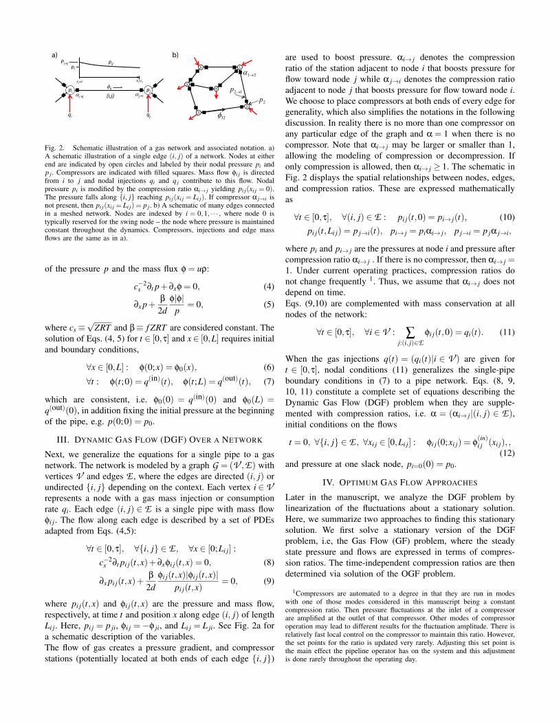
Fig. 2. Schematic illustration of a gas network and associated notation. a)A schematic illustration of a single edge (i, j) of a network. Nodes at eitherend are indicated by open circles and labeled by their nodal pressure pi andp j . Compressors are indicated with filled squares. Mass flow φi j is directedfrom i to j and nodal injections qi and q j contribute to this flow. Nodalpressure pi is modified by the compression ratio αi→ j yielding pi j(xi j = 0).The pressure falls along {i, j} reaching pi j(xi j = Li j). If compressor α j→i isnot present, then pi j(xi j = Li j) = p j . b) A schematic of many edges connectedin a meshed network. Nodes are indexed by i = 0,1, · · · , where node 0 istypically reserved for the swing node – the node where pressure is maintainedconstant throughout the dynamics. Compressors, injections and edge massflows are the same as in a).

of the pressure p and the mass flux φ = uρ:

c−2s ∂t p+∂xφ = 0, (4)

∂x p+β

2dφ|φ|

p= 0, (5)

where cs≡√

ZRT and β≡ f ZRT are considered constant. Thesolution of Eqs. (4, 5) for t ∈ [0,τ] and x∈ [0,L] requires initialand boundary conditions,

∀x ∈ [0,L] : φ(0;x) = φ0(x), (6)

∀t : φ(t;0) = q(in)(t), φ(t;L) = q(out)(t), (7)

which are consistent, i.e. φ0(0) = q(in)(0) and φ0(L) =q(out)(0), in addition fixing the initial pressure at the beginningof the pipe, e.g. p(0;0) = p0.

III. DYNAMIC GAS FLOW (DGF) OVER A NETWORK

Next, we generalize the equations for a single pipe to a gasnetwork. The network is modeled by a graph G = (V ,E) withvertices V and edges E , where the edges are directed (i, j) orundirected {i, j} depending on the context. Each vertex i ∈Vrepresents a node with a gas mass injection or consumptionrate qi. Each edge (i, j) ∈ E is a single pipe with mass flowφi j. The flow along each edge is described by a set of PDEsadapted from Eqs. (4,5):

∀t ∈ [0,τ], ∀{i, j} ∈ E , ∀x ∈ [0;Li j] :

c−2s ∂t pi j(t,x)+∂xφi j(t,x) = 0, (8)

∂x pi j(t,x)+β

2dφi j(t,x)|φi j(t,x)|

pi j(t,x)= 0, (9)

where pi j(t,x) and φi j(t,x) are the pressure and mass flow,respectively, at time t and position x along edge (i, j) of lengthLi j. Here, pi j = p ji, φi j =−φ ji, and Li j = L ji. See Fig. 2a fora schematic description of the variables.The flow of gas creates a pressure gradient, and compressorstations (potentially located at both ends of each edge {i, j})

are used to boost pressure. αi→ j denotes the compressionratio of the station adjacent to node i that boosts pressure forflow toward node j while α j→i denotes the compression ratioadjacent to node j that boosts pressure for flow toward node i.We choose to place compressors at both ends of every edge forgenerality, which also simplifies the notations in the followingdiscussion. In reality there is no more than one compressor onany particular edge of the graph and α = 1 when there is nocompressor. Note that αi→ j may be larger or smaller than 1,allowing the modeling of compression or decompression. Ifonly compression is allowed, then αi→ j ≥ 1. The schematic inFig. 2 displays the spatial relationships between nodes, edges,and compression ratios. These are expressed mathematicallyas

∀t ∈ [0,τ], ∀(i, j) ∈ E : pi j(t,0) = pi→ j(t), (10)pi j(t,Li j) = p j→i(t), pi→ j = piαi→ j, p j→i = p jα j→i,

where pi and pi→ j are the pressures at node i and pressure aftercompression ratio αi→ j . If there is no compressor, then αi→ j =1. Under current operating practices, compression ratios donot change frequently 1. Thus, we assume that αi→ j does notdepend on time.Eqs. (9,10) are complemented with mass conservation at allnodes of the network:

∀t ∈ [0,τ], ∀i ∈ V : ∑j:(i, j)∈E

φi j(t,0) = qi(t). (11)

When the gas injections q(t) = (qi(t)|i ∈ V ) are given fort ∈ [0,τ], nodal conditions (11) generalizes the single-pipeboundary conditions in (7) to a pipe network. Eqs. (8, 9,10, 11) constitute a complete set of equations describing theDynamic Gas Flow (DGF) problem when they are supple-mented with compression ratios, i.e. α = (αi→ j|(i, j) ∈ E),initial conditions on the flows

t = 0, ∀{i, j} ∈ E , ∀xi j ∈ [0,Li j] : φi j(0;xi j) = φ(in)i j (xi j), ,

(12)and pressure at one slack node, pi=0(0) = p0.

IV. OPTIMUM GAS FLOW APPROACHES

Later in the manuscript, we analyze the DGF problem bylinearization of the fluctuations about a stationary solution.Here, we summarize two approaches to finding this stationarysolution. We first solve a stationary version of the DGFproblem, i.e, the Gas Flow (GF) problem, where the steadystate pressure and flows are expressed in terms of compres-sion ratios. The time-independent compression ratios are thendetermined via solution of the OGF problem.

1Compressors are automated to a degree in that they are run in modeswith one of those modes considered in this manuscript being a constantcompression ratio. Then pressure fluctuations at the inlet of a compressorare amplified at the outlet of that compressor. Other modes of compressoroperation may lead to different results for the fluctuation amplitude. There isrelatively fast local control on the compressor to maintain this ratio. However,the set points for the ratio is updated very rarely. Adjusting this set point isthe main effect the pipeline operator has on the system and this adjustmentis done rarely throughout the operating day.

A. Stationary Gas Flow

In the GF problem, all input parameters (consump-tions/injections, compression ratios and the pressure at theslack bus) are constant in time. The total injection and con-sumption is balanced

∑i∈V

q(st)i = 0. (13)

The steady solution of Eq. (8) is uniform mass flow alongeach pipe in the network, ∀{i, j} : φi→ j = const. Substitutingthis result into Eq. (9) and integrating over space yields thealgebraic relationship between pressure at position x ∈ [0;Li j],compression, and (constant) flow through the pipe

∀(i, j) ∈ E : p(st)i→ j = p(st)

i αi→ j;

(p(st)i j (x))2 = (p(st)

i→ j)2− βx

dφ(st)i j |φ

(st)i j |. (14)

The GF problem has a unique solution provided the compres-sion ratios are known, and the GF solution in (14) is the basisfor many approaches to solving the OGF problem.

B. Optimum Gas Flow

The solution to the GF problem leaves the time-independentcompression ratios α unknown. These are chosen by thepipeline operators based on a combination of economic andoperational factors. Here, we describe two approaches forselecting the α. The first is a greedy algorithm that approxi-mates the current pipeline operations in the US. The guidingprinciple is that compressors are activated when the pressureprior to the next compressor drops below the acceptable lowerbound. When activated, a compressor is set to its maximumcompression ratio α. This algorithm is described in detailin [7]. The second approach is based on solutions to theoptimal gas flow (OGF) problem [14], [15], [16], [7]. Here,we summarize a Geometric Programming (GP) approach tosolving the OGF problem that minimizes the total compressorpower to move the gas.The total power used in pipeline gas compression (assumingthat the gas is ideal and compression is isentropic) is

∑(i, j)∈E

ci→ jφ(st)i j

ηi→ j

(max{αm

i→ j,1}−1), (15)

where ci→ j is a constant that depends on the compressor,m = (γ− 1)/γ where γ is the gas heat capacity ratio, andηi→ j is the efficiency factor of the compressor. It is importantto note that fluctuations caused by compressor consumptionare negligible when compared to gas loads. The term φ

(st)i j

denotes the directional mass flow for edge i, j, when the edgeis oriented from i to j. The OGF formulation assumes thatthe flow through the compressor is from i to j, i.e., φ

(st)i j > 0,

thus the direction of flow must be selected before hand. Fortree networks, the magnitude and direction of the flows arecomputed exactly apriori and do not depend on the choice ofcompression ratios. For an edge i, j, let Gi and G j be the two

disjoint graphs obtained by removing (i, j). The flows φ(st)i j are

computed as

φ(st)i j = ∑

i∈Gi

q(st)i =− ∑i∈G j

q(st)i . (16)

In networks with loops, flow direction is chosen using heuris-tics or through the introduction of binary variables [16].Using the cost function in Eq. (15), the OGF problem isformulated as

minα,p ∑

(i, j)∈E

ci→ jφi j

ηi→ j

(max{αm

i→ j,1}−1)

(17)

s.t. ∀(i, j) ∈ E : α2i→ j =

p2j +

βLi jdi j

φ2i j

p2i

, (18)

∀i ∈ V : 0≤ pi ≤ pi ≤ pi, (19)∀(i, j) ∈ E : αi→ j ≤ αi→ j ≤ αi→ j, (20)

where Eq. (18) is obtained from Eq. (14). The upper bound inEq. (19) represents engineering limits on pipes and the lowerbound represents contractual obligations. The upper and lowerbounds in Eq. (20) refer to maximum allowed compressionand decompression at each compressor. If decompression isnot allowed, αi→ j =1.There are a variety of methods for solving the OGF over trees,and in this paper, we use the geometric programming (GP)approach described in [7]. The GP approach relaxes the lowerbound αi→ j in Eq. (20), i.e. αi→ j =0. Under this relaxation,the OGF is transformed into a GP of the form

mint,β

log

(∑

(i, j)∈Edi jemti j

), ∀i ∈ V (21)

s.t. 2 log(pi)≤ βi ≤ 2log(pi) (22)

0≤ ti j ≤ log(αi j), (23)

log(

eβ j−βi−ti j +δ1i je−βi−ti j

)≤ 0, (24)

∀(i, j) ∈ E .

The transformed variables are related to the original ones viathe following equations

p2i = eβi , δ

1i j =

βLi j

di jφ

2i j. (25)

The OGF in Eqs. (21-24) is solved using convex optimization.When decompression is not allowed, αi→ j=1 in Eq. (20),we use a signomial programming (SP) method, which is aheuristic version of GP based on solving a sequence of convexprograms [7]. Here, we use SP to solve the OGF.

V. DIFFUSIVE JITTER OF PRESSURE FLUCTUATIONS

The main contribution of this manuscript builds on the so-lution of the OGF by introducing a model of stochasticgas consumption and the analysis of its effects on pressurefluctuations–diffusive jitter. Our approach linearizes the DGFequations (Eqs. 8,9) around a solution to the GF problem(augmented with compression ratios from the OGF or thegreedy compression scenario).

The linearized model captures the relationship between thefluctuating consumption and the fluctuating pressure. Asymp-totically, the accumulated changes in pressure provide an indi-cation of how fast the pressure will drift (the jitter) and exceedan operating limit in the absence of operator intervention. Asthe DGF solution drifts further from the original GF solution,the quality of the linearization degrades. However, we expectthat the linearized solution to the DGF remains a strongrelative indicator of how quickly a system will experienceproblems due to stochastic consumption.Formally, the stochastic consumption is defined by q(t) =q(st) + ξ(t) where the components of ξ(t) = (ξi(t)|i ∈ V )are time varying but relatively small in comparison to q(st).We assume a linearized solution of the DGF problem ofthe form p(t) = p(st)+ δp(t) and φ(t) = φ(st)+ δφ(t), wherethe respective corrections are small, i.e. |δp(t)| � p(st) and|δφ(t)| � φ(st). The linearized versions of Eqs. (8, 9, 10, 11)are

∀t ∈ [0,τ], ∀{i, j} ∈ E , ∀x ∈ [0;Li j] :

c−2s ∂tδpi j +∂xδφi j = 0, (26)

∂xδpi j +β

2d

(δφi j|φ

(st)i j |

p(st)i j

+

φ(st)i j |δφi j|

p(st)i j

−δpi jφ

(st)i j |φ

(st)i j |

(p(st)i j )2

)= 0, (27)

∀t ∈ [0,τ], ∀(i, j) ∈ E :δpi→ j = δpiαi→ j, (28)δpi j(t,0) = δpi→ j(t), δpi j(t,Li j) = δp j→i(t), (29)

∀t ∈ [0,τ], ∀i ∈ V : ∑j:(i, j)∈E

δφi j(t,0) = ξi(t). (30)

We seek asymptotic solutions to the PDE of Eqs. (26, 27,28,29,30), where asymptotic implies finding solutions fortime τ longer than the correlation time of the fluctuationconsumption ξ. In addition, we seek solutions of Eqs. (26,27,28,29,30) that connect the nodal quantities by algebraicrelationships thereby eliminating the complexity of the orginalPDE.The solution approach is an extension of the work in [8].Following [8], we solve Eqs. (26, 27) for each pipe usinga proposed solution of the form

δpi j = ai j(t)Zi j(x)+bi j(t,x), (31)

where the ai j(t) depend on time. In [8], it was argued thatthe ai j(t)Zi j(x) term represents the asymptotic contributionto the gas pressure fluctuations that grows in time. In con-trast, bi j(t,x) represents smaller contributions to the pressurefluctuations that do not grow in time. Here, we focus on thecontribution from the ai j(t)Zi j(x) term which is asymptoticallydominant at long times.2

2Bounds for the second term are derived and solved using inhomogeneouslinear equations for bi j .

Substitution of proposed solution (31) into Eqs. (26, 27) yieldsan equation for Zi j, i.e.

∂xZi j−β

2d

φ(st)i j |φ

(st)i j |

(p(st)i j )2

Zi j = 0, (32)

where Zi j(x) counts x from node i. The integration of Eq. (32)over the spatial dependence of the stationary profile (14),yields

Zi j(x) =p(st)

i→ j + p(st)j→i

2p(st)i j (x)

, (33)

where the normalization constant is chosen to guarantee,∫ L0 Zi j(x)dx/L = 1.

We solve for the time-dependent factor ai j(t) by substitutingδpi j ∼ ai j(t)Zi j(x) into Eq. (26) and integrating the result overthe entire spatial extent of the pipe {i, j} yielding

ai j(t) = c2s

∫ t

0dt ′(δφi j(t ′,0)−δφi j(t ′,L)

). (34)

In the asymptotic limit where δpi j ∼ ai j(t)Zi j(x) for everypipe (graph edge), Eqs. (29) can only be satisfied if the ai j(t)have the same functional dependence on time, i.e.,

∀{i, j} ∈ E : ai j(t) = a(t)ci j, (35)

where ci j = c ji is an edge specific constant.To compute the global time-dependent factor a(t) we sum themass conservation equation over all the nodes of the graph

∑i∈V

ξi = ∑{i, j}∈E

(δφi j(t,0)−δφi j(t,Li j)) , (36)

integrate over time and define

Ξ(t) .=

∫ t

0dt ′ ∑

i∈Vξi(t ′), (37)

and finally sum Eq. (35) overall edges:

a(t) =c2

s Ξ(t)∑{i, j}∈E ci j

. (38)

Therefore, ∀t, ∀{i, j} ∈ E , x ∈ [0,Li j] :

δpi j(t,x)≈c2

s Ξ(t)∑{i, j}∈E ci j

ci jZi j(x). (39)

The unknown edge constants ci j are derived by substitutingEqs. (39) into Eqs. (28, 35) yielding

∀i, ∀ j,k s.t. (i, j),(i,k) ∈ E :ci jZi j(0)

αi→ j=

cikZik(0)αi→k

. (40)

Eqs. (39, 40, 33) express the complete asymptotic (zero mode)solution of the DGF problem.Finally, we make several observations to connect the solutionfor the pressure fluctuations in Eqs. (39, 40, 33) to a prob-ability distribution over the pressure fluctuations. First, therandom gas load fluctuations ξi(t) are zero-mean, temporarilyhomogeneous, and relatively short correlated in both time (thecorrelation time is less than τ) and space (the correlation length

is less than the spatial extent of the network). Second, thefluctuations of δpi j in Eq. (39) are given by a time-integraland spatial-sum of the fluctuations. According to the LargeDeviation theory, these observations imply that the pressurefluctuations form a Gaussian random process which jittersdiffusively in time. Specifically, the Probability DistributionFunction (PDF) of δpi j(t,x) is

P (δpi j(t,x) = δ)→ (2πtDi j(x))−1/2 exp

(− δ2

2tDi j(x)

), (41)

Di j =

(c2

s ci jZi j(x)∑{k,l}∈E ckl

)2⟨(∑

n∈Vξn(t ′)

)2⟩, (42)

where the correlation function on the right-hand-side does notdepend on t ′ due to assumption of the statistical homogeneityof ξ.

VI. NUMERICAL EXPERIMENTS

Inspection of Eq. (42) shows that the variance of the pressurefluctuations as a function of position in the network is relatedto the coefficients Di j(x), referred to collectively as D. Highervalues of D correspond to larger pressure fluctuations andhigher likelihood of the pressure violating an engineering orcontractual limit. By analogy with related physical processes,the coefficients D are similar to a diffusion coefficient, and werefer them this way in the remainder of the manuscript. Theorigins of D are primarily twofold. Once the gas consumptionsand injections are fixed, the spatial dependence of D arisesfrom the particular stationary solution of pressures, flows, andcompression ratios through the Zi j(x). The magnitude of D isalso related to the average global strength of the consumptionfluctuations 〈(∑n∈V ξn(t ′))

2〉.We apply the results described above to the Transco pipelineshown schematically in Fig. 1. We use data for the total con-sumption at each node over a 24-hour period from December29, 2012 to fix the forecasted consumption for the stationaryGF solution. These data represent relatively stressed operationsfor the Transco pipeline. The Transco pipeline has a smallnumber of loops, which we partition to create a tree topology[7] that is very nearly linear but with a few small branches.We resolve these branches in the solution of the GF (or OGF)problem, however, when analyzing the pressure fluctuations,we aggregate these short branches to nodal consumptions andonly analyze the fluctuations as a function of distance alongthe mainline.The Transco operational data does not include informationon the deviations of the gas flows from their average orscheduled values. Instead, we estimate the global mean-squareconsumption fluctuations as⟨(

∑n∈V

ξn(t ′)

)2⟩≈(

φ0

3

)2

∗N. (43)

Here, φ0 ≈ 20 kg/s is a typical average consumption for anode in the Transco pipeline, and N ≈ 70 is the numberof consumption nodes, e.g. city-gates or power plants. This

estimate of the gas consumption fluctuations assumes thatthe fluctuations at neighboring nodes are uncorrelated. Ifthese neighboring nodes are gas-fired turbine generators thatare both being used to balance renewable fluctuations, theassumption of independence may lead to an underestimationin Eq. (43).For presentation purposes, it is convenient to find a suitablenormalization for D. Motivated by Eqs.(41,43), we normalizeD by

D0 ≈( p0

3

)2/t0

where p0 = 800 psi ≈ 5.5 ∗ 106 Pa is the upper bound onallowed pressure in the pipes and t0 = 15 min ≈ 103s is arepresentative time period where we expect the developedtheory to work well.We consider the base case of December 29th, 2012 andseveral modifications of this base case to investigate theeffects of changing operations. Fig. 3 displays D as a functionof location along the mainline for two different stationarysolutions for the base case—the OGF solution described inSection IV and the greedy algorithm from [7]. For a charac-teristic time of 15 min ≈ 103s, D/Do = 1 corresponds to avariance in pressure fluctuations of (266 psi)2. Pressures inthe Transco Pipeline range between 500 psi and 800 psi, sothe pressure fluctuation standard deviation is 33−53% of thepressures in the pipeline for D/Do = 1. The same characteristictime and D/Do = 0.1 yields a variance of (84 psi)2 whichgives pressure fluctuation standard deviations of 10−16% ofpipeline pressures. Since the pressure variance grows linearlyin time, often over several 15 min intervals, these fluctuationscan quickly grow to exceed pressure bounds without properintervention. As the plots show, most pressure fluctuations areabove D/Do = 0.1 throughout the pipeline, and therefore thefluctuations are of concern in any regions of pipeline where thepressure is near its upper or lower bound. The two solutionsdisplay similarities. Both show a build up of D from milepost800 nearer to the Gulf of Mexico, a peak at milepost 1771 nearNew York and New Jersey, and a decay to a smaller value atmilepost 2000 near the injection point for the Marcellus Shalein Pennsylvania.The spatial variation of D is due to Zi j(x), and the generalshape of D can be understood by revisiting Eq. 32. Theform of this equation suggest exponential growth or decayof Zi j(x) depending on the orientation of φi j. The flow fromthe Gulf to the New York/New Jersey area is unidirectionalcreating the growth of D observed in Fig. 3. However, thelarge loads in the New York/New Jersey area combined withthe offsetting injections from from the Marcellus Shale createsa flow reversal and an exponential decay of Zi j (and thereforeof D). The peak in D is connected to the point of flow reversal.The solution in Fig. 3 displays more structure than simpleexponential growth and decay for several reasons. First, themass flow rates φi j depend on location. However, perhapsmore important are the discontinuities in D. These occur atcompressor stations and are due to the discontinuities in p(st)

at these locations.The global behavior of the OGF solution and the greedyalgorithm Fig. 3 is similar because the differences in thecompression ratios in the stationary solution does not affect themass flow rates. However, it does affect the spatial dependenceof pressure which can lead to the substantial local differencesobserved in Fig. 3. For example, between mileposts 1400 and1700, D is much lower for the greedy algorithm comparedto the OGF. However, the deployment of a compressor nearmilepost 1700 in the greedy algorithm leads to a large jumpin D, a larger peak in pressure fluctuations, and a greaterchance for violation of an engineering or contractual pressurelimit. For this one example, this difference would seem tosuggest that the OGF solution is less susceptible to pressurefluctuations. However, we note that the expected magnitude ofthe pressure fluctuations is not taken into account in either thegreedy algorithm or the OGF.What these results do suggest is that the deployment ofcompressors in the stationary solution can have a significantimpact on the expected pressure fluctuations, and that it ispossible to formulate a a compressor dispatch optimizationthat balances the risk of such fluctuations against other desiredoperational properties, e.g. cost. The simple algebraic form ofthe probability of such large fluctuations in Eqs. (41,42) areconvenient for incorporation into such formulations.To determine the effect of overall consumption and injectionon D, we uniformly scaled the base case consumptions andinjections by a constant factor—a scaling that preserves thebalance of consumptions and injections required for the exis-tence of a stationary solution. Figure 4 displays the results forD computed using the OGF stationary solutions. The stationarysolutions show small local differences in D caused by thedeployment of compression. However, the major impact stemsfrom the increase (or decrease) in mass flows. The uniformscaling does not affect the location of the flow reversal, sothe peak in D appears at the same place. However, the larger(smaller) flows lead to faster (slower) growth rates for Zi j (seeEq. 32) and an overall higher (lower) peak in D.In recent years the Marcellus Shale has become a largesupplier of gas, and its injection capability is expected toincrease [17]. To model the effect of this expansion we scaledall injections from the Marcellus Shale by a constant factor andremoved a corresponding amount of gas from the injectionsat the Gulf to preserve the global balance of consumptionand injection. Fig. 5 displays the results for D along theTransco pipeline for the OGF solution. Although the injectionfrom the Marcellus is increased, the major gas load centersin New York and New Jersey keep the flow reversal point,and therefore the peak in D, pinned at more or less the samelocation. Larger Marcellus injections show slightly lower peakamplitudes of D indicating that, as gas injections are shiftedfrom the Gulf to the Marcellus Shale, the reliability of pipelineoperations is improved. We conjecture that this change is dueto moving the source of gas injections closer to the major loadcenters. However, we again note that the OGF methods usedto find the stationary solution do not account for the expected

600 800 1000 1200 1400 1600 1800 2000Milepost [miles]

0.0

0.2

0.4

0.6

0.8

1.0

1.2

D/Do

Signomial ProgramGreedy Algorithm

Fig. 3. Diffusion coefficient as a function of distance along the Transcomainline with stationary solutions given by OGF and the greedy algorithm.Both show a peak at milepost 1771, but the magnitude of this peak is muchhigher for the greedy algorithm than the OGF, indicating larger pressurefluctuations for the greedy algorithm.

pressure fluctuations and their inclusion will likely lead to amodification of these results.Although scaling overall consumption and Marcellus supplyare directly relevant to operators and planners, they do notexhibit a shift in the location of the peak in D or the appearanceof multiple local maxima. To study these possibilities, wenext imposed some less realistic changes. In particular, theloads in New York are shifted to points closer to the Gulf andMarcellus Shale, but the New Jersey loads were left unaffected.Fig. 6 displays the impact of this shift on D computed usingstationary solutions from the OGF and the greedy algorithm.Since the large load in New Jersey remains, milepost 1771 isstill a position of flow reversal and a, now minor, maximumof D. However, the redistribution of load leads to a newglobal maximum near milepost 1319—a large load in NorthCarolina. Although the location of maximum fluctuations hasbeen relocated, the maximum of D is much reduced by movingthe loads closer to the gas injections.The previous example showed the appearance of a new globalmaximum, as well as several small local maxima, but the orig-inal local maximum remained. To remove it, we shifted NewJersey’s load to points closer to the Gulf and the MarcellusShale, as shown in Fig. 7. This successfully removes the localmaximum at milepost 1771 while leaving the global maximumat milepost 1319. In this case the jitter (diffusion coefficient)of the greedy algorithm and OGF are comparable, with OGFjitter greater before milepost 1319 and greedy greater aftermilepost 1319.

VII. CONCLUSIONS AND FUTURE WORK

We have focused the analysis on the coupling between naturalgas networks and electric networks at the time scale of intra-day natural gas markets. The coupling at this time scale isexpected to become tighter because of several factors: the

600 800 1000 1200 1400 1600 1800 2000Milepost [miles]

0.0

0.1

0.2

0.3

0.4

0.5

0.6

0.7

0.8

0.9D/D

o

Base Consumption1.1*Base Consumption0.9*Base Consumption

Fig. 4. Diffusion coefficient as a function of distance along the Transcomainline with stationary solutions given by the OGF with global consumptionand injection scaled by a uniform factor. All show a peak at milepost 1771,but higher scaling factors have higher magnitudes at their peaks, indicatinglarger pressure fluctuations for larger system loads.

600 800 1000 1200 1400 1600 1800 2000Milepost [miles]

0.0

0.2

0.4

0.6

0.8

1.0

D/D

o

Base Marcellus Shale Injection1.2*Base Shale Injection0.8*Base Shale Injection

Fig. 5. Diffusion coefficient as a function of distance along the Transcomainline with stationary solutions given by the OGF with Marcellus Shaleinjections scaled by a factor and the corresponding amount of injectionsremoved from the Gulf. All show a peak at milepost 1771, but higher scalingfactors have slightly lower magnitude at the peak, indicating smaller pressurefluctations. Higher scaling factors also have much lower magnitudes in theMarcellus Shale, indicating smaller pressure fluctuations when injections areshifted from the Gulf to the Marcellus Shale.

retirement of coal and fuel oil-fired generation in favor ofnatural gas-fired generation because of environmental concernsand the increased availability and low cost of natural gas andthe ability of gas-fired generation to respond quickly to thevariability of renewable generation. Although gas pipelineshave the ability store gas in the form of increased pressurein the piepline, i.e. linepack, this storage is limited. In thefuture, linepack will be increasingly exercised as more gas-fired generation is used to balance increasing amounts of windgeneration. Larger swings in gas pipeline pressure (linepack)

600 800 1000 1200 1400 1600 1800 2000Milepost [miles]

0.10

0.15

0.20

0.25

0.30

0.35

D/Do

Signomial ProgramGreedy Algorithm

Fig. 6. Diffusion coefficient as a function of distance along the Transcomainline with load redistributed from the large load in New York to the Gulfand Marcellus Shale, leaving the large load in New Jersey unaltered. Thiscauses the appearance of a new global maximum at milepost 1319 which isthe location of a large load in North Carolina. Since the New Jersey load wasnot redistributed, a local maximum remains at milepost 1771.

600 800 1000 1200 1400 1600 1800 2000Milepost [miles]

0.10

0.15

0.20

0.25

0.30

0.35

D/Do

Signomial ProgramGreedy Algorithm

Fig. 7. Diffusion coefficient as a function of distance along the Transcomainline with load redistributed from the large loads in New York and NewJersey closer to the Gulf and Marcellus Shale. The global maximum atmilepost 1319 remains, but the local maximum at milepost 1771 dissappearssince the large load has been removed from this area.

affect the ability of the pipeline to deliver gas to the generators,creating reliability implications that cascaded across these twoinfrastructures.In this initial work, we have assessed the impact of fluctuatingconsumption by gas-generators on pipeline pressure. We startby splitting the gas flow equations for pipelines into two parts.The first is a stationary part that is time-independent andreflects the gas flows scheduled by the gas markets and gascompressor deployment determined by the pipeline operator.The second is a representation of the fluctuations around thescheduled flows created by linearizing the gas flow equationsabout the scheduled flows and compressor operations. Fromthis linearized model, we can predict the probability that aset of stochastic gas loads will cause the pipeline pressure toviolate an engineering or contractual pressure limit and create

a reliability concern for the pipeline operator or the electricalgrid operator. By making assumptions about the nature of thegas consumption fluctuations, this probability can be expressedin an algebraic form that is convenient for integration intoa gas flow/gas compressor optimization problem where theprobability can be a constraint or part of the objective to limitthe likelihood of a pipeline reliability issue.We applied the theoretic results to a realistic model based onthe Transco pipeline. Our computational experiments with theTransco model revealed the following interesting observations.First, the probability of large pressure fluctuations is highestat locations in the pipeline where the gas flow experiences areversal (in and around the New York/New Jersey area for theTransco pipeline). Second, increasing the stress on the pipelineby increasing gas flow rates leads to higher probabilities oflarge pressure fluctuations. Third, rearranging pipeline flows,e.g. by increasing purchases from the Marcellus Shale at theexpense of gas from the Gulf, can decrease the probability oflarge pressure fluctuations by moving the gas sources closerto the gas loads.The results of this paper suggest a number of interestingdirections for future research.• The linearization and asymptotic assumptions described

here need to be validated against direct dynamic (tran-sient) simulations of gas flows in variety of situations.Most existing work on such validations [18], [12], [19],[20], [21], [22] uses single pipe models. The challengeis to develop fast computational algorithms for transientproblems with mixed (initial and boundary) conditionsover large and loopy gas networks.

• Our dynamic method applies to gas networks with loops,back flows, bi-directional compression and other compli-cations. We will extend the experimental study to othercurrent and planned networks in the U.S. and Europe.

• Extending the probabilistic risk framework to the compli-cations mentioned above requires extending the methodsof [7] to create efficient optimization algorithms for gasnetworks with loops.

• Compressor positions are assumed fixed by the OGFand greedy solution methods presented here. However,compressor position has a significant effect on pressurefluctuations in its vicinity. A future direction will beto formulate a compressor dispatch scheme and use itto analyze the effect of varying compressor position onpressure fluctuations near the compressors.

• Incorporation of the probabilistic risk measures into OGFformulations to directly account for this risk. A promisingdirection is the chance constrained methodology devel-oped in [23].

• This work suggests a new mathematical, statistical andcomputational foundations necessary to address the com-prehensive strategic problems of re-organizing the exist-ing system of energy trading (in the U.S. and elsewhere).Such a reorganization is required to reduce inefficienciesin how power and gas markets interact [1], [2], [24].

• It is not realistic to expect (at least not in US) that

gas and power markets will merge in the near future.However, it is important to account for effects of mutualdependencies. In particular, incorporating effects of gaspressure fluctuations and uncertainty into planning andoperations of power systems with significant penetrationsof renewables and with gas turbines involved in balancingthe renewable fluctuations is a very promising futuredirection for research. On the other hand it is as importantto account for the effect of ramps in gas consumptions atgenerators on the gas flow optimization.

REFERENCES

[1] “The Future of Natural Gas:MIT Energy Initiative, http://mitei.mit.edu/system/files/NaturalGas Report.pdf,” 2010.

[2] “Growing concerns, possible solutions: The interdependency ofnatural gas and electricity systems, http://mitei.mit.edu/system/files/2014-MITEI-Report-Growing-Concerns-Possible-Solutions.pdf,” 2014.

[3] “ISO New England: Adressing Gas Dependence, http://www.iso-ne.com/committees/comm wkgrps/strategic planningdiscussion/materials/natural-gas-white-paper-draft-july-2012.pdf,”2012.

[4] “Renewable portfolio standards in the states: Balancing goals and im-plementation strategies, http://www.nrel.gov/docs/fy08osti/41409.pdf,”2007.

[5] “Levelized cost of electricity renewable energy tech-nologies, http://www.ise.fraunhofer.de/en/publications/veroeffentlichungen-pdf-dateien-en/studien-und-konzeptpapiere/study-levelized-cost-of-electricity-renewable-energies.pdf,” 2013.

[6] T. J. Considine, R. Watson, and S. Blumsack, “The Economic Impactsof the Pennsylvania Marcellus Shale Natural gas play: An update,” 2010.

[7] S. Misra, M. W. Fisher, S. Backhaus, R. Bent, M. Chertkov, andF. Pan, “Optimal compression in natural gas networks: a geometricprogramming approach,” IEEE Transactions on Control of NetworkSystems (CONES), 2015.

[8] M. Chertkov, V. Lebedev, and S. Backhaus, “Cascading of Fluctuationsin Interdependent Energy Infrastructures: Gas-Grid Coupling,” ArXiv e-prints, Nov. 2014.

[9] CRANE, “Flow of fluids: Through valves, fittings and pipe,” CraneCompany, New York, Technical paper 410M, 1982.

[10] S. Mokhatab, W. A. Poe, and J. G. Speight, Handbook of Natural GasTransmission and Processing. Houston: Gulf Professional Publishing,2006.

[11] A. Osiadacz, Simulation and analysis of gas networks. GulfPub. Co., 1987. [Online]. Available: http://books.google.com/books?id=cMxTAAAAMAAJ

[12] A. Thorley and C. Tiley, “Unsteady and transient flow of compressiblefluids in pipelinesa review of theoretical and some experimentalstudies,” International Journal of Heat and Fluid Flow, vol. 8, no. 1,pp. 3 – 15, 1987. [Online]. Available: http://www.sciencedirect.com/science/article/pii/0142727X87900440

[13] S. A. Sardanashvili, Computational Techniques and Algorithms (PipelineGas Transmission) [in Russian]. FSUE Oil and Gaz, I.M. Gubkin,Russian State University of Oil and Gas, 2005.

[14] P. Wong and R. Larson, “Optimization of natural-gas pipeline systemsvia dynamic programming,” Automatic Control, IEEE Transactions on,vol. 13, no. 5, pp. 475–481, 1968.

[15] S. Wu, R. Ros-Mercado, E. Boyd, and L. Scott, “Model relaxationsfor the fuel cost minimization of steady-state gas pipeline networks,”Mathematical and Computer Modelling, vol. 31, no. 23, pp. 197 – 220,2000. [Online]. Available: http://www.sciencedirect.com/science/article/pii/S0895717799002320

[16] C. Borraz-Sanchez, “Optimization methods for pipeline transportation ofnatural gas,” Ph.D. dissertation, Department of Informatics, Universityof Bergen, Norway, October 2010.

[17] “2013 special reliability assessment: Accommodating an increaseddependence on natural gas for electric power phase ii: A vulner-ability and scenario assessment for the north american bulk powersystem, http://www.nerc.com/pa/RAPA/ra/Reliability%20Assessments%20DL/NERC PhaseII FINAL.pdf,” 2013.

[18] A. Osiadacz, “Simulation of transient gas flows in networks,”International Journal for Numerical Methods in Fluids, vol. 4, no. 1,pp. 13–24, 1984. [Online]. Available: http://dx.doi.org/10.1002/fld.1650040103

[19] W. Tao and H. Ti, “Transient analysis of gas pipeline network,”Chemical Engineering Journal, vol. 69, no. 1, pp. 47 – 52,1998. [Online]. Available: http://www.sciencedirect.com/science/article/pii/S1385894797001095

[20] J. Zhou and M. A. Adewumi, “Simulation of transients innatural gas pipelines using hybrid tvd schemes,” InternationalJournal for Numerical Methods in Fluids, vol. 32, no. 4, pp.407–437, 2000. [Online]. Available: http://dx.doi.org/10.1002/(SICI)1097-0363(20000229)32:4〈407::AID-FLD945〉3.0.CO;2-9

[21] C. Dorao and M. Fernandino, “Simulation of transients in naturalgas pipelines,” Journal of Natural Gas Science and Engineering,vol. 3, no. 1, pp. 349 – 355, 2011. [Online]. Available: http://www.sciencedirect.com/science/article/pii/S1875510011000059

[22] R. Alamian, M. Behbahani-Nejad, and A. Ghanbarzadeh, “A statespace model for transient flow simulation in natural gas pipelines,”Journal of Natural Gas Science and Engineering, vol. 9, no. 0, pp. 51– 59, 2012. [Online]. Available: http://www.sciencedirect.com/science/article/pii/S1875510012000662

[23] D. Bienstock, M. Chertkov, and S. Harnett, “Chance-constrainedoptimal power flow: Risk-aware network control under uncertainty,”SIAM Review, vol. 56, no. 3, pp. 461–495, 2014. [Online]. Available:http://dx.doi.org/10.1137/130910312

[24] R. Tabors and S. Adamson, “Measurement of energy market inefficien-cies in the coordination of natural gas amp;amp; power,” in SystemSciences (HICSS), 2014 47th Hawaii International Conference on, Jan2014, pp. 2335–2343.