NOTICE: The author has granted a nonexclusive license allowing Library and Archives Canada to reproduce, publish, archive, preserve, conserve, communicate to the public by telecommunication or on the Internet, loan, distribute and sell theses worldwide, for commercial or noncommercial purposes, in microform, paper, electronic and/or any other formats.
AVIS: L'auteur a accorde une licence non exclusive permettant a la Bibliotheque et Archives Canada de reproduire, publier, archiver, sauvegarder, conserver, transmettre au public par telecommunication ou par Plntemet, prefer, distribuer et vendre des theses partout dans le monde, a des fins commerciales ou autres, sur support microforme, papier, electronique et/ou autres formats.
The author retains copyright ownership and moral rights in this thesis. Neither the thesis nor substantial extracts from it may be printed or otherwise reproduced without the author's permission.
L'auteur conserve la propriete du droit d'auteur et des droits moraux qui protege cette these. Ni la these ni des extraits substantiels de celle-ci ne doivent etre imprimes ou autrement reproduits sans son autorisation.
In compliance with the Canadian Privacy Act some supporting forms may have been removed from this thesis.
Conformement a la loi canadienne sur la protection de la vie privee, quelques formulaires secondaires ont ete enleves de cette these.
While these forms may be included in the document page count, their removal does not represent any loss of content from the thesis.
Canada
Bien que ces formulaires aient inclus dans la pagination, il n'y aura aucun contenu manquant.
ABSTRACT
Pressure Loss Modeling of Non-Symmetric Gas Turbine Exhaust Ducts using CFD
Steven Farber
In typical gas turbine applications, combustion gases that are discharged from the turbine
are exhausted into the atmosphere in a direction that is sometimes different from that of the
inlet. In such cases, the design of efficient exhaust ducts is a challenging task particularly
when the exhaust gases are also swirling. Designers are in need for a tool today that can
guide them in assessing qualitatively and quantitatively the different flow physics in these
exhaust ducts so as to produce efficient designs.
In this thesis, a parametric Computational Fluid Dynamics (CFD) based study was
carried out on non-symmetric gas turbine exhaust ducts where the effects of geometry and
inlet aerodynamic conditions were examined. The results of the numerical analysis were
used to develop a total pressure loss model.
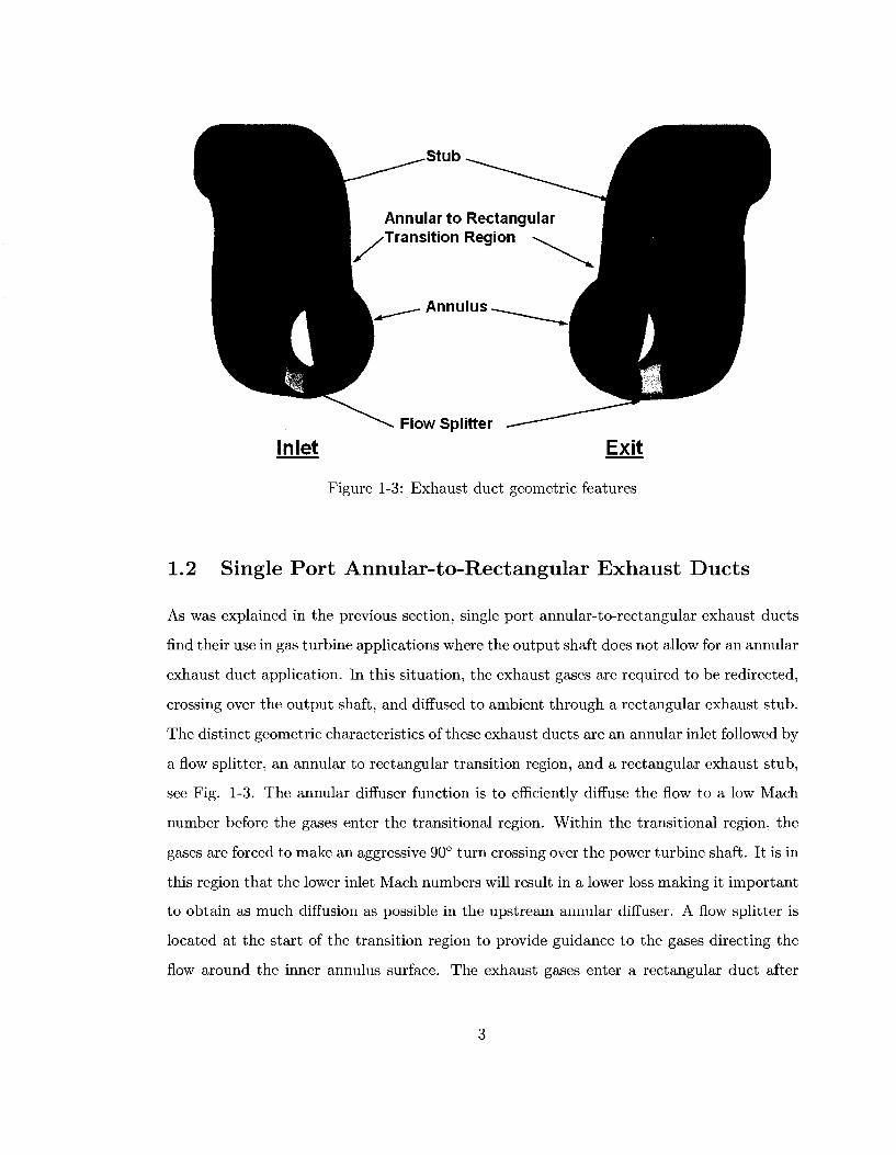
These exhaust ducts comprise an annular inlet, a flow splitter, an annular to rectangular
transition region, and an exhaust stub. The duct geometry, which is a three-dimensional
complex one, is approximated with a five-parameter model, which was coupled with a design
of experiment method to generate a relatively small number of exhaust ducts. The flow in
these ducts was simulated using CFD for different values of inlet swirl and aerodynamic
blockage and the numerical results were reviewed so as to assess the effects of the geometric
and aerodynamic parameters on the total pressure loss in the exhaust duct. These flow
simulations were used as a data base to generate a total pressure loss model that designers
can use as a tool to build more efficient non-symmetric gas turbine exhaust ducts. The
resulting correlation has demonstrated satisfactory agreement with the CFD-based data.
m
Acknowledgments
I would like to first thank my supervisor Prof. W.S. Ghaly and Co-supervisor Ed Vlasic
for their guidance and suggestions on this project.
Thanks also go to the following people and organizations without which this work would
not have been possibe:
To Pratt & Whitney Canada for their financial and technical support, especially Remo
Marini and Mark Cunningham.
To the Natural Sciences and Engineering Research Council of Canada (NSERC) for
financial support.
IV
Contents
1 Introduction 1
1.1 Background 1
1.2 Single Port Annular-to-Rectangular Exhaust Ducts 3
1.3 Contribution and Scope of the Present Study 4
2 Theory and Literature Review 6
2.1 Diffuser Performance 6
2.1.1 Static Pressure Recovery Coefficient 6
2.1.2 Diffuser Effectiveness 7
2.1.3 Total Pressure Loss Coefficient 7
2.2 Conical Diffusers 7
2.2.1 Geometry 7
2.2.2 Swirl 8
2.2.3 Aerodynamic Blockage 9
2.3 Annular Diffusers 11
2.3.1 Swirl 14
2.3.2 Aerodynamic Blockage 19
2.4 Past Research Contributions 21
2.4.1 Loka et al 21
2.4.2 Cunningham 24
3 Design of Experiment 30
3.1 Geometric Design Space 30
v
3.1.1 Equivalent Cone Diffusion Angle 31
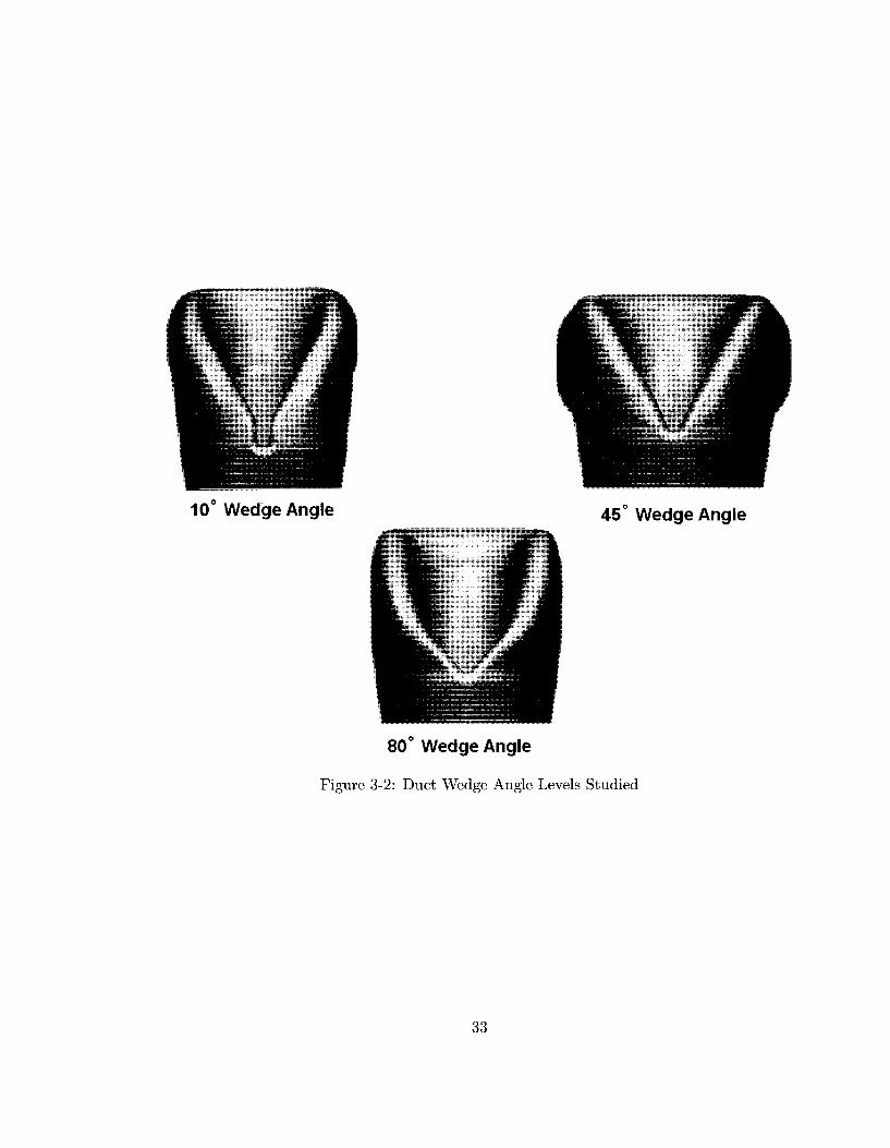
3.1.2 Flow Splitter Wedge Angle 31
3.1.3 Gas Path Aspect Ratio 34
3.1.4 Annular to Rectangular Transition Region 35
3.1.5 Exhaust Stubs 36
3.2 Aerodynamic Design Space 38
3.2.1 Swirl 38
3.2.2 Inlet Boundary Layer Blockage 40
3.3 Full Factorial Design 40
3.4 Taguchi Design 43
3.4.1 Assumption 43
3.4.2 Interactions 43
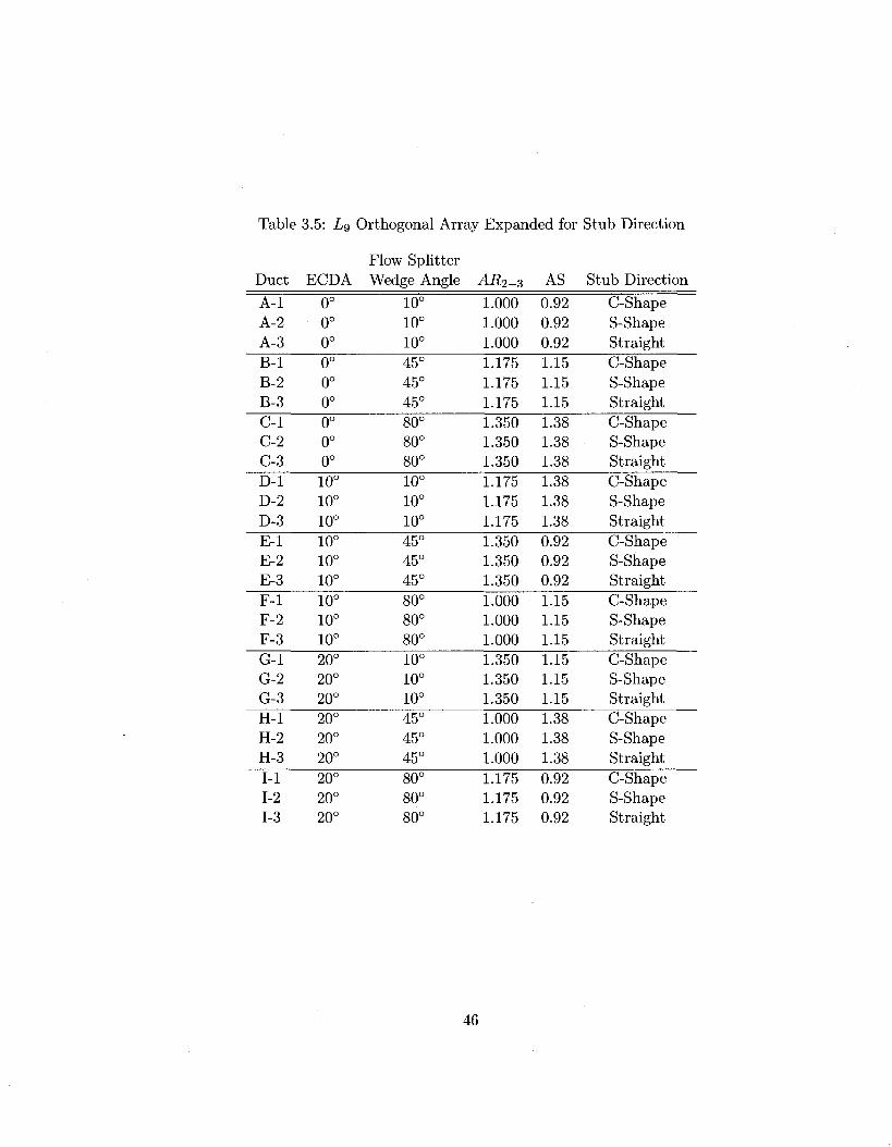
3.4.3 Selecting an Orthogonal Array 44
4 Geometry Synthesis 47
4.1 Equivalent Cone Diffusion Angle 49
4.2 Gas Path 51
4.3 Gas Path Aspect Ratio 51
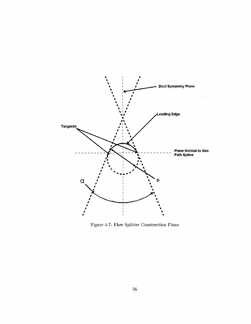
4.4 Flow Splitter Leading Edge 51
4.5 Flow Splitter Wedge Angle 54
4.6 Duct Exit Cross-Section 54
4.7 Annular to Rectangular Transition Region 57
4.8 Plenum 59
5 Computational Study 62
5.1 Data Reduction 62
5.2 Pressure-Velocity Coupling 63
5.3 Advection Scheme 63
5.4 Turbulence Modelling 64
5.4.1 k - e 64
5.4.2 SST 64
VI
5.5 Computational Domain 65
5.5.1 Boundary Conditions 66
5.5.2 Grid Structure 68
5.5.3 Grid Study 72
6 CFD-Based Parametric Study 78
6.1 Effect of Swirl 79
6.2 Effect of Stub Direction 85
6.3 Effect of ECDA 87
6.4 Effect of Wedge Angle 89
6.5 Effect of Aspect Ratio and Area Ratio in the Annular to Rectangular Tran
sition Region 92
6.6 Effect of Inlet Boundary Layer Blockage 96
7 Correlation of the Total to Total Pressure Loss 99
7.1 Japikse Correlation of Annular Diffusers 100
7.2 Correlation of the CFD Results 104
8 Conclusion and Recommendation 111
8.1 Conclusion I l l
8.2 Recommendation 112
Bibliography 114
vn
List of Figures
1-1 Pratt and Whitney PW200 engine 2
1-2 Pratt and Whitney PT6 engine 2
1-3 Exhaust duct geometric features 3
2-1 Conical diffuser presented with dimensional parameters 8
2-2 Conical diffuser performance chart based on data from Cockrell and Mark-
land (Bt « .20) 9
2-3 Conical diffuser performance chart from McDonald and Fox 10
2-4 Diffuser performance coefficient as a function of area ratio for (a) axial inlet
flow (b) swirling inlet flow 11
2-5 Radial distributions of total and static pressures at the inlet section . . . . 12
2-6 Variation of total pressure along stream surfaces of revolution 12
2-7 Maximum Pressure Recovery of Conical and Square Diffusers - Mth = 0.8 . 13
2-8 Variation of the total pressure loss coefficient with entrance length (X/D) for
a 5°; a) Reynolds number 1 x 10⁵, b) Reynolds number 4 x 10⁵ 13
2-9 Conical diffuser loss map using Sharan's data 14
2-10 Exit discharge area ratio for conical diffusers on Cp* (based on data from
| l l | < ' / T """—-Stal* irewc ilsnj ft* «n(er" — State pmswt ai»r.} the *8ll
(a )
2
0>}
3 z/D,
Figure 2-6: Variation of total pressure along stream surfaces of revolution [10]
12
*
8.3
Figure 2-7: Maximum Pressure Recovery of Conical and Square Diffusers - Mth = 0.8 [11]
0,4
0.3
o.2r. /
0.1
**\
o AR* 1.5 «4S = 2,5 „ 4ft* 3.5 n/W»S.O
0
SA-'-v<V * " ' tx_„.
^ ^•Y /
0 20 40 60 80 100 120 140 160
mo (a)
0.4 s < j 0.3[•
0.2!
0.1
0
o API- 1.5
<, 4fl«3.S n WJ«5.0
=:qr:i=^—-^
0 20 40 60 80 Too' 120 140 160 XID
(b)
Figure 2-8: Variation of the total pressure loss coefficient with entrance length (X/D) for a 5°; a) Reynolds number 1 x 10⁵, b) Reynolds number 4 x 10⁵ [12]
13
1
\
K° m 0
— ~ r —
*
» X
Symbol 0
E) f
m
r i -AR X/O Inlet 2.5
a.s
S.O
5.0
\
10-150
10-150
TO-150
10-150
—J
i Ha
1X10S
snias •
w o 5
6x10 B "
-
0.5 0.6 0,7 0.8 0.3 1.0
Figure 2-9: Conical diffuser loss map using Sharan's data [12]
Curved wall diffusers, which include axial to radial diffusers, are more complicated to
describe requiring their own derivation of L/h and AR specific to each shape.
Some of the first used annular diffuser maps produced by Sovran and Klomp [1] and
Howard et al. [3] were published in 1967, Figs. 2-12 and 2-13. Their research examined an
extensive selection of geometric diffuser types and produced detailed analysis of performance
measurements. The diffuser map presented in Fig. 2-12 shows the bulk of configurations
which gave the best performance. Same as with conical diffusers, the locus of the maximum
pressure recovery for both non-dimensional length (Cp*) and area ratio (Cp**) can be found.
The main difference between these studies is that the research of Howard et al. covered
fully developed inlet flow conditions while Sovran and Klomp covered low inlet blockage of
approximately .02.
2.3.1 Swirl
The effect of inlet swirl on pressure recovery has been studied by researchers and summarized
by Japikse and Baines [4] in Fig. 2-14. For each of the diffusers tested, a common trend has
been present. When inlet swirl is introduced the pressure recovery increases to a maximum
in range of 10° to 20° inlet swirl, and then pressure recovery decreases thereafter. The
effect of swirl on pressure recovery comes from two effects. The first is to press the flow
against the outer annulus surface due to the centrifugal force delaying separation on this
14
Bi-ora-- - 5**^-^
fis ** 2OQCO0
I^^C
J Cakoiati-cn
j
1
^o.?s
2 A 6 6 XJ
Figure 2-10: Exit discharge area ratio for conical diffusers on Cp* (based on data from
Cockrell and Markland)[l]
surface. The second comes from the centrifugal force destabilizing the inner hub boundary
layer resulting in the boundary layer approaching flow separation at the hub surface. From
the results shown in Fig. 2-14, it can be seen that the data of Coladipietro et al. shows that
equiangular diffusers are more efficient than the others. Elkersh et al. [5] studied equiangular
diffusers and confirmed the two effects that are produced are due to centrifugal forces acting
on the outer and inner annulus boundary layers. Their results show improvement in pressure
recovery up to inlet swirl values of 30°, and then decreasing performance with larger inlet
swirl values, Fig. 2-15. It is also demonstrated in Fig. 2-15 that the total pressure losses
tend to increase with increasing inlet swirl. A similar study to Elkersh et al. was performed
by Dovzhik and Kartavenko [16] on equiangular diffusers confirming that the total pressure
losses increase with increasing inlet swirl due to the intensity of flow separation at the outlet
along the inner hub. Klomp [17] has tested eight annular diffuser families where the inner
wall angles tested were both positive and negative. The results of this study demonstrated
that all diffusers tested were relatively insensitive to free-vortex type swirl ranging from 0°
to 25°. Greater inlet swirl levels lead to hub separation which was not found to result in
decreased performance in all diffusers tested. Swirl was found to have the largest impact
on the diffuser families with negative inner wall angles.
Figure 2-15: Performance of equiangular diffusers [5]
18
0 . 4 f
0.3
K 0.2
0 ,1
Q ^ _ __ __ ___ _^
Cp
Figure 2-16: Loss map using Stevens and Williams data [4]
2.3.2 Aerodynamic Blockage
The effect of thick ({3 — 0.10) and thin (/3 = 0.06) inlet boundary layer blockage with swirl
on annular diffuser performance was presented by Coladipietro et al. [18]. The authors
comment on the discovery of a forced vortex for the condition of a thick inlet boundary layer
partly due to the fact that the boundary layer penetrates deeply into the flow and meet near
the center of the annulus [18]. For the condition of a thin boundary layer, a forced vortex
is present near the wall but a free vortex is the predominant motion [18]. The authors
discovered that Cp was higher in diffusers with small non-dimensional length with thin
boundary layers and large non-dimensional length with thick boundary layers [18]. Japikse
[4] presented numerous data published by Stevens and Williams [19] in a study showing
the effect on inlet blockage, Fig. 2-16. From the data in this Fig. Japikse comments that
increasing inlet blockage results in reducing diffuser pressure recovery, however, when long
inlet lengths are present thus producing fully developed flow, the result is increasing pressure
~ N.
\ -.1 '\
\ — x \
V - Cp,
V
\ v-.a \
\*b*o \*9
\
„ l
Of0 a o , o 189 9x
0.101 \ J*
3
gNoraal I n l e t Boundary L»v«r Bloctcaq* Slew tttr&ilience)
• i n l e t Prid Used to fl«»«r#t« Higher I n l e t
Not*? ^ w ^F
28 \
o*ioV J*°-°«
\ \ !
S S
Turbulence Lab*lad nwnbers ~ indie*e« i n l e t feloekaew
**
1 X
19
W 2
0.10
OJ08
W*
&f:
f l / h , = SJ9J
Spoiler ^
Ni j
h I
W.I*
fi*9
fifW
w%
1 *
a-*"
i
ii/MUf
i** ^ **" v a
\
> ooa aioi cos oba aio o.i
Bf
Figure 2-17: Variation of the total pressure loss coefficient with entry blockage (figure adapted from Klein [6])
8 10
Figure 2-18: Exit discharge area ratio for annular diffusers on Cp* [1]
20
recovery. Klein [6] has taken the same data from Stevens and Williams and plotted it versus
inlet blockage, Fig. 2-17, showing dramatic improvement in the total pressure losses with
increasing inlet lengths. In the same manner as conical diffusers, Sovran and Klomp [1]
have added their test data on annular diffusers to the correlation presented in Fig. 2-10 for
conical diffusers, see Fig. 2-18, and found that for the inlet blockage tested the data are in
agreement for both geometric types.
2.4 Past Research Contributions
2.4.1 Loka et al.
A numerical and experimental study was carried out at Pratt and Whitney Canada to
achieve optimum integration of the PT6C-67A gas turbine engine on the Bell 609 aircraft
[20]. The authors conducted the numerical analysis using an in-house finite element, com
pressible, Navier-Stokes CFD solver with &k — ui turbulence model. The efforts consisted of
three phases; the first was to optimize the uninstalled engine; secondly the numerical sim
ulation was expanded to include the installation effects which included the exhaust ejector
system; lastly, experimental tests were conducted to validate the analysis.
Experimental Study
The experimental study was carried out on a full scale exhaust duct, Fig. 2-19. The
exhaust duct was mounted to a blower which could not attain the normalized flow levels
of an operating engine, therefore the authors had to extrapolate the data to represent
exhaust performance for an engine in flight. Inlet conditions were produced through a swirl
generator, which comprised of a series of adjustable vanes capable of producing swirl angles
in the range of 0° to 40°.
Computational Study
The computation domain consisted of a swept exhaust duct, an exhaust stub, and a plenum
chamber, Fig. 2-20. The plenum chamber was created to capture the sudden expansion
of the exhaust gases into the atmosphere. The computational boundary conditions at the
21
"SiCtis-;" •.
Figure 2-19: Experimental setup [20]
Farfield
FAfield Met, m as s flo w imp ose d (Air.p aft Flight) Farfield
Ps impo
v
Exit, ded
""""— 1 Exhaust Inlet, Enane mass flow imposed C enterline Engine Fl ow Pr cfil e
•
2;ure 2-20: 2D Cross-sectional View of Exhaust [20]
22
exhaust duct inlet were representative of engine profiles produced by the last stage turbine
rotor blades. Far-field boundary conditions in the plenum were modeled corresponding to
an aircraft in flight where, mass flow was imposed at the plenum inlet, and ambient static
pressure at the plenum exit.
Loss Mechanisms
Based on the CFD results, the authors [20] suggest that there are three pressure loss mech
anisms:
1. Incidence on the flow splitter: The authors have observed a stagnation zone on the
suction surface of the flow splitter where the flow has separated. This stagnation zone
results in narrow layer of separated flow along the hub surface which merges with hub
wake.
2. A wake being shed from the hub surface due to the cross flow effects: The effect of the
flow crossing over the hub toward the exit port leads to creating a wake downstream
of the hub surface. The authors suggest the existence of a Von-Karmen vortex sheet
and evidence of two counter rotating vortices.
3. Excessive diffusion along the inner curve resulting in flow separation: A peak in Mach
number is found at the duct inner curve. The excessive diffusion in this region results
in the flow separating producing a pressure loss
From the three loss mechanisms, two can be identified at the duct exit plane by regions of
low total pressure; Hub separation and separation due to the inner curvature. It is suggested
that the size of the low pressure regions dictate the magnitude of each loss mechanism.
The authors have concluded that when there is no swirl at the turbine exit, the main loss
mechanisms are due to the hub separation and the inner curvature which have been assessed
to be equal contributors to the pressure losses. At higher swirl conditions, the incidence
along the flow splitter will lead to larger losses which can not be identified at the duct exit
because the separation merges with the hub wake.
23
Results and Conclusions
A comparison was made between the CFD and experimental results where the total-to-total
pressure loss coefficient, total-to-static pressure loss coefficient, and discharge coefficient are
compared. The authors conclude that the trends predicted by the CFD are the same as
what was found from rig testing, however the absolute levels varied between the two.
2.4.2 Cunningham
A detailed experimental and computational study was carried out on a single port tractor
exhaust duct at Queens University in cooperation with P&WC [8]. In this study, the objec
tive was to determine the effect of inlet conditions and duct geometry on the flow structure
and the level of overall pressure losses. Conclusions were also made on the suitability of
boundary conditions for both experimental and computational work.
Experimental Study
The experimental study was carried out on a stereolithographic ^ scale model of the tractor
exhaust duct mounted to an annular cold flow wind tunnel, Fig. 2-21. A total of four
geometries were studied experimentally. The wind tunnel used was capable of producing
swirl, mass flow and inlet total pressure distributions similar to those seen in a gas turbine
engine. The range of swirl studied consisted of zero swirl and two radial profiles provided
by P&WC which are representative of what a sample PT6 engine exhaust duct would see at
the duct inlet plane. Total pressure profiling screens were used to produce circumferential
non-uniform total pressure profiles at inlet to the duct.
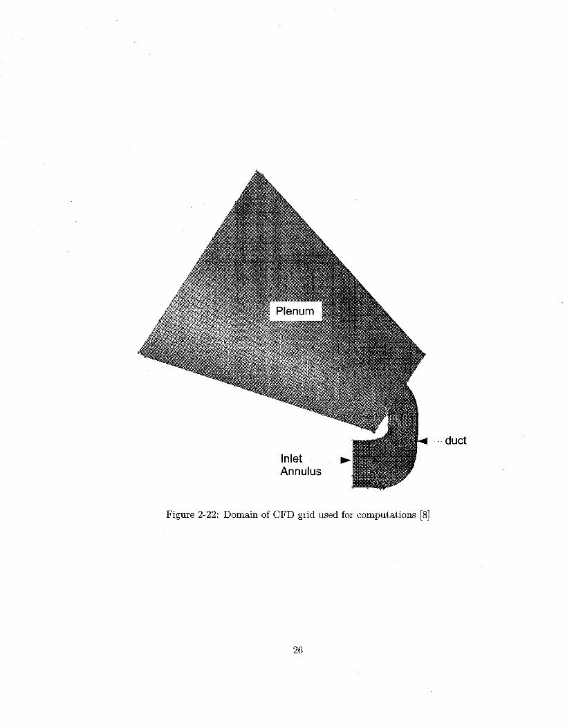
Computational Study
Five geometries were studied computationally. The computational domain consisted of an
inlet annulus, an exhaust duct, and a plenum chamber overlapping the exhaust duct exit,
Fig. 2-22. The plenum is a large conical domain with boundary conditions to allow the
exhaust jet to entrain flow freely into the plenum. The plenum also served to allow for
a non-uniform pressure distribution at the exhaust duct exit plane which results from the
large stream line curvature in the flow.
24
ffl n E ns
Figure 2-21: Schematic of experimental setup [8]
25
Plenum
7v \
*li\ . • • • • ' • . . . . ' . . . \
' • . . ' ; ; . . / . £'..••'„•-•' :'*.
• • ? * * . . " ' * ' • . * . - " . 4 . " *•
' * • . > ' * * J \
Inlet Annulus
• • - : : . . " • ' • • • i ^
••.•...-'•••-•• . " t r f c t i j
d u c t
Figure 2-22: Domain of CFD grid used for computations [8]
26
The computational grid was created using Gambit. Hexahedral elements were primarily
used to produce a structured mesh with only the annular to rectangular transitional region
requiring an unstructured grid composed of tetrahedral elements for ease of meshing. The
boundary layer was defined with prism elements in the first rows of mesh from the duct
surface. The flow solver used in this study was the commercial code Fluent 5.5. The most
suitable turbulence model which was available was the RNG k—e model; however the author
used the realizable k — e turbulence model through the majority of the study due to the
difficulty in obtaining a converged solution using the former.
Loss Mechanisms
Cunningham [8] has identified three geometric parameters affecting the total pressure losses
base on preliminary testing and literature:
1. Flow splitter.
2. Streamlining downstream of the center body.
3. Stub cross-sectional shape.
The three main pressure loss mechanisms were found and identified as:
1. Secondary flows: The secondary flows are generated through the duct bends as well
as the presence of the flow splitter redirecting the flow across the center-body.
2. Flow non-uniformity: Present at the stub exit representing undiffused kinetic energy
and therefore lower static pressure recovery. The exhaust stub cross-sectional shape
influenced the exit effective area-ratio.
3. Flow separation and recirculation: The total pressure losses are a function of the flow
separation and recirculation. Due to the complex shape of the exhaust duct, these
losses dominated over skin friction losses. Flow separation occurs along the inside
bend of the duct and in some cases, downstream of the center body.
27
Results and Conclusions
Cunningham [8] made a comparison of experimental and CFD results concluding that the
CFD consistently under-predicts the level of pressure losses in the exhaust ducts. CFD
has on the other hand shown that it is capable of capturing trends in losses by accurately
predicting changes in magnitude of pressure losses from one geometry to the next. When
comparing pressure losses due to inlet swirl, Cunningham found that the slope of the trend
line was under predicted when compared to measured results. This has been explained as
the inability of the turbulence models to handle the anisotropy of highly swirling flows.
Table 2.1 summarizes these findings.
Table 2.1: Summary of performance of CFD analysis in the study of single port gas turbine exhaust [8]
Parameter E
A P t t A Pts
geometry
flow structure
efficiency
inlet conditions
Suitability fair fair fair
good
fair
excellent
excellent
Comments Under-predicts distortion and secondary flow under-predicts losses under-predicts losses able to predict correct magnitude and trends with change in geometry easily gives details of internal flow structure, may not be reliable in identifying separation very efficient for studying inlet conditions, geometry limited by efficiency of mesher inlet conditions can be easily specified
If CFD is to be used to design optimum exhaust ducts, Cunningham has made the
following recommendations:
• In terms of predicting the total-to-static losses in the duct, the distribution of inlet
flow has a large effect on the distribution of the outlet flow. To be able to make a
realistic estimate of the total-to-static losses, a good estimate of the outlet flow is
required. To ensure this, velocity boundary conditions should be applied at the inlet
as this leads to a more realistic flow distribution at the exit.
28
• A large plenum is required at the exit of the duct to produce accurate flow distortions
in the duct near the exit.
• Turbulence models which account for swirl should be used if possible.
• Where possible, boundary conditions should be applied that account for the total
pressure non-uniformities at the duct inlet resulting from the presence of the engine.
29
Chapter 3
Design of Experiment
The work of Loka et al. [20], and Cunnigham [8] have identified many of the geometric and
aerodynamic parameters responsible for the overall duct loss. In this chapter, more param
eters are identified. Also discussed here are how the geometric parameters are quantified
and bounded within a specific design space, giving limits to the magnitude of each param
eter, for the purpose of creating a loss correlation. Next, combinations of each geometric
parameter are grouped together to create a set of exhaust duct models which, later, will be
simulated numerically along with the aerodynamic parameters to produce data for building
a loss correlation.
3.1 Geometric Design Space
A design space can be envisioned as being an n-dimensional box which is capable of contain
ing all practical exhaust duct shapes and sizes. The size of the box is chosen to allow each
geometric parameter to be varied from a minimum to a maximum value which is thought
to cover rather well the design space so that both good and bad performing exhaust ducts
are represented. For each parameter, a minimum of three changes are required to be able to
predict a non-linear trend with respect to exhaust duct losses. In this study, each geometric
parameter will be extended to the minimum and maximum limits of the design space with
one selection in the center.
30
3.1.1 Equivalent Cone Diffusion Angle
The exhaust duct region between the inlet and the flow splitter can be represented as an
annular duct. Quantifying an annulus using one parameter is done through an Equivalent
e f f iSS IS f f iBMSISSBSf f iSBBMWSlS lS lSEVV |& H K H S IS >S v IS S IS IS IS IS H IS IS IS IS S IS IS »3Q 6<iSSSSSiSiSiSSdiSKiSS>SiSiSSlSK?£^ e is is s s is ISIS <s s »is is si s is s s is vi
s is si s s >s is is sa s is si is si s Q g :i< m is x s is is is is s is is is & E S T
Figure 6-13: Mach number contour plot on a plane through the flow splitter
93
AR = 1.000 AS = 0.920
AR= 1.350 AS = 0.920
AR = 1.350 AS = 1.380
AR= 1.000 AS = 1.380
# <f & # & ^ ^ <? ^ & & # # ^ #
•H9H
Q inlet
Figure 6-14: Normalized wall static pressure contours demonstrating the effect of aspect ratio and area ratio in the annular to rectangular transition region
94
AR= 1.000 AS = 0.920
AR = 1.350 AS = 1.380
D AR= 1.350 AS = 0.920
l ) AR= 1.000 AS = 1.380
o < £ " # <0» *<"> N** N> <VS C?5 & <£ <& \* t £ A^ C\Q
ti5 ^ <y <s° v N* *o -^ v" -v* T> v "r v t? <b' <y o- cr <a* <v <y O* Q* O O- <y <S- <y O-
I L.
Mach Number
Figure 6-15: Mach number contours demonstrating the effect of aspect ratio and area ratio in the annular to rectangular transition region
95
in Fig. 6-15 support this theory demonstrating that small aspect ratios do lead to flow
separation off the inner surface of the exhaust duct reducing the available flow area in the
streamwise direction. It can be concluded that it is favorable to have the largest available
aspect ratio to maintain an attached flow.
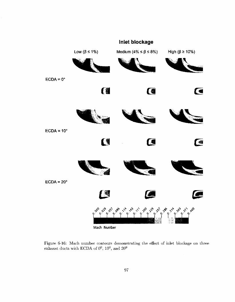
6.6 Effect of Inlet Boundary Layer Blockage
It has been found that the total pressure losses increase as a result of increasing inlet
boundary layer blockage. As seen in Fig. 6-16 a thick inlet boundary layer is more prone to
flow separation with the point of separation progressing closer to the inlet for thicker inlet
boundary layers. These results where expected when flowing against a positive pressure
gradient. The exhaust ducts with 20° ECDA demonstrated to have the most severe flow
separation over the other ECDA tested. The global effect of inlet blockage on all exhaust
ducts tested can be fully seen the Figs. 6-17 and 6-18. With low inlet blockage, there
no distinct relation to other tested geometric parameters, however increased blockage levels
have demonstrated higher levels of losses related to large inlet diffusion angles. It is apparent
in both figures that for medium and large inlet blockage, the exhaust ducts tested with 20°
ECDA have an overall higher trend of total pressure losses. When comparing medium to
high inlet blockage the same loss trends are found only at higher levels.
96
Inlet blockage
Low(3<1%)
I Medium (4% < B < 8%) High (8 2:10%)
ECDA = 0°
ECDA = 20°
en m (3
4l ECDA =10°
a ri Cm
C$ 1 ^ <?> 0$> «> t?> AN C? I 0 * «? o£> • > «?> V s C$ (? (i> ^ Q* V N5, <> f 'V' f f> V T V >°
c>- <v &• o- <a- o- Q- o- O' o- <y c>- cr o- <y J I ' ' '
Mach Number
Figure 6-16: Mach number contours demonstrating the effect of inlet blockage on three exhaust ducts with ECDA of 0°, 10°, and 20°
97
^
K vs. Inlet Swirl Low and Medium Inlet blockage (p)
0.400 :
0.350'
0.300'
0.260 • I
0.200 I
0.150 i I
0.100
1
0.050 •
0.000 :
• 1
1
0 > a
1 1
• •
0
5 t
a A
ECDA ECDA ECDA
= n° =10° =20°
B<1° o
D
• ! o
* • i D
A
4°<B<8° • 4 •
20 30 35 40
Inlet Swirl f)
jure 6-17: Total pressure loss coefficient vs. inlet swirl for low and medium inlet blockage
OH
I
3!
a,
J » 0.250
II
0.200 11
0.150
0.100
0.050
0.000
K vs. Inlet Swirl Medium and High Inlet blockage (p)
• I
• D
I
1
•! • " • " - " ' 1 ' ' | 1
•
• D
1 * o
ECDA ECDA ECDA
_
= 0° =10° =20°
,
£
zz
$m: 0
a D
• • D
i
£ A
B>10° • * •
Inlet Swirl (°)
jure 6-18: Total pressure loss coefficient vs. inlet swirl for medium and high inlet blockage
Chapter 7
Correlation of the Total to Total
Pressure Loss
A correlation is presented in the following sections where the total to total pressure loss
coefficient is related to the geometric and aerodynamic parameters based on the data pro
duced in the computational flow simulations. The resulting correlation serves as a suitable
tool for designers when involved in the preliminary design of annular to rectangular exhaust
ducts.
The results of the parametric study demonstrate that the geometry of the exhaust duct
produces a highly asymmetric flow field, under the influence of swirl, and flow separation is
almost unavoidable when the later is combined with inlet blockage. The favorable approach
to produce the loss correlation would be to build upon an exact solution of the Navier Stokes
equation which can be easily be interpreted by a designer. However, an exact solution to
the Navier Stokes equations does not exist for this complex geometry therefore a numerical
approach must be taken.
The development of a loss model can follow one of the following two approaches; 1)
a purely mathematical approach where a reduced order model or a surrogate model is
constructed from available data (eg. Artificial Neural Networks [25]), and 2) a physical
approach where a numerical correlation is composed of different terms each of which rep
resent the effect of one flow feature contributing to the loss. The first approach is a black
99
11 vs. AR only those points whose B1 is less than or equal to 0.06
• T1_
• I s If
#>
• '
•
t f •
eta = 0.72 + 3e*(-0.9 - 1.SAR)
1 1 1 1 0 1 2 3 4 5 6 7 8
AR
Figure 7-1: Diffuser effectiveness versus area ratio with low level inlet aerodynamic blockage and no inlet swirl [7]
box to the designer and does not provide the user with the same feedback as do physical
correlations produced by curve fitting. Through curve fitting, the correlation will provide
the user with a visual understanding of the functional relations which can even take on a
physical meaning of the data being analyzed. The approach taken in this work is the second
one, where the data is correlated through a curve fitting technique similar to what was used
by Japikse [7] where he correlated annular diffuser effectiveness using available published
data.
7.1 Japikse Correlation of Annular Diffusers
To start the process Japikse has first identified that area ratio is the dominant variable
related to diffuser effectiveness, once the data was screened for blockage, and noting that
inlet swirl has been to some extent taken care of through the definition of Cpi in equation
2.3. He then plotted the data versus area ratio, Fig. 7-1, and discovered that the data
followed an exponential trend.
With the equation found in Fig. 7-1, Japikse was able to move on to the other variables
100
r\ vs.«,
a. <
•
>
« 1 1
1
•
• b -
• • • • •
" ^ " — • - • J '
•
I I I
eta= 1.O5-O.M0W1.9
\t * <t
eta = 1.05-0. «)02«,*Z1
'•
i »
<>
25
«1
Figure 7-2: Diffuser effectiveness with principle geometric effects removed including data at all levels of inlet aerodynamic blockage [7]
by removing the effect of area ratio by dividing out the data by the new expression as
presented in Fig. 7-2. In this figure, the data has been plotted versus inlet swirl and has
revealed two trends. The upper trend represents diffusers experiencing mild stall while the
lower trend represents diffusers with substantial stall.
The data was again divided by the new equations defined in Fig. 7-2, and the with the
effects of area ratio and inlet swirl removed from the data Japikse then moved on to inlet
blockage as shown in Fig. 7-3. From this figure Japikse has determined that there are two
trends which have been defined. The lower trend (common blockage, "A"), which is seen
to passes through the square symbols, is data from Coladipietro et al. [18] where tests were
conducted at two different blockage levels. In these testes, inlet conditions consisted of a
clean uniform velocity profile where only the boundary layer thickness was varied. The upper
trend (classical profile blockage, "B") which shows that diffuser performance improves with
increasing inlet blockage comes from inlet conditions where the boundary layer becomes
fully developed and contains increase levels of turbulence and vorticity. Dividing the data
again by the new equations, Japikse represented the data versus inlet blockage in Fig. 7-3
101
il vs. Bi
Jt EC A or
ilJO
0.2
• ^ j
• ^ " • N I
ata- ' i . iK+ o.UB'in(b5l)
o
it
|y = 4.777364E+D1x i -1.217600E+01K +139214BE+Do|
r— „ B »
* " "A"
<>
o.oe
B1
Figure 7-3: Diffuser effectiveness with the principle effects of geometry and inlet swirl removed according to preceding correlations [7]
to reveal that the data has collapsed to a value of 1 ± .10.
The resulting set of equations produced by studying the data trends is the following:
Cp = CPi (ai , r 2 / r i , 62/61) V (AR) 77 ( « I ) r? (£1) (7.1)
Figure 7-4: Diffuser effectiveness with the principle effects of geometry, inlet swirl, and inlet blockage removed [7]
103
K vs. Inlet Swirl Low Inlet blockage (P < 1%)
C-l
=8 Co
• • v .
a, i 1
i
1
4
0.450-
0.400 -
0.350'
0.300
0.250 •
0.200;
0.150
0.100
0.050 •
0.000 :
0 5 10 15 20 25 30 35 40
Inlet Swirl (°)
Figure 7-5: Total pressure loss trend in the exhaust for low inlet blockage
7.2 Correlation of the CFD Results
It was demonstrated in Sec. 6.2 that the total pressure losses in the exhaust duct are
independent of the stub direction. For this reason it was chosen to correlate the exhaust
duct losses independently of the stub losses. The following section presents a corelation to
predict the total pressure losses between the inlet and section-12 as shown in Fig. 6-1. The
correlations produced in this work have been found with the help of Windows Excel and
the statistical package LAB Fit [26].
The fist parameter that demonstrated to have the first order impact on losses in the
exhaust duct is inlet swirl. When inlet blockage was varied some distinct trends appeared
which demonstrated different behaviors in the losses depending on the magnitude of diffusion
taking place in the annular inlet of the exhaust duct. For low inlet blockage (j3 ^ 1%) it
is possible to find a single trend which can be used to normalize the data, Fig. 7-5. For
medium inlet blockage (4% < (3 ^ 8%) one trend has been defined for an ECDA of 20° and
one for the lower values tested, Fig. 7-6. When high inlet blockage (/3 > 10%) is present a
104
0.450
0.400 •
r v j
t '6
•O ft, |
*5 3
**** ft.
3 •5 53,
0.350
0.300
0.250
0.200
* 0.150
0.100
0.050
0.D00
K vs. Inlet Swirl Medium Inlet blockage (4% < p < 3%)
Y »O.112800C«Sff (0.047726-Jf) ECDA 0'
10' 201
20 25 30 35 40
Inlet Swirl f)
Figure 7-6: Total pressure loss trend in the exhaust for medium inlet blockage
8 ft, I
ft,
•5
II
0.400 •
0.350
0.300
0.250
0.200
0.150
0.100
0.050
0.000
K vs. Inlet Swirl High Inlet blockage (p > 10%)
Y - 0.214385COS/{0.033095-A'Xl+#)
J = 0.1 limCOSH (0.047726-XXI+ #)
5=0.1
ECDA • 0° * 10° • 20°
Met Swirl (°)
Figure 7-7: Total pressure loss trend in the exhaust for large inlet blockage
105
Figure 7-8: Surface passing through normalized losses for ECDA and aspect ratio (Solid circles are points lying above the surface and hollow circles are points lying below)
correction factor is used to increase the level of the trends used to describe medium inlet
blockage, Fig. 7-7. To calculate the loss due to intermediate ECDA and blockage levels, it is
recommended to interpolate between the trends in Fig. 7-6 and then interpolated with Fig.
7-5 for smaller inlet blockage or select a smaller correction factor for higher inlet blockages.
The equations derived above have considered the contribution to the losses due to the
effect of swirl with some consideration to the annular inlet section defined by ECDA. After
normalizing the data with those equations the effect of swirl with some consideration to
ECDA have effectively been removed and the other contributing parameters can now be
evaluated.
The next parameter considered is the aspect ratio of the exhaust duct. A good fit to
the data could not be found after trials at correlating the aspect ratio to the normalized