80
Pricing Variable Quantities Sponsored by Defense Pricing and Contracting Mr. Stephen Rost Cost/Price Analyst, Air Force Life Cycle Management Center, Pricing Directorate October 6, 2021 1
Pricing Variable QuantitiesSponsored by Defense Pricing and Contracting
Mr. Stephen Rost
Cost/Price Analyst, Air Force Life Cycle Management Center, Pricing Directorate
October 6, 2021 1
Agenda / Index
• Introduction
• Band Pricing
• Reiterative Linear Pricing
• Pricing Curves
• Takeaways
2

Approaches to Pricing Variable Quantities
Introduction
3
Why Price Variable Quantities?
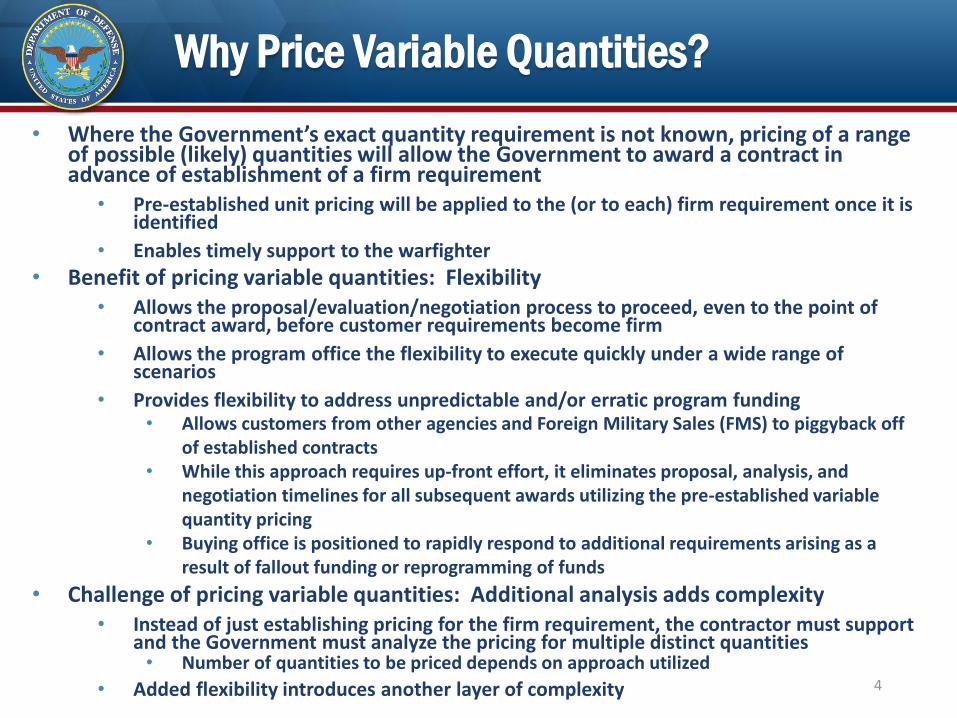
• Where the Government’s exact quantity requirement is not known, pricing of a range of possible (likely) quantities will allow the Government to award a contract in advance of establishment of a firm requirement
• Pre-established unit pricing will be applied to the (or to each) firm requirement once it is identified
• Enables timely support to the warfighter
• Benefit of pricing variable quantities: Flexibility• Allows the proposal/evaluation/negotiation process to proceed, even to the point of
contract award, before customer requirements become firm
• Allows the program office the flexibility to execute quickly under a wide range of scenarios
• Provides flexibility to address unpredictable and/or erratic program funding• Allows customers from other agencies and Foreign Military Sales (FMS) to piggyback off
of established contracts• While this approach requires up-front effort, it eliminates proposal, analysis, and
negotiation timelines for all subsequent awards utilizing the pre-established variable quantity pricing
• Buying office is positioned to rapidly respond to additional requirements arising as a result of fallout funding or reprogramming of funds
• Challenge of pricing variable quantities: Additional analysis adds complexity• Instead of just establishing pricing for the firm requirement, the contractor must support
and the Government must analyze the pricing for multiple distinct quantities • Number of quantities to be priced depends on approach utilized
• Added flexibility introduces another layer of complexity 4
Why Would Unit Pricing Vary as Quantity Changes?
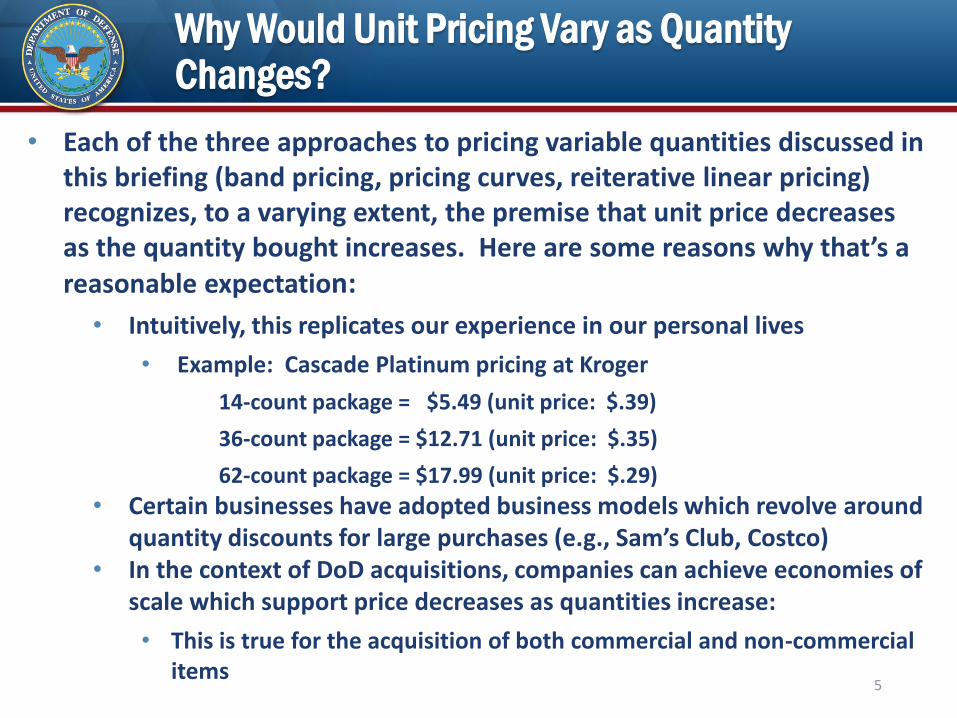
• Each of the three approaches to pricing variable quantities discussed in this briefing (band pricing, pricing curves, reiterative linear pricing) recognizes, to a varying extent, the premise that unit price decreases as the quantity bought increases. Here are some reasons why that’s a reasonable expectation:
• Intuitively, this replicates our experience in our personal lives
• Example: Cascade Platinum pricing at Kroger
14-count package = $5.49 (unit price: $.39)
36-count package = $12.71 (unit price: $.35)
62-count package = $17.99 (unit price: $.29)
• Certain businesses have adopted business models which revolve around quantity discounts for large purchases (e.g., Sam’s Club, Costco)
• In the context of DoD acquisitions, companies can achieve economies of scale which support price decreases as quantities increase:
• This is true for the acquisition of both commercial and non-commercial items
5
How Can Companies Achieve Economies of Scale?
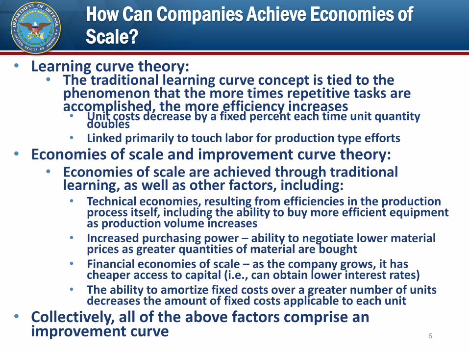
• Learning curve theory:• The traditional learning curve concept is tied to the
phenomenon that the more times repetitive tasks are accomplished, the more efficiency increases• Unit costs decrease by a fixed percent each time unit quantity
doubles• Linked primarily to touch labor for production type efforts
• Economies of scale and improvement curve theory:• Economies of scale are achieved through traditional
learning, as well as other factors, including:• Technical economies, resulting from efficiencies in the production
process itself, including the ability to buy more efficient equipment as production volume increases
• Increased purchasing power – ability to negotiate lower material prices as greater quantities of material are bought
• Financial economies of scale – as the company grows, it has cheaper access to capital (i.e., can obtain lower interest rates)
• The ability to amortize fixed costs over a greater number of units decreases the amount of fixed costs applicable to each unit
• Collectively, all of the above factors comprise an improvement curve 6
Definition of Fixed Costs
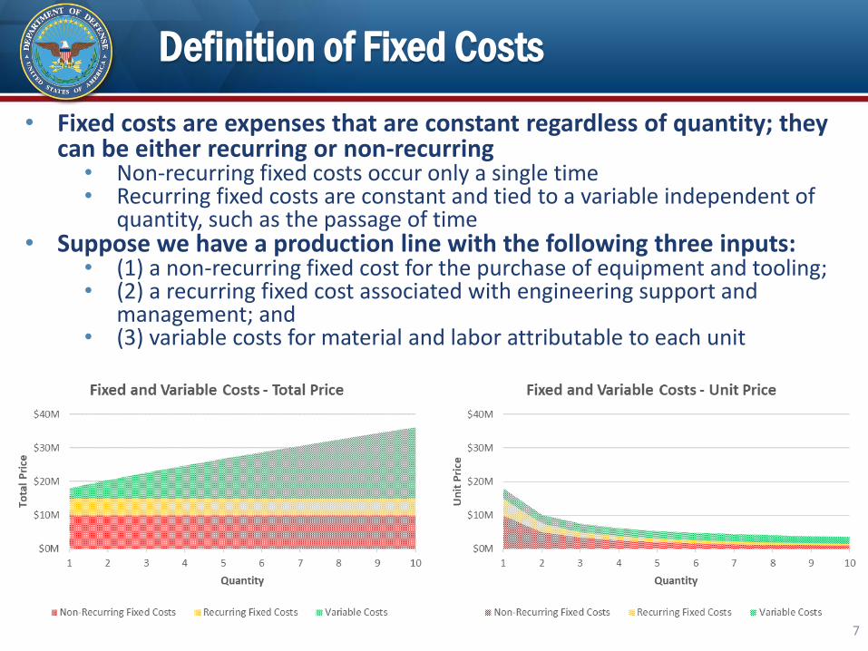
• Fixed costs are expenses that are constant regardless of quantity; they can be either recurring or non-recurring
• Non-recurring fixed costs occur only a single time• Recurring fixed costs are constant and tied to a variable independent of
quantity, such as the passage of time• Suppose we have a production line with the following three inputs:
• (1) a non-recurring fixed cost for the purchase of equipment and tooling;• (2) a recurring fixed cost associated with engineering support and
management; and• (3) variable costs for material and labor attributable to each unit
7
Amortization of Fixed Costs
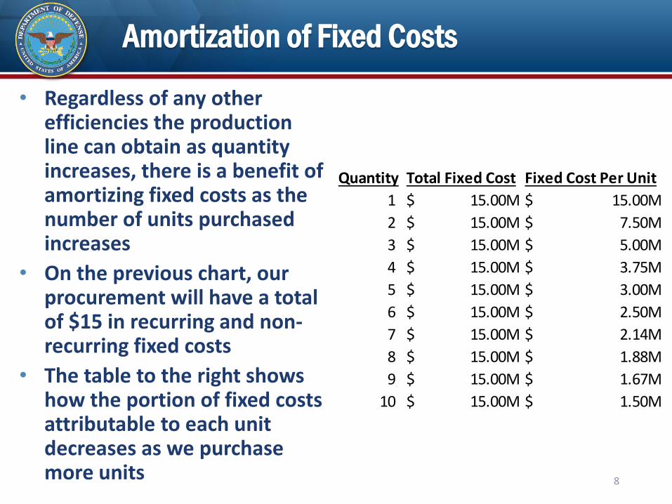
• Regardless of any other efficiencies the production line can obtain as quantity increases, there is a benefit of amortizing fixed costs as the number of units purchased increases
• On the previous chart, our procurement will have a total of $15 in recurring and non-recurring fixed costs
• The table to the right shows how the portion of fixed costs attributable to each unit decreases as we purchase more units 8
Quantity Total Fixed Cost Fixed Cost Per Unit
1 15.00M$ 15.00M$
2 15.00M$ 7.50M$
3 15.00M$ 5.00M$
4 15.00M$ 3.75M$
5 15.00M$ 3.00M$
6 15.00M$ 2.50M$
7 15.00M$ 2.14M$
8 15.00M$ 1.88M$
9 15.00M$ 1.67M$
10 15.00M$ 1.50M$
How to Price Fixed Costs
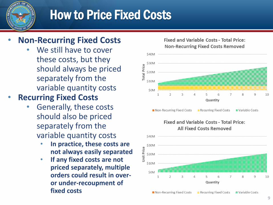
• Non-Recurring Fixed Costs• We still have to cover
these costs, but they should always be priced separately from the variable quantity costs
• Recurring Fixed Costs• Generally, these costs
should also be priced separately from the variable quantity costs• In practice, these costs are
not always easily separated• If any fixed costs are not
priced separately, multiple orders could result in over-or under-recoupment of fixed costs
9
How to Price Fixed Costs
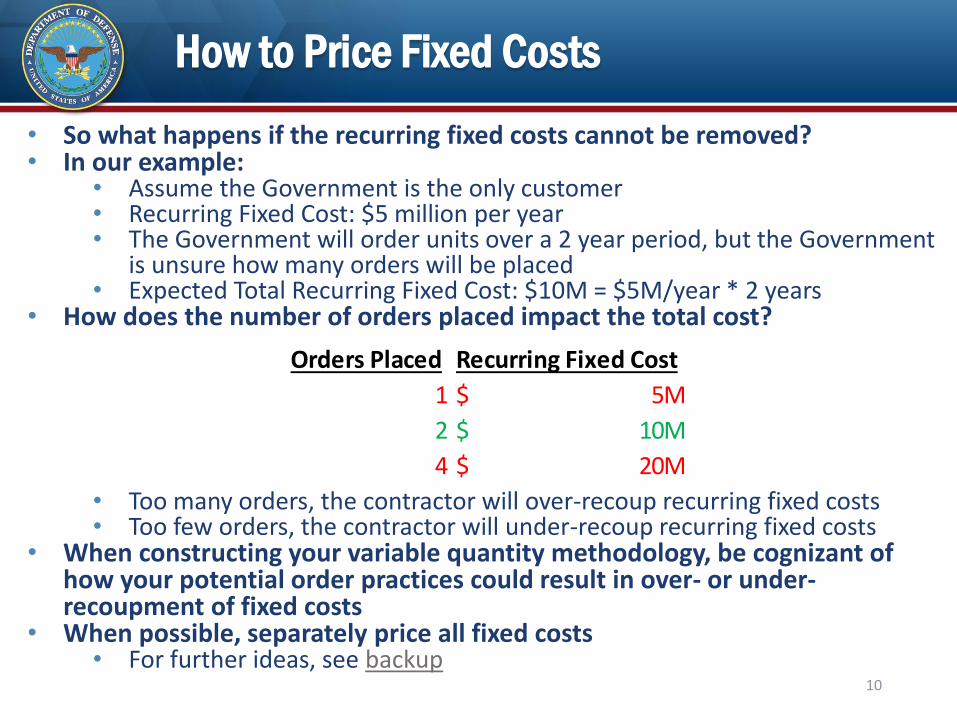
• So what happens if the recurring fixed costs cannot be removed?• In our example:
• Assume the Government is the only customer• Recurring Fixed Cost: $5 million per year• The Government will order units over a 2 year period, but the Government
is unsure how many orders will be placed• Expected Total Recurring Fixed Cost: $10M = $5M/year * 2 years
• How does the number of orders placed impact the total cost?
• Too many orders, the contractor will over-recoup recurring fixed costs• Too few orders, the contractor will under-recoup recurring fixed costs
• When constructing your variable quantity methodology, be cognizant of how your potential order practices could result in over- or under-recoupment of fixed costs
• When possible, separately price all fixed costs• For further ideas, see backup
10
Orders Placed Recurring Fixed Cost
1 5M$
2 10M$
4 20M$
Contract Instrument Application
• Under what contract instruments can we apply variable quantity methodologies?
• Indefinite delivery/indefinite quantity (IDIQ)• Used when
• a recurring need is anticipated;• the Government cannot predetermine, above a specified minimum,
the precise quantities of supplies or services that the Government will require during the contract period; and
• it is inadvisable for the Government to commit itself for more than a minimum quantity (FAR 16.504(b))
• When a pricing matrix (table or formula) for a range of quantities is established on the basic D contract, this allows orders to be placed for each requirement as it arises, using the pricing from the basic contract• Eliminates the need to separately price each requirement as it is
identified• Allows for efficient ordering
11
Contract Instrument Application
• “C” type contract with options
• Used when a single, firm requirement is anticipated for each option, but the option quantity is not known at time of negotiation of the basic requirement• A pricing matrix, with negotiated pricing for a range of possible
(likely) option quantities, is placed on contract
• At option exercise, the price from the matrix associated with the firm requirement quantity will be used to establish the exercised price of the option
• Allows the buying office to avoid “unpriced option” scenario Makes the option exercise administrative, reducing burden on both
contractor and buying office No need for new priced proposal for the option, with subsequent
evaluation and negotiation• This approach can provide an alternative to repetitive, standalone
annual procurements
12
Considerations for Selecting Contract Type
• Regardless of contract instrument, when selecting the contract type (pricing arrangement) remember the following:• All acquisitions have some degree of cost risk that must be
equitably allocated between the parties• Negotiating a variable quantity pricing matrix adds an additional
layer of cost risk that should be taken into consideration when selecting your contract type
• Variable Quantity Considerations:• How accurate is the selected variable quantity pricing
methodology?• How does the selected contract type support the parties’
equitable sharing of the cost risk associated with pricing a variation in quantity?
• For non-commercial contracts, you may wish to consider use of an incentive type contract to facilitate the sharing of cost risk inherent to variable quantity pricing arrangements
13
Order Aggregation
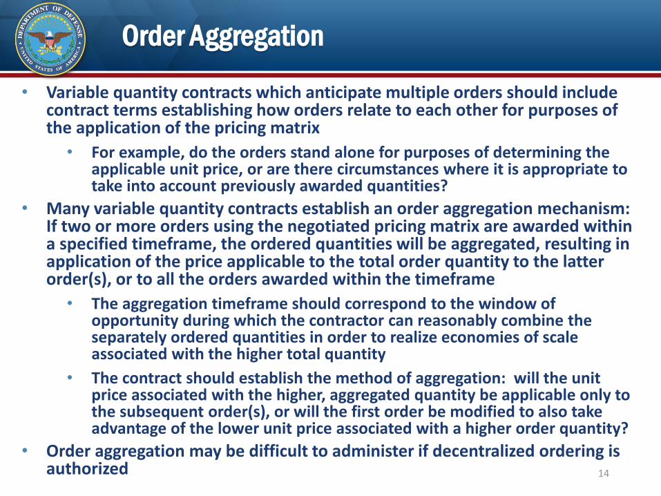
• Variable quantity contracts which anticipate multiple orders should include contract terms establishing how orders relate to each other for purposes of the application of the pricing matrix
• For example, do the orders stand alone for purposes of determining the applicable unit price, or are there circumstances where it is appropriate to take into account previously awarded quantities?
• Many variable quantity contracts establish an order aggregation mechanism: If two or more orders using the negotiated pricing matrix are awarded within a specified timeframe, the ordered quantities will be aggregated, resulting in application of the price applicable to the total order quantity to the latter order(s), or to all the orders awarded within the timeframe
• The aggregation timeframe should correspond to the window of opportunity during which the contractor can reasonably combine the separately ordered quantities in order to realize economies of scale associated with the higher total quantity
• The contract should establish the method of aggregation: will the unit price associated with the higher, aggregated quantity be applicable only to the subsequent order(s), or will the first order be modified to also take advantage of the lower unit price associated with a higher order quantity?
• Order aggregation may be difficult to administer if decentralized ordering is authorized 14
Order Aggregation Example
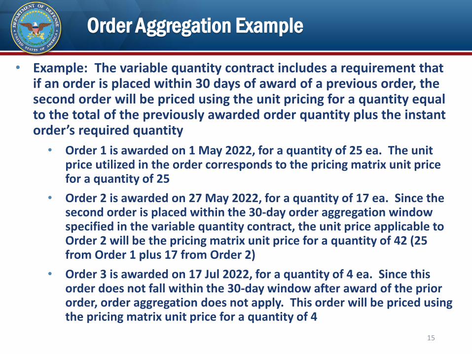
• Example: The variable quantity contract includes a requirement that if an order is placed within 30 days of award of a previous order, the second order will be priced using the unit pricing for a quantity equal to the total of the previously awarded order quantity plus the instant order’s required quantity
• Order 1 is awarded on 1 May 2022, for a quantity of 25 ea. The unit price utilized in the order corresponds to the pricing matrix unit price for a quantity of 25
• Order 2 is awarded on 27 May 2022, for a quantity of 17 ea. Since the second order is placed within the 30-day order aggregation window specified in the variable quantity contract, the unit price applicable to Order 2 will be the pricing matrix unit price for a quantity of 42 (25 from Order 1 plus 17 from Order 2)
• Order 3 is awarded on 17 Jul 2022, for a quantity of 4 ea. Since this order does not fall within the 30-day window after award of the prior order, order aggregation does not apply. This order will be priced using the pricing matrix unit price for a quantity of 4
15
Bend Your Thinking!
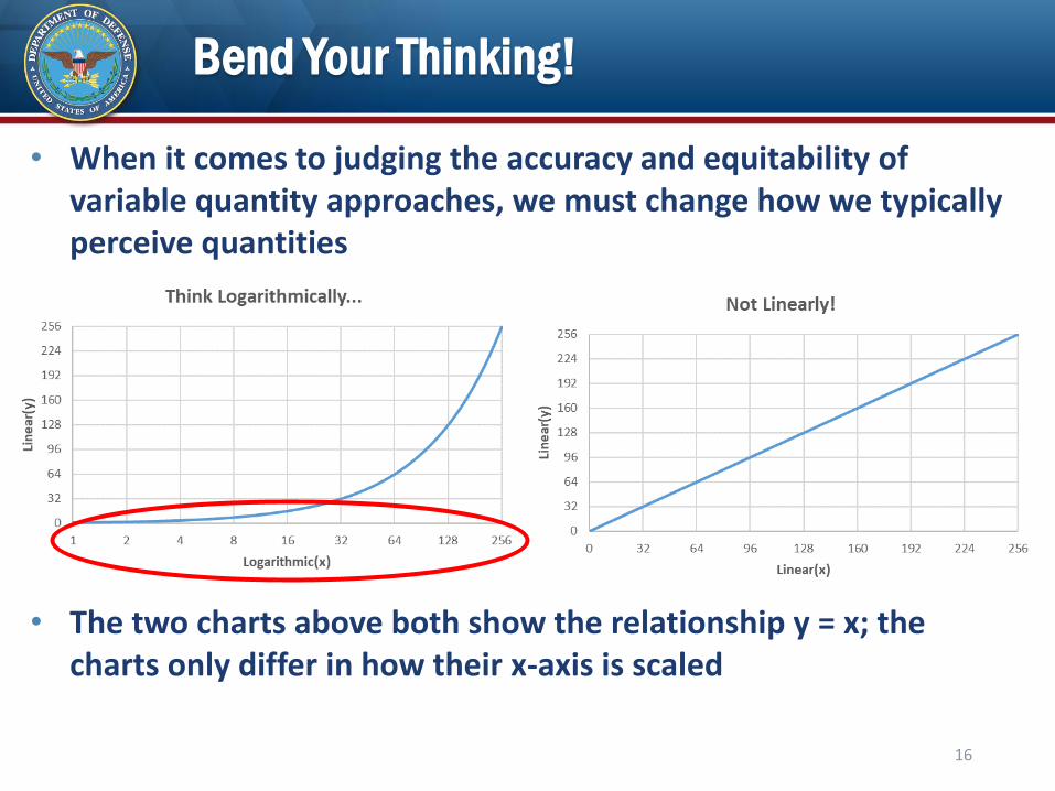
• When it comes to judging the accuracy and equitability of variable quantity approaches, we must change how we typically perceive quantities
• The two charts above both show the relationship y = x; the charts only differ in how their x-axis is scaled
16
Bend Your Thinking!
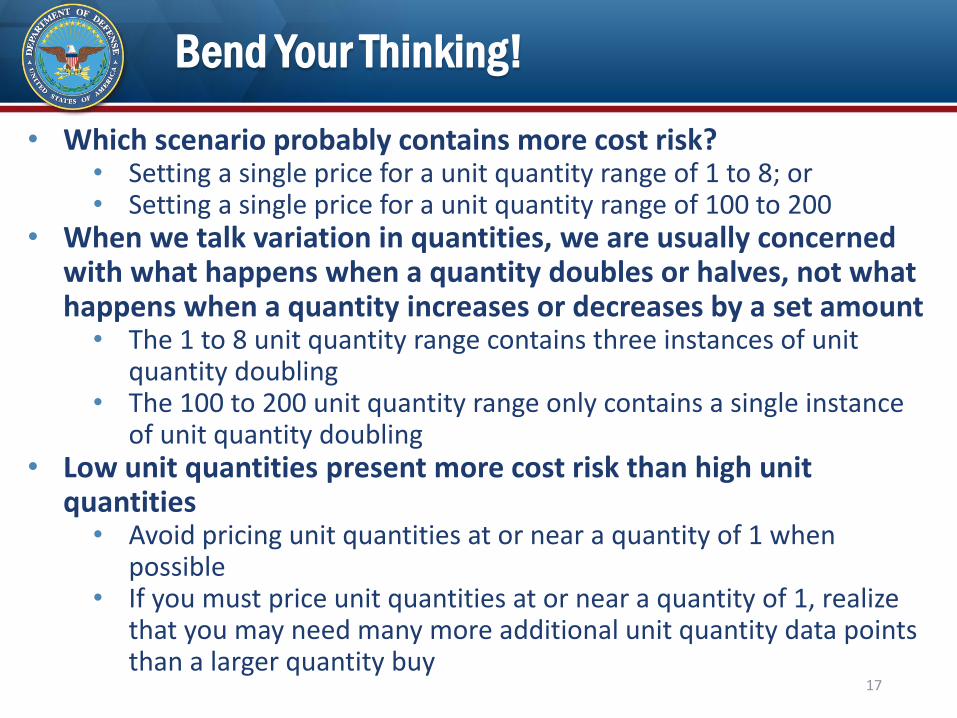
• Which scenario probably contains more cost risk?• Setting a single price for a unit quantity range of 1 to 8; or• Setting a single price for a unit quantity range of 100 to 200
• When we talk variation in quantities, we are usually concerned with what happens when a quantity doubles or halves, not what happens when a quantity increases or decreases by a set amount• The 1 to 8 unit quantity range contains three instances of unit
quantity doubling• The 100 to 200 unit quantity range only contains a single instance
of unit quantity doubling• Low unit quantities present more cost risk than high unit
quantities• Avoid pricing unit quantities at or near a quantity of 1 when
possible• If you must price unit quantities at or near a quantity of 1, realize
that you may need many more additional unit quantity data points than a larger quantity buy
17
Approaches to Pricing Variable Quantities
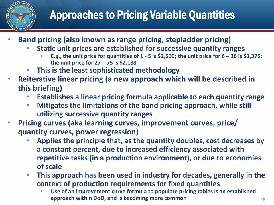
• Band pricing (also known as range pricing, stepladder pricing)• Static unit prices are established for successive quantity ranges
• E.g., the unit price for quantities of 1 - 5 is $2,500; the unit price for 6 – 26 is $2,375; the unit price for 27 – 75 is $2,188
• This is the least sophisticated methodology• Reiterative linear pricing (a new approach which will be described in
this briefing)• Establishes a linear pricing formula applicable to each quantity range• Mitigates the limitations of the band pricing approach, while still
utilizing successive quantity ranges• Pricing curves (aka learning curves, improvement curves, price/
quantity curves, power regression)• Applies the principle that, as the quantity doubles, cost decreases by
a constant percent, due to increased efficiency associated with repetitive tasks (in a production environment), or due to economies of scale
• This approach has been used in industry for decades, generally in the context of production requirements for fixed quantities• Use of an improvement curve formula to populate pricing tables is an established
approach within DoD, and is becoming more common 18
Approaches to Pricing Variable Quantities: Common Example
• To demonstrate and assess the relative merits of potential variable quantity pricing approaches, we will use a common example across all of the subsequent charts
• In the common example, the Government is procuring new radomes in support of retrofitting attack aircraft
• The Government wants flexibility to order anywhere between 4 to 64 units each quarter for the next calendar year. The quantity of radomes ordered in a given quarter will be subject to fluctuation depending upon the availability of funding and aircraft depot throughput
• In order to support efficient ordering and minimize the administrative and analytical burden of proposal preparation, proposal evaluation, and negotiations, the parties have agreed to negotiate a variable quantity pricing matrix
• The Government’s acquisition strategy for this example must take into account Contractor costs associated with acquiring the necessary subcomponent material, non-recurring costs to set up the production line tooling, and recurring production costs such as production labor, quality control, engineering support, and management• Remember: best practice is to segregate fixed costs and establish approaches for recognizing these costs
at the rate they are incurred (a single time; once per order, regardless of order quantity; once per year, etc.)
• If fixed costs cannot be segregated, be aware of how your potential order practices could result in over-or under-recoupment of fixed costs
19
Approaches to Pricing Variable Quantities: Common Example
• In the common example, the parties have already accomplished the following:
• The Contractor has proposed pricing and provided supporting data for select data points (quantities) specified in the RFP
• The Government has conducted fact-finding, a technical evaluation, and the necessary analysis pursuant to FAR Part 15
• Through the process of negotiations, the parties reached a fair and reasonable settlement on the price for each of the quantities analyzed
• The hard work is done! Now the parties must use the data points represented by the priced quantities to establish pricing for all the other quantities between 4 and 64 for which prices have not yet been negotiated. This presentation will focus on three potential approaches:
• Band Pricing• Reiterative Linear Pricing• Pricing Curves
• This presentation will then measure the results of each variable quantity pricing approach against a what-if alternate reality where both parties had sufficient resources to propose, evaluate, and negotiate fair and reasonable unit prices for every unit quantity from 4 to 64
20
Approaches to Pricing Variable Quantities: Graphic View
21
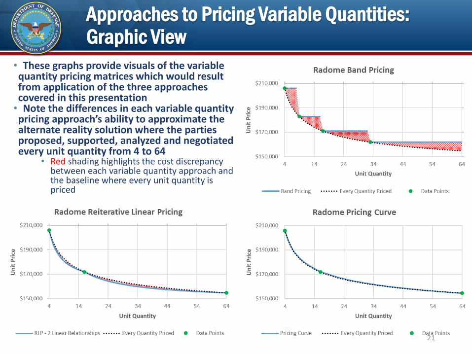
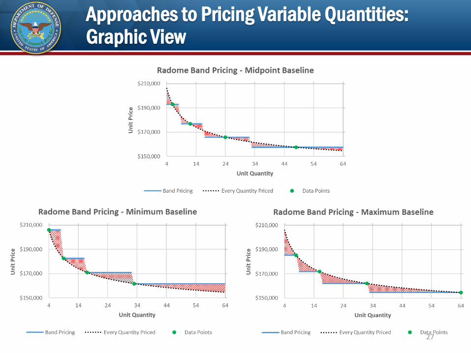
• These graphs provide visuals of the variable quantity pricing matrices which would result from application of the three approaches covered in this presentation• Note the differences in each variable quantity pricing approach’s ability to approximate the alternate reality solution where the parties proposed, supported, analyzed and negotiated every unit quantity from 4 to 64
• Red shading highlights the cost discrepancy between each variable quantity approach and the baseline where every unit quantity is priced
Approaches to Pricing Variable Quantities
Band Pricing
22
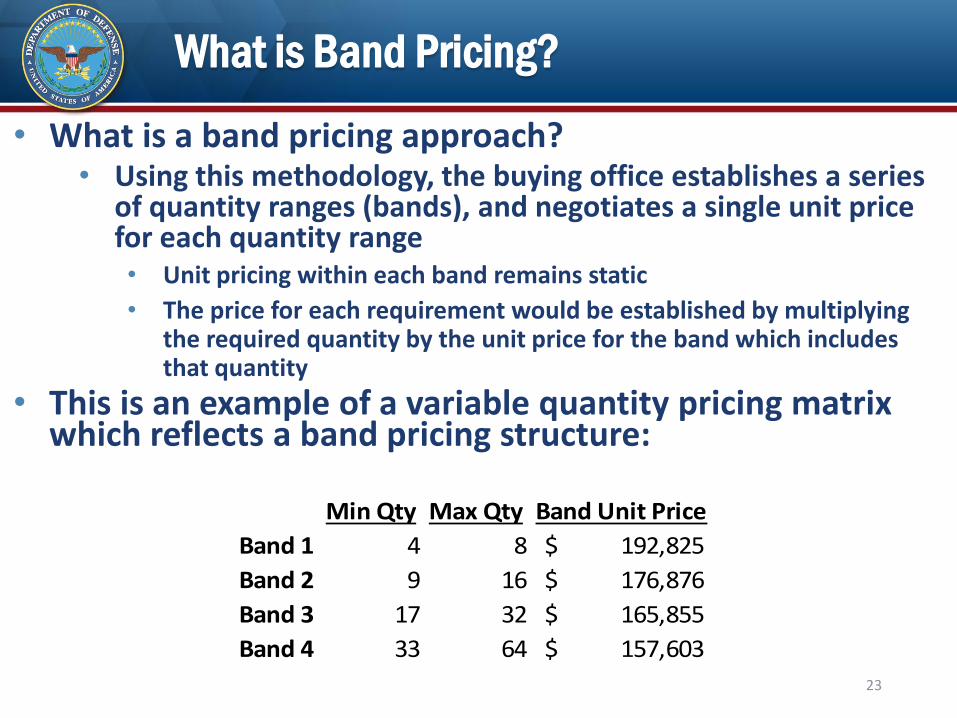
What is Band Pricing?
• What is a band pricing approach?• Using this methodology, the buying office establishes a series
of quantity ranges (bands), and negotiates a single unit price for each quantity range• Unit pricing within each band remains static
• The price for each requirement would be established by multiplying the required quantity by the unit price for the band which includes that quantity
• This is an example of a variable quantity pricing matrix which reflects a band pricing structure:
23
Min Qty Max Qty Band Unit Price
Band 1 4 8 192,825$
Band 2 9 16 176,876$
Band 3 17 32 165,855$
Band 4 33 64 157,603$
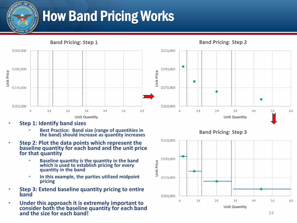
How Band Pricing Works
• Step 1: Identify band sizes• Best Practice: Band size (range of quantities in
the band) should increase as quantity increases
• Step 2: Plot the data points which represent the baseline quantity for each band and the unit price for that quantity
• Baseline quantity is the quantity in the band which is used to establish pricing for every quantity in the band
• In this example, the parties utilized midpoint pricing
• Step 3: Extend baseline quantity pricing to entire band
• Under this approach it is extremely important to consider both the baseline quantity for each band and the size for each band! 24
Band Pricing Considerations: Which Baseline Quantity is Used to Establish Range Unit Price?
• Under the band pricing approach, a single quantity within each band – the baseline quantity – is used to establish the unit price for the entire range of quantities in each band • The parties propose/ evaluate/ negotiate the price of each
band’s baseline quantity to establish the unit pricing applicable to every quantity included in each band
• BUT, how do the parties establish the baseline quantities?
• Some possible positions as to which unit to price as the baseline quantity for each band include:
• The minimum band quantity
• The maximum band quantity
• The midpoint band quantity
• Which approach do you think is most equitable to both parties? Why? 25
Band Pricing Considerations: Which Baseline Quantity is Used to Establish Range Unit Price?
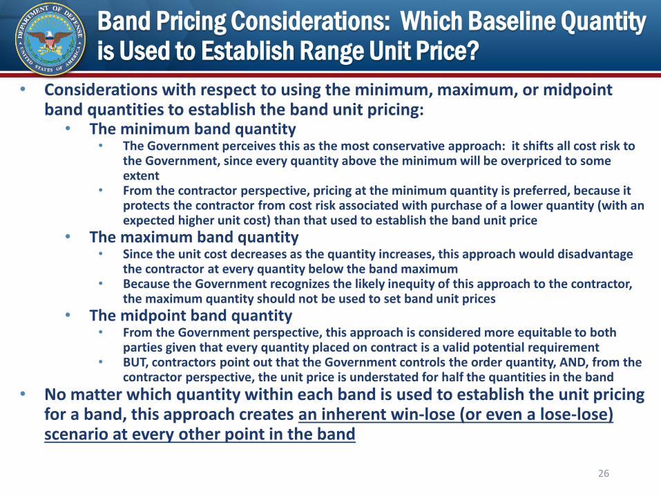
• Considerations with respect to using the minimum, maximum, or midpoint band quantities to establish the band unit pricing:
• The minimum band quantity• The Government perceives this as the most conservative approach: it shifts all cost risk to
the Government, since every quantity above the minimum will be overpriced to some extent
• From the contractor perspective, pricing at the minimum quantity is preferred, because it protects the contractor from cost risk associated with purchase of a lower quantity (with an expected higher unit cost) than that used to establish the band unit price
• The maximum band quantity• Since the unit cost decreases as the quantity increases, this approach would disadvantage
the contractor at every quantity below the band maximum• Because the Government recognizes the likely inequity of this approach to the contractor,
the maximum quantity should not be used to set band unit prices
• The midpoint band quantity• From the Government perspective, this approach is considered more equitable to both
parties given that every quantity placed on contract is a valid potential requirement • BUT, contractors point out that the Government controls the order quantity, AND, from the
contractor perspective, the unit price is understated for half the quantities in the band
• No matter which quantity within each band is used to establish the unit pricing for a band, this approach creates an inherent win-lose (or even a lose-lose) scenario at every other point in the band
26
Approaches to Pricing Variable Quantities: Graphic View
27

Variable Quantities Priced at Minimum Band Quantity
Assume, for our example, the Government considers that it negotiated a 12% profit rate. As the quantity increases from the min of the band to the max, the negotiated price is increasingly overstated, to the extent that appropriate economies of scale, including amortization of fixed costs over higher quantities, are not captured in the band price based on the minimum quantity. This creates the potential for large unintended profit amounts (unrelated to the company’s ability to control cost) and effectively makes the negotiated profit rate of 12% a minimum profit.
WIN-LOSE SCENARIO
All of the cost risk associated with the variable quantity has been shifted to the
Government
Average potential profit over all points is 16%
Potential profit as high as 20% 28
Variable Quantities Priced at Maximum Band Quantity
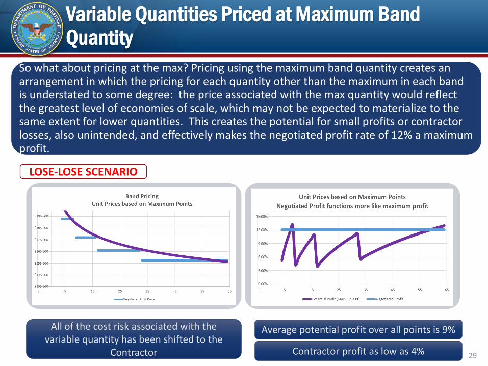
So what about pricing at the max? Pricing using the maximum band quantity creates an arrangement in which the pricing for each quantity other than the maximum in each band is understated to some degree: the price associated with the max quantity would reflect the greatest level of economies of scale, which may not be expected to materialize to the same extent for lower quantities. This creates the potential for small profits or contractor losses, also unintended, and effectively makes the negotiated profit rate of 12% a maximum profit.
LOSE-LOSE SCENARIO
All of the cost risk associated with the variable quantity has been shifted to the
Contractor
Average potential profit over all points is 9%
Contractor profit as low as 4% 29
Variable Quantities Priced at Midpoint Band Quantity
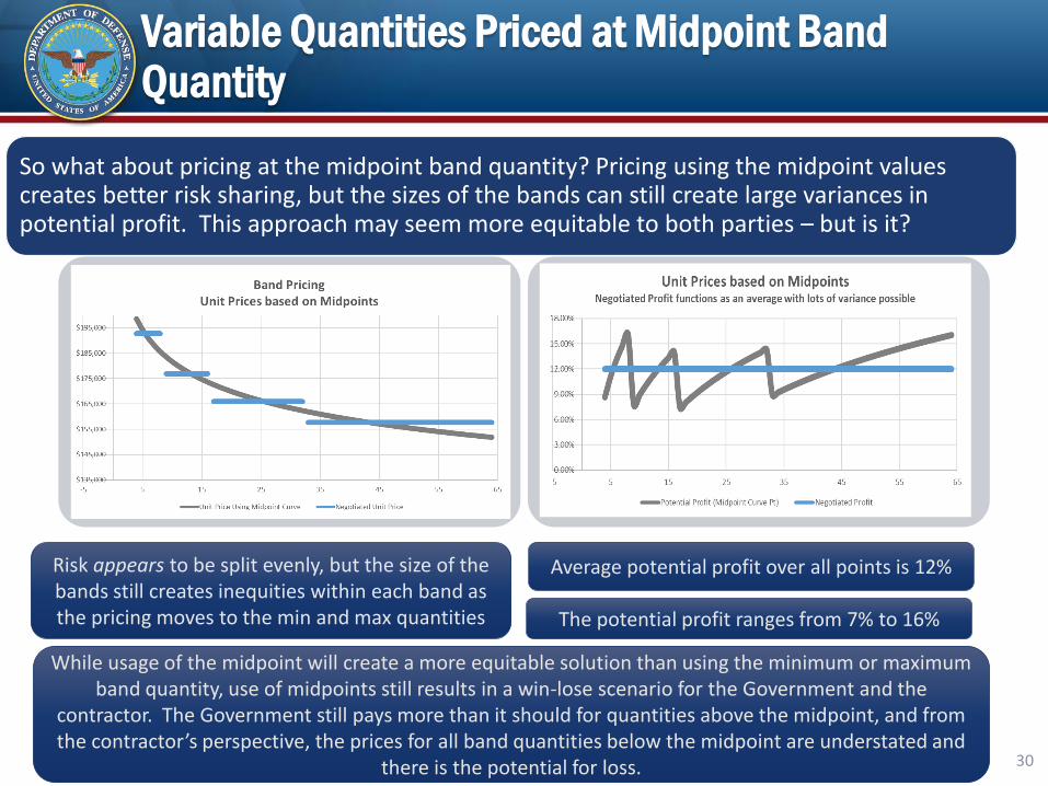
So what about pricing at the midpoint band quantity? Pricing using the midpoint values creates better risk sharing, but the sizes of the bands can still create large variances in potential profit. This approach may seem more equitable to both parties – but is it?
Risk appears to be split evenly, but the size of the bands still creates inequities within each band as the pricing moves to the min and max quantities
Average potential profit over all points is 12%
The potential profit ranges from 7% to 16%
While usage of the midpoint will create a more equitable solution than using the minimum or maximum band quantity, use of midpoints still results in a win-lose scenario for the Government and the
contractor. The Government still pays more than it should for quantities above the midpoint, and from the contractor’s perspective, the prices for all band quantities below the midpoint are understated and
there is the potential for loss. 30
Variable Quantities Priced at Min, Mid, Max
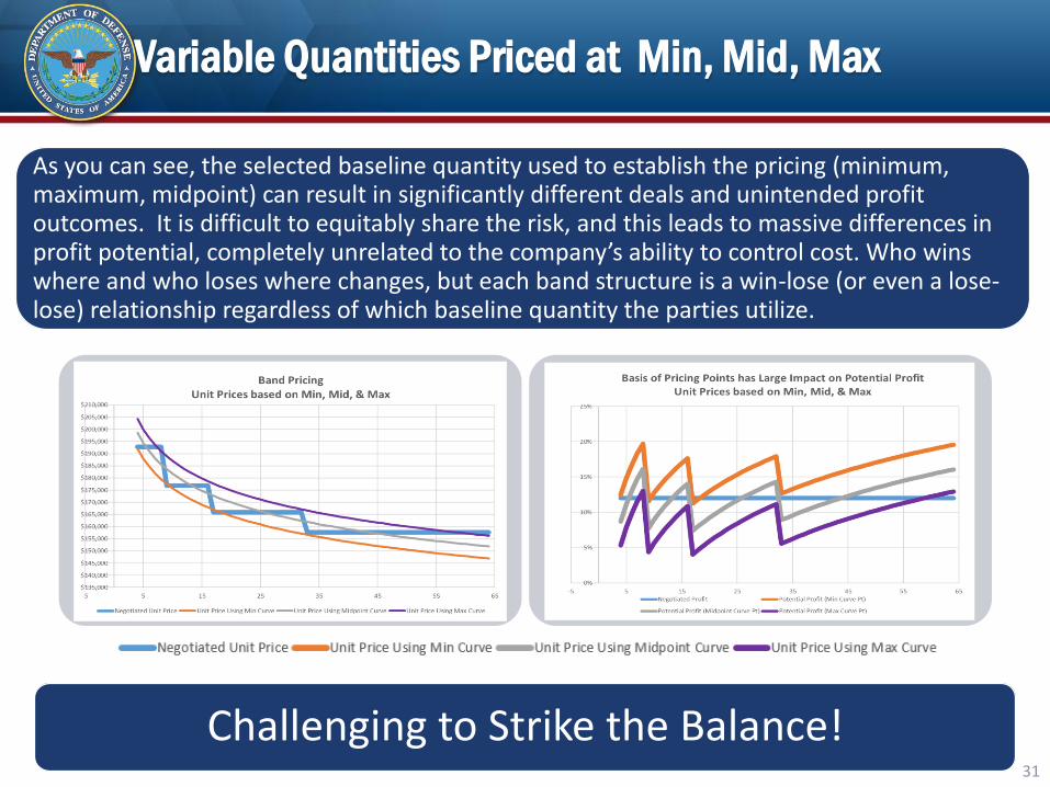
As you can see, the selected baseline quantity used to establish the pricing (minimum, maximum, midpoint) can result in significantly different deals and unintended profit outcomes. It is difficult to equitably share the risk, and this leads to massive differences in profit potential, completely unrelated to the company’s ability to control cost. Who wins where and who loses where changes, but each band structure is a win-lose (or even a lose-lose) relationship regardless of which baseline quantity the parties utilize.
Challenging to Strike the Balance!31
Band Pricing Considerations: Sizes of the Bands
• Sizes of the bands: When using band pricing, the buying office should identify the min and max of each band to be priced• Important to be thoughtful when establishing band sizes• Remember the price/quantity curve theory mentioned earlier?
“As the quantity doubles, the cost decreases by a constant percent.” • Although the band pricing approach generally doesn’t take
price/quantity curve theory into account, it still applies • For this reason, teams should be cognizant of the sizes of the bands
• Assuming an improvement curve of 90%, there is 10% savings every time the quantity doubles
• If a band is extremely wide, e.g. 200 – 800 units, note that the quantity doubles twice between the band minimum and maximum, while the unit price for the band remains constant
• If pricing is established based on the minimum quantity, the Government would be forgoing 10% savings at a quantity of 400 and 20% savings at the maximum quantity
• Even if the parties established the band price at a quantity of 400, the Government would forego 10% savings at the maximum quantity, and the Contractor would experience a 10% loss at the minimum quantity
• In order to account for the cost risk associated with this variable quantity methodology, the Government should avoid instances of multiple unit quantity doubling within a single band• Consider whether the size of bands should increase as quantity
increases 32
Band Pricing Considerations: Sizes of the Bands
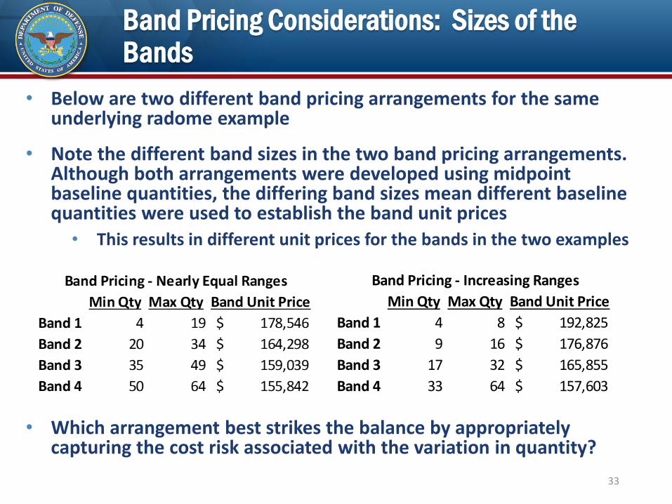
• Below are two different band pricing arrangements for the same underlying radome example
• Note the different band sizes in the two band pricing arrangements. Although both arrangements were developed using midpoint baseline quantities, the differing band sizes mean different baseline quantities were used to establish the band unit prices
• This results in different unit prices for the bands in the two examples
• Which arrangement best strikes the balance by appropriately capturing the cost risk associated with the variation in quantity?
33
Min Qty Max Qty Band Unit Price
Band 1 4 8 192,825$
Band 2 9 16 176,876$
Band 3 17 32 165,855$
Band 4 33 64 157,603$
Band Pricing - Increasing Ranges
Band Pricing Considerations: Sizes of the Bands
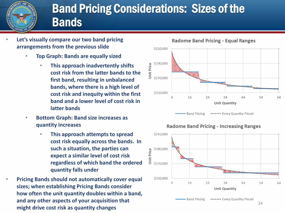
• Let’s visually compare our two band pricing arrangements from the previous slide
• Top Graph: Bands are equally sized
• This approach inadvertently shifts cost risk from the latter bands to the first band, resulting in unbalanced bands, where there is a high level of cost risk and inequity within the first band and a lower level of cost risk in latter bands
• Bottom Graph: Band size increases as quantity increases
• This approach attempts to spread cost risk equally across the bands. In such a situation, the parties can expect a similar level of cost risk regardless of which band the ordered quantity falls under
• Pricing Bands should not automatically cover equal sizes; when establishing Pricing Bands consider how often the unit quantity doubles within a band, and any other aspects of your acquisition that might drive cost risk as quantity changes
34
Band Pricing Considerations: Sizes of the Bands
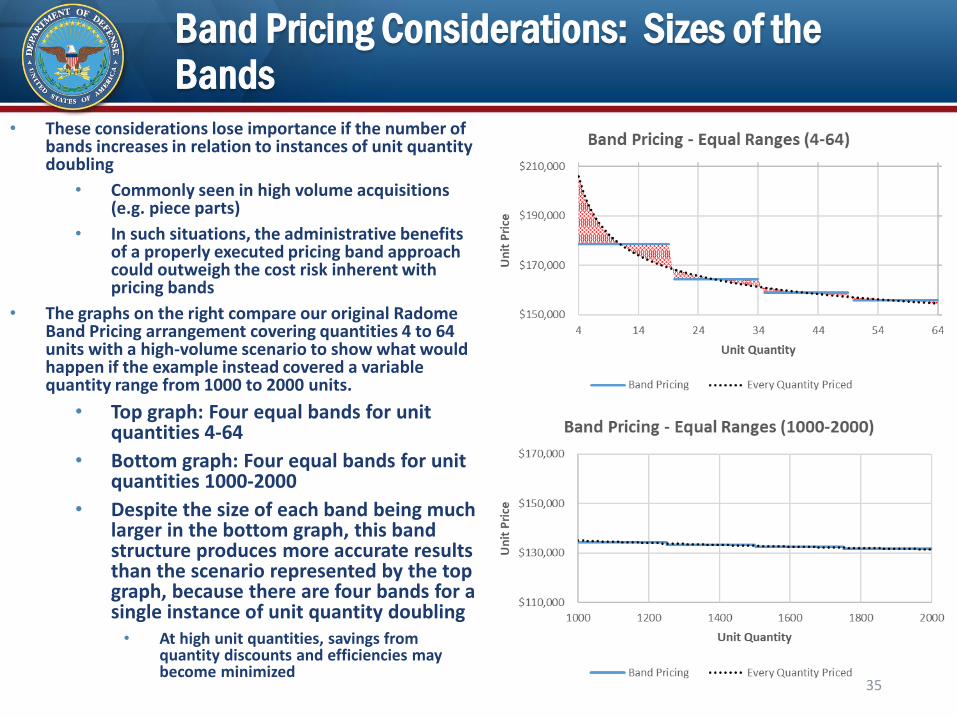
• These considerations lose importance if the number of bands increases in relation to instances of unit quantity doubling
• Commonly seen in high volume acquisitions (e.g. piece parts)
• In such situations, the administrative benefits of a properly executed pricing band approach could outweigh the cost risk inherent with pricing bands
• The graphs on the right compare our original Radome Band Pricing arrangement covering quantities 4 to 64 units with a high-volume scenario to show what would happen if the example instead covered a variable quantity range from 1000 to 2000 units.
• Top graph: Four equal bands for unit quantities 4-64
• Bottom graph: Four equal bands for unit quantities 1000-2000
• Despite the size of each band being much larger in the bottom graph, this band structure produces more accurate results than the scenario represented by the top graph, because there are four bands for a single instance of unit quantity doubling• At high unit quantities, savings from
quantity discounts and efficiencies may become minimized
35
Band Pricing: How Many Data Points?
36
• Under the Band Pricing approach, the Government must thoughtfully establish the number and size of bands to be priced, to reduce risk to both parties• This drives the number of data points (band baseline
quantities) that must be proposed, evaluated, and negotiated• Bands that are too big are problematic
• If the quantity doubles within a band, the parties are foregoing some measure of price decrease/increase based on the applicable improvement curve
• Increasing predictive accuracy through creating smaller bands in turn leads to a larger number of bands• This means the parties must propose, evaluate, and negotiate a
higher number of data points -> increased complexity
• Recommended rule of thumb for small quantity acquisitions: request a data point (at least) every time the quantity doubles
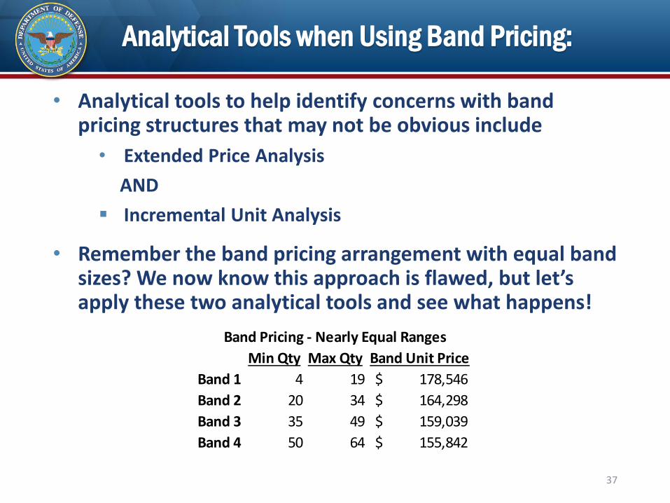
Analytical Tools when Using Band Pricing:
• Analytical tools to help identify concerns with band pricing structures that may not be obvious include
• Extended Price Analysis
AND
Incremental Unit Analysis
• Remember the band pricing arrangement with equal band sizes? We now know this approach is flawed, but let’s apply these two analytical tools and see what happens!
37
Min Qty Max Qty Band Unit Price
Band 1 4 19 178,546$
Band 2 20 34 164,298$
Band 3 35 49 159,039$
Band 4 50 64 155,842$
Band Pricing - Nearly Equal Ranges
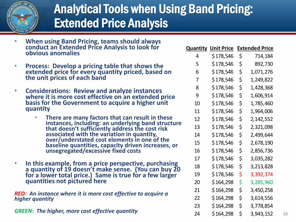
Analytical Tools when Using Band Pricing: Extended Price Analysis
• When using Band Pricing, teams should always conduct an Extended Price Analysis to look for obvious anomalies
• Process: Develop a pricing table that shows the extended price for every quantity priced, based on the unit prices of each band
• Considerations: Review and analyze instances where it is more cost effective on an extended price basis for the Government to acquire a higher unit quantity
• There are many factors that can result in these instances, including: an underlying band structure that doesn’t sufficiently address the cost risk associated with the variation in quantity, over/understated cost elements in one of the baseline quantities, capacity driven increases, or unsegregated/excessive fixed costs
• In this example, from a price perspective, purchasing a quantity of 19 doesn’t make sense. (You can buy 20 for a lower total price.) Same is true for a few larger quantities not pictured here
RED: An instance where it is more cost effective to acquire a higher quantity
GREEN: The higher, more cost effective quantity38
Quantity Unit Price Extended Price
4 178,546$ 714,184$
5 178,546$ 892,730$
6 178,546$ 1,071,276$
7 178,546$ 1,249,822$
8 178,546$ 1,428,368$
9 178,546$ 1,606,914$
10 178,546$ 1,785,460$
11 178,546$ 1,964,006$
12 178,546$ 2,142,552$
13 178,546$ 2,321,098$
14 178,546$ 2,499,644$
15 178,546$ 2,678,190$
16 178,546$ 2,856,736$
17 178,546$ 3,035,282$
18 178,546$ 3,213,828$
19 178,546$ 3,392,374$
20 164,298$ 3,285,960$
21 164,298$ 3,450,258$
22 164,298$ 3,614,556$
23 164,298$ 3,778,854$
24 164,298$ 3,943,152$
Analytical Tools when Using Band Pricing: Incremental Unit Analysis
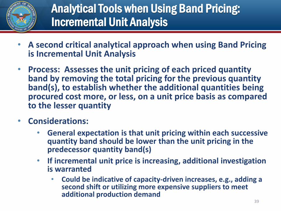
• A second critical analytical approach when using Band Pricing is Incremental Unit Analysis
• Process: Assesses the unit pricing of each priced quantity band by removing the total pricing for the previous quantity band(s), to establish whether the additional quantities being procured cost more, or less, on a unit price basis as compared to the lesser quantity
• Considerations:• General expectation is that unit pricing within each successive
quantity band should be lower than the unit pricing in the predecessor quantity band(s)
• If incremental unit price is increasing, additional investigation is warranted • Could be indicative of capacity-driven increases, e.g., adding a
second shift or utilizing more expensive suppliers to meet additional production demand
39
Analytical Tools when Using Band Pricing: Incremental Unit Analysis
40
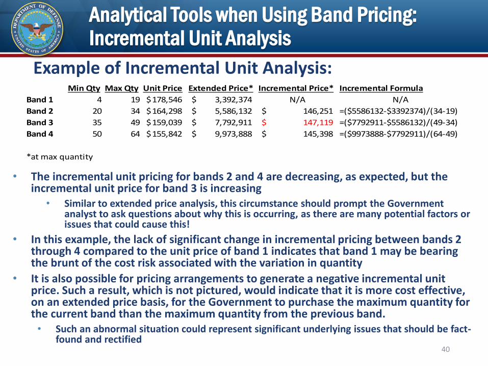
Example of Incremental Unit Analysis:
• The incremental unit pricing for bands 2 and 4 are decreasing, as expected, but the incremental unit price for band 3 is increasing
• Similar to extended price analysis, this circumstance should prompt the Government analyst to ask questions about why this is occurring, as there are many potential factors or issues that could cause this!
• In this example, the lack of significant change in incremental pricing between bands 2 through 4 compared to the unit price of band 1 indicates that band 1 may be bearing the brunt of the cost risk associated with the variation in quantity
• It is also possible for pricing arrangements to generate a negative incremental unit price. Such a result, which is not pictured, would indicate that it is more cost effective, on an extended price basis, for the Government to purchase the maximum quantity for the current band than the maximum quantity from the previous band. • Such an abnormal situation could represent significant underlying issues that should be fact-
found and rectified
Min Qty Max Qty Unit Price Extended Price* Incremental Price* Incremental Formula
Band 1 4 19 178,546$ 3,392,374$ N/A N/A
Band 2 20 34 164,298$ 5,586,132$ 146,251$ =($5586132-$3392374)/(34-19)
Band 3 35 49 159,039$ 7,792,911$ 147,119$ =($7792911-$5586132)/(49-34)
Band 4 50 64 155,842$ 9,973,888$ 145,398$ =($9973888-$7792911)/(64-49)
*at max quantity
Pros & Cons of Band Pricing
• Pros• Both industry and government have familiarity with this
approach• Can be suitable either where there is little cost risk associated
with variable quantity or for acquisitions representing high volume, low complexity items with multiple bands for a single instance of unit quantity doubling (e.g. piece parts)
• Cons• Pricing bands generate a static price across each band that is
only truly representative at a single quantity within the band• At all other points within the bands there is a win-lose relationship
between the parties• The further you move from the baseline unit, the more cost risk
one or the other of the parties assumes• This creates potential for disagreement between the parties regarding
which unit to use as the baseline within each band• Only way to reduce cost risk in this approach is to increase the
number of bands, which in turn increases the analytical burden on both parties
• Is there a better way? Let’s consider Reiterative Linear Pricing and Pricing Curves 41
Approaches to Pricing Variable Quantities
Reiterative Linear Pricing
42
What is Reiterative Linear Pricing?
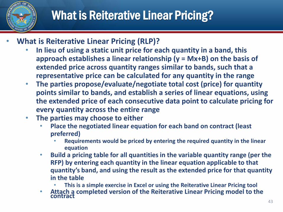
• What is Reiterative Linear Pricing (RLP)?• In lieu of using a static unit price for each quantity in a band, this
approach establishes a linear relationship (y = Mx+B) on the basis of extended price across quantity ranges similar to bands, such that a representative price can be calculated for any quantity in the range
• The parties propose/evaluate/negotiate total cost (price) for quantity points similar to bands, and establish a series of linear equations, using the extended price of each consecutive data point to calculate pricing for every quantity across the entire range
• The parties may choose to either • Place the negotiated linear equation for each band on contract (least
preferred)• Requirements would be priced by entering the required quantity in the linear
equation• Build a pricing table for all quantities in the variable quantity range (per the
RFP) by entering each quantity in the linear equation applicable to that quantity’s band, and using the result as the extended price for that quantity in the table • This is a simple exercise in Excel or using the Reiterative Linear Pricing tool
• Attach a completed version of the Reiterative Linear Pricing model to the contract
43
How to Construct Reiterative Linear Pricing
44
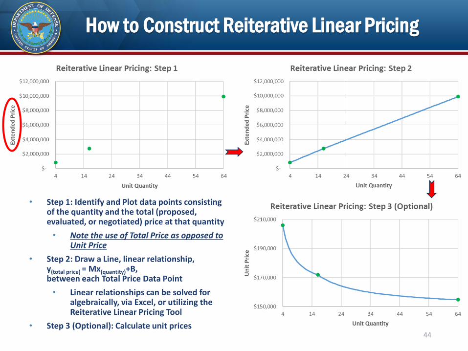
• Step 1: Identify and Plot data points consisting of the quantity and the total (proposed, evaluated, or negotiated) price at that quantity
• Note the use of Total Price as opposed to Unit Price
• Step 2: Draw a Line, linear relationship, y(total price) = Mx(quantity)+B, between each Total Price Data Point
• Linear relationships can be solved for algebraically, via Excel, or utilizing the Reiterative Linear Pricing Tool
• Step 3 (Optional): Calculate unit prices
How to Construct Using the Reiterative Linear Pricing Tool
45
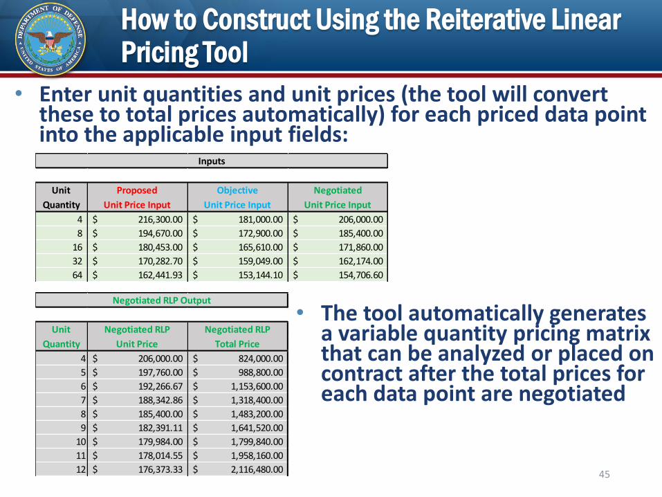
• Enter unit quantities and unit prices (the tool will convert these to total prices automatically) for each priced data point into the applicable input fields:
• The tool automatically generates a variable quantity pricing matrix that can be analyzed or placed on contract after the total prices for each data point are negotiated
Unit Negotiated RLP Negotiated RLP
Quantity Unit Price Total Price
4 206,000.00$ 824,000.00$
5 197,760.00$ 988,800.00$
6 192,266.67$ 1,153,600.00$
7 188,342.86$ 1,318,400.00$
8 185,400.00$ 1,483,200.00$
9 182,391.11$ 1,641,520.00$
10 179,984.00$ 1,799,840.00$
11 178,014.55$ 1,958,160.00$
12 176,373.33$ 2,116,480.00$
Negotiated RLP Output
Unit Proposed Objective Negotiated
Quantity Unit Price Input Unit Price Input Unit Price Input
4 216,300.00$ 181,000.00$ 206,000.00$
8 194,670.00$ 172,900.00$ 185,400.00$
16 180,453.00$ 165,610.00$ 171,860.00$
32 170,282.70$ 159,049.00$ 162,174.00$
64 162,441.93$ 153,144.10$ 154,706.60$
Inputs
How to Construct Using the Reiterative Linear Pricing Tool
46
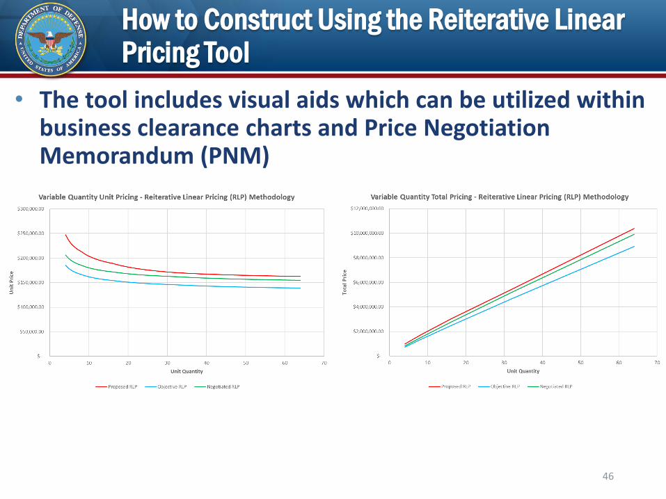
• The tool includes visual aids which can be utilized within business clearance charts and Price Negotiation Memorandum (PNM)
How to Construct Using the Reiterative Linear Pricing Tool
47
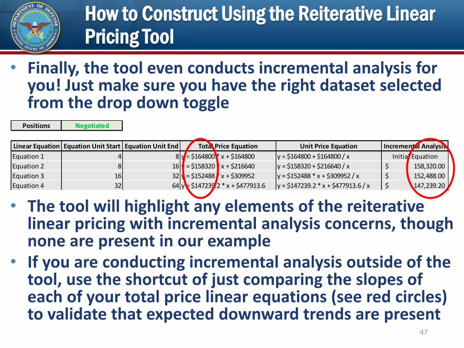
• Finally, the tool even conducts incremental analysis for you! Just make sure you have the right dataset selected from the drop down toggle
• The tool will highlight any elements of the reiterative linear pricing with incremental analysis concerns, though none are present in our example
• If you are conducting incremental analysis outside of the tool, use the shortcut of just comparing the slopes of each of your total price linear equations (see red circles) to validate that expected downward trends are present
Positions Negotiated
Linear Equation Equation Unit Start Equation Unit End Total Price Equation Unit Price Equation Incremental Analysis
Equation 1 4 8 y = $164800 * x + $164800 y = $164800 + $164800 / x Initial Equation
Equation 2 8 16 y = $158320 * x + $216640 y = $158320 + $216640 / x 158,320.00$
Equation 3 16 32 y = $152488 * x + $309952 y = $152488 * x + $309952 / x 152,488.00$
Equation 4 32 64 y = $147239.2 * x + $477913.6 y = $147239.2 * x + $477913.6 / x 147,239.20$
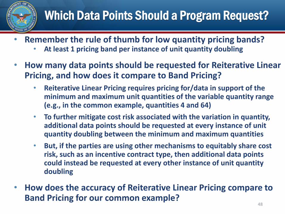
Which Data Points Should a Program Request?
• Remember the rule of thumb for low quantity pricing bands?• At least 1 pricing band per instance of unit quantity doubling
• How many data points should be requested for Reiterative Linear Pricing, and how does it compare to Band Pricing?
• Reiterative Linear Pricing requires pricing for/data in support of the minimum and maximum unit quantities of the variable quantity range (e.g., in the common example, quantities 4 and 64)
• To further mitigate cost risk associated with the variation in quantity, additional data points should be requested at every instance of unit quantity doubling between the minimum and maximum quantities
• But, if the parties are using other mechanisms to equitably share cost risk, such as an incentive contract type, then additional data points could instead be requested at every other instance of unit quantity doubling
• How does the accuracy of Reiterative Linear Pricing compare to Band Pricing for our common example?
48
Reiterative Linear Pricing vs Band Pricing
49
Reiterative Linear Pricing vs Band Pricing
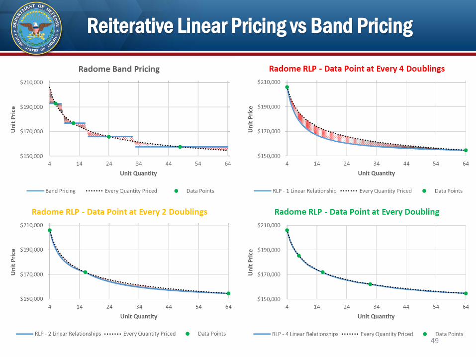
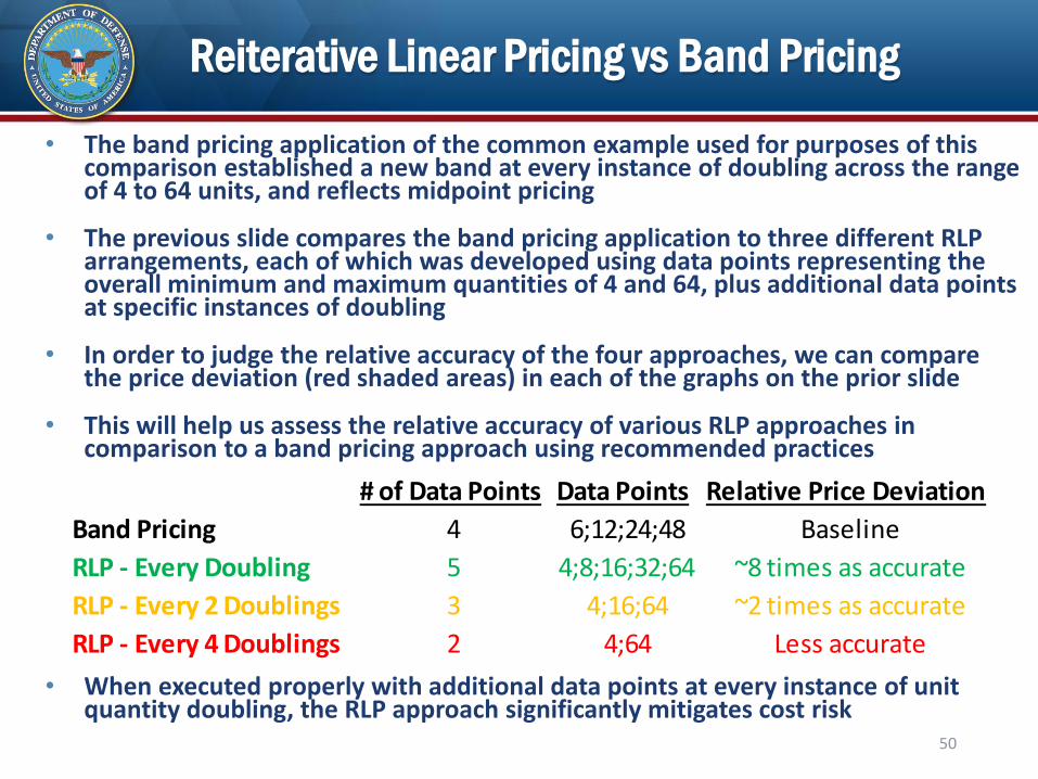
• The band pricing application of the common example used for purposes of this comparison established a new band at every instance of doubling across the range of 4 to 64 units, and reflects midpoint pricing
• The previous slide compares the band pricing application to three different RLP arrangements, each of which was developed using data points representing the overall minimum and maximum quantities of 4 and 64, plus additional data points at specific instances of doubling
• In order to judge the relative accuracy of the four approaches, we can compare the price deviation (red shaded areas) in each of the graphs on the prior slide
• This will help us assess the relative accuracy of various RLP approaches in comparison to a band pricing approach using recommended practices
• When executed properly with additional data points at every instance of unit quantity doubling, the RLP approach significantly mitigates cost risk
50
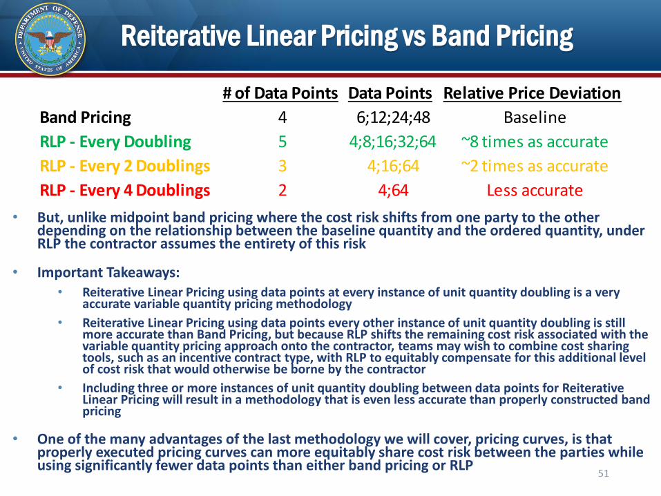
# of Data Points Data Points Relative Price Deviation
Band Pricing 4 6;12;24;48 Baseline
RLP - Every Doubling 5 4;8;16;32;64 ~8 times as accurate
RLP - Every 2 Doublings 3 4;16;64 ~2 times as accurate
RLP - Every 4 Doublings 2 4;64 Less accurate
Reiterative Linear Pricing vs Band Pricing
• But, unlike midpoint band pricing where the cost risk shifts from one party to the other depending on the relationship between the baseline quantity and the ordered quantity, under RLP the contractor assumes the entirety of this risk
• Important Takeaways:• Reiterative Linear Pricing using data points at every instance of unit quantity doubling is a very
accurate variable quantity pricing methodology
• Reiterative Linear Pricing using data points every other instance of unit quantity doubling is still more accurate than Band Pricing, but because RLP shifts the remaining cost risk associated with the variable quantity pricing approach onto the contractor, teams may wish to combine cost sharing tools, such as an incentive contract type, with RLP to equitably compensate for this additional level of cost risk that would otherwise be borne by the contractor
• Including three or more instances of unit quantity doubling between data points for Reiterative Linear Pricing will result in a methodology that is even less accurate than properly constructed band pricing
• One of the many advantages of the last methodology we will cover, pricing curves, is that properly executed pricing curves can more equitably share cost risk between the parties while using significantly fewer data points than either band pricing or RLP
51
# of Data Points Data Points Relative Price Deviation
Band Pricing 4 6;12;24;48 Baseline
RLP - Every Doubling 5 4;8;16;32;64 ~8 times as accurate
RLP - Every 2 Doublings 3 4;16;64 ~2 times as accurate
RLP - Every 4 Doublings 2 4;64 Less accurate
Pros & Cons of Reiterative Linear Pricing
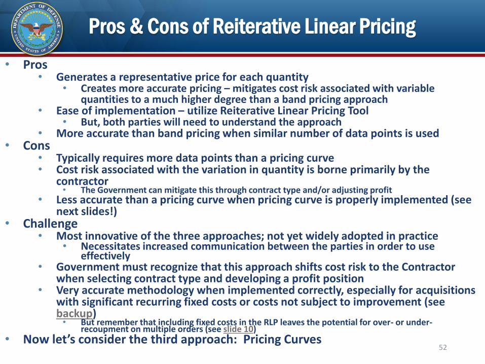
• Pros• Generates a representative price for each quantity
• Creates more accurate pricing – mitigates cost risk associated with variable quantities to a much higher degree than a band pricing approach
• Ease of implementation – utilize Reiterative Linear Pricing Tool• But, both parties will need to understand the approach
• More accurate than band pricing when similar number of data points is used• Cons
• Typically requires more data points than a pricing curve• Cost risk associated with the variation in quantity is borne primarily by the
contractor• The Government can mitigate this through contract type and/or adjusting profit
• Less accurate than a pricing curve when pricing curve is properly implemented (see next slides!)
• Challenge• Most innovative of the three approaches; not yet widely adopted in practice
• Necessitates increased communication between the parties in order to use effectively
• Government must recognize that this approach shifts cost risk to the Contractor when selecting contract type and developing a profit position
• Very accurate methodology when implemented correctly, especially for acquisitions with significant recurring fixed costs or costs not subject to improvement (see backup)• But remember that including fixed costs in the RLP leaves the potential for over- or under-
recoupment on multiple orders (see slide 10)• Now let’s consider the third approach: Pricing Curves
52
Approaches to Pricing Variable Quantities
Pricing Curves
53
What are Pricing Curves?
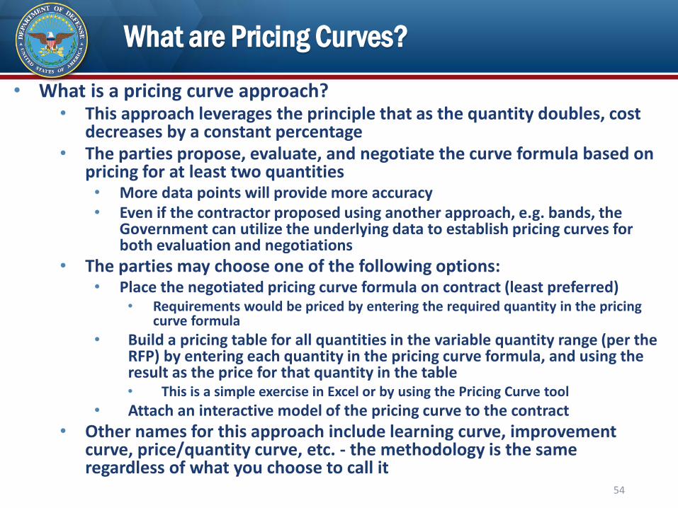
• What is a pricing curve approach?• This approach leverages the principle that as the quantity doubles, cost
decreases by a constant percentage• The parties propose, evaluate, and negotiate the curve formula based on
pricing for at least two quantities• More data points will provide more accuracy• Even if the contractor proposed using another approach, e.g. bands, the
Government can utilize the underlying data to establish pricing curves for both evaluation and negotiations
• The parties may choose one of the following options:• Place the negotiated pricing curve formula on contract (least preferred)
• Requirements would be priced by entering the required quantity in the pricing curve formula
• Build a pricing table for all quantities in the variable quantity range (per the RFP) by entering each quantity in the pricing curve formula, and using the result as the price for that quantity in the table • This is a simple exercise in Excel or by using the Pricing Curve tool
• Attach an interactive model of the pricing curve to the contract
• Other names for this approach include learning curve, improvement curve, price/quantity curve, etc. - the methodology is the same regardless of what you choose to call it
54
How to Construct a Pricing Curve
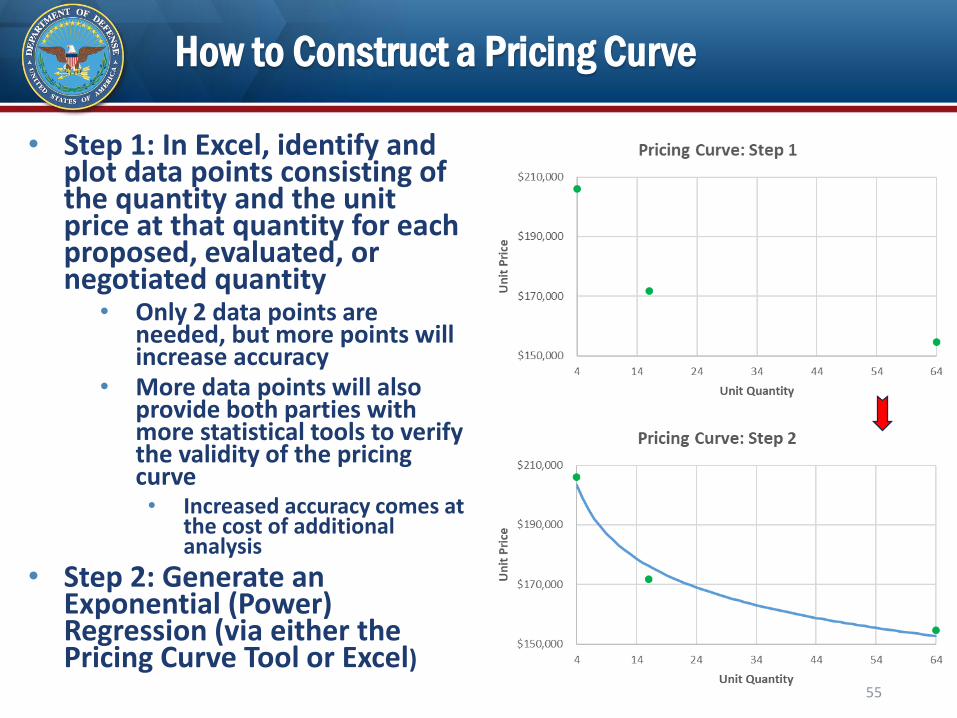
• Step 1: In Excel, identify and plot data points consisting of the quantity and the unit price at that quantity for each proposed, evaluated, or negotiated quantity
• Only 2 data points are needed, but more points will increase accuracy
• More data points will also provide both parties with more statistical tools to verify the validity of the pricing curve• Increased accuracy comes at
the cost of additional analysis
• Step 2: Generate an Exponential (Power) Regression (via either the Pricing Curve Tool or Excel)
55

Pricing Curve Equation
• The equation for a pricing curve is: y(unit price) = Mx(quantity)
B
• Y – Cost (price) of the Xth Unit (the dependent variable)
• M – The cost (price) of the theoretical first unit or T1
• X – The Xth Unit quantity (the independent variable)
• B – The logarithm, base 2, of the rate of improvement
• B can be rewritten as the following: B = log(z)/log(2)• z is the rate of improvement, expressed as a percentage• In other words, if you have an improvement rate of 90%,
B = log(90%)/log(2)• This rate would indicate that every time the unit quantity
doubles, the unit price will decrease by 10%
• As this equation captures only a single improvement rate (more on this in later charts), it is imperative that all fixed costs are segregated and separately priced
56
How to Construct Using the Pricing Curve Tool
57
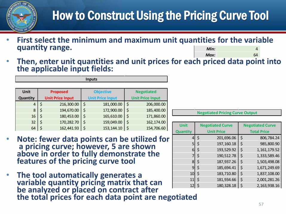
• First select the minimum and maximum unit quantities for the variable quantity range.
• Then, enter unit quantities and unit prices for each priced data point into the applicable input fields:
• Note: fewer data points can be utilized fora pricing curve; however, 5 are shown
above in order to fully demonstrate thefeatures of the pricing curve tool
• The tool automatically generates a variable quantity pricing matrix that can be analyzed or placed on contract afterthe total prices for each data point are negotiated
Min: 4
Max: 64
Unit Proposed Objective Negotiated
Quantity Unit Price Input Unit Price Input Unit Price Input
4 216,300.00$ 181,000.00$ 206,000.00$
8 194,670.00$ 172,900.00$ 185,400.00$
16 180,453.00$ 165,610.00$ 171,860.00$
32 170,282.70$ 159,049.00$ 162,174.00$
64 162,441.93$ 153,144.10$ 154,706.60$
Inputs
Unit Negotiated Curve Negotiated Curve
Quantity Unit Price Total Price
4 201,696.06$ 806,784.24$
5 197,160.18$ 985,800.90$
6 193,529.92$ 1,161,179.52$
7 190,512.78$ 1,333,589.46$
8 187,937.26$ 1,503,498.08$
9 185,694.41$ 1,671,249.69$
10 183,710.80$ 1,837,108.00$
11 181,934.66$ 2,001,281.26$
12 180,328.18$ 2,163,938.16$
Negotiated Pricing Curve Output
How to Construct Using the Pricing Curve Tool
58
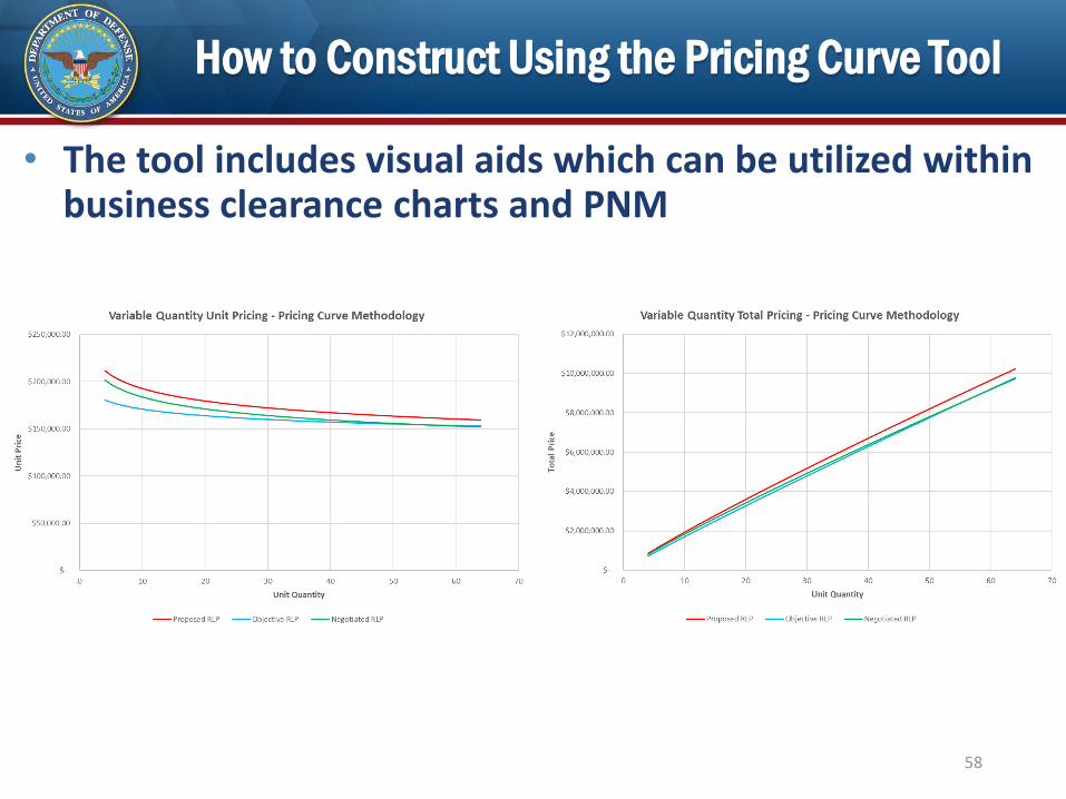
• The tool includes visual aids which can be utilized within business clearance charts and PNM
How to Construct Using the Pricing Curve Tool
59
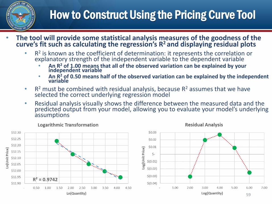
• The tool will provide some statistical analysis measures of the goodness of the curve’s fit such as calculating the regression’s R2 and displaying residual plots
• R2 is known as the coefficient of determination: it represents the correlation or explanatory strength of the independent variable to the dependent variable• An R2 of 1.00 means that all of the observed variation can be explained by your
independent variable• An R2 of 0.50 means half of the observed variation can be explained by the independent
variable
• R2 must be combined with residual analysis, because R2 assumes that we have selected the correct underlying regression model
• Residual analysis visually shows the difference between the measured data and the predicted output from your model, allowing you to evaluate your model’s underlying assumptions
How to Construct Using the Pricing Curve Tool
60
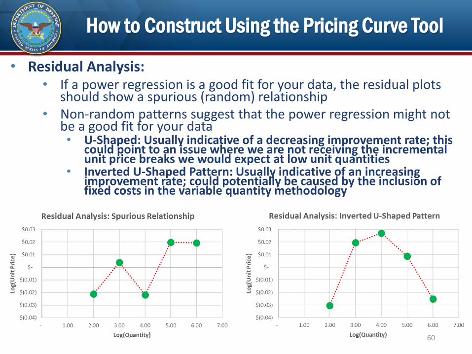
• Residual Analysis:• If a power regression is a good fit for your data, the residual plots
should show a spurious (random) relationship• Non-random patterns suggest that the power regression might not
be a good fit for your data• U-Shaped: Usually indicative of a decreasing improvement rate; this
could point to an issue where we are not receiving the incremental unit price breaks we would expect at low unit quantities
• Inverted U-Shaped Pattern: Usually indicative of an increasing improvement rate; could potentially be caused by the inclusion of fixed costs in the variable quantity methodology
How to Construct Using the Pricing Curve Tool
61
• What to do if you have a non-random residual pattern:
• First, determine the magnitude of the impact by comparing the input unit prices to the pricing curve’s predicted unit prices for those specific quantities• If the discrepancy is immaterial, no further evaluation needed
• Next, revisit your input unit prices• Conduct additional fact-finding to see if there are factors such as fixed
costs impacting your data• Modify and segregate inputs accordingly
• Finally, if the non-random residual pattern still presents a material discrepancy, consider modifying your variable quantity approach to better fit your input data• Note that the determination of materiality is a subjective assessment
that will need to be discussed by the two parties
Pricing Curve Considerations
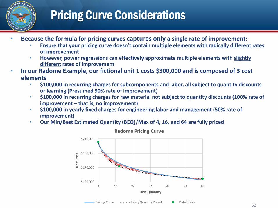
• Because the formula for pricing curves captures only a single rate of improvement:• Ensure that your pricing curve doesn’t contain multiple elements with radically different rates
of improvement• However, power regressions can effectively approximate multiple elements with slightly
different rates of improvement• In our Radome Example, our fictional unit 1 costs $300,000 and is composed of 3 cost
elements• $100,000 in recurring charges for subcomponents and labor, all subject to quantity discounts
or learning (Presumed 90% rate of improvement)• $100,000 in recurring charges for raw material not subject to quantity discounts (100% rate of
improvement – that is, no improvement)• $100,000 in yearly fixed charges for engineering labor and management (50% rate of
improvement)• Our Min/Best Estimated Quantity (BEQ)/Max of 4, 16, and 64 are fully priced
62
Pricing Curve Considerations
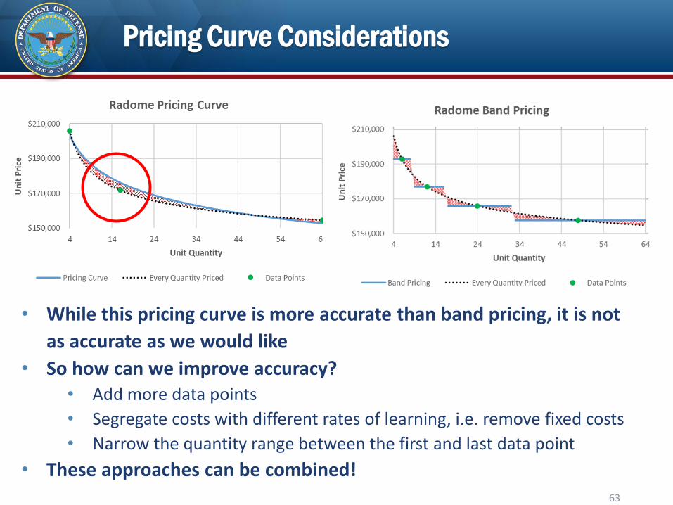
• While this pricing curve is more accurate than band pricing, it is not
as accurate as we would like
• So how can we improve accuracy?• Add more data points
• Segregate costs with different rates of learning, i.e. remove fixed costs
• Narrow the quantity range between the first and last data point
• These approaches can be combined!63
Pricing Curve: Number of Data Points
64
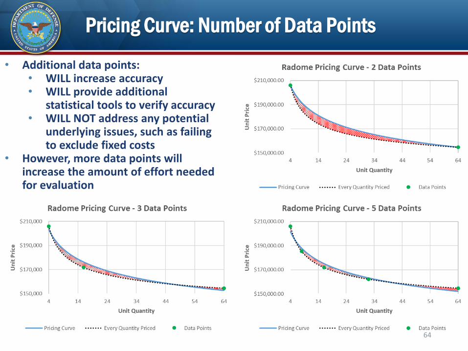
• Additional data points:• WILL increase accuracy• WILL provide additional
statistical tools to verify accuracy • WILL NOT address any potential
underlying issues, such as failing to exclude fixed costs
• However, more data points will increase the amount of effort needed for evaluation
Which Data Points Should a Program Request?
• Traditional 3 Data-Point Rule of Thumb: Min/BEQ/Max• 2 Data-Point Rule of Thumb: Likely Quantity Near Min / Likely
Quantity Near Max• Programs should consider their most likely non-BEQ quantities near the
min and max• Why spend resources analyzing quantities which all may have very low probabilities of
occurring?
• Both parties need to be aware of the potential drop-off in predictive accuracy before and after a Pricing Curve’s first and last evaluated data points• But remember, think logarithmically!• Increasing your minimum from 4 to 8 will have an impact on your pricing curve - you are
removing an instance of unit quantity doubling from your variable quantity range• Reducing your maximum from 64 to 60 might have little to no impact on your pricing
curve - reducing your maximum from 64 to 32 will have an impact because you are once again removing an instance of unit quantity doubling
• Ultimately, programs should ensure the points that are priced are representative of the pricing matrix range • Engage with your requirement owners and industry counterparts through market
research (competitive) or direct fact-finding (sole source) when determining what data points make the most sense
65
Pricing Curves: Narrowing the Data Points
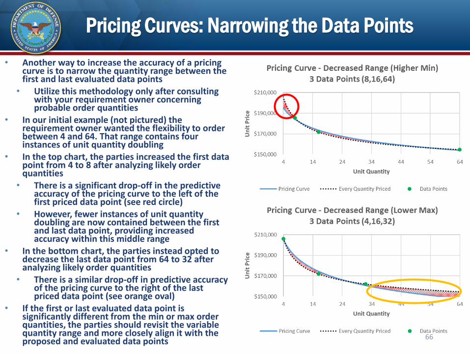
• Another way to increase the accuracy of a pricing curve is to narrow the quantity range between the first and last evaluated data points
• Utilize this methodology only after consulting with your requirement owner concerning probable order quantities
• In our initial example (not pictured) the requirement owner wanted the flexibility to order between 4 and 64. That range contains four instances of unit quantity doubling
• In the top chart, the parties increased the first data point from 4 to 8 after analyzing likely order quantities
• There is a significant drop-off in the predictive accuracy of the pricing curve to the left of the first priced data point (see red circle)
• However, fewer instances of unit quantity doubling are now contained between the first and last data point, providing increased accuracy within this middle range
• In the bottom chart, the parties instead opted to decrease the last data point from 64 to 32 after analyzing likely order quantities
• There is a similar drop-off in predictive accuracy of the pricing curve to the right of the last priced data point (see orange oval)
• If the first or last evaluated data point is significantly different from the min or max order quantities, the parties should revisit the variable quantity range and more closely align it with the proposed and evaluated data points
66
Pricing Curves: Segregating Costs
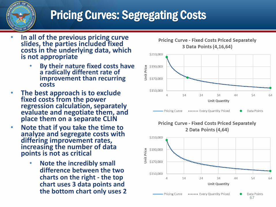
• In all of the previous pricing curve slides, the parties included fixed costs in the underlying data, which is not appropriate
• By their nature fixed costs have a radically different rate of improvement than recurring costs
• The best approach is to exclude fixed costs from the power regression calculation, separately evaluate and negotiate them, and place them on a separate CLIN
• Note that if you take the time to analyze and segregate costs with differing improvement rates, increasing the number of data points is not as critical
• Note the incredibly small difference between the two charts on the right - the top chart uses 3 data points and the bottom chart only uses 2
67
Pros & Cons of Pricing Curves
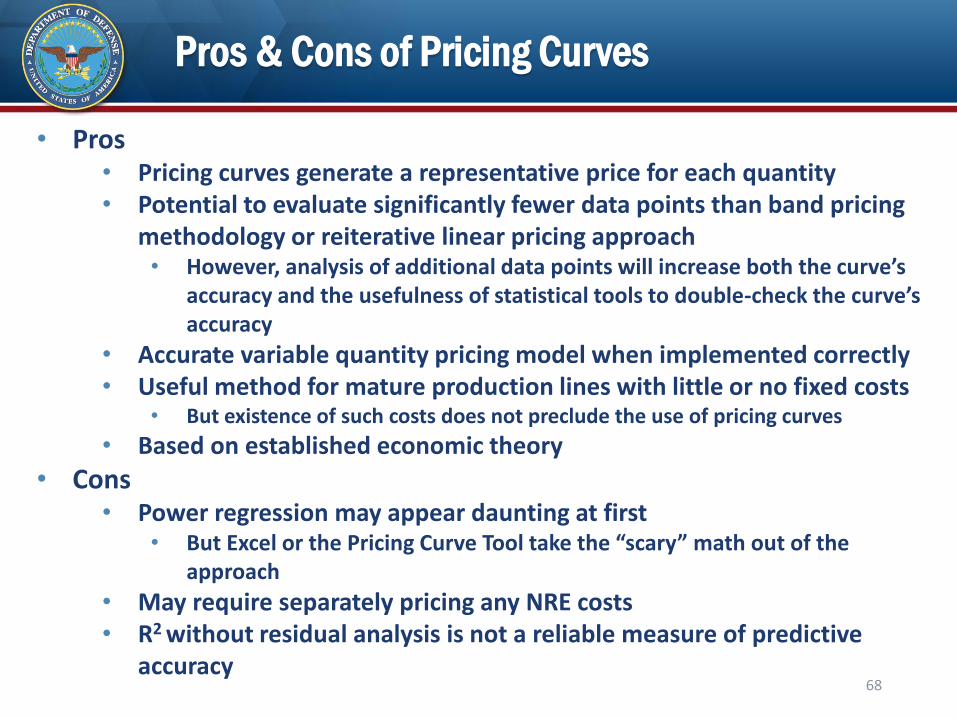
• Pros• Pricing curves generate a representative price for each quantity• Potential to evaluate significantly fewer data points than band pricing
methodology or reiterative linear pricing approach• However, analysis of additional data points will increase both the curve’s
accuracy and the usefulness of statistical tools to double-check the curve’s accuracy
• Accurate variable quantity pricing model when implemented correctly• Useful method for mature production lines with little or no fixed costs
• But existence of such costs does not preclude the use of pricing curves
• Based on established economic theory
• Cons• Power regression may appear daunting at first
• But Excel or the Pricing Curve Tool take the “scary” math out of the approach
• May require separately pricing any NRE costs• R2 without residual analysis is not a reliable measure of predictive
accuracy68
Approaches to Pricing Variable Quantities
Takeaways
69
When to use Variable Quantity Methodologies?
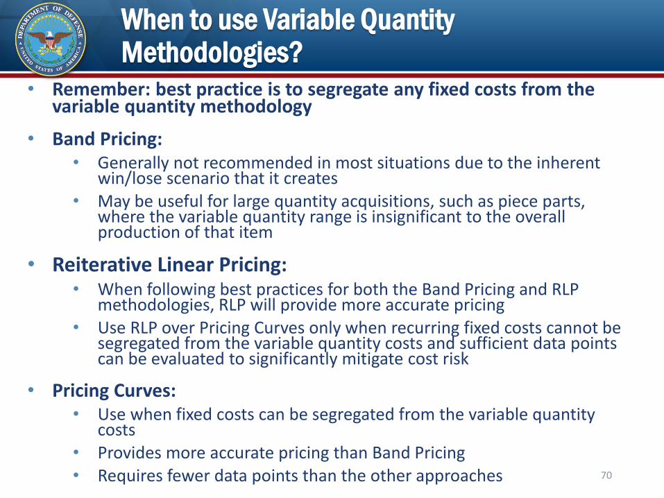
• Remember: best practice is to segregate any fixed costs from the variable quantity methodology
• Band Pricing:• Generally not recommended in most situations due to the inherent
win/lose scenario that it creates• May be useful for large quantity acquisitions, such as piece parts,
where the variable quantity range is insignificant to the overall production of that item
• Reiterative Linear Pricing:• When following best practices for both the Band Pricing and RLP
methodologies, RLP will provide more accurate pricing• Use RLP over Pricing Curves only when recurring fixed costs cannot be
segregated from the variable quantity costs and sufficient data points can be evaluated to significantly mitigate cost risk
• Pricing Curves:• Use when fixed costs can be segregated from the variable quantity
costs• Provides more accurate pricing than Band Pricing• Requires fewer data points than the other approaches 70
Common Threads
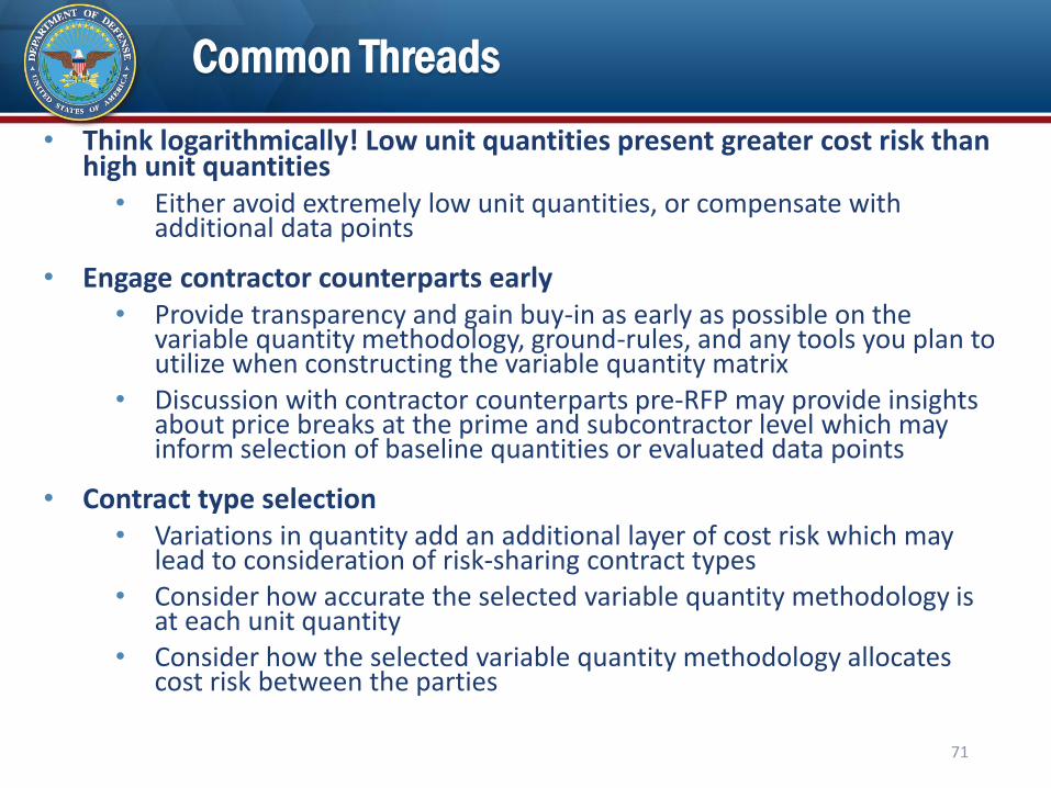
• Think logarithmically! Low unit quantities present greater cost risk than high unit quantities
• Either avoid extremely low unit quantities, or compensate with additional data points
• Engage contractor counterparts early• Provide transparency and gain buy-in as early as possible on the
variable quantity methodology, ground-rules, and any tools you plan to utilize when constructing the variable quantity matrix
• Discussion with contractor counterparts pre-RFP may provide insights about price breaks at the prime and subcontractor level which may inform selection of baseline quantities or evaluated data points
• Contract type selection• Variations in quantity add an additional layer of cost risk which may
lead to consideration of risk-sharing contract types• Consider how accurate the selected variable quantity methodology is
at each unit quantity• Consider how the selected variable quantity methodology allocates
cost risk between the parties
71
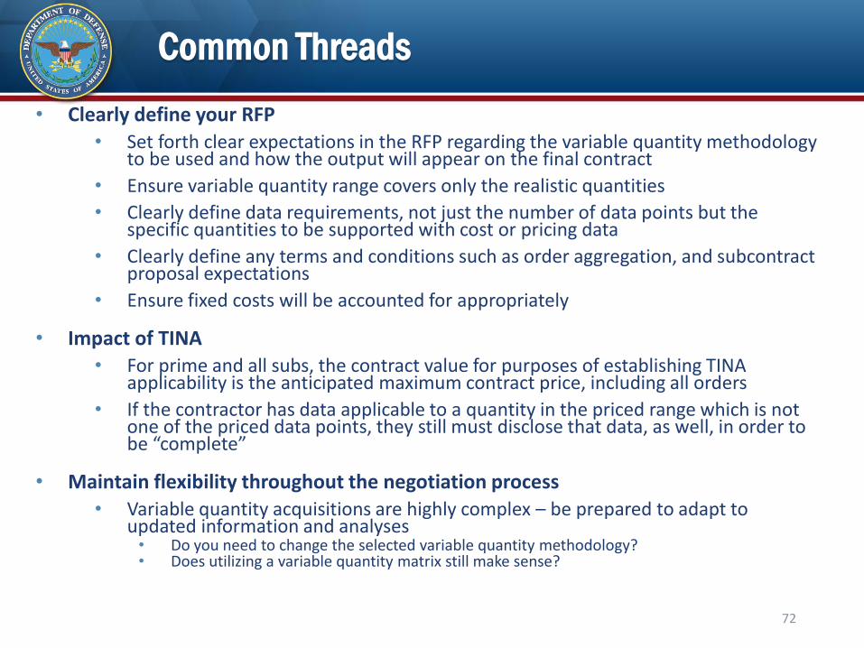
Common Threads
• Clearly define your RFP• Set forth clear expectations in the RFP regarding the variable quantity methodology
to be used and how the output will appear on the final contract
• Ensure variable quantity range covers only the realistic quantities
• Clearly define data requirements, not just the number of data points but the specific quantities to be supported with cost or pricing data
• Clearly define any terms and conditions such as order aggregation, and subcontract proposal expectations
• Ensure fixed costs will be accounted for appropriately
• Impact of TINA• For prime and all subs, the contract value for purposes of establishing TINA
applicability is the anticipated maximum contract price, including all orders
• If the contractor has data applicable to a quantity in the priced range which is not one of the priced data points, they still must disclose that data, as well, in order to be “complete”
• Maintain flexibility throughout the negotiation process• Variable quantity acquisitions are highly complex – be prepared to adapt to
updated information and analyses• Do you need to change the selected variable quantity methodology?• Does utilizing a variable quantity matrix still make sense?
72
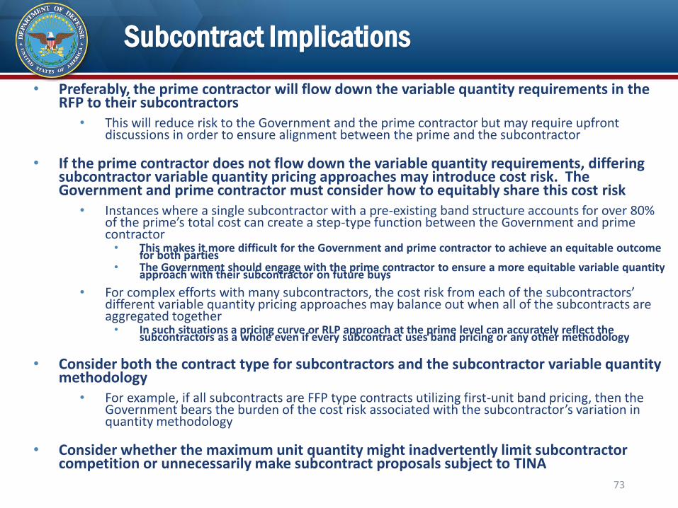
Subcontract Implications
• Preferably, the prime contractor will flow down the variable quantity requirements in the RFP to their subcontractors
• This will reduce risk to the Government and the prime contractor but may require upfront discussions in order to ensure alignment between the prime and the subcontractor
• If the prime contractor does not flow down the variable quantity requirements, differing subcontractor variable quantity pricing approaches may introduce cost risk. The Government and prime contractor must consider how to equitably share this cost risk
• Instances where a single subcontractor with a pre-existing band structure accounts for over 80% of the prime’s total cost can create a step-type function between the Government and prime contractor • This makes it more difficult for the Government and prime contractor to achieve an equitable outcome
for both parties• The Government should engage with the prime contractor to ensure a more equitable variable quantity
approach with their subcontractor on future buys
• For complex efforts with many subcontractors, the cost risk from each of the subcontractors’ different variable quantity pricing approaches may balance out when all of the subcontracts are aggregated together• In such situations a pricing curve or RLP approach at the prime level can accurately reflect the
subcontractors as a whole even if every subcontract uses band pricing or any other methodology
• Consider both the contract type for subcontractors and the subcontractor variable quantity methodology
• For example, if all subcontracts are FFP type contracts utilizing first-unit band pricing, then the Government bears the burden of the cost risk associated with the subcontractor’s variation in quantity methodology
• Consider whether the maximum unit quantity might inadvertently limit subcontractor competition or unnecessarily make subcontract proposals subject to TINA
73
Resources
• DAU Cost Improvement (Prediction Interval) Template
• Upcoming DAU Virtual Learning Workshop CON 7420V • Scheduled to be piloted in November 2021• Will address learning curves in detail
• Contract Pricing Reference Guides, Volume 2, Ch. 7
• Pricing Curve Tool
• Reiterative Linear Pricing Tool
• Many 3rd party websites provide helpful resources for regressions and statistical analysis
• Example 3rd Party Pricing Curve (Power Regression) Resources:• https://www.statology.org/power-regression-in-excel/
• Example 3rd Party Residual Analysis Resource:• https://opexresources.com/analysis-residuals-explained/
• These 3rd party links are provided for informational purposes only and do not constitute an endorsement, an approval, or an assumption of responsibility by the Government
74

Questions?
75

Backup
76
Terminology
• BEQ: Best Estimated Quantity, the quantity most likely to be ordered
• Extended Price Analysis
• Incremental Unit Analysis
• Linear Regression: y = Mx + B
• Power Regression: y = Mx^B
• Pricing Table / Variable Quantity Matrix: A numerical table that displays the relationship between quantity, unit price, and total price for all quantities within the variable quantity range.
• Residual Analysis
77
Pricing Curve Final Thoughts
• It is possible to fully conduct statistical analysis and fact-finding yet arrive in a situation where a traditional pricing curve does not provide a materially accurate enough result
• In such situations consider the following mitigation strategies:
• Employ a series of correction factors, based off of the residual price (difference between analyzed and predicted) for analyzed quantities• This methodology can be accomplished in the Pricing Curve Tool
• Instead of using a single pricing curve, consider applying multiple curves in a style similar to RLP’s use of linear regressions.
• Independently model individual cost element inputs, then aggregate to calculate the unit prices across the variable quantity range
• As a last resort, consider switching to RLP if you have sufficient data points
• All of the above strategies assume that earlier best practices were followed, including proper segregation of fixed costs, and a robust evaluation of the data points has been performed
78
Pricing Curve vs Reiterative Linear Pricing: Fixed Costs
• If you can separately price fixed costs, use a Pricing Curve
• Remember, separating fixed costs is a best practice!
• If you can’t separately price fixed costs, use Reiterative Linear Pricing
• If fixed costs cannot be segregated, be aware of how your potential order practices could result in over- or under-recoupment of fixed costs
• So how does this work mathematically?
• Pricing Curves: Can flexibly approximate any single rate of improvement• Math: Y(unit) = Mx^(log(z)/log(2) Note the single improvement rate, z, in the
pricing curve formula
• Reiterative Linear Pricing: Approximates two rates of improvement, but those rates are always constant• Math: y(total) = Mx+B• Thanks to algebra, this can be rewritten and translated into the following unit
price equation: Y(unit) = Mx^(log(100%)/log(2)) + Bx^(log(50%)/log(2))• Interestingly, Reiterative Linear Pricing provides two distinct improvement rates
that happen to mimic non-recurring (50% improvement) and fixed costs (100% improvement) in a variable quantity relationship
79
Addressing Fixed Costs in your Acquisition
• Remember, fixed costs are expenses that are constant regardless of quantity; they can be either recurring or non-recurring
• Recurring fixed costs are often tied to the passage of time, but not always
• Other common variables that might have associated recurring fixed costs:• Number of customers• Production throughput• Number of orders placed
• Remember, best practice is to always segregate fixed costs
• These costs should then be recognized at the rate they are incurred (a single time; once per order, regardless of order quantity; once per year, etc.)
• Potential Approaches:
• First order/customer bears 100% of the fixed costs
• Attempt to amortize fixed costs across multiple orders• Example: If you have $100m in projected fixed costs and believe you will place 4
orders, each order should be responsible for $25m in projected fixed costs• But, be aware of how your other potential order practices could result in over-
or under-recoupment of fixed costs
80


