Primary User Activity Modeling Using First-Difference Filter Clustering and Correlation in Cognitive...

170 IEEE/ACM TRANSACTIONS ON NETWORKING, VOL. 19, NO. 1, FEBRUARY 2011

Primary User Activity Modeling UsingFirst-Difference Filter Clustering and

Correlation in Cognitive Radio NetworksBerk Canberk, Student Member, IEEE, Ian F. Akyildiz, Fellow, IEEE, Fellow, ACM, and Sema Oktug, Member, IEEE

Abstract—In many recent studies on cognitive radio (CR) net-works, the primary user activity is assumed to follow the Poissontraffic model with exponentially distributed interarrivals. ThePoisson modeling may lead to cases where primary user activitiesare modeled as smooth and burst-free traffic. As a result, this maycause the cognitive radio users to miss some available but unuti-lized spectrum, leading to lower throughput and high false-alarmprobabilities. The main contribution of this paper is to proposea novel model to parametrize the primary user traffic in a moreefficient and accurate way in order to overcome the drawbacksof the Poisson modeling. The proposed model makes this possibleby arranging the first-difference filtered and correlated primaryuser data into clusters. In this paper, a new metric called thePrimary User Activity Index, �, is introduced, which accountsfor the relation between the cluster filter output and correlationstatistics. The performance of the proposed model is evaluatedby means of traffic estimation accuracy, false-alarm probabilitieswhile keeping the detection probability of primary users at aconstant value. Simulation results show that the appropriateselection of the Primary User Activity Index, higher primary-userdetection accuracy, reduced false-alarm probabilities, and higherthroughput can be achieved by the proposed model.

Index Terms—Clustering, cognitive radio (CR) networks, pri-mary user activity modeling.

I. INTRODUCTION

I N COGNITIVE radio (CR) networks, primary users (PUs)are defined as wireless devices that have the license to op-

erate in a specific spectrum band. Since PUs have priority toutilize the licensed spectrum, their communication should notbe interrupted or interfered with any other users. However, CRusers are supposed to sense the spectrum and utilize the unused

Manuscript received December 31, 2008; revised December 20, 2009;accepted June 20, 2010; approved by IEEE/ACM TRANSACTIONS ON

NETWORKING Editor M. Buddhikot. Date of publication August 19, 2010; dateof current version February 18, 2011. This work was supported by the IstanbulChamber of Industry (ISO). The work of I. F. Akyildiz was supported by theU.S. National Science of Foundation under Award CNS-0721580.

B. Canberk was with the Broadband Wireless Networking Laboratory(BWNLab), School of Electrical and Computer Engineering, GeorgiaInstitute of Technology, Atlanta, GA 30332 USA. He is now with the De-partment of Computer Engineering, Faculty of Electrical and ElectronicEngineering, Istanbul Technical University, 34469 Istanbul, Turkey (e-mail:[email protected]).

I. F. Akyildiz is with the Broadband Wireless Networking Laboratory(BWNLab), School of Electrical and Computer Engineering, Georgia Instituteof Technology, Atlanta, GA 30332 USA (e-mail: [email protected]).

S. Oktug is with the Department of Computer Engineering, Faculty of Elec-trical and Electronic Engineering, Istanbul Technical University, 34469 Istanbul,Turkey (e-mail: [email protected]).

Digital Object Identifier 10.1109/TNET.2010.2065031

bands in an opportunistic manner. CR users may occupy avail-able bands as long as the corresponding PU is active, but mustimmediately evacuate the band as soon as the corresponding PUappears [1].

CR users should intelligently determine the ongoing PU ac-tivities in a licensed spectrum band to avoid interference withthe PUs [1]. Moreover, the PU activities need to be accuratelymodeled so that CR users can evacuate the band without af-fecting PU activities. CR users also need to detect spectrumholes to identify transmission opportunities so that the spectrumusage is maximized [2]. Hence, it could be stated that preciseestimations/modeling of PU activities leads to much more ef-fective spectrum usage for CR users.

In recent studies, the PU activity is assumed to follow thePoisson model [3]–[6]. However, the Poisson model fails incapturing the bursty and spiky characteristics of the monitoreddata [2], [7], [8]. As a result, the existing works based on thePoisson model consider the PU activities as smooth and burst-free, in which short-term fluctuations are neglected. Moreover,some large-scale measurement-driven characterizations of thePU activities in cellular networks are also carried out for dif-ferent spectrum bands. In [9], the authors analyze the spec-trum occupancy of PUs in GSM and UMTS bands. In [10], thePU activities are analyzed in the New York cellular bands, i.e.,CDMA and GSM. In [11], the authors analyze the call logs of aswitch of a cellular GSM provider in Qingdao, China. In [2], itis pointed out that the PU activity durations are nonexponentialand changes in time scale violating the Poisson assumptions. Itwas also pointed out that the spectrum usage of PUs fluctuatessignificantly even with a few seconds, hence CR users must beaware of these short-term fluctuations. Note that the PU activitymodels in that work are based on long-term observations.

Overall, the Poisson model approximates the PU activities assmooth and burst-free traffic. Though the PU activity exhibitsshort-term temporal diversity, i.e., significant and spiky fluctua-tions over time, these variations are not captured by the Poissonmodel, as shown in Fig. 1. The model represents the ON period,i.e., the active transmission duration of a PU, by the horizontallevel at constant amplitude of dBm. The OFF period, whichrepresents the absence of PU activity, is also given by the con-stant amplitude of dBm. It could be observed that the actualPU activity fluctuates during the ON period, which is not exactlytracked by the Poisson model. Some of these fluctuations re-sult in durations, where the PU is actually absent, shown by thedashed lines. These durations, which are classified as a part ofthe ON period by the Poisson model, cause missed transmission

1063-6692/$26.00 © 2010 IEEE

CANBERK et al.: PU ACTIVITY MODELING USING FIRST-DIFFERENCE FILTER CLUSTERING AND CORRELATION IN CR NETWORKS 171

Fig. 1. Missed transmission opportunities caused by the Poisson modeling.

opportunities for the CR users. The Poisson model is incapableof identifying fluctuations. This leads to fewer cases of correctspectrum hole detection, thus causing a degradation in CR net-work performance.

In this paper, we introduce a novel PU activity model ad-dressing the potential drawbacks of the Poisson modeling withthe following contributions.

• A new PU activity detection technique based on the First-Difference Clustering scheme is introduced.

• A new temporal correlation-based PU activity modelingscheme in order to detect the spectrum holes in a band isproposed.

• The PU activity detection and the spectrum hole detec-tion schemes are combined to maximize the CR networkperformance.

In this work, spiky and bursty PU activities are captured moreaccurately. Moreover, a new parameter called the Primary UserActivity Index (the PU activity index), , is introduced to pa-rametrize the PU activities as well as the spectrum holes. Fi-nally, the overall CR network performance, in terms of estima-tion accuracy, false-alarm probabilities, and throughput is eval-uated under different -values.

The rest of the paper is organized as follows. In Section II,the overview of the network architecture and the model we pro-posed are described. In Section III, we explain the Clustering-Modeling Module by giving details of the proposed PU activitymodeling. In Section IV, the performance of the proposed modelis evaluated in terms of traffic estimation, false-alarm probabil-ities, and throughput. In Section V, we conclude the paper bysummarizing the achievements and giving future directions.

II. NETWORK ARCHITECTURE AND PROPOSED MODEL

We consider an infrastructure-based CR network architectureintegrated in a PU network that has the license to operate ina certain spectrum band [4]. Moreover, the CR network has acentralized network entity such as a base station and associatedCR users. Each CR user monitors the spectrum band and sendsits local observations, i.e., the monitored PU activities, to thebase station, which broadcasts the PU activity model to the CRusers.

Fig. 2. Block diagram of the proposed model.

TABLE IKEY NOTATIONS

The model we propose consists of two main modules: thePU Activity Monitoring Module and the Clustering-ModelingModule, which are illustrated in Fig. 2. The notations used arelisted in Table I.

The PU Activity Monitoring Module, which is implementedin each CR user, monitors the spectrum band and samples thePU activity. We use the following noncooperative spectrumsensing scheme at each CR user [3], [12]:

(1)

where is the th sample of the monitored PU activityvector , which is sampled at the sampling frequency anddefined as

(2)

where is the total number of PU monitored activity samples.Moreover, and in (1) are the hypotheses that indicate ei-ther the PU does not have an activity or does have an activityin the spectrum band, respectively. In addition, in (1) rep-resents the additive white Gaussian noise (AWGN) with zeromean and variance , and is the primaryuser’s unknown signal, which is an independent and identicallydistributed (iid) random process with mean and variance

as in [13]. It is also assumed that and


are independent. Thus, the signal-to-noise ratio (SNR) isgiven by .

Once the monitoring is finished, the PU Activity MonitoringModule gives the monitored PU activity vector for modelingand analysis to the Clustering-Modeling Module, which is im-plemented in the base station. The Clustering-Modeling Moduleactivates its Clustering Engine, where the monitored PU activitysamples are accumulated into clusters using a first-difference fil-tering procedure enhanced with temporal correlation. As a re-sult, a new PU activity vector with clusters is generated andthen input to the Modeling Engine as seen in Fig. 2. In this en-gine, a correlation-based modeling scheme produces the newmodeled PU activity and parametrizes PU activity characteris-tics, i.e., producing , the probability of PU absence, and

, the probability of PU presence. The details of the Clus-tering-Modeling Module are given in Section III.

The newly generated PU activity characteristics and the mod-eled PU activity vector are fed back to the CR user. Here, themodeled PU activity is input to the energy detector to be usedfor spectrum sensing. Since the energy detector gets samples ofsize , it completes the operation in iterations. At the endof the operation, the energy detector triggers the PU ActivityMonitoring Module using the local clock for a new analysis.

In the model, we use the maximum a posteriori (MAP) en-ergy detection, i.e., the a posteriori PU activity probabilities,which could be summarized as follows [3], [13]. The energydetector consists of a bandpass filter, a squaring module, an in-tegrator, and a decision maker. The energy of the received signalis bandpassed by the filter with bandwidth . The output signalof this bandpass filter is squared and integrated over the sensingtime . The output of the integrator is compared to a threshold

in the decision maker to decide whether the PU is present ornot.

The output of the integrator follows the chi-square distribu-tion [13]. When the number of samples is large, the output canbe approximated by Gaussian distribution using central limittheorem [14]. Therefore, the false-alarm probability and thedetection probability can be evaluated by considering PU ac-tivity characteristics as [3]

(3)

(4)

where is the th sample of , which is the modeled PU ac-tivity vector , which is smaller than or equal to gives thenumber of samples; is the sensing time; is the completeGamma function; is the incomplete Gamma function;and is the generalized Marcum Q-function.

Moreover, the proposed model calculates the maximumachievable throughput of a CR user as in [15]

(5)

where is the total frame duration, and is thethroughput of a CR user without PU existence. is equal to

Fig. 3. Flowchart of the clustering engine.

, where is the received power of the CR userand is the noise power.

III. CLUSTERING-MODELING MODULE

The Clustering-Modeling Module has two engines to processthe monitored PU activity: the Clustering Engine and the Mod-eling Engine, as shown in Fig. 2. The details of the engines areexplained.

A. Clustering Engine

The Clustering Engine works based on the flow diagramgiven in Fig. 3.

When the PU Activity Monitoring Module gives the moni-tored PU activity vector to the Clustering-Modeling Module,it activates its Clustering Engine. Here, the monitored PU ac-tivity samples are accumulated into clusters. A cluster is a vectorwhere PU activity samples are accumulated according to somehypothesis tests. We introduce the notation to express the

th cluster. In a cluster , the PU samples are assumed to behomogeneous. We exploit this homogeneity for more accuratedetection of PU activities. Since all samples in the th clusterhave same power level, the energy detector, shown in Fig. 2,results with the same decision for them, leading to a more accu-rate detection as long as the samples within a cluster are highlycorrelated.

In this engine, the monitored PU activity samples are clus-tered using a first-difference filtering procedure enhanced withtemporal correlation. The details of the first-difference filteringare given in Appendix A. As a result, a new PU activity vectorwith clusters is generated and then input to the ModelingEngine.

At the beginning of the clustering process, the Clustering En-gine receives the monitored PU activity vector from the PUActivity Monitoring Module and sets , indicating the


start index of the monitored PU activity vector; the cluster index, representing the first cluster; and the randomly predeter-

mined parameters , the clustering parameter (detailed inAppendix A), and , the correlation parameter (detailed inAppendix B), for . Since the monitored PU activityis input to the Clustering Engine Module, we may assume thatthe modeled PU activity vector is identical to the monitoredPU activity vector input to the Clustering Engine, i.e., .Then, all the consecutive samples (the current sample andthe last sample ) are passed through the first-differencefinite-impulse response (FIR) filter [detailed in Appendix A andcalculated in (38)]. In the next step, the filter output ischecked with a -test (detailed in Appendix A). If the -test issuccessful, the -test (detailed in Appendix B) is applied. Con-sequently, the modeled PU activity sample is placed in theexisting cluster with its predecessor if bothtests are successful, whereas any fail from these two tests leadsthe sample to form a new cluster . This processis repeated until all the samples in the monitored PU activityvector are analyzed. Then, the clustered PU activity vector ofsize is formed by mean values of each cluster.

As a result, only the modeled PU activity sample , whichis close to its predecessor (successful in -test) andhighly correlated with the last two samples ,(successful in -test), is placed in the same cluster with its pre-decessor . By using clustering, groups of first-differ-ence filtered PU activity samples that have different correlationstatistics are separated. In other words, spiky and bursty char-acteristics of the modeled PU activity are more accurately dis-tinguished by employing clustering, which leads the CR user todetect the PU activity fluctuations more precisely, hence causingless interference.

B. Modeling Engine

The Modeling Engine produces a correlation-based modelingscheme in order to parametrize the PU activity characteristics.The operations performed in this engine have a flow diagramshown in Fig. 4.

At the Modeling Engine, and are set to 1 and the israndomly predetermined for . After this preprocessing,the Modeling Engine enters the loop until all samples are ex-ecuted. At each run, the engine determines a decision regionusing Table III for the pair of clusters amongfour regions. Decision regions are defined for a pair of clusters

, and each pair can reach only one of the re-gions at the end of the Modeling Engine. Moreover, the regionsare expressed by different combinations of the two binary vari-ables and , which are defined in Table II. The two binaryvariables and are employed to mathematically express the

-test [detailed in Appendix A and given in (47)] and the corre-lation slope test [detailed in Appendix B and given in (50)], re-spectively. More precisely, the variables and take the value1 under a certain hypothesis, and 0 if the hypothesis is not true.These variables and their hypotheses are expressed in Table II.As seen in Table II, the variable represents that the -testin (47), which is realized in the Modeling Engine, is successful

. The , which is the complementof , represents that the -test in (47) failed. Moreover, the

Fig. 4. Flowchart of the modeling engine.

TABLE IIVARIABLES �, � AND THEIR HYPOTHESES

variable in Table II is used when the correlation slopetest, calculated in the Modeling Engine using (50), is positive

. The , which is the complementary

of , shows that the result of (50) is negative.At each decision region, there are two possible decisions that

the clusters and can take. These are and. means that the clusters are modeled as the ab-

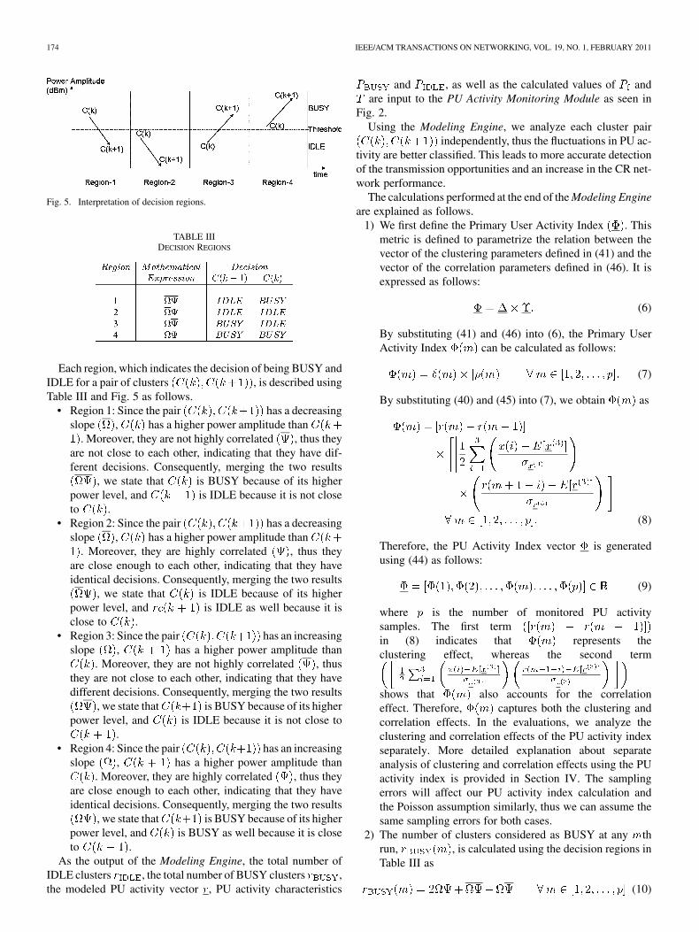
sence of PU activity, whereas indicates that the clus-ters are modeled as the existence of PU activity. The regions,their mathematical expressions, and the decisions for the clusterpair at each region are shown in Table III.In addition, the interpretation of each decision region for thecluster pair is illustrated in Fig. 5. Note thatthe threshold value in Fig. 5 is selected as the mean power ofthe monitored PU activity, and is the cluster index.


Fig. 5. Interpretation of decision regions.

TABLE IIIDECISION REGIONS

Each region, which indicates the decision of being BUSY andIDLE for a pair of clusters , is described usingTable III and Fig. 5 as follows.

• Region 1: Since the pair has a decreasingslope , has a higher power amplitude than

. Moreover, they are not highly correlated , thus theyare not close to each other, indicating that they have dif-ferent decisions. Consequently, merging the two results

, we state that is BUSY because of its higherpower level, and is IDLE because it is not closeto .

• Region 2: Since the pair has a decreasingslope , has a higher power amplitude than

. Moreover, they are highly correlated , thus theyare close enough to each other, indicating that they haveidentical decisions. Consequently, merging the two results

, we state that is IDLE because of its higherpower level, and is IDLE as well because it isclose to .

• Region 3: Since the pair has an increasingslope , has a higher power amplitude than

. Moreover, they are not highly correlated , thusthey are not close to each other, indicating that they havedifferent decisions. Consequently, merging the two results

, we state that is BUSY because of its higherpower level, and is IDLE because it is not close to

.• Region 4: Since the pair has an increasing

slope , has a higher power amplitude than. Moreover, they are highly correlated , thus they

are close enough to each other, indicating that they haveidentical decisions. Consequently, merging the two results

, we state that is BUSY because of its higherpower level, and is BUSY as well because it is closeto .

As the output of the Modeling Engine, the total number ofIDLE clusters , the total number of BUSY clusters ,the modeled PU activity vector , PU activity characteristics

and , as well as the calculated values of andare input to the PU Activity Monitoring Module as seen in

Fig. 2.Using the Modeling Engine, we analyze each cluster pair

independently, thus the fluctuations in PU ac-tivity are better classified. This leads to more accurate detectionof the transmission opportunities and an increase in the CR net-work performance.

The calculations performed at the end of the Modeling Engineare explained as follows.

1) We first define the Primary User Activity Index . Thismetric is defined to parametrize the relation between thevector of the clustering parameters defined in (41) and thevector of the correlation parameters defined in (46). It isexpressed as follows:

(6)

By substituting (41) and (46) into (6), the Primary UserActivity Index can be calculated as follows:

(7)

By substituting (40) and (45) into (7), we obtain as

(8)

Therefore, the PU Activity Index vector is generatedusing (44) as follows:

(9)

where is the number of monitored PU activitysamples. The first termin (8) indicates that represents theclustering effect, whereas the second term

shows that also accounts for the correlationeffect. Therefore, captures both the clustering andcorrelation effects. In the evaluations, we analyze theclustering and correlation effects of the PU activity indexseparately. More detailed explanation about separateanalysis of clustering and correlation effects using the PUactivity index is provided in Section IV. The samplingerrors will affect our PU activity index calculation andthe Poisson assumption similarly, thus we can assume thesame sampling errors for both cases.

2) The number of clusters considered as BUSY at any thrun, , is calculated using the decision regions inTable III as

(10)


where is the number of monitored PU activity samples.This three-term equation can be retrieved from the flow di-agram given in Fig. 4 by following logical paths to reachregions 4, 1, and 3, which are defined in Table III, respec-tively. They are combined by the logical expressionsince a pair of clusters can reside onlyin one of the three available regions. in the first termof (10) shows that . Besides,and are highly correlated because of . Since thesetwo variables are highly correlated in an increasing rela-tionship, they are both considered as BUSY at region 4(the number 2 in the first term). Therefore, the result is

. Looking at the second term of (10), one cansee that and are in a decreasing trend ,and they are not highly correlated , henceis IDLE whereas is BUSY at region 1. Therefore,the result is . The third term of (10) indi-cates that and are in an increasing rela-tionship and they are not highly correlated , thus

is BUSY and is IDLE at region 3. As a re-sult, .

3) The number of clusters considered as IDLE at any thrun, , is calculated using the decision regions inTable III as

(11)

This three-term equation can also be retrieved from theflow diagram given in Fig. 4 by following the logical pathsto reach regions 2, 1, and 3, which are defined in Table III,respectively. Using the decision regions in Table III, we seethat in regions 1 and 3, whereas inregion 2.

4) Using (10) and (11), we derive a mathematical expressionfor the modeled PU activity at , in terms ofand as follows. In (10), we observe that the first termrepresents that both clusters are BUSY. Similarly, in (11),the first term strictly indicates that both clusters are IDLE.Therefore, these first terms of (10) and (11) are used toexpress the cases where both clusters have identical char-acteristics. The second and the third terms in (10) and (11)identify that the two clusters have opposite characteristics,thus they are utilized to express the cases where one clusteris BUSY and the other one is IDLE. After neglecting con-stant values in the first term of (10) and (11), the modeledPU activity is defined as

(12)

where is the number of monitored PU activity samples.5) The modeled PU activity is calculated using (12) as

(13)

6) The calculated in (12) shows the behavior of the clus-ters. In other words, indicates what characteristics

(IDLE or BUSY) the two clusters have. By consideringonly two clusters, the model achieves more accurate de-tection of the PU activity, thus possible fluctuations andmissed transmission opportunities are better captured. Asan example, consider the case when the two clusters havean increasing slope ( as seen in Table II) but theyare not highly correlated ( as seen in Table II).By replacing and in (12), we obtain

. After some Boolean al-gebra calculation steps, and in (12)is expressed in terms of , which is calculated in (12)as

(14)

and

(15)

Therefore, The total number of clusters considered asIDLE is calculated using (14) as

(16)

Similarly, the total number of clusters considered as BUSYis expressed using (15) as

(17)

7) Furthermore, we define the modeled PU activity charac-teristics, i.e., the probability of IDLE and BUSY periods,

and as

(18)

and

(19)

The total number of IDLE and BUSY periods is, hence in (18) and

in (19) become

(20)

and

(21)


8) Using (20) and (21), the modeled PU activity characteris-tics and are expressed as

(22)

and

(23)

9) After obtaining the PU activity characteristics, i.e.,in (22) and in (23), we can reformulate the CR-spe-cific parameters, i.e., the probability of false alarm in(3) and the CR user’s achievable throughput in (5) asfollows.By substituting defined in (22) into (3), we obtain

as

(24)

Similarly, by substituting defined in (22) into (5),we define the CR user’s achievable throughput as in [15]

(25)where in (24) and (25) is the number of monitored PUactivity samples.

IV. PERFORMANCE EVALUATION

The performance of the proposed PU activity model is com-pared to the Poisson PU activity model under different condi-tions, estimation accuracy, false alarm probabilities, and CRUser achievable throughput. The simulation environment andthese different evaluations are presented.

A. Simulation Environment

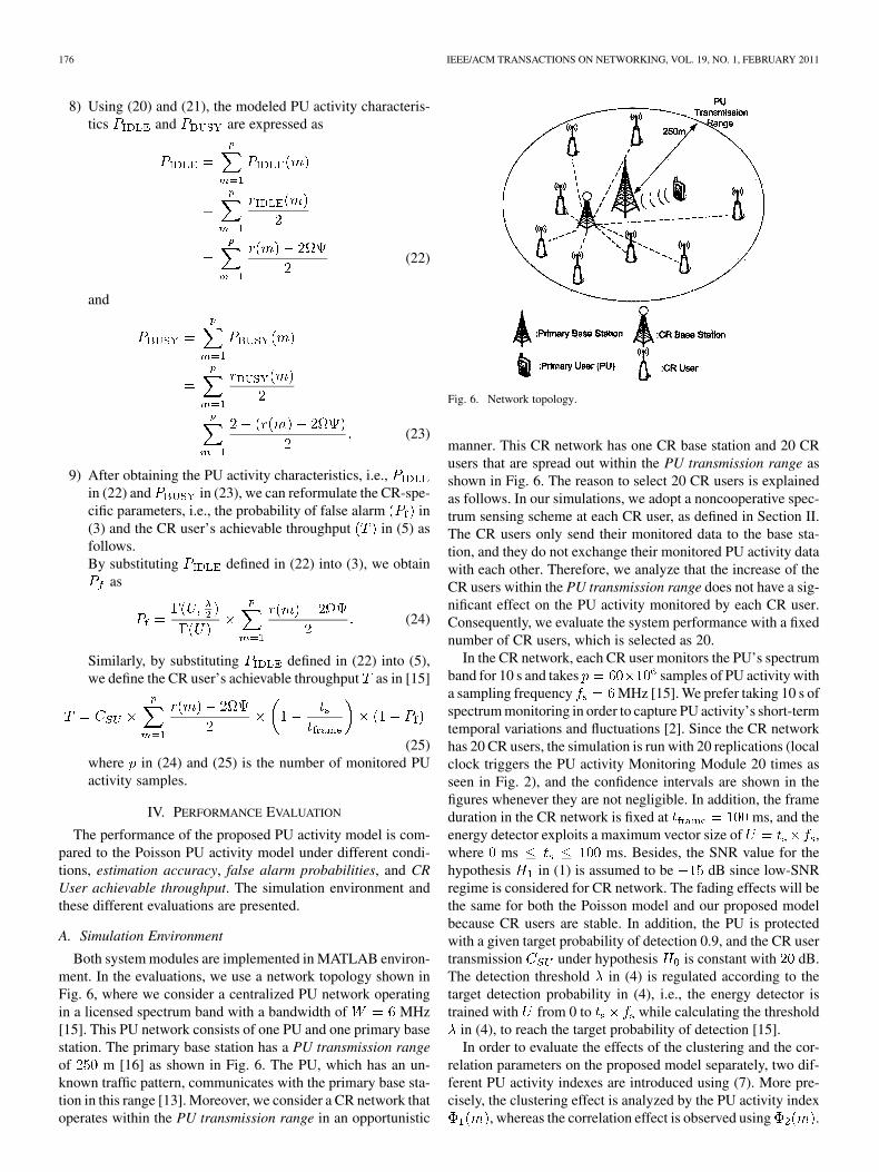
Both system modules are implemented in MATLAB environ-ment. In the evaluations, we use a network topology shown inFig. 6, where we consider a centralized PU network operatingin a licensed spectrum band with a bandwidth of MHz[15]. This PU network consists of one PU and one primary basestation. The primary base station has a PU transmission rangeof m [16] as shown in Fig. 6. The PU, which has an un-known traffic pattern, communicates with the primary base sta-tion in this range [13]. Moreover, we consider a CR network thatoperates within the PU transmission range in an opportunistic

Fig. 6. Network topology.

manner. This CR network has one CR base station and 20 CRusers that are spread out within the PU transmission range asshown in Fig. 6. The reason to select 20 CR users is explainedas follows. In our simulations, we adopt a noncooperative spec-trum sensing scheme at each CR user, as defined in Section II.The CR users only send their monitored data to the base sta-tion, and they do not exchange their monitored PU activity datawith each other. Therefore, we analyze that the increase of theCR users within the PU transmission range does not have a sig-nificant effect on the PU activity monitored by each CR user.Consequently, we evaluate the system performance with a fixednumber of CR users, which is selected as 20.

In the CR network, each CR user monitors the PU’s spectrumband for 10 s and takes samples of PU activity witha sampling frequency MHz [15]. We prefer taking 10 s ofspectrum monitoring in order to capture PU activity’s short-termtemporal variations and fluctuations [2]. Since the CR networkhas 20 CR users, the simulation is run with 20 replications (localclock triggers the PU activity Monitoring Module 20 times asseen in Fig. 2), and the confidence intervals are shown in thefigures whenever they are not negligible. In addition, the frameduration in the CR network is fixed at ms, and theenergy detector exploits a maximum vector size of ,where ms ms. Besides, the SNR value for thehypothesis in (1) is assumed to be dB since low-SNRregime is considered for CR network. The fading effects will bethe same for both the Poisson model and our proposed modelbecause CR users are stable. In addition, the PU is protectedwith a given target probability of detection 0.9, and the CR usertransmission under hypothesis is constant with dB.The detection threshold in (4) is regulated according to thetarget detection probability in (4), i.e., the energy detector istrained with from 0 to while calculating the threshold

in (4), to reach the target probability of detection [15].In order to evaluate the effects of the clustering and the cor-

relation parameters on the proposed model separately, two dif-ferent PU activity indexes are introduced using (7). More pre-cisely, the clustering effect is analyzed by the PU activity index

, whereas the correlation effect is observed using .


and , which are both derived from (7), are ex-plained in detail as follows.

• In the case of the clustering effect , the correlationparameter in (7) is selected by trial as 0.5 for all

. The performance of the proposed modelis evaluated by varying the clustering parameter forall in (7). Thus, (7) becomes

(26)

By substituting (40) into (26), we express asfollows:

(27)

Therefore, the vector is defined using (27) as

(28)

where is the number of monitored PU ac-tivity samples. The reason to select in (7)is explained as follows. 0.5 is the median of the corre-lation values that can take within the range

for all . Therefore, by se-lecting for all , we obtainan equal amount of PU activity samples that pass and failthe -test defined in (44). As seen in (26), which is de-rived from (7), the correlation parameter forall does not have an additional effectto since is kept constant at 0.5 during theevaluations provided by for all .As a result, in (26) only represents the effects ofclustering parameter for all onthe proposed model. In addition, the special case where

for all represents the Poissontraffic model where all samples reside in one cluster.

• In the case of the correlation effect , the clus-tering parameter in (7) is selected as 0.45 for all

because, in the simulations, getsa maximum accuracy at 0.45. Therefore, in (7) iskept fixed at the value 0.45 while varying the correlationparameter for all . Thus, (7)becomes

(29)

By substituting (45) into (29), we express as

(30)

Therefore, the vector is defined using (30) as

(31)

As seen in (29) derived by (7), the clustering parameterfor all does not have an additional

effect to since is kept constant at 0.45 in (7)during the evaluations provided by for all

. Consequently, in (29) only representsthe effects of correlation parameter for all

on the proposed model.In the evaluations, we apply the Min–Max normalization

method [17] on in (27), in (30), and the meansquare error in order to obtain more accurate compar-isons. More precisely, the normalized is denoted as

, and it is calculated using (27) and (28) as

(32)Therefore, the normalized clustering effect is definedusing (32) as

(33)

In the evaluations, we use the notation to represent theelements of the vector in (33). In addition, the special casewhere represents the Poisson traffic model becauseof for all , which indicates thePoisson traffic model where all PU activity samples reside inone cluster.

Similarly, the normalized is denoted as , andit is calculated using (30) and (31) as

(34)Therefore, the normalized correlation effect, , is expressedusing (34) as

(35)

In the evaluations, we use the notation to represent theelements of the vector in (35).

The normalized vector is denoted as , and it isdefined as

(36)

In (36), is the monitored PU activity in (2), and is the mod-eled PU activity calculated using (13). In the evaluations, weuse the notation to represent the elements of the vector

in (36).Overall, we see that in (33) and in (35) are de-

fined using (32) and (34), respectively. Moreover, in(32)) and in (34) are expressed using (26) and (29), re-spectively. Furthermore, (26) and (29) are derived from ,which is calculated in (7). As seen in (8), which is derived from(7), is a function of . Consequently, the equations


Fig. 7. Performance of the proposed model under various �-values. (a) � �

��. (b) � � ��. (c) � � ��. (d) � � ��.

TABLE IVEQUATIONS EVALUATED BY � AND �

that are calculated using can be evaluated by and. More specifically, Table IV summarizes the equations

that are evaluated by and instead of .

B. Overall Performance Comparison for Various -Values

Before giving the detailed results of the evaluations, in thissection, we give an overall performance evaluation of the PUactivity index defined in (8) using Fig. 7. This figure showshow accurate the PU activity model becomes while changingthe . As seen in Fig. 7(a), between 0 and 100 ms, the PUactivity (the solid line) fluctuates around 0 and 8 dBm, andwhen , the PU activity model(the dashed lines) simply approximates all these PU activityfluctuations to a constant value of 5 dBm. Therefore, we canstate that the PU activity model when

cannot accurately estimate the PU activity. How-ever, when increases, i.e., it becomes0.25 [Fig. 7(b)] and 0.45 [Fig. 7(c)], the PU activity model startsestimating the PU activity more accurately. This can be statedbecause when the PU activity fluctuates within 0 and 100 ms,the proposed model fluctuates as well. This leads to more ac-curately capture the spiky characteristics of PU activity. Morespecifically, when , the pro-posed model (the dashed line) fluctuates very accurately when-ever the PU activity (the solid line) fluctuates. When we keepincreasing the , i.e., becomes 0.65 [Fig. 7(d)], the modelstarts to inaccurately estimate the PU activity. Consequently, we

can state that the PU activity model can accurately capture spikyPU activity characteristics when is between 0 and 0.45.

C. Estimation Accuracy

The normalized effects of clustering and correlation on theestimation accuracy are evaluated in two steps. First, we calcu-late and using (16) and (17), respectively. Then,we analyze the normalized mean squared error in (36).

1) Normalized Effects of Clustering and Correlationon and : In Fig. 8(a), we show

and (calculated in (16) and (17), respectively) plottedagainst , which indicates the normalized clustering ef-fect and is calculated by (33). Here, decreases within

and increases within . Weexplain this so-called first-decrease–then-increase phenomenaas follows. When , the number of clusters increasesbecause of the augmentation on the amount of the PU activitysamples that fail the -test given in (37). Since the detectionof PU activity variations is more accurate using clusters, thenumber of periods is increased, leading to a decreasein periods. However, when , there is an in-crease in the number of the PU activity samples that pass inthe -test given in (37). Therefore, the number of clusters de-creases, which leads to a more smooth and burst-free approxi-mation of the PU activity. Consequently, the PU activity fluc-tuations are mistakenly determined, leading to an increase in

periods (or a decrease in periods). Additionally,and [calculated in (16) and (17)] are shown as a

function of the normalized correlation effect [ , calculatedin (35)] in Fig. 8(b), where we observe a direct proportion be-tween and , explained as follows. The rise ofmeans an increase in as seen in (34). Since the increaseof indicates that the correlation parameter is alsoincreased, as observed in (29), the PU activities samples becomesuccessful in the -test given in (44). Therefore, the successfulsamples can reside in the same cluster, leading to an inaccuratedetection of PU activity fluctuations. As a result, this unaware-ness of the PU activities raises the number of IDLE periods (orlowers the number of BUSY periods).

2) Normalized Effects of Clustering and Correla-tion on the : Fig. 9 shows the variations of

[calculated in (36)] in y-axis along [the nor-malized clustering effect that is calculated in (33)] and[the normalized correlation effect that is calculated in (35)] inx-axis. Here, we analyze the first-decrease–then-increase phe-nomena for in the case of , which is described asfollows. Within , the number of clusters in-creases because of the augmentation on the amount of the sam-ples that fail the -test in (37). Since the PU activity fluctuationsare more precisely distinguished using clusters, the proposedmodel achieves more accurate PU activity estimation. More pre-cisely, when , the normalized MSE is 0.62, whereas itbecomes 0.32 when , as shown in Fig. 9. However,within , there is an increase in the number ofthe PU activity samples that are successful in the -test. There-fore, the number of clusters decreases, thereby leading to more


Fig. 8. Normalized clustering effect �� and normalized correlation effect �� on parameters � and � .

Fig. 9. Normalized clustering and correlation effects (� and � ) on�� .

smooth and burst-free identification of the PU activity. Conse-quently, the PU activity fluctuations are inaccurately estimated,i.e., increases within .

In the evaluation provided by the normalized correlation ef-fect , we observe a direct proportion between[calculated in (36)] and [calculated in (35)], as shown inFig. 9. The explanation is as follows. The rise of meansan increase in as seen in (34). The increase of in-dicates that the correlation parameter is also increased,as observed in (29), thereby showing that the correlation levelto be successful in the -test, given in (44) is augmented. Inother words, the PU activity samples are successful in the -testwhen the correlation parameter is increased since they arehighly correlated. Therefore, PU activities samples that are suc-cessful in the -test, given in (44), are accumulated into the samecluster, leading to an inaccurate detection of PU activity fluctu-ations. Consequently, the estimation becomes inaccurate whileraising .

Additionally, the case of gives more accurate MSEestimation than the Poisson model , as seen inFig. 9. More precisely, in the case of , the normalizedMSE is 0.65, whereas for , it is 0.33. This differenceis because of the -values that and have in theevaluations. We see that when , is 1, whereasis 0 for . Therefore, in the case of , thePU activity samples are less successful in the -test than they

Fig. 10. Normalized effects of (a) clustering �� and (b) correlation�� on PU activity parameters � and � .

are in the case of , because of is lower thanof . Consequently, less PU activity samples can be ac-

cumulated into the same cluster when compared to, leading to more accurate detection of PU activity.

D. False-Alarm Probability

The normalized effects of clustering and correlationon the false-alarm probability are evaluated in two

steps. First, we calculate the PU activity characteristicsand using (22) and (23), respectively. Then, we analyzethe in (24) using .

1) Normalized Effects of Clustering and Correla-tion on and : In Fig. 10(a) and (b), weshow the variations of the PU activity characteristics in y-axisalong the normalized effects of clustering [ , calculated in(33)] and correlation [ , calculated in (35)] in x-axis, re-spectively. Recall that the PU activity characteristics and

are obtained by and using (22) and (23),respectively.

and are inversely proportional since. More specifically, in Fig. 10(a), we

observe the first-decrease–then-increase phenomenon forand the first-increase–then-decrease phenomenon for. The explanation of these two opposite phenomena is


Fig. 11. Normalized effects of clustering �� and correlation �� onthe false-alarm probability � .

as follows. Within , the number of clusters,created by the PU activity samples, increases because of theincrease in the amount of the samples that failed the -test in(44). Since the detection of PU activity fluctuations becomesmore accurate using clusters, the number of captured BUSYperiods is increased (or the number of IDLE periods is de-creased), leading to an increase in (or to a decreasein ). However, within , the numberof the PU activity samples that are successful in the -test, isincreased, thereby decreasing the number of clusters, whichleads to more smooth and burst-free approximation of thePU activity. Consequently, the spiky characteristics of the PUactivity are mistakenly determined, leading to an increase in

(or to an decrease in ). In the case of asshown in Fig. 10(b), we observe a direct proportion between

and (and an inverse proportion betweenand ). The rise of means an increase in asseen in (34). Since the increase of indicates that thecorrelation parameter is also increased, as observedin (29), PU activities samples become successful in the -testgiven in (44). Therefore, they can reside in the same clusterleading to an inaccurate detection of PU activity fluctuations.As a result, increases (or decreases) because ofthe unawareness of the PU activities, as long as increases.

2) Normalized Effects of Clustering and Correlationon : The normalized effects of clustering

and correlation on the false-alarm probability areobtained by (24) and demonstrated in Fig. 11, where thein y-axis is plotted as functions of [calculated in (33)]and [calculated in (35)] in x-axis. As shown in Fig. 11,

presents the first-decrease–then-increase phenomena in thecase of . When , the number of clusters in-creases because of the increase in the number of the samplesthat fail the -test, given in (37). Since the PU activity fluc-tuations are more accurately identified using clusters,is decreased, which leads to a decrease in the in (24). Asa result, the is 0.6 when , whereas it becomes0.38 when , as shown in Fig. 11. However, when

, there is an augmentation in the number of the PUactivity samples that are successful in the -test. Therefore, thenumber of clusters decreases, which leads to more smooth andburst-free characterization of the PU activity. Consequently, thePU activity fluctuations are inaccurately estimated. Moreover,

is directly proportional to , as shown in Fig. 11. Sincethe rise of means an increase in the correlation parameter

, as we observe in (29), PU activity samples are successfulin the -test, given in (44), hence they can be accumulated intothe same cluster. Therefore, increases because of the un-awareness of the PU activities, leading to an increase of in(24). However, in the case of , our proposed modelprovides , which is 25% less than the provided byPoisson model , which is 0.67, as seen in Fig. 11.

E. CR User Achievable Throughput

The performance of the proposed model is also evaluated interms of the CR user’s achievable throughput. Fig. 12(a) and(b) represent the CR user’s throughput [calculated in (25)] asfunctions of the [given in (33)] and [given in (35)],respectively.

In Fig. 12(a), within , we observe anincrease in the throughput from to b/s/Hz. The reasonfor this increase is expressed as follows. As ,the number of PU samples that fail the -test given in (37)also increases, thereby raising the number of clusters. Sincethe PU activity fluctuations are more accurately capturedusing clusters, there is a reduction of , which is calculatedin (24). Therefore, the last term in (25) increases,which leads to an augmentation in throughput. However, within

, the last term in (25) decreases due tothe higher , caused by the inaccurate PU activity detection,thereby degrading the throughput from to b/s/Hz. Inthe case of , we observe a continuous reduction in theCR user’s throughput as shown in Fig. 12(b). Sinceand are directly proportional as demonstrated in Fig. 11,the last term in (25) decreases continuously while increasing

, which results in throughput degradation. Although thethroughput decreases with , in the case of , ourproposed model provides a throughput of b/s/Hz, whichis 26% higher than the one provided by the Poisson model

, which is b/s/Hz, as seen in Fig. 12(b).Overall, the key results are summarized in Table V, where

the proposed model outperforms the Poisson model, giving sig-nificant improvements in the normalized PU activity estima-tion error , the false-alarm probability , and CR user’sthroughput .

V. CONCLUSION

In this paper, a novel PU activity model based on the first-dif-ference filter clustering and enhanced with temporal correlationstatistics is introduced. The scheme, which has the capability ofclustering and modeling the PU activity fluctuations, addressesthe potential drawbacks of Poisson model in the sense of moreaccurate PU detection and more effective usage of transmissionopportunities. The proposed model is evaluated by simulationsusing the normalized clustering and correlationeffects. The comprehensive performance evaluation shows thatthe model gives more accurate estimation, less false-alarmprobabilities, and higher throughput than the Poisson modelingwithin an interval of and for .It is planned to apply the proposed PU activity model intoexperimental scenarios by employing a test bed, where CR


Fig. 12. Normalized effect of clustering �� and correlation �� on achievable throughput � .

TABLE VKEY RESULTS

users are mobile and adopt the cooperative spectrum sensing.Moreover, the PU mobility issues will be added to the model,and the performance of and will be evaluated.

APPENDIX ACLUSTERING PARAMETER AND -TEST

The clustering parameter is a value to form clusters usingthe first-difference filtering procedure called -test, which is re-alized as follows:

otherwise(37)

where is the th sample of , which is the modeled PUactivity vector; is the cluster index with , and isthe th output of the first-difference FIR filter with input .

is defined as

(38)

Using and , the first-difference outputof the filter becomes

(39)

We may assume that the modeled PU activity vector is iden-tical to the monitored PU activity vector in the Clustering-Modeling Module. However, at the output of the Clustering-Modeling Module, the new modeled PU vector will be formed,thus is not identical to the monitored PU activity vector . In

(37), represents the th clustering parameter to be usedfor the -test. The output of the hypothesis test defined in (37) isinterpreted as successful if , whereas the outputis interpreted as fail if otherwise. More specifically, assuming

is a sample of the cluster , the test indicates thatand belong to the same cluster if the difference

of the power levels between and is below .In this case, the -test defined in (37) is successful. On the otherhand, the test is fail if the difference between the powers ofand exceeds , which shows that they are not lo-cated within the same cluster. Besides, in cases where the testresults in fail, a new cluster is generated, andbecomes the first sample of the .

The -test explained is directly affected by the variations of. Furthermore, the overall performance of the system in

terms of PU activity detection is also influenced. This effect isexplained as follows. When , meaning thatin (37), it implies that the -test is successful as long as

. This indicates that each modeled PU activity sample islocated in a different cluster unless the sample is identical to itspredecessor. In such cases, since the number of the modeled PUactivity samples in a cluster is one, the Clustering Engine func-tion is bypassed. Moreover, if is selected as ,-test in (37) is successful for most of the modeled PU activity

samples since the difference between any two consecutive sam-ples’ power levels is lower than . Therefore, all modeledPU activity samples residing in one cluster imply that the PU ac-tivity is becoming smooth. Consequently, when we accumulatethe PU activity samples into clusters, we exploit the similaritiesand correlations within these samples.

As explained, the -test in (37) indicates that the output ofthe first-difference filter in (39) is directly affected bythe cluster parameter . Hence, using (39), we approximate

as follows:

(40)

where shows the effect of the clustering parameter on themodeled PU activity sample . Consequently, a vector ofclustering parameters is generated using (40) as follows:

(41)


In the evaluations, we use the notation to represent the ele-ments of the vector in (41).

APPENDIX BCORRELATION PARAMETER, -TEST, AND CORRELATION SLOPE

The correlation parameter is a value that indicates thetemporal correlation level that the consecutive PU activity sam-ples need to achieve to reside in the same cluster. This correla-tion level is calculated by the Linear Pearson Product-MomentCorrelation,1 , [18] which is expressed as

(42)

where represents the sample index vector, is the mod-eled PU activity sample vector, is the mean, and is thestandard deviation. By substituting in (42), we calculatethe correlation level for the last three PU activity samples by

(43)

where , and is a subvector that has the lastthree samples of the modeled PU activity , expressed as

Consequently, a correlation calculation procedure called-test is realized using 43 as follows:

otherwise(44)

where represents the correlation parameter to be usedfor the -est of the th modeled PU activity sample . Thereason to take the last three values is as follows. It is empiricallyfound that taking the last three samples will give sufficient infor-mation about the correlation level of the monitored PU activityvector. Since we use a linear correlation, taking two samples willnot give us a precise idea to decide whether is correlatedwith its predecessors or not. If we take more than three samplesfor the linear correlation, we observed that the correlation levelcannot accurately capture the spiky characteristics of the sam-ples. Therefore, we use an optimum value of three samples totake for correlation calculations. In addition, the absolute valueof is preferred because the proposed system fo-cuses on the amount of correlation and its slope separately.

The output of the hypothesis test in (44) is interpreted as suc-cessful if , and as fail if otherwise.More precisely, the test is successful when the correlation level

1� indicates the notation of a vector � with � elements

within the last three consecutive samples of the modeled PU ac-tivity exceeds . Therefore, we state that these three sam-ples are highly correlated, hence they have similar characteris-tics. On the contrary, the last three samples are not highly corre-lated as long as the correlation level is below . Moreover,in both cases, we observe by trial that the correlation level cal-culated in (43) used in this test is directly affected by .Then, we map the correlation level, calculated in (43), to thecorrelation parameter and express as follows:

(45)

where is the total number of PU monitored activity samples.Accordingly, a vector of correlation parameters is gener-ated as follows:

(46)

In the evaluations, we use the notation to represent the ele-ments of the vector in (46).

The -test in (44) is applied in the Clustering Engine to in-dicate the correlation level for the modeled PU activity sam-ples in order to be located within a cluster. Moreover, the useof the -test in the Clustering Engine can be interpreted as across-check; i.e., even though the -test defined in (37) is passed,if the modeled PU activity samples are not highly correlated,they are prohibited to be in the same cluster. This is importantbecause when the number of modeled PU activity samples ina cluster increases, some of them can be less correlated. As aresult, this cross-check avoids such misleading results and putsuncorrelated samples in different clusters.

The -test is also utilized in the Modeling Engine, as given inFig. 2, to decide whether the last three clusters, ,

and with cluster index , are highly correlated or not.Recall that any th cluster is represented by . Accordingly,the -test in the Modeling Engine is defined as

(47)

In (47), is calculated by substituting andin (42) as

(48)

where is the triple of clusters defined as

(49)


The correlation slope test that is realized in the Modeling En-gine in Fig. 2 is defined as

(50)

where is defined by substituting andin (42) as

(51)

In (51), is the pair of clusters defined asand . The correlation

slope test defined in (50) is used in order to indicate that con-secutive clusters and show similar or oppositelinear trend. More specifically, the slope of ispositive, if and are in an increasing linear rela-tionship that also indicates that . Furthermore,the slope becomes negative if they are in a decreasing linearrelationship that shows that .

ACKNOWLEDGMENT

The authors would like to thank X. Gelabert, K. Chowdhury,W.-Y. Lee, as well as the Editor, Milind Buddhikot, and thereviewers for their constructive feedbacks.

REFERENCES

[1] I. F. Akyildiz, W.-Y. Lee, M. C. Vuran, and S. Mohanty, “Next gen-eration/dynamic spectrum access/cognitive radio wireless networks: Asurvey,” Comput. Netw., vol. 50, no. 13, pp. 2127–2159, Sep. 2006.

[2] D. Willkomm, S. Machiraju, J. Bolot, and A. Wolisz, “Primary usersin cellular networks: A large-scale measurement study,” in Proc. 3rdIEEE DySPAN, Oct. 2008, pp. 1–11.

[3] W.-Y. Lee and I. F. Akyildiz, “Optimal spectrum sensing frameworkfor cognitive radio networks,” IEEE Trans. Wireless Commun., vol. 7,no. 10, pp. 3845–3857, Oct. 2008.

[4] Y. Chen, Q. Zhao, and A. Swami, “Joint design and separation principlefor opportunistic spectrum access in the presence of sensing errors,”IEEE Trans. Inf. Theory, vol. 54, no. 5, pp. 2053–2071, May 2007.

[5] A. A. Daoud, M. Alanyali, and D. Starobinski, “Secondary pricing ofspectrum in cellular CDMA networks,” in Proc. 2nd IEEE DySPAN,Apr. 2007, pp. 535–542.

[6] C.-T. Chou, N. S. Shankar, H. Kim, and K. Shin, “What and how muchto gain by spectrum agility?,” IEEE J. Sel. Areas Commun., vol. 25, no.3, pp. 576–588, Apr. 2007.

[7] V. Paxson and S. Floyd, “Wide-area traffic: The failure of Poisson mod-eling,” IEEE/ACM Trans. Netw., vol. 3, no. 3, pp. 226–244, Jun. 1995.

[8] R. Jain, S. Shawn, and A. Routhier, “Packet trains: Measurements and anew model for computer network traffic,” IEEE J. Sel. Areas Commun.,vol. SAC-4, no. 6, pp. 986–995, Sep. 1986.

[9] T. Renk, C. Kloeck, F. K. Jondral, P. Cordier, O. Holland, and F.Negredo, “Spectrum measurements supporting reconfiguration in het-erogeneous networks,” in Proc. 16th IST Mobile Wireless Commun.Summit, Jul. 2007, pp. 1–5.

[10] T. Kamakaris, M. M. Buddhikot, and R. Iyer, “A case for coordinateddynamic spectrum access in cellular networks,” in Proc. 1st IEEEDySPAN, Nov. 2005, pp. 289–298.

[11] J. Guo, F. Liu, and Z. Zhu, “Estimate the call duration distribution pa-rameters in GSM system based on K-L divergence method,” in Proc.WiCom, 2007, pp. 2988–2991.

[12] J. Ma and Y. Li, “A probability-based spectrum sensing scheme forcognitive radio,” in Proc. IEEE ICC, May 2008, pp. 3416–3420.

[13] F. F. Digham, M.-S. Alouini, and M. K. Simon, “On the energy detec-tion of unknown signals over fading channels,” IEEE Trans. Commun.,vol. 55, no. 1, pp. 21–24, Jan. 2007.

[14] H. Tang, “Some physical layer issues of wide-band cognitive radio sys-tems,” in Proc. 1st IEEE DySPAN, Nov. 2005, pp. 151–159.

[15] Y.-C. Liang, Y. Zeng, E. Peh, and A. T. Hoang, “Sensing-throughputtradeoff for cognitive radio networks,” IEEE Trans. Wireless Commun.,vol. 7, no. 4, pp. 1326–1337, Apr. 2008.

[16] Z. Guomei, I. F. Akyildiz, and G. S. Kuo, “STOD-RP: A spectrum-tree based on-demand routing protocol for multi-hop cognitive radionetwork,” in Proc. IEEE GLOBECOM, Dec. 2008, pp. 1–5.

[17] J. Hann and M. Kamber, Data Mining: Concepts and Techniques.San Mateo, CA: Morgan Kaufman, 2000.

[18] J. L. Rodgers and A. W. Nicewander, “Thirteen ways to look at thecorrelation coefficient,” Amer. Statistician, vol. 42, no. 1, pp. 59–66,1988.

Berk Canberk (S’10) received the B.Sc. degreein electrical engineering from Istanbul TechnicalUniversity, Istanbul, Turkey, in 2003, and theM.Sc. degree in digital communication engineeringfrom the Department of Computer Science andEngineering, Chalmers University of Technology,Göteborg, Sweden, in 2005. He is currently pur-suing the Ph.D. degree in the Computer NetworksResearch Laboratory of the Computer EngineeringDepartment, Istanbul Technical University.

He was a Visiting Scholar with the BroadbandWireless Networking Laboratory, School of Electrical and Computer Engi-neering, Georgia Institute of Technology, Atlanta, from 2008 to 2009. Hiscurrent research interest is the spectrum modeling and management in cognitiveradio networks.

Ian F. Akyildiz (M’86–SM’89–F’96) received theB.S., M.S., and Ph.D. degrees in computer engi-neering from the University of Erlangen-Nurnberg,Germany, in 1978, 1981, and 1984, respectively.

Currently, he is the Ken Byers Distinguished ChairProfessor with the School of Electrical and ComputerEngineering, Georgia Institute of Technology, At-lanta, as well as the Director of Broadband WirelessNetworking Laboratory and Chair of the Telecom-munication Group at Georgia Tech. In June 2008, hebecame an Honorary Professor with the School of

Electrical Engineering, Universitat Politecnica de Catalunya (UPC), Barcelona,Spain. He is also the Director of the newly founded N3Cat (NaNoNetworkingCenter in Catalunya). He is the Editor-in-Chief of Computer Networks andthe founding Editor-in-Chief of the journals Ad Hoc Networks and PhysicalCommunication. He serves on the advisory boards of several research centers,journals, conferences, and publication companies. His research interests are innanonetworks, cognitive radio networks, and wireless sensor networks.

Dr. Akyildiz has been a Fellow of the Association for Computing Machinery(ACM) since 1997. He has received numerous awards from the IEEE and ACM.

Sema Oktug (M’91) received the B.Sc., M.Sc.,and Ph.D. degrees in computer engineering fromBogazici University, Istanbul, Turkey, in 1987, 1989,and 1996, respectively.

Currently, she is a Professor with the Departmentof Computer Engineering, Istanbul Technical Univer-sity, Istanbul, Turkey. She is the coordinator of theComputer Networks Research Laboratory in the De-partment of Computer Engineering. She also servesas Vice-Dean of the Faculty of Electrical ElectronicsEngineering, Istanbul Technical University. She is on

the Editorial Board of Computer Networks. Her research interests are in commu-nication protocols, modeling and analysis of communication networks, wirelessnetworks, and optical WDM networks.

Date post:	18-Dec-2016
Category:	Documents
Upload:	sema
View:	212 times
Download:	0 times

Primary User Activity Modeling Using First-Difference Filter Clustering and Correlation in Cognitive...

Documents