Page 1
Probabilistic Failure Analysis of Complex Systems with Case
Studies in Nuclear and Hydropower Industries
by
Ahmed El-Awady
A Thesis
presented to the University of Waterloo
in fulfillment of the
thesis requirement for the degree of
Doctor of Philosophy
in
Systems Design Engineering
Waterloo, Ontario, Canada, 2019
© Ahmed El-Awady 2019
Page 2
ii
Examining Committee Membership
The following served on the Examining Committee for this thesis. The decision of the
Examining Committee is by majority vote.
External Examiner NAME: Slobodan P. Simonović
Title: Professor, Civil and Environmental Engineering, The
University of Western Ontario
Supervisor NAME: Kumaraswamy Ponnambalam
Title: Professor, Systems Design Engineering, University of
Waterloo
Internal Member NAME: Keith W. Hipel
Title: Professor, Systems Design Engineering, University of
Waterloo
Internal Member NAME: Shi Cao
Title: Assistant Professor, Systems Design Engineering,
University of Waterloo
Internal-external Member NAME: Bryan Tolson
Title: Associate Professor, Civil and Environmental
Engineering, University of Waterloo
Page 3
iii
Author’s Declaration
This thesis consists of material all of which I authored or co-authored: see Statement of
Contributions included in the thesis. This is a true copy of the thesis, including any required final
revisions, as accepted by my examiners.
I understand that my thesis may be made electronically available to the public.
Page 4
iv
Statement of Contributions
1- Ponnambalam, K.; El-Awady, A.; Mousavi, S. J. & Seifi, A. 2019. “Simulation
Supported Bayesian Network for Estimating Failure Probabilities of Dams,” in ICOLD
87th
annual meeting and symposium, June 2019, Ottawa, Canada. (Accepted Paper)
2- El-Awady, A.; Ponnambalam, K.; Bennett, T.; Zielinski, A. & Verzobio, A. 2019.
“Bayesian Network Approach for Failure Prediction of Mountain Chute Dam and
Generating Station,” in ICOLD 87th
annual meeting and symposium, June 2019, Ottawa,
Canada. (Accepted Paper)
3- El-Awady, A. & Ponnambalam, K. 2019. “A Decomposition Approach Using Bayesian
Networks and Markov Chains for Probabilistic Failure Analysis of Dams,” in the
8th
International Conference on Water Resources and Environment Research (ICWRER),
June 2019, Hohai University, Nanjing, China. (Accepted Extended Abstract)
4- Verzobio, A.; El-Awady, A.; Ponnambalam, K.; Quigley, J. & Zonta, D. 2019.
“Elicitation Process to Populate Bayesian Networks with Application to Dams Safety,” in
the 8th
International Conference on Water Resources and Environment Research
(ICWRER), June 2019, Hohai University, Nanjing, China. (Accepted Extended
Abstract)
5- El-Awady, A. & Ponnambalam, K. 2019. “Bayesian Network (BN) Approach for Failure
Prediction of Deep Geological Nuclear Waste Repository,” in CNS Conference on
Nuclear Waste Management, Decommissioning, and Environmental Restoration
(NWMDER), September 2019, Ottawa, Canada. (Accepted Abstract, Paper Submitted,
Approval Pending)
Page 5
v
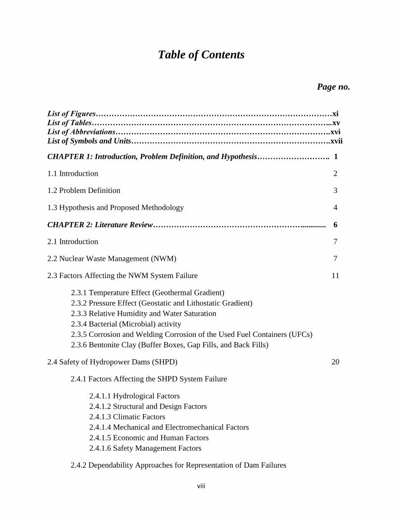
Abstract
Detailed Monte-Carlo simulation of a complex system is the benchmark method used in probabilistic analysis
of engineering systems under multiple uncertain sources of failure modes; such simulations typically involve a
large amount of CPU time. This makes the probabilistic failure analysis of complex systems, having a large
number of components and highly nonlinear interrelationships, computationally intractable and challenging.
The objective of this thesis is to synthesize existing methods to analyze multifactorial failure of complex
systems which includes predicting the probability of the systems failure and finding its main causes under
different situations/scenarios. Bayesian Networks (BNs) have potentials in probabilistically representing
complex systems, which is beneficial to predicting the systems failure probability and diagnosing its causes
using limited data, logic inference, expert knowledge or simulation of system operations. Compared to other
graphical representation techniques such as Event Tree Analysis (ETA) and Fault Tree Analysis (FTA), BNs
can deal with complex networks that have multiple initiating events and different types of variables in one
graphical representation with the ability to predict the effects, or diagnose the causes leading to a certain
effect. This thesis proposes a multifactor failure analysis of complex systems using a number of BN-based
approaches. In order to overcome limitations of traditional BNs in dealing with computationally intensive
systems simulation and the systems having cyclic interrelationships (or feedbacks) among components,
Simulation Supported Bayesian Networks (SSBNs) and Markov Chain Simulation Supported Bayesian
Networks (MCSSBNs) are respectively proposed. In the latter, Markov Chains and BNs are integrated to
acquire analysis for systems with cyclic behavior when needed. Both SSBNs and MCSSBNs have the
distinction of decomposing a complex system to many sub-systems, which makes the system easier to
understand and faster to be simulated. The efficiency of these techniques is demonstrated first through their
application to a pilot system of two dam reservoirs, where the results of SSBNs and MCSSBNs are compared
with those of the entire system operations simulation. Subsequently, two real-world problems including failure
analysis of hydropower dams and nuclear waste systems are studied. For such complex networks, a bag of
tools that depend on logically inferred data and expert knowledge and judgement are proposed for efficiently
predicting failure probabilities in cases where limited operational and historical data are available. Results
demonstrate that using the proposed SSBN method for estimating the failure probability of a two dam
reservoir system of different connections/topologies results in probability estimates in the range of 3%, which
are close to those coming from detailed simulation for the same system. Increasing the number of states per
BN variables in the states’ discretization stage makes the SSBN results converge to the simulation results.
When Markov chains are integrated with SSBN (i.e. MCSSBN), the results depend on the MCSSBN approach
that is used according to the scenarios of interest that need to be included in the BN representation. Evidence
of system failure can be used to diagnose the main contributors to the failure (i.e. inflow, reservoir level, or
defected gates). This posterior diagnostic capability of the BN is distinctive for the real world case studies
presented in this thesis. In Mountain Chute Dam that is operated by Ontario Power Generation, the main
contributors to system failure, according to the logically inferred data and expert knowledge, are inadequate
discharge capacity of the sluiceway, electromechanical equipment failure, head gates failure, non-safe ice
loading, high inflow, high rain/precipitation, sluice gate failure, and high water pressure. While for the
Nuclear Waste Management system, the main contributors to system failure according to the known and
assumed data are due to high pressures and bentonite failures. In summary, modelling, validating, and
developing appropriate modifications of the BN method for applications in complex systems failure analysis is
the major contribution of this thesis.
Page 6
vi
Acknowledgement
Firstly, I would like to thank my God; ALLAH; for his graces and gifts.
EGYPT, my home country, I hope to be one of the contributors in creating your better future.
I would like to express my special appreciation and thanks to my supervisor Prof. Kumaraswamy
Ponnambalam (Ponnu), you have been a tremendous mentor for me. I would like to thank you for
encouraging my research and for allowing me to grow as a research scientist. Your seamless
support, advice, and guidance have been priceless.
I would also like to thank my committee members, Prof. Keith W. Hipel, Prof. Shi Cao, and Prof.
Bryan Tolson for serving as my committee members. Special thanks to Prof. Slobodan P.
Simonovic for being my external examiner. I also want to thank you for letting my defense be an
enjoyable moment, and for your brilliant comments and suggestions, thanks to you.
I would especially like to thank Prof. Alcigeimes B. Celeste (Geimes), and Prof. S. Jamshid
Mousavi for their academic guidance during their visiting professorship at the University of
Waterloo.
Many thanks to my research team mates, Dr. Jorge A. Garcia, Shankai Lin, Vimala
Madhusoothanan, and Mythreyi Sivaraman, for sharing me their thoughts and data for the NWM
case study.
I really appreciate the effort that Andrea Verzobio, International Visiting Graduate Student at
UWaterloo during Fall 2018, spent with me in getting some valuable results for the case study of
Mountain Chute Dam.
Special thanks to both, Ontario Power Generation (OPG), and Nuclear Waste Management
Organization (NWMO), and their executives, for their support.
A special thanks to my father and mother, father-in-law and mother-in-law. Words cannot
express how grateful I am to you for all of the sacrifices that you’ve made on my behalf.
My precious and dear wife, Reham, you have always been my support in the moments when there
was no one to answer my queries. Thank you for your patience, and for taking care of our
beloved kids: Basel, Jasmine, and Tarek.
Page 7
vii
Dedication
To
The inspirational soul of my Grandfather, sorry for not completing this work before you can see it,
TAREK; my supportive DAD,
HANAA; my bright MOM,
REHAM; my lovely WIFE,
My beloved kids; BASEL, JASMINE, and TAREK Jr.,
And my godfather; Prof. MOHSEN…….
Page 8
viii
Table of Contents
Page no.
List of Figures………………………………………………………………………………xi
List of Tables………………………………………………………………………………..xv
List of Abbreviations……………………………………………………………………….xvi
List of Symbols and Units………………………………………………………………….xvii
CHAPTER 1: Introduction, Problem Definition, and Hypothesis………………………. 1
1.1 Introduction 2
1.2 Problem Definition 3
1.3 Hypothesis and Proposed Methodology 4
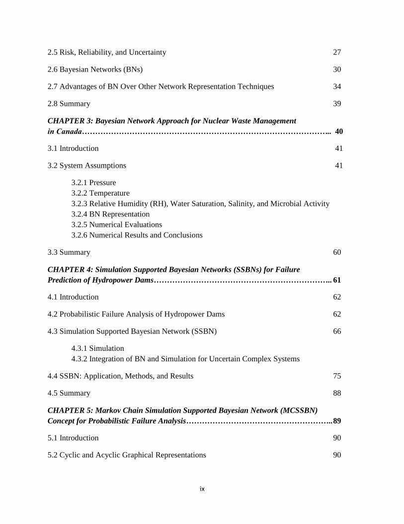
CHAPTER 2: Literature Review…………………………………………………............ 6
2.1 Introduction 7
2.2 Nuclear Waste Management (NWM) 7
2.3 Factors Affecting the NWM System Failure 11
2.3.1 Temperature Effect (Geothermal Gradient)
2.3.2 Pressure Effect (Geostatic and Lithostatic Gradient)
2.3.3 Relative Humidity and Water Saturation
2.3.4 Bacterial (Microbial) activity
2.3.5 Corrosion and Welding Corrosion of the Used Fuel Containers (UFCs)
2.3.6 Bentonite Clay (Buffer Boxes, Gap Fills, and Back Fills)
2.4 Safety of Hydropower Dams (SHPD) 20
2.4.1 Factors Affecting the SHPD System Failure
2.4.1.1 Hydrological Factors
2.4.1.2 Structural and Design Factors
2.4.1.3 Climatic Factors
2.4.1.4 Mechanical and Electromechanical Factors
2.4.1.5 Economic and Human Factors
2.4.1.6 Safety Management Factors
2.4.2 Dependability Approaches for Representation of Dam Failures
Page 9
ix
2.5 Risk, Reliability, and Uncertainty 27
2.6 Bayesian Networks (BNs) 30
2.7 Advantages of BN Over Other Network Representation Techniques 34
2.8 Summary 39
CHAPTER 3: Bayesian Network Approach for Nuclear Waste Management
in Canada………………………………………………………………………………….. 40
3.1 Introduction 41
3.2 System Assumptions 41
3.2.1 Pressure
3.2.2 Temperature
3.2.3 Relative Humidity (RH), Water Saturation, Salinity, and Microbial Activity
3.2.4 BN Representation
3.2.5 Numerical Evaluations
3.2.6 Numerical Results and Conclusions
3.3 Summary 60
CHAPTER 4: Simulation Supported Bayesian Networks (SSBNs) for Failure
Prediction of Hydropower Dams………………………………………………………….. 61
4.1 Introduction 62
4.2 Probabilistic Failure Analysis of Hydropower Dams 62
4.3 Simulation Supported Bayesian Network (SSBN) 66
4.3.1 Simulation
4.3.2 Integration of BN and Simulation for Uncertain Complex Systems
4.4 SSBN: Application, Methods, and Results 75
4.5 Summary 88
CHAPTER 5: Markov Chain Simulation Supported Bayesian Network (MCSSBN)
Concept for Probabilistic Failure Analysis……………………………………………….. 89
5.1 Introduction 90
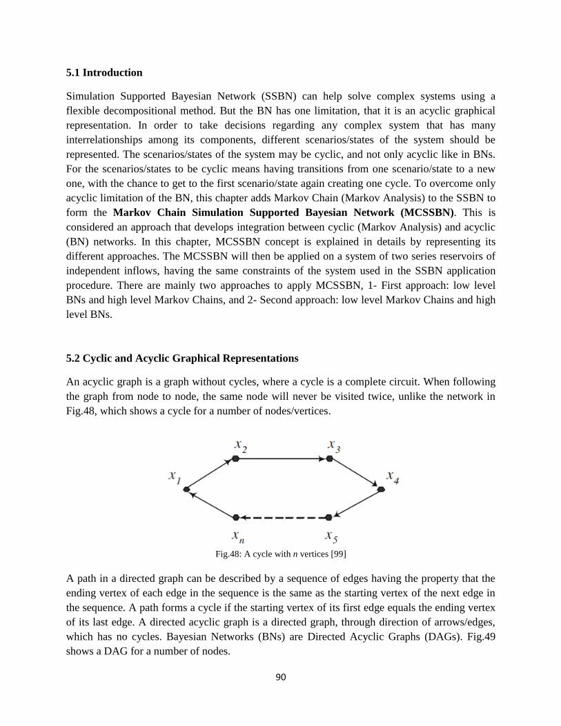
5.2 Cyclic and Acyclic Graphical Representations 90
Page 10
x
5.3 Markov Chain Analysis 91
5.4 Markov Chain Simulation Supported Bayesian Network (MCSSBN) 93
5.4.1 First Approach of MCSSBN
5.4.2 Second Approach of MCSSBN
5.5 Methods of Applying MCSSBN to a System of Three Dam Reservoirs 103
5.5.1 MCSSBN First Approach
5.5.2 MCSSBN Second Approach
5.6 MCSSBN First Approach for Two Series Reservoirs 108
5.7 MCSSBN Second Approach for Two Series Reservoirs 117
5.8 Summary 127
CHAPTER 6: A Real-World Case Study: Mountain Chute Dam……………………….. 129
6.1 Introduction 130
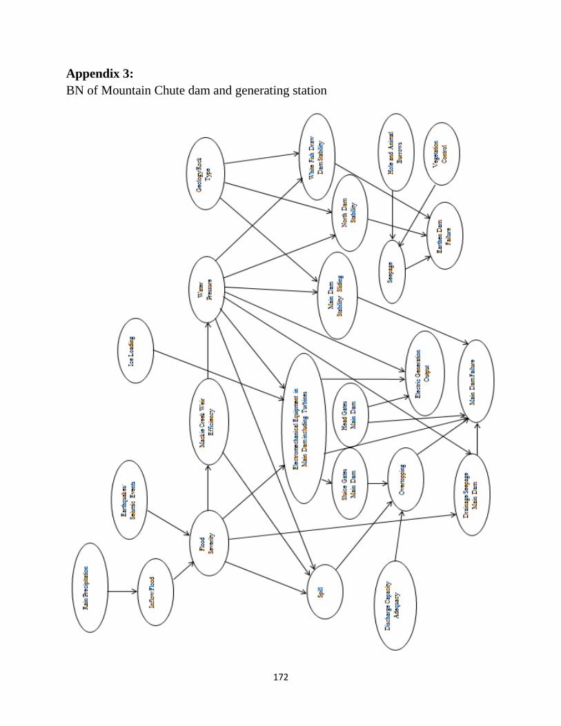
6.2 BN of Mountain Chute 130
6.3 Quantifying the BN Using Available Data and Logic Inference 133
6.3.1 BN Input Data and Results
6.4 Expert Judgement for Quantifying the BN of Mountain Chute Dam 143
6.5 Summary, Comments, and Recommendations 151
CHAPTER 7: Conclusions, Recommendations, and Future Work……………………… 153
7.1 Conclusions 154
7.2 Recommendations 155
7.3 Limitations 156
7.4 Future Work 157
References……...………………………………………………………………………...... 158
Appendices…………………………………………………………………………………. 166
Appendix 1
Appendix 2
Appendix 3
Page 11
xi
List of Figures
Figure Page no.
Fig.1: Final Disposal Facility for spent nuclear fuel (High Level Waste HLW) [14]……... 9
Fig.2: ACR-1000 FUEL Bundle (~ 20 kg) [16]…………………………………………… 10
Fig.3: The conceptual container design for the disposal of Canadian high level
nuclear waste [12]……………………………………………………………….... 11
Fig.4: Schematic representation of the proposed Canadian Deep Geological
Repository (DGR) [12]………………………………………………………….... 11
Fig.5: Geological Regions of Canada [28]……………………………………………….... 14
Fig.6: Spent fuel container and its coating [33]…………………………………………… 18
Fig.7: Bentonite Buffer box [33]…………………………………………………………... 19
Fig.8: Placement Room Concept [33]…………………………………………………....... 19
Fig.9: Placement Room (side view)……………………………………………………….. 20
Fig.10: Progressive headcutting breach of a cohesive soil embankment [43]…………….. 22
Fig.11: An example of FTA with different dam failure modes [60]……...……………….. 27
Fig.12: Risk management process [64]……………………………………………………. 28
Fig.13: Types of reasoning in BNs [77]…………………………………………………… 31
Fig.14: An example of BN with seven variables [78]…………………………………....... 32
Fig.15: Bayesian network of earthquake-triggered landslides [79]………………………... 32
Fig.16: The BN structure of the IEEE-RTS system [83]………………………………...... 34
Fig.17: BN of two series dependent dams/reservoirs…………………………………....... 37
Fig.18: BN of two parallel dependent dams/reservoirs……………………………………. 37
Fig.19: ETA of two dependent dams/reservoirs………………………………………....... 38
Fig.20: Used Fuel Container Manufacturing Process [85]……………………………........ 42
Fig.21: Copper Coated Used Fuel Container [85]………………………………………… 43
Fig.22: Underground Repository Layout [85]…………………………………………….. 43
Fig.23: Placement Room Geometry (Vertical Section) [85]………………………………. 44
Fig.24: Current Nuclear Fuel Waste Major Storage Locations in Canada [86]…………… 44
Fig.25: Probability of having active SRB as a function of dry density…………………… 48
Fig.26: Proposed BN of NWM systems…………………..……………………………… 50
Fig.27: BN determining the main factors contributing in a failure, given a
failure took place…………………………………………………………………. 58
Fig.28: Posterior probability of failure given the evidence of pressure less than
45 MPa and high density bentonite……………………………………………… 59
Fig.29: Example of a Dam System Model [88]…………………………………………… 63
Fig.30: Variables involved in diagnosing distresses associated with overtopping
of dams [7]……………………………………………………………………….. 64
Page 12
xii
Fig.31: Causal network for diagnosing distresses associated with seepage
erosion–piping of dams [7]………………………………………………………. 64
Fig.32: Probability calculation for diagnosing distresses of dams using Hugin
Lite program [7]………………………………………………………………….. 65
Fig.33: Dynamic Bayesian network for predicting water availability in a
water distribution network [96]…………………………………………………... 67
Fig.34: Proposed Methodology of SSBN…………………………………………………. 68
Fig.35a: A 23 node BN using Hugin software……………………………………………. 69
Fig.35b: A 23 node BN decomposed to 6 sub-entities ready to be simulated…………….. 70
Fig.36: Bayes-Markov chain [98]…………………………………………………………..71
Fig.37a: BN for probabilistic failure analysis of Mountain Chute Dam………………….. 72
Fig.37b: BN of Mountain Chute Dam decomposed to sub-entities ready
to be simulated………………………………………………………………….. 72
Fig.38: Downstream of the Mountain Chute Dam (including roads, a bridge,
and electric transmission lines)…………………………………………………… 73
Fig.39: Penstock and Power House of Mountain Chute Dam……………………………... 74
Fig.40: Probabilistic Analysis for Safety of Mountain Chute Dam……………………….. 74
Fig.41: GoldSim simulations of two reservoirs of different configurations for
estimating the probability of spill………………………………………………… 79
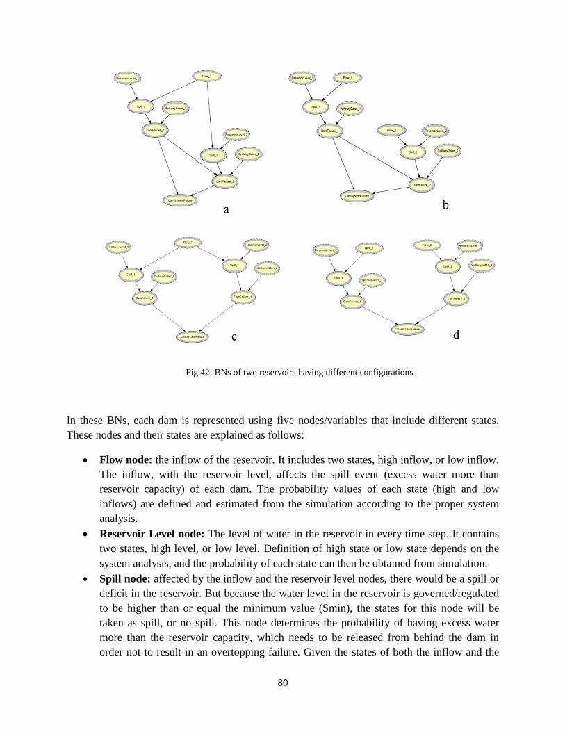
Fig.42 : BNs of two reservoirs having different configurations ………………………….. 80
Fig.43: BN of two reservoirs in series with dependent inflows…………………………… 81
Fig.44: BN of two reservoirs in series with independent inflows………………………… 82
Fig.45: BN of two reservoirs in parallel with dependent inflows…………………………. 82
Fig.46: BN of two reservoirs in parallel with independent inflows……………………….. 83
Fig.47: Probabilistic data and results of the BN of two reservoirs in series
with dependent inflows…………………………………………………………… 85
Fig.48: A cycle with n vertices [99]……………………………………………………….. 90
Fig.49: Directed Acyclic Graph (DAG)…………………………………………………… 91
Fig.50: Directed Acyclic Graph (yellow) of Directed Cyclic Graphs (blue)……………… 91
Fig.51: Markov Chain of three states S1, S2, S3............................................................. 93
Fig.52: A BN with a hidden Markov model [101]……………………………………….. 94
Fig.53: A BN structured hidden Markov model [101]…………………………………… 95
Fig.54a: A 23 node BN……………………………………………………………………. 97
Fig.54b: A 23 node BN being decomposed to 4 BN sub-networks……………………….. 97
Fig.55: Markov Chain of a three scenario BN sub-network………………………………. 98
Fig.56: Markov Chain of a two scenario BN sub-network……………………………….. 98
Fig.57a: A 17 node BN……………………………………………………………………. 100
Fig.57b: A 17 node BN, with every node includes two states (at least)…………………... 101
Fig.57c: A 17 node BN, with every node includes a two state Markov Chain……………. 101
Fig.58: Two state Markov Chain for every node………………………………………….. 102
Page 13
xiii
Fig.59: A BN of a three reservoir system…………………………………………………. 103
Fig.60: Three reservoir system BN decomposed to four sub-networks…………………… 104
Fig.61: General three reservoir BN, decomposed to four sub-networks………………….. 105
Fig.62: Markov Chain of a three scenario reservoir BN sub-network
(Overtopping, Sliding, or Seepage)………………………………………………. 106
Fig.63: BN of a three reservoir system, with every node includes a lower level
Markov Chain…………………………………………………………………….. 107
Fig.64: Higher level Markov Chain for the three reservoirs BN, MCSSBN
second approach………………………………………………………………….. 108
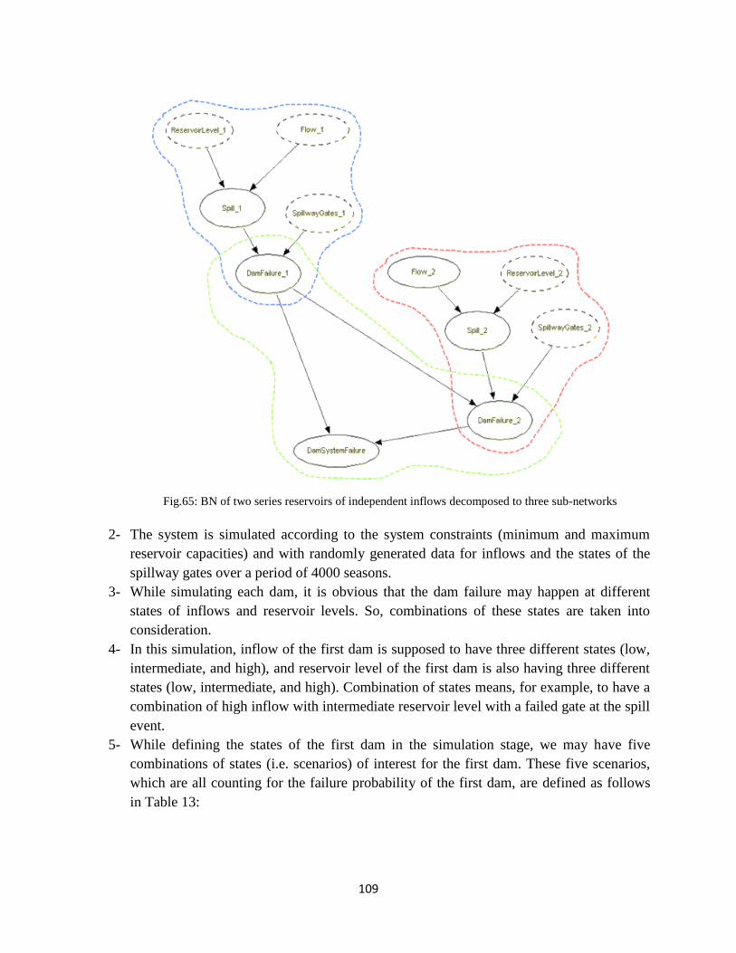
Fig.65: BN of two series reservoirs of independent inflows decomposed to
three sub-networks……………………………………………………………….. 109
Fig.66: An example of a Markov Chain for a five scenario BN
sub-network of the first reservoir………………………………………………… 111
Fig.67: Randomly generated Markov Chain for the five scenario BN
sub-network of the first reservoir………………………………………………… 112
Fig.68: An example of a Markov Chain for a seven scenario BN
sub-network of the second reservoir……………………………………………… 112
Fig.69: Randomly generated Markov Chain for the seven scenario
BN sub-network of the second reservoir…………………………………………. 113
Fig.70: Higher level BN for two reservoir system with three sub-networks……………….113
Fig.71: Higher level BN for two reservoir system in Hugin Lite………………………….. 114
Fig.72: The higher level BN given the evidence that system failure took place………….. 116
Fig.73: BN of two series reservoirs of independent inflows………………………………. 117
Fig.74: Randomly generated Markov Chain for the three state inflow of the
first dam…………………………………………………………………………... 118
Fig.75: Randomly generated Markov Chain for the four state inflow of the
second dam……………………………………………………………………….. 119
Fig.76: Randomly generated Markov Chain for the three state reservoir level
(storage) of the first dam………………………………………………………….. 119
Fig.77: Randomly generated Markov Chain for the three state reservoir level
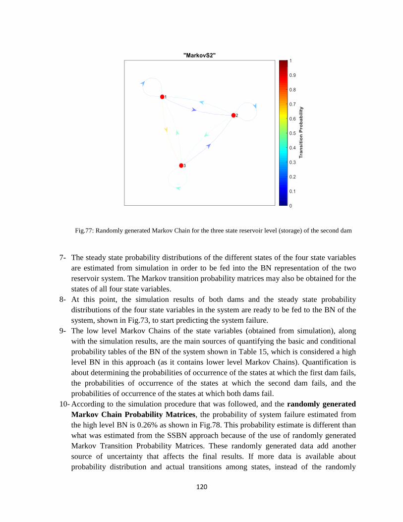
(storage) of the second dam………………………………………………………. 120
Fig.78: BN with failure probabilities of a system of two series independent
reservoirs using MCSSBN second approach……………………………………... 123
Fig.79: Main contributors to system failure of a system of two series reservoirs
using MCSSBN second approach………………………………………………… 124
Fig.80: Posterior probability of system failure given some evidences in a system
of two series reservoirs using MCSSBN second approach………………………. 124
Fig.81: Higher level scenario (combination of states) for the entire network……………. 125
Fig.82: An example of higher level Markov Chain showing
dynamic scenarios (combinations of states) for the entire network……………… 126
Page 14
xiv
Fig.83: BN of Mountain Chute dam and generating station……………………………… 131
Fig.84: BN of Mountain Chute dam after compilation on Hugin Lite……………………. 141
Fig.85: BN of Mountain Chute given the evidence that main dam failed………………… 142
Fig.86: BN of Mountain Chute given the evidence of normal/safe operating conditions…. 143
Fig.87: Mountain Chute Dam and Generating Station (sluiceway and sluice
gates to the left)………………………………………………………………….. 144
Fig.88: Side view of the sluiceway and sluice gates of Mountain Chute dam…………….. 144
Fig.89: Collecting point of drainage in the main dam body……………………………….. 145
Fig.90: Controlled vegetation around the main concrete dam…………………………….. 145
Fig.91: One of the earthen block dams (behind the trees)…………………………………. 146
Fig.92: BN of Mountain Chute dam using expert engineering judgement
for quantification…………………………………………………………………. 149
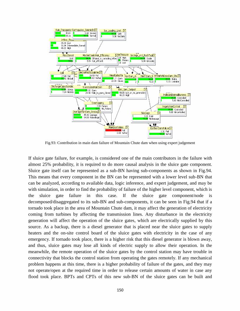
Fig.93: Contribution in main dam failure of Mountain Chute dam when
using expert judgement…………………………………………………………… 150
Fig.94: Sluice Gate node decomposed to its sub-BN and sub-components……………….. 151
Fig.95: BN of Mountain Chute decomposed to four sub-networks……………………….. 152
Page 15
xv
List of Tables
Table Page no.
Table 1: Different types of radionuclide with their half-lives [13]………………………. 8
Table 2: Geological Regions in Canada………………………………………………….. 14
Table 3: Comparison of BN, ETA, FTA, and Simulation………………………………… 35, 36
Table 4: Average seasonal temperature difference between surface and 500m depth…… 47
Table 5: Selected values of bentonite dry density versus probability of
bacterial activity………………………………………………………………… 48
Table 6: Change in RH from surface to 500 m depth in different seasons……………….. 49
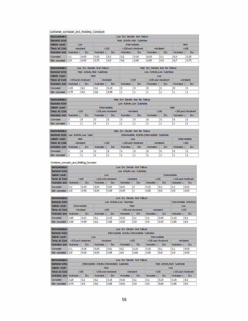
Table 7: BPTs and CPTs for the proposed BN………………………………….... 54, 55, 56, 57
Table 8: Simulation results for two reservoir system with different configurations……… 78
Table 9: BPTs and CPTs for the BN representation of two reservoirs in series
with dependent inflows, using probability estimates from simulation…………. 84
Table 10: BN results for a two reservoir system with different configurations, fed
from simulation (SSBN)………………………………………………………… 85
Table 11: Effect of increased number of states on the SSBN results for a system
of two dams……………………………………………………………………. 86
Table 12: Predicting failure probabilities for future time periods from SSBN steady
state estimates…………………………………………………………………… 87
Table 13: Scenarios of the first dam reservoir…………………………………………….. 110
Table 14: Basic and Conditional Probability Tables for the higher level BN
for two dam reservoirs………………………………………………………….. 115
Table 15: BPTs and CPTs of MCSSBN second approach for two series
dam reservoirs of independent inflow ………………………….……............121, 122
Table 16: Comparing probability of system failure using different
methods: simulation, SSBN, and MCSSBN………………………………….. 127
Table 17: BPTs and CPTs of the BN of Mountain Chute dam…………….......135, 136, 137, 138
Page 16
xvi
List of Abbreviations
ASCE: American Society of Civil Engineers
BN: Bayesian Network
BNA: Bayesian Network Analysis
BPT: Basic Probability Table
CPT: Conditional Probability Table
CNSC: Canadian Nuclear Safety Commission
DAG: Directed Acyclic Graph
DGR: Deep Geological Repository
DSM: Dam Safety Management
ETA: Event Tree Analysis
FTA: Fault Tree Analysis
FMEA: Failure Modes and Effects Analysis
GHGs: Green House Gases
GSC: Geological Survey of Canada
HCB: Highly Compacted Bentonite
HLW: High Level radioactive Waste
HRT: Head Race Tunnel
IAEA: International Atomic Energy Agency
ICOLD: International Commission on Large
Dams
IDF: Inflow Design Flood
IRB: Iron-Reducing Bacteria
LOL: Loss of Life
MA: Markov Analysis
MCS: Monte Carlo Simulation
MCMC: Markov Chain Monte Carlo
MCSSBN: Markov Chain Simulation Supported
Bayesian Network
NSDF: Near Surface Disposal Facility
NWM: Nuclear Waste Management
NWMO: Nuclear Waste Management
Organization
OPG: Ontario Power Generation
PAR: Population at Risk
PDF: Probability Density Function
PFA: Probabilistic Failure Analysis
PMP: Probable Maximum Precipitation
PRA: Probabilistic Risk Assessment
RH: Relative Humidity
RoR: Run of the River
SSBN: Simulation Supported Bayesian Network
SHPD: Safety of Hydropower Dams
SRB: Sulphate-Reducing Bacteria
TRT: Tail Race Tunnel
TPM: Transition Probability Matrix
UFC: Used Fuel Container
Page 17
xvii
List of Symbols and Units
Unit Symbol
Name
Quantity
Sv
Sievert
Equivalent/ Effective Radiation Dose
Bq
Becquerel
Radioactivity
°C
Degree Celsius
Temperature
°F
Degree Fahrenheit
Temperature
kg
Kilogram
Mass
km
Kilometer
Length
S
Second
Time
m3
cubic meter
Volume
Pa
Pascal
Pressure
MPa
Mega Pascal
Pressure
N
Newton
Force
kW
Kilo Watt
Electric Power
MW
Mega Watt
Electric Power
kWh
Kilo Watt hour
Electric Energy
MVA
Mega Volt Ampere
Apparent Electric Power
Page 18
1
CHAPTER 1
Introduction, Problem Definition, and Hypothesis
Page 19
2
1.1 Introduction
Failure analysis is an important and challenging aspect of the study of complex systems. A
system is defined to be consisting of components, sub-systems, inputs and outputs within system
boundaries. The inputs provide physical resources and information to the sub-systems, which are
interacting among each other to produce some outputs. All interactions are assumed to take place
within system boundaries. A complex system can be defined as a system structure that is
composed of many components that have complex interactions, [1]. Any failure in performing
the required interactions among system components or any failure in getting the expected
output/result is considered to be contributing to system failure, [2]. Thus, analysis of a system
with its components is a crucial step in determining the difficulties and complexities that the
system will experience at any stage. However, in the real world, performance of both inputs and
sub-systems is affected by probabilistic uncertainty, and hence a failure may come with an
associated probability. Probabilistic uncertainty due to randomness of events or values and
limited knowledge are considered main sources of uncertainty in systems introduced in this
thesis, [3, 4]. The main goal of this research is to evaluate the probability of failure of complex
systems, while finding the failure causes, and hence the analysis is called the probabilistic failure
analysis (PFA). For any given system with its inputs and sub-systems, probabilistic failure
analysis depends on finding the probability of not getting the required or estimated output of that
system. The required output may be the effect that is produced from certain causes (i.e.
prediction reasoning), or the determination of the cause responsible for certain results and effects
(i.e. diagnostic reasoning). Thus, determining the cause-effect relation is an important first step
in the probabilistic failure analysis, which allows for better understanding to enhance the system
reliability and take decisions for mitigating the negative effects or better enhancing the causes.
In this research, the concept of probabilistic failure analysis is applied to two main real-world
case studies: 1- Nuclear Waste Management (NWM), and 2- Safety of Hydropower Dams
(SHPD). The type and complexity level varies in these two case studies; however, both can be
analysed as “Complex Systems”. For each case study, relevant literature is reviewed to
understand the problem, study existing solutions, and determine system factors, parameters, and
variables. As a result, the system can be represented graphically. Lastly, probability measures are
applied to each system’s graphical network to estimate the probability of failure for given
scenarios/situations. In this thesis, the graph representation of both systems is conducted using
Bayesian Networks (BNs) which allow for representing marginal, conditional, and joint
probability measures affecting system components. Representing systems of engineering
applications using BNs is affected by multiple factors that affect the probabilistic quantification
process. The aim of this thesis is to develop approaches that facilitate the probabilistic
quantification of BNs, and hence, facilitate prediction of system failures, as follows:
1- Incorporating simulation of the entire system with the BN representation, given that
simulation may be challenging especially for very complex systems that include a huge
number of system variables. This approach is named “Simulation Supported Bayesian
Network (SSBN)” in this thesis. In this approach, simulation is used as a source of
probabilistic information that is used to quantify the basic nodes and conditional relations
among system nodes/variables, and
2- Incorporating Markov Chains to the SSBN approach, named “Markov Chain Simulation
Supported Bayesian Network (MCSSBN)” in this thesis. This approach is supposed to
overcome the limitation of being acyclic in the BN representation of the system. This
Page 20
3
allows for cyclic system analysis for different system scenarios/situations, and easy
update for the system in case any new data becomes available.
1.2 Problem Definition
Failure analysis of complex engineering systems is challenging for different reasons. Most of the
complex systems include multiple factors and variables of different natures (i.e. technical and
non-technical). These factors are mostly associated with probabilistic measures which lead to the
requirement to represent marginal, joint, and conditional probabilities of the events contributing
to any system failure, resulting in probabilistic uncertainty. Current practices use exhaustive
simulation models, which may be computationally intensive when dealing with any complex
system of a huge number of system components, complex interrelations, and/or nonlinear
governing equations. This makes the probabilistic representation for system failure analysis not
easy to interpret. Failure analysis of these systems is important in the sense that how likely they
will reach a failure state (probability of failure) and what will be the consequences of failure in
terms of expected loss or other probabilistic measures quantifying those consequences, e.g.
vulnerability, reliability and resilience. Estimating the probability of failure in such systems
could be hard because the state of the systems is a vector of multiple stochastic variables having
a huge number of possible values in a multidimensional state space. Particularly, when a failure
state results from multiple factors, this means that the probability of failure would be a joint
probability function of multiple variables and events. Knowing that the relationships between
input and output vectors of variables is complex, it would be practically impossible to determine
the joint probability function of output vector analytically even if the probability function of
input vectors are simply Gaussian and statistically independent, whereas in general the
distributions are non-Gaussian and dependent. Hydropower dams and nuclear waste management
using deep geological repository systems may be good examples of complex systems that have
multiple interrelated factors. Dam systems are complex systems having a huge number of
interacting factors and components. The deep geological repository system is also complex in
terms of the interactions among system components and the lack of operational data for such
future projects. In such systems, exhaustive simulations are challenging while predicting any
system failure, and while diagnosing the causes of such failure. Decision makers in charge of
such systems need a multifactor representation to overcome the challenges of current practices
and to facilitate interpreting the interrelations among system components while predicting the
failures or diagnosing the failure causes in terms of probability estimates during different
situations/scenarios. Data scarcity is one major factor that makes the risk analysis of such
systems challenging. A rational framework to analyze failures and risks of these systems is
crucial in both the short terms and the long terms and BN provides the foundation for such
framework. It is shown later in this thesis that Bayesian Networks (BNs) have potentials that
help solving such problems. Bayesian Network provides a graphical representation of any system
using basic probabilities, for system inputs, and conditional (transition) probabilities, for sub-
systems and their mutual interactions. There are some advantages and limitations in using BNs.
One of the main advantages is that BNs can integrate all types of data (e.g. social, environmental,
technical, etc.) because of the probabilistic nature of the BNs, as everything is represented as a
probability. Data must also be available to be able to estimate probabilities. This is not feasible
for systems which are still under research or will be applied in the future. However, BN analysis
Page 21
4
allows for integrating subjective probabilistic information and/or simulations, which can be
improved with additional data updates, when available. The main limitation is the acyclic
behaviour of the BN that doesn’t allow for analysis of systems with cyclic behavior that is
needed in some applications. When the system is fully represented by BN, the failure probability
could be estimated using Bayesian inference. Alternatively, BNs may be used to evaluate the
performance of the system components and their interactions to get some information about the
failure causes. If the post failure analysis stage is taken into consideration, determination of
causes and mitigation or treatment actions should be considered in order to improve the
performance and limit the overall system failure that the system may experience in the future. In
this research, two case studies are used to develop Probabilistic Failure Analysis (PFA) for
complex systems: 1- is for high level radioactive Nuclear Waste Management (NWM), which is
still a future project under development, and 2- is to analyse Safety of Hydropower Dams
(SHPD), whose risks of failure include failure probability, and consequences of failure. For the
purpose of this thesis, we are focussing mainly on the first part (i.e. failure probability) with
some extensions to be provided for the second part (i.e. consequences) in the future. The two
case studies are totally different in terms of application, but they are both complex systems and
can be represented probabilistically, but the main challenge is the data type. In NWM, which is
still a blue print, only partial data for this system or its components are available and requires
detailed simulations, which are outside of the scope of this thesis. On the other hand, SHPD is a
known problem with known technical databases but with a significantly larger number of
components than NWM, thus having large data requirements. In this thesis, the BN is used as a
multifactor representation for complex systems in order to predict system failures and diagnose
failure causes. In case of data scarcity, BN representation may integrate simulation and/or
subjective probabilistic information to facilitate the failure analysis. This research presents
methodologies utilizing Simulation and Bayesian and Markovian Networks for predicting
probabilities of failures of complex systems, using information of system components and their
interconnections.
1.3 Hypothesis and Proposed Methodology
In this research, failure is analyzed for two complex systems:
1- NWM (Nuclear Waste Management) using deep geological repository for high level
radioactive waste (spent nuclear fuel) management, and
2- SHPD (Safety of Hydro Power Dams), a pilot study of a two dam reservoir system is
identified for applying the proposed methodologies. Then, a real-world case study for one
of the dams operated by Ontario Power Generation (OPG) is used to apply the proposed
methodology, with the restriction of availability of operational data.
Firstly, in Chapter 2, the literature explaining both systems and their problems are reviewed.
Then, the different factors affecting the system failure in both of them are illustrated. Knowing
the different components, factors, parameters, and sub-systems for any system will facilitate the
task of constructing a graphical representation for the specified system. As Bayesian Networks
(BNs) have shown some advantages in representing any system as a probabilistic graphical
network, BNs are used extensively in this research. Chapter 3 uses the data available for the
different components of NWM case study to build the system’s BN. Once the graph of the
Page 22
5
system is constructed, the data available are used to quantify the probabilities of the BN nodes
and their interactions (basic and conditional probabilities). Depending on different scenarios, or
change in data from location to another (in case of the deep geological repository), or from time
to time (for the operation of dams in different seasonal conditions), the probabilities may change
resulting in increasing or decreasing the failure probability. Thus, there is a need to compile the
BN of such systems to obtain the joint and marginal probabilities related to certain situations or
events. To facilitate this task, Hugin Lite software was found to help in the representation of the
BN and its compilation [5, 6, 7]. So, the BN is constructed and all the data and scenarios are
inserted in order to start the compilation of cause-effect probabilistic analysis, resulting from
interrelating system components, and affecting the failure. While the BN representation for
failure prediction is dependent on available data in both applications, it is shown that failure
prediction is challenging. Probabilistic quantification relies on different sources of data, i.e.
expert judgement, logic inference, elicitation, empirical models, and simulation, which result in
different levels of inaccuracy in the estimated failure probability, which may be used for decision
making. In Chapter 4, the approach of incorporating simulation to the BN (SSBN) is introduced
and applied to a pilot two reservoir system. The decompositional approach used for simulating
complex systems – proposed in this thesis – is introduced as a part of the SSBN method. SSBN
is expected to reduce the limitation of exhaustive simulation that may be computationally
expensive in some applications. In Chapter 5, another approach that uses Markov Chains to be
incorporated with simulation and BNs to better quantify the probabilities of the system nodes and
their conditional relationships is introduced and applied to the same two reservoir system.
Markov Chain Simulation Supported Bayesian Networks (MCSSBNs) are proposed to make the
analysis cyclic and more dynamic while introducing different system scenarios/situations, and
allow for seamless update of the system with any new available information/data that could
affect the prediction process of system failure. As data and mathematical models are not fully
available for the real-world case study, as may be expected in most cases today, Chapter 6
illustrates how the elicitation of expert judgement and logic inference is used for quantifying the
BN of Mountain Chute Dam and Generating Station, operated by OPG, to predict its probability
of failure. Finally, in Chapter 7, conclusions are presented regarding the proposed
methodologies and their potentials and limitations in representing complex systems and
predicting their failure probabilities. Some recommendations are also suggested. The main focus
of the proposed research in this thesis is on the stage of failure prediction. In addition, the work
proposed in this research may help in identifying causes of failures by using diagnostic
capabilities of BN analysis.
Page 23
6
CHAPTER 2
Literature Review
Page 24
7
2.1 Introduction
This chapter provides a review of literature for the case studies used in this research. For the first
case study-Nuclear Waste Management (NWM) system, different factors that affect the system
are discussed. A brief description is also provided for the second case study of this research-
Safety of Hydropower Dams (SHPD) system. This chapter also provides an introduction to risk,
reliability, and uncertainty. The concept of Bayesian Networks is explained in details. Then a
comparison between BNs and other techniques, used for representing systems, is conducted.
2.2 Nuclear Waste Management (NWM)
Disposal is the final stage of the radioactive waste management by which the wastes are isolated
from biosphere in the repositories. For the disposal of radioactive solid wastes, multi-barrier
approach may be followed. If suitable engineered barriers, backfill materials and the
characteristics of the geo-environment of the repository site are properly selected, safety against
radionuclide migration will be achieved. Disposal of radioactive solid wastes depends on the
nature and type of radionuclide present in the wastes (longevity) and its concentration. Thus, the
repository can be near-surface or in deep geological formations. For long lived high level
radioactive wastes, deep geological repository (DGR) is the option, for disposal of used nuclear
fuel and high-level radioactive waste, which has received world-wide attention and may be the
best known method to do that permanently without putting a burden of continued care on future
generations. The option of Near Surface Disposal Facilities (NSDF) is preferred for low and
intermediate level radioactive wastes with comparatively large volumes, which arise during
nuclear power plant operation, and from radionuclide applications in hospitals and research
establishments. At NSDF, wastes are normally disposed in a depth around 50 meters
(intermediate depth). In NSDF, sub-surface evaluation is carried out systematically by geological
and geo-hydrological investigations. Testing of full scale engineered barriers should be
conducted for bentonite clay buffers and clay sand as backfill materials in both deep geological
repositories and near surface disposal facilities. It is believed that setting up dependency
relationships among the geological, hydrological, and ecological aspects will reduce the sources
of uncertainty in this area of research [8, 9, 10, 11].
Canada, like many nuclear nations, has been investigating geological disposal of nuclear waste,
which is the approach that offers the best passive safety system for permanent disposal, since the
early 1970s. The internationally accepted design of a deep geologic repository (DGR) involves
the following [12], see Fig.1:
1. At depth of 500 meters below ground surface in a suitable location of dense intact rock,
used fuel will be disposed.
2. Nuclear spent fuel will be sealed in a corrosion resistant used fuel container (UFC). This
container should withstand anticipated hydrostatic, lithostatic and glaciation loads. The
original Canadian UFC, which is dual-walled with an inner iron (or steel) vessel to
Page 25
8
provide strength, and a separately fabricated 3 mm-thick copper coated outer shell
corrosion barrier, was designed to contain about 48 CANDU fuel bundles.
3. As an additional barrier, compacted bentonite clay will be surrounding the UFC.
Compacted bentonite clay swells on contact with moisture. This will tightly seal the
system with allowing very little chemical diffusion to occur.
In [10], a full explanation of the definitions and decrees (by Finnish government), regarding the
disposal of nuclear waste, is discussed. Spent nuclear fuel (which is considered high level
radioactive waste), along with low and intermediate level wastes are accumulated during the
operation and decommissioning of nuclear power plants. Spent nuclear fuel is intended to be
disposed in deep geological repositories, inside the bedrock, after being encapsulated. Selecting
and characterising the disposal site, developing disposal technology, collecting necessary data
for long term safety, excavation works, packaging the wastes and transferring the packages to
emplacement rooms, and the engineered barriers installation, are required stages in the disposal
process. According to Finnish government decrees, disposal facility shall be designed to have the
average annual dose to the most exposed individuals of the population not to exceed 0.01 mSv
during normal operation of the facility, with maximum of 5 mSv in the event of certain
accidents. Also in [10], exact and detailed definitions are given to: Low level waste (activity
concentration not more than 1 MBq/kg.), Intermediate level waste (1 MBq/kg –10 GBq/kg),
High level waste (>10 GBq/kg), Short-lived waste (less than 100 MBq/kg after 500 years),
Long-lived waste (more than 100 MBq/kg after 500 years), disposal facility, disposal site, and
barrier (engineered or natural). In [13], some definitions and management actions regarding
radioactive wastes are provided. The radioactive properties of radioactive wastes contains the
type of radionuclides, the radiation emitted (alpha, beta, gamma), the activity level (number of
atomic nuclei disintegrating per unit time, expressed in becquerels), and the radioactive half-life
(i.e. time taken by a radioactive sample to lose half of its activity). Short-lived radioactive waste
contains radionuclides with a half-life of less than 31 years, while long-lived radioactive waste
contains radionuclides with a half-life of over 31 years. See Table1.
Radionuclide Half-life
Cobalt-60 5.2 years
Tritium 12.2 years
Strontium-90 28.1 years
Caesium-137 30 years
Americium-241 432 years
Radium-226 1,600 years
Carbon-14 5,730 years
Plutonium-239 24,110 years
Neptunium-237 2,140,000 years
Iodine-129 15,700,000 years
Uranium-238 4,470,000,000 years
Table 1: Different types of radionuclide with their half-lives [13]
Page 26
9
The following engineered barriers should be considered in planning the waste disposal [10]:
1- The waste matrix;
2- The waste package;
3- The buffer surrounding the waste packages;
4- The backfilling of emplacement rooms; and
5- The closing structures of the disposal facility.
The bedrock of the disposal site is considered to be a natural barrier that lends support to safety
functions, but, there are also some factors that indicate the unsuitability of a disposal site [10]:
1- Proximity to natural resources;
2- High rock stresses;
3- High seismic or tectonic activity; and
4- Adverse groundwater characteristics,
Fig.1: Final Disposal Facility for spent nuclear fuel (High Level Waste HLW) [14]
In Canada, Nuclear Safety and Control Act (2000) created the Canadian Nuclear Safety
Commission (CNSC), Canada’s single nuclear regulator to regulate all nuclear-related facilities
and activities, from cradle to grave. CNSC, which is an independent commission, makes
continuous updates for its regulations regarding nuclear activities including regulations of safe
spent fuel and radioactive waste management. Nuclear Fuel Waste Act (2002), which established
a framework for national long-term management solution respecting Canada’s spent fuel, created
the Nuclear Waste Management Organization (NWMO) as a not-for-profit corporation funded
by waste producers. In the Government of Canada Radioactive Waste Policy Framework (1996),
both the federal government and waste producers and owners have responsibilities towards the
radioactive waste problem, [15]. Full details for nuclear waste management program in Canada
Page 27
10
are provided in [16], with understanding the fact that high level radioactive waste can stay in the
wet storage (in pools) for 7-10 years, and in dry storage for up to 70 years before being disposed
into deep geological repository (DGR). International Atomic Energy Agency (IAEA) provides
all the safety standards, in the disposal of radioactive waste, for protecting people and the
environment. Emplacing radioactive waste in a facility or location with no intention to retrieve
the waste is called “disposal” of radioactive waste. The lack of intention to retrieve wastes
doesn’t mean that retrieval is not possible. This is different than the term “storage”, which means
the retention of the radioactive waste with having retrieval intention. Both, disposal and storage,
aim at containing the waste and isolating it from accessible biosphere. Thus, waste storage is
considered a temporary stage followed by future actions of conditioning, packaging, and final
disposal [17].
Figures 2, 3, and 4 give a representation for the problem under study. The used fuel bundle
(Fig.2) is placed in the container shown in Fig. 3. The container should contain an assembly of
48 fuel bundles. These bundles generate both radioactive heat and mass that can be transferred to
the surrounding and needs to be shielded. For that reason, the used fuel container is made of
steel, with an outer corrosion barrier of copper. Then, the container is placed in a buffer box
made of bentonite clay as another barrier. Many buffer boxes are placed in placement room
(Fig.4) in the repository, which is 500 meters deep, and separated by backfill material as an
additional barrier. Then the whole placement room is filled with gap fill material to fill the gap
with the rocks of the placement room.
Fig.2: ACR-1000 FUEL Bundle (~ 20 kg) [16]
Page 28
11
Fig.3: The conceptual container design Fig.4: Schematic representation of the proposed
for the disposal of Canadian high level Canadian Deep Geological Repository (DGR) [12]
nuclear waste [12]
Failure in nuclear systems is related to the emissions of radioactive nuclides, or possible
accidental releases of radioactivity, like the ones described in ref [18]. From the nuclear aspect,
risk can be defined to be an exceeding expectation of the magnitude of undesirable radioactive
releases (i.e. the product of probability of an accident/failure, and the consequence of this
accident). In probabilistic risk assessments, uncertainty measures arise due to both, lack of the
knowledge and stochastic features of system components. So, complex uncertainty propagation
may result in future potential risks. In the next sections, Bayesian Network is shown to be a
concept for reasoning complex uncertain problems, where network means a graphical model [9,
18]. In [19] and [20], different and effective waste management policies are investigated with
giving detailed explanation of the radioactive waste management process. An overview is given
in [21] of the nuclear data required to make a correct prediction of the source of radioactive
wastes, and the radiation doses in the different activities of: manufacturing, production, handling,
transport, recycling, transmuting, and storing of radioactive, or fissionable, materials.
2.3 Factors Affecting the NWM System Failure
The operation of NWM Deep Geological Repository system is to keep the used nuclear fuel
away from interacting with the surrounding environment by encapsulating the fuel bundles in
used fuel containers. The system is considered to fail when the used fuel container fails to
prevent any interaction between the nuclear bundles and the surrounding environment. In this
section, the different factors that affect the NWM system operation and failure are explained in
details.
Page 29
12
2.3.1 Temperature Effect (Geothermal Gradient)
Variation of surface air temperature, with the seasons and regional variations according to local
weather conditions, is a known fact. Thus, ventilation of current temperature in underground
openings may affect temperature variation [22]. In [23], the surface average temperatures in the
Canadian cities all over the year are demonstrated, with giving the maximum and minimum
annual temperatures based on weather data collected from 1981 to 2010. The numbers allow
comparing the average daily high and low temperatures for the 33 largest Canadian cities.
Temperature is known to increase with depth in the Earth influenced by the heat generated at
depth and transferred through rocks and sediment layers. This is called terrestrial heat flow
which is described by the following equation [24]:
𝑸𝒛 = ∆ 𝑻
𝛌 ∆𝐃 Eqn. 2.1
Where:
Qz = Heat flow per unit area in the vertical direction,
λ = Thermal conductivity, and
∆T/∆D = Geothermal gradient (difference in temperature / difference in depth).
Because of some data constraints in both heat flow and thermal conductivity, the principal basis
for calculating geothermal gradients depends on bottom-hole temperatures measured in
boreholes [24]:
𝐺𝑒𝑜𝑡ℎ𝑒𝑟𝑚𝑎𝑙 𝐺𝑟𝑒𝑎𝑑𝑖𝑒𝑛𝑡 =𝐹𝑜𝑟𝑚𝑎𝑡𝑖𝑜𝑛 𝑇𝑒𝑚𝑝𝑒𝑟𝑎𝑡𝑢𝑟𝑒 − 𝑀𝑒𝑎𝑛 𝐴𝑛𝑛𝑢𝑎𝑙 𝑆𝑢𝑟𝑓𝑎𝑐𝑒 𝑇𝑒𝑚𝑝𝑒𝑟𝑎𝑡𝑢𝑟𝑒
𝐹𝑜𝑟𝑚𝑎𝑡𝑖𝑜𝑛 𝐷𝑒𝑝𝑡ℎ
In Canada, geothermal favourability ranking, in areas with geothermal gradient data, is given in
[25]. It can be concluded that geothermal gradient falls in the range between 30 – 55 (°C / km).
In [26], Government of Canada (Environment Canada) provides Historical Climate Data for
different Canadian Provinces by which monthly data reports for Canadian provinces and cities
can be easily gotten. While [27] provides geothermal maps of Canada at different depths in
different locations within the Canadian geological regions. Globally, the average geothermal
gradient ranges between 25 – 29°C / km depth, with actual value of more than 55
°C / km depth
in some regions. According to the above mentioned information, the surface temperature will
affect the final temperature at the deep geological repository according to the average geothermal
gradient. Accordingly, and because the average seasonal surface temperature data is available, in
this research, the year is divided into three seasons: Winter (W), Spring Summer (SS), and Fall
(F). Each season is assumed to have average weather conditions within its period. The maximum
geothermal gradient that will be used in this study will be the 29°C / km depth (assuming that the
repository will not be built in any of the regions that have extreme temperature and geothermal
Page 30
13
conditions). However, for the post-closure processes in the repository, the surface temperature is
not showing significant effect or significant change in the temperature of the repository from
season to season. The reason behind that is because the radioactive decay coming from the used
fuel will be much higher than the change in the surface temperature. The radioactive heat decay
will be the most dominant temperature changing factor after closure of the repository. According
to NWMO, there are studies for five locations (three crystalline rocks, and two sedimentary
rocks) where the repository is supposed to be placed in one of them. The location that will be
selected should have an average surface temperature of 5°C, with 16
°C/km geothermal gradient;
in order to have about 12°C temperature at the repository (500 m depth) resulted from the surface
temperature. From another side, the maximum temperature at the surface of the used fuel
container should be at maximum of 100°C at any time during the radioactive decay. This means
that the radioactive decay may be responsible for more than 80°C of the temperature in the
repository, or at least at the surface of used fuel container.
2.3.2 Pressure Effect (Geostatic and Lithostatic Gradient)
Pressure increases with depth in the earth due to the increasing mass of the rock overburden. The
geostatic pressure at a given depth is the vertical pressure due to the weight of a column of rock
and the fluids contained in the rock above that depth. Lithostatic pressure is the vertical pressure
due to the weight of the rock only. Computing the pressure as a function of depth in a
homogeneous crust is a straightforward calculation:
𝐏 = 𝛒 𝐕 𝐠
𝐀= 𝛒 𝐠 𝐇 Eqn. 2.2
Where:
A (m2): surface area of the repository
ρ (Mass (M) /Volume (V) = kg/m3): the density of rocks (in case of lithostatic pressure), or the
summation of rock and water densities (in case of geostatic pressure), and M (kg) is the rock
mass (in case of lithostatic pressure), or the summation of rock and water masses (in case of
geostatic pressure),
V (m3): volume of the repository = A (surface area) * H (depth),
g (9.81 m/s2): gravitational acceleration, and
P (N/m2 = Pascal Pa): Lithostatic Pressure (in case of just rocks), or Geostatic Pressure (in case
of both rocks and fluids).
Higher rock densities will yield higher pressure gradients. The geostatic gradient changes with
depth as the density increases. This is called crustal geostatic gradient. In that order, to calculate
the pressure in the deep geological repository, it is important to know the densities of all the rock
types all over the country. According to [28], Canada can be divided into six geological regions:
The Canadian Shield, Interior Platform (Canadian Interior Plains including Hudson Bay Low
Lands), Appalachian Orogen (East), Eastern Continental Margin (St. Lawrence Low Lands),
Page 31
14
Innuitian Orogen (North Arctic Lands), and Cordilleran Orogen (Western Sedimentary Basin).
Each geological region has specific characteristics and different mineral resources (see Fig.5 and
Table 2).
Fig.5: Geological Regions of Canada [28]
Geological Region
Percentage of
Canada’s Area
The Canadian Shield ~50%
Interior Platform (Canadian Interior Plains including Hudson Bay Low Lands) ~22.5%
Appalachian Orogen (East) ~3.6%
Eastern Continental Margin (St. Lawrence Low Lands) ~1.8%
Innuitian Orogen (North Arctic Lands) ~5.4%
Cordilleran Orogen (Western Sedimentary Basin) ~16%
Table 2: Geological Regions in Canada
So, if the decision is not taken yet about the location of the repository, it will be impossible to
calculate the maximum effect that comes from the pressure factor. Thus, this led to considering
something else. The Earth crust contains both continental and oceanic parts. The oceanic crust
Page 32
15
counts for the seas, oceans, rivers, and lakes, while the continental crust accounts for the rest. In
Canada (9,984,000 km2), the continental crust counts for 92% of the Canadian Land, while the
oceanic counts for about 8%. The average density of continental crust is known to range between
2500-3000 kg/m3 (2.5-3 g/cm
3) according to the rock type. While the oceanic crust average
density ranges between 3-3.3 g/cm3 [29]. Accordingly, more realistic data can be estimated about
the maximum pressure that could be faced in case of building the repository beneath rocks or
under (or near) oceans and seas. Moreover, if there is ice accumulation at the location where the
repository is built, ice pressure should be taken into account (ice loading). Another factor, that
will affect the pressure in the repository, is the bentonite swelling pressure. The used fuel
container will be emplaced in a Highly Compacted Bentonite (HCB) buffer box. If the bentonite
is hydrated or gets wet at any time, it will swell to seal the buffer box and prevents any diffusion,
form inside to the outside or vice versa, from taking place. The swelling pressure of the bentonite
should be taken into consideration for calculating pressure on both the used fuel container, and
the walls of the emplacement room. In the five location that are being tested by NWMO, the total
of geostatic pressure and the bentonite swelling pressure should count for 15 MPa, while the ice
loading will count for at most 30 MPa. That is 45 MPa in total maximum pressure in the
repository.
2.3.3 Relative Humidity and Water Saturation
Relative humidity is the ratio of vapor pressure (mixing ratio) to the saturation vapor pressure
(saturation mixing ratio). Given by another definition, Relative Humidity is the ratio of the actual
amount of water vapor in a given volume of air to the amount which could be present if the air
was saturated at the same temperature. It is expressed as a percentage (percentage of saturation
humidity), and reaches 100% when the air is saturated with respect to water (the case of ice).
𝑹𝒆𝒍𝒂𝒕𝒊𝒗𝒆 𝑯𝒖𝒎𝒊𝒅𝒊𝒕𝒚 = 𝑨𝒄𝒕𝒖𝒂𝒍 𝑽𝒂𝒑𝒐𝒓 𝑫𝒆𝒏𝒔𝒊𝒕𝒚
𝑺𝒂𝒕𝒖𝒓𝒂𝒕𝒊𝒐𝒏 𝑽𝒂𝒑𝒐𝒓 𝑫𝒆𝒏𝒔𝒊𝒕𝒚 × 𝟏𝟎𝟎% Eqn. 2.3
At a given vapor pressure (or mixing ratio), relative humidity with respect to ice is higher than
that with respect to water. For unsaturated air, relative humidity is inversely proportional to the
temperature. Since warm air will hold more moisture than cold air, the percentage of relative
humidity must change with changes in air temperature. In that order, relative humidity doubles
with each 20 degree (Fahrenheit) decrease, or halves with each 20 degree increase in
temperature. Generally, as temperature goes up, relative humidity goes down and vice versa. Ref
[23] also demonstrates the average relative humidity in the Canadian cities all over the year, and
gives the morning and afternoon annual relative humidity averages based on weather data
collected from 1981 to 2010. The numbers allow comparing the average daily high and low
relative humidity for the 33 largest Canadian cities. It is obvious that the relative humidity
average never exceeds 95% at the surface, with having most of the big cities below the 88%.
Page 33
16
Relative humidity measures the actual amount of moisture in the air as a percentage of the
maximum amount of moisture the air can hold (saturation). Accordingly, at the repository, while
the temperature increases with going down in depth, the relative humidity should decrease. In the
post-closure conditions, the changes in surface temperature will not have significant effect on the
repository temperature, so, changes in surface relative humidity will not have significant effect
on the repository conditions as well. From the humidity saturation point of view, the dominant
factor in the post-closure case will not be the relative humidity, but rather, it will be the water
saturation in the repository. Having wet, humid, or hydrated contents of the repository will affect
the swelling conditions of the bentonite clay used to cover the used fuel containers, and may be
considered a water diffusion in the repository. Water diffusion may be taking place because of
the surrounding environment at the repository location, and may lead to corrosion factors for the
used fuel container. One example for the water diffusion and water saturation is the groundwater
in case it is present at any stage in the repository post-closure life time. The salinity level of the
groundwater may affect the bacterial activity, and the corrosion factors of the used fuel
containers. In summary, the water diffusion, which leads to swelling pressure, will affect the
bentonite clay surrounding the containers (according to its density or compaction factors), and is
affecting the bacterial activity levels around the containers. If bacterial activity is present in the
repository, this leads to increasing sulphide levels, which is considered the main corrodent for
the used fuel containers. Thus, proximity to hydrological resources is another measure that
should be taken into consideration, means, how far the repository is from hydrological
resources?
Proximity to hydrological resources means that the probability of having water diffusion from
outside the repository to its inside may take place because of the underground water resources
(that is generated from sea, ocean, or precipitation infiltration). Groundwater flows through
aquifers, which are geological formations made up of granular or fractured material from which
a sufficient quantity of water can be extracted to serve as a water supply. According to [30], the
first sub-question that should be asked in this case is “What current knowledge gaps limit our
ability to evaluate the quantity of the resource, its locations and the uncertainties associated with
these evaluations?”. Accurate estimates of the volume of groundwater in Canada were
impossible to be identified. The Geological Survey of Canada (GSC) stated that, according to
[30], “the amount of groundwater stored in Canadian aquifers and their sustainable yield and role
in ecosystem functioning are virtually unknown”. In another meaning, the groundwater
consumption in Canada is known, but the actual volume is unknown. Because of that, the
proximity to hydrological resources will be determined from being located in or near to the
regions having oceanic crust (which is about 8% of Canada). As a result, if the repository is
located in a continental crust region, it may be assumed to be far away from underground
hydrological resources. However, for the locations that are being tested by NWMO, precautions
will be taken to locate the repository in an area that is known for low groundwater amounts, or to
be far away from the groundwater aquifers. If the repository is chosen to be in a groundwater
Page 34
17
existing location, it should be of low salinity levels and low concentration of potentially
corrosive agents.
2.3.4 Bacterial (Microbial) activity
The sulfide content and salinity level of the bedrock, in which the repository will be located,
represent a crucial factor. Sulfides and salinity are influencing the corrosion process of metals
contained in the repository (spent fuel waste metal containers). Salinity level is different for
every rock type, and may exist because of the water diffusion coming from groundwater, which
have different salinity levels depending on the aquifers. Bacterial (or microbial) activity is
affected by salinity, as with the salinity increases, the bacterial activity decreases, and vice versa.
If bacteria are active, this will result in sulphide content, and sulphide is considered a corrodent
to metals. Thus, in the bedrock, in which the repository will be located, the existence of
microbial or bacterial activity affects the corrosion level of the metal containers. Moreover, if the
salinity increases, the tendency of metals to corrode also increases. So, care should be taken
when deciding which rock type and bedrock in which the repository will be built, as choosing a
saline rock type will decrease the bacterial activity in the repository, but will increase the salinity
level in the repository, and then, increases the metal tendency to corrode, and vice versa.
Moreover, regular measures and field data should be available in order to realize the amount of
activity of the microbes and bacteria, as the microorganisms’ life transform from phase to phase
over time. In that order, the locations, which are being tested by NWMO, should be chosen to
have low salinity levels and low concentration of potentially corrosive agents. And in order to
achieve that, locations of low salinity levels will be chosen, along with limiting the bacterial
activity with maintaining high pressure values in the repository in order to prevent the bacteria
from being active, and thus, not producing sulphides. For that reason, the compacted bentonite
clay used to surround the container should have high dry density, in order to reduce the bacterial
activity in the dry phase. While in the wet case, when having humidity, water diffusion, or water
saturation, the swelling pressure of the bentonite, of high dry density, will do the job of
preventing the bacteria from being active, and limit the existence of free water (bacterial growth
increases in free water). This will lower the sulphide contents in the repository, and thus,
reducing the tendency of metal corrosion of the used fuel containers.
2.3.5 Corrosion and Welding Corrosion of the Used Fuel Containers (UFCs)
Corrosion of the containers, in which the spent fuel assemblies (which assemble the fuel
bundles) are emplaced, is an important factor that may affect the diffusion analysis in case the
failure happens. According to [12] and [31], at a depth of about 500 m in bedrock, where the
spent fuel will be deposited in the repository, the waste canister provides safety during handling
and emplacement of the waste in the repository. It also ensures complete isolation of the waste
for a desired period of time (minimum of 500-1000 years) during which most of the important
fission products will decay, and the heat generation (by radioactive decay) of the waste is most
Page 35
18
important. This temperature rise will result in a low humidity environment in the vicinity of the
container (lowering expectation of corrosion). After emplacing the canister in the emplacement
room, the room will be sealed with bentonite clay mixture. The dimensions and waste load of
each canister, which is double walled with thickness that acts as a radiation shield, have been
chosen such that the temperature on the outer surface of the canister never exceeds 100° C. The
external pressure in the repository may reach the value of 15 MPa resulting from a 5 MPa
hydrostatic pressure and maximum of 10 MPa bentonite swelling pressure. In [31], corrosion is
discussed deeply: corrosion by oxygen (aerobic corrosion), corrosion by sulfides (anaerobic
corrosion), and other types of corrosion and how they may affect the canister and its welding
over time. The sulphides, which act as the main corrodents, can be supplied from the buffer
mass/backfill in deposition holes and tunnels as well as from the groundwater. In addition to
these sources, it can also be produced from sulphates through microbial activity. In order to face
all these types of corrosion, copper was chosen to be the coating material of the canister, and
presented as a reference canister material, because of its thermodynamic stability in pure water.
In the Canadian repository, corrosion conditions will be taken initially to be aggressive and
extreme until reaching a benign state [12]. Another aspect to be determined, what if the container
is emplaced in the repository with a through-coating defect (in the copper coating or welding)?
Obviously, this situation can be avoided by proper inspection of the container prior to
emplacement, but failure to detect defects will be considered [12]. So, this arouses the need to
know the factors influencing the corrosion of weldments, which may be one or more of the
following [32]: weldment design, fabrication technique, welding practice, welding sequence,
moisture contamination, organic or inorganic chemical species, oxide film and scale, weld slag
and spatter, incomplete weld penetration or fusion, porosity, cracks (crevices), high residual
stresses, improper choice of filler metal, or final surface finish. This means that if the welding
technology has any of the above problems, there may be some weak points present in the weld,
which will definitely be followed by a failure in the canister. Fig.6 shows the UFC coating.
Fig.6: Spent fuel container and its coating [33]
Page 36
19
2.3.6 Bentonite Clay (Buffer Boxes, Gap Fills, and Back Fills)
Canada, China, Belgium, France, Germany, Japan, Sweden, and many other countries have
considered deep geological repository for high-level radioactive waste (HLW). In present design
concepts, compacted bentonite-based materials are supposed to be used as sealing/buffer
materials in the emplacement rooms of the deep geological repository of the high level
radioactive wastes (nuclear spent fuel) due to their low permeability, high swelling capacity, and
high radionuclide retardation capacity [34]. It is also supposed to use bentonite clay as a back fill
material in the repository. A fundamental property of bentonite is that when it absorbs water, it
expands. However, not all bentonites have the same absorption capacity. According to [35],
thermal treatment of bentonite (up to 400°C) drastically reduces its swelling behavior. In [36],
bentonite clay is evaluated as an alternative sealing material in oil and gas wells. As compared to
cement, which has the tendency to shrink, bentonite shows superior sealing ability during
hydration (as it swells and expands). Along with that, it has lower permeability, than cement,
during hydration, with the ability to reshape itself and heal any cracks which may occur during
subsurface movements. In [37], swelling test (swelling pressure test) and hydraulic conductivity
test are performed for bentonite clay under the same conditions of deep geological repository.
This work was conducted because the bentonite clay showed high swelling capacity, and good
durability under disposal environment, so that the penetration of groundwater from the host
environment can be minimized. After closing the emplacement rooms, under hydration
conditions, bentonite will swell to fill the gaps among the bentonite bricks (i.e. buffer boxes),
between the canister and the buffer box, between buffer box and the host rock, and fills the
fractures in the host rock due to excavation. After that, the subsequent swelling is restrained by
the host rock and swelling pressure is developed (this pressure must be lower than certain limits).
Fig.7, Fig.8, and Fig.9 show the bentonite buffer box and the placement room. Thus, proper
understanding of the behaviour of compacted bentonite-based materials during hydration is vital
for determining short and long term performance of the deep geological repository, [34].
Fig.7: Bentonite Buffer box [33] Fig.8: Placement Room Concept [33]
Page 37
20
Fig.9: Placement Room (side view)
2.4 Safety of Hydropower Dams (SHPD)
Dams are of different types and techniques of operation. In this research, many types of dams
can be considered for the application of the proposed failure prediction approaches that are
explained in the next chapters. However, embankment dams, which include both earthen and
rockfill dams, are the main type that is reviewed in this section.
In [38], a procedure for incorporating the risk of catastrophic failure in project evaluation is
presented. The evaluation of risk depends mainly on estimating the probability of failure. So, the
main challenge is how to determine the probability of failure of dams or dam systems. The
different factors affecting the failure of dams are briefly explained in the next section.
2.4.1 Factors Affecting the SHPD System Failure
Dams are complex engineering structures that incorporate huge number of interacting system
components. Failure in dam systems depends on failure in performing the required interactions
among system components, and/or failure to achieve at least one of the required system
outputs/results. In this section, the different factors, related to the SHPD system operation and
failure, are reviewed.
2.4.1.1 Hydrological Factors
Dams are used for controlling and/or storing water for different purposes, which mean that water
is the main factor affecting dams’ operation. The hydrological factors are mainly the inflow to
the dam, the water storage, and the outflow from the dam. The water inflow to any dam is
affected by upstream events, i.e. precipitation, flood, or connection to any upstream dams.
Depending on the inflow rate to the dam, water is stored in the dam reservoir and/or released to
the downstream of the dam by water management techniques (i.e. gates). If the water inflow
results in exceeding the maximum capacity that the reservoir can hold, there is a requirement to
Page 38
21
spill, and the extra amounts of water should be released using spillway gates. In hydropower
dams, water is also released from the hydropower turbines after generating electric power using
the head difference between upstream and downstream water levels. Failure in dam reservoir
operations is considered a failure of the dam system.
2.4.1.2 Structural and Design Factors
Dams are of different types like embankment dams, arch dams, gravity dams, saddle dams,
buttress dams, coffer dams, and diversion dams, amongst other types. In every type, there are
different designs and different operating conditions. The type of the dam, its design, and the
structural aspects play an important role in dam failure. This section presents a review of some
literature on structural and design aspects that affect the failure of dams, especially embankment
dams, as they are the most widely used dams in the world involved in the most historical dam
failure events, including breaching.
For dam failures, the input breaching characteristics, which are dependent on breach formation
mechanisms, are presented in references [39] and [40].
In general, amounts of data reported for dam failures are minimum, which limits the assessment
studies (qualitative and quantitative) for dam breaches and failures. One type of the important
data is the embankment dam characteristics, which includes size and shape of the embankment,
cohesion of embankment material, embankment zoning (zones’ type, size, and number), and
foundation geology [39, 41]. Availability, or prediction, of this data about dam breach
characteristics, dam characteristics, and reservoir geometry, is crucial in evacuation planning and
safe management of reservoir operations. In [40], analytical models for dam breach erosion are
developed, with discussing their advantages and disadvantages, and evaluating their
applicability. Ref [42] tries to quantify the factors leading to breach and erodibility of dam
materials based on historical data put in a database. In [43], existing prediction models for
estimating embankment dam breaching parameters are summarized.
For an earthen dam, breaching process often has two phases ([43], see Fig.10):
Breach initiation phase, with breach initiation time defined as the time spent from the
first flow over the dam (in case of overtopping), or the first erosion to form a seepage
pipe (in case of piping), and starting the erosion in the downstream face of the dam, to the
point of lowering of the upstream embankment crest of the dam or forming a seepage
pipe. Breach initiation time is important in determining downstream hazard, warning
time, and evacuation planning.
Breach formation phase, with breach formation time defined as the time spent from the
point of lowering of the upstream embankment crest of the dam, or forming a seepage
pipe, until the breach is fully formed (the point at which the upstream slope of the dam is
fully eroded to the entire depth of the dam).
Page 39
22
Fig.10: Progressive headcutting breach of a cohesive soil embankment [43]
Dam overtopping, which is one of the major causes of dam failures, is also reviewed in [44].
Reservoir overtops the dam if the inflow exceeds the capacity of the reservoir storage and
spillway outflow system. The main challenge is how to predict the performance of the dam in
advance of any failure.
Failure of dams can be attributed to a large hydrologic event and the combination of several
factors, not only breaching, like [45]:
Inadequate spillway design,
Lack of emergency spillway gates,
Loss of permanent reservoir capacity due to long time of sedimentation,
Seepage piping failure due to poor dam maintenance, and
Human factors such as failure to act, wrong procedures, among others.
The most widely used dams in the world, involved in the most historical dam failures, are
earthen and rockfill dams. Failure of noncohesive dams, in which materials are removed in layers
by tractive stresses, is different than that of cohesive ones, where breaching takes place by
headcutting that initiates at the toe of the downstream slope and migrates to the upstream face of
the dam. Cohesive embankments rarely have seepage pipes because of the low permeability. On
the contrary, seepage pipes take place in granular embankments on the downstream slope
resulting in surface slips. Seepage piping is the progressive erosion of particles by percolating
water, leading to the development of seepage channels that allow water to flow through the
embankment or its foundation, [46].
In the absence of sediment management in many dams, storage capacity loss, which is a long-
term progressive process, makes the dam increasingly vulnerable to failure during large flood
events. This results in terminating the usefulness of dams and reservoirs, and converting a dam
from an asset to a flood control liability [45]. Study of dam failures and flash floods requires
modelling the loss of life (LOL), which depends on the time taken by the population at risk
Page 40
23
(PAR) to evacuate, that may result due to number of reasons. Ref [47] recommends the
following:
To estimate the benefits of structural modifications and designs that would prevent an
existing dam from failure,
Costs of potential dam failures should be considered in construction decisions,
To consider the benefits of warning systems that may be installed at dams, and to
calculate the expected reduction in fatalities due to these warning systems.
In [41], results of a statistical analysis of failures and accidents of embankment dams are
described based on the historic performance of dams. According to [41], the International
Commission on Large Dams (ICOLD) has carried out extensive surveys of dam incidents
(ICOLD 1974, 1983, 1995).
Management procedures related to safe operation of dams has significant, complex and uncertain
social, economic, and environmental factors. The increasing risk posed by failure of dams
aroused the need for rehabilitation of current dams. Changes to hydrological safety requirements,
changes in downstream of rivers after building dams, and the modified priorities of watershed
management are all parts of the risk and should be taken into consideration. Moreover, lack of
knowledge of the effects of dams on floods downstream and the worldwide dam accidents puts
an additional factor of uncertainty. As a result, and with increasing population and greater
development downstream, the overall number of high-hazard dams is increasing. Thus,
rehabilitation and/or re-design of aged dams is a must, [48].
Prevention and mitigation processes of dam failures depend on dam risk analysis. So, a
quantitative analysis of the dam failures must be conducted.
2.4.1.3 Climatic Factors
Climate conditions affect the dam operation. Winds, precipitation, tornados, and winter ice
loading may affect the inflow rates, the reservoir water level, and the operation of different dam
components. In [49], the safety of current dams is assessed according to whether or not the effect
of the future possible climate changes was taken into account while building them. Climate
change may provide increased precipitation and river flows that exceed the capacity of existing
reservoirs. Thus, there is a current need in some countries to update the design flood calculations,
required for safety assessments which are done every 15-20 years, for their dams. In order to
classify dams according to their damage potentials, dams have five classes on a 0 – 4 measure
where Class 0 is for dams with minor failure consequences, and Class 4 is for dams with the
highest consequences. The design flood is the factor that dams should pass without failure.
Design flood for class 2 – 4 dams is required to have a return period of at least 1,000 years, and
is 500-year for class 1 dams. Class 0 dams have no specific requirement for design flood, but it is
recommended to have a 200 year return period of flood. The dams are also required to withstand
a safety check flood, which must be bypassed without causing failure, while some damage may
Page 41
24
be accepted. The safety check flood for class 1 and class 2 dams is given to be 1.5 of the design
flood, [49].
2.4.1.4 Mechanical and Electromechanical Factors
Dams include number of gates for different purposes. Gates are considered mechanical
equipment in any dam. Spillway gates, head gates, and service gates are different types of gates
that are used in dams. Spillway gates are responsible for releasing water if there is a requirement
to spill and in order to prevent overtopping failures. Head gates are used in hydropower dams for
generating electrical power from the hydropower turbines by letting the water to flow through
penstocks. Service gates are used during maintenance actions. Any failure in operating the gates
may result in a failure in the dam operation. Failure may happen due to different reasons,
including electric supply problems, ice loading during winter periods, remote control
connectivity issues, or manual control problems.
Hydropower turbines are considered electromechanical equipment responsible for generating
electric power for different purposes.
Mechanical and electromechanical equipment should have efficient monitoring and maintenance
plans in order to reduce their tendency to fail, because this may be responsible for the entire
system failure.
2.4.1.5 Economic and Human Factors
The global boom in dam construction reveals that dams are important economic assets that affect
people’s lives. These assets are supposed to be operated, monitored, and maintained properly in
order not to be a liability and a risk for people’s lives. Successful operation and maintenance of
dams depends on affording economic funds. And if calculating the risk depends of the failure of
the system and its consequences, the consequences here are not only economic, but they are
about lives of hundreds, if not thousands, of people. Economics are crucial in maintaining proper
operation and limiting the failures which may lead to more expensive effects, beside the
expected loss of lives.
In the same direction, human factors are important in limiting the failures of dam projects. The
humans are operating the dams on site or remotely. They are taking decisions regarding
management of dam components (i.e. electric power generation, gates management, and water
storage, amongst others). If the human operators of any dam failed to take the right decisions at
any time, the dam will have a higher possibility to fail in performing at least one of its
operations.
It is also important to mention the economic, social, and societal impacts on people. The aim of
[50] is to unify scholarly understanding of dams' social impacts using the analysis of various
frameworks. References [51], [52], and [53] present the average need for electric power per
person globally, and how some countries are investing in dams to provide economic and societal
Page 42
25
development and environmental improvement inside and outside their borders. Although the
public opposition to hydropower projects because of the risks resulted from the reservoirs
impounded by large dams, these projects may play an important role in the future world energy.
In [54], break down/failure of the engineering process (which includes planning, design,
construction, and operation) is discussed. Three causes are identified: absence of data or
theoretical knowledge, ignorance of prevailing practice, and rejection of current technology. It is
obvious that the human factor is part of these causes. In [55], two modes of hydropower dams
are explained: 1- Reservoir based dams, and 2- Run of the River (RoR) mode. In storage or
reservoir based project, the dam may be capable of holding water for sufficient time, in case of
flooding, to use it in power generation or other water demands. This also gives some time for
people on the downstream side to evacuate before any disaster may take place (warning time).
From another point of view, huge reservoirs act like “water bombs” in case of any dam failure,
affecting human lives and properties on the downstream side. RoR projects lack the storage
advantage, and in case of any emergency due to floods or breakdowns, less time will be available
for warning on the downstream side. The strength of RoR projects lies in the fact that they have
small reservoirs (or don’t have reservoirs at all), which prevents people from water bombs, [55].
2.4.1.6 Safety Management Factors
A statistical analysis of dam failures from 43 countries in [56] indicated that earth-rock dam
failures included 49% due overtopping, 28% due to seepage in dam body, and 29% due to
seepage in foundation. Modern dam safety management (DSM) system involves regulations,
guidance system, and risk analysis system, safety monitoring system, danger control and
reinforcement system, early warning system, and emergency plan system. Two main methods for
studies of dam-break process are dam-break experiments and mathematical modeling, [56].
Typically, reasons for dam failures are of two types [56]:
Natural causes, like heavy rains, hurricanes, and earthquakes, as external natural causes.
And aging of materials, dam body defects, and foundation defects, as internal natural
causes.
Human attributes, like global warming (increased precipitation rates), terroristic attacks,
inappropriate design (like putting large number of dams on the same river to form system
of dams or a flood control system), construction problem, or operational problem.
The purpose of the study in [57] is to investigate the primary causes of the dam failures and the
effect of failure of one or several dams on the safety of other dams in a flood control system.
Important lesson to be understood from this failure is that powerful warning and emergency
response system must be available. Moreover, although flood control system of dams enhances
the control mechanism, it poses higher risk during extreme events (e.g. if a dam on the upstream
fails). Small dam safety assurance policy benchmarks, that are available from international
literature, are reviewed and synthesised in [58] to determine their applicability in developing
countries. In [59], the formation and failure of natural dams is discussed. Natural dams are
Page 43
26
formed from landslides, glacial ice, and late neoglacial moraines after an excessive rainfall,
snowmelt, or earthquake. Landslide dams are formed due to mass movements of rock and debris
avalanches; rock and soil slumps and slides; and mud, debris, and earth flows. Many landslide
dams fail shortly after formation, which should be taken into consideration while designing
safety monitoring systems and danger control systems.
2.4.2 Dependability Approaches for Representation of Dam Failures
Dam failures incorporate many different factors. Technical problems in dam construction or
operation may lead to environmental and societal problems from one side, or catastrophic events
of dam failures from another side. The main concern in this research is to better predict dam
failures according to different types of causes, and how to reduce the probability of that failure.
Generally, the primary causes of dam failures come from structural failures, inoperable gates,
control system errors, operator errors, mechanical failures, or power supply failure. Representing
the dam system as cause-effect relation representation is crucial in this case.
Failure prediction is related to the problem of dam aging in the dam safety dilemma, ref [60]
mentioned that while dam systems involve multiple failure modes, conventional assessment and
prediction models often neglect the correlations among failure modes. Accordingly, the
remaining service life of dams predicted by these methods is relatively approximate and could be
overestimates. So, there is a certain need for a better method in predicting the remaining service
life time for dams, with taking the correlations of different system components and modes of
operation into consideration, to predict the risks that might exist. Ref [60] proposes a prediction
model of remaining service life for gravity dam systems based on the illustrated correlation
analysis and time-varying theory. As an example, in Fig.11, the failure of a dam is viewed as a
system and analysed based on Fault Tree Analysis (FTA) technique. FTA is one of many types
of dependability analysis techniques that are used for dependency modelling of system
components. Ref [61] explains the different types of dependability analysis techniques.
Generally, all these techniques share the distinction of being able to represent the cause – to –
effect relationships among system components. The principal dependability approaches that are
widely used in similar dam studies are: failure modes and effects analysis (FMEA), event tree
analysis (ETA), and fault tree analysis (FTA). Ref [7] has provided list of advantages and
disadvantages of the three typical methods versus the Bayesian network analysis (BNA).
Although still a new approach for engineering applications, Bayesian Networks are found to be
suitable for studying complex systems with multiple elements and their interrelationships.
Disadvantages of other methods can be overcome by applying the Bayesian network technique,
[7].
Page 44
27
Fig.11: An example of FTA with different dam failure modes [56]
The BN may be considered as a multidisciplinary approach that includes the probability of
failure of the geotechnical, hydrological, and structural sub-systems of a dam. Therefore, it
provides a promising framework for an integrated system failure analysis in a more global and
holistic way, [62] and [63].
2.5 Risk, Reliability, and Uncertainty
There are many definitions of risk. Two common definitions of risk are: (i) probability of failure
and (ii) the product of the probability of an undesired outcome (failure) and the consequences of
that outcome [3, 64, 65, 66, 67, 68, 69, 70, 71, and 72]. Here in this thesis we generally refer to
(i) and occasionally to (ii) depending upon the context. The development of risk estimates or the
determination of risks in a given context is called Risk Analysis, while Risk Assessment is the
process of evaluating the risks and determining the best course of action. Uncertainty of
outcomes is a common concept in all definitions of risk. Uncertainty may be defined as the state
of having limited knowledge surrounding existing events and future outcomes, or imperfect
ability to assign a character state to a process that forms a source of doubt, [3]. Thus, uncertainty
is an intrinsic property of risk and is present in all aspects of risk management (see Fig.12)
including risk analysis and risk assessment. Generally, risk analysis is a systematic tool that
facilitates the identification of the weak elements of a complex system and the hazards that
mainly contribute to the risk. In [73], hazard analysis is described as “investigating an accident
before it occurs”, with the aim of identifying potential causes of accidents that can lead to losses.
Page 45
28
Fig.12: Risk management process [64]
According to [61, 71, 72, and 74], availability is the ability of a component or system to function
at a specified interval of time. This is closely related to what is called “Reliability”, which
describes the ability of a system or component to function under stated conditions for a specified
period of time. Reliability engineering is a sub-discipline of systems engineering that emphasizes
dependability in the lifecycle management of a product. In reliability engineering programs -
where reliability plays a key role in the cost effectiveness of systems - testability,
maintainability, and maintenance are parts of these programs. In reliability engineering,
estimation, prevention, and management of high levels of lifetime engineering uncertainty and
risks of failure are common areas to be dealt with. Theoretically, reliability is defined as the
probability of success (Probability of success =1-Probability of failure). Sometimes, probabilistic
stability analysis is referred to as “reliability analysis”. During failure probability estimation,
reliability analysis cannot be used solely, and the results of such analysis must be moderated
using engineering judgment and appropriate models as useful tools in estimating conditional
probabilities.
Generally, according to [4, 66, 72, and 75], uncertainty – which is a common concept for
expressing inaccuracies - means that a number of different values can exist for a quantity, while
risk means the possibility of loss as a result of uncertainties. Accordingly, any uncertain variable,
which can take various values over a range, should be provided with an uncertainty analysis that
is used to assess output uncertainty and to identify the most efficient ways to reduce that
uncertainty according to the contributing variables. Hence, in terms of statistical concepts,
uncertainty can be thought about as a statistical variable and can be calculated using well verified
statistical procedures. In a broad sense, the value reported for a measurement describes the
Page 46
29
central tendency (mean); while the uncertainty describes the standard deviation (deviation from
the mean). Ideally, this measure of uncertainty is calculated from repeated trials, or to be taken
from estimates in whole or part in many engineering tests or research experiments. Thus, risk
analysis forces the engineer to confront uncertainties directly and to use best estimates and
predictions, especially, while taking decisions regarding the safety of large technological
(complex) systems. Increasingly, such decisions are being based on the results of probabilistic
risk assessments (PRAs), which must be associated with adequate quantification of the
uncertainties. Uncertain parameters can be treated as random variables with appropriate
probability distributions. Such distributions are assigned on the basis of available data (which is
often scarce), combined with the judgement of experts (which can vary widely), adding another
element of uncertainty into the uncertainty analysis itself. This means that there might be
different sources of uncertainty due to data available, limited knowledge, and subjective
judgement, and uncertainty here is assumed to be available in probabilistic terms either from data
or from expert judgement or logical inference, [3, 4].
For any given system including inputs and sub-systems, probabilistic failure analysis depends on
finding the probability of not getting the required or estimated output of that system. The
required output may be the effect that is produced from the system causes (i.e. prediction
reasoning), or the determination of causes responsible for certain results and effects (i.e.
diagnostic reasoning). Thus, determining the cause-effect relation is an important first step in the
probabilistic failure analysis, which allows for better understanding to enhance the system
reliability, and take decisions for mitigating the negative effects, or better enhancing the causes.
A complex system can be defined as a system structure that is composed of a many components
that have complex interactions, and may be represented as a network where the nodes represent
system components and the edges (links) are their interactions. Given any complex system that
includes inputs, outputs, sub-systems, and boundaries, it is reasonable to assume that all of these
system components are interacting either directly with one another, or indirectly. In order to
estimate the probability of failure for such system, the interactions should be represented
mathematically including any probability measures. A full representation of the system facilitates
its analysis from the failure point of view. The main obstacle in failure analysis of complex
systems is how to represent the system components and their basic and conditional probabilities.
Bayesian Networks (BNs) are found to solve this problem. Bayesian Network provides a
graphical representation of any system using basic probabilities, for system inputs, and
conditional probabilities, for sub-systems and their interactions. One of the main advantages of
using BNs is the ability of integrating all types of data (social, environmental, technical, etc.)
seamlessly in one representation. This is because of the probabilistic nature of the BNs, as
everything is represented as a probability. The main challenge in BNs is that data must be
available in order to estimate probabilities. When the system is fully represented, the failure
probability could be estimated using Bayesian equations. An alternative use of the BN is to
evaluate the performance of the system components and their interactions to get some
information about the failure causes. If the post failure analysis stage is taken into consideration,
Page 47
30
determination of causes and mitigation or treatment actions should be considered in order to
improve the performance and limit the overall system failure. In the next section, Bayesian
Networks are defined, with introducing their different types and their probabilistic calculations.
2.6 Bayesian Networks (BNs)
According to [5, 7, 9, 76, and 77], Bayesian networks (BNs), or belief networks, are probabilistic
graphical models used to represent knowledge about an uncertain domain using a combination of
principles from graph theory, probability theory, computer science, and statistics. In the graph,
nodes (vertices) are representing random variables, and the edges (arcs) represent the
interrelationships (conditional probabilistic dependencies) among these variables, which can be
estimated using known statistical and computational methods. BNs can model the quantitative
strength of the interrelationships among variables (nodes), allowing their probabilities to be
updated using any new available data and information. BN is a graphical structure known as a
directed acyclic graph (DAG), which is popular in some fields of learning (statistics, machine
learning, and artificial intelligence). This means that a set of directed edges are used to connect
the set of nodes, where these edges represent direct statistical dependencies among variables,
with the constraint of not having any directed cycles (i.e. cannot return to any node by following
directed arcs). Thus, the definition of parent nodes and child nodes is obvious. The directed edge
is often directed from a parent node to a child node, which means that any child node depends on
its parent node(s). BNs are mathematically rigorous, understandable, and efficient in computing
joint probability distribution over a set of random variables, along with being useful in risk
analysis. In BNs, there are two main types of reasoning (inference support): 1- Predictive
reasoning (top-down or forward reasoning), in which evidence nodes are connected through
parent nodes (cause to effect), and 2- Diagnostic reasoning (bottom-up or backward reasoning),
in which evidence nodes are connected through child nodes (effect to cause). Firstly, the
topology of the BN should be specified (structuring of graphical causality model), then, the
interrelationships among connected nodes should be quantified, i.e. conditional probability
distributions using conditional probability tables (CPTs). Also, the basic probabilities of basic
(evidence) nodes should be determined using basic probability tables (BPTs). As the number of
parent nodes, and/or their states, increases, the CPTs get very large. Fig.13 introduces the
different types of reasoning in BNs. Nodes without any arrows directed into them are called root
nodes and they have prior (basic) probability tables, while nodes without children are called leaf
nodes. Nodes with arrows directed into them are called child nodes, while nodes with arrows
directed from them are called parent nodes. The prior basic probability tables, for the root nodes,
and the conditional probability tables, for the parent and child relationships, may be obtained
from historical database currently available, which can be updated in case of having any new
data or information. Generally, quantifying BNs depends on four sources of data: statistical and
historical data, judgment based on experience (i.e. expert judgement), existing physical models
(or empirical models), and logic inference. Where no such sufficient data exist, either subjective
Page 48
31
probabilities from experts or detailed simulation models can be used to estimate conditional
probabilities, which is discussed in details later in this thesis.
Fig.13: Types of reasoning in BNs [77]
An example of BN with seven variables is shown in Fig.14. The joint probability function of
random variables in a Bayesian network can be expressed as shown in equation 2.4:
𝑃(𝑥₁, … … , 𝑥𝑛) = ∏ 𝑃[𝑥ᵢ|𝑃𝑎 (𝑥ᵢ)]𝑛𝑖=1 Eqn. 2.4
Where 𝑃(𝑥₁, … … , 𝑥𝑛) is the joint probability of variables x1, x2, x3,.. xn, and Pa (xi) is the parent
set of xi. If xi has no parents, then the function reduces to the unconditional probability of P(xi).
For more illustration of BNs and their applications, including mathematical relations and
equations, see [5, 7, 9, 76, 77, 78, 79, 80, and 81].
Page 49
32
Fig.14: An example of BN with seven variables [78]
In [79], another simple Bayesian network of earthquake-triggered landslides of five nodes (with
their possible states) and five arcs is illustrated in Fig.15.
Fig.15: Bayesian network of earthquake-triggered landslides [79]
The marginal prior probability of B having no damage, P(B = B1) can be calculated through
marginalization of equation 2.4 by equation 2.5:
𝑃(𝐵 = 𝐵₁) = ∑ ∑ ∑ ∑ 𝑃(𝐵 = 𝐵₁, 𝑀 = 𝑀ᵢ, 𝐷 = 𝐷𝑗 , 𝑆 = 𝑆𝑘, 𝐿 = 𝐿𝑚)2𝑚=1
2𝑘=1
2𝑗=1
2𝑖=1
Eqn. 2.5
Page 50
33
The joint probability can be derived according to equation 2.4, with the conditional probabilities
are quantified using available information (e.g., statistical and historical data, expert judgement,
and physical and empirical models), [79]. One of the features that BN allows is entering
evidence as input, resulting in updating probabilities in the network when new information is
available. This information will propagate through the network and the posterior probabilities
can be estimated. An example of the posterior probability of B=B1, given that the evidence
M=M1 and D=D2 already took place, is shown by equation 2.6:
𝑃(𝐵 = 𝐵1| 𝑀 = 𝑀1, 𝐷 = 𝐷2) = 𝑃(𝑀 = 𝑀1, 𝐷 = 𝐷2| 𝐵 = 𝐵1) 𝑃(𝐵 = 𝐵1)
𝑃(𝑀 = 𝑀1, 𝐷 = 𝐷2)
=𝑃( 𝐵 = 𝐵1, 𝑀 = 𝑀1, 𝐷 = 𝐷2)
𝑃(𝑀 = 𝑀1, 𝐷 = 𝐷2)
=∑ ∑ 𝑃(𝐵 = 𝐵₁, 𝑀 = 𝑀₁, 𝐷 = 𝐷2, 𝑆 = 𝑆𝑘, 𝐿 = 𝐿𝑚)2
𝑚=12𝑘=1
∑ ∑ ∑ 𝑃(𝐵 = 𝐵ᵢ, 𝑀 = 𝑀₁, 𝐷 = 𝐷2, 𝑆 = 𝑆𝑘, 𝐿 = 𝐿𝑚)2𝑚=1
2𝑘=1
2𝑖=1
Eqn. 2.6
𝑷𝒐𝒔𝒕𝒆𝒓𝒊𝒐𝒓 𝑷𝒓𝒐𝒃𝒂𝒃𝒊𝒍𝒊𝒕𝒚 = 𝑳𝒊𝒌𝒆𝒍𝒊𝒉𝒐𝒐𝒅 ∗ 𝑷𝒓𝒊𝒐𝒓 𝑷𝒓𝒐𝒃𝒂𝒃𝒊𝒍𝒊𝒕𝒚
𝑬𝒗𝒊𝒅𝒆𝒏𝒄𝒆
The concept of posterior probability allows for identifying the events which have higher
contributing impacts on the undesired/failure event, and then the decision maker may pay more
attention to these important factors, [82]. In BNs, the main concern is the cause-effect
relationships, and deriving causal inferences from a combination of diverse assumptions.
Generally, the use of Bayesian networks helps to answer queries even when no experimental data
is available.
The structure of a relatively complex BN of the IEEE-RTS system is shown in Fig.16. This
shows how complicated the system interrelationships could be when represented as a BN,
especially when large number of system components/nodes need to be represented. This also
reveals that BN may be used to represent different applications due to its probabilistic nature.
Page 51
34
Fig.16: The BN structure of the IEEE-RTS system [83]
2.7 Advantages of BN Over Other Network Representation Techniques
Network representation using sequence diagrams may not be an easy task for complex
engineering applications. The two most commonly used sequence diagrams, for representing
engineering applications, are Event Tree Analysis (ETA), and Fault Tree Analysis (FTA). This
research proposes using Bayesian Networks (BNs) for representing complex systems. Detailed
Simulation is another way of representing the engineering system when appropriate amount of
data and models are available.
Table 3 shows a detailed comparison, with the advantages and disadvantages of four techniques
(methods) that can be used in representing systems. These four techniques are Simulation,
Bayesian Network (BN), Event Tree Analysis (ETA), and Fault Tree Analysis (FTA), [7].
Page 52
35
Technique
Advantages
Disadvantages
Simulation
Can represent any system with
any number of variables, with
detailed states’ definitions
Sampling problem (depends on
the sample nature and its size).
Sampling mainly depends on
randomly generated data
Too complex with multiple
number of system variables and
their corresponding states.
Relations among variables are
complicated to be obtained. This
may lead to misleading results
Takes much more time to
estimate the results in case of
huge number of system variables
(good for estimation not for risky
decision making)
Probability estimation may be
computationally complicated
BN
Depends on historical data and
statistics, not on sampling
Can integrate different types of
data due to probabilistic nature
It can represent a huge number of
variables and states
Estimating probabilities in
shorter times
Simplify any system to a number
of nodes having
interrelationships among each
other (nodes and arcs)
Represents basic and conditional
probabilities using basic and
conditional probability tables
(BPTs and CBTs), which
facilitates the representation and
makes it easier to interpret
Being acyclic makes it faster in
solving problems that do not
require cyclic representation
Results depend on connections
and topologies used for
representing the system as a BN.
That is why relying on expert
and domain knowledge in
representing any system is
required. If such knowledge is
not available, estimating
different configurations that
define different scenarios (worst
case, best case, and other cases)
will be beneficial
Has acyclic behaviour, which is
not suitable for dynamic
situations which may include
cycles
Page 53
36
ETA
Simplifies the system in terms of
“yes/no” steps to follow the
events that the system may
experience
Each step can be represented
using probability (conditional
probability) if there is a relation
between the parent state and the
child state
Not suitable for describing and
representing multiple initiating
events
Not suitable to represent
dependency among different
events with multiple number of
states, or between any event and
a new initiating event.
FTA
Simple to understand and easy to
implement
Qualitative descriptions of
potential problems and
combinations of events causing
specific problems of interest
Lists recommendations for
reducing risks
Displays information in a
structured, graphic way that
makes it easy to interpret and
communicate
Risk of inaccurate information,
which compromises the accuracy
of the results (because it is
mainly based on judgement and
subjective opinions)
Can be a relatively time-
intensive and complex technique,
especially with very large
systems
Correlations between basic
events are difficult to be
modelled
Table 3: Comparison of BN, ETA, FTA, and Simulation
To show the difference between BN and ETA representations, an example of a two reservoir
system is represented. Using BNs to represent two dams in series and in parallel, with dependent
inflows, is shown in Fig.17 and Fig.18, respectively:
Page 54
37
Fig.17: BN of two series dependent dams/reservoirs
Fig.18: BN of two parallel dependent dams/reservoirs
Page 55
38
Both dams in this case are represented by their inflows, reservoir levels, and the event of having
excess water more than the reservoir capacity (named spill). If spill took place, and the spillway
gates failed to open, the dam will fail due to overtopping. Then, the failures of both dams will
represent the system failure probability.
ETA, for example, can also be used to represent the same system of two dams, in series or in
parallel, having two dependent inflows (see Fig.19). Both cases, series and parallel, will have the
same representation using ETA, which is misleading in terms of the form of representation of the
system under study. Moreover, if the two dams are in series, there should be an effect of the
outflow and the failure of the first dam on the second one, which is hard to represent in this case.
Similarly, for the parallel case, the outflows of both dams should be added to represent the total
outflow of the system, which cannot also be represented while using ETA as a representation
technique.
Fig.19: ETA of two dependent dams/reservoirs
Page 56
39
Accordingly, when the BN is used to represent the system, the network is found to be more
readable and understandable than other representation methods. This facilitates the analysis part
of the system, which leads to easier system quantification. Quantifying the sequence diagram
depends on available data, expert judgement, logic inference, empirical models, or detailed
simulation of the system. BNs need probabilistic quantification for the basic and conditional
probability tables of the network, which allows for using the Bayesian inference in predicting the
failure probability of any system under study.
2.8 Summary
In this chapter, the different factors affecting the Deep Geological Repository (DGR) disposal
system have been reviewed. The diversity of the system’s different components needs to be
unified in a single representation that includes all the interrelationships among these components.
This research focuses mainly on the failure of the Used Fuel Container (UFC) that contains the
nuclear fuel bundles. It is shown that there are different causes that may affect the failure of the
UFC. The main goal is to limit the failure for such systems, which are not yet applied and don’t
have any kind of historical databases. As the main purpose of this research is to predict the
probability of failure, the way of representation should be probabilistic. BNs have the distinction
to represent the different components of the system with their interrelationships, along with
defining the different causes leading to certain effect(s) in a probabilistic representation. One of
the main advantages of BNs is that they can incorporate any kind of data (pressure, temperature,
relative humidity, etc.) because all of them are represented in terms of their probabilities of
occurrence, not their values. Similarly, as dams incorporate a huge number of factors of different
natures and characteristics (more than that of the NWM case); it would be crucial to have a
simplified representation that includes all these factors. Like the NWM case, the different factors
affecting dam failures are of different types (technical, man-made, economical, societal, etc.),
and for that reason a probabilistic representation like the BN is useful. In the case of dams, BNs
are supposed to use the historical databases to determine the different probabilities of the
interacting system components and factors.
Probabilistic uncertainty is one of the main sources of inaccuracy in probabilistic results. In
complex systems’ representations that depend on probabilistic quantification, like BNs,
uncertainty propagation is one of the main challenges. While BN is having more advantages over
other sequence diagrams and dependability analysis techniques, it is still not mature in
representing complex engineering networks having huge number of system variables. In BN
representation, uncertainty comes from quantification sources, like expert judgement, logic
inference, or empirical models. With that, BNs, as Directed Acyclic Graphs (DAGs), still have
the ability to represent any network quantitatively (using probability measures), and
qualitatively (using simple representation and dependency structure). The next chapters
introduce different approaches of using BNs when dealing with different types of complex
networks, i.e. NWM and SHPD. These proposed approaches try to make the BNs more mature in
dealing with such complex networks.
Page 57
40
CHAPTER 3
Bayesian Network Approach for Nuclear Waste
Management in Canada
Page 58
41
3.1 Introduction
This chapter applies the BN to study the Nuclear Waste Management (NWM) system. This
future application includes a number of system components that have complex interrelations.
According to the literature that has been reviewed, studies and analyses for system components
and factors of this application are mostly done for each separate component/ factor. This thesis
tries to address an analysis for the combination of most of the interrelated components/ factors of
this system in order to predict/ estimate a combined outcome for system failure.
In order to better analyze the system of Nuclear Waste Management (NWM) using Deep
Geological Repository (DGR), BNs are used to represent the interrelationships among different
system components. Due to the nature of this system as a future project, limited data available
and lack of knowledge are the main obstacles in representing the system and its interacting
components, which adds some complexity to the system. This chapter focuses on analysing the
system, explaining the underlying assumptions, and studying all the related variables and
components of the DGR system that will help in predicting the system failure. Moreover, the
main contributors to system failure can be estimated in order to better design the project.
3.2 System Assumptions
In the NWM case study, the following key attributes are assumed for the hypothetical site [84,
85]:
1- High- level (HL), long-lived nuclear waste.
2- High volume of spent fuel wastes. Thus, a deep geological repository (DGR) concept is
applied (500 m depth).
3- The repository is located at a depth of 500 m, with sufficient volume of rock and depth to
host the repository.
4- Groundwater at repository depth provides a chemically reducing environment and a low
concentration of potentially corrosive agents.
5- The host rock is capable of withstanding mechanical and thermal stresses.
6- Seismic activity and the risk of volcanism are low.
7- Host rock formation does not contain economically exploitable natural resources at
repository depth.
8- Designs are according to the Canadian standards (CANDU fuel bundles, waste container,
and bentonite clay buffer boxes).
9- The repository contains a network of placement rooms that are assumed to hold 4.6
million used fuel bundles encapsulated in about 100,000 long-lived used fuel containers,
which is the total reference used fuel inventory projected over the expected lifetime of the
current fleet of Canadian CANDU power reactors. See Fig.22 and Fig.23 for the layout of
the repository and the placement room geometry.
Page 59
42
10- The container design consists of an outer corrosion-resistant material (copper), and an
inner supporting material (steel), which provides strength for the container to withstand
expected hydraulic and mechanical loads. See Fig.20 and Fig.21 for the copper coated
used fuel container and its manufacturing process.
11- Used fuel bundles are at least 30-years old at time of placement in the repository.
12- Repository operation (i.e., filling of repository rooms) lasts for 38 years (about 120,000
fuel bundle per year).
13- The post-operation monitoring period, with access tunnels open, lasts for 70 years.
14- Final decommissioning/closure takes up to 30 years.
15- Main goal is to calculate or to estimate the probability of failure of the spent fuel
container placed in the repository after the DGR is closed (post closure). This facilitates
management and improvement actions in the design stage in order to minimize the
failure, and to estimate the main contributors to system failure.
16- Different scenarios are taken into consideration regarding groundwater at repository
depth to be of either high or low salinity.
17- Extreme conditions of causal factors such as pressure, water, chemical, biological, and
thermal pollutions, can be taken into consideration in probabilistic modeling.
18- The copper coated used fuel containers have a design requirement for a minimum
functional life of not less than 100,000 years.
19- Future impacts are assessed over a one-million-year baseline.
Fig.20: Used Fuel Container Manufacturing Process [85]
Page 60
43
Fig.21: Copper Coated Used Fuel Container [85]
Fig.22: Underground Repository Layout [85]
Page 61
44
Fig.23: Placement Room Geometry (Vertical Section) [85]
As of June 30, 2017, a total of approximately 2.8 million used CANDU fuel bundles were in
storage at the reactor sites (see Fig.24 for major storage locations in Canada). The Nuclear Waste
Management Organization (NWMO) has a legal obligation to manage all of Canada’s used
nuclear fuel, which exists now and that will be produced in the future. The NWMO continually
monitors new developments to be prepared to assume its legal responsibility to manage used
nuclear fuel, [86].
Fig.24: Current Nuclear Fuel Waste Major Storage Locations in Canada [86]
Page 62
45
3.2.1 Pressure
The used fuel containers (UFCs) are designed to be corrosion resistant and robust, with an inner
steel vessel that is designed to sustain a maximum external isotropic pressure of 45 MPa
(including the pressure of a 3 km thick ice sheet above the repository site). Thus, the containers
are expected to have a long lifetime. However, there is still a possibility of having unexpected
events in the future that could lead multiple containers to fail in the repository, [84]. The UFC
incorporates a steel core for structural strength (46 mm thickness to sustain a maximum external
isotropic pressure of 45 MPa) and an exterior copper coating for corrosion protection (3 mm
thickness), with a capacity of 48 used CANDU fuel bundles for a fuel mass of about 1200 kg.
Under repository conditions, corrosion of the copper barrier is predicted to be much less than 2
mm over a period of one million years, which is approximately the time required for the
radioactivity of the used CANDU fuel to decay to levels comparable to those of natural uranium
deposits, [85]. The total external pressure in the repository accounts for three components:
hydrostatic pressure, ice glacial load pressure, and bentonite swelling pressure. The swelling
pressure of bentonite backfill is expected to be about 7.1 MPa (maximum of 10 MPa). Major
increases in the pressure on the UFC arise during the glaciation period. The bounding limit of the
ice sheet loading is the pressure of a 3 km ice sheet thickness above the repository, which counts
for about 30 MPa. The UFC will also be exposed to an initial hydrostatic pressure of 5 MPa (at
500m depth). While glaciation will be a significant load, the earliest site coverage due to an ice
sheet would be thousands of years in the future (at least another 60,000 years from present), [85].
The basics of calculating the pressure in the repository has been introduced by Eqn. 2.2, where
(H) is 500 m depth, and (g) is assumed to still be 9.81 m/s2 at that depth. It is obvious that the
probability of having oceanic pressure in Canada is 8%, with a maximum density of 3300 kg/m3
of oceanic crust, which leads to a maximum pressure of 16,186,500 N/m2 or Pa (161.865 bar) at
500 m deep in the repository. It is also understood that the probability of having continental
pressure in Canada is 92%, with a maximum density of 3000 kg/m3 of continental crust, which
leads to a maximum pressure of 14,715,000 N/m2 (147.15 bar) at 500 m deep in the repository.
According to NWMO, the bentonite swelling pressure may result in maximum of 10 MPa (100
bar), it means that the total maximum external pressure, without glacial load pressure (maximum
of 30 MPa), in the repository may reach 262 bars (26.2 MPa) in oceanic case, or 248 bars (24.8
MPa) in continental crust. And according to NWMO [33], with having the external pressure test
on the containers, there was no evidence of damage in the container at 450 bars (design pressure
is 45 MPa), and the container started to buckle at 57 MPa. So, with an ice glacial load pressure of
30 MPa, that is supposed to take place in 60,000 years from present, the total maximum external
pressure exerted on the container will result in maximum of 56.2 MPa (worst case scenario). For
the locations that are being tested by NWMO, the repository is supposed to be built in a saturated
rock mass that exerts a maximum of 5 MPa hydrostatic pressure on the repository. One of the
main problems is that pressure in the repository may result in increasing the diffusion rate from
outside the container to its inside in case of any failure or damage took place in the container.
Page 63
46
3.2.2 Temperature
While dealing with temperature, there are two separate temperature factors affecting the DGR:
1- Surface temperature: that may affect the repository through the geothermal gradient in the
pre-closure processes, and
2- Radioactive decay temperature: that results from the nuclear radioactive heat decay
coming from the used fuel bundles in the containers. This one is dominant during the
post-closure conditions.
This research is focusing on the post-closure conditions of the repository. So, the temperature
coming from radioactive decay will be the most dominant one in the repository, and the effect of
surface temperature should be neglected. However, all the temperature calculations for surface
temperatures in Canada - for worst case scenarios - are included in this section. This is to give a
general idea about the geothermal gradient concept in the pre-closure conditions, which may also
affect the bacterial impacts. In [84, 85], the repository layout is designed such that the
temperature remains less than 100ºC at the exterior surface of the UFCs, or in a minimum of 30
cm layer of the buffer surrounding the container. The container surface temperature is expected
to initially increase to a peak value of about 120ºC in less than 100 years, decreases relatively
rapidly to about 80ºC, moving to 70ºC over about 10,000 years, and then decreases to reach
ambient temperatures (~14°C) at about 100,000 years after closure. These values of temperature
are determined by thermal modelling, which includes thermal properties of the rock, engineered
barrier materials and the heat generated by the fuel, [84]. Thus, temperatures within the
repository are anticipated to range from ambient (10 - 20°C) to about 100°C (adjacent to a
container). This temperature range will have impact on the culturability (activity) of the
microbes, as the microbial activity is reducing with higher temperatures (close to container).
Besides, the dry density of the buffer material affects the microbial activity, which will be
discussed later in this chapter, [85]. According to NWMO, the outer surface of the fuel container
should be kept at a temperature less than 100°C.
To model and quantify the temperature basic probabilities in the BN in the post-closure
conditions, three states for the temperature node are considered: 1- Higher than 100°C (low
probability in the first 100 years), 2- Lower than 100°C and higher than ambient (within the first
100,000 years), 3- Ambient temperature (starting 100,000 years after closure and lasts until
1,000,000 years). For surface temperature calculation (during pre-closure conditions), it is
assumed that the year is split into three seasons:
1- Winter (W) from December – March (12, 1, 2, 3) = 4 months (4/12 = 0.333333)
2- Fall (F) from September – November (9, 10, 11) = 3 months (3/12 = 0.25)
3- SpringSummer (SS) from April – August (4, 5, 6, 7, 8) = 5 months (5/12 = 0.416667)
From [23], historical data of average annual temperatures are given for the largest 33 cities in
Canada until 2010. To determine the worst case and getting the extreme conditions, our concern
is the morning higher temperatures not the lower ones. According to section 2.3.1, the average
geothermal gradient ranges between 25 – 29°C / km depth, with actual value of more than 55
°C /
km depth in some regions. Generally, in this research, the higher average value of geothermal
Page 64
47
gradient (i.e. 29°C / km = 14.5°C / 500 m) is used. The average monthly surface temperatures,
their corresponding average seasonal surface temperatures, and the average seasonal
temperatures in the repository at 500 m depth, are given in Table 4 (calculated from [23]):
Average Monthly surface
temperature
(°C)
Average seasonal surface
temperature
(°C)
Average seasonal temperature
in the repository 500 m deep
(°C)
Avg. December ≈ -0.4
(W) = -0.6
(W) = -0.6 + 14.5 = 13.9 Avg. January ≈ -3
Avg. February ≈ -1.2
Avg. March ≈ 2.3
Avg. April ≈ 11
(SS) = 20.24
(SS) = 20.24 + 14.5 = 34.74
Avg. May ≈ 17.6
Avg. June ≈ 22.4
Avg. July ≈ 25.2
Avg. August ≈ 25
Avg. September ≈ 19.7
(F) = 12.8
(F) = 12.8 + 14.5 = 27.3 Avg. October ≈ 13.2
Avg. November ≈ 5.4
Table 4: Average seasonal temperature difference between surface and 500m depth
According to NWMO site selection criteria, the repository will be built in a location with an
average of 5°C surface temperature, and about 16°C/km geothermal gradient.
3.2.3 Relative Humidity (RH), Water Saturation, Salinity, and Microbial Activity
In sedimentary and crystalline shield environments, the fluid (groundwater) density/salinity can
vary by more than 25%. Fluid density and viscosity are functions of groundwater total dissolved
solids (TDS) concentrations, which typically increase with depth, [84]. In the repository
introduced in [84], microbial activity is suppressed by the presence of very saline groundwater.
In [85], three groundwater systems are considered: shallow, intermediate, and deep, where the
depth is affecting the TDS concentrations, which affect the density /salinity. The nutrients
required for microbial/bacterial growth include N, P, S, K, Mg, Na, Ca and Fe. The dominant
species in a given environment tend to be those bacteria that generate the most energy from the
available nutrient sources. Acetogens, iron-reducing bacteria (IRB), sulphate-reducing bacteria
(SRB), and methanogens, are often the dominant components of the population in Canadian
Shield groundwater. In crystalline rock environments, oxygen concentrations have been shown
to decrease with depth due to microbial processes, [85]. Another factor affecting the microbial
activity is the dry density of the bentonite buffer. The higher the density of the bentonite, the
lower the activity of the bacteria. High dry density will prevent the bacteria from being free to
grow or move, even if nutrients are available in the host rock, or the bentonite, or carried by
groundwater. Jorge Garcia (PhD candidate at the University of Waterloo, Design Optimization
under Uncertainty Group, March 2018) has estimated the probability of bacterial activity (SRB)
as a function of the dry density of the bentonite buffer in Fig.25 and Table 5. The higher the
Page 65
48
compaction of the bentonite (i.e. higher dry density), the lower the bacterial activity (i.e. lower
sulphide concentrations, and longer container life time).
Fig.25: Probability of having active SRB as a function of dry density [87]
Dry density ρD in
[g/cm3]
P(SRB)
1 1
1.1 0.477420198
1.2 0.227929436
1.3 0.108817216
1.4 0.051950497
1.5 0.024801111
1.6 0.011839414
1.7 0.005651223
1.8 0.002696848
1.9 0.001286367
2 0.000612973
2.1 0.00029148
2.2 0.000137992
2.3 6.47142E-05
2.4 2.97296E-05
2.5 1.30272E-05
2.6 5.05312E-06
2.7 1.24613E-06
2.76 0
Table 5: Selected values of bentonite dry density versus probability of bacterial activity [87]
With any water diffusion and saturation in the repository at any time, the bentonite buffer will
swell, resulting in a swelling pressure that should suppress the microbial activity more and more
(compared to the initial dry density before water saturation). But, the amount of nutrient sources,
carried by the water diffused, and salinity level of water, are other factors in affecting the
Page 66
49
microbial growth and activity in the repository. Thus, the relative humidity, in pre-closure
conditions, or water diffusion and saturation, in post-closure conditions, is related to the activity
of bacteria/microbes in the repository environment. Since the focus in this research is on the
post-closure conditions, the relative humidity should not be taken into consideration while
quantifying the BN. However, calculations of the relative humidity values in Canada, which are
related to the surface temperatures, are discussed in this section in order to provide a general idea
about the concept of relative humidity and its relation to surface temperatures. The historical data
in [23] is used to estimate the average annual surface relative humidity (RH) over the largest 33
Canadian cities until 2010. In order to take the extreme conditions into account, the main focus
should be on the early morning RH, which is higher than that in the afternoon. The average
annual surface relative humidity (RH), over the 33 cities, is about 68.3% in the morning, and
51.2% in the afternoon, with maximum of 95% in some cities during sometimes in the year. If
the temperature increases according to the average geothermal gradient, which is taken to be
29°C / km = 14.5°C / 500 m, then RH is supposed to decrease with temperature increase when
going deeper. As explained previously, relative humidity doubles with each 20 degree
(Fahrenheit) decrease, or halves with each 20 degree increase in temperature. Table 6
determines the change in RH from surface to 500 m depth according to the temperature
differences illustrated in section 3.2.2.
Change in temperature in
Winter (W)
From surface to 500 deep
Change in temperature in
Fall (F)
From surface to 500 deep
Change in temperature in
SpringSummer (SS)
From surface to 500 deep
-0.6°C to 13.9°C
12.8°C to 27.3°C
20.24°C to 34.74°C
Increase of 27°F, then RH almost
halves
Increase of 26°F, then RH almost
halves
Increase of 26°F, then RH almost
halves
Table 6: Change in RH from surface to 500 m depth in different seasons
Accordingly, if the maximum RH (95%) is reached at the surface, this means that RH will never
exceed 47.5% (<50%) at a depth of 500 meters with the temperature increase due to geothermal
gradient. In the NWMO site selection process, it is recommended to choose the site, where the
repository will be built, to have a lower average value of surface relative humidity in order to
have minimal effect in the repository during the operation, monitoring, and decommissioning
time (about 150 years to repository closure).
3.2.4 BN Representation
The Nuclear Waste Management Organization (NWMO) is responsible for the implementation
of plans for safe long-term management of Canada’s used nuclear fuel, which depends on
placing the nuclear fuel within a deep geological repository in a suitable rock formation. A deep
Page 67
50
geological repository is a multi-barrier system designed to protect people and the environment in
the long term. Even though the total radioactivity will increase with placing more used fuel in the
repository, it will start to decrease due to radioactive decay with the help of the durable barriers
(i.e. corrosion resistant containers, engineered sealing materials, and the surrounding geosphere).
After the decommissioning period of the repository, the post-closure period, which may last for
1,000,000 years, starts. In [85], the post-closure period is described in four main timeframes:
1- Up to 1,000 years
2- 1,000 - 60,000 years
3- 60,000 - 1,000,000 years
4- 1,000,000 years and beyond
According to the analysis in the above sections, the proposed Bayesian Network for the NWM
case study is shown in Fig.26. Hugin software (www.hugin.com) can be used to help in
representing systems as Bayesian Networks, and quantifying their probability tables according to
data available in order to use the Bayesian inference in determining the required probability (i.e.
probability of failure in this research).
Fig.26: Proposed BN of NWM systems
Page 68
51
This BN consists of 8 nodes, which is relatively not complex in terms of representation. But one
source of complexity is that each node may include many other internal factors that may act like
a nodal sub-network. Another complexity issue is the interrelationships among these nodes. It is
not just a series of events that happen consecutively to predict the failure, but rather, it needs a
better understanding of the dependability of each node over the others. Every node has states for
the event occurrence; the more states the network has, the more accurate the results are. In order
to better understand this BN, a description of the BN nodes/events, and their possible states, is
provided as follows:
1- Temperature at Container Surface: the temperature resulted from the radioactive heat
decay from the nuclear bundles inside the container. This is the most dominant
temperature factor when dealing with post-closure conditions. The temperature node
affects two other nodes: Bacterial Activity and Sulphide Generation, and Corrosion and
Welding Corrosion of the container. When the temperature increases, the culturability of
microbes/bacteria tends to decrease, so, the bacterial activity decreases, and thus, less
sulphide is generated. Moreover, if the temperature increases above design limit (100oC
at container surface), the welding of the container may be affected in case of any cracks
or defects in the welding, and the whole container may fail due to the new
unexpected/undesigned high temperature factors. This node includes three states: higher
than 100oC, less than 100
oC but higher than ambient temperature, and ambient
temperature (starting 100,000 years after closure).
2- Hydration and Water Saturation: during the post-closure conditions, there might be
sometimes that hydration or water diffusion takes place in the repository. This will affect
mainly four other factors: Bacterial Activity, Corrosion and Welding Corrosion, Pressure,
and Bentonite Failure. The water diffused in the repository, with a certain salinity level,
may be a carrier of bacterial nutrients. In this case, this may help the bacteria to be more
active and generate sulphides that help in corroding the container. Moreover, with the
high temperature from radioactive decay, the oxygen in the water may contribute in
maintaining an oxic condition that contributes in corroding the container. For the
bentonite buffer, whenever it is hydrated, it swells and resulting in high swelling pressure
(of about 10 MPa). So, hydration, if happens, is a main contributor to the amount of
pressure that will be present in the repository, and applied mainly on the UFC. Along
with that, the dry density of the bentonite plays an important role in bentonite failure (i.e.
failure to perform the operation that it is designed for). The dry density has also an effect
on the bacterial activity. If the bentonite is of lower dry density, the bacterial activity is
higher, and vice versa. But here, only the bentonite failure is considered. If the bentonite
buffer is of low dry density, which means not compacted with the correct process, it will
have sealing problems in case of hydration/ water saturation. This may cause water
seepage, and water could reach the container resulting in a new corroding factor, besides,
being in contact with groundwater of the surrounding environment (i.e. possible nuclear
Page 69
52
contamination). If hydration took place, the bentonite will swell trying to seal all the gaps
and protect the UFC. With low dry density, along with water diffusion, the bacteria could
be more active, generating more sulphides to be carried with the water diffused, and the
bentonite may fail to perform the desired task (i.e. failure to safely surround the container
and limit its contact with surrounding environment). This node includes two states:
hydrated (saturated), and dry.
3- Salinity Level: is a property of the intact rock and the groundwater in the surrounding
environment of the repository. It may be seen that the groundwater is a carrier of the rock
salinity. This depends on the geological region and the rock type. In the DGR, salinity
affects both Bacterial Activity, and Container Corrosion and Welding Corrosion. With
the salinity goes higher, the bacterial activity is lower, and thus, reducing corrosion
possibilities, and vice versa. But in the opposite side, salinity- coming from groundwater
if water diffusion and seepage found their way to the container, or found in the host rock
or the bentonite buffer - will be one the main contributors in the container corrosion and
welding corrosion. In the BN, Salinity node includes three states: High Salinity,
Intermediate Salinity, and Low Salinity.
4- Pressure: pressure in the repository accounts for three components; ice/glacial load,
hydrostatic/geostatic pressure, and bentonite swelling pressure (in case of hydration).
With the pressure increase in the repository, the bacteria/microbes will also be subjected
to that pressure. This will limit the activity of the microbes and reduce their culturabilty
(in addition to the other factors). Hence, more pressure in the repository results in lower
bacterial activity (i.e. sulphide generation). The second node to be affected, by pressure,
is the bentonite. The bentonite will fail to perform its operation (i.e. sealing the gaps, and
limiting water seepage and bacterial activity) if it has low dry density. If more pressure is
present in the repository, with having lower dry density of the bentonite (less compacted),
bentonite buffer box may tend to have cracks or weak points that may be the path for
water diffusion to the container. Moreover, if the pressure on the container reached a
certain limit (57 MPa), the container will buckle and fail to safely encapsulate the used
fuel bundles, and this is considered a container failure. The UFC is designed to sustain 45
MPa, and it starts to buckle at 57 MPa. For that reason, the pressure node in the BN
includes three states: Less than 45 MPa, Higher than or equal 45 MPa (and less than 57
MPa), Higher than or equal to 57 MPa.
5- Bacterial Activity and Sulphide Generation: in the BN, all the above parent nodes are
affecting the bacterial/microbial activity in the repository. Bacterial activity is responsible
for generating sulphide, which is considered the main corrodent for the UFC in the DGR.
With the higher pressure, higher temperature, higher salinity levels in the groundwater,
non-existence of nutrients carried by groundwater (in case of hydration), and higher dry
density in the bentonite buffer, the microbial culturability is reduced, and the activity of
microbes/bacteria tends to decrease, and thus, sulphide generation is lower. This will also
lower the tendency of the UFC, and its welding, to corrode. Bacterial Activity node
Page 70
53
includes three possible states: Lower Activity (lower sulphide generation), Intermediate
Activity, and Higher Activity (higher sulphide generation).
6- Bentonite Failure: bentonite failure, mainly due to lower dry density, is affected by two
parent nodes/events: the pressure, and water diffusion/saturation. With lower dry density
(less compaction), and with water diffusion to the emplacement rooms, the bentonite
buffer tends to swell (i.e. swelling pressure) trying to seal the gaps in order to protect the
UFC from any possible contact with the surrounding environment. Thus, if the dry
density of the bentonite is low, with the increasing pressure from swelling, cracks and
weak points may appear in the bentonite buffer, resulting in water seepage and water
contact to the UFC. If this happens, the water may be of high salinity, and may contain
sulphides (from microbial activity), which may result – with high radioactive heat decay
temperatures – in corrosion of the container and the welding. Eventually, this may lead to
container failure. There is another limited possibility that may affect the container failure
in the case when the bentonite has higher dry density. In case of hydration, seismic,
and/or volcanic events, the pressure on the buffer box, and container, may exceed the
limit of 57 MPa, resulting in UFC buckling and failure, even with no failure in the
bentonite. For these reasons, the possible states of the Bentonite Failure node are: Low
Dry Density (Failure), and High Dry Density (No Failure).
7- Container Corrosion and Welding Corrosion: Container corrosion takes place affected
by hydration (water saturation) with high salinity levels, and bacterial/microbial activity
that results in sulphide generation, in the case of having bentonite buffer of low dry
density at high temperature (due to radioactive decay). Container corrosion will affect the
failure of the container, which means a failure for the whole system (i.e. failure to keep
the used fuel not in contact with the surrounding environment). This node includes two
possible states: Corroded, and Not Corroded.
8- Container Failure: UFC will fail to safely encapsulate the used fuel bundles in case 1-
the pressure reaches 57 MPa, with bentonite buffer of high dry density when unexpected
events take place (i.e. volcanic and/or seismic conditions), or due to 2- continuous
corrosion of the container because of lower dry density of bentonite during water
diffusion with high salinity levels and bacterial activity. This may be considered a failure
for the entire system. This node contains two possible states: Failure, or No Failure.
In the next section, the numerical quantification for this BN is presented, with possible scenarios
that may take place in the repository in the post-closure conditions.
Page 71
54
3.2.5 Numerical Evaluations
The Basic Probability Tables (BPTs) and Conditional Probability Tables (CPTs) of the proposed
BN are shown in Table 7. These are the probabilistic estimates that are logically inferred, or
according to reviewed literature and the data available for the DGR system.
Page 74
57
Table 7: BPTs and CPTs for the proposed BN
For the nodes in the Bayesian network, the probabilistic quantification is estimated for a
repository life time of 1,000,000 years. The probabilities in both BPTs and CPTs are quantified
according to logic inference, and limited data available from literature and from NWMO experts.
If the site selection procedure, lab tests, or simulation models (performed by NWMO and/or their
partners) resulted in updated data and probability estimates, the BN tables can be updated by new
probabilistic quantification values, which will help in better estimating the system failure.
3.2.6 Numerical Results and Conclusions
According to the probability tables in the proposed BN, the probability of container failure
(system failure) is estimated using Bayesian inference to be 26.48% over 1,000,000 year life
time of the repository.
Other scenarios, probability estimates, or network connections may be proposed for different
purposes. It is important to state that Bayesian inference can lead to the factors which are more
contributing in the container failure (i.e. posterior probability of diagnostic inference). Given the
evidence that system failure took place, it can be seen in Fig.27 that pressure of more than 45
MPa, hydration (water saturation), and bentonite failure (of low dry density), are the three main
contributors to system failure.
Page 75
58
Using the concept of posterior probability in Bayesian inference, which can be compiled in
Hugin software, the probabilities can be updated regularly whenever there are new available
data, information, or knowledge, which is called evidence in this case. It is shown in Fig.28 that
with the evidence of pressure of less than 45 MPa, and the bentonite is of high density and didn’t
fail, the posterior probability of failure (container failure) [i.e. P(failure | Pressure < 45 MPa,
Bentonite = High density with no failure)] is 0% over 1,000,000 years.
Fig.27: BN determining the main factors contributing in a failure, given a failure took place
Page 76
59
Fig.28: Posterior probability of failure given the evidence of pressure less than 45 MPa and high density bentonite
Thus, all precautions should be taken into consideration during design, site selection, and
construction to keep the pressure in the repository less than 45 MPa, and to use high dry density
bentonite buffer that will sustain mechanical stresses and limit the diffusion of corrosive
materials. This will keep the probability of system failure at its lowest values.
It must be noted that the BN nodes can be represented in many different ways, and the
interactions among system components may be re-connected (re-formulated) for different
purposes in order to perform prediction or diagnosis for any event of interest. The nodes (i.e.
system components) of the BN may also be decomposed to their sub-component nodes in order
to represent more states in the network. The previous analysis may also be used to generate some
scenarios that reflect different operating conditions of the Deep Geological Repository leading to
the failure of the Used Fuel Container (UFC). Each scenario should be described by basic and
conditional probabilities for different states.
The results here are reflecting known and assumed input values and hence are only for
demonstration purposes and not to be taken literally as representing the current design.
Page 77
60
3.3 Summary
In this chapter, related factors, parameters, and variables to NWM case study are explained in
details. The BN of the NWM system is then represented and quantified with the currently
available data, and with logic inference. The approach of using BNs in predicting system failure
is illustrated. The diagnostic capability in the BN is used to diagnose the main contributors to
NWM system failure in order to take precautions and mitigation actions into account in the
design stage.
In the next chapter, a proposed BN approach supported by simulation and decompositional
capabilities is illustrated. Simulation Supported Bayesian Network (SSBN) method is used to aid
the quantification of BNs in representing complex systems. SSBN is then applied to systems of
dam reservoirs.
Page 78
61
CHAPTER 4
Simulation Supported Bayesian Networks (SSBNs) for
Failure Prediction of Hydropower Dams
Page 79
62
4.1 Introduction
This chapter illustrates the proposed decompositional approach for failure prediction of complex
systems using BN-Simulation integration, with some examples to demonstrate how to determine
the complexity of engineering networks. Then, Simulation Supported Bayesian Network
(SSBN) method is applied to a simple two reservoir system of different configurations.
4.2 Probabilistic Failure Analysis of Hydropower Dams
Dams and reservoir systems are more complex than many civil engineering systems [88].
Studying safety of dams needs a comprehensive multidisciplinary analysis that should consider
all the relevant factors and their interrelationships. It is shown in [88] and [89] how complex the
decision making process is while dealing with the challenging problem of dam safety. Although
past cases of dam failures are taken to diagnose the causes of failure; this is not enough for
predicting other dams' failure probabilities as every dam is different in terms of human,
environmental, design and technical influential factors. Some of the shortcomings associated
with traditional risk analysis and assessment approaches are listed in [89]. The current available
approaches such as Monte-Carlo simulation are computationally expensive as they require
detailed exhaustive system simulations. Therefore, they are inefficient for complex systems
having a large number of elements and highly nonlinear relationships, and any improved
practical approach to dam safety analysis and prediction, not just diagnosis, is of significant
value. In this line, a paradigm shift has been suggested in [90] and [91] to deal with disaster
management by quantifying disaster resilience instead of the traditional risk-based techniques.
With these new approaches, system analysis will continue to be a primary approach to
understanding the system behaviour under uncertainty and other measures that need to be taken
into consideration. This research attempts to address some of these shortcomings, especially in
enhancing the way of predicting the probability of system failure using systems analysis while
dealing with data scarcity in some engineering applications.
It can be shown in Fig.29 that dam operation and control system models incorporate multiple
interrelated sub-systems. High level decision makers may have difficulty in understanding such
representations. Decision makers, as humans, focus on “what is important” when facing such
complex systems in the case of lack of sureness [88]. They need a simplified system
representation to include all the system components, variables, and sub-systems while
accounting for different interactions. When they try to evaluate the risk situation and take a
control/mitigation action, they become aware of the situation of other system components. This
kind of system representation should be at high level, which allows for analysing the system to
sub-networks having less number of states instead of dealing with the entire network
components. And if needed, these sub-networks should have the ability to be disaggregated to its
elemental components. BNs have shown potentials in this direction.
Page 80
63
Fig.29: Example of a Dam System Model [88]
A human risk analysis model is presented in [5] using BNs in order to estimate risks to people
due to floods from dam-breaks, with the ability to take a large number of parameters and their
interrelationships into account, along with their uncertainties. Thus, a BN predicting loss-of-life
is constructed, along with using historical data, physical analyses, and existing models, in order
to quantify the nodes and their interrelationships (arcs). The network proposed in [5] consists of
four main sub-networks: evacuation, sheltering inside buildings, flood severity, and loss-of-life
(LOL). The human risk analysis model presented in [5] is applied to evaluate the human risk in
the landslide dam failure in [6]. In such studies, it is necessary to divide a flooded area into
several subareas of similar parameters. At both the global level (multiple sources of
information), and the local level (updating the prior probabilities), the uncertainties of the
parameters and their interrelationships are studied. Moreover, there are some differences in the
physical models between man-made dams and landslide dams. These differences are taken into
consideration in [6]. In [7], dams are classified as follows:
1- First-class dams, that are safe and function normally,
2- Second-class dams, that are safe under controlling conditions and function almost
normally, and
3- Third-class dams, which are unsafe with various distresses and cannot function normally
as designed (called distressed dams).
As explained earlier, in dam safety studies, three principal approaches are widely used: failure
modes and effects analysis (FMEA), event tree analysis (ETA), and fault tree analysis (FTA).
Recently, BN analysis has drawn attention as another alternative for dam safety studies. Based
on the information in [7], ref [92] attempts to extend the technique of BNs to the diagnosis of a
specific distressed dam. The main objective of [7] is to develop a probability-based tool using
BNs for the diagnosis of embankment dam distresses at the global level based on past dam
distress data. Historical data for dam distresses is used to quantify the interrelations among
system parameters. Dam distress is related to the increased potential of structural deterioration,
Page 81
64
inadequate design, poor construction, poor operation and maintenance practices, or changing
hydrological and environmental conditions as shown in Fig.30, Fig.31, and Fig.32. In Fig.31 and
Fig.32, the proposed causal network for diagnosing distresses associated with seepage erosion–
piping of homogeneous–composite dams include the following nodes [7]: ARS: Abutment rocks
or soils, ASS: Abutment seepage situation, CF: Cutoff at foundation, DEW: Designed
embankment width, EBI: Embankment–abutment interface, EC: Embankment cracking, EM:
Embankment materials, ESS: Embankment seepage situation, FD: Filtered drainage, FSS:
Foundation seepage situation, SCF: Sludge cleaning at foundation, SEP: Seepage erosion or
piping, SSC: Seepage situation around embedded culverts, and TB: Termite burrows.
Fig.30: Variables involved in diagnosing distresses associated with overtopping of dams [7]
Fig.31: Causal network for diagnosing distresses associated with seepage erosion–piping of dams [7]
Page 82
65
Fig.32: Probability calculation for diagnosing distresses of dams using Hugin Lite program [7]
It is obvious from the networks represented in [7] that only technical failures or causes are
incorporated in these representations. The critical step in dealing with safety of dams is that the
representation must include the technical factors besides, at least, the human factors. A lot of
different environmental, economic, and operational factors are still remaining to be included in
the representation. One huge example is what happened in Oroville dam, California in February
2017, [93]. The dam suffered from some economic and operational problems which put the dam
structure in a critical situation, and put lives of hundreds of thousands on the edge. It wasn’t a
pure technical problem in the dam design, but rather, the operation plan and strategy performed
by humans was part of the disaster. To better present such cases for future prevention, more than
just technical factors should be considered in the failure analysis.
A simple example for applying the BN representation on the safety of hydropower dams, to
predict the failure probability, is what was illustrated in Fig.17 and Fig.18 (section 2.7). Two
dams are connected in series or in parallel, and the inflows of both dams are statistically
dependent (and can be independent in other configurations). The inflow and the reservoir level of
each dam are affecting the spill event (i.e. to have excess water more than the reservoir capacity),
and if the spillway gates failed to open at the spill event (due to any electromechanical failures),
the dam will experience an overtopping failure, and affect the system failure according to the
connection between both dams (serial or parallel). For this kind of systems, it is supposed to have
the basic and conditional relations among system components/nodes from historical and
operational data, if available, in order to feed the basic and conditional probability tables (i.e.
BPTs and CPTs) of the BN to predict the failure probability. This can be used for the sake of
prevention of any future failure that may affect the dams or the population at risk (PAR) living
around dams. The two dam reservoir example is the main pilot case study for the purposes of this
thesis. Different approaches that use BNs to represent engineering systems and predict their
failure probabilities will be applied to this system with its different connections/topologies. The
Page 83
66
two dam reservoir system will be used to provide a general case study that is used to demonstrate
the methodologies developed in this thesis.
The next section explains a novel approach that uses simulation to support BNs in probabilistic
quantification and failure prediction, i.e. Simulation Supported Bayesian Network.
4.3 Simulation Supported Bayesian Network (SSBN)
This section introduces the Simulation Supported Bayesian Network (SSBN) decompositional
approach for probabilistic failure analysis and quantifying risks of complex systems. Complex
systems are reviewed to have different interacting factors and components. These interactions
can be in the form of cause – to – effect relations, which defines all the causes and evidences that
may lead to certain effects. The complexity of a system is determined by the number of
interacting components and the interrelationships among causes and effects. Two case studies in
nuclear and hydropower industries were explained. Both case studies are of complex systems,
but with different complexity measures. The complexity in the nuclear waste management
system lies in being a new project which is not yet applied in reality, while the hydropower dams
are well-defined systems with a huge number of inputs. The aim of this research is to simplify
the representation of such complex systems, to predict the failure probabilities of the systems,
and to estimate the factors that are responsible for limiting the probability of failure in both
systems. To simplify the representation of complex systems and their components, Bayesian
Networks (BNs) are found to be useful in defining the interrelationships among system
components depending on evidence basic probabilities, and conditional probabilities among
system components (nodes). BNs are found distinctive in representing any kind of information as
the representation is being done in a probability form. This section aims to build a probabilistic
methodology for any complex system, whether pre-existing or to be constructed. As the network
representation needs to be quantified, running system simulations is integrated to the
quantification process.
4.3.1 Simulation
Simulation is defined in [94] as “the process of designing a model of a real-world process or
system and conducting experiments with this model for the purpose either of understanding the
behavior of the system or of evaluating various strategies (within the limits imposed by a
criterion or set of criteria, e.g. time) for the operation of the system”. Any real-world process
studied by simulation techniques is viewed as a system, which is, in general, a collection of
entities that are logically related and are of interest to a particular application. While
investigating a real-world system, detailed simulation model should include the entire system.
This may be computationally expensive especially in systems having large number of variables.
During simulation, system variables are sorted into two groups: 1- uncontrollable variables:
which are considered as givens, and 2- controllable variables: that can be manipulated to find a
Page 84
67
solution, [95]. In general, simulation enables the study of internal interaction of sub-systems
within a complex system. A simulation model helps to gain knowledge about improvement of a
system. Simulating different capabilities can help determining the requirements. These
capabilities allow analysis and understanding of how individual elements interact and affect the
simulated environment. In conclusion, simulation is a representation of the functioning of a
system or process. Through simulation, a model may be implanted with unlimited variations,
producing complex scenarios. However, simulation results may be – sometimes – difficult to
interpret.
4.3.2 Integration of BN and Simulation for Uncertain Complex Systems
Complex systems in Engineering include unlimited disciplines, like hydropower dams, electric
networks, nuclear power generation, nuclear waste management, water distribution networks
(shown in Fig.33 as a dynamic Bayesian Network), and waste water management, among others.
Fig.33: Dynamic Bayesian network for predicting water availability in a water distribution network [96]
While BN represents the interrelationships among system components qualitatively through
nodes and arcs (i.e. dependency structure), there is a quantitative part of the BN which is
responsible for defining the probabilistic, uncertain, values. Quantifying the arcs of the BN with
probability measures is the main challenge in this kind of system analysis. For some blue print
projects (systems) like the one of nuclear waste disposal, there are no data for operations or any
historical and statistical data. For this kind of systems, the decision makers may rely on expert
judgement and logically inferred data, along with mathematically accepted empirical models. On
the contrary, there are pre-existing complex systems that are operating for decades like
hydropower dams, waste water sewage systems, or water supply piping systems. In this kind of
systems, there are lots of operational, historical, and statistical data that can be estimated to
quantify the BNs that represent these systems. The question is, can the simulation be used as
another source of information to quantify the complex systems represented by BNs?
Page 85
68
In [97], reassessment of dam safety events using BNs is illustrated. The BNs are built based on
the event tree analysis, and were supplemented with Monte Carlo simulations. This combination,
BN-Simulation, with enough number of sample runs, can be an effective tool to narrow down the
range of probabilities, and may cover a wide range of uncertain events leading to failures.
However, it can be seen in the approach of [97] that simulation is performed for relatively small
networks (not that complex). Moreover, the basic data and statistics are known from the
beginning for the system under study. So, if we are updating (reassessing) the network using
simulation models, why not we provide the network with the probability estimates using
simulation from the beginning?
If sufficient historical and statistical data are available, there should be no need for simulation.
Such data is not available in two cases: in future systems (i.e. blue print projects), or for
networks that don’t have an efficient monitoring system to save the operational data with time. In
both cases, relying on the logic inferencing, expert judgement, or empirical models may be
misleading and may add another source of uncertainty, especially in very complex systems. That
is why simulation may be integrated as a useful source of data. But the challenge is that
simulating a very complex system may be computationally expensive for the purpose of
identifying the probabilistic interrelationships among systems’ variables and sub-components.
On the other hand, simulation results of decomposed sub-systems may provide the BN with
probability estimates that are used to estimate probabilities of whole systems. The proposed
methodology of this section - Simulation Supported BN (SSBN) for a complex system - is
summarized in Fig.34. The simulation will be computationally complicated if performed for the
entire network, especially in complex networks with huge number of states. For that reason,
SSBN proposes to have the network decomposed to smaller sub-networks (sub-trees). Each sub-
network will have its own simulation according to the data available, or from random sampling
in case only basic data are available (e.g. lower and upper bounds). For every sub-network,
simulation results are all about probabilistic quantification of this sub-network’s BN. Thus,
probability values are estimated from simulation and fed into the BN of the sub-network.
Fig.34: Proposed Methodology of SSBN
Page 86
69
Once all Bayesian sub-networks are probabilistically quantified with their basic and conditional
probability values, the sub-networks are ready to be re-combined as one whole network
representation. SSBN makes the complex system more readable for both the operators and
decision makers. SSBN overcomes the following obstacles:
Complex, time consuming simulation models,
Complex representation of systems,
Propagation of uncertainty measures in a complex network, and
The integration among different sources of data, including simulation.
As an example, in Fig.35a and Fig.35b, a 23 node BN is represented to show how complex
system components can be interrelated. Each node includes at least two states, which means at
least 223
states in that system. The more states the nodes have, the more complex the system is.
When the analysis of the system is enhanced using the SSBN method, rather than simulating the
entire system (in Fig.35a), smaller sub-systems may be simulated instead. In Fig.35b, the BN is
decomposed to six different sub-entities (sub-systems, sub-networks, or sub-trees). Each sub-
system is less complex than the whole system, which means less number of states. In general, a
system of N nodes/components, two states each (i.e. 2N possible states) can be decomposed to n
sub-systems and the number of possible states becomes n*(2N/n
), which is less than 2N
[i.e. if
N=12, n=4, 2N
= 4096, and n*(2N/n
) = 32]. The sub-system components are interrelated, and the
sub-systems may also have interrelations among each other. By applying the SSBN concept,
every sub-system is simulated separately, using the appropriate methods, to get the probability
estimates needed for quantifying the BN.
Fig.35a: A 23 node BN using Hugin software
Page 87
70
Fig.35b: A 23 node BN decomposed to 6 sub-entities ready to be simulated
In order to quantify the conditional interactions among sub-system decompositions, domain
knowledge and expert judgement may be required. If this kind of judgement is not available,
assuming different scenarios/states can be used instead. This means that different interactions
among sub-system decomposition are quantified by assuming worst case scenarios, best case
scenarios, and normal case scenarios in order to estimate the system failure probabilities in
different situations.
According to [93], in 2009, the American Society of Civil Engineers (ASCE) issued a report
titled “Guiding Principles for the Nation’s Critical Infrastructure.” Risk management of critical
infrastructure depends on four interrelated guiding principles, identified as follows:
1. To quantify and communicate risk,
2. To employ an integrated systems approach,
3. To exercise leadership, management, and stewardship in decision-making processes,
4. To adapt critical infrastructure in response to dynamic conditions and practices.
This thesis focuses mainly on the first two guiding principles, which is of how to represent all
interrelated system components in a combined representation (integrated systems approach),
while enhancing the ability to quantify this kind of system representation in order to better
predict the failures for many purposes (risk management, risk reduction, etc.).
Page 88
71
Bayes-Markov chains introduced in [98], along with reassessment of safety events using BNs
and supplemented with Monte Carlo simulations illustrated in [97], which are both proposed for
relatively small networks, may assist in conceptualizing a new methodology. Fig.36 shows an
overview of a Bayes-Markov chain, which integrates Markov Chains and decomposed BNs to
acquire cyclic behaviour of the BNs. In Fig.36, the clear circles represent Markov states; and
grey circles represent nodes of a BN.
Fig.36: Bayes-Markov chain [98]
BN-simulation integration (i.e. Simulation Supported Bayesian Networks (SSBNs)), presented in
this chapter, has a distinction of being able to deal with large systems of large number of system
components, unlike the relatively simple network presented in [97]. The sub-system
decompositions are interrelated through conditional probabilities, unlike the one presented in
[98], which deals with one BN decomposition, instead of a large BN, through Markov states.
SSBN may also be integrated with Markov Chains to acquire cyclic behaviour of the BN. This is
presented in details in Chapter 5 in this thesis.
An example of a real-world case study is shown in Fig.37a and Fig.37b by representing the
proposed BN for probabilistic failure analysis of Mountain Chute hydropower dam in Ontario,
Canada, operated by Ontario Power Generation (OPG). In this network, there are 21 nodes
representing system components for the purpose of analyzing the failure of this system. This
includes Probable Maximum Precipitation (PMP), ice loading, earthquake and seismic actions,
water pressure, geology and rock type, flood severity, adequacy of discharge capacity, sluice
gates, drainage, vegetation control, seepage, and other components. If more than two states are
defined for every node, the system will turn to be a huge complex network to analyze. However,
the more states the system components have, the more accurate the results are. But, the main
problem faced is having limited historical, operational, and monitoring data. Only basic data of
lower and upper bounds of inflows, outflows, and flooding events may be available, along with
expert opinions and logic inferencing, with using some accepted empirical models of reservoir
system analysis. In such cases, mathematical modeling and simulation may be a first step to get
probabilistic estimates. The distinction of the decompositional approach is obvious when dealing
with such networks. Decomposing the system to new entities is shown in Fig.37b, and SSBN
method can be applied. Accordingly, simulation results, logic inference, and expert judgement,
may provide probabilistic data that can be fed to the re-composition of the entire network (in
Fig.37a) to estimate/predict the probability of failure for the entire system.
Page 89
72
Fig.37a: BN for probabilistic failure analysis of Mountain Chute Dam
Fig.37b: BN of Mountain Chute Dam decomposed to sub-entities ready to be simulated
Page 90
73
Mountain Chute main dam is 55 meters high (above its foundation), and almost 50 years old,
having an electric power generation capacity of 150 MVA coming from two hydropower
turbines. It doesn’t have an emergency spillway, and its inflow is controlled by another dam of
Madawaska River System in its upstream. Although the sluiceway discharge capacity of
Mountain Chute main dam covers less than 50% of its peak outflow, which should be considered
a risk, the inflow is controlled by upstream dams in Madawaska River System of dams, which
decreases the probability of failure. In this dam, there is leakage in the drainage gallery
(inspection tunnel) of the main dam (which is a concrete dam). The Inflow Design Flood (IDF)
for Mountain Chute dam may result in the Loss of Life (LOL) of 381 persons. IDF can’t be
passed through sluice gates with the current deficiency and inadequacy in its discharge capacity.
Fig.38 and Fig.39 are site pictures for the downstream and the penstock and power house of
Mountain Chute dam, ON, Canada, taken in October 2017. Fig.40 also shows a proposed BN for
probabilistic analysis of the safety of Mountain Chute dam [Population at Risk (PAR), & Loss of
Life (LOL)].
Fig.38: Downstream of the Mountain Chute Dam (including roads, a bridge, and electric transmission lines)
Page 91
74
Fig.39: Penstock and Power House of Mountain Chute Dam
Fig.40: Probabilistic Analysis for Safety of Mountain Chute Dam
Page 92
75
4.4 SSBN: Application, Methods, and Results
In order to apply the concept of SSBN, a two dam reservoir system analysis is conducted. This
system is a less complex system, which means that exhaustive simulation can be performed to
the entire system without having any concerns regarding the random sampling problems,
uncertainty propagation problems, or spending too much time to perform the simulation. This is
because the system is relatively having a lower number of nodes/variables. The main purpose of
using the two dam reservoir system is to compare the results from detailed simulation with the
results that come from the BN when supported by simulation. If both results are similar or close
to each other with no huge difference, it means that BN may use the simulation as a useful
quantification source for less complex networks, and for large complex networks while applying
decompositions. Using the SSBN concept, the complex system may be decomposed to smaller
less complex networks; each is having a separate simulation in order to feed the BN with
probability estimates, and in order to predict the failure probability for the entire BN of the
complex system. This is expected to reduce the number of possible states to deal with while
representing the system using BN. The specifications, characteristics, and underlying
assumptions of the two reservoir system, being simulated, are as follows (see Appendix 1):
For each dam, dead (minimum) storage capacity, and maximum storage capacity of the
reservoir are known.
The designed outflow from the dam is assumed to be the mean of the inflow in each year.
The inflow to the dam reservoir in each season is a uniformly distributed sampled random
value using known lower and upper bounds. Of course, any other distribution can be
used.
The dam is assumed to have a spillway gate that is to be opened or closed. If there is a
spill (excess water more than the reservoir capacity) at any time, the gate should be
opened, and there will be a spill release from the dam that can go to the same channel of
the outflow, or to be diverted to any other channel. If there is a requirement to spill and
the gate is closed (failed to open or to operate), the dam will fail due to overtopping over
the dam crest. The state of the gate is a randomly generated value (0 or 1).
The dam failure is assumed to happen if the inflow is higher than certain limit, the
storage state in the reservoir is high, which will result in having excess water more than
the reservoir capacity (spill), and the gate is closed (failed to open) at the spill event.
The aim is to estimate the probability of failure of each dam (i.e. the probability that all
the above events happen at the same time).
Then, each dam can be connected in series or in parallel with another same dam with the
same characteristics and operational conditions, but with its inflow is dependent or
independent on the inflow of the first dam. The outflow and spill release that are released
from the first dam may also be added to the inflow of the second dam (according to the
way of connection between the two dams).
Page 93
76
The system is assumed to fail if any dam fails or both dams fail at any time (in case of
series connection), or if both dams fail (in case of parallel connection).
The reservoir operation simulation model (mass balance and governing equations) used for
simulating each dam operation/management, are presented and explained below:
𝑈 = 𝑚𝑒𝑎𝑛(𝐼) Eqn. 4.1
𝑆(𝑡 + 1, 𝑚) = 𝑆(𝑡, 𝑚) + 𝐼(𝑡, 𝑚) − 𝑈(𝑚) Eqn. 4.2
Such That:
𝑆𝑚𝑖𝑛 ≤ 𝑆(𝑡 + 1, 𝑚) ≤ 𝑆𝑚𝑎𝑥
𝑊𝑎𝑡𝑒𝑟_𝐴𝑣𝑎𝑖𝑙𝑎𝑏𝑙𝑒(𝑡, 𝑚) = 𝑆(𝑡, 𝑚) + 𝐼(𝑡, 𝑚) Eqn. 4.3
𝐶𝑜𝑛𝑡𝑟𝑜𝑙𝑙𝑒𝑑_𝑅𝑒𝑙𝑒𝑎𝑠𝑒(𝑡, 𝑚) ≤ 𝑈(𝑚)
= {𝑊𝑎𝑡𝑒𝑟_𝐴𝑣𝑎𝑖𝑙𝑎𝑏𝑙𝑒(𝑡, 𝑚) − 𝑆𝑚𝑖𝑛 , 𝑊𝑎𝑡𝑒𝑟_𝐴𝑣𝑎𝑖𝑙𝑎𝑏𝑙𝑒(𝑡, 𝑚) − 𝑈(𝑚) < 𝑆𝑚𝑖𝑛
𝑈(𝑚) , 𝑒𝑙𝑠𝑒
Eqn. 4.4
𝑆𝑝𝑖𝑙𝑙(𝑡, 𝑚) = 𝑊𝑎𝑡𝑒𝑟_𝐴𝑣𝑎𝑖𝑙𝑎𝑏𝑙𝑒(𝑡, 𝑚) − 𝐶𝑜𝑛𝑡𝑟𝑜𝑙𝑙𝑒𝑑_𝑅𝑒𝑙𝑒𝑎𝑠𝑒(𝑡, 𝑚) − 𝑆𝑚𝑎𝑥 Eqn. 4.5
𝑆𝑝𝑖𝑙𝑙_𝑅𝑒𝑙𝑒𝑎𝑠𝑒(𝑡, 𝑚) = { 𝑆𝑝𝑖𝑙𝑙(𝑡, 𝑚) , 𝑆𝑝𝑖𝑙𝑙(𝑡, 𝑚) > 0 𝑎𝑛𝑑 𝐺𝑎𝑡𝑒(𝑡, 𝑚) = 1, 𝑆𝑢𝑐𝑐𝑒𝑠𝑠
0 , 𝑆𝑝𝑖𝑙𝑙(𝑡, 𝑚) > 0 𝑎𝑛𝑑 𝐺𝑎𝑡𝑒(𝑡, 𝑚) = 0, 𝐹𝑎𝑖𝑙𝑢𝑟𝑒
Eqn. 4.6
Where:
t: season of the year {1,2,3,4}. The unit time in this simulation is one season.
m: year {1,2,3,4,……..,1000}
I: randomly generated inflow of the dam according to the lower and upper bounds known from
historical data (uniformly distributed) [units of water volume/time].
I(t,m): inflow of the dam at a certain year (m) and season (t) [units of water volume/time].
U, U(m): designed outflow from the dam for steady river flow regulation. It is assumed that the
designed outflow equals the mean of the dam inflow throughout one year (m) [units of water
volume/time].
S: storage of the reservoir in a unit time [units of water volume]
Page 94
77
S(t,m): storage of the reservoir in a unit time in the current season of the year [units of water
volume]
S(t+1,m): storage of the reservoir in a unit time in the next season [units of water volume]
Smin: minimum storage limit of the dam reservoir (dead storage) [units of water volume]
Smax: maximum storage limit of the dam reservoir [units of water volume]
Water_Available: the water available at the reservoir at a unit time. This is the inflow at a unit
time plus the stored amount of water at the reservoir [units of water volume].
Water_Available (t,m): the water available at the reservoir at a unit time in every season of the
year.
Controlled_Release: the actual release from the dam with gates control/management, to keep
the storage levels of the dam reservoir above the minimum value (Smin) and in order not to go
lower than this value. Controlled release should be less than or equal the designed value of the
outflow (U) [units of water volume/time].
Controlled_Release (t,m): the controlled release at every season and year.
Spill: the amount of water that exceeds the maximum storage level of the reservoir (Smax) at a
unit time (one season) after releasing all the required release (controlled release) [units of water
volume].
Spill (t,m): the spill amount at a certain season and year.
Spill_Release: if the spillway gates are opened, the spill release will equal the amount of spill
over the time (per unit time or season). If the gates are closed (failed to open), the spill release
will equal to zero and an overtopping failure is taking place [units of water volume/time].
In simulation, more samples give more stable results. So, it is important to check different
number of samples (years) in order to check at which number of samples the results will stabilize
and reach steady state. Matlab simulations, for the two reservoir system, have shown more
stabilized results at 1000 years sampling period. Thus, in order to get the steady state estimates,
the simulations are conducted for 1000 years, four seasons each.
Using the connection of both dams to each other (series or parallel), with the inflow dependency
on each other (dependent or independent inflows), the simulation results for different
configurations are shown in Table 8. Failure probability of the system of dams depends on the
connection topology. In case of series connection, the failure is assumed to happen if any of the
dams fail (dam1 fails or dam2 fails or both of them fail). In the parallel connection, the failure
happens if both dams fail at the same time (dam1 fails and dam2 fails). It is also assumed that the
inflows are highly correlated in the configurations having dependent inflows for both dams.
Page 95
78
Simulation Results Dam 1 Probability
of Failure
Dam 2 Probability
of Failure
Probability of System
Failure
Series Connection ,
Dependent Inflows
0.0123
0.001
0.013
Series Connection,
Independent Inflows
0.0123
0.0147
0.027
Parallel Connection,
Dependent Inflows
0.0123
0.0022
0.0018
Parallel connection,
Independent Inflows
0.0123
0.0112
0.00025 Table 8: Simulation results for two reservoir system with different configurations
Different results may be obtained with different inflow rates, different initial conditions of the
reservoirs (initial water levels in the reservoirs), and different spillway gates’
operation/management.
It was important to make sure that our code in Matlab produced results that are comparable to a
software that OPG and many others use. For that reason, the software focusing on the reservoir
systems and their management/control was used “GoldSim simulation software”. While
processing the same simulation using the same equations 4.1- 4.6, Matlab and GoldSim had
exactly the same results for 1000 years, 4 seasons each.
Fig.41 shows the simulations used to estimate the probability of having spill from the system of
dams (two dams in this case) using GoldSim simulator software for all four configurations a) in
series with dependent inflows, b) in series with independent inflows, c) in parallel with
dependent inflows, and d) in parallel with independent inflows. Matlab software was also used to
conduct the same simulation. Matlab and GoldSim had exactly the same results. See Appendix 2
for more clear figures of GoldSim system representation.
Page 96
79
Fig.41: GoldSim simulations of two reservoirs of different configurations for estimating the probability of
spill
To represent the two dam reservoir system using BN, Fig.42 shows the BN representations of
different configurations of the two dam reservoirs used in the simulation, a) in series with
dependent inflows, b) in series with independent inflows, c) in parallel with dependent inflows,
and d) in parallel with independent inflows. This representation is conducted using Hugin
software for BN representation and calculations.
Page 97
80
Fig.42: BNs of two reservoirs having different configurations
In these BNs, each dam is represented using five nodes/variables that include different states.
These nodes and their states are explained as follows:
Flow node: the inflow of the reservoir. It includes two states, high inflow, or low inflow.
The inflow, with the reservoir level, affects the spill event (excess water more than
reservoir capacity) of each dam. The probability values of each state (high and low
inflows) are defined and estimated from the simulation according to the proper system
analysis.
Reservoir Level node: The level of water in the reservoir in every time step. It contains
two states, high level, or low level. Definition of high state or low state depends on the
system analysis, and the probability of each state can then be obtained from simulation.
Spill node: affected by the inflow and the reservoir level nodes, there would be a spill or
deficit in the reservoir. But because the water level in the reservoir is governed/regulated
to be higher than or equal the minimum value (Smin), the states for this node will be
taken as spill, or no spill. This node determines the probability of having excess water
more than the reservoir capacity, which needs to be released from behind the dam in
order not to result in an overtopping failure. Given the states of both the inflow and the
Page 98
81
reservoir level in every time step, the spill state depends on both parent nodes with
conditional probabilities that can be determined from the simulation process.
Spillway Gate node: the spillway gates are supposed to open during the spill event in
order to release the spill amount from behind the dam to avoid overtopping failures. If
these gates fail to open for any reason during the spill event, a failure is assumed to
happen. So, this node includes two states, open, or failed to open. According to the
spillway gates maintenance schedules, there should be an estimate for the percentage of
time during the year that the gates tend to fail or not operate, which may be conditioned
on other conditions, for example, reservoir water level. In simulation, random generation
of 1’s and 0’s indicating the gates to be opened or closed, respectively, at every time step
is helpful in determining the probability of dam failure according to the state of the gates
during spill events.
Dam Failure: at the spill events, if the spillway gates failed to open, dam failure occurs.
The two different states of this node are failure or no failure.
Another node called “Dam System Failure” is added to the BN to predict the probability that
the system of dams will fail according to the way of connection (series or parallel). Fig.43,
Fig.44, Fig.45, and Fig.46, show the BN representations for different connections/topologies of
the two dam reservoir system under study using Hugin software.
Fig.43: BN of two reservoirs in series with dependent inflows
Page 99
82
Fig.44: BN of two reservoirs in series with independent inflows
Fig.45: BN of two reservoirs in parallel with dependent inflows
Page 100
83
Fig.46: BN of two reservoirs in parallel with independent inflows
When the probability estimates obtained from simulation are fed to the BNs represented in
Fig.43, Fig.44, Fig.45, and Fig.46 through their probability tables, the probabilities of failure can
be estimated using the Bayesian equations (i.e. equations 2.4 – 2.6). According to the work
presented in this chapter, the simulation for this system, which is relatively of low complexity,
resulted in failure probabilities that were close to those estimated from BNs when supported by
simulation. Table 9 shows the Basic Probability Tables (BPTs) and Conditional Probability
Tables (CPTs) for the BN representation of two reservoirs in series with dependent inflows using
the probability estimates from the simulation stage. The results of failure probabilities, using
BN-simulation integration (i.e. SSBN), are shown in Table 10 and Fig.47.
Page 101
84
Table 9: BPTs and CPTs for the BN representation of two reservoirs in series with dependent inflows, using
probability estimates from simulation
Page 102
85
BN Results Dam 1 Probability
of Failure
Dam 2 Probability
of Failure
Probability of System
Failure
Series Connection ,
Dependent Inflows
0.0105
0.0032
0.011
Series Connection,
Independent Inflows
0.0105
0.0162
0.024
Parallel Connection,
Dependent Inflows
0.0105
0.001
0.001
Parallel connection,
Independent Inflows
0.0105
0.0097
0.0001 Table 10: BN results for a two reservoir system with different configurations, fed from simulation (SSBN)
Fig.47: Probabilistic data and results of the BN of two reservoirs in series with dependent inflows
The difference in the probabilistic results is coming from the estimated definition of states’
margins in the BN (i.e. discretization of states). The detailed simulation is supposed to give the
exact results. In simulation, for example, the inflow rate may be of intermediate value (neither
very high nor low), and with a high storage level in the reservoir, spill may be taking place, and
with the gates closed, failure occurs. But, when the states were defined in the BN, the
intermediate state of the inflow was not considered (i.e. only high inflow and low inflow were
considered). Accordingly, the probability of high inflow was obtained from simulation and fed
Page 103
86
into the BN. However, there is another state called “intermediate inflow” that was not defined
from the beginning because of the states’ discretization. This also applies to the storage reservoir
level (High, Intermediate, and Low). In simulation, the more the number of random samples, the
higher the accuracy of the simulation results. Similarly, for a better accuracy of BN results, a
higher number of states for every event is expected to provide a higher accuracy of the BN
results. So, the number of defined states per event/variable should be increased, and the
probability of every state is estimated from the simulation stage. Then, the probabilities are fed
to the basic and conditional probability tables of the BN for prediction of system failures.
To test the effect of states’ discretization on the probability estimates from SSBN, the SSBN is
conducted for both cases of independent inflows (i.e. parallel dams of independent inflows, and
series dams of independent inflows). Three states are used for inflow of the first dam (i.e. high,
intermediate, low) instead of two. The second inflow is of three states, in the parallel case, and
four states, in the series case (i.e. low, intermediate, high, and very high). In the series
connection, the outflow of the first reservoir affects the inflow of the second one, and this is why
there is a fourth state called “very high”. For both reservoirs, the reservoir level has three states
instead of two (i.e. full level, half level, and low level). Table 11 compares the probability
estimates of system failure from Simulation, SSBN of two states per event, and SSBN of more
number of states per event (i.e. 3-4 states).
Probability of System
Failure
(Simulation)
Probability of System
Failure
(SSBN, 2 states)
Probability of System
Failure
(SSBN, 3-4 states)
Series Connection,
Independent Inflows
0.027
0.024
0.025
Parallel connection,
Independent Inflows
0.00025
0.0001
0.00014
Table 11: Effect of increased number of states on the SSBN results for a system of two dams
It is obvious from Table 11 that increasing the number of states affected the system failure
probability. In the series connection, it is clear that the increased number of states led to an
increase in the failure probability and reduced the difference between the results of simulation
(i.e. exact results) and the SSBN results. In the parallel case, the probability of failure from
simulation is 0.00025 over 4000 seasons (the system failure happens only in one season). This
kind of low estimate makes it hard for the SSBN to converge to the simulation results unless a
large number of discretized sates are used in the BN representation. However, the results are
better with the increased number of states illustrated in Table 11. Accordingly, to have more
accurate estimates from the SSBN, more number of states for every variable should be defined.
Page 104
87
Here, the advantage of simulation over BN is clear, that is, there is no discretization error in
simulation unlike in BN.
The SSBN concept starts with decomposing the complex system/network to smaller less
complex networks, like the one proposed in the two dam reservoir system. Once all the smaller
networks are simulated and represented probabilistically, they are ready to be re-
composed/aggregated to the whole network for prediction of the system failure. And in worst
cases, which is the one considered in this section, with defining only two states for every BN
node (i.e. less accurate), the results of the simulation versus the SSBN are close.
It must be noted that the probabilistic estimates from simulation or SSBN (in Table 8 and Table
10) are steady state estimates that can be used in predicting failure probabilities in future time
periods (e.g. 20, 50, 100, or 200 years). The following equation 4.7, which depends on binomial
distribution, can be used for that purpose:
P(failure)in n years = 1 – [(1- P(failure)s.s)
n] Eqn. 4.7
Table 12 shows the results of using the above equation to predict the probabilities of system
failure in different future time periods using the steady state probability estimates of SSBN in
Table 10.
Probability of
System Failure
(S.S)
Probability of
System Failure
(20 years)
Probability of
System Failure
(50 years)
Probability of
System Failure
(100 years)
Series Connection ,
Dependent Inflows
0.011
0.1985
0.425
0.6692
Series Connection,
Independent Inflows
0.024
0.385
0.703
0.912
Parallel Connection,
Dependent Inflows
0.001
0.0198
0.0488
0.0952
Parallel connection,
Independent Inflows
0.0001
0.001998
0.004988
0.00995 Table 12: Predicting failure probabilities for future time periods from SSBN steady state estimates
Page 105
88
4.5 Summary
A proposed methodology for representing and quantifying complex engineering systems is
developed based on simulation and BN techniques for the purpose of probabilistic failure
analysis. The proposed methodology deals with the whole system as sub-entities that are
analysed using simulation models, with the integration of other different sources of data. This
methodology adds another potential in facilitating the way by which complex systems are
represented and probabilistically quantified as BNs. The proposed SSBN concept has been
applied to a pilot case study of two dam reservoirs, and results are compared to detailed
simulation results in order to analyse the difference for a relatively small system, that may act or
be presented as a BN sub-entity. It was shown that performing simulation for this system, which
was relatively of low complexity, resulted in failure probabilities that were, in worst cases, close
to those estimated from BN-simulation integration.
It is also shown how the SSBN can be used to decompose a complex system to a number of less
complex sub-systems (sub-networks) simulated together in the meantime. The BN of the entire
system is then fed by the probabilistic information from simulations, resulting in a representation
that can be used for failure analysis of complex systems (i.e. failure prediction and identification
of causes).
The acyclic behaviour is one limitation in the BN representation. Moreover, updating the
networks when any new data becomes available is challenging especially in the intermediate
nodes (i.e. neither root nodes nor leaf nodes). The update should be in both directions (i.e. top-
bottom, and bottom-top), which is not possible while using the BN, that only relies on one
direction. In the next chapter, a novel concept is developed to overcome these obstacles using
Markov Chains.
Page 106
89
CHAPTER 5
Markov Chain Simulation Supported Bayesian Network
(MCSSBN) Concept for Probabilistic Failure Analysis
Page 107
90
5.1 Introduction
Simulation Supported Bayesian Network (SSBN) can help solve complex systems using a
flexible decompositional method. But the BN has one limitation, that it is an acyclic graphical
representation. In order to take decisions regarding any complex system that has many
interrelationships among its components, different scenarios/states of the system should be
represented. The scenarios/states of the system may be cyclic, and not only acyclic like in BNs.
For the scenarios/states to be cyclic means having transitions from one scenario/state to a new
one, with the chance to get to the first scenario/state again creating one cycle. To overcome only
acyclic limitation of the BN, this chapter adds Markov Chain (Markov Analysis) to the SSBN to
form the Markov Chain Simulation Supported Bayesian Network (MCSSBN). This is
considered an approach that develops integration between cyclic (Markov Analysis) and acyclic
(BN) networks. In this chapter, MCSSBN concept is explained in details by representing its
different approaches. The MCSSBN will then be applied on a system of two series reservoirs of
independent inflows, having the same constraints of the system used in the SSBN application
procedure. There are mainly two approaches to apply MCSSBN, 1- First approach: low level
BNs and high level Markov Chains, and 2- Second approach: low level Markov Chains and high
level BNs.
5.2 Cyclic and Acyclic Graphical Representations
An acyclic graph is a graph without cycles, where a cycle is a complete circuit. When following
the graph from node to node, the same node will never be visited twice, unlike the network in
Fig.48, which shows a cycle for a number of nodes/vertices.
Fig.48: A cycle with n vertices [99]
A path in a directed graph can be described by a sequence of edges having the property that the
ending vertex of each edge in the sequence is the same as the starting vertex of the next edge in
the sequence. A path forms a cycle if the starting vertex of its first edge equals the ending vertex
of its last edge. A directed acyclic graph is a directed graph, through direction of arrows/edges,
which has no cycles. Bayesian Networks (BNs) are Directed Acyclic Graphs (DAGs). Fig.49
shows a DAG for a number of nodes.
Page 108
91
Fig.49: Directed Acyclic Graph (DAG)
Accordingly, cyclic graphs are those which have complete cycles, means the same node can be
visited twice. Fig.50 shows different directed cycles (blue) that are included in an upper layer of
directed acyclic network (orange).
Fig.50: Directed Acyclic Graph (orange) of Directed Cyclic Graphs (blue)
The graphical representation in Fig.50 shows that for every node in the acyclic network (e.g. BN)
there might be directed cycles for all the possible states within this node. Markov Chain Analysis
is a mathematical probabilistic representation that can be used to describe these directed cycles.
5.3 Markov Chain Analysis
The Markov process is a random process in which changes occur continuously over a period of
time, where the future depends only on the present state, and is independent of the past history.
Markov Analysis (MA) is a probabilistic technique that provides probabilistic information about
a decision situation that may help the decision maker, but without providing a recommended
decision. It can be used to model system performance, dependability, availability, reliability, and
Page 109
92
safety. So, Markov Analysis is a descriptive technique, not an optimization technique, which
results in probabilistic information, and is applicable to systems that exhibit probabilistic
movement from one state/condition to another, over time. MA may also be shown as a
mathematical abstraction to model simple or complex concepts in a computable form. It is a tool
for modeling complex system designs involving timing, sequencing, repair, redundancy, and
fault tolerance, along with determining the system availability in order to identify the flow of the
system and enumerate the failure rate (forward), repair rate (backward), and the probability of
failure of the different components. Any Markov model can be graphically represented using
Markov diagram, which consists of the states and transitions of the model. The transition
probabilities, and transition rates, among the different states, within the system diagram, are of a
great importance in the Markov Analysis. Transition rates represent the rate at which the Markov
chain moves from one state to another. The transition rate from a working state to a failed state is
represented by the failure rate, whereas the transition from a failed state to working state is
represented by the repair rate. The transitions are represented by the connections linking the
circular states, with arrows indicating the transition direction (directed graph).
In reliability analysis, MA has the following advantages:
The Markov model allows for modelling and investigating the system in terms of model
parameters, along with assessing the probability of failure (probability of decreased
performance),
Markov graphical representation helps in understanding the system behavior,
Modelling systems with their state diagrams, and in terms of the interdependencies of
states, is more accurate in specific situations,
For observation purposes, MA allows for specifying different types of states and state
groups.
A Markov chain is a sequence of random variables X1,.., Xn such that, given the present state, the
future and past are independent. It is formally written as follows in equation 5.1:
Prob (Xn+1 = x | X1 = x1, X2 = x2,…, Xn = xn) = Prob (Xn+1 = x | Xn = xn) Eqn. 5.1
In other words, the conditional distribution of Xn+1 in future depends only upon the present state
Xn. Usually, the chain is defined by specifying the probabilities of transitioning from one state to
another. The state space may be considered to be continuous and sometimes discrete. For a
continuous state space where a probability density can be defined, the transition probability can
be written as P(x, y) = Prob (Xn+1 = y | Xn = x). For a discrete state space, the transition
probability is a matrix and is written as Pxy, [100].
So, if the chain is currently in state si, then it moves to state sj at the next step with a probability
denoted by pij, then, this probability does not depend upon which states the chain was in before
the current state. The transitions among different states in the Markov Chain are represented by
the Transition Probability Matrix (TPM). This matrix is also called the matrix of transition
Page 110
93
probabilities, or the transition matrix. For a Markov Chain of three states, the Transition
Probability Matrix (TPM) can be represented as follows (see Fig.51 for a three state Markov
Chain showing their transition probabilities):
TPM = (𝑃11 𝑃12 𝑃13
𝑃21 𝑃22 𝑃23
𝑃31 𝑃32 𝑃33
)
Where, for example, P22 is the probability that the variable is currently in the second state, and
will remain in the second state in the next step. While P32 is the probability that the variable is
currently at the third state and will move to the second state in the next step (moves to second
state given that it was at the third state).
Fig.51: Markov Chain of three states S1, S2, S3
5.4 Markov Chain Simulation Supported Bayesian Network (MCSSBN)
The decompositional approach conducted in [97] and [98], allowed the researcher in this thesis
to conceptualize and formulate a new concept and methodology in dealing with BNs of complex
systems. The concept of Simulation Supported Bayesian Networks (SSBNs), developed in this
thesis, is expected to be an efficient method of applying decompositions to complex networks.
Moreover, the Bayes-Markov (Cyclic-Acyclic) combination, proposed in [98], represents a way
of supplementing Markov chains with additional low-level features taken from multiple sources,
and are efficiently combined using Bayesian Networks. Since quantification of BNs depends on
basic and conditional probabilities, and Markov Chains are represented by transition
(conditional) probabilities among different states, the Markov-Bayesian combination is a
probabilistically quantified representation. Adding Markov Chains, which may represent
different scenarios, states, or events in a cyclic representation, to the BNs, of which the acyclic
Page 111
94
nature may not be suitable for all complex structures, will result in a more generalized approach
that fits most of the large complex system structures. Such structures, with their complex
interrelations among system components, usually have slow processing for calculating failure
probabilities. Bayes-Markov combination is estimated to reduce this problem in such systems.
Now, with the decompositional approach, represented by SSBNs, the question is how to
incorporate Markovian analysis to determine different scenarios, states, or events, which may
take place at different times in the system network. In this section, the concept of Markov Chain
Simulation Supported Bayesian Network (MCSSBN), cyclic-acyclic approach, is introduced.
Hidden Markov Chains, and Markov Chain Monte Carlo (MCMC) models, are not new
concepts/methods. Hidden Markov Chains are used in different applications to introduce the
states’ transitions while taking time into consideration. Such models are known to be dynamic
models because of the time representation. Differently, MCMC models are providing a
combination of simulation results, and simulation updated results, to the Markov Chain to
produce more efficient updated output results. See [99], [100], [101], and [102].
According to [101], hidden Markov model is a tool for representing probability distributions over
sequences of observations in which time is incorporated. Fig.52 shows a BN with a hidden
Markov model depending on output observations.
𝑃(𝑆1:𝑇, 𝑌1:𝑇) = 𝑃(𝑆1)𝑃(𝑌1|𝑆1)ℿ𝑡=2
𝑇 𝑃(𝑆𝑡|𝑆𝑡−1)𝑃(𝑌𝑡|𝑆𝑡)
Fig.52: A BN with a hidden Markov model [101]
The combination of hidden Markov models and BNs may be called Dynamic Bayesian Network
(DBN), which is simply a BN that models time series data. Fig.53 is for a BN structured hidden
Markov model depending on input observations (X’s) and output observations (Y’s). It is shown
that a number of Markov Chains may be required to represent this system. Every system variable
is supposed to have its own Markov Chain, which makes the system representation more
complex especially in large system structures.
Page 112
95
Fig.53: A BN structured hidden Markov model [101]
References [101] and [102] use hidden Markov models with Bayesian Networks to update
information/data of the system network using any available evidences, with incorporating time
dependent states into the network. Ref [99] is trying to mathematically prove a generalization for
Bayesian Networks to allow directed cycles using the case of an isolated cycle. References [103],
[104], [105], [106], and [107] show different methodologies to solve some problems using
Markov Chains and/or Bayesian Networks from different perspectives for different engineering
applications.
There is a need for a general global methodology to be applied to all engineering applications for
risk and reliability problems. It can be shown from the reviewed literature that the relation
between Markov models, representing cyclic networks, and Bayesian Networks, representing
acyclic networks, is still vague and needs clarification, especially for many complex networks of
different engineering applications. The missing link between Markov Chains and BNs may be
the simulation. The distinction of the concept proposed in this research is that it combines the
three concepts together: BN, Simulation, and Markov Chains in one combination in order to be
applied to almost all of the engineering applications. This forms the Markov Chain Simulation
Supported Bayesian Network (MCSSBN) cyclic-acyclic approach in systems analysis. Like
SSBN, the system is decomposed to smaller sub-networks to be simulated in smaller scale in
order to estimate their probabilities. Then, they can be re-combined to the unified larger scale
BN. In this section, combining Markov Analysis to the SSBN is of interest. Within the smaller
scale sub-networks, that are being simulated, there might be some scenarios of interest, or time
variant states/variables that need to be considered in the process of failure prediction
(forecasting), or even in the decision making. The proposed MCSSBN methodology depends,
theoretically, on two different approaches:
Page 113
96
5.4.1 First Approach of MCSSBN
In this approach, the system is represented with high level Markov Chains, and low level BNs,
for different scenarios. The SSBN concept is the corner stone. Decomposing the BN to lower
level BN sub-networks, with running simulations for them, according to available data, is the
first step of this approach. Running the simulation for every sub-network makes it obvious that it
may experience more than one scenario. Scenario is a combination of states for all the nodes
included in every sub-network. According to that combination, the scenario is defined. So, the
results from simulating every BN sub-network are used to define at which scenario the sub-
network is, or to define different scenarios that the sub-network may experience. Then, given the
scenarios and simulation probabilistic results for all the sub-networks, sub-networks will be re-
combined/aggregated back to the higher level network. The Bayesian inference in the higher
level, larger scale BN will result in the probabilistic output that is required (for example, the
probability of failure). While the transition probabilities among different scenarios in every sub-
network are estimated from simulation, the most probable scenario to take place in the next time
step can be predicted for every sub-network. Then, the probability of failure of the system can be
predicted in the next time step. Moreover, the scenarios that have more contribution to the failure
can be obtained, and the scenarios of sub-networks which result in higher failure probability can
also be identified. Fig.54a and Fig.54b show a 23 node BN before and after being decomposed to
four BN sub-networks, respectively. In this network, every BN sub-network should be simulated
using its available data. By running simulations, different scenarios of every BN sub-network
may be defined or identified with different states of the sub-network nodes. The probabilistic
results of each scenario should be estimated from the simulation stage. Moreover, the transition
probabilities among different scenarios should be obtained while simulating the sub-networks. A
Markov Chain should then be built for every BN sub-network. Fig.55 and Fig.56 show Markov
Chains having transition probabilities for a three scenario BN sub-network and a two scenario
BN sub-network, respectively, which are parts of the BN shown in Fig.54b.
Page 114
97
Fig.54a: A 23 node BN
Fig.54b: A 23 node BN being decomposed to 4 BN sub-networks
Page 115
98
Fig.55: Markov Chain of a three scenario BN sub-network
Fig.56: Markov Chain of a two scenario BN sub-network
In conclusion, in this approach, the processing steps for the system network are as follows:
1- The BN of the system is decomposed to BN sub-networks,
Page 116
99
2- Every BN sub-network is simulated according to its available data, or with random
sampling. Simulation results in probabilistic information (basic and conditional
probabilities) of the nodes and their interrelationships. Simulation is also used to identify
different scenarios for every sub-network, steady state probability distribution of the
scenarios, and the transition probabilities among these scenarios. At steady state, the
relation between steady state probability distribution of Markovian states and the steady
state transition probability matrix is given by the following equation 5.2:
ℿ TPMs.s = ℿ Eqn. 5.2
where:
TPMs.s is the steady state transition matrix, and ℿ is the row vector of steady state
probability distribution of the Markovian states.
3- The BN sub-networks are re-combined back to the entire system BN, and the probability
of system failure can be predicted using Bayesian inference,
4- Then, by using the transition probabilities from a scenario to another, for every sub-
network, the probability of failure can be predicted according to the new scenarios, and
linked probabilistically, through transition probabilities, to the initial scenarios,
5- With any evidence in the BN of the entire system, the posterior Bayesian inference
facilitates determining the main contributing scenarios/states to the evidence (failure in
this research). This will make it easier to determine which BN sub-network had more
contribution in the failure, and which of its scenarios, represented by Markov Chains, is
more contributing to the failure.
In this approach of MCSSBN, the driving force is the BN sub-network simulation. The
simulation results, according to different data inputs, identify at which scenario the sub-network
is operating, and also reflect the transitions among different scenarios. In this case, MCSSBN
can be seen as a clustered SSBN. Every cluster represents a sub-network, which has different
scenarios linked through sequence of transitions.
5.4.2 Second Approach of MCSSBN
In this approach, the system is represented with low level Markov Chains and a high level BN. In
this case, Markov states are the driving force for the probabilistic prediction process in the whole
network. For every node in the BN, there are at least two states. The node’s states may be
represented as a low level Markov Chain that controls the states every time step within the node.
For example, in a reservoir problem, if the node of inflow of the dam is represented by three
states, high, intermediate, or low inflows. The transitions among the three states may be known
Page 117
100
from the historical data that, for example, the inflow is higher in the spring and fall than winter,
and the inflow of fall is higher than that of the spring. The data available in this case defines the
transition probabilities of this sequence. This means that every node takes its state from its own
lower level Markov Chain. Running simulation is the start point. Decomposing the network to
smaller sub-networks is used to facilitate the simulation process. Then, simulation is used to
estimate the steady state probability distribution of the Markov states in every node and the
transitions among Markov states within every node/variable. Fig.57a shows a 17 node BN, which
has nodes that include two states each (at least), as shown in Fig.57b. Fig.57c shows the same
network with a lower level two state Markov Chain (shown in Fig.58 with transition
probabilities) for the states inside every state variable. At every time step, the state of the lower
level Markov Chain will be reflected to be the state of the BN node.
Fig.57a: A 17 node BN
Page 118
101
Fig.57b: A 17 node BN, with every node includes two states (at least)
Fig.57c: A 17 node BN, with every node includes a two state Markov Chain
Page 119
102
Fig.58: Two state Markov Chain for every node
In conclusion, in this approach, the processing steps for the system network are as follows:
1- The states of every node in the BN are defined. A Markov Chain is constructed for the
states in every node, with defining transition probabilities from available data (or from
the simulation stage),
2- The decompositional SSBN approach is applied using available data, or using randomly
generated samples. The purpose of applying SSBN is to determine the probability
estimates of all the states in all the nodes included in the BN. In that order, the whole BN
is decomposed to smaller sub-networks that are simulated separately to estimate the
required probabilistic information for all possible states, and to identify the transition
probabilities among states in every node,
3- Now, every Markov state is defined by its steady state probability, and the transition
probabilities among different states within the same node, are also identified using
equation 5.2.
4- All the probabilistic information are combined to the entire high level network in order to
estimate the probability of failure (the required probability),
5- At every time step, the failure probability of the system’s entire BN can be estimated, and
linked probabilistically, through transition probabilities, to the initial states. For the next
time step, the most probable state to take place in every node can be predicted using the
transition probabilities of Markov Chains within system nodes. Then, the required
probability (i.e. failure probability) of the BN is dynamically estimated at this point.
Page 120
103
5.5 Methods of Applying MCSSBN to a System of Three Dam Reservoirs
In this section, the two approaches of MCSSBN are applied, theoretically, on a system of three
series reservoirs, with three independent inflows. The purpose is to show that the method can be
expanded to more number of system components. The aim is to estimate the probability of
failure of the whole system according to the operating conditions/events of the three dams.
Fig.59 shows a BN for three dam reservoirs connected in series.
Fig.59: A BN of a three reservoir system
The specifications, characteristics, and underlying assumptions of the three reservoir system, are
similar to those reservoirs defined in section 4.4. The three dam reservoirs, of the same
characteristics and operational conditions, are connected in series, with their inflows to be
independent. The controlled outflow (actual outflow) and spill release, which are released from
the first dam according to the gates management, may also be added to the inflow of the second
dam, and so forth for the third dam. In this case, the system fails if any of the dams fails at any
Page 121
104
time (i.e. Dam1 or Dam2 or Dam3 or all fail), as it is a series connection. In the BN of this
system, each dam is represented using five nodes/variables that include different states. These
nodes and their states are explained in section 4.4. The node that is named “Dam System
Failure” is added to the BN to predict the probability that the system of dams will fail according
to the way of connection (series in this case). The proposed MCSSBN concept can be applied,
theoretically, on this three reservoir system, using both MCSSBN approaches, in the next
sections.
5.5.1 MCSSBN First Approach
By applying the first approach of MCSSBN, the BN of the three dams can be decomposed to
four BN sub-networks as shown in Fig.60. It can be seen that every dam reservoir is taken as one
BN sub-network. The last sub-network is for the dams’ failure and the system failure.
Fig.60: Three reservoir system BN decomposed to four sub-networks
From Fig.55 and Fig.56, it can be seen that a Markov Chain can be constructed for different
scenarios of every sub-network. The system shown here, in this section, is for the overtopping
hazards, so, each scenario is considered a combination of states that results in an overtopping
Page 122
105
failure with higher or lower probability. For example, the first scenario (i.e. combination of
states) may be with high inflow, intermediate reservoir level, and the spillway gates are closed,
while the second scenario is for high inflow and high reservoir level, with the spillway gates
closed, and so forth. Different scenario for every dam will result in a different scenario for the
system failure. Then, the BN sub-networks are used to construct a high level BN for the system
as shown in Fig.61.
This approach may also be generalized for dam failure events. In a more general BN, the first
scenario for each dam may be overtopping, the second is sliding, and the third scenario is
seepage piping, and these scenarios may be represented by a three state Markov Chain as shown
in Fig.62.
Fig.61: General three reservoir BN, decomposed to four sub-networks
Page 123
106
Fig.62: Markov Chain of a three scenario reservoir BN sub-network (Overtopping, Sliding, or Seepage)
5.5.2 MCSSBN Second Approach
For the three reservoir system in Fig.59, the second approach of MCSSBN can be applied as
shown in Fig.63, where each node or state variable in the BN may include a lower level Markov
Chain with at least two states. The Markov Chain takes the decision for the state of every
node/variable. When the states change at every time step the output results from the BN will also
change.
Page 124
107
Fig.63: BN of a three reservoir system, with every node includes a lower level Markov Chain
As an example, assume that at a certain time, the first dam is of low inflow, low reservoir level,
with open gates, and the second dam is of high inflow, low reservoir level, with closed gates,
while the third dam is of high inflow, high reservoir level, and open gates. For this case, failure
probabilities will be totally different than another combination of states of the entire network
after a number of time steps. It can be seen that this approach takes the combination of states to
produce a scenario for the entire network, not for just a sub-network like in the first approach.
The sub-networks here are only used for simulations to identify probabilistic information for the
nodes and their states.
In conclusion, the system is decomposed to four sub-networks, shown in Fig.60, to be simulated
in order to get all the probabilistic information for all the possible states of the nodes. When the
transition probabilities among states in the lower level Markov Chains are defined, at every time
(i.e. t-1, t, t+1, etc.) the state of every node can be predicted. Thus, at any time, the states of the
nodes, their probabilities, and transition probabilities from previous states, are defined. This
information is combined to the entire network to estimate the probability of failure of the system
of the three dams. A higher level Markov Chain may be constructed for the entire network to
show the transitions among different BN cases/scenarios as shown in Fig.64 for the BN of Fig.
60. In Fig. 64, the combination of states of the state variables of the BN (i.e. scenario/state for
Page 125
108
the entire network) changes at every time step. In other words, at every time step, there is a
different situation that the entire network experiences. Markov Chain represents the transitions
among different situations/scenarios (i.e. Markov states) for the entire network. In the next time
step, the entire network may remain in the same scenario (Markov state), or make a transition to
another scenario (Markov state).
Fig.64: Higher level Markov Chain for the three reservoirs BN, MCSSBN second approach
5.6 MCSSBN First Approach for Two Series Reservoirs
In this section, the first approach of MCSSBN, i.e. low level BNs, high level Markov Chains,
and higher level BN, is applied to a system of two series reservoirs of independent inflows. In
order to apply the MCSSBN concept with this approach, the following steps are followed:
1- The two reservoir system is decomposed to three sub-systems (sub-networks), the first
reservoir sub-system, the second reservoir sub-system, and the system failure sub-system,
as shown in Fig.65
Page 126
109
Fig.65: BN of two series reservoirs of independent inflows decomposed to three sub-networks
2- The system is simulated according to the system constraints (minimum and maximum
reservoir capacities) and with randomly generated data for inflows and the states of the
spillway gates over a period of 4000 seasons.
3- While simulating each dam, it is obvious that the dam failure may happen at different
states of inflows and reservoir levels. So, combinations of these states are taken into
consideration.
4- In this simulation, inflow of the first dam is supposed to have three different states (low,
intermediate, and high), and reservoir level of the first dam is also having three different
states (low, intermediate, and high). Combination of states means, for example, to have a
combination of high inflow with intermediate reservoir level with a failed gate at the spill
event.
5- While defining the states of the first dam in the simulation stage, we may have five
combinations of states (i.e. scenarios) of interest for the first dam. These five scenarios,
which are all counting for the failure probability of the first dam, are defined as follows
in Table 13:
Page 127
110
Inflow Reservoir Level Gates
Scenario 1 Low Low Failed to open
Scenario 2 Intermediate Intermediate Failed to open
Scenario 3 High High Failed to open
Scenario 4 Intermediate High Failed to open
Scenario 5 High Intermediate Failed to open
Table 13: Scenarios of the first dam reservoir
6- For these combinations of states (scenarios), a Markovian Transition Probability Matrix
(TPM) should be constructed for the first dam scenarios, and steady state probability
distribution, of possible scenarios of interest, should also be estimated. In real world,
TPM can be concluded from the operation of the dam, or from its exact simulation. It is
also possible to mimic the possible scenarios by randomly generating the Markov TPM
for the first dam with five Markovian states. Fig.66 shows an example of a five state
Markov Chain for the scenarios of interest of the first dam. Fig.67 also shows a randomly
generated Markov Chain for the five scenarios of interest of the first dam.
7- The steady state probability distribution of the five different states of Dam1 (Dam1
scenarios, or combinations of states) is estimated from simulation and fed into the BN
representation of the first dam. This accounts for the steady state probabilities of
occurrence of each of the five scenarios for the first dam.
8- For the second dam, the same procedure is followed to simulate the dam, and to estimate
or randomly generate the Transition Probability Matrix for its possible scenarios of
interest. But, this dam will contain seven scenarios (combinations of states) of interest, as
the inflow of this dam depends also on the outflow of the first dam, which may add two
more states of interest with the increased inflow rate. Fig.68 shows an example of a seven
state Markov Chain for the scenarios of interest of the second dam. Fig.69 also shows a
randomly generated Markov Chain for the seven scenarios of interest of the second dam.
9- At this point, the simulation results of both dams and the steady state probability
distributions of the scenarios of interest (combinations of states) of both dams are ready
to be fed into the higher level simplified BN shown in Fig.70 and Fig.71 to start
predicting system failure.
10- The simulation results, and steady state probability distribution of Markovian states
(estimated from simulation) are the main sources of quantifying the basic and conditional
probability tables of the higher level BN shown in Fig.71, see Table 14 for basic and
conditional probability tables of the higher level BN. Quantification is about determining
the probabilities of occurrence of the states (scenarios) at which the first dam fails, the
probabilities of occurrence of the states (scenarios) at which the second dam fails, and the
probabilities of occurrence of the states (scenarios) at which both dams fail.
11- According to the simulation procedure that was followed, and the randomly generated
Markov Chain Probability Matrices, the probability of system failure estimated from
the higher level BN is 0.42%. This probability value is different than what was estimated
Page 128
111
from the SSBN approach because of the use of randomly generated Markov Transition
Probability Matrices. These randomly generated data add another source of uncertainty
that affects the final results. If more data is available about probability distribution and
actual transitions among states, instead of the randomly generated Markov Chains, more
accurate results will be obtained from the MCSSBN. The use of randomly generated
Markov Chains here mimics the dependence on logic inference and/or expert judgement
that may affect the results by adding sources of uncertainty that may lead to
overestimates or underestimates.
12- Till this point, a low level BN was represented and decomposed to sub-networks [Fig.65].
The decomposed sub-networks are simulated; a high level Markov chain is constructed
for every decomposed sub-network to represent different scenarios of interest
(combinations of states) [Fig.66 and Fig.68]. A higher level BN is represented for the
entire system and fed from simulation of both dams, and Markov Chains (which should
also be estimated from simulation) [Fig.70 and Fig.71].
Fig.66: An example of a Markov Chain for a five scenario BN sub-network of the first reservoir
Page 129
112
Fig.67: Randomly generated Markov Chain for the five scenario BN sub-network of the first reservoir
Fig.68: An example of a Markov Chain for a seven scenario BN sub-network of the second reservoir
Page 130
113
Fig.69: Randomly generated Markov Chain for the seven scenario BN sub-network of the second reservoir
Fig.70: Higher level BN for two reservoir system with three sub-networks
Page 131
114
13- In the higher level BN in Fig.71 and with the evidence that the system has failed, the
states of both dams that are more contributing to the system failure can be identified.
Knowing the main contributors to the system failure, and going back to the simulation
and state definition stage, will let the decision maker know more information about the
contributors to system failure. In Fig.72, it can be seen that, with the evidence of system
failure, and according to the randomly generated transition probability matrices, the main
contributors to system failure are STATE 3 (high inflow, and high reservoir level) in the
first dam of more than 38% probability, and STATE 7 (very high inflow, and high
reservoir level) in the second dam of more than 38% probability.
14- If any new data are available and the system is required to be updated, the sub-network of
the dam that was affected by the change will be re-simulated, not the entire network. This
will allow for building a new TPM for the dam (sub-network) having updated data, and
getting all updated probabilistic results from its simulation. Then, the new probabilistic
data is fed to the higher level BN for updated prediction of system failure. It is up to the
decision makers, according to their expertise, to re-simulate the system sub-networks
every season, every year, or even every month, to have more updated data and more
accurate and reliable prediction results.
Fig.71: Higher level BN for two reservoir system in Hugin Lite
Page 132
115
Table 14: Basic and Conditional Probability Tables for the higher level BN for two dam reservoirs
Page 133
116
Fig.72: The higher level BN given the evidence that system failure took place
15- To compare the MCSSBN and SSBN results while using probability estimates from
exact simulations, the steady state probability distributions of the different scenarios of
interest of Dam1 and Dam2 are estimated from the simulation stage, and used to quantify
the BN probability tables. It is found that the system failure probability under the
same operational conditions is about 1.21%, which is almost half what was obtained in
the SSBN case. The main difference is that only the scenarios (combinations of states) of
interest are used in the BN representation of MCSSBN, which makes a downsizing for
the results to be within the scenarios of interest taken by the decision maker. It is up to
the decision maker to include as much scenarios of interest as possible to study and
analyze the system failure. Increasing the number of scenarios of interest will result in
more accurate estimates, and approaching the same results of SSBN. The distinction of
the MCSSBN over the SSBN is having the ability to predict the system failure with
different operation scenarios using transition probability matrices.
Page 134
117
5.7 MCSSBN Second Approach for Two Series Reservoirs
In this section, the second approach of MCSSBN, i.e. low level Markov Chains, high level BNs,
and higher level Markov Chain, is applied to a system of two series reservoirs of independent
inflows shown in Fig.73.
Fig.73: BN of two series reservoirs of independent inflows
In this approach, the following steps are followed to apply the MCSSBN concept:
1- The two reservoir system is decomposed to three sub-systems, the first reservoir sub-
system, the second reservoir sub-system, and the system failure sub-system. See Fig.65
2- The system is simulated according to the system constraints (minimum and maximum
reservoir capacities) and with randomly generated data for inflows and the states of the
spillway gates over a period of 4000 seasons.
3- While simulating each dam, it is obvious that the dam failure may happen at different
states of inflows and reservoir levels.
4- In this simulation, inflow of the first dam is supposed to have three different states (low,
intermediate, and high), and reservoir level of the first dam also has three different states
Page 135
118
(low, intermediate, and high). While for the second dam, the inflow is supposed to have
four states (low, intermediate, high, and very high), and its reservoir level is of three
states (low, intermediate, and high). The fourth state of the inflow comes from the fact
that the inflow of the second dam is affected by the releases of the first dam (because
they are connected in series in this case).
5- In this approach, instead of having combinations of states (i.e. scenarios) for each dam
like the first approach, the node of every state variable will have its own lower level
Markovian states and chain. The state variables in this case are the inflow rate of the first
dam, the reservoir level of the first dam, the inflow rate of the second dam, and the
reservoir level of the second dam.
6- For every state variable, a Markovian Transition Probability Matrix (TPM) should be
constructed. In real world, TPM can be estimated from the operation of the dam, or from
its exact simulation. The Markov TPM may also be randomly generated for each of the
four state variable nodes. See Fig.74, Fig.75, Fig.76, and Fig.77 for randomly generated
Markov Chains for the inflow for the first dam, the inflow of the second dam, reservoir
level of the first dam, and reservoir level of the second dam, respectively.
Fig.74: Randomly generated Markov Chain for the three state inflow of the first dam
Page 136
119
Fig.75: Randomly generated Markov Chain for the four state inflow of the second dam
Fig.76: Randomly generated Markov Chain for the three state reservoir level (storage) of the first dam
Page 137
120
Fig.77: Randomly generated Markov Chain for the three state reservoir level (storage) of the second dam
7- The steady state probability distributions of the different states of the four state variables
are estimated from simulation in order to be fed into the BN representation of the two
reservoir system. The Markov transition probability matrices may also be obtained for the
states of all four state variables.
8- At this point, the simulation results of both dams and the steady state probability
distributions of the four state variables in the system are ready to be fed to the BN of the
system, shown in Fig.73, to start predicting the system failure.
9- The low level Markov Chains of the state variables (obtained from simulation), along
with the simulation results, are the main sources of quantifying the basic and conditional
probability tables of the BN of the system shown in Table 15, which is considered a high
level BN in this approach (as it contains lower level Markov Chains). Quantification is
about determining the probabilities of occurrence of the states at which the first dam fails,
the probabilities of occurrence of the states at which the second dam fails, and the
probabilities of occurrence of the states at which both dams fail.
10- According to the simulation procedure that was followed, and the randomly generated
Markov Chain Probability Matrices, the probability of system failure estimated from
the high level BN is 0.26% as shown in Fig.78. This probability estimate is different than
what was estimated from the SSBN approach because of the use of randomly generated
Markov Transition Probability Matrices. These randomly generated data add another
source of uncertainty that affects the final results. If more data is available about
probability distribution and actual transitions among states, instead of the randomly
Page 138
121
generated Markov Chains, more accurate results will be obtained from the MCSSBN.
The use of randomly generated Markov Chains here mimics the dependence on logic
inference and/or expert judgement that may affect the system results by adding sources of
uncertainty that may lead to overestimates or underestimates.
Page 139
122
Table 15: BPTs and CPTs of MCSSBN second approach for two series dam reservoirs of independent inflows
Page 140
123
Fig.78: BN with failure probabilities of a system of two series independent reservoirs using MCSSBN second
approach
11- Till this point, low level Markov Chains were represented, while a high level BN, which
is decomposed to sub-networks shown in Fig.65, is simulated. Having the evidence that
system has failed, and by using the Bayesian inference, the main contributors to system
failure can be identified. Knowing the main contributors to system failure, and going
back to the simulation and state definition stage, will let the decision maker know more
information about the contributors to system failure. In Fig.79, it can be seen that, with
the evidence of system failure, and according to randomly generated transition
probability matrices, the main contributors to system failure are STATE 3 of the inflow
of the first dam (high inflow rate), STATE 3 of the reservoir level of the first dam (high
reservoir level), STATE 4 of the inflow of the second dam (very high inflow rate), and
STATE 3 of the reservoir level of the second dam (high reservoir level).
12- At every time step, the high level BN is used to predict the system failure during different
combinations of states (scenarios) for the entire network, not for every dam like in the
first approach, depending on the transition probabilities among states of the state
variables. For example, in Fig.80, with the evidence that the first dam has an intermediate
inflow, while its reservoir has a high level storage, and this happens when the second
dam has a very high inflow, while its reservoir level is at low storage, the posterior
probability of system failure, given this combination of evidences, is estimated to be
0.14%.
Page 141
124
Fig.79: Main contributors to system failure of a system of two series reservoirs using MCSSBN second
approach
Fig.80: Posterior probability of system failure given some evidences in a system of two series reservoirs using
MCSSBN second approach
Page 142
125
13- Now, the entire system can be represented with a higher level Markov Chain that shows
the dynamic scenarios for different combinations of states for the entire system network
in different time steps. Many combinations of states for the four state variables can be
defined. These combinations will result in different states of excess water over reservoir
capacity (spill or no spill) for both dams, along with the randomly generated states for
spillway gates. Thus, the system failure, depending on Dam1 failure and Dam2 failure,
will have different probabilities for different combinations of states. Fig.81 shows that the
entire network can be represented as one scenario (combinations of states). This means
that dynamic scenarios; or combinations of states, for the whole system network can be
used to construct a new higher level Markov Chain for different scenarios at different
time periods according to the operation of all system components. Fig.82 shows a higher
level Markov Chain constructed for the scenarios of the entire network. At every time
step, the entire network will experience a scenario (i.e. combination of states or a Markov
state). In the next time step, the entire network may remain in the same situation/scenario,
or experience a transition to another situation/scenario (i.e. Markov state) through
transition probabilities.
Fig.81: Higher level scenario (combination of states) for the entire network
14- If any new data is available and the system is required to be updated, the sub-network of
the dam that was affected by the change will be re-simulated, not the entire network. This
Page 143
126
will allow for building new TPMs for the state variables that have updated data, along
with getting all updated probabilistic results from simulation. Then, the new probabilistic
data is fed into the high level BN for updated prediction of system failure. It is up to the
decision makers, according to their expertise, to re-simulate the system sub-networks
every season, every year, or even every month, to have more updated data and more
accurate and reliable prediction results.
Fig.82: An example of higher level Markov Chain showing dynamic scenarios (combinations of states) for the entire
network
15- To compare the MCSSBN and SSBN results while using probability estimates from
exact simulations, the steady state probability distributions of the different states of the
four state variables are estimated from the simulation, and used to quantify the BN
probability tables. It is found that the system failure probability under the same
operational conditions is about 2.5%, which is close or similar to what was obtained in
the SSBN stage. The main difference is that the states’ discretization used in MCSSBN
includes more states for the inflow and the reservoir level nodes for both dams, which
makes the results more accurate and converging to the simulation results. The distinction
of the MCSSBN over the SSBN is having the ability to predict the system failure with
different operation scenarios using transition probability matrices.
Page 144
127
5.8 Summary
Cyclic/acyclic representation may facilitate the prediction process for the system during its
operation. The transition probabilities among the Markovian states will facilitate the
determination of the new state of the system in order to predict the probability of failure – in this
research – under the new conditions, which is supposed to save more time and effort. If there is a
global change for all - or most of – system variables, re-simulating the entire system will be
important to probabilistically update the system. The decompositional approach – decomposing
the system into sub-systems – will then be useful for simulation. MCSSBN concept has been
explained in details, with possible approaches that can be used to apply the concept to most of
the engineering applications. This concept is showing potential in updating the network with
different scenarios, which may be taken into consideration for failure prediction. MCSSBN
concept was applied, in this chapter, to systems of series dam reservoirs of independent inflows.
The first and second approaches of MCSSBN were used to apply the concept, and to compare
the probabilistic results with exact simulations and SSBN results, conducted in the previous
chapter. The following Table 16 compares the probability of system failure for a system of two
dam reservoirs connected in series and having independent inflows using different methods, i.e.
simulation, SSBN using only two states per state variable, SSBN with three to four states per
variable, and MCSSBN with three to four states per variable in three cases, MCSSBN first
approach with scenarios of interest (five for the first dam and seven for the second dam),
MCSSBN first approach with all possible scenarios for dam 1 and dam 2, and MCSSBN second
approach. It is expected that increasing the number of states per variable in the states’
discretization stage will allow for converging to the simulation results.
Method Probability of System Failure
Simulation 2.7%
SSBN (two states/variable) 2.4%
SSBN (3-4 states/variable) 2.5%
MCSSBN 1st approach
1.21% (scenarios of interest)
2.5% (all scenarios)
MCSSBN 2nd
approach 2.5%
Table 16: Comparing probability of system failure using different methods: simulation, SSBN, and MCSSBN
Page 145
128
Both MCSSBN approaches are distinctive in representing system dynamics acquiring cyclic
representation within the acyclic BN graph. However, the MCSSBN first approach helps the
decision makers when certain possible scenarios, of the network sub-systems, are of interest.
Experts, according to their experience, may choose to analyze the system with some scenarios of
interest that are most probable to happen. The first approach is also distinctive in overcoming the
obstacle of BN of being directed graph. If new marginal data is available for any intermediate
system node, there is a problem in updating the BN in both directions (bottom-top, and top-
bottom). In the MCSSBN first approach, the sub-network, of which the update belongs to, is re-
simulated with the new marginal evidence in order to get probabilistic estimates for the
combinations of states (scenarios) of the sub-network, not for the system nodes. So, the
aggregation of system nodes into sub-networks in the higher level BN representation overcomes
this problem. The second approach of MCSSBN is more distinctive in the cases that data for
state variables and system components are estimated in the lower levels. However, the MCSSBN
second approach is expected to be complicated in very large complex systems in which the
Markov Chain representation will be for a huge number of system variables. Moreover, updating
the high level BN is challenging in this approach when new marginal data is available for
intermediate nodes. Accordingly, this approach may be more efficient for future forecasting and
determination of different scenarios, but not for decision making.
It can be concluded that supporting the BN with both simulation and Markov Chains makes the
Bayesian analysis more mature for complex engineering networks. MCSSBN is a higher level
concept for the decomposition based system analysis.
In the next chapter, a real-world case study of Mountain Chute Dam, operated by Ontario Power
Generation (OPG), is represented. As the data available for this dam are limited, it is shown how
elicited logic inference and expert judgement can be used to quantify the system’s BN for failure
analysis purposes.
Page 146
129
CHAPTER 6
A Real-World Case Study: Mountain Chute Dam
Page 147
130
6.1 Introduction
This chapter deals with a real-world case study of Mountain Chute Dam in Ontario. In this
system, a number of system variables, nodes, and interactions among system components is
introduced. Such a system is considered to be complex according to the number of components
that it includes, and the complex interrelations among these components. Estimating failure
probability of this system may be challenging using simulation, especially that this system has
very limited data available, which is an obstacle in probabilistic failure analysis of the system.
Accordingly, any proposed methodology that relies on simulation like SSBN and MCSSBN
methods to simulate system decompositions is challenging when data is scarce. Using logically
inferred data and eliciting information from experts may assist in quantifying the BN of the
system. This may facilitate the prediction of system failure and identifying the main contributors
to system failure that may be taken care of in the future. The results from these two information
sources are compared. Using these sources of information may also help in estimating some
scenarios of operation for the system under study which may help in identifying the main
contributors to system failure in different scenarios/situations.
6.2 BN of Mountain Chute
In section 4.3.2, Mountain Chute Dam and Generating Station are briefly explained. Mountain
Chute Dam is a part of Madawaska River System of Dams, and has four main structures: main
concrete dam of 55m high having a power generating station, a weir (Mackie creek weir), and
two earthen block dams (North dam and White Fish Draw dam). System components were
illustrated in order to build the BN for this dam, which is shown is Fig.37a in section 4.3.2.
However, the BN of Mountain Chute is modified in this section to give more details on the
interdependencies among system components and nodes. The new constructed BN for Mountain
Chute dam and generating station is represented as follows in Fig.83 (see Appendix 3 for a larger
scale figure). The nodes in this BN represent: rain/precipitation, inflow, flood severity,
earthquakes/seismic events, ice loading, efficiency of the weir, water pressure, geology and rock
type, spill event, electromechanical equipment including hydropower turbines, head gates,
sliding of the main dam, stability of the earthen dams, seepage in the earthen dams, drainage in
the main dam, sluice gates of the main dam, overtopping of the main dam, capacity adequacy of
the sluice way, generated electric power, vegetation control around the earthen dams, animal
burrows control around the earthen dams, main dam failure, and earthen dams failure.
Page 148
131
Fig.83: BN of Mountain Chute dam and generating station
To better understand this BN, it can be analysed as follows:
1- This BN consists of 24 nodes (events, components, or variables, explained next), and
combining such multiple factors is the major advantage of the proposed BN based
method.
2- The main purpose of this BN is predicting the probability of failure of the main dam
from overtopping, seepage, or sliding. Moreover, it determines the probability of
failure of the earthen block dams, controlling the reservoir of Mountain Chute,
resulting from the threats of seepage or sliding. The posterior capability of the BN
may also allow for identifying the main contributors to any evidence in the network.
3- The basic events are rain, ice loading limits, earthquakes, geological and rock
stability, vegetation control of earthen dams, and control of animal burrows in earthen
dams (as the main dam is concrete).
4- The amount of rain affects the inflow to the Mountain Chute Dam. The inflow is
considered a flood if it exceeded certain limits. This flood may be severe or of less
severity.
Page 149
132
5- Flood severity is also affected by the seismic actions and earthquakes.
6- The flood, with certain severity level, is controlled by Mackie Creek Weir.
Controlling the inflow is to reduce the river flow rate and prevent severe floods from
reaching the dam reservoir. The weir may be efficient or not, depending on the flood
severity.
7- After passing the weir, the water is blocked by two earthen block dams, and the main
concrete dam with its generating station, and ready to be controlled by the dam head
gates. This means there is water pressure behind the dams that may affect their
stability.
8- The geological and rock stability for the structure of the three dams should be
considered as it affects the sliding of the dams. Sliding is one of the causes of dam
breach failure.
9- Ice loading, water pressure, and flood severity are connected to the electromechanical
equipment (including turbines). For example, the ice loading is affecting the failure of
the mechanical equipment, and with a severe flood and high water pressure, this
could result in a failure in operating the mechanical components, which leads to dam
operation failure.
10- For the electric power generation, the head gates are opened to let the water flow
through the penstock to generate electricity from hydropower turbines. If the head
gates failed to open, this is considered a major factor of failure of the main dam,
especially, if the water pressure is high in the upstream side of the dam, and this may
affect the dam stability. And for sure, this will affect the amount of power generated
by the turbines.
11- The flood severity, the weir efficiency in controlling the inflow to the reservoir, and
the water pressure, are all affecting the probability to have spill in the main dam. The
spill is the amount of water that exceeds the reservoir maximum capacity limit. This
amount should be released from the upstream side to the downstream side through the
spillway (sluiceway) gates, or an overtopping failure will take place.
12- The amount of water spill is also related to the capacity of sluiceway, which may not
be adequate for that amount of water to be discharged, and the condition of the sluice
gate (open, or failed to open due to electromechanical failure). If there is a
requirement to spill while there is no way for the water to be released from behind the
main dam because of the inadequate capacity of the sluiceway, or because the sluice
gate failed to open, there is an increasing probability (risk) of overtopping failure.
13- For the main dam, severe floods with increased water pressure increases the
possibility to have seepage in the body of the main dam. If the seepage is not
controlled and monitored through a drain system with a drain inspection tunnel, this
could result in an increasing risk that reduces the remaining life time of the dam.
Seepage may also result in dam breaching failure.
Page 150
133
14- For the earthen dams in Mountain Chute, seepage may take place because of
uncontrolled vegetation and animal burrows and holes in the vicinity of the dams.
Seepage is an increasing risk for seepage piping and dam breach failure.
6.3 Quantifying the BN Using Available Data and Logic Inference
In case only limited data are available for nodes/variables of the network, and running
simulations is complicated for such networks, the data available along with expert judgement and
logic inference may be used for quantifying the basic and conditional probability tables (BPTs
and CPTs) of the BN. This section focuses on using the logic inference in quantifying the BN
and predicting the probability of failure of Mountain Chute dam. And the next section focuses on
improving the results using expert judgement.
According to the data available from Ontario Power Generation (OPG), who are the dam
operators for Mountain Chute Dam and Generating Station, the following probabilistic
information are estimated:
Over a range of 84 years in the area of Mountain Chute Dam (even before construction),
the rain depth can be classified as low (less than 60 mm), or high (more than 60 mm)
with the following probabilities:
P(rain depth = low < 60 mm) = 429/1204
P(rain depth = high > 60 mm) = 775/1204
These data are concluded from monthly data over 84 years, and it can be useful in
determining the probability of having severe flood, or flood with less severity. It is
important to mention that low and high rain depths are assumed discretized states to help
quantifying the BN of the system. For more accurate results, more discretized states can
be assumed for this node.
Mountain Chute has two hydro power turbines (units 1 & 2), with capacity (rating) of 75
MVA each. For each turbine, the electric output (in MW) is assumed to be LOW if it is
less than 30 MW, INTERMEDIATE if it is less than 60 MW, and HIGH electric output if
higher than or equal 60 MW. According to OPG analysis for the relation between
different head levels and the electric output from each turbine depending on the discharge
in the penstock of each unit, the following probabilistic information were estimated for
all different possibilities:
P(low electric output)= 360/1006
P(intermediate electric output)= 360/1006
P(high electric output)= 286/1006
P(low elec. output | low head) = 120 /317
P(Intermediate elec. output | low head) = 120 /317
P(high elec. output | low head) = 77 /317
P(low elec. output | intermediate head) = 120 /335
Page 151
134
P(intermediate elec. output | intermediate head) = 120 /335
P(High elec. output | intermediate head) = 95 /335
P(Low elec. output | high head) = 120 /354
P(intermediate elec. output | high head) = 120 /354
P(high elec. output | high head) = 114 /354
The maximum discharge per turbine was found to be about 220.8 CMS. This value is the
maximum discharge that each penstock can withstand. The three states of electric output
and water head levels (i.e. low, intermediate, and high) are assumed discretized states to
help quantifying the BN of the system. For more accurate results, more discretized states
can be assumed for this node.
The efficiency of Hydro Power turbines (unit 1 & 2) is 50 %. This means that unit 1 is
available for 50% of the time while unit 2 is out (for forced outage, scheduled outage,
sudden outage, maintenance, or any other reason), and vice versa. So, it is considered that
only one turbine is operating at any time.
6.3.1 BN Input Data and Results
In this section, the BN of Mountain Chute Dam is quantified using the limited data available,
logically inferred data, and assumed data. The data available are limited to the data that was
provided by OPG and discussed in section 6.3. The logically inferred data are inferred according
to the understanding of the system components discussed in section 6.2.
The following Basic Probability Tables (BPTs) and Conditional Probability Tables (CPTs)
shown in Table 17 are considered for determining the states of each node of the BN, where the
probabilistic quantification depends on the data available, logic inferencing, and assumed data.
Probabilistic data in these tables represents an estimated 100 years operation of Mountain Chute
Dam.
Page 155
138
Table 17: BPTs and CPTs of the BN of Mountain Chute dam
Quantification of the above tables, according to available data, and logic inference, is explained
as follows:
Rain/Precipitation is either LOW or HIGH state. According to the available data of
rain depth, LOW is about 0.36 probability, while HIGH is about 0.64 probability.
For earthquakes/seismic events, it is supposed that the dam is built in an area with
limited seismic activity. So, the probability to have severe earthquakes is limited.
Ice loading could be considered as NOT SAFE only during the winter season, which
counts for about 5 months per year. For the rest of the year, ice loading is not taken
into consideration.
Page 156
139
Inflow states may be high, intermediate, or low depending on the rain/precipitation.
Depending on logic inference, if the rain depth is low, the inflow is assumed to be
low with 0.9 probability, and intermediate by 0.1, while if the rain depth is high, the
inflow is assumed to be 0.75 probable to be high, 0.2 probable to be intermediate, and
0.05 low.
Mackie Creek Weir is assumed to be efficient for 70% of the time in controlling the
flood flow rate (logically inferred).
If Mackie Creek Weir is not efficient in controlling the flood, there is an increased
probability to have higher water pressure.
For Geology and rock type stability, it is logically inferred that the dam is already
constructed in a geologically stable area. Thus, the probability of having stable
geological formation is assumed to be 0.7.
The probability of having excess water more than the reservoir capacity (i.e. spill)
increases with severe floods and lack of efficiency of the weir to control the flood
flow rate, which will also affect the water pressure (low, normal, or high). If the weir
is not efficient during a severe flood, resulting in an increased water pressure, the
probability to have excess water would be 100%. The spill probability decreases with
less severe floods, increased efficiency of the weir, and less water pressure.
Failure of electromechanical equipment of the main concrete dam is affected by the
non-safe ice loading limits, severe floods, and high water pressures.
The head gates are assumed to operate for 50% of the time it is required to operate,
and fail to operate for the other 50% of the time. Thus, the probability of failure
(failed to open) of the head gates is taken to be 0.5 (this is an assumption because the
data of maintenance/outage schedules is not available).
Water pressure and stability of geological and rock formations affect the stability of
the three dams (main concrete dam, and the two block dams).
It is concluded from the dam’s data that the sluiceway capacity is not adequate for the
peak outflow of the maximum design flood (Probable Maximum Flood, PMF). Thus,
the probability to have inadequate sluiceway capacity (i.e. discharge capacity
adequacy node) is assumed to be 0.8 (logically inferred).
The state of the sluice gates to be opened or closed (failed to open) depends on the
state of the electromechanical equipment. If the electromechanical equipment has
failure, it means that the sluice gates fail.
The electric power generation depends on the state of the penstock head gates (open
or failed to open). The hydropower turbines may also experience outage for different
reasons during that time, which means that no electric output from the turbines can be
generated. So, there is low or no electric power generation if the head gates of the
penstock failed to open, or the turbines – which are electromechanical equipment –
experience failure to operate because of forced or scheduled outages.
Page 157
140
The overtopping failure is assumed to take place in two events: 1- If there is excess
water more than the reservoir capacity and the sluice gates failed to open (closed),
even if the sluiceway discharge capacity is adequate for releasing the spill, 2- If there
is excess water more than the reservoir capacity and the sluiceway discharge capacity
is not adequate for releasing the spill, even if the sluice gates are opened.
Seepage/leakage in the main dam depends on the water pressure and the flood
severity. It is logically inferred that the dam is under a monitoring and inspection
system that ensures no more than 0.2 probability to have leakage in the dam body
with the highest water pressure and the most severe flood. Seepage/leakage is
considered to be a risk of failure as it reduces the remaining service life of the dam.
Main dam failure considers the failure of any part of the main dam sub-system. Thus,
overtopping failure, instability/sliding of the main dam, leakage/seepage in the main
dam body, failure in operating head gates, or any failure in electromechanical
equipment, are considered cases for main dam failure. This means that any failure
which makes the main dam unable to operate properly as designed, or fail to do one
of its operations, is considered a failure.
For the two earthen block dams, the vegetation and animal burrows are assumed not
to be efficiently controlled by a 0.7 probability (0.3 probability of being controlled),
which is an assumption because data about monitoring and maintenance schedules are
not available. Inefficient control of vegetation and animal burrows/holes in the
vicinity of the block dams may increase the probability of seepage piping in both of
them.
Earthen dams’ failure considers the instability of any of the two dams, or existence of
seepage piping in any of the dams.
System failure happens if the main dam fails, or earthen dams fail, or both fail.
When the network is compiled using Bayesian inference on Hugin Lite software, while using the
limited data available and logic inference to quantify the probability tables of the BN, it can be
seen in Fig.84 that, in the life time of 100 years, the probability of the main dam failure is about
77%, and the earthen dams fail with a probability of about 68%. These probabilities are
considered very high, which means that quantifying the network with logically inferred data may
not be accurate for prediction results that should help the decision maker while taking decisions.
It is obvious that logically inferred data is considered a source of uncertainty in predicting the
system failure, as it contains limited knowledge which needs to be improved by other data
sources, i.e. expert engineering judgement.
Page 158
141
Fig.84: BN of Mountain Chute dam after compilation on Hugin Lite
From another perspective, it can be seen from the BN in Fig.85 that – given the evidence that the
main dam has failed - the main contributors to the Main Dam Failure are: inadequate discharge
capacity of the sluiceway of 81% probability, electromechanical equipment failure of 39%
probability, head gates failure of about 65% probability, non-safe ice loading of 46.6%
probability, 48.9% probability of high inflow, 64.7% probability of high rain/precipitation, about
39% probability of sluice gate failure, and 36% probability of high water pressure.
Page 159
142
Fig.85: BN of Mountain Chute given the evidence that main dam failed
If these main contributors to the main dam failure are controlled to be within normal/safe
operating conditions, the evidence can be set in the Bayesian equations to calculate the updated
posterior probability for the main dam failure given these evidences. The same procedure can
also be applied to the earthen dams. In Fig.86, it is shown that while setting the evidence to have
most of the network nodes operating at normal/safe operating conditions, the probability of
failure of the main dam falls to 5.7% probability of failure, and zero probability of failure of the
earthen block dams with the efficient inspection, monitoring, and control of both of them.
This means that with the proper inspection, monitoring, control, and maintenance of the dam
system, the probability of failure can be kept at lower limits (i.e. 5.7 % and 0%), even if the
whole dam system is at risk (i.e. 77%, and 68%).
Page 160
143
Fig.86: BN of Mountain Chute given the evidence of normal/safe operating conditions
6.4 Expert Judgement for Quantifying the BN of Mountain Chute Dam
On October 11th
, 2018, a site visit was made to Mountain Chute Dam and Generating Station to
meet Dr. Dehai Zhao, Technical (Civil) Production Supervisor, Plant Engineering Services -
Eastern Operations, Ontario Power Generation. Andrea Verzobio, an International Visiting
Graduate Student to University of Waterloo, and PhD student in the Department of Civil and
Environmental Engineering at University of Strathclyde, Glasgow, Scotland, was also helping in
defining a methodology for elicitation of required data for such complex networks through
engineering expert judgement. Dr. Zhao was the expert who provided some information
regarding dam operation. This information was beneficial in updating basic and conditional
probabilities of the BN. It is important to note that all the expert judgement data used to quantify
the BN, in this section, are assumed to be for 100 years of operation of Mountain Chute dam.
Fig.87 and Fig.88 are site pictures to show Mountain Chute main dam and its sluice way,
respectively, while Fig.89, Fig.90, and Fig.91 show a drainage collecting point in the main dam,
vegetation control around the main dam, and one of the earthen block dams, respectively.
Page 161
144
Fig.87: Mountain Chute Dam and Generating Station (sluiceway and sluice gates to the left)
Fig.88: Side view of the sluiceway and sluice gates of Mountain Chute dam
Page 162
145
Fig.89: Collecting point of drainage in the main dam body
Fig.90: Controlled vegetation around the main concrete dam
Page 163
146
Fig.91: One of the earthen block dams (behind the trees)
The aim is to propose a methodology for populating BNs in the case where the topology of the
BN has already been defined, i.e. starting from a graphical model with all the variables
described. In this case, the elicitation process is then required to extract and quantify the
subjective judgments about the uncertain quantities, which are mainly the conditional
probabilities that represent the interrelationships among connected nodes. In the literature, there
are various protocols for probability elicitation; the methodology used here is based mainly on
the one that seems the most suitable, i.e. the SRI (Stanford Research Institute) model, [108],
[109], and [110].
The process for eliciting expert judgment is composed by seven stages: motivating the experts
with the aim of the elicitation process, structuring the uncertain quantities in an unambiguous
way, conditioning the expert’s judgement to avoid cognitive biases, encoding the probability
distributions, verifying the consistency of the elicited distributions, aggregating probabilities
from different experts, and discretizing continuous probability distributions. To conduct an
elicitation process, at least two characters are necessary: a subject, i.e. the expert, and an analyst,
i.e. the interviewer. The first one provides expertise, i.e. “a person who has substantive
knowledge about the events whose uncertainty is to be assessed” [108], while the second one is
who take responsibility for designing and developing the process and the evaluation procedures.
Starting from this protocol and according to the specific requirements of a BN, a four-stage
structured methodology was developed to support the elicitation meaningfully. Each stage is
presented in details by defining each phase of the process and presenting the roles of the key
personnel along with highlighting all the potential biases, as follows:
Stage 1: To start, the analysts have to study carefully the project and the proposed BN, to
understand which kind of expertise is required. It is fundamental to ensure coverage of all the
different perspectives of the problem, so more than one expert is usually necessary. So, the
analysts should identify the essential and desired characteristics of experts and build up
Page 164
147
profiles of experts who may be able to answer these questions. For the number of required
experts, it is variable and depends on the variability of expertise per domain. From a
theoretical perspective, adding as many experts as possible would seem beneficial; however,
too many experts can be problematic too, depending on the type of elicitation process chosen.
Stage 2: Individual interviews between the analysts and the selected experts are conducted.
The initial part of the interview has two purposes; to introduce the expert to the encoding task
as well as identifying and addressing motivational biases, such as management and expert
bias. Management bias is where an expert provides goals rather than judgments (e.g. the dam
will not fail), and expert bias is where an expert becomes overly confident. During this
initial part of the interview, the BN should be explained, indicating the uncertain variables
that will be elicited and explaining how this process can be useful towards the resolution of
the overall problem. The second part of this stage focuses on structuring the variables. Each
quantity of interest that will be quantified needs to be specified so that a measurement scale
can be determined. Even if the topology of the BN has already been defined, it is
fundamental to review with the experts the definitions of the variables and their states, in
order to structure the uncertain quantities in an unambiguous and meaningful way, before
starting the encoding phase. Each variable must have a clear definition that will be
understood without any possibility of misunderstanding by the expert. Depending on the
experience of the expert, it may be appropriate to disaggregate the variable into more
elemental variables. This can be very useful in the case of the BN, because each node might
depend on several aspects and it can be easier for the expert to evaluate these secondary
probabilities. This technique also allows the analyst to combat motivational biases and to
reduce some cognitive biases by increasing the level of details.
Stage 3: Information which is relevant to estimating uncertainties is discussed in this stage to
minimize cognitive biases by conditioning the expert’s judgments [111]. In particular, biases
such as anchoring, i.e. when the evaluation is conditioned by an initial assessment, and
availability, i.e. when the evaluation is based on the ease of which relevant instances come to
mind, have to be investigated. Thus, the interviewers should ask some specific questions to
test the experts. In addition, probability training should be provided to calibrate the experts,
where a brief review of basic probability concepts may be helpful, beside some training
questions which can help the experts to become familiar with the elicitation process itself.
Experts should be trained on problems relevant to the questions on which they will be
providing judgement. Different training questions are necessary for instance in the cases of a
frequent event or a very rare event. When the training is completed, the encoding stage
commences. During the interview, the same question can be asked in various ways, to find
potential inconsistencies.
Stage 4: This final stage starts by verifying the consistency of the elicited probabilities. First
of all, the analysts should verify that each expert has provided a reflection of their true
beliefs. If the results are not satisfactory, the previous stage should be repeated. In the case
that the same conditional probabilities have been elicited from different experts, the analysts
Page 165
148
should then develop an aggregation technique to obtain one final result; see [112] for a
performance-based approach or [113] for a behavioral based approach. Once each elicited
probability has been verified and aggregated, the analysts should solve the overall BN to
achieve the conclusive results.
Following the above mentioned stages, the following data and information have been provided
by the expert of Mountain Chute Dam:
Vegetation is controlled and monitored around the main dam, and both of the earthen
block dams. Trees are cut regularly according to a designed schedule. See Fig.90.
Animal holes and burrows, of the earthen dams, are also monitored and maintained
regularly.
Both earthen dams have elevation more than the main concrete dam; thus, there is no
high risk of overtopping in both of them. Overtopping is considered a risk for only the
main concrete dam.
There are collecting points for the drainage water in the main dam body. All the drainage
is discharged to the drainage inspection tunnel in order to monitor the amount of water
drainage before being released to the tail race of the main dam. See Fig.89.
Water pressure on the main concrete dam is also monitored, and if exceeded certain
limits, the gates (head gates and sluice gates) are used to release water to get the water
pressure back to its acceptable limits.
The ice loading affecting the hoists of sluice gates and head gates is controlled by using
heaters. If the heaters failed for any reason, there is another mechanism called “water
bubbler” that prevents ice from accumulating on the mechanical parts of the gates.
The sluiceway capacity was also a matter that has been discussed with the expert.
However the sluiceway capacity is inadequate for the maximum design flood, there is a
weather monitoring plan that allows the dam operators to take decisions within 48 hours
before any flood hits the dam. This plan depends on releasing the water by operating all
the gates (sluice gates, head gates, and all service gates). So, there is a limited risk of
overtopping.
For the stability of the main dam, horizontal and vertical movements are also monitored
in all dams of the Madawaska river system, including Mountain Chute. No movements
were reported since the beginning of operation of the dam.
Since dams are considered to be Water Mountains, constructing any dam may change the
seismic activity in the area around the dam. While performing an experiment for ice
accumulation in the reservoir and its effect on the main dam, Mountain Chute dam
operators made sure that the dam is designed to withstand up to 1.45 Ib/ft of earthquake
effect. Since the dam didn’t experience any destructive or severe earthquake, this value is
not representable for such seismic actions. So, there is still limited probability of facing a
destructive earthquake that the dam can’t withstand.
Page 166
149
BPTs and CPTs of the proposed BN of Mountain Chute dam are updated using data elicited from
expert engineering judgement, which are 18 probability estimates. This judgement considers
minimum risks to take place and claims that all dam components are working properly and
within the safe and normal operating conditions. Accordingly, it can be seen from the BN in
Fig.92 that the failure probability of the main dam falls to 1.33%, and the failure probability of
the earthen dams falls to 1.28% over 100 years of operation.
Fig.92: BN of Mountain Chute dam using expert engineering judgement for quantification
By setting the evidence that the main dam failure is 100%, the main contributors to main dam
failure can be identified from Fig.93 as high rain/precipitation, high inflow, sluice gate failure,
and leakage of water in the main dam body.
Page 167
150
Fig.93: Contribution in main dam failure of Mountain Chute dam when using expert judgement
If sluice gate failure, for example, is considered one of the main contributors in the failure with
almost 25% probability, it is required to do more causal analysis in the sluice gate component.
Sluice gate itself can be represented as a sub-BN having sub-components as shown in Fig.94.
This means that every component in the BN can be represented with a lower level sub-BN that
can be analyzed, according to available data, logic inference, and expert judgement, and may be
with simulation, in order to find the probability of failure of the higher level component, which is
the sluice gate failure in this case. If the sluice gate component/node is
decomposed/disaggregated to its sub-BN and sub-components, it can be seen in Fig.94 that if a
tornado took place in the area of Mountain Chute dam, it may affect the generation of electricity
coming from turbines by affecting the transmission lines. Any disturbance in the electricity
generation will affect the operation of the sluice gates, which are electrically supplied by this
source. As a backup, there is a diesel generator that is placed near the sluice gates to supply
heaters and the on-site control board of the sluice gates with electricity in the case of any
emergency. If tornado took place, there is a higher risk that this diesel generator is blown away,
and thus, sluice gates may lose all kinds of electric supply to allow their operation. In the
meanwhile, the remote operation of the sluice gates by the control station may have trouble in
connectivity that blocks the control station from operating the gates remotely. If any mechanical
problem happens at this time, there is a higher probability of failure of the gates, and they may
not operate/open at the required time in order to release certain amounts of water in case any
flood took place. BPTs and CPTs of this new sub-BN of the sluice gates can be built and
Page 168
151
quantified with available data, expert judgement, logic inference, or from simulation, in order to
predict the probability of failure of the sluice gates. Once the predicted probability is available,
this probability can be used to quantify the sluice gate node in the higher level BN, i.e. in Fig.83.
Fig.94: Sluice Gate node decomposed to its sub-BN and sub-components
6.5 Summary, Comments, and Recommendations
In this chapter, it can be shown that there is a significant difference in the failure probabilities
when the BN is quantified by expert judgement than the case that uses logic inference in
quantifying the BN; once again showing the importance of adequate data collection and their
availability for analysis. Adding expert engineering judgement resulted in more specific
estimates for the safe operation of the dam. The two cases of using logic inference (in section
6.3) and using expert judgement (in section 6.4) can be considered as two different scenarios that
may be helpful for the decision maker. The worst case scenario may be the one that uses
logically inferred data, and the safe operating scenario is the one that uses data from expert
judgment.
It is obvious that there is a need for a Dam Safety Program that defines different scenarios of
dam operation in order to help decision makers and dam operators. The dam safety program
should define all the interrelationships and mathematical models that relate different dam
components, which will be helpful to monitor, inspect, operate, and predict the states of these
components. It will also be helpful in designing maintenance schedules and maintenance actions
Page 169
152
until the end-of-life of the dam, and defines the need of rehabilitation or decommissioning of the
dam.
In conclusion, there is a need to quantify the Bayesian Network more accurately with reducing
the uncertainty measures arising from limited knowledge and/or any false data. Detailed
simulation may be the solution. Simulation Supported Bayesian Network (SSBN) and Markov
Chain Simulation Supported Bayesian Network (MCSSBN) may be two more accurate ways of
quantifying the BN that enables entering available data from one side, and randomly generating
data within certain ranges from the other side. MCSSBN allows for updating the network with
new available data more smoothly, especially when having cyclic nature in the network. If
simulation is to be performed for Mountain Chute Dam, the decompositional approach, i.e.
decomposing the system to smaller sub-networks, should be applied to the system’s BN as
shown in Fig.95. The same procedures for SSBN and MCSSBN that were followed in the two
reservoir system may also be applied to this network. However, this network is more complex as
there are many variables to be included in the network, and the relational (conditional)
mathematical equations and models are not easy to obtain.
Fig.95: BN of Mountain Chute decomposed to four sub-networks
Page 170
153
CHAPTER 7
Conclusions, Recommendations, and Future Work
Page 171
154
7.1 Conclusions
Failure analysis of complex systems having a huge number of interacting system components is
challenging, especially while having probabilistic events that affect the systems performance. A
probabilistic multifactor representation that represents different types of factors (i.e. technical
and non-technical) and events may be helpful in performing failure analysis of complex systems.
In this thesis, it can be concluded that the engineering complex systems have many ways to be
represented, however, BNs have shown advantages in representing such systems in terms of
defining the interrelationships among system components. The quantification of BNs depends on
different sources of data like logic inference, expert engineering judgement, empirical
mathematical models, historical and operational data, and/or detailed simulation. The aim of this
thesis is to facilitate the process of predicting the probability of failure of complex systems, like
Nuclear Waste Management (NWM), or Safety of Hydropower Dams (SHPD), using BN
probabilistic representation. The posterior capability of the BN may also be helpful in identifying
the main contributing components to system failure. This may be useful in the design, operation,
or decision making stages.
In this thesis, the different factors affecting the failures of NWM and SHPD systems are
reviewed. The BN of NWM problem is then represented and quantified according to available
data and logically inferred data. The diagnostic capability of the BN has been used to know the
main contributors to system failure. As the NWM is still a blue print and not yet a real-world
application, any new data when available during design and site selection processes will be
helpful in updating the probabilistic estimates of failure. On the contrary, hydropower dams are
pre-existing structures operating for decades, and they are prone to failure according to large
number of different factors and system variables.
For the SHPD problem, a real-world case study of Mountain Chute dam is explained, and the
system is represented by a BN while using different ways of quantification, i.e. logic inference,
and expert judgement. In this case study, data are limited and not fully available for this complex
engineering system. The importance of finding a new procedure to easily quantify the BN
representation using simulation became obvious to overcome the uncertain data sources (i.e.
logic inference, or expert judgement).
Two BN based methodologies, i.e. SSBN and MCSSBN, are developed for that purpose. Both
methodologies rely on the decompositional approach of decomposing the complex network,
represented by BN, into less complex sub-networks to be simulated separately. This
decomposition helps in avoiding the complications that may arise when dealing with exhaustive
simulation of large complex networks.
A simple two dam reservoir system was used to demonstrate the SSBN and MCSSBN methods.
For SSBN, simulating decomposed sub-systems of the entire system is used as a quantification
source for the BN. Using the two dam reservoir system of different configurations, the SSBN
results are shown to be close to the simulation results. However, there is a difference between the
results in both cases because of the states’ discretization that was defined for the different BN
states. It is also shown that increasing the number of states for every BN node lead to
Page 172
155
convergence to the simulation results. The steady state estimates of the SSBN can be used to
predict the probability of system failure and diagnose the main contributors to system failure by
using the posterior capabilities of BN.
For MCSSBN, Markov Chains are integrated with both simulation and BNs to acquire cyclic
property for the BN that is limited to only acyclic representation. Markov Chains are used to
define combinations of states (i.e. scenarios) for the sub-systems or for the entire system that
helps the decision maker in predicting the probability of system failure. Moreover, the system
can be updated more easily if any updated data becomes available for any system node. The
system analysis is proposed to be more dynamic while integrating the SSBN with Markov
Chains. MCSSBN method has been demonstrated using two different approaches on the two dam
reservoir system. Each of the two approaches has some potential and some limitations.
For considering the feedbacks, in simulation, feedback is introduced and simulation deals with
continuous variables. When the probability estimates are obtained from simulation and fed into
the BN, the variables lose their time stamp, as there is no time stamp in probability, and the BN
is a probabilistic representation. So, in BN, there is no time stamp and feedback can’t be
introduced as normally considered in detailed simulations of systems. In order to overcome that
limitation, MCSSBN that uses SSBN and Markov Chain integration is proposed to use Markov
transition probabilities to reflect any feedback from different situations, scenarios, or operational
conditions to the system failure analysis that is required to be considered. From another point of
view, in SSBN and MCSSBN, the BN is supported by simulation which inherits the feedbacks
among system components. The simulation is the main source for probability estimates in SSBN
and MCSSBN. So, when the probabilities are estimated from simulation, they already have the
effect of feedbacks while being fed into the BN representation. This means that BN encapsulates
most of the features of the simulation including feedback in the case of SSBN and MCSSBN
methods. In addition, BN facilitates representing systems scenarios according to different
evidences.
7.2 Recommendations
This thesis gives the following recommendations for operators and decision makers of complex
engineering systems:
A simplified probabilistic representation using BN is very competitive when dealing with
complex networks. BN has many advantages over the other probabilistic representation
techniques, i.e. sequence diagrams and dependability analysis techniques.
In order for the BN to be mature for such complex networks, a safety program for any
complex network should be available. Safety programs define the interrelationships
among system components, the mathematical models that relate different variables and
the different operational scenarios for the system at different times within the life time
Page 173
156
period of the system. The safety program will be useful in setting criteria for all variables
in the system, their lower and upper bounds, and their risk situations. This will be useful
in updating the BN of the system when any new data becomes available, but with certain
limitations.
SSBN methodology is recommended to be used for probabilistic analysis of complex
systems in which acyclic nature of BN representation is not an obstacle. In other words, if
the system is static and minimal changes and updates in data take place, SSBN is
expected to have a huge contribution in probabilistic analysis. If any change or update
took place in the system, simulation should be re-performed for the sub-network having
the change, if the change is local, or for the entire network, if the change is global. This
will take more time and effort to estimate results during any risky situation.
MCSSBN methodology is recommended to be used for dynamic system analysis. In such
cases, transitions among system components may be cyclic and not acyclic. Different
scenarios, i.e. combination of states, are defined for the sub-networks or for the entire
network. The probability estimates from simulation are the corner stone in this concept.
System simulations can be performed for updating the system states/scenarios according
to different events or situations, e.g. climate change and change in weather conditions.
Markov Chains can then be used to predict the most probable events to happen in the next
time period through the transition probability matrices.
7.3 Limitations
The following limitations are associated with the proposed methodologies:
Like any other approach, data availability is a challenge for quantifying the BN
representation of systems
Acyclic limitation of the BN. Although BNs are restricted to account for just acyclic
dependencies, this feature could be an advantage from another point of view making
them much faster to solve class of problems in which cyclic relationships are not
important, especially when such relationships have been included in probabilistic
information.
BN representation of systems is problem-dependent and there is no generic
representation applicable in different systems as every system has its own influential
factors and cause and effect relationships.
In the SSBN approach, there is no unique way of system decomposition, and the number
of decomposed sub-systems and their boundary conditions depend on the
interrelationships among system components, data availability and computational
resources.
Page 174
157
7.4 Future Work
Depending on the methodologies explained in this thesis, there is potential to do the following
tasks in the near future:
Optimization of different scenarios in case of MCSSBN,
Using fuzzy logic in BN states’ definition,
Using expert judgement to have a global mathematical modelling for conditional
relations among different system variables,
Setting criteria for a Dam Safety Program that can be used for dams in Madawaska River
System.
Page 176
159
References
[1] Y. Bar-Yam, "General Features of Complex Systems," Encyclopedia of Life Support Systems (EOLSS), vol. 1,
2002.
[2] J. Berk, "Systems Failure Analysis," ASM International, pp.1-9, 2009.
[3] Office of the Gene Technology Regulator, Department of Health and Aging, Australian Government, "Risk
Analysis Framework," January 2005.
[4] D. C. Cox and P. Baybutt, "Methods for Uncertainty Analysis: A Comparative Survey," Society for Risk
Analysis, vol. 1, no. 4, pp. 251-258, 1981.
[5] M. Peng and L. M. Zhang, "Analysis of human risks due to dam-break floods—part 1: a new model based on
Bayesian networks," Nat Hazards, Springer, vol. 64, p. 903–933, 2012.
[6] M. Peng and L. M. Zhang, "Analysis of human risks due to dam break floods—part 2: application to
Tangjiashan landslide dam failure," Nat Hazards, Springer, vol. 64, p. 1899–1923, 2012.
[7] L.M. Zhang, Y. Xu, J.S. Jia, and C. Zhao, "Diagnosis of embankment dam distresses using Bayesian
networks. Part I. Global-level characteristics based on a dam distress database," Can. Geotech., NRC Research
Press, vol. 48, p. 1630–1644, 2011.
[8] V. Kumar, P. K. Wattal, S. Banerjee, and S. Majumdar, "Disposal of Radioactive wastes," in Nuclear Fuel
Cycle, Mumbai, India, BARC Highlights, pp. 104-109, 2006-2007.
[9] C.J. Lee and K. J. Lee, "Application of Bayesian network to the probabilistic risk assessment of nuclear waste
disposal," Reliability Engineering and System Safety, Elsevier Ltd., vol. 91, pp. 515-532, 2005.
[10] STUK (Radiation and Nuclear Safety Authority), "Disposal of Nuclear Waste, Guide YVL D.5," Helsinki,
Finland, 15 November 2013.
[11] U.S Department of Energy, "Strategy for the Management and Disposal of Used Nuclear Fuel and High-Level
Radioactive Waste," January 2013.
[12] T. Standish, J. Chen, R. Jacklin, P. Jakupi, S. Ramamurthy, D. Zagidulin, P. Keech, and D. Shoesmith,
"Corrosion of Copper-Coated Steel High Level Nuclear Waste Containers Under Permanent Disposal
Conditions," Electrochimica Acta, Elsevier Ltd., vol. 211, p. 331–342, 2016.
[13] IRSN (The French Institute for Radiological Protection and Nuclear Safety), "Radioactive Waste
Management," 2013.
[14] V. Ryhänen, "Management of Spent Fuel and Other Nuclear Waste in Finland - Progress of the Programme
since the 1970s," in IAEA Workshop on Building Partnership in Waste Disposal Programme, Kuala Lumpur,
2011.
[15] L. Thiele, "Radioactive Waste Management in Canada," in 14th Regional Conference of the German Branch
of the International Nuclear Law Association, Nürnberg, Germany, September 29, 2015.
[16] Nuclear Waste Management Division, Ontario Power Generation Inc., "Nuclear Waste Management,
Technical Support Document, New Nuclear - Darlington Environmental Assessment," August 2009.
Page 177
160
[17] IAEA (International Atomic Energy Agency), "Disposal of Radioactive Waste, IAEA Safety Standards for
protecting people and the environment," Vienna, Austria, 2011.
[18] Y. Onishi, "Fukushima and Chernobyl nuclear accidents’ environmental assessments and U.S. Hanford Site’s
waste management," 23rd International Congress of Theoretical and Applied Mechanics, Elsevier Ltd., p. 372
– 381, 2013.
[19] A. Triguero, C. Alvarez-Aledo, and M.C. Cuerva, "Factors influencing willingness to accept different waste
management policies: empirical evidence from the European Union," Journal of Cleaner Production, Elsevier
Ltd., vol. 138, pp. 38-46, 2016.
[20] U.S. NRC (Nuclear Regulatory Commission), Technical Training Center, "Reactor Concepts Manual," 2012.
[21] E. Sartori, "Nuclear data for radioactive waste management," Annals of Nuclear Energy, Elsevier Ltd., vol. 62,
p. 579–589, 2013.
[22] V. F. N. Torres and R. N. Singh, "Thermal State and Human Comfort in Underground Mining," in
Developments in Heat Transfer, InTech, pp. 589-610, 2011.
[23] "https://www.currentresults.com/Weather/Canada/Cities/temperature-annual-average.php," Feb 3, 2017, 10:34
PM.
[24] J. Forrest, E. Marcucci, and P. Scott, "Geothermal Gradients and Subsurface Temperatures in the Northern
Gulf of Mexico," Adapted from article prepared for presentation at GCAGS Convention, New Orleans,
September, 2005, which was canceled due to Hurricane Katrina. Article is published in GCAGS Transactions,
2005, v. 55, p. 233-248, February 2007.
[25] Environment and Natural Resources, Northwest Territories, "Geothermal Favourability Map, Northwest
Territories," April 2010.
[26] "http://climate.weather.gc.ca/historical_data/search_historic_data_e.html," Feb 3, 2017, 10:53 PM.
[27] S.E. Grasby, J. Majorowicz, and M. Ko, "Geothermal Maps of Canada," Geological Survey of Canada,
Natural Resources Canada, 2009.
[28] "http://www.thecanadianencyclopedia.ca/en/article/geological-regions/ &
http://www.thecanadianencyclopedia.ca/en/article/physiographic-regions/," Feb 3,2017, 11:10 PM.
[29] R. A. Gibb, "The densities of Precambrian rocks from northern Manitoba," Canadian Journal of Earth
Sciences, vol. 5, pp. 433-438, 1968.
[30] The Expert Panel on Groundwater, "The Sustainable Management of Groundwater in Canada," Council of
Canadian Academies, Ottawa, Canada, June 2009.
[31] L. Werme, P. Sellin, and N. Kjellbert, "Copper canisters for nuclear high level waste disposal. Corrosion
aspects," Swedish Nuclear Fuel and Waste Management Co., Stockholm, Sweden, October 1992.
[32] J. R. Davis, "Basic Understanding of Weld Corrosion," in Corrosion of Weldments, ASM International, pp. 1-
10, 2006.
[33] C. Hatton and A. Murchison, "Nuclear Waste Management Organization," in Presentation to DOUG group at
University of Waterloo, Waterloo, ON, Canada, December 2016.
Page 178
161
[34] Q. Wang, A. M. Tang, Y.J. Cui, P. Delage, and B. Gatmiri, "Experimental study on the swelling behaviour of
bentonite/claystone mixture," Engineering Geology, Elsevier, vol. 124, pp. 59-66, 2012.
[35] G. Yilmaz, "The effects of temperature on the characteristics of kaolinite and bentonite," Scientific Research
and Essays, Academic Journals, vol. 6, no. 9, pp. 1928-1939, 2011.
[36] H. E. Tveit, Evaluation of Bentonite as an Alternative Sealing Material in Oil and Gas Wells, M.Sc. Thesis,
Norwegian University of Science and Technology, Department of Petroleum Engineering and Applied
Geophysics, June 2012.
[37] J.O. Lee, W.J. Cho, C.H. Kang, and K.S. Chun, "Swelling and hydraulic properties of Ca-bentonite for the
buffer of a waste repository," in The International Symposium on Technologies for the Management of
Radioactive Waste from Nuclear Power Plants and Back End Nuclear Fuel Cycle Activities
(http://www.pub.iaea.org/MTCD/publications/PDF/csp_006c/PDF…/paper-68.pdf), September 1999.
[38] G. B. Baecher, M. E. Pate, and R. D. Neufville, "Risk of Dam Failure in Benefit-Cost Analysis," Water
Resources Research, American Geophysical Union, vol. 16, pp. 449-456, 1980.
[39] T. C. MacDonald and J. Langridge-Monopolis, "Breaching Characteristics of Dam Failures," Hydraulic
Engineering, ASCE, vol. 110, no. 5, pp. 567-586, 1984.
[40] V. P. Singh and P. D. Scarlatos, "Analysis of Gradual earth-Dam Failure," Hydraulic Engineering, ASCE, vol.
114, no. 1, pp. 21-42, 1988.
[41] M. Foster, R. Fell, and M. Spannagle, "The statistics of embankment dam failures and accidents," Can.
Geotech, NRC Canada, vol. 37, p. 1000–1024, 2000.
[42] T. L. Wahl, G. J. Hanson, J. R. Courivaud, M. W. Morris, R. Kahawita, J. T. McClenathan, and D. M. Gee,
"Development of Next-Generation Embankment Dam Breach Models," in Embankment Dam Breach Models,
The Sustainability of Experience — Investing in the Human Factor, 2008.
[43] T. L. Wahl, "Prediction of Embankment Dam Breach Parameters, A Literature Review and Needs
Assessmnet," DSO (Dam Safety Office), Bureau of Reclamation, U.S. Department of the Interior, July 1998.
[44] G. Hanson and D. Temple, "The National Dam Safety Program, Final Report on Coordination and
Cooperation with the European Union on Embankment Failure Analysis," FEMA (Federal Emergency
Management Agency), National Dam Safety Program, August 2007.
[45] J. E. Evans, S. D. Mackey, J. F. Gottgens, and W. M. Gill, "Lessons from a Dam Failure," The Ohio Journal
of Science, Ohio Academy of Science, vol. 100, no. 5, pp. 121-131, 2000.
[46] Y. Xu and L. M. Zhang, "Breaching Parameters for Earth and Rockfill Dams," Journal of Geotechnical and
Geoenvironmental Engineering, ASCE, vol. 135, no. 12, pp. 1957-1970, 2009.
[47] M. L. DeKay and G. H. McClelland, "Predicting Loss of Life in Cases of Dam Failure and Flash Flood," Risk
Analysi, Society for Risk Analysis, vol. 13, no. 2, pp. 193-205, 1993.
[48] D. Bocchiola and R. Rosso, "Safety of Italian dams in the face of flood hazard," Advances in Water
Resources, Elsevier Ltd., vol. 71, pp. 23-31, 2014.
[49] H. H. Chernet, K. Alfredsen, and G. H. Midttømme, "Safety of Hydropower Dams in a Changing Climate,"
Journal of Hydrologic Engineering, ASCE, vol. 19, no. 3, pp. 569-582, 2014.
Page 179
162
[50] J. Kirchherr and K. J. Charles, "The social impacts of dams: A new framework for scholarly analysis,"
Environmental Impact Assessment Review, Elsevier Inc., vol. 60, p. 99–114, 2016.
[51] X. L. Chang, X. Liu, and W. Zhou, "Hydropower in China at present and its further development," Energy,
Elsevier Ltd., vol. 35, p. 4400–4406, 2010.
[52] A. Bartle, "Hydropower potential and development activities," Energy Policy, Elsevier Science Ltd., vol. 30,
p. 1231–1239, 2002.
[53] K. McDonald, P. Bosshard, and N. Brewer, "Exporting dams: China’s hydropower industry goes global,"
Journal of Environmental Management, Elsevier Ltd., vol. 90, p. S294–S302, 2009.
[54] G. F. Sowers, "Human Factors in Civil and Geotechnical Engineering Failures," Journal of Geotechnical
Engineering, ASCE, vol. 119, no. 2, pp. 238-256, 1993.
[55] D. Kumar and S.S.Katoch, "Dams turning devils: An insight into the public safety aspects in operational run
of the river hydropower projects in western Himalayas," Renewable and Sustainable Energy Reviews, Elsevier
Ltd., vol. 67, p. 173–183, 2017.
[56] L. You, C. Li, X. Min, and T. Xiaolei, "Review of Dam-break Research of Earth-rock Dam Combining with
Dam Safety Management," Procedia Engineering, International Conference on Modern Hydraulic
Engineering, Elsevier Ltd., vol. 28, p. 382 – 388, 2012.
[57] Y. Xu, L. Zhang, and J. Jia, "Lessons from Catastrophic Dam Failures in August 1975 in Zhumadian, China,"
GeoCongress on Geosustainability and Geohazard Mitigation, ASCE, pp. 162-169, 2008.
[58] J. D. Pisaniello, T. T. Dam, and J. L. Tingey-Holyoak, "International small dam safety assurance policy
benchmarks to avoid dam failure flood disasters in developing countries," Journal of Hydrology, Elsevier
B.V., vol. 531, p. 1141–1153, 2015.
[59] J. E. Costa and R. L. Schuster, "The formation and failure of natural dams," Geological Society of America
Bulletin, vol. 100, pp. 1054-1068, 1988.
[60] H. Su, J. Hu, and Z. Wen, "Service Life Predicting of Dam Systems with Correlated Failure Modes," Journal
of Performance of Constructed Facilities, ASCE, vol. 27, no. 3, pp. 252-269, 2013.
[61] S. Bernardi et al., "Dependability Analysis Techniques," in Model-Driven Dependability Assessment of
Software Systems, Springer-Verlag, pp. 73-90, 2013.
[62] K. Ponnambalam and A. Seifi, “Using Bayesian Network for Reliability Assessment of a Dam system”, a talk
presented at Ontario Power Generation, Kipling, Toronto, 2015.
[63] S. Cao, K. Ponnambalam, A. Seifi, and P.A. Zielinski, "Identifying Multidisciplinary Factors Affecting Dam
Safety," ICWRER 2016 Conference, Kyoto, Japan, June 2016.
[64] H. P. Berg, "Risk Management: Procedures, Methods and Experiences," RT&A #2, vol. 1, no. 17, pp. 79-95,
June 2010.
[65] I. Häring, "Introduction to Risk Analysis and Risk Management Processes," in Risk Analysis and
Management: Engineering Resilience, Springer Science+Business Media , pp. 9-26, Singapore, 2015.
[66] C. Rodger and J. Petch, "Uncertainty & Risk Analysis, A practical guide from Business Dynamics,"
Pricewaterhouse Coopers, MCS, Business Dynamics, United Kingdom, April 1999.
Page 180
163
[67] G.L. S. Babu and A. Srivastava, "Risk and Reliability Analysis of Stability of Earthen Dams," in IGC ,
Guntur, India, 2009.
[68] FAO (Food and Agricultureorganization), "Introduction to Risk Analysis – Basic principles of Risk
Assessment, Risk Management and Risk Communication," Yerevan, Armenia, October 2010.
[69] U.S. Army Corps of Engineers & U.S. Department of the Interior, Bureau of Reclamation, "Best Practices in
Dam and Levee Safety Risk Analysis," July 2015.
[70] U.S. Army Corps of Engineers & U.S. Department of the Interior, Bureau of Reclamation, "Best Practices in
Dam and Levee Safety Risk Analysis," 26 February 2015.
[71] L. King, "Reliability of Flow- Control Systems," BC Hydro for Generations, May 12, 2014.
[72] D. N.D. Hartford and G. B. Beacher , "Risk and Uncertainty in Dam Safety, " Thomas Telford Ltd., 2004.
[73] N. G. Leveson, Engineering a Safer World, Systems Thinking Applied to Safety, The MIT Press, 2011.
[74] U.S. Army Corps of Engineers & U.S. Department of the Interior, Bureau of Reclamation, "Probabilistic
Stability Analysis (Reliability Analysis)," March 2015.
[75] S.J. Kline, "The Purposes of Uncertainty Analysis," Journal of Fluids Engineering, ASME, vol. 107, pp. 153-
160, June 1985.
[76] I. BEN-GAL, "Bayesian Networks," in Encyclopedia of Statistics in Quality & Reliability, Wiley & Sons, pp.
1-6, 2007.
[77] K. B. Korb and A. E. Nicholson, "Introducing Bayesian Networks," in Bayesian Artificial Intelligence, Second
Edition, Chapman & Hall/CRC Press LLC, pp. 29-54, 2004.
[78] S. Hosseini and K. Barker, "Modeling infrastructure resilience using Bayesian networks: A case study of
inland waterway ports," Computers & Industrial Engineering,Elsevier Ltd., vol. 93, p. 252–266, 2016.
[79] F. Nadim and Z.Q. Liu, "Quantitative risk assessment for earthquake-triggered landslides using Bayesian
network," in Proceedings of the 18th International Conference on Soil Mechanics and Geotechnical
Engineering, Paris , 2013.
[80] P. Li and C. Liang, "Risk Analysis for Cascade Reservoirs Collapse Based on Bayesian Networks under the
Combined Action of Flood and Landslide Surge," Mathematical Problems in Engineering, Hindawi
Publishing Corporation, pp. 1-13, 2016.
[81] M. Smith, "Dam Risk Analysis Using Bayesian Networks," in Engineering Conferences International,
Geohazards, Lillehammer, Norway, 2006.
[82] X. Zheng, Y. Wei, K. L. Xu, and H. M. An, "Risk Assessment of Tailings Dam Break Due to Overtopping,"
EJGE, vol. 21, no. 7, pp. 1641-1649, 2016.
[83] T. Daemi , A. Ebrahimi , and M. Fotuhi-Firuzabad, "Constructing the Bayesian Network for components
reliability importance ranking in composite power systems," Electrical Power and Energy Systems, Elsevier
Ltd., vol. 43, no. 1, pp. 474-480, 2012.
[84] F. Garisto, "Fifth Case Study: Features, Events and Processes," Nuclear Waste Management Organization
Page 181
164
(NWMO), December 2013.
[85] Nuclear Waste Management Organization (NWMO), "Postclosure Safety Assessment of a Used Fuel
Repository in Crystalline Rock," December 2017.
[86] M. Garamszeghy, "Nuclear Fuel Waste Projections in Canada – 2017 Update," Nuclear Waste Management
Organization (NWMO), December 2017.
[87] Dr. Jorge Andres Garcia Hernandez, Ph.D. UWaterloo, [email protected]
[88] D. N. D. Hartford, G. B. Baecher, P. A. Zielinski, R. C. Patev, R. Ascila, and K. Rytters, "Operational Safety
of Dams and Reservoirs, Understanding the reliability of flow-control systems," Institution of Civil
Engineering (ICE) Publishing, 2016.
[89] L. M. King, S. P. Simonovic, and D. N. D. Hartford, "Using System Dynamics Simulation for Assessment of
Hydropower System Safety," Water Resources Research, American Geophysical Union, no. 53, pp. 7148-
7174, 2017.
[90] S. P. Simonovic, "From Risk Management to Quantitative Disaster Resilience – A Paradigm Shift,"
Internatioanl Journal of Safety and Security Eng., vol. 6, no. 2, pp. 85-95, 2016.
[91] A. Schardong, S. P. Simonovic, and H. Tong, "Use of Quantitative Resilience in Managing Urban
Infrastructure Response to Natural Hazards," Internatioanl Journal of Safety and Security Eng., vol. 9, no. 1,
pp. 13-25, 2019.
[92] Y. Xu, L.M. Zhang, and J.S. Jia, "Diagnosis of embankment dam distresses using Bayesian networks. Part II.
Diagnosis of a specific distressed dam," Can. Geotech. J., NRC Research Press, vol. 48, p. 1645–1657, 2011.
[93] R. G. Bea, and T. Johnson, "Root Causes Analyses of the Oroville Dam Gated Spillway Failures and Other
Developments," University of California, Berkeley, Center for Catastrophic Risk Management, July 2017.
[94] R. G. Ingalls, "Introduction to Simulation," Proceedings of the 2008 Winter Simulation Conference, IEEE, pp.
17-26, 2008.
[95] H. Perros, "Computer Simulation Techniques: The definitive introduction!," NC State University Raleigh, NC,
2009.
[96] A. Lakehal and F. Laouacheria, "Reliability based rehabilitation of water distribution networks by means of
Bayesian networks," Journal of Water and Land Development, no. 34, pp. 163-172, 2017.
[97] Z. Q. Liu, F. Nadim, U. K. Eidsvig, and S. Lacasse, "Reassessment of Dam Safety Using Bayesian Network,"
Geo-Risk, ASCE, pp. 168 - 177, 2017.
[98] N. Carter, D. Young, and J. Ferryman, "A Combined Bayesian Markovian Approach for Behaviour
Recognition," in Proceedings of the 18th International Conference on Pattern Recognition (ICPR'06), IEEE
Computer Society, 2006.
[99] A. L. Tulupyev, and S. I. Nikolenko, "Directed Cycles in Bayesian Belief Networks: Probabilistic Semantics
and Consistency Checking Complexity," in 4th Mexican International Conference on Artificial Intelligence,
MICAI 2005, Advances in Artificial Intelligence, Monterrey, Mexico, 2005.
[100] S. Sharma, "Markov Chain Monte Carlo Methods for Bayesian Data Analysis in Astronomy," Annual Review
of Astronomy and Astrophysics, vol. 55, pp. 213 - 259, 2017.
Page 182
165
[101] Z. Ghahramani, "An Introduction to Hidden Markov Models and Bayesian Networks," Journal of Pattern
Recognition and Artificial Intelligence, vol. 15, no. 1, pp. 9 - 42, 2001.
[102] G. Meeden and S. Vardeman, "A Simple Hidden Markov Model for Bayesian Modeling with Time Dependent
Data," Communications in Statistics - Theory and Methods, vol. 29, no. 8, pp. 1801-1826, 2000.
[103] L. Bouillaut, O. Francois, and S. Dubois, "A Bayesian network to evaluate underground rails maintenance
strategies in an automation context," Journal of Risk and Reilabiility, Institution of Mechanical Engineers,
vol. 227, no. 4, pp. 411-424, 2013.
[104] F. Wang and Q. L. Zhang, "Systemic Estimation of Dam Overtopping Probability: Bayesian Networks
Approach," Journal of Infrastructure Systems, ASCE, vol. 23, no. 2, pp. 1-12, 2016.
[105] C. G. Jong, and S. S. Leu, "Bayesian-Network-Based Hydro-Power Fault DIagnosis System Development by
Fault Tree Transformation," Journal of Marine Science and Technology, vol. 21, no. 4, pp. 367-379, 2013.
[106] T. B. Jones, M. C. Darling, K. M. Groth, M. R. Denman, and G. F. Luger, "A Dynamic Bayesian Network for
Diagnosing Nuclear Power Plant Accidents," in Proceedings of the Twenty-Ninth International Florida
Artificial Intelligence Research Society Conference, 2016.
[107] D. J. Delgado-Hernández, O. Morales-Nápoles, D. De-León-Escobedo, and J. C. Arteaga-Arcos, "A
Continuous Bayesian Network for Earth Dams’ Risk Assessment: An Application," Structure and
Infrastructure Engineering, vol. 10, no. 2, pp. 225-238, 2014.
[108] W. Ferrell, "Combining individual judgements," in G. Wright (ed.), Behaviour decision making, New York:
Plenum Press, 1985.
[109] C. Spetzler and C.A. Stael Von Holstein, "Probability Encoding in Decision Analysis," TIMS, no. 22, pp. 340-358, 1985.
[110] M. Merkhofer, "Quantifying Judgemental Uncertainty: Methodology, Experiences, and Insights," IEEE Trans Syst, Man Cybernet, vol. 17, no. 5, pp. 741-752, 1987.
[111] A. Tversky and D. Kahneman, "Judgment under Uncertainty: Heuristics and Biases," Science, New Series, pp. 1124-1131, 1974.
[112] J. Quigley, A. Colson, W. Aspinall, and R. Cooke, "Elicitation in the Classical Model," in M. Q. Dias (ed.),
Elicitation: The Science and Art of Structuring Judgement, New York: Springer, 2018.
[113] J.P. Gosling, "SHELF: the Sheffield Elicitation Framework," in M. Q. Dias (ed.), Elicitation: The Science and
Art of Structuring Judgment, New York: Springer, 2018.
Page 184
167
Appendix 1:
Input data for the two reservoir case study used in this thesis:
Minimum storage capacity of
each reservoir
2 m3
Maximum storage capacity of
each reservoir
3 m3
Average inflow
0.5 – 1.5 m3/season, uniformly distributed
Designed outflow
Mean of the inflow in each year (over 4
seasons)
Spillway gate failure
Randomly generated value of 0 (failure) or 1
(success) according to certain gate operation
management. For the results presented in this
thesis, the gates are managed to operate for
50% of time it is required to operate, and fail
for 50% of time it is required to operate.
Other gate management policies will result in
different estimates and numerical results.
Page 185
168
Appendix 2:
GoldSim simulation for a system of two dam reservoirs
Two dams in series having dependent inflows
Page 186
169
Two dams in series having independent inflows
Page 187
170
Two dams in parallel having dependent inflows
Page 188
171
Two dams in parallel having independent inflows
Page 189
172
Appendix 3:
BN of Mountain Chute dam and generating station