Probabilistic Leak Before Break of 540 MWTarapur :3/4 PHWR

H. S. Kushwaha

4th AERB-NRC Technical Discussion Meeting

Aug. 30 – Sept. 3, 2004

Use of PRA in LBB analysis

2

Basic Steps in LBB

• Level 1 : Stringent design criteria

• Level 2 : Fatigue crack growth analysis

• Level 3 : Instability analysis

3

Level 1 Safety Analysis in LBB

• Design done with a well-defined factor ofsafety using ASME Sec.III.

• Does not consider the presence of flaw.

• Sufficiently tough material is chosen forpiping components.

• Minimize number of weld joints

• 100% radiography/ultrasonic Examination.

4

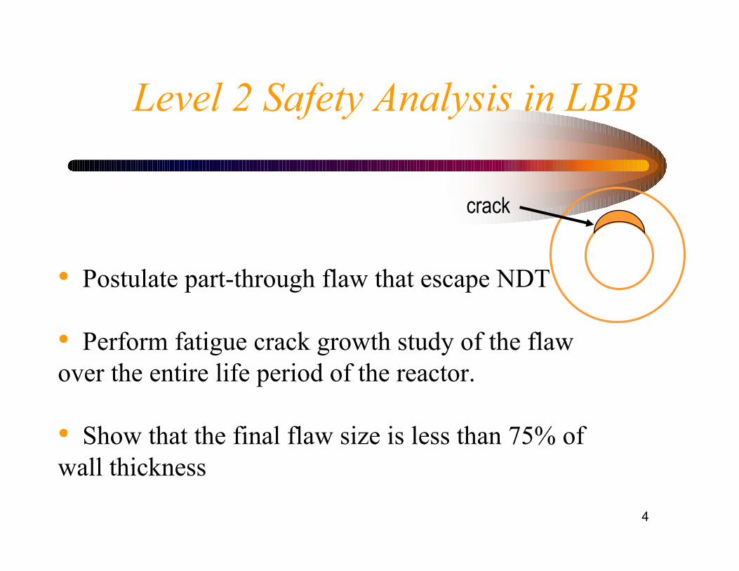
Level 2 Safety Analysis in LBB

crack

• Postulate part-through flaw that escape NDT

• Perform fatigue crack growth study of the flawover the entire life period of the reactor.

• Show that the final flaw size is less than 75% ofwall thickness

5

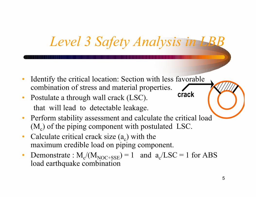
Level 3 Safety Analysis in LBB

• Identify the critical location: Section with less favorablecombination of stress and material properties.

• Postulate a through wall crack (LSC). that will lead to detectable leakage.• Perform stability assessment and calculate the critical load

(Mc) of the piping component with postulated LSC.• Calculate critical crack size (ac) with the

maximum credible load on piping component.• Demonstrate : Mc/(MNOC+SSE) = 1 and ac/LSC = 1 for ABS

load earthquake combination

crack

6

Application of LBB requires

• Knowledge of DBA loads• Geometry of the pipes• Material properties of pipe• Leakage size crack

• Some of these show variability• Requires Application of Probabilistic Fracture

MechanicsProbability that LSC is not critical under NOC+SSE

7

Salient Features of the Analysis

• Critical locations• Welds in straight pipe• Elbows, Crack at Extrados

� Steam Generator Inlet (SGI)� Steam Generator Outlet (SGO)� Pump Discharge Line (PDL)

• Critical Load: NOC + SSE

8

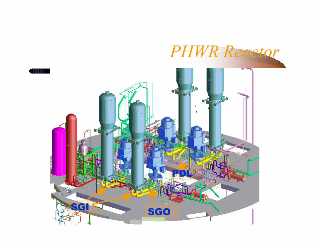
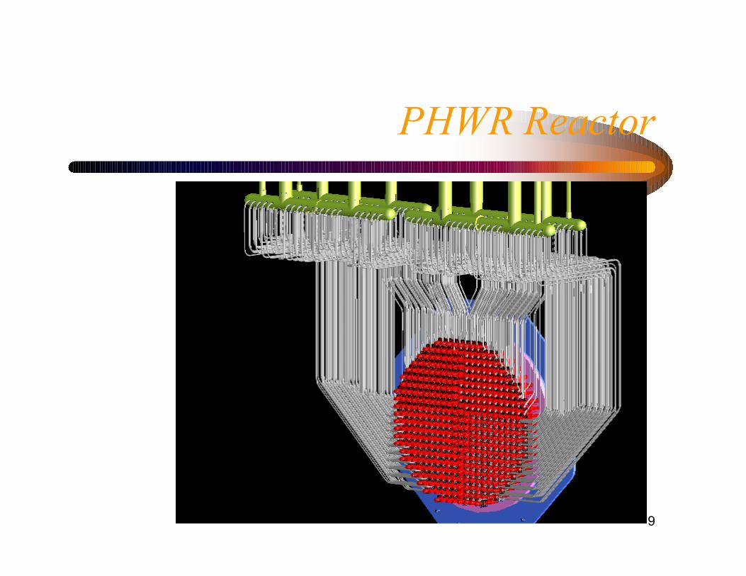
PHWR Reactor

SGI SGO

PDL

9

PHWR Reactor

10

Reliability analysis

• Data for uncertainty quantification• Material Properties

� Fracture Toughness, Fracture Resistance curve� Yield Stress, Ultimate Stress, Stress-Strain Curve

• Leakage size crack• Frequency of occurrence of SSE load

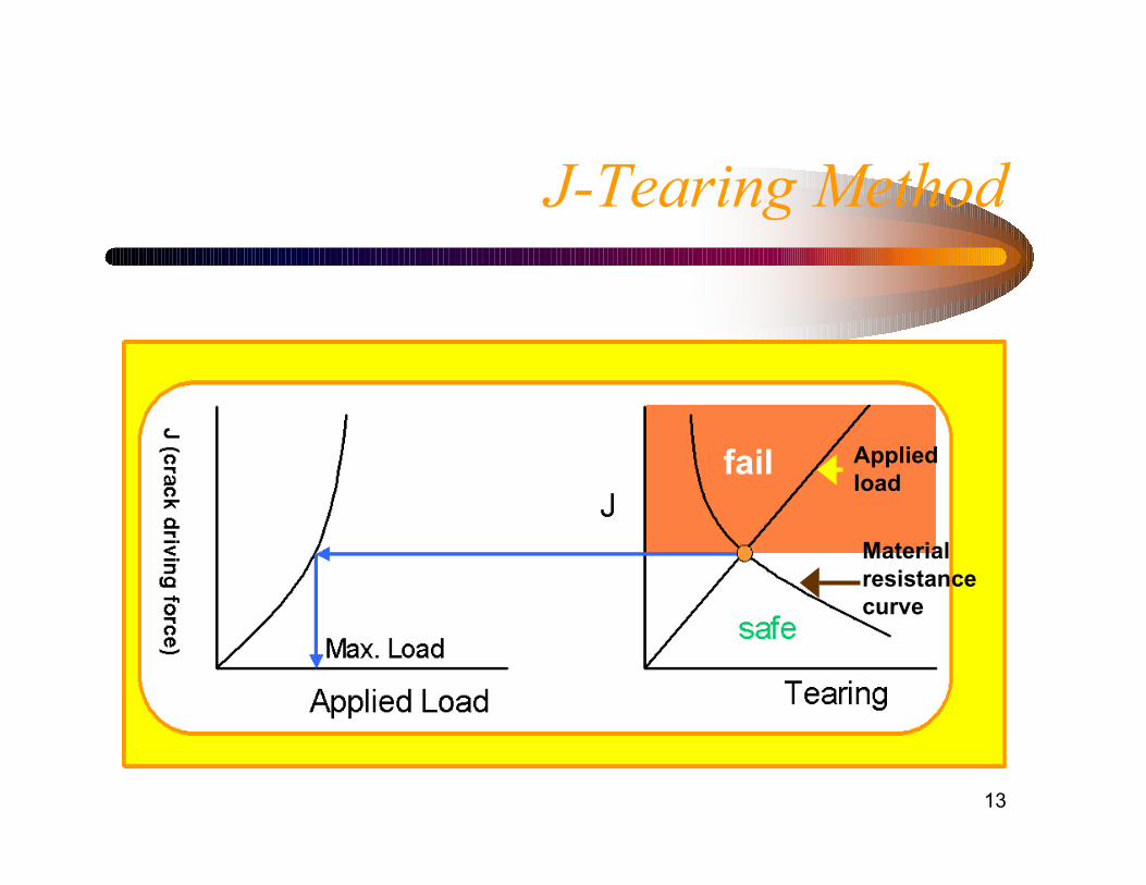
• Mechanism of failure• Net Section Collapse• J-Tearing: Crack Driving Force• R6: Failure Assessment Diagram

11

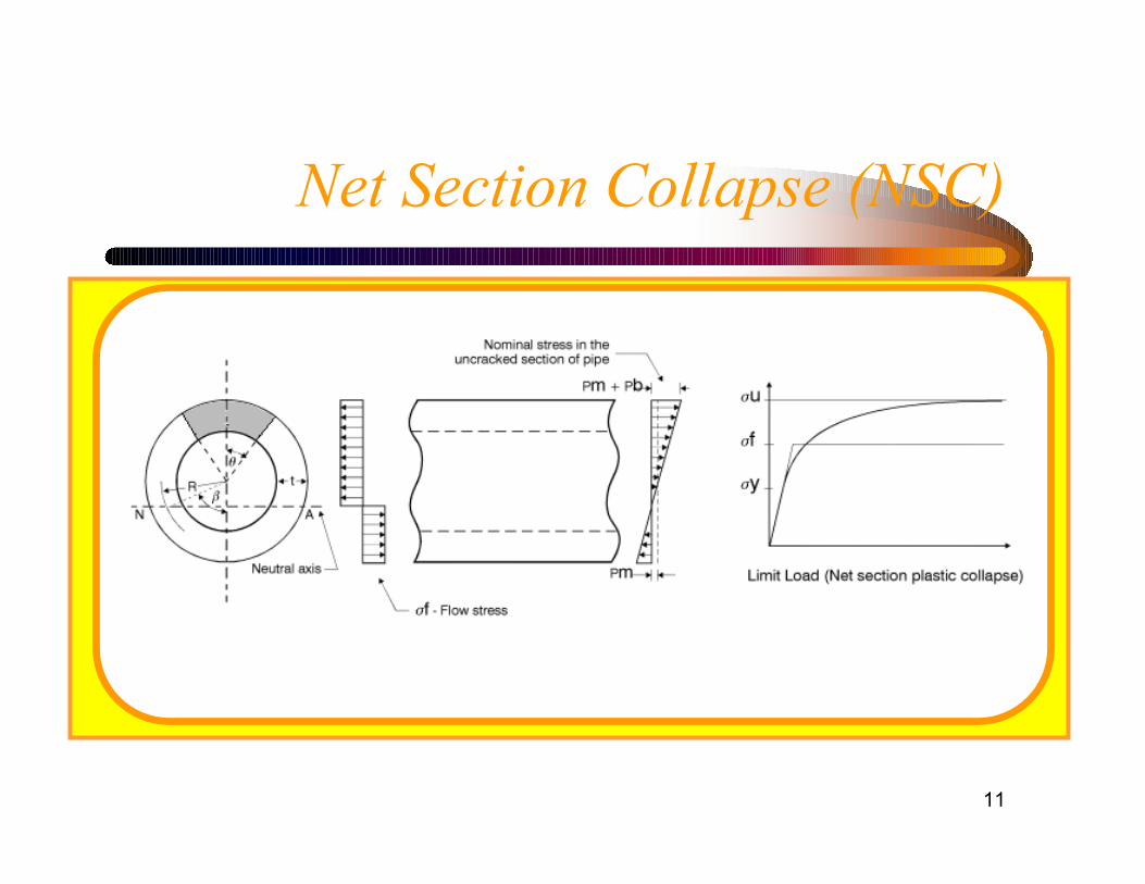
Net Section Collapse (NSC)

12

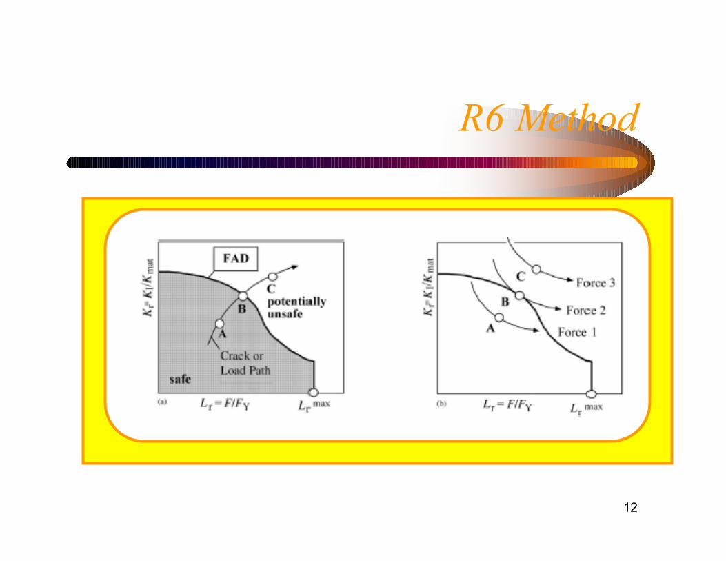
R6 Method

13

J-Tearing Method

fail Appliedload

Materialresistancecurve

14

BARC: Comprehensive ComponentIntegrity Test Program

• Fracture tests : 45 (CS) + 14 (SS)• Fatigue tests : 28 (CS) + 19 (SS)• Cyclic tearing tests : 24• Tests carried out on straight pipes and elbows at

room temperature• Sizes : 8” – 16” Nominal Bore (NB)• Tests also carried out on 100 CT specimens at RT,

200-300°C• Period of tests : 1999 - 2003

15

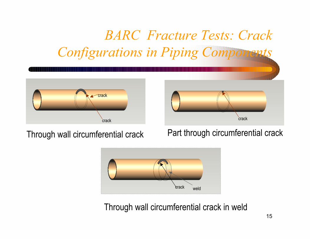
Through wall circumferential crackBARC Fracture Tests: Crack

Configurations in Piping Components

crack

crack weld

crack

crack

Through wall circumferential crack Part through circumferential crack

Through wall circumferential crack in weld

16

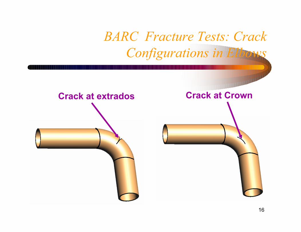
BARC Fracture Tests: CrackConfigurations in Elbows

Crack at extrados Crack at Crown

17

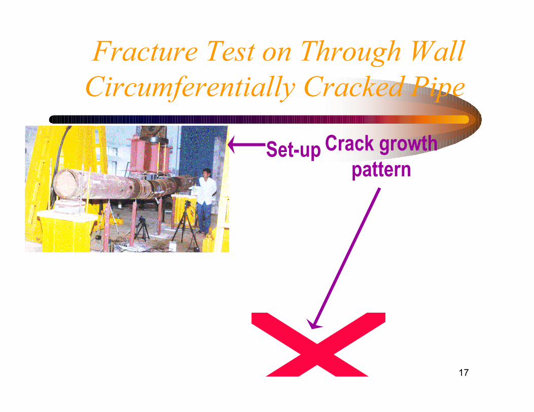
Fracture Test on Through WallCircumferentially Cracked Pipe

Set-up Crack growthpattern

18

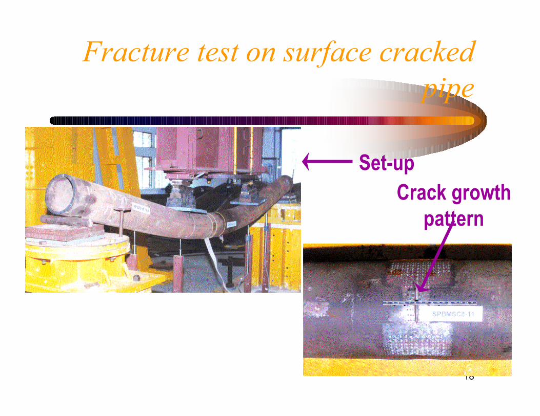
Set-upCrack growth

pattern

Fracture test on surface crackedpipe

19

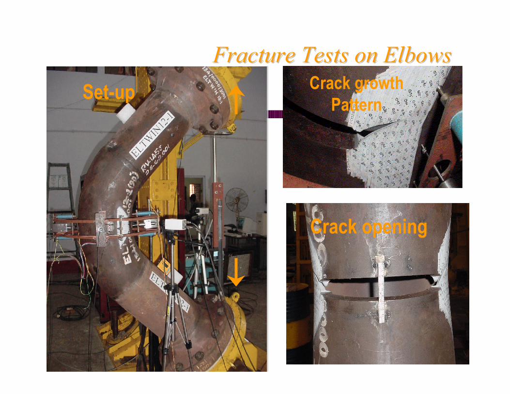
Crack growthPattern

Crack opening

Set-upFracture Tests on ElbowsFracture Tests on Elbows

20

0 40 80 120 1600

35

70

105

140

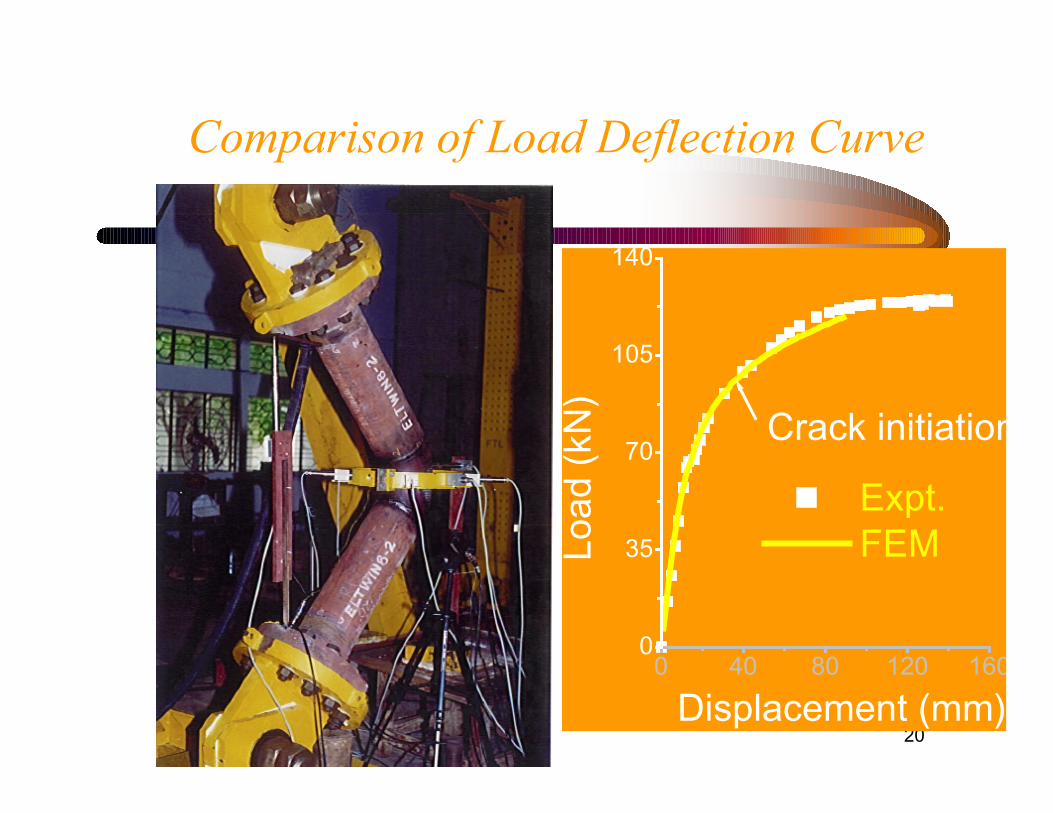
Expt. FEM

Crack initiation

Load

(kN

)

Displacement (mm)

Comparison of Load Deflection Curve

21

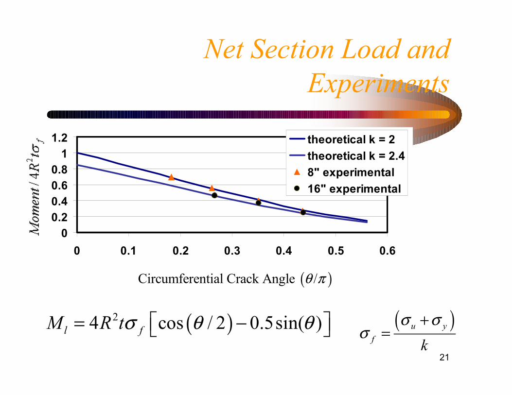
Net Section Load andExperiments

( )Circumferential Crack Angle /θ π

00.20.40.60.8

11.2

0 0.1 0.2 0.3 0.4 0.5 0.6

theoretical k = 2theoretical k = 2.48" experimental16" experimental

( )24 cos / 2 0.5sin( )l fM R tσ θ θ= −� �� � ( )u yf k

σ σσ

+=

22

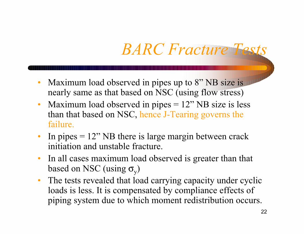
BARC Fracture Tests

• Maximum load observed in pipes up to 8” NB size isnearly same as that based on NSC (using flow stress)

• Maximum load observed in pipes = 12” NB size is lessthan that based on NSC, hence J-Tearing governs thefailure.

• In pipes = 12” NB there is large margin between crackinitiation and unstable fracture.

• In all cases maximum load observed is greater than thatbased on NSC (using σy)

• The tests revealed that load carrying capacity under cyclicloads is less. It is compensated by compliance effects ofpiping system due to which moment redistribution occurs.

23

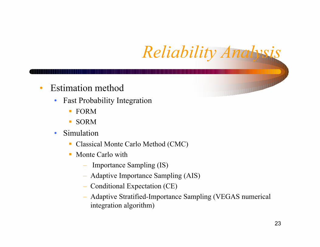
Reliability Analysis

• Estimation method• Fast Probability Integration

� FORM� SORM

• Simulation� Classical Monte Carlo Method (CMC)� Monte Carlo with

– Importance Sampling (IS)– Adaptive Importance Sampling (AIS)– Conditional Expectation (CE)– Adaptive Stratified-Importance Sampling (VEGAS numerical

integration algorithm)

24

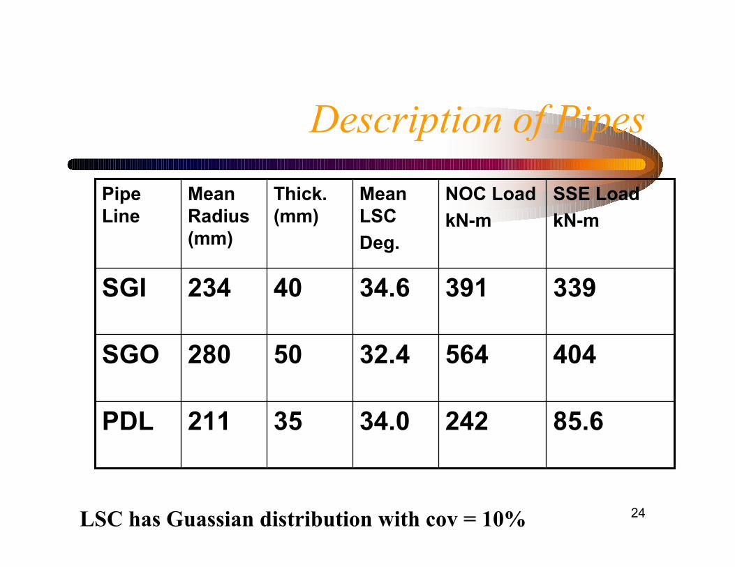
Description of Pipes

LSC has Guassian distribution with cov = 10%

85.624234.035211PDL

40456432.450280SGO

33939134.640234SGI

SSE LoadkN-m

NOC LoadkN-m

MeanLSCDeg.

Thick.(mm)

MeanRadius(mm)

PipeLine

25

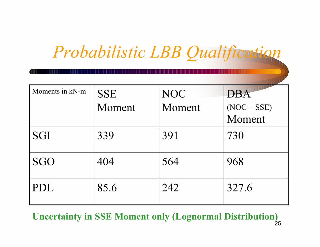
Probabilistic LBB Qualification

327.624285.6PDL

968564404SGO

730391339SGI

DBA(NOC + SSE)Moment

NOCMoment

SSEMoment

Moments in kN-m

Uncertainty in SSE Moment only (Lognormal Distribution)

26

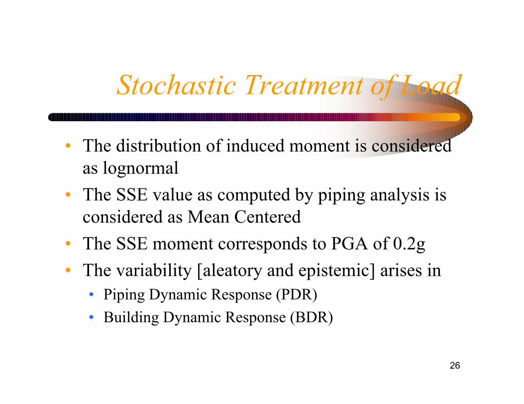
Stochastic Treatment of Load

• The distribution of induced moment is consideredas lognormal

• The SSE value as computed by piping analysis isconsidered as Mean Centered

• The SSE moment corresponds to PGA of 0.2g• The variability [aleatory and epistemic] arises in

• Piping Dynamic Response (PDR)• Building Dynamic Response (BDR)

27

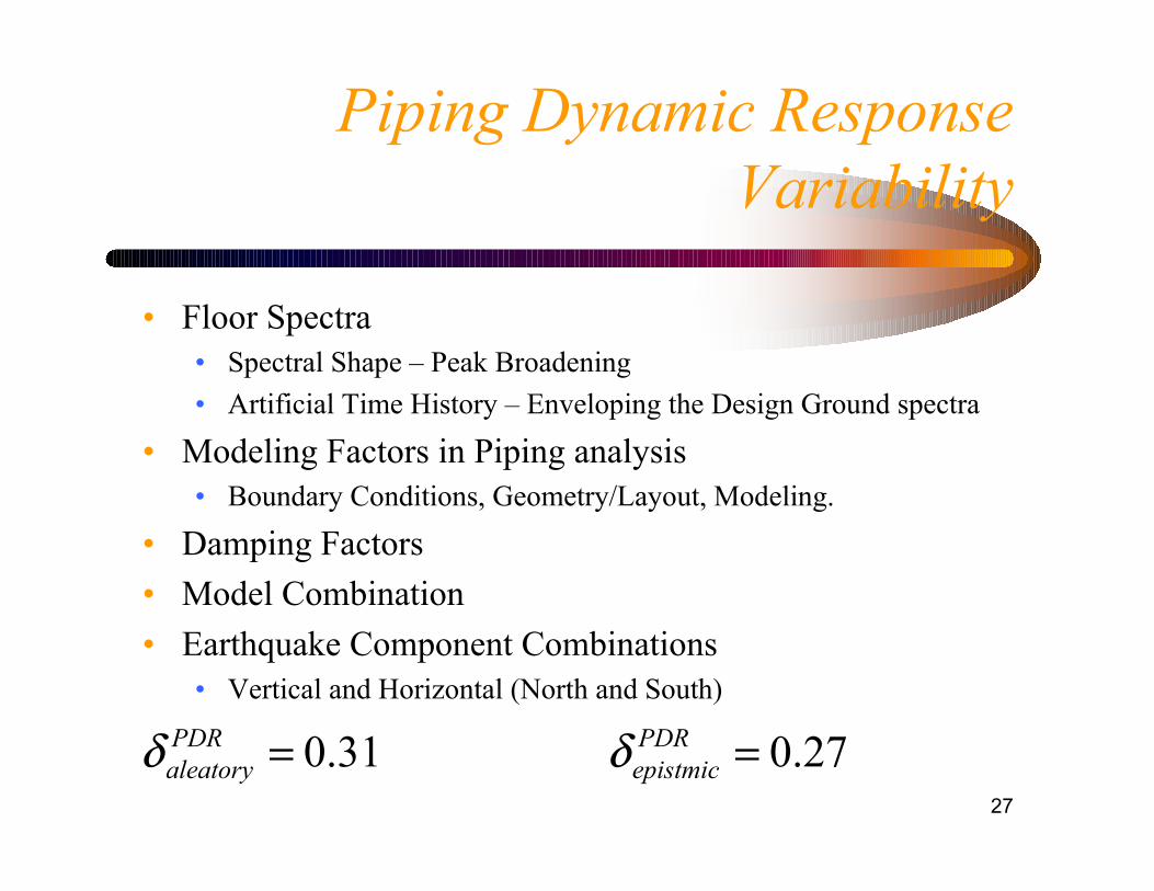
Piping Dynamic ResponseVariability

• Floor Spectra• Spectral Shape – Peak Broadening• Artificial Time History – Enveloping the Design Ground spectra

• Modeling Factors in Piping analysis• Boundary Conditions, Geometry/Layout, Modeling.

• Damping Factors• Model Combination• Earthquake Component Combinations

• Vertical and Horizontal (North and South)

0.31 0.27PDR PDRaleatory epistmic δ δ= =

28

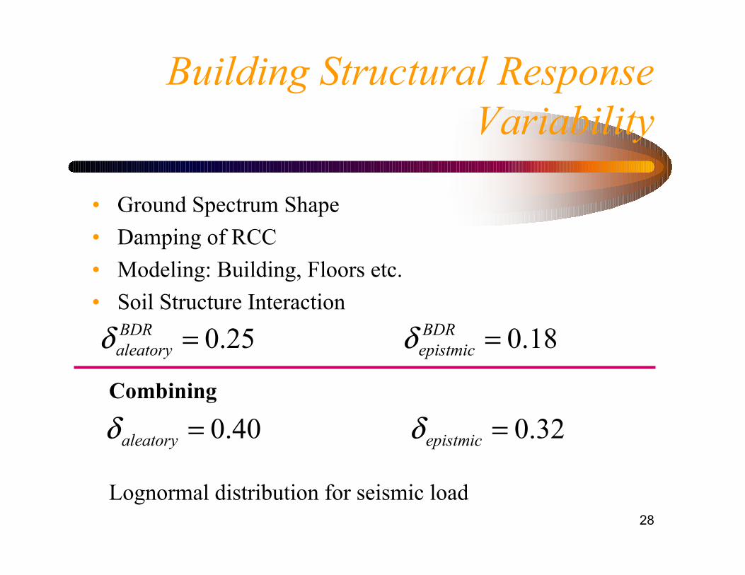
Building Structural ResponseVariability

• Ground Spectrum Shape• Damping of RCC• Modeling: Building, Floors etc.• Soil Structure Interaction

0.25 0.18BDR BDRaleatory epistmic δ δ= =

0.40 0.32aleatory epistmic δ δ= =Combining

Lognormal distribution for seismic load

29

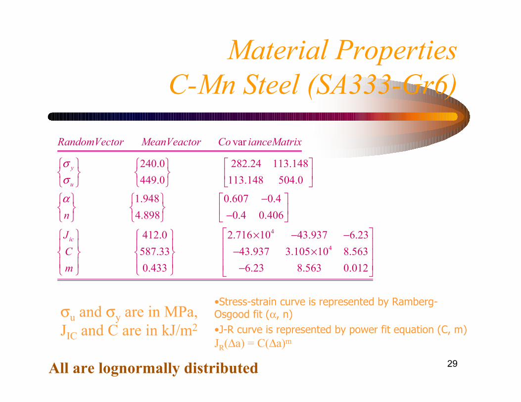
Material PropertiesC-Mn Steel (SA333-Gr6)

4

var

240.0 282.24 113.148449.0 113.148 504.0

1.948 0.607 0.44.898 0.4 0.406

412.0 2.716 10 43.93587.330.433

y

u

ic

RandomVector MeanVeactor Co ianceMatrix

n

JCm

σσα

� � � � � �� � � � � �

� �

−� � � � � �� � � � � �− � �

× −� � � � � � � �

4

7 6.2343.937 3.105 10 8.563

6.23 8.563 0.012

� �−� �− ×� �� �−� �

σu and σy are in MPa,JIC and C are in kJ/m2

•Stress-strain curve is represented by Ramberg-Osgood fit (α, n)•J-R curve is represented by power fit equation (C, m)JR(∆a) = C(∆a)m

All are lognormally distributed

30

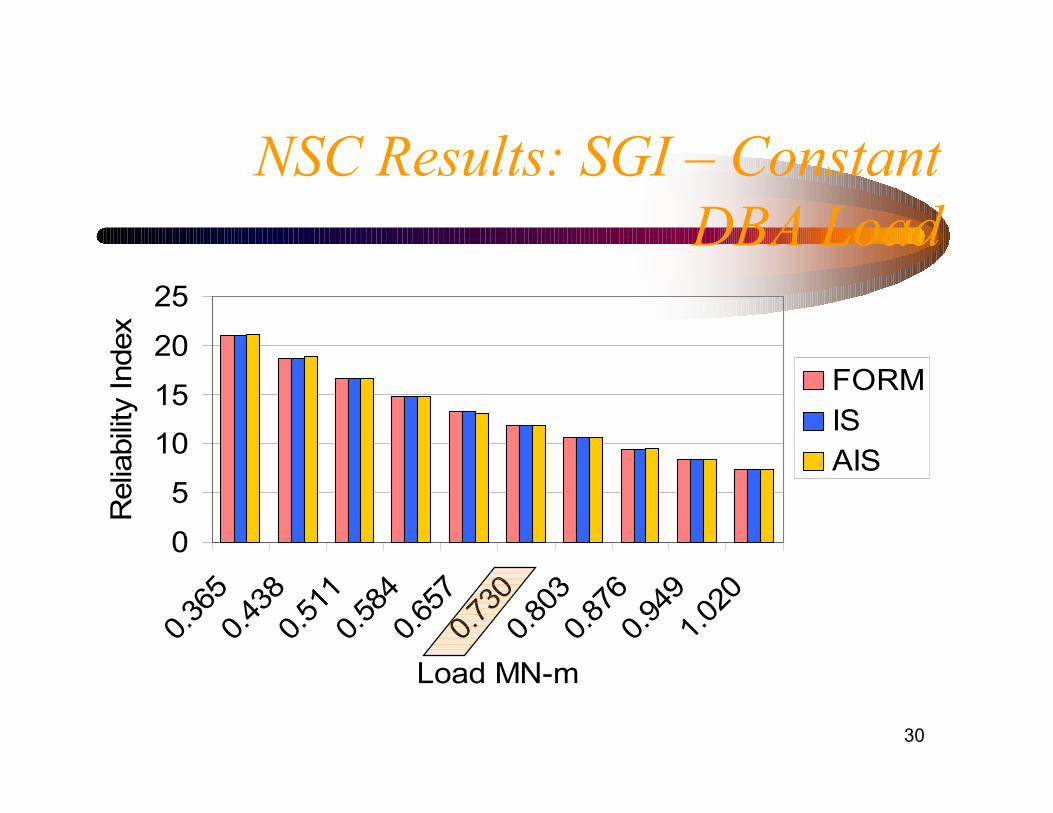
05

10152025

0.365

0.438

0.511

0.584

0.657

0.730

0.803

0.876

0.949

1.020

Load MN-m

Rel

iabi

lity

Inde

x

FORMISAIS

NSC Results: SGI – ConstantDBA Load

31

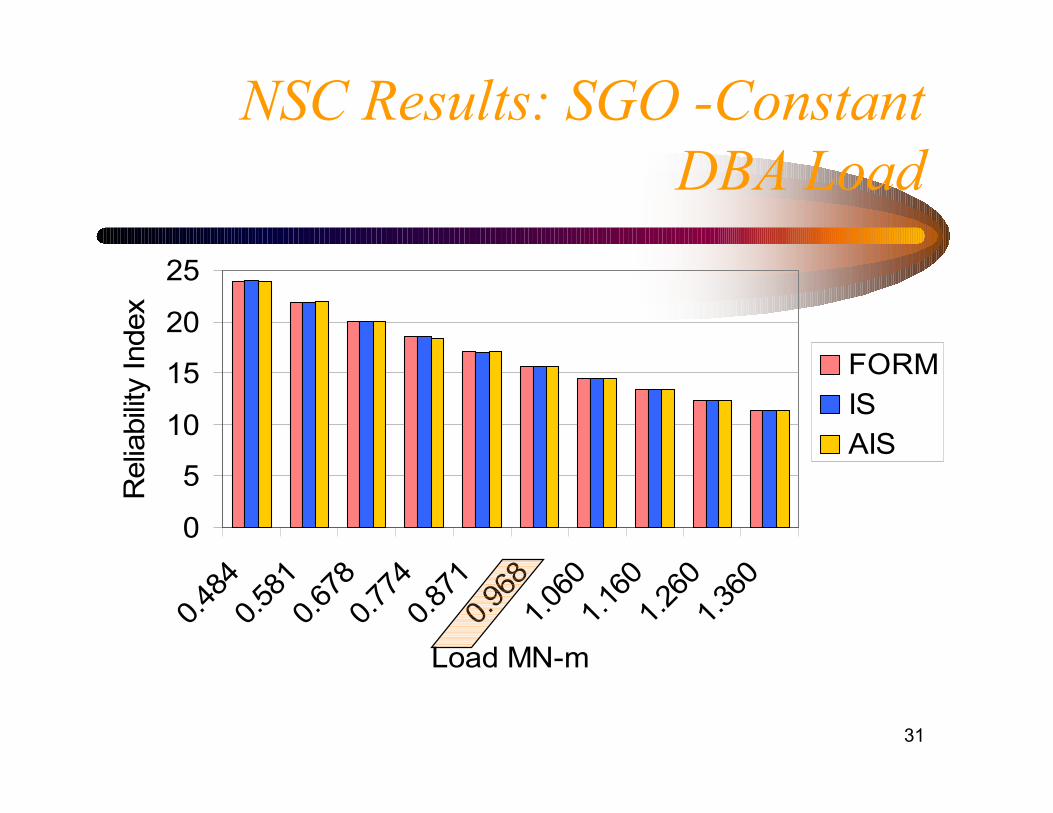
NSC Results: SGO -ConstantDBA Load

0

5

10

15

20

25

0.484

0.581

0.678

0.774

0.871

0.968

1.060

1.160

1.260

1.360

Load MN-m

Rel

iabi

lity

Inde

x

FORMISAIS

32

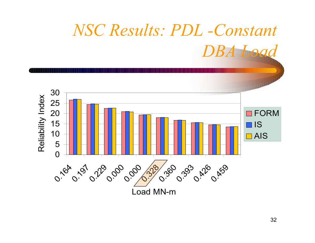
NSC Results: PDL -ConstantDBA Load

05

1015202530

0.164

0.197

0.229

0.000

0.000

0.328

0.360

0.393

0.426

0.459

Load MN-m

Rel

iabi

lity

Inde

x

FORMISAIS

33

2.00

2.50

3.00

3.50

4.00

4.50

5.00

5.50

6.00

6.50

0.365 0.438 0.511 0.584 0.657 0.73 0.803 0.876 0.949 1.02

Bending Moment (MN-m)

β

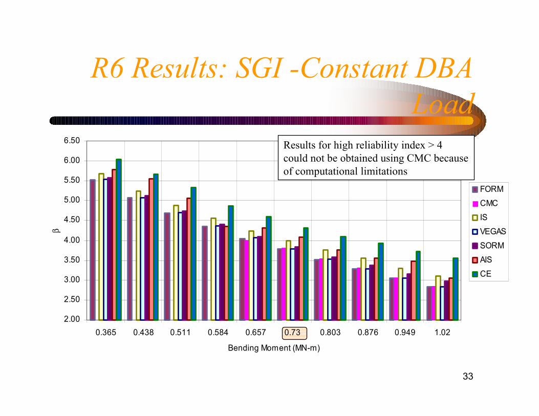
FORMCMCISVEGASSORMAISCE

R6 Results: SGI -Constant DBALoad

Results for high reliability index > 4could not be obtained using CMC becauseof computational limitations

34

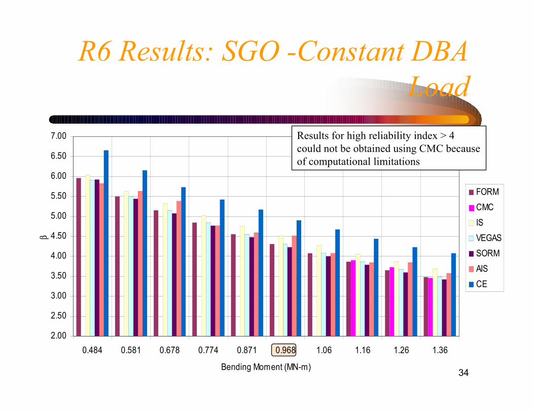
R6 Results: SGO -Constant DBALoad

2.00

2.50

3.00

3.50

4.00

4.50

5.00

5.50

6.00

6.50

7.00

0.484 0.581 0.678 0.774 0.871 0.968 1.06 1.16 1.26 1.36

Bending Moment (MN-m)

β

FORMCMCISVEGASSORMAISCE

Results for high reliability index > 4could not be obtained using CMC becauseof computational limitations

35

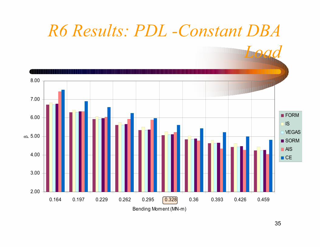
R6 Results: PDL -Constant DBALoad

2.00

3.00

4.00

5.00

6.00

7.00

8.00

0.164 0.197 0.229 0.262 0.295 0.328 0.36 0.393 0.426 0.459

Bending Moment (MN-m)

β

FORMISVEGASSORMAISCE

36

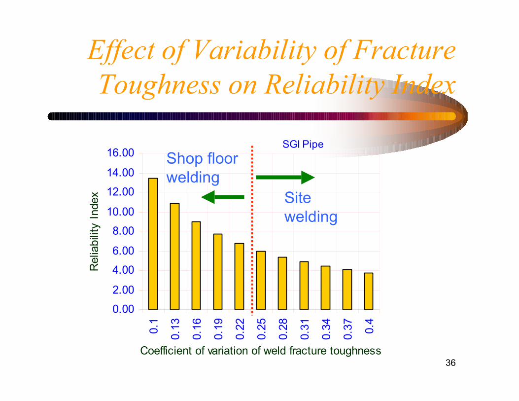
Effect of Variability of FractureToughness on Reliability Index

0.002.00

4.006.00

8.0010.00

12.0014.00

16.000.

1

0.13

0.16

0.19

0.22

0.25

0.28

0.31

0.34

0.37 0.4

Coefficient of variation of weld fracture toughness

Rel

iabi

lity

Inde

x

SGI Pipe

Sitewelding

Shop floorwelding

37

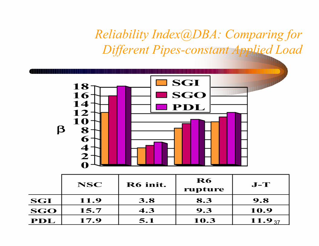
Reliability Index@DBA: Comparing forDifferent Pipes-constant Applied Load

02468

1012141618

ββββ

SGISGOPDL

SGI 11.9 3.8 8.3 9.8SGO 15.7 4.3 9.3 10.9PDL 17.9 5.1 10.3 11.9

NSC R6 init. R6 rupture J-T

38

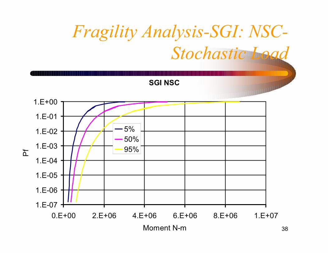
SGI NSC

1.E-07

1.E-06

1.E-05

1.E-04

1.E-03

1.E-02

1.E-01

1.E+00

0.E+00 2.E+06 4.E+06 6.E+06 8.E+06 1.E+07Moment N-m

Pf

5%50%95%

Fragility Analysis-SGI: NSC-Stochastic Load

39

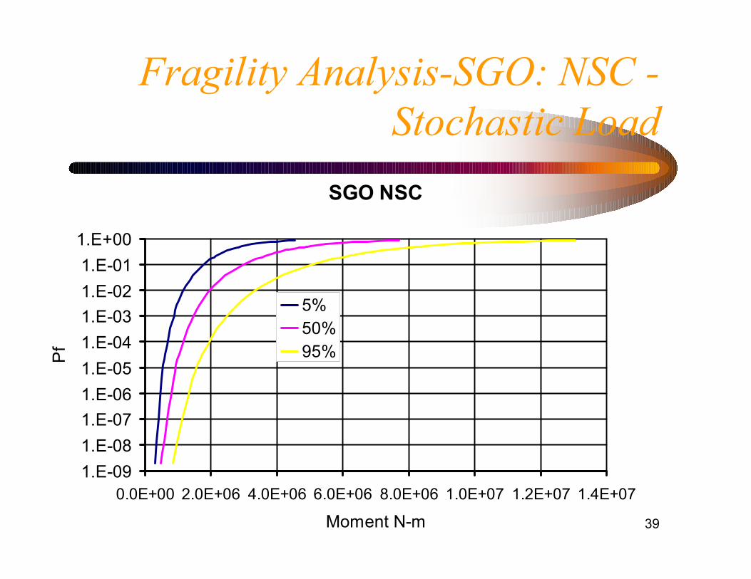
SGO NSC

1.E-091.E-081.E-071.E-061.E-051.E-041.E-031.E-021.E-01

1.E+00

0.0E+00 2.0E+06 4.0E+06 6.0E+06 8.0E+06 1.0E+07 1.2E+07 1.4E+07

Moment N-m

Pf

5%50%95%

Fragility Analysis-SGO: NSC -Stochastic Load

40

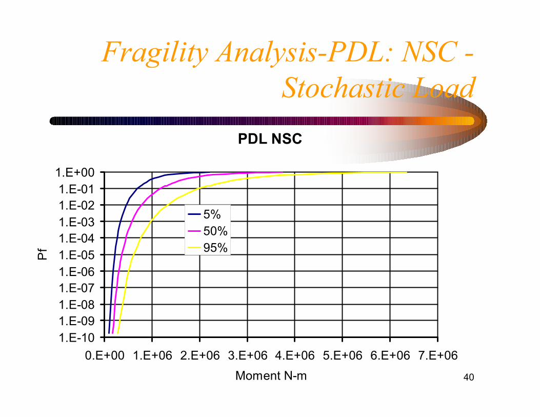
PDL NSC

1.E-101.E-091.E-081.E-071.E-061.E-051.E-041.E-031.E-021.E-01

1.E+00

0.E+00 1.E+06 2.E+06 3.E+06 4.E+06 5.E+06 6.E+06 7.E+06Moment N-m

Pf

5%50%95%

Fragility Analysis-PDL: NSC -Stochastic Load

41

SGI R6 Initiation

1.E-05

1.E-04

1.E-03

1.E-02

1.E-01

1.E+00

0.E+00 2.E+06 4.E+06 6.E+06 8.E+06Moment N-m

Pf

5%50%95%

Fragility Analysis-SGI: R6(INITIATION) - Stochastic Load

42

SGO R6 Initiation

1.E-06

1.E-05

1.E-04

1.E-03

1.E-02

1.E-01

1.E+00

0.E+00 2.E+06 4.E+06 6.E+06 8.E+06Moment N-m

Pf

5%50%95%

Fragility Analysis-SGO: R6(INITIATION) - Stochastic Load

43

PDL R6 Initiation

1.E-07

1.E-06

1.E-05

1.E-04

1.E-03

1.E-02

1.E-01

1.E+00

0.E+00 1.E+06 2.E+06 3.E+06 4.E+06 5.E+06Moment N-m

Pf

5%50%95%

Fragility Analysis-PDL: R6(INITIATION) - Stochastic Load

44

SGI R6 Max

1.E-05

1.E-04

1.E-03

1.E-02

1.E-01

1.E+00

0.E+00 2.E+06 4.E+06 6.E+06 8.E+06Moment N-m

Pf

5%50%95%

Fragility Analysis-SGI: R6 (UNSTABLECRACK GROWTH) - Stochastic Load

45

SGO R6 Max

1.E-06

1.E-05

1.E-04

1.E-03

1.E-02

1.E-01

1.E+00

0.0E+00 2.0E+06 4.0E+06 6.0E+06 8.0E+06 1.0E+07 1.2E+07 1.4E+07

Moment N-m

Pf

5%50%95%

Fragility Analysis-SGO: R6 (UNSTABLECRACK GROWTH) - Stochastic Load

46

PDL R6 Max

1.E-07

1.E-06

1.E-05

1.E-04

1.E-03

1.E-02

1.E-01

1.E+00

0.0E+00 1.0E+06 2.0E+06 3.0E+06 4.0E+06 5.0E+06 6.0E+06

Moment N-m

Pf

5%50%95%

Fragility Analysis-PDL: R6 (UNSTABLECRACK GROWTH) - Stochastic Load

47

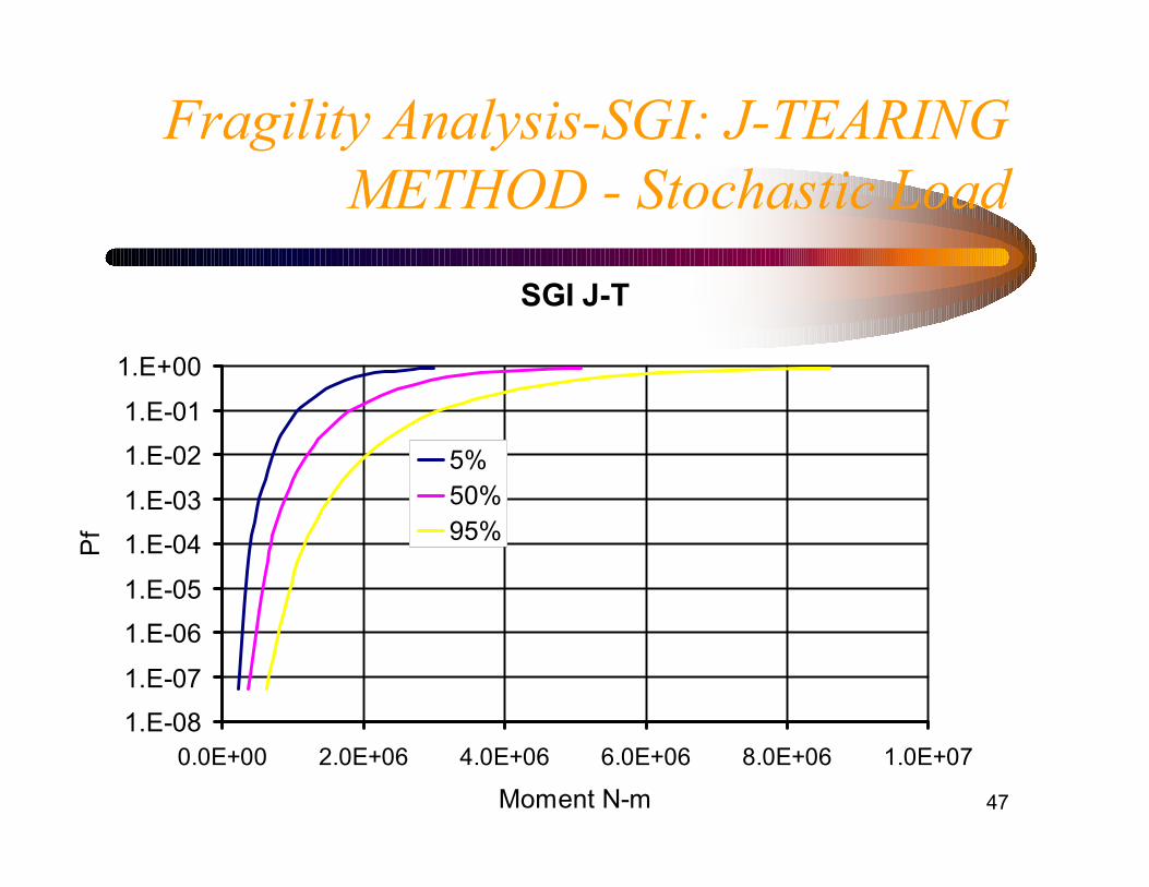
SGI J-T

1.E-081.E-07

1.E-061.E-05

1.E-041.E-03

1.E-021.E-01

1.E+00

0.0E+00 2.0E+06 4.0E+06 6.0E+06 8.0E+06 1.0E+07

Moment N-m

Pf

5%50%95%

Fragility Analysis-SGI: J-TEARINGMETHOD - Stochastic Load

48

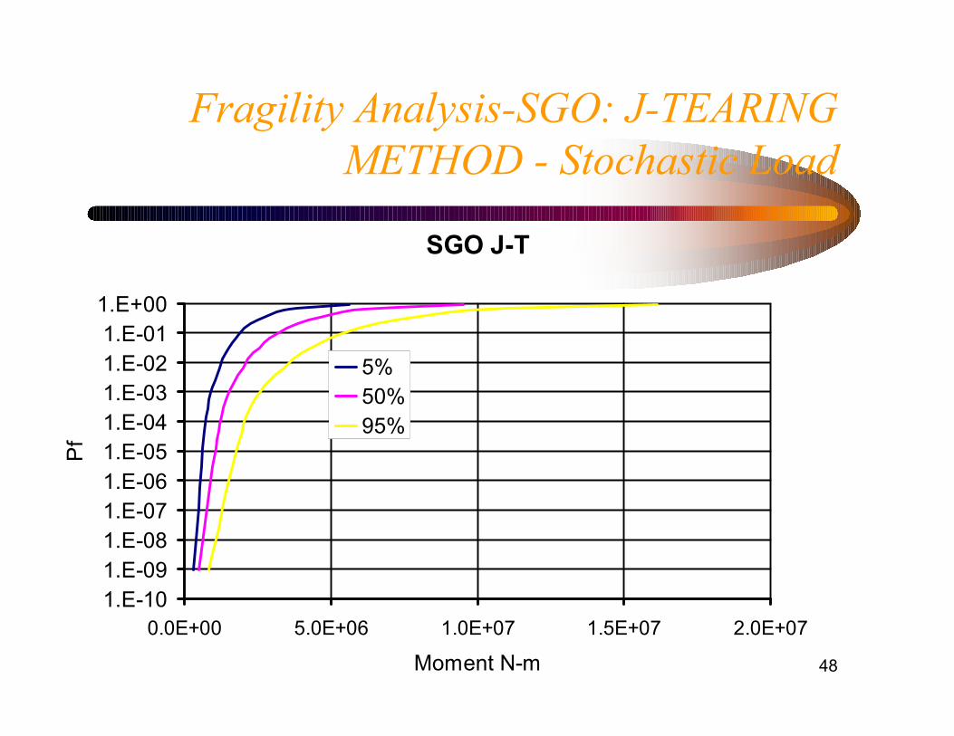
SGO J-T

1.E-101.E-091.E-081.E-071.E-061.E-051.E-041.E-031.E-021.E-01

1.E+00

0.0E+00 5.0E+06 1.0E+07 1.5E+07 2.0E+07

Moment N-m

Pf

5%50%95%

Fragility Analysis-SGO: J-TEARINGMETHOD - Stochastic Load

49

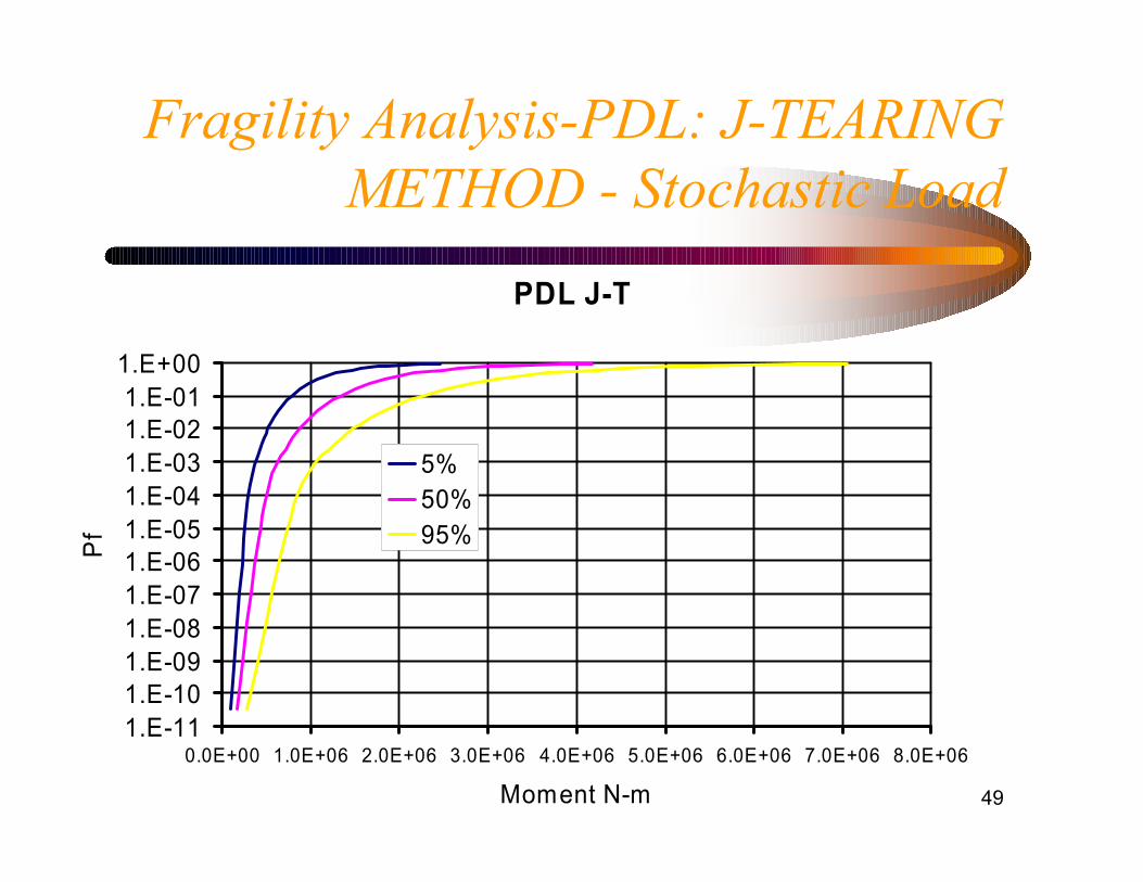
PDL J-T

1.E-111.E-101.E-091.E-081.E-071.E-061.E-051.E-041.E-031.E-021.E-01

1.E+00

0.0E+00 1.0E+06 2.0E+06 3.0E+06 4.0E+06 5.0E+06 6.0E+06 7.0E+06 8.0E+06

Moment N-m

Pf

5%50%95%

Fragility Analysis-PDL: J-TEARINGMETHOD - Stochastic Load

50

0

1

2

3

4

5R

elia

bilit

y In

dex

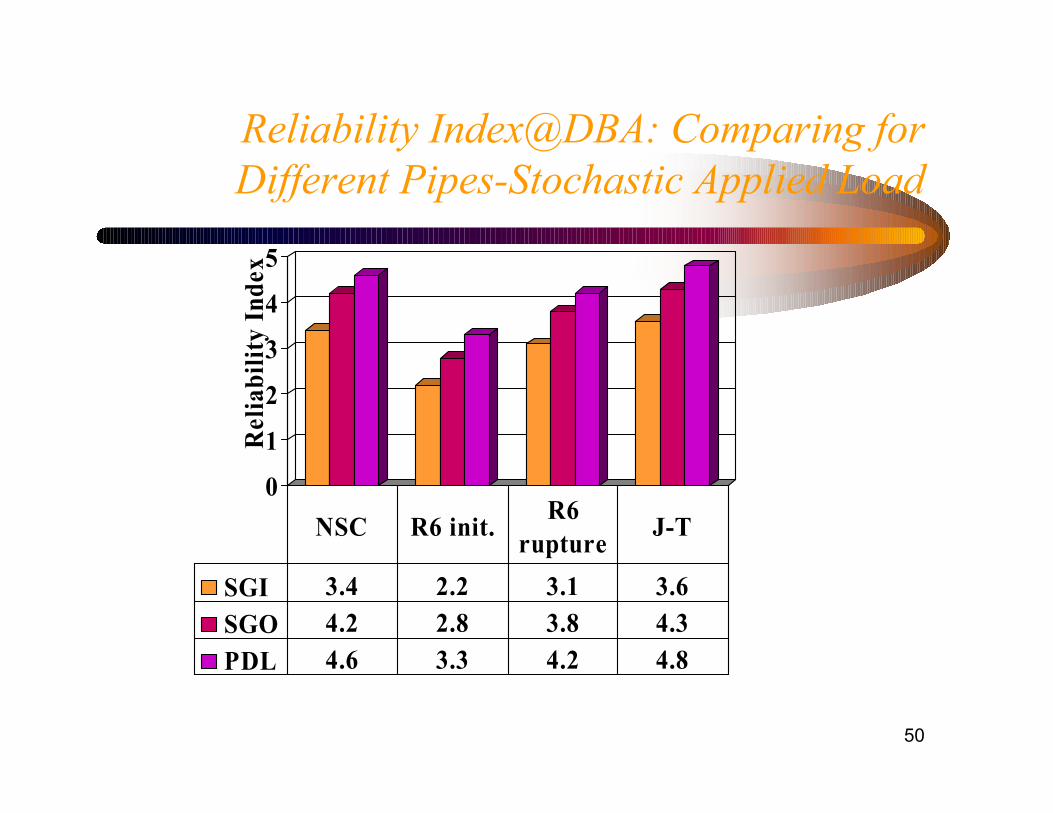
SGI 3.4 2.2 3.1 3.6SGO 4.2 2.8 3.8 4.3PDL 4.6 3.3 4.2 4.8

NSC R6 init. R6 rupture J-T

Reliability Index@DBA: Comparing forDifferent Pipes-Stochastic Applied Load

51

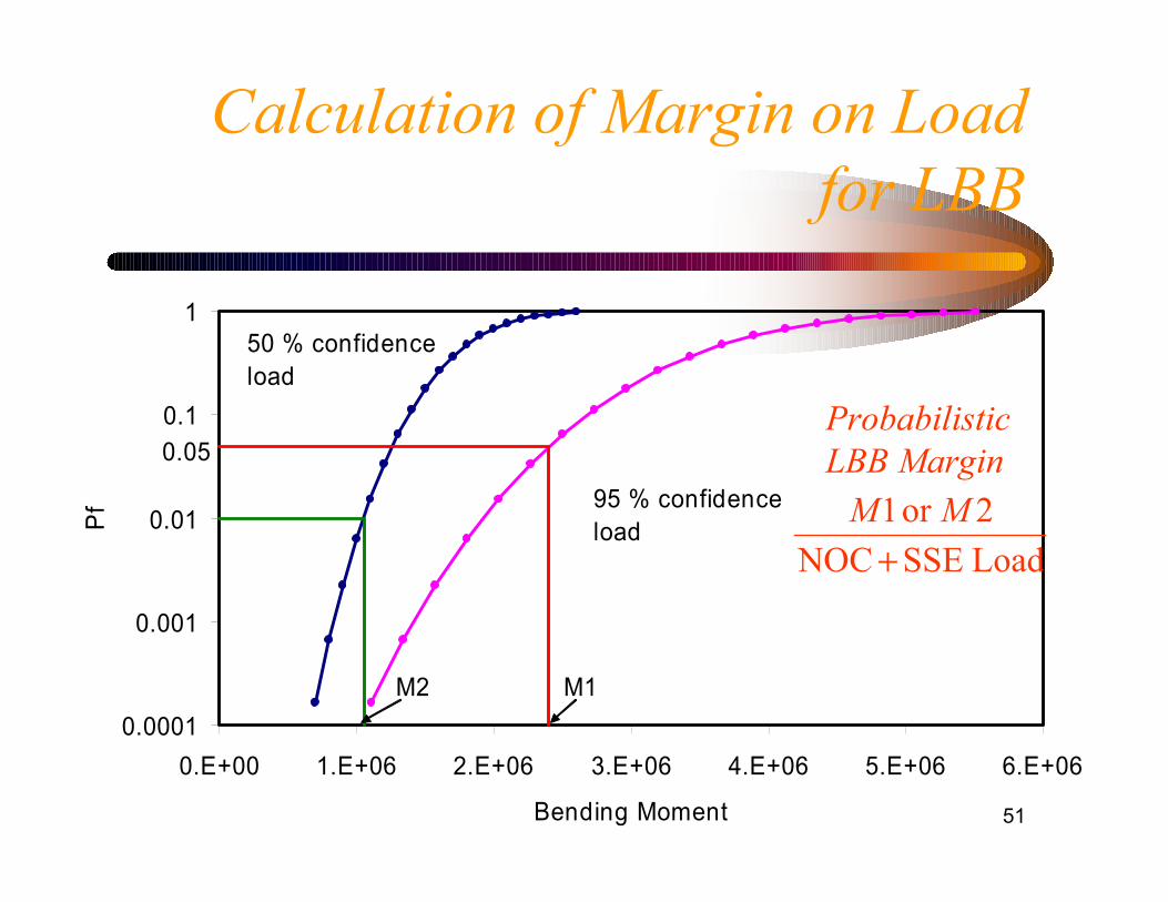
Calculation of Margin on Loadfor LBB

0.0001

0.001

0.01

0.1

1

0.E+00 1.E+06 2.E+06 3.E+06 4.E+06 5.E+06 6.E+06

Bending Moment

Pf

50 % confidence load

95 % confidence load

0.05

M1M2

LoadSSENOC2or 1

+MM

ProbabilisticLBB Margin

52

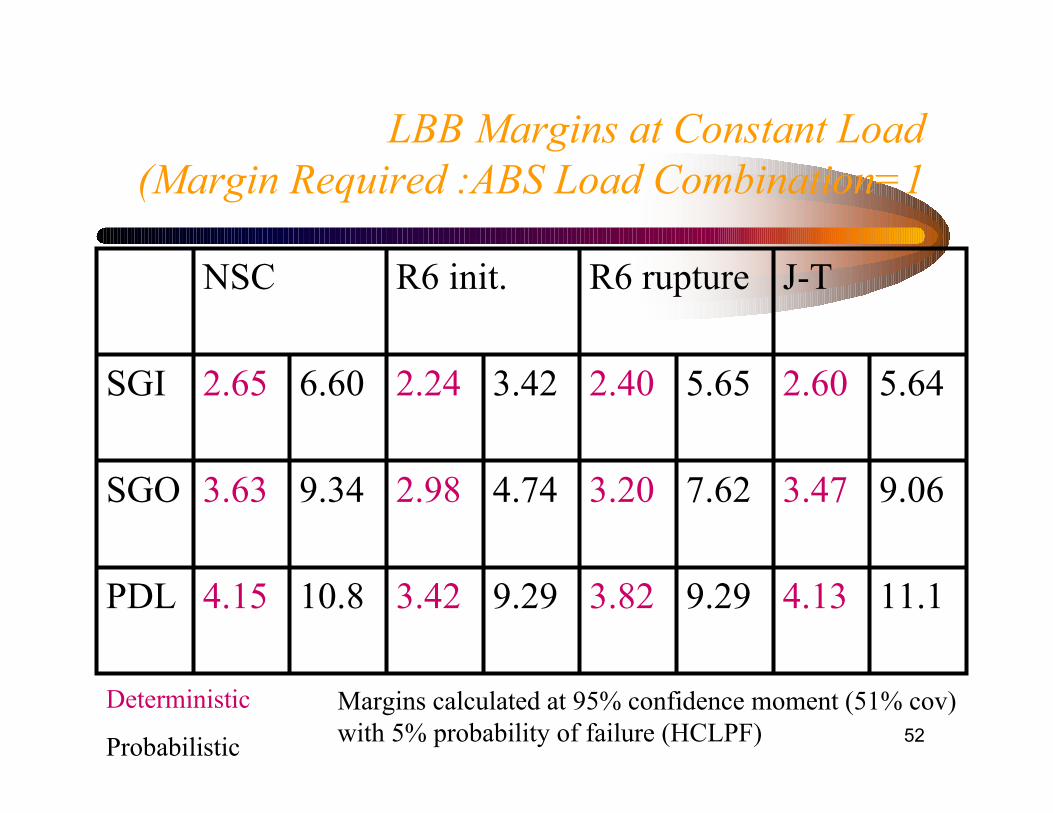
LBB Margins at Constant Load(Margin Required :ABS Load Combination=1

11.14.139.293.829.293.4210.84.15PDL

9.063.477.623.204.742.989.343.63SGO

5.642.605.652.403.422.246.602.65SGI

J-TR6 ruptureR6 init.NSC

Deterministic

Probabilistic

Margins calculated at 95% confidence moment (51% cov)with 5% probability of failure (HCLPF)

53

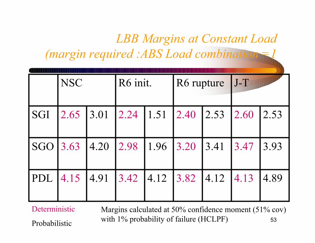
LBB Margins at Constant Load(margin required :ABS Load combination =1

4.894.134.123.824.123.424.914.15PDL

3.933.473.413.201.962.984.203.63SGO

2.532.602.532.401.512.243.012.65SGI

J-TR6 ruptureR6 init.NSC

Deterministic

Probabilistic

Margins calculated at 50% confidence moment (51% cov)with 1% probability of failure (HCLPF)

54

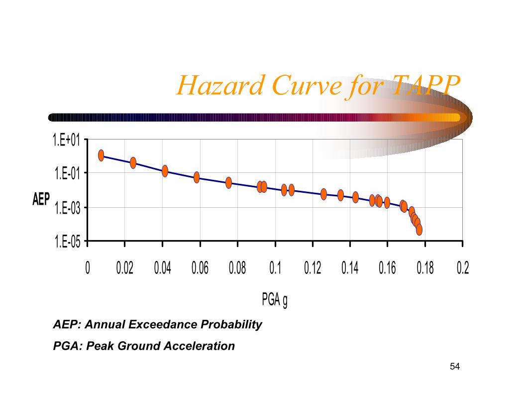
Hazard Curve for TAPP

1.E-05

1.E-03

1.E-01

1.E+01

0 0.02 0.04 0.06 0.08 0.1 0.12 0.14 0.16 0.18 0.2

PGA g

AEP

AEP: Annual Exceedance Probability

PGA: Peak Ground Acceleration

55

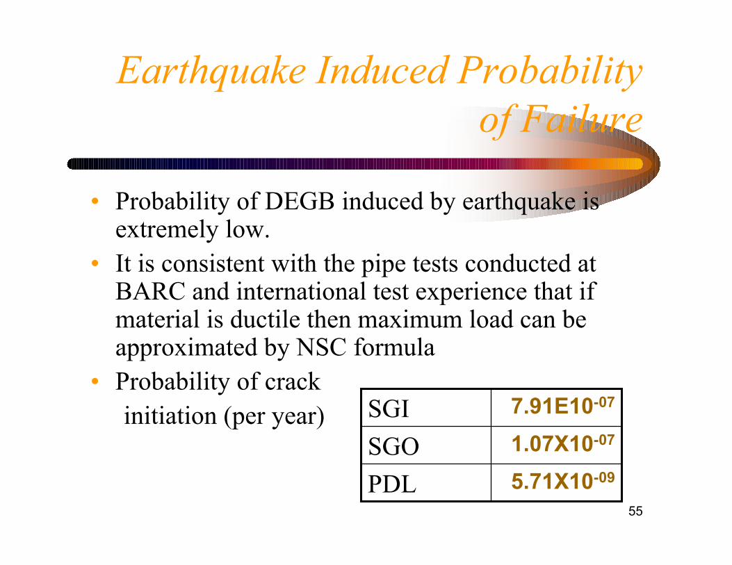
Earthquake Induced Probabilityof Failure

• Probability of DEGB induced by earthquake isextremely low.

• It is consistent with the pipe tests conducted atBARC and international test experience that ifmaterial is ductile then maximum load can beapproximated by NSC formula

• Probability of crackinitiation (per year)

5.71X10-09PDL1.07X10-07SGO7.91E10-07SGI

56

Discussion on Reliability StudiesPerformed at Constant Load

• Margins required on load for LBB qualification areobtained using probabilistic analysis

• Probability of DEGB of PHT pipe with LSC under DBAload is extremely low

• Mode of failure from experiments• Pipe sizes = 8” NB : NSC• Pipe sizes > 8” NB : J-Tearing

• Probability of stable crack growth initiation is also verylow.

• The reliability calculations were done using a number ofmethods, (FORM, SORM, Monte Carlo based etc.) All ofthem gave consistent results

57

Thank You…