Problem statement Sailco Corporation must determine how many sailboats should be produced during each of the next four quarters (one quarter = three months). The demand during each of the next four quarters is as follows: first quarter, 40 sailboats; second quarter, 60 sailboats; third quarter, 75 sailboats; fourth quarter, 25 sailboats. Sailco must meet demands on time. At the beginning of the first quarter, Sailco has an inventory of 10 sailboats. At the beginning of each quarter, Sailco must decide how many sailboats should be produced during that quarter. For simplicity, we assume that sailboats manufactured during a quarter can be used to meet demand for that quarter. During each quarter, Sailco can produce up to 40 sailboats with regular-time labour at a total cost of $400 per sailboat. By having employees work overtime during a quarter, Sailco can produce additional sailboats with overtime labor. Overtime labour is split into two categories: the total cost for the first 10 sailboats produced on overtime is $450 per sailboat; the next 10 sailboats cost $500 per sailboat. A maximum of 60 sailboats can be produced per quarter. Sailco is capable of selling each sailboat demanded during each quarter at $500 per sailboat. At the end of each quarter (after production has occurred and the current quarter’s demand has been satisfied), a carrying or holding cost of $20 per sailboat is incurred. Use i) linear programming and ii) integer programming to determine a production schedule to minimize the sum of production and inventory costs during the next four quarters. iii) Use integer programming to maximize the profit made by Sailco at the end of the fourth quarters.
Transcript
Problem statement
Sailco Corporation must determine how many sailboats should be produced during each of the next
four quarters (one quarter = three months). The demand during each of the next four quarters is as
follows: first quarter, 40 sailboats; second quarter, 60 sailboats; third quarter, 75 sailboats; fourth
quarter, 25 sailboats. Sailco must meet demands on time. At the beginning of the first quarter, Sailco
has an inventory of 10 sailboats. At the beginning of each quarter, Sailco must decide how many
sailboats should be produced during that quarter. For simplicity, we assume that sailboats
manufactured during a quarter can be used to meet demand for that quarter. During each quarter,
Sailco can produce up to 40 sailboats with regular-time labour at a total cost of $400 per sailboat. By
having employees work overtime during a quarter, Sailco can produce additional sailboats with
overtime labor. Overtime labour is split into two categories: the total cost for the first 10 sailboats
produced on overtime is $450 per sailboat; the next 10 sailboats cost $500 per sailboat. A maximum
of 60 sailboats can be produced per quarter. Sailco is capable of selling each sailboat demanded
during each quarter at $500 per sailboat.
At the end of each quarter (after production has occurred and the current quarter’s demand has
been satisfied), a carrying or holding cost of $20 per sailboat is incurred.
Use i) linear programming and ii) integer programming to determine a production schedule to
minimize the sum of production and inventory costs during the next four quarters. iii) Use integer
programming to maximize the profit made by Sailco at the end of the fourth quarters.
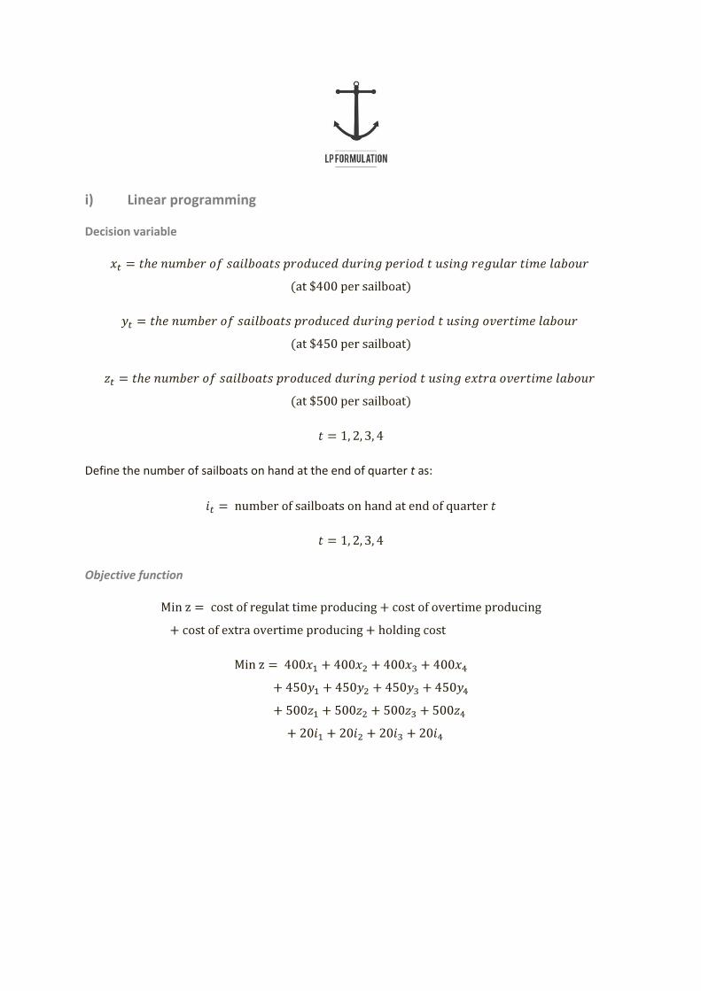
i) Linear programming
Decision variable
Define the number of sailboats on hand at the end of quarter t as:
Objective function
Subject to constraints
For quarter t:
Demand constraint:
At the end of the period these must be enough sailboats in inventory to satisfy the demand for that
period.
Capacity constraint:
A maximum of 40 sailboats can be produced using regular time labour
Only 10 sailboats can be produced using overtime labour, and only 10 sailboats can be produced
using extra overtime labour
It should be noted that the combination of the regular time constraint, the overtime constraint, and
the maximum production constraint renders the constraint for zt ≤ 10 redundant. Its presence in the
LP only serves to reduce the number iterations required to arrive at an optimal solution.
At most 60 sailboats can be produced per quarter.
Quarterly demand and inventory levels
Period (t) Inventory Demand
0 10 0
1 40
2 60
3 75
4 25
The final LP can be formulated as follows:
s.t. Demand constraint
Regular time capacity constraint
Overtime capacity constraint
Capacity constraint
Sign restriction
Sign restriction
Using any method, this LP can be solved to yield an optimal solution to minimize the cost of
production.
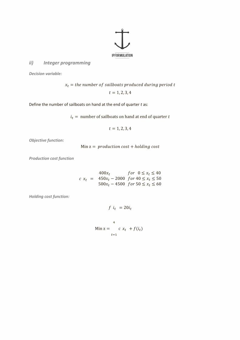
ii) Integer programming
Decision variable:
Define the number of sailboats on hand at the end of quarter t as:
Objective function:
Production cost function
Holding cost function:
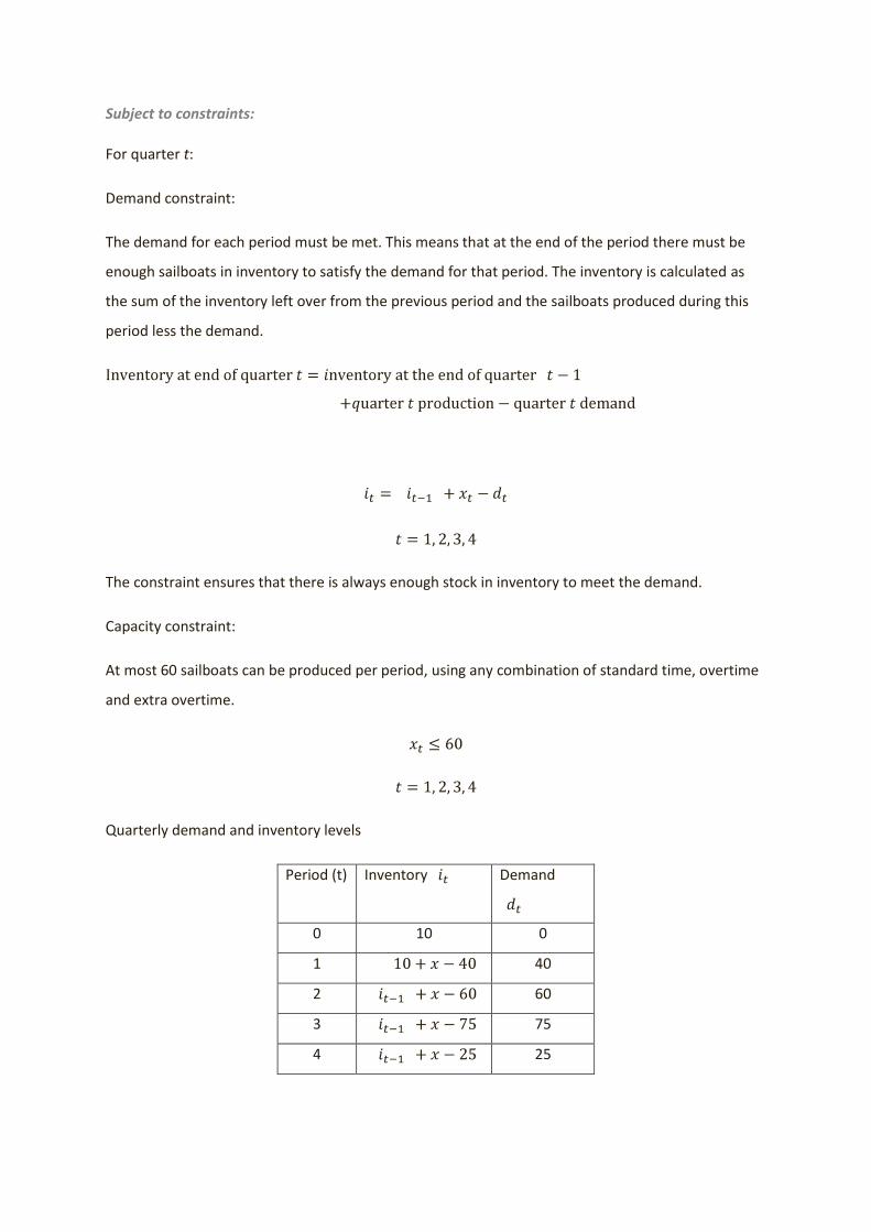
Subject to constraints:
For quarter t:
Demand constraint:
The demand for each period must be met. This means that at the end of the period there must be
enough sailboats in inventory to satisfy the demand for that period. The inventory is calculated as
the sum of the inventory left over from the previous period and the sailboats produced during this
period less the demand.
The constraint ensures that there is always enough stock in inventory to meet the demand.
Capacity constraint:
At most 60 sailboats can be produced per period, using any combination of standard time, overtime
and extra overtime.
Quarterly demand and inventory levels
Period (t) Inventory Demand
0 10 0
1 40
2 60
3 75
4 25
Formulate optimization problem:
s.t. Demand constraint for quarter t
Capacity constraint for quarter t
Sign restriction
Sign restriction
Because c(x) is a piecewise linear function, the objective function is not a linear function of x, and
this optimization problem is not an LP. By using the method described below, however, we can
transform this problem into an IP. Knowing that the break points for c(x) are 0, 40, 50, and 60, we
proceed as follows:
A piecewise linear function is not a linear function, thus general techniques used to solve linear
problems, can’t be applied. By using 0-1 variables, we are able to transform a piecewise linear
function and represent it as a linear function.
Step 1: Replace c(xt) by
Wherever c(xt) appears in the optimization problem, replace this by a new variable zti multiplied by
the cost calculated at each break point. Thus, for this problem, we find the expression above.
Step 2: Add the constraints:
The constraints listed below are a combination of 0-1 variables and the variable zti added earlier in
order to represent the piecewise linear function as a linear function.
This constraint was added in step 1. This transforms the piecewise linear function into a single, linear
function. This, however, is not sufficient in itself therefor we add the following constraints as well:
The variable yti is a binary variable (0-1 variable) which serves as a “yes-no” variable. The variable zti
is a linearization variable which ensures that the piecewise linear function can be transformed into a
linear function. These constraints will be used during the solution of the problem to decide during
which costing period (for each quarter) the sailboats will be produced.
These constraints limit the sum of all the binary variables and the sum of the linearization variables
to equal one. For the binary variables this means, for each quarter, there can only be one yti variable
equal to one. The zti variable is limited only in sign and not by value, therefor it can be any value
larger than or equal to zero (see below); however the sum of these variables for each quarter must
equal 1, which limits each variable to a fraction. This leads to the last of the linearization constraints:
These constraints have been specifically adapted to be applicable to this problem, but can be
changed for any piecewise linear problem.
This problem is made much more complex due to the fact that multiple periods are taken into the
equation. In order to formulate the problem we will initially consider only the first period.
For the first quarter, t = 1:
s.t. Demand constraint for quarter 1
Capacity constraint for quarter 1
The new formulation is the following IP:
s.t. Demand constraint for quarter 1
Capacity constraint for quarter 1
For all four quarters the IP can be written symbolically as follows:
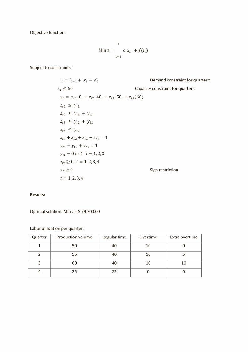
Objective function:
Subject to constraints:
Demand constraint for quarter t
Capacity constraint for quarter t
Sign restriction
Results:
Optimal solution: Min z = $ 79 700.00
Labor utilization per quarter:
Quarter Production volume Regular time Overtime Extra overtime
1 50 40 10 0
2 55 40 10 5
3 60 40 10 10
4 25 25 0 0
iii) Maximizing profit using IP
This problem statement greatly simplifies finding the maximum profit to be made by Sailco because
we can assume the only sales made are the amounts demanded each quarter. Changing the IP from
a minimisation to a maximisation problem requires only a change in the objective function as
follows:
By subtracting the cost from the sales we can determine what the maximum profit will be for this
given problem statement. The complete IP will look as follows: