Page 1
Tutorial—Evolution Strategies and Related
Estimation of Distribution Algorithms
Anne Auger & Nikolaus Hansen
INRIA Saclay - Ile-de-France, project team TAOUniversite Paris-Sud, LRI, Bat. 490
91405 ORSAY Cedex, France
Copyright is held by the author/owner(s).GECCO’08, July 12, 2008, Atlanta, Georgia, USA.ACM 978-1-60558-130-9/08/07.
Anne Auger & Nikolaus Hansen () Evolution Strategies 1 / 50
Problem Statement Black Box Optimization and Its Difficulties
Problem StatementContinuous Domain Search/Optimization
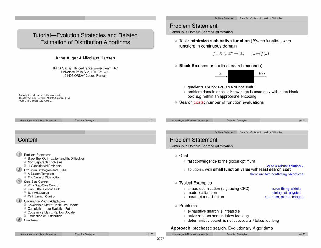
Task: minimize a objective function (fitness function, loss
function) in continuous domain
f : X ⊆ Rn → R, x 7→ f (x)
Black Box scenario (direct search scenario)
f(x)x
gradients are not available or not useful
problem domain specific knowledge is used only within the black
box, e.g. within an appropriate encoding
Search costs: number of function evaluations
Anne Auger & Nikolaus Hansen () Evolution Strategies 3 / 50
Content
1 Problem StatementBlack Box Optimization and Its DifficultiesNon-Separable ProblemsIll-Conditioned Problems
2 Evolution Strategies and EDAsA Search TemplateThe Normal Distribution
3 Step-Size ControlWhy Step-Size ControlOne-Fifth Success RuleSelf-AdaptationPath Length Control
4 Covariance Matrix AdaptationCovariance Matrix Rank-One UpdateCumulation—the Evolution PathCovariance Matrix Rank-µ UpdateEstimation of Distribution
5 Conclusion
Anne Auger & Nikolaus Hansen () Evolution Strategies 2 / 50
Problem Statement Black Box Optimization and Its Difficulties
Problem StatementContinuous Domain Search/Optimization
Goal
fast convergence to the global optimum
. . . or to a robust solution xsolution x with small function value with least search cost
there are two conflicting objectives
Typical Examples
shape optimization (e.g. using CFD) curve fitting, airfoilsmodel calibration biological, physicalparameter calibration controller, plants, images
Problems
exhaustive search is infeasible
naive random search takes too long
deterministic search is not successful / takes too long
Approach: stochastic search, Evolutionary Algorithms
Anne Auger & Nikolaus Hansen () Evolution Strategies 4 / 50
2727
ACM 978-1-60558-131-6/08/07
Page 2
Problem Statement Black Box Optimization and Its Difficulties
Metaphors
Evolutionary Computation Optimization
individual, offspring, parent ←→ candidate solution
decision variables
design variables
object variables
population ←→ set of candidate solutions
fitness function ←→ objective function
loss function
cost function
generation ←→ iteration
. . . function properties
Anne Auger & Nikolaus Hansen () Evolution Strategies 5 / 50
Problem Statement Black Box Optimization and Its Difficulties
What Makes a Function Difficult to Solve?Why stochastic search?
ruggednessnon-smooth, discontinuous, multimodal, and/or
noisy function
dimensionality
(considerably) larger than three
non-separability
dependencies between the objective variables
ill-conditioning
−4 −3 −2 −1 0 1 2 3 40
10
20
30
40
50
60
70
80
90
100
cut from 3-D example, solvablewith CMA-ES
a narrow ridge
Anne Auger & Nikolaus Hansen () Evolution Strategies 7 / 50
Problem Statement Black Box Optimization and Its Difficulties
Objective Function Properties
We assume f : X ⊂ Rn → R to have at least moderate dimensionality,
say n 6≪ 10, and to be non-linear, non-convex, and non-separable.
Additionally, f can be
multimodal
there are eventually many local optima
non-smooth
derivatives do not exist
discontinuous
ill-conditioned
noisy
. . .
Goal : cope with any of these function propertiesthey are related to real-world problems
Anne Auger & Nikolaus Hansen () Evolution Strategies 6 / 50
Problem Statement Non-Separable Problems
Separable Problems
Definition (Separable Problem)
A function f is separable if
arg min(x1,...,xn)
f (x1, . . . , xn) =
(
arg minx1
f (x1, . . .), . . . , arg minxn
f (. . . , xn)
)
⇒ it follows that f can be optimized in a sequence of n independent
1-D optimization processes
Example: Additivelydecomposable functions
f (x1, . . . , xn) =n∑
i=1
fi(xi)
Rastrigin function
−3 −2 −1 0 1 2 3−3
−2
−1
0
1
2
3
Anne Auger & Nikolaus Hansen () Evolution Strategies 8 / 50
2728
Page 3
Problem Statement Non-Separable Problems
Non-Separable ProblemsBuilding a non-separable problem from a separable one
Rotating the coordinate system
f : x 7→ f (x) separable
f : x 7→ f (Rx) non-separable
R rotation matrix
−3 −2 −1 0 1 2 3−3
−2
−1
0
1
2
3
R
−→
−3 −2 −1 0 1 2 3−3
−2
−1
0
1
2
3
12
1Hansen, Ostermeier, Gawelczyk (1995). On the adaptation of arbitrary normal mutation distributions in evolution strategies:
The generating set adaptation. Sixth ICGA, pp. 57-64, Morgan Kaufmann2
Salomon (1996). ”Reevaluating Genetic Algorithm Performance under Coordinate Rotation of Benchmark Functions; Asurvey of some theoretical and practical aspects of genetic algorithms.” BioSystems, 39(3):263-278
Anne Auger & Nikolaus Hansen () Evolution Strategies 9 / 50
Problem Statement Ill-Conditioned Problems
What Makes a Function Difficult to Solve?. . . and what can be done
The Problem What can be done
Ruggedness non-local policy, large sampling width (step-size)as large as possible while preserving a
reasonable convergence speed
stochastic, non-elitistic, population-based method
recombination operatorserves as repair mechanism
Dimensionality,
Non-Separability
exploiting the problem structurelocality, neighborhood, encoding
Ill-conditioning second order approachchanges the neighborhood metric
Anne Auger & Nikolaus Hansen () Evolution Strategies 11 / 50
Problem Statement Ill-Conditioned Problems
Ill-Conditioned Problems
If f is quadratic, f : x 7→ xTHx, ill-conditioned means a high condition number of
Hessian Matrix H
ill-conditioned means “squeezed” lines of equal function value
−1 −0.5 0 0.5 1−1
−0.8
−0.6
−0.4
−0.2
0
0.2
0.4
0.6
0.8
1
Increased
−→condition
number
−1 −0.5 0 0.5 1−1
−0.8
−0.6
−0.4
−0.2
0
0.2
0.4
0.6
0.8
1
consider the curvature of iso-fitness lines
Anne Auger & Nikolaus Hansen () Evolution Strategies 10 / 50
Evolution Strategies and EDAs
1 Problem StatementBlack Box Optimization and Its DifficultiesNon-Separable ProblemsIll-Conditioned Problems
2 Evolution Strategies and EDAsA Search TemplateThe Normal Distribution
3 Step-Size ControlWhy Step-Size ControlOne-Fifth Success RuleSelf-AdaptationPath Length Control
4 Covariance Matrix AdaptationCovariance Matrix Rank-One UpdateCumulation—the Evolution PathCovariance Matrix Rank-µ UpdateEstimation of Distribution
5 Conclusion
Anne Auger & Nikolaus Hansen () Evolution Strategies 12 / 50
2729
Page 4
Evolution Strategies and EDAs A Search Template
Stochastic Search
A black box search template to minimize f : Rn → R
Initialize distribution parameters θ, set population size λ ∈ N
While not terminate
1 Sample distribution P (x|θ)→ x1, . . . , xλ ∈ Rn
2 Evaluate x1, . . . , xλ on f
3 Update parameters θ ← Fθ(θ, x1, . . . , xλ, f (x1), . . . , f (xλ))
Everything depends on the definition of P and Fθ
deterministic algorithms are covered as well
In Evolutionary Algorithms the distribution P is often implicitly defined
via operators on a population, in particular, selection, recombination
and mutation
Natural template for Estimation of Distribution AlgorithmsAnne Auger & Nikolaus Hansen () Evolution Strategies 13 / 50
Evolution Strategies and EDAs The Normal Distribution
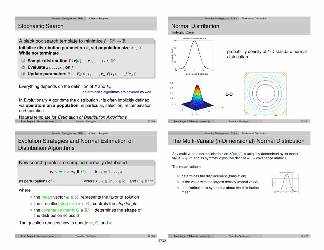
Normal DistributionIsotropic Case
−4 −2 0 2 40
0.1
0.2
0.3
0.4Standard Normal Distribution
pro
babili
ty d
ensity
probability density of 1-D standard normal
distribution
−5
0
5
−5
0
50
0.1
0.2
0.3
0.4
2−D Normal Distribution
2-D
−1 −0.5 0 0.5 1−1
−0.8
−0.6
−0.4
−0.2
0
0.2
0.4
0.6
0.8
1
Anne Auger & Nikolaus Hansen () Evolution Strategies 15 / 50
Evolution Strategies and EDAs A Search Template
Evolution Strategies and Normal Estimation of
Distribution Algorithms
New search points are sampled normally distributed
xi ∼ m + σNi(0, C) for i = 1, . . . , λ
as perturbations of m where xi, m ∈ Rn, σ ∈ R+, and C ∈ R
n×n
where
the mean vector m ∈ Rn represents the favorite solution
the so-called step-size σ ∈ R+ controls the step length
the covariance matrix C ∈ Rn×n determines the shape of
the distribution ellipsoid
The question remains how to update m, C, and σ.
Anne Auger & Nikolaus Hansen () Evolution Strategies 14 / 50
Evolution Strategies and EDAs The Normal Distribution
The Multi-Variate (n-Dimensional) Normal Distribution
Any multi-variate normal distribution N (m, C) is uniquely determined by its mean
value m ∈ Rn and its symmetric positive definite n× n covariance matrix C.
The mean value m
determines the displacement (translation)
is the value with the largest density (modal value)
the distribution is symmetric about the distribution
mean −4 −2 0 2 40
0.1
0.2
0.3
0.4Standard Normal Distribution
pro
ba
bili
ty d
en
sity
Anne Auger & Nikolaus Hansen () Evolution Strategies 16 / 50
2730
Page 5
Evolution Strategies and EDAs The Normal Distribution
The covariance matrix C determines the shape. It has a valuable geometrical
interpretation: any covariance matrix can be uniquely identified with the iso-density
ellipsoid {x ∈ Rn | xT
C−1x = 1}
Lines of Equal Density
N`m, σ2
I´∼ m + σN (0, I)
one degree of freedom σcomponents of N (0, I)are independent standard
normally distributed
N`m, D
2´∼ m + DN (0, I)
n degrees of freedom
components are
independent, scaled
N (m, C)∼ m + C12N (0, I)
(n2 + n)/2 degrees of freedom
components are
correlated
. . . CMA
Anne Auger & Nikolaus Hansen () Evolution Strategies 17 / 50
Evolution Strategies and EDAs The Normal Distribution
The (µ/µ, λ)-ESNon-elitist selection and intermediate (weighted) recombination
Given the i-th solution point xi = m + σ Ni(0, C)︸ ︷︷ ︸
=: yi
= m + σ yi
Let xi:λ the i-th ranked solution point, such that f (x1:λ) ≤ · · · ≤ f (xλ:λ).
The new mean reads
m←µ
∑
i=1
wi xi:λ = m + σ
µ∑
i=1
wi yi:λ
︸ ︷︷ ︸
=: yw
where
w1 ≥ · · · ≥ wµ > 0,∑µ
i=1 wi = 1
The best µ points are selected from the new solutions (non-elitistic)
and weighted intermediate recombination is applied.
Anne Auger & Nikolaus Hansen () Evolution Strategies 19 / 50
Evolution Strategies and EDAs The Normal Distribution
Evolution Strategies
(µ +, λ) µ: # parents, λ: # offspring
+ selection in {parents} ∪ {offspring}, selection in {offspring}
(1 + 1)-ES
Sample one offspring from parent m
x = m + σN (0, C)
If x better than m select
m← x
. . . why?
Anne Auger & Nikolaus Hansen () Evolution Strategies 18 / 50
Step-Size Control Why Step-Size Control
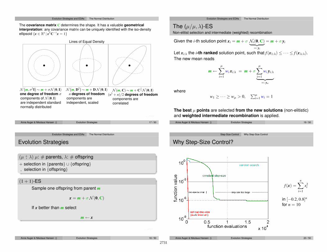
Why Step-Size Control?
f (x) =n∑
i=1
x2i
in [−0.2, 0.8]n
for n = 10
Anne Auger & Nikolaus Hansen () Evolution Strategies 20 / 50
2731
Page 6
Step-Size Control Why Step-Size Control
Why Step-Size Control?
f (x) =n∑
i=1
x2i
in [−0.2, 0.8]n
for n = 10
Anne Auger & Nikolaus Hansen () Evolution Strategies 21 / 50
Step-Size Control Why Step-Size Control
Why Step-Size Control?
f (x) =n∑
i=1
x2i
in [−0.2, 0.8]n
for n = 10
Anne Auger & Nikolaus Hansen () Evolution Strategies 23 / 50
Step-Size Control Why Step-Size Control
Why Step-Size Control?
f (x) =n∑
i=1
x2i
in [−0.2, 0.8]n
for n = 10
Anne Auger & Nikolaus Hansen () Evolution Strategies 22 / 50
Step-Size Control Why Step-Size Control
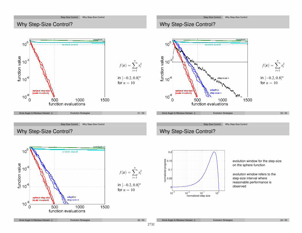
Why Step-Size Control?
10−3
10−2
10−1
100
0
0.05
0.1
0.15
0.2
no
rma
lize
d p
rog
ress
normalized step size
evolution window for the step-size
on the sphere function
evolution window refers to the
step-size interval where
reasonable performance is
observed
Anne Auger & Nikolaus Hansen () Evolution Strategies 24 / 50
2732
Page 7
Step-Size Control Why Step-Size Control
Methods for Step-Size Control
1/5-th success ruleab, often applied with “+”-selection
increase step-size if more than 20% of the new solutions are successful,
decrease otherwise
σ-self-adaptationc, applied with “,”-selection
mutation is applied to the step-size and the better one, according to the
objective function value, is selected
simplified “global” self-adaptation
path length controld (Cumulative Step-size Adaptation, CSA)e, applied with
“,”-selection
aRechenberg 1973, Evolutionsstrategie, Optimierung technischer Systeme nach Prinzipien der biologischen Evolution,
Frommann-Holzboogb
Schumer and Steiglitz 1968. Adaptive step size random search. IEEE TACc
Schwefel 1981, Numerical Optimization of Computer Models, Wileyd
Hansen & Ostermeier 2001, Completely Derandomized Self-Adaptation in Evolution Strategies, Evol. Comput. 9(2)e
Ostermeier et al 1994, Step-size adaptation based on non-local use of selection information, PPSN IVAnne Auger & Nikolaus Hansen () Evolution Strategies 25 / 50
Step-Size Control One-Fifth Success Rule
One-fifth success rule
������������������������������������������������������������������������������������������������������������������������������������������������������������������������������������������������������������������������������������������������������������������������������������������������������������������������������������������������������������������������������������������������������������������������������������������������������������������������������������������������������������������������������������������������������������������������������������������������������������������������������������������������������������������������������������������������������������������������������������������������������������������������������������������������������������������������������������������������������������������������������������������������������������������������������������������������������������������������������������������������������������������������������������������������������������������������������������������������������������������������������������������������������������������������������������������������������������������������������������������������������������������������������������������������������������������������������������������������������������������������������������������������������������������������������������������������������������������������������������������������������������������������������
������������������������������������������������������������������������������������������������������������������������������������������������������������������������������������������������������������������������������������������������������������������������������������������������������������������������������������������������������������������������������������������������������������������������������������������������������������������������������������������������������������������������������������������������������������������������������������������������������������������������������������������������������������������������������������������������������������������������������������������������������������������������������������������������������������������������������������������������������������������������������������������������������������������������������������������������������������������������������������������������������������������������������������������������������������������������������������������������������������������������������������������������������������������������������������������������������������������������������������������������������������������������������������������������������������������������������������������������������������������������������������������������������������������������������������������������������������������������������������������������������������������������������
���������������������������������������������������������������������������������������������������������������������������������������������������������������������������������������������������������������������������������������
���������������������������������������������������������������������������������������������������������������������������������������������������������������������������������������������������������������������������������������
Proba of success (ps)
1/2 1/5
Proba of success (ps)
“too small”
Anne Auger & Nikolaus Hansen () Evolution Strategies 27 / 50
Step-Size Control One-Fifth Success Rule
One-fifth success rule
������������������������������������������������������������������������������������������������������������������������������������������������������������������������������������������������������������������������������������������������������������������������������������������������������������������������������������������������������������������������������������������������������������������������������������������������������������������������������������������������������������������������������������������������������������������������������������������������������������������������������������������������������������������������������������������������������������������������������������������������������������������������������������������������������������������������������������������������������������������������������������������������������������������������������������������������������������������������������������������������������������������������������������������������������������������������������������������������������������������������������������������������������������������������������������������������������������������������������������������������������������������������������������������������������������������������������������������������������������������������������������������������������������������������������������������������������������������������������������������������������������������������������
������������������������������������������������������������������������������������������������������������������������������������������������������������������������������������������������������������������������������������������������������������������������������������������������������������������������������������������������������������������������������������������������������������������������������������������������������������������������������������������������������������������������������������������������������������������������������������������������������������������������������������������������������������������������������������������������������������������������������������������������������������������������������������������������������������������������������������������������������������������������������������������������������������������������������������������������������������������������������������������������������������������������������������������������������������������������������������������������������������������������������������������������������������������������������������������������������������������������������������������������������������������������������������������������������������������������������������������������������������������������������������������������������������������������������������������������������������������������������������������������������������������������������
���������������������������������������������������������������������������������������������������������������������������������������������������������������������������������������������������������������������������������������
���������������������������������������������������������������������������������������������������������������������������������������������������������������������������������������������������������������������������������������
↓increase σ
↓decrease σ
Anne Auger & Nikolaus Hansen () Evolution Strategies 26 / 50
Step-Size Control One-Fifth Success Rule
One-fifth success rule
Let ps: # of successful offspring / generation
σ ← σ × exp
(1
3× ps − ptarget
1− ptarget
)
Increase σ if ps > ptarget
Decrease σ if ps < ptarget
(1 + 1)-ES
ptarget = 1/5
IF offspring better parent
ps = 1
ELSE
ps = 0
Anne Auger & Nikolaus Hansen () Evolution Strategies 28 / 50
2733
Page 8
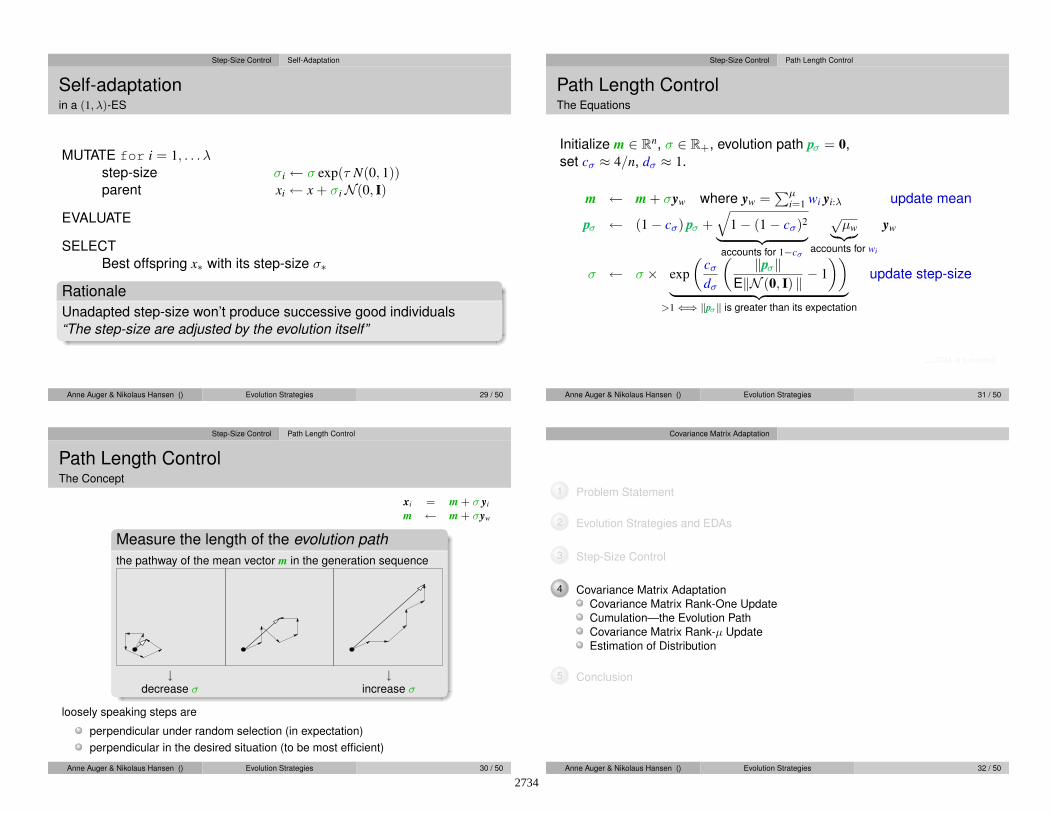
Step-Size Control Self-Adaptation
Self-adaptationin a (1, λ)-ES
MUTATE for i = 1, . . . λstep-size σi ← σ exp(τ N(0, 1))parent xi ← x + σiN(0, I)
EVALUATE
SELECT
Best offspring x∗ with its step-size σ∗
Rationale
Unadapted step-size won’t produce successive good individuals
“The step-size are adjusted by the evolution itself”
Anne Auger & Nikolaus Hansen () Evolution Strategies 29 / 50
Step-Size Control Path Length Control
Path Length ControlThe Equations
Initialize m ∈ Rn, σ ∈ R+, evolution path pσ = 0,
set cσ ≈ 4/n, dσ ≈ 1.
m ← m + σyw where yw =∑µ
i=1 wi yi:λ update mean
pσ ← (1− cσ) pσ +√
1− (1− cσ)2
︸ ︷︷ ︸
accounts for 1−cσ
õw
︸︷︷︸
accounts for wi
yw
σ ← σ × exp
(cσ
dσ
( ‖pσ‖E‖N (0, I) ‖ − 1
))
︸ ︷︷ ︸
>1⇐⇒ ‖pσ‖ is greater than its expectation
update step-size
. . . CMA in a nutshell
Anne Auger & Nikolaus Hansen () Evolution Strategies 31 / 50
Step-Size Control Path Length Control
Path Length ControlThe Concept
xi = m + σ yi
m ← m + σyw
Measure the length of the evolution path
the pathway of the mean vector m in the generation sequence
↓decrease σ
↓increase σ
loosely speaking steps are
perpendicular under random selection (in expectation)
perpendicular in the desired situation (to be most efficient)
Anne Auger & Nikolaus Hansen () Evolution Strategies 30 / 50
Covariance Matrix Adaptation
1 Problem Statement
2 Evolution Strategies and EDAs
3 Step-Size Control
4 Covariance Matrix Adaptation
Covariance Matrix Rank-One Update
Cumulation—the Evolution Path
Covariance Matrix Rank-µ Update
Estimation of Distribution
5 Conclusion
Anne Auger & Nikolaus Hansen () Evolution Strategies 32 / 50
2734
Page 9
Covariance Matrix Adaptation Covariance Matrix Rank-One Update
Covariance Matrix AdaptationRank-One Update
m ← m + σyw, yw =∑µ
i=1 wi yi:λ, yi ∼ Ni(0, C)
new distribution,
C← 0.8× C + 0.2× ywyTw
the ruling principle: the adaptation increases the probability of success-
ful steps, yw, to appear again
. . . equations
Anne Auger & Nikolaus Hansen () Evolution Strategies 33 / 50
Covariance Matrix Adaptation Covariance Matrix Rank-One Update
C← (1− ccov)C + ccovµwywyTw
covariance matrix adaptation
learns all pairwise dependencies between variablesoff-diagonal entries in the covariance matrix reflect the dependencies
conducts a principle component analysis (PCA) of steps yw,
sequentially in time and spaceeigenvectors of the covariance matrix C are the principle components / the
principle axes of the mutation ellipsoid
learns a new, rotated problem represen-
tation and a new metric (Mahalanobis)components are independent (only) in the new representation
approximates the inverse Hessian on quadratic functions
overwhelming empirical evidence, proof is in progress
. . . cumulation, rank-µ, step-size control
Anne Auger & Nikolaus Hansen () Evolution Strategies 35 / 50
Covariance Matrix Adaptation Covariance Matrix Rank-One Update
Covariance Matrix AdaptationRank-One Update
Initialize m ∈ Rn, and C = I, set σ = 1, learning rate ccov ≈ 2/n2
While not terminate
xi = m + σ yi, yi ∼ Ni(0, C) ,
m ← m + σyw where yw =
µ∑
i=1
wi yi:λ
C ← (1− ccov)C + ccovµw ywyTw
︸︷︷︸
rank-one
where µw =1
∑µi=1 wi
2≥ 1
Anne Auger & Nikolaus Hansen () Evolution Strategies 34 / 50
Covariance Matrix Adaptation Covariance Matrix Rank-One Update
1 Problem Statement
2 Evolution Strategies and EDAs
3 Step-Size Control
4 Covariance Matrix Adaptation
Covariance Matrix Rank-One Update
Cumulation—the Evolution Path
Covariance Matrix Rank-µ Update
Estimation of Distribution
5 Conclusion
Anne Auger & Nikolaus Hansen () Evolution Strategies 36 / 50
2735
Page 10
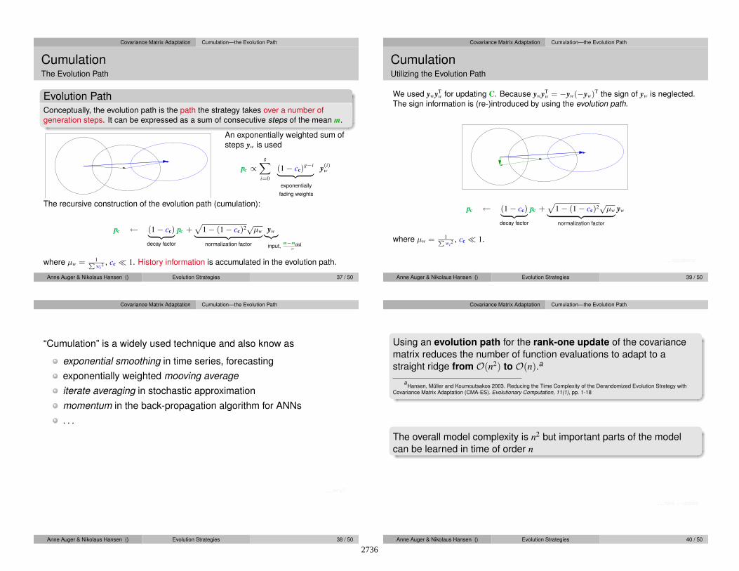
Covariance Matrix Adaptation Cumulation—the Evolution Path
CumulationThe Evolution Path
Evolution Path
Conceptually, the evolution path is the path the strategy takes over a number of
generation steps. It can be expressed as a sum of consecutive steps of the mean m.
An exponentially weighted sum of
steps yw is used
pc ∝gX
i=0
(1− cc)g−i
| {z }
exponentially
fading weights
y(i)w
The recursive construction of the evolution path (cumulation):
pc ← (1− cc)| {z }
decay factor
pc +p
1− (1− cc)2√
µw| {z }
normalization factor
yw|{z}
input,m−mold
σ
where µw = 1P
wi2 , cc ≪ 1. History information is accumulated in the evolution path.
Anne Auger & Nikolaus Hansen () Evolution Strategies 37 / 50
Covariance Matrix Adaptation Cumulation—the Evolution Path
CumulationUtilizing the Evolution Path
We used ywyTw for updating C. Because ywyT
w = −yw(−yw)T the sign of yw is neglected.
The sign information is (re-)introduced by using the evolution path.
pc ← (1− cc)| {z }
decay factor
pc +p
1− (1− cc)2√
µw| {z }
normalization factor
yw
where µw = 1P
wi2 , cc ≪ 1.
. . . equations
Anne Auger & Nikolaus Hansen () Evolution Strategies 39 / 50
Covariance Matrix Adaptation Cumulation—the Evolution Path
“Cumulation” is a widely used technique and also know as
exponential smoothing in time series, forecasting
exponentially weighted mooving average
iterate averaging in stochastic approximation
momentum in the back-propagation algorithm for ANNs
. . .
. . . why?
Anne Auger & Nikolaus Hansen () Evolution Strategies 38 / 50
Covariance Matrix Adaptation Cumulation—the Evolution Path
Using an evolution path for the rank-one update of the covariance
matrix reduces the number of function evaluations to adapt to a
straight ridge from O(n2) to O(n).a
aHansen, Muller and Koumoutsakos 2003. Reducing the Time Complexity of the Derandomized Evolution Strategy with
Covariance Matrix Adaptation (CMA-ES). Evolutionary Computation, 11(1), pp. 1-18
The overall model complexity is n2 but important parts of the model
can be learned in time of order n
. . . rank µ update
Anne Auger & Nikolaus Hansen () Evolution Strategies 40 / 50
2736
Page 11
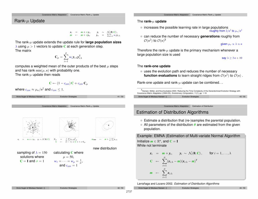
Covariance Matrix Adaptation Covariance Matrix Rank-µ Update
Rank-µ Update
xi = m + σ yi, yi ∼ Ni(0, C) ,
m ← m + σyw yw =Pµ
i=1wi yi:λ
The rank-µ update extends the update rule for large population sizes
λ using µ > 1 vectors to update C at each generation step.
The matrix
Cµ =
µ∑
i=1
wi yi:λyTi:λ
computes a weighted mean of the outer products of the best µ steps
and has rank min(µ, n) with probability one.
The rank-µ update then reads
C← (1− ccov) C + ccov Cµ
where ccov ≈ µw/n2 and ccov ≤ 1.
Anne Auger & Nikolaus Hansen () Evolution Strategies 41 / 50
Covariance Matrix Adaptation Covariance Matrix Rank-µ Update
The rank-µ update
increases the possible learning rate in large populationsroughly from 2/n2 to µw/n2
can reduce the number of necessary generations roughly from
O(n2) to O(n)3
given µw ∝ λ ∝ n
Therefore the rank-µ update is the primary mechanism whenever a
large population size is usedsay λ ≥ 3 n + 10
The rank-one update
uses the evolution path and reduces the number of necessary
function evaluations to learn straight ridges from O(n2) to O(n) .
Rank-one update and rank-µ update can be combined. . .
3Hansen, Muller, and Koumoutsakos 2003. Reducing the Time Complexity of the Derandomized Evolution Strategy with
Covariance Matrix Adaptation (CMA-ES). Evolutionary Computation, 11(1), pp. 1-18
Anne Auger & Nikolaus Hansen () Evolution Strategies 43 / 50
Covariance Matrix Adaptation Covariance Matrix Rank-µ Update
xi = m + σ yi, yi ∼ N (0, C)
sampling of λ = 150
solutions where
C = I and σ = 1
Cµ = 1µ
P
yi:λyTi:λ
C ← (1− 1)× C + 1× Cµ
calculating C where
µ = 50,
w1 = · · · = wµ = 1µ
,
and ccov = 1
mnew ← m + 1µ
P
yi:λ
new distribution
Anne Auger & Nikolaus Hansen () Evolution Strategies 42 / 50
Covariance Matrix Adaptation Estimation of Distribution
Estimation of Distribution Algorithms
Estimate a distribution that (re-)samples the parental population.
All parameters of the distribution θ are estimated from the given
population.
Example: EMNA (Estimation of Multi-variate Normal Algorithm
Initialize m ∈ Rn, and C = I
While not terminate
xi = m + yi, yi ∼ Ni(0, C) , for i = 1, . . . , λ
C ←µ
∑
i=1
(xi:λ −m)(xi:λ −m)T
m ←µ
∑
i=1
xi:λ
Larranaga and Lozano 2002. Estimation of Distribution Algorithms
Anne Auger & Nikolaus Hansen () Evolution Strategies 44 / 50
2737
Page 12
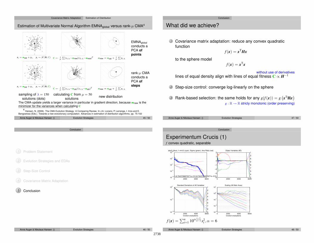
Covariance Matrix Adaptation Estimation of Distribution
Estimation of Multivariate Normal Algorithm EMNAglobal versus rank-µ CMA4
xi = mold + yi, yi ∼ N (0, C)
xi = mold + yi, yi ∼ N (0, C)
sampling of λ = 150
solutions (dots)
C← 1µ
P
(xi:λ−mnew)(xi:λ−mnew)T
C← 1µ
P
(xi:λ−mold)(xi:λ−mold)T
calculating C from µ = 50
solutions
mnew = mold + 1µ
P
yi:λ
mnew = mold + 1µ
P
yi:λ
new distribution
EMNAglobal
conducts a
PCA of
points
rank-µ CMA
conducts a
PCA of
steps
The CMA-update yields a larger variance in particular in gradient direction, because mnew is theminimizer for the variances when calculating C
4Hansen, N. (2006). The CMA Evolution Strategy: A Comparing Review. In J.A. Lozano, P. Larranga, I. Inza and E.
Bengoetxea (Eds.). Towards a new evolutionary computation. Advances in estimation of distribution algorithms. pp. 75-102
Anne Auger & Nikolaus Hansen () Evolution Strategies 45 / 50
Conclusion
What did we achieve?
1 Covariance matrix adaptation: reduce any convex quadratic
function
f (x) = xTHx
to the sphere model
f (x) = xTx
without use of derivatives
lines of equal density align with lines of equal fitness C ∝ H−1
2 Step-size control: converge log-linearly on the sphere
3 Rank-based selection: the same holds for any g(f (x)) = g(xT
Hx)
g : R→ R stricly monotonic (order preserving)
Anne Auger & Nikolaus Hansen () Evolution Strategies 47 / 50
Conclusion
1 Problem Statement
2 Evolution Strategies and EDAs
3 Step-Size Control
4 Covariance Matrix Adaptation
5 Conclusion
Anne Auger & Nikolaus Hansen () Evolution Strategies 46 / 50
Conclusion
Experimentum Crucis (1)f convex quadratic, separable
0 2000 4000 600010
−10
10−5
100
105
1010
f=8.76437086570271e−010 (8.76437086570271e−010)
abs(f) (blue), f−min(f) (cyan), Sigma (green), Axis Ratio (red)
0 2000 4000 6000−4
−3
−2
−1
0
1
2
2
4
5
7
8
9
6
3
1Object Variables (9D)
0 2000 4000 600010
−10
10−5
100
9
8
7
6
5
4
3
2
1Standard Deviations of All Variables
function evaluations0 2000 4000 6000
10−3
10−2
10−1
100
101
Scaling (All Main Axes)
function evaluations
f (x) =∑n
i=1 10α i−1
n−1 x2i , α = 6
Anne Auger & Nikolaus Hansen () Evolution Strategies 48 / 50
2738
Page 13
Conclusion
Experimentum Crucis (2)f convex quadratic, as before but non-separable (rotated)
0 2000 4000 600010
−10
10−5
100
105
1010
f=8.08922843812184e−010 (8.08922843812184e−010)
abs(f) (blue), f−min(f) (cyan), Sigma (green), Axis Ratio (red)
0 2000 4000 6000−2
−1
0
1
2
5
7
3
4
1
9
8
6
2Object Variables (9D)
0 2000 4000 600010
−6
10−4
10−2
100
4
7
6
1
8
9
3
5
2Standard Deviations of All Variables
function evaluations0 2000 4000 6000
10−3
10−2
10−1
100
101
Scaling (All Main Axes)
function evaluations
C ∝ H−1 for all g, H
f (x) = g(xT
Hx), g : R→ R stricly monotonic
. . . internal parameters
Anne Auger & Nikolaus Hansen () Evolution Strategies 49 / 50
Conclusion
Invariance Under Strictly Monotonically Increasing
Functions
Rank-based algorithms
Selection based on the rank:
f (x1:λ) ≤ f (x2:λ) ≤ ... ≤ f (xλ:λ)
Update of all parameters uses only the rank
−1 −0.8 −0.6 −0.4 −0.2 0 0.2 0.4 0.6 0.8 10
0.1
0.2
0.3
0.4
0.5
0.6
0.7
0.8
−1 −0.8 −0.6 −0.4 −0.2 0 0.2 0.4 0.6 0.8 10
0.1
0.2
0.3
0.4
0.5
0.6
0.7
0.8
0.9
1
−1 −0.8 −0.6 −0.4 −0.2 0 0.2 0.4 0.6 0.8 10
0.1
0.2
0.3
0.4
0.5
0.6
0.7
0.8
0.9
1
g(f (x1:λ)) ≤ g(f (x2:λ)) ≤ ... ≤ g(f (xλ:λ))
g preserves rankAnne Auger & Nikolaus Hansen () Evolution Strategies 50 / 50
2739