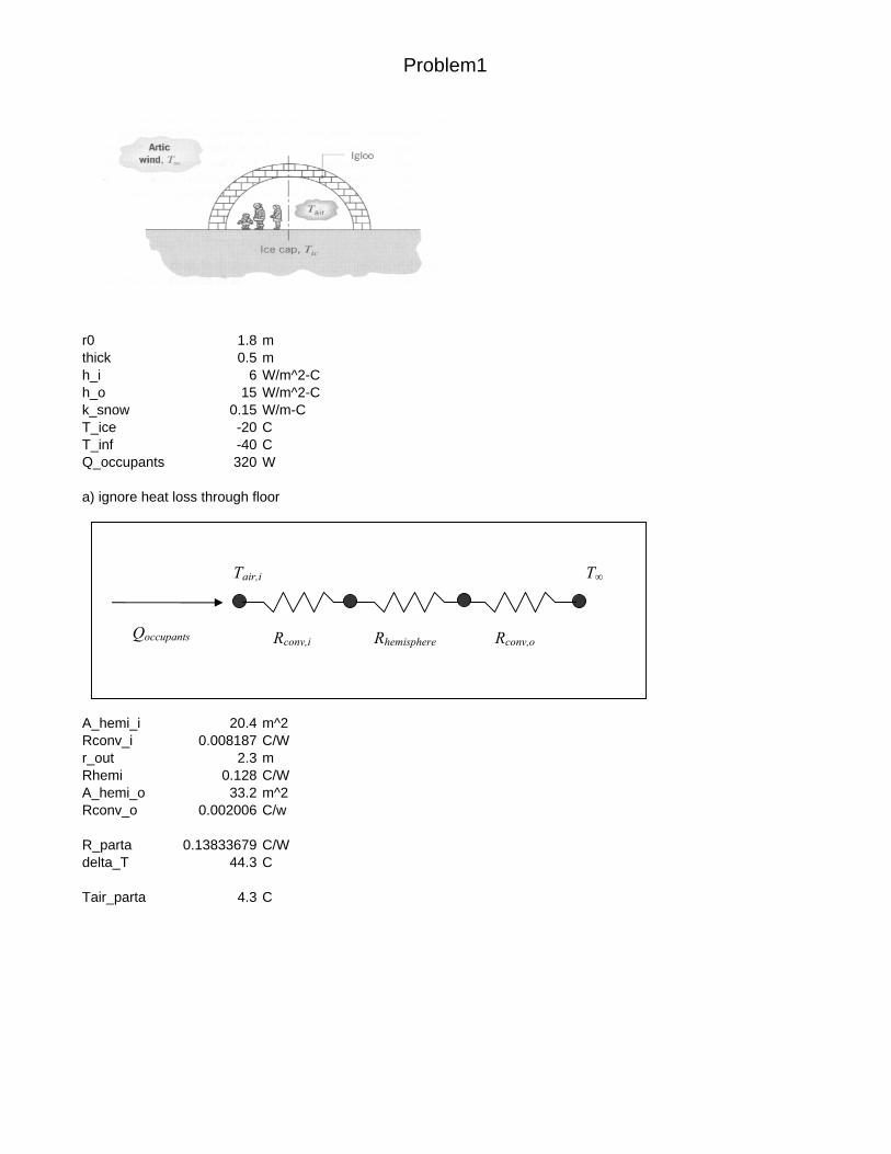
Problem1 r0 1.8 m thick 0.5 m h_i 6 W/m^2-C h_o 15 W/m^2-C k_snow 0.15 W/m-C T_ice -20 C T_inf -40 C Q_occupants 320 W a) ignore heat loss through floor A_hemi_i 20.4 m^2 Rconv_i 0.008187 C/W r_out 2.3 m Rhemi 0.128 C/W A_hemi_o 33.2 m^2 Rconv_o 0.002006 C/w R_parta 0.13833679 C/W delta_T 44.3 C Tair_parta 4.3 C T air,i R hemisphere R conv,i T ∞ R conv,o Q occupants
Biot 0.319Note that the Biot is based on L_slab/2 since cooled on both sides
a) minimum time for one term solutiont_min 17.16 seconds
b) need A_1 and lambda_1 from Table 4-1 Bi A_1 lambda_1by interpolation: 0.3 1.045 0.7465A_1 1.0475 0.319 1.047454 0.76634lambda_1 0.7663 0.4 1.058 0.8516
Heat Transfer: A Practical Approach - Yunus A Cengel Fall 2003, Assignment 5
1
Tuesday, September 30, 2003 Chapter 4, Problem 40. Long cylindrical AISI stainless steel rods (k = 7.74 Btu/h ⋅ ft ⋅ °F and α = 0.135 ft2/h) of 4-in. diameter are heat-treated by drawing them at a velocity of 10 ft/min through a 30-ft-long oven maintained at 1700°F. The heat transfer coefficient in the oven is 20 Btu/h ⋅ ft2 ⋅ °F. If the rods enter the oven at 85°F, determine their centerline temperature when they leave.
Chapter 4, Solution 40 Figure P4.40 Long cylindrical steel rods are heat-treated in an oven. Their centerline temperature when they leave the oven is to be determined. Assumptions 1 Heat conduction in the rods is one-dimensional since the rods are long and they have thermal symmetry about the center line. 2 The thermal properties of the rod are constant. 3 The heat transfer coefficient is constant and uniform over the entire surface. 4 The Fourier number is τ > 0.2 so that the one-term approximate solutions (or the transient temperature charts) are applicable (this assumption will be verified). Properties The properties of AISI stainless steel rods are given to be k = 7.74 Btu/h.ft.°F, α = 0.135 ft2/h. Analysis The time the steel rods stays in the oven can be determined from
t = = =length
velocity ft
ft / min min = 180 s30
103
Steel rod, 85°F
Oven, 1700°F The Biot number is
4307.0)FBtu/h.ft. 74.7(
)ft 12/2)(F.Btu/h.ft 20( 2=
°°
==k
hrBi o
The constants λ1 and A1 corresponding to this Biot number are, from Table 4-1, λ1 1 08784 10995= =. . and A
The Fourier number is
τα
= = =t
ro2
01352 12
0 243( .( /
. ft / h)(3 / 60 h) ft)
2
2
Then the temperature at the center of the rods becomes
Heat Transfer: A Practical Approach - Yunus A Cengel Fall 2003, Assignment 5
2
Tuesday, September 30, 2003 Chapter 4, Problem 54. White potatoes (k = 0.50 W/m ⋅ °C and α = 0.13 × 10⁻⁶ m2/s) that are initially at a uniform temperature of 25°C and have an average diameter of 6 cm are to be cooled by refrigerated air at 2°C flowing at a velocity of 4 m/s. The average heat transfer coefficient between the potatoes and the air is experimentally determined to be 19 W/m2 ⋅ °C. Determine how long it will take for the center temperature of the potatoes to drop to 6°C. Also, determine if any part of the potatoes will experience chilling injury during this process.
Figure P4.54 Chapter 4, Solution 54 The center temperature of potatoes is to be lowered to 6°C during cooling. The cooling time and if any part of the potatoes will suffer chilling injury during this cooling process are to be determined. Assumptions 1 The potatoes are spherical in shape with a radius of r0 = 3 cm. 2 Heat conduction in the potato is one-dimensional in the radial direction because of the symmetry about the midpoint. 3 The thermal properties of the potato are constant. 4 The heat transfer coefficient is constant and uniform over the entire surface. 5 The Fourier number is τ > 0.2 so that the one-term approximate solutions (or the transient temperature charts) are applicable (this assumption will be verified). Properties The thermal conductivity and thermal diffusivity of potatoes are given to be k = 0.50 W/m⋅°C and α = 0.13×10⁻⁶ m2/s. Analysis First we find the Biot number: Air
2°C 4 /
Bi W / m . C) m0.5 W / m C
2= =
°°
=hrk
0 19 0 03 114( ( . ).
.
From Table 4-1 we read, for a sphere, λ1 = 1.635 and A1 = 1.302. Substituting these values into the one-term solution gives
θ τλ τ τ0 1
63512 26 2
25 21302 0 753=
−−
= →−−
= →∞
∞
− −T TT T
A e eo
i =. .(1. )
Potato Ti = 25°C
which is greater than 0.2 and thus the one-term solution is applicable. Then the cooling time becomes
h 1.45==×
==⎯→⎯= s 5213s/m 100.13
m) 03.0)(753.0( 26-
220
20 α
τατr
tr
t
The lowest temperature during cooling will occur on the surface (r/r0 = 1), and is determined to be
Heat Transfer: A Practical Approach - Yunus A Cengel Fall 2003, Assignment 5
3
Tuesday, September 30, 2003 which is above the temperature range of 3 to 4 °C for chilling injury for potatoes. Therefore, no part of the potatoes will experience chilling injury during this cooling process. Alternative solution We could also solve this problem using transient temperature charts as follows:
15a)-4 (Fig. 75.0t
=174.0
22526
877.0m)C)(0.03.W/m(19
CW/m.50.0Bi1
2
o2
o
=
⎪⎪
⎭
⎪⎪
⎬
⎫
=−−
=−−
===
∞
∞ o
i
o
o
rTTTThrk
ατ
Therefore, tr
ss= =
×= ≅−
τα
02 2
60 75 0 03
013 105192
( . )( . ). /m 2 1.44 h
The surface temperature is determined from
1
0 877
10 60
0
0
BiFig. 4 -15b)
= =
=
⎫
⎬⎪⎪
⎭⎪⎪
−−
=∞
∞
khr
rr
T r TT T
.( )
. (
which gives T T T Tsurface o= + − = + − =∞ ∞0 6 2 0 6 6 2 4 4. ( ) . ( ) . º C The slight difference between the two results is due to the reading error of the charts.
Heat Transfer: A Practical Approach - Yunus A Cengel Fall 2003, Assignment 5
4
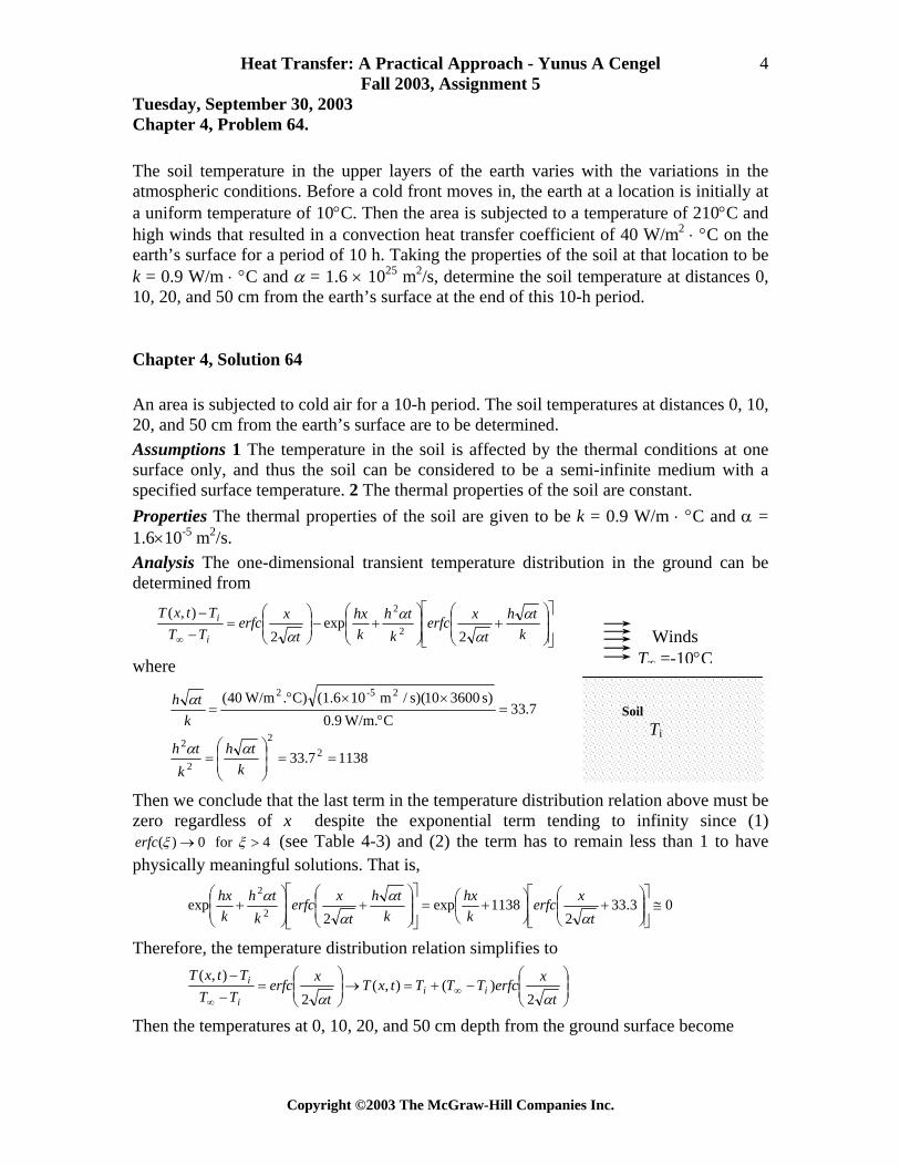
Tuesday, September 30, 2003 Chapter 4, Problem 64. The soil temperature in the upper layers of the earth varies with the variations in the atmospheric conditions. Before a cold front moves in, the earth at a location is initially at a uniform temperature of 10°C. Then the area is subjected to a temperature of 210°C and high winds that resulted in a convection heat transfer coefficient of 40 W/m2 ⋅ °C on the earth’s surface for a period of 10 h. Taking the properties of the soil at that location to be k = 0.9 W/m ⋅ °C and α = 1.6 × 1025 m2/s, determine the soil temperature at distances 0, 10, 20, and 50 cm from the earth’s surface at the end of this 10-h period.
Chapter 4, Solution 64 An area is subjected to cold air for a 10-h period. The soil temperatures at distances 0, 10, 20, and 50 cm from the earth’s surface are to be determined. Assumptions 1 The temperature in the soil is affected by the thermal conditions at one surface only, and thus the soil can be considered to be a semi-infinite medium with a specified surface temperature. 2 The thermal properties of the soil are constant. Properties The thermal properties of the soil are given to be k = 0.9 W/m ⋅ °C and α = 1.6×10⁻⁵ m2/s. Analysis The one-dimensional transient temperature distribution in the ground can be determined from
⎥⎥⎦
⎤
⎢⎢⎣
⎡⎟⎟⎠
⎞⎜⎜⎝
⎛+⎟
⎟⎠
⎞⎜⎜⎝
⎛+−⎟⎟
⎠
⎞⎜⎜⎝
⎛=
−−
∞ kth
txerfc
kth
khx
txerfc
TTTtxT
i
i αα
αα 2
exp2
),(2
2
Winds T∞ =-10°Cwhere
Soil Ti
11387.33
7.33C W/m.0.9
)s 360010)(s/m 10(1.6C). W/m40(
22
2
2
2-52
==⎟⎟⎠
⎞⎜⎜⎝
⎛=
=°
××°=
kth
kth
kth
αα
α
Then we conclude that the last term in the temperature distribution relation above must be zero regardless of x despite the exponential term tending to infinity since (1)
4for 0)( >→ ξξerfc (see Table 4-3) and (2) the term has to remain less than 1 to have physically meaningful solutions. That is,
03.332
1138exp2
exp2
2≅
⎥⎥⎦
⎤
⎢⎢⎣
⎡⎟⎟⎠
⎞⎜⎜⎝
⎛+⎟
⎠⎞
⎜⎝⎛ +=
⎥⎥⎦
⎤
⎢⎢⎣
⎡⎟⎟⎠
⎞⎜⎜⎝
⎛+⎟
⎟⎠
⎞⎜⎜⎝
⎛+
txerfc
khx
kth
txerfc
kth
khx
αα
αα
Therefore, the temperature distribution relation simplifies to
⎟⎟⎠
⎞⎜⎜⎝
⎛−+=→⎟⎟
⎠
⎞⎜⎜⎝
⎛=
−−
∞∞ t
xerfcTTTtxTt
xerfcTT
TtxTii
i
i
αα 2)(),(
2
),(
Then the temperatures at 0, 10, 20, and 50 cm depth from the ground surface become
Heat Transfer: A Practical Approach - Yunus A Cengel Fall 2003, Assignment 5
6
Tuesday, September 30, 2003
s C,
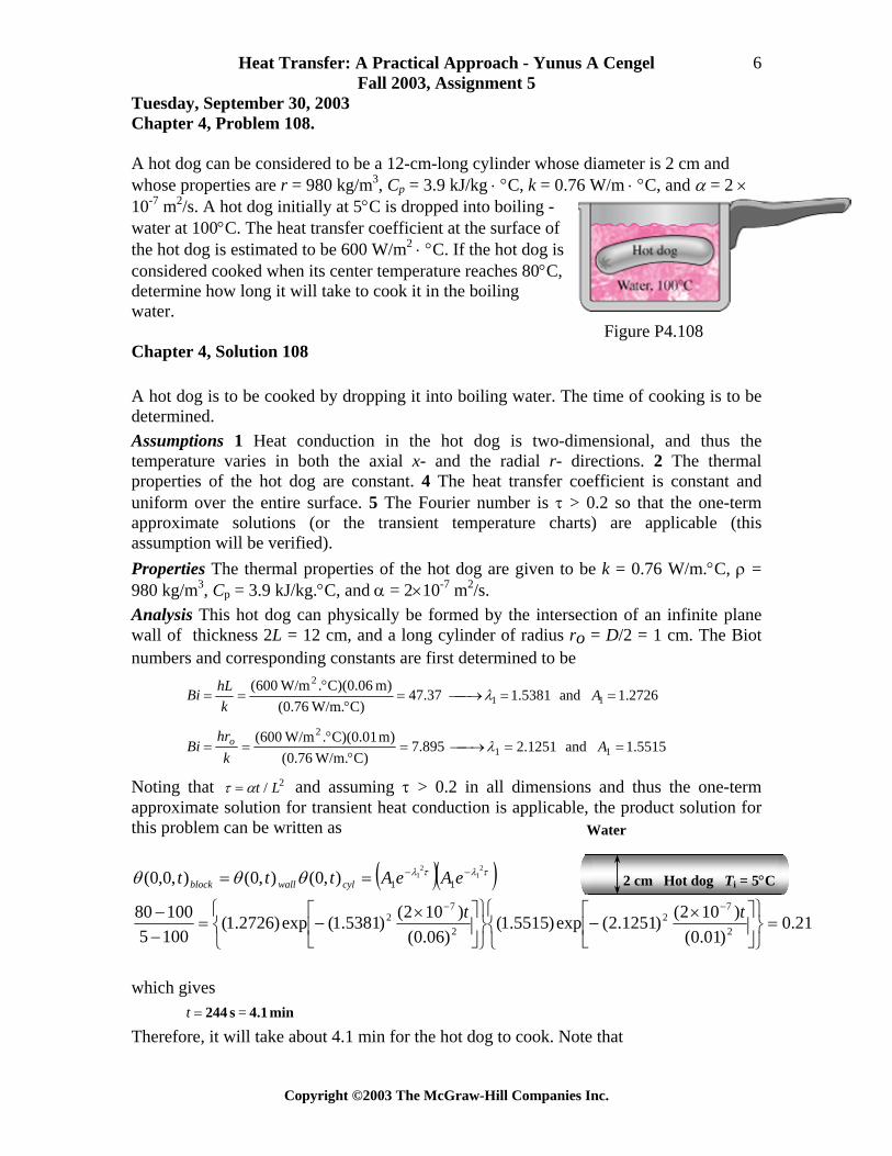
Chapter 4, Problem 108. A hot dog can be considered to be a 12-cm-long cylinder whose diameter is 2 cm and whose properties are r = 980 kg/m3, Cp = 3.9 kJ/kg ⋅ °C, k = 0.76 W/m ⋅ °C, and α = 2 × 10⁻⁷ m2/s. A hot dog initially at 5°C is dropped into boiling -water at 100°C. The heat transfer coefficient at the surface of the hot dog is estimated to be 600 W/m2 ⋅ °C. If the hot dog iconsidered cooked when its center temperature reaches 80°determine how long it will take to cook it in the boilingwater.
Figure P4.108 Chapter 4, Solution 108 A hot dog is to be cooked by dropping it into boiling water. The time of cooking is to be determined. Assumptions 1 Heat conduction in the hot dog is two-dimensional, and thus the temperature varies in both the axial x- and the radial r- directions. 2 The thermal properties of the hot dog are constant. 4 The heat transfer coefficient is constant and uniform over the entire surface. 5 The Fourier number is τ > 0.2 so that the one-term approximate solutions (or the transient temperature charts) are applicable (this assumption will be verified). Properties The thermal properties of the hot dog are given to be k = 0.76 W/m.°C, ρ = 980 kg/m3, Cp = 3.9 kJ/kg.°C, and α = 2×10⁻⁷ m2/s. Analysis This hot dog can physically be formed by the intersection of an infinite plane wall of thickness 2L = 12 cm, and a long cylinder of radius ro = D/2 = 1 cm. The Biot numbers and corresponding constants are first determined to be
37.47)C W/m.76.0(
)m 06.0)(C. W/m600( 2=
°°
==k
hLBi 2726.1 and 5381.1 11 ==⎯→⎯ Aλ
895.7)C W/m.76.0(
)m 01.0)(C. W/m600( 2=
°°
==k
hrBi o 5515.1 and 1251.2 11 ==⎯→⎯ Aλ
Noting that and assuming τ > 0.2 in all dimensions and thus the one-term approximate solution for transient heat conduction is applicable, the product solution for this problem can be written as
Heat Transfer: A Practical Approach - Yunus A Cengel Fall 2003, Assignment 5
7
Tuesday, September 30, 2003
2.049.0m) 01.0(
s) /s)(244m 102(2
27
2>=
×==
−
ocyl
rtατ
and thus the assumption τ > 0.2 for the applicability of the one-term approximate solution is verified. Note that the dimensionless time corresponding to the plane wall solution is
2.00136.0m) 06.0(
s) /s)(244m 102(2
27
2 <=×
==−
Lt
wallατ
and so the one-term solution for the plane wall is not valid. If we instead solve treating the hot dog as a very long cylinder, we get:
( )21.0
)01.0()102()1251.2(exp)5515.1(
100510080
),0(
2
72
1
21
=⎭⎬⎫
⎩⎨⎧
⎥⎦
⎤⎢⎣
⎡ ×−=
−−
=−
−
t
eAt cylτλθ
which gives min 3.68 s 221 = =t Discussion This problem could also be solved by treating the hot dog as an infinite cylinder since heat transfer through the end surfaces will have little effect on the mid section temperature because of the large distance.