Problems of Enumeration and Realizability on ... - Mathematics

Problems of Enumeration and Realizability

on Matroids, Simplicial Complexes, and Graphs

By

YVONNE SUZANNE KEMPER

B.A. (University of California, Berkeley) 2008

DISSERTATION

Submitted in partial satisfaction of the requirements for the degree of

DOCTOR OF PHILOSOPHY

in

Mathematics

in the

OFFICE OF GRADUATE STUDIES

of the

UNIVERSITY OF CALIFORNIA

DAVIS

Approved:

Jesus De Loera, Chair

Eric Babson

Monica Vazirani

Matthias Beck

Committee in Charge

2013

-i-

Contents

Abstract iii

Acknowledgments iv

Chapter 1. Introduction 1

1.1. Matroids 2

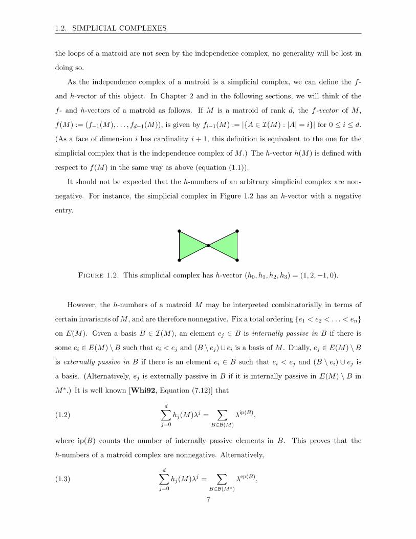
1.2. Simplicial complexes 5

1.3. Graphs 9

Chapter 2. h-Vectors of Small Matroid Complexes 18

2.1. Rank-2 matroids 18

2.2. Corank-2 matroids 19

2.3. Rank-3 matroids 20

2.4. Matroids on at most nine elements 23

2.5. Further questions and directions 25

Chapter 3. Polytopal Embeddings of Cayley Graphs 27

3.1. Not all Cayley graphs are polyhedral 27

3.2. Two families of polyhedral Cayley graphs 32


Chapter 4. Flows on Simplicial Complexes 44

4.1. Structure of the boundary matrices of simplicial complexes 44

4.2. The number of nowhere-zero Zq-flows on a simplicial complex 48

4.3. The period of the flow quasipolynomial 53

4.4. Flows on triangulations of manifolds 57


Bibliography 60

-ii-

Yvonne Suzanne KemperJune 2013

Mathematics

Problems of Enumeration and Realizability on Matroids, Simplicial Complexes, and Graphs

Abstract

This thesis explores several problems on the realizability and structural enumeration of

geometric and combinatorial objects. After providing an overview of the thesis and some of the

relevant background material in Chapter 1, we consider in Chapter 2 a conjecture of Stanley on

the h-vectors of matroid complexes. We use the geometric structure of these objects to verify

the conjecture in the case that the matroid corank is at most two, and provide new, simple

proofs for the case when the matroid rank is at most three. We discuss an implementation based

on simulated annealing and Barvinok-type methods to verify the conjecture for all matroids on

at most nine elements using computers.

In Chapter 3, we study the geometry of Cayley graphs, in particular the embeddability

of Cayley graphs as the 1-dimensional skeletons of convex polytopes. We find an example

of a Cayley graph for which no such embedding exists, and provide an extension of Maschke’s

classification of planar groups with a new proof that emphasizes the connectivity and associated

actions of the Cayley graphs and uses polyhedral techniques such as Steinitz’s theorem. We

further study the groups of symmetry of regular, convex polytopes and recall the Wythoff

construction, which gives a polytope with 1-skeleton equal to the Cayley graph of the associated

symmetry group.

Finally, in Chapter 4 we define a higher-dimensional extension of the graph-theoretic notion

of nowhere-zero Zq-flows, and begin a systematic study of the enumerative and structural

qualities of flows on simplicial complexes. We extend Tutte’s result for the enumeration of

Zq-flows on graphs to simplicial complexes, and find examples of complexes that, unlike graphs,

do not admit a polynomial flow enumeration function. In light of work by Dey, Hirani, and

Krishnamoorthy, we study the boundary matrices of a subfamily of simplicial complexes, and

consider possible bounds for the period of their flow quasipolynomials.

At the end of each chapter, we present open questions and future directions related to each

of the research topics.

-iii-

Acknowledgments

I would first like to thank all of my mathematical mentors, especially Jesus De Loera and

Matthias Beck. Without their energy, support, guidance, hard work, and seemingly endless

amounts of time and patience, I would not have completed my degree. Thank you also to the

many others at Davis for your advice, encouragement, and assistance: Eric Babson, Amitabh

Basu, Andrew Berget, Steven Klee, Matthias Koppe, Alexander Soshnikov, and Monica Vazi-

rani. Thank you also to collaborators outside of Davis: Felix Breuer, Logan Godkin, and Jeremy

Martin.

Moreover, I would like to recognize the unbeatable staff at the math department: Perry Gee,

Tina Denena, Carol Crabill, Jessica Goodall, thank you. In addition, throughout my graduate

career, I was fortunate to have fun, fruitful, and sometimes even mathematical interactions with

mathematicians outside Davis: thank you Adam Bohn, Benjamin Braun, Christian Haase, and

Henri Muhle. Thank you also to my academic siblings: Brandon Dutra, David Haws, Mark

Junod, Eddie Kim, Jake Miller, and Ruriko Yoshida.

I would like to thank my family. Thank you for believing in me, supporting my decisions

(despite their extremely mercurial nature), and all your advice and help in getting through the

many challenges — big and small — of my graduate career.

I would like to thank the many fine friends I have made in Davis, in particular David

Renfrew. I would like to thank the Owl House. Friends and roommates: Corey, Maggie, Cat,

Owen, Patrick, Amanda, Nate, Paul, Rainbow, Katherine, and Francisco, thank you for the

love and the support, for goats and dinner parties, for Settlers and Owling.

Ich danke Konrad — ohne Deutsch, ware ich morgens nie aus Bett gegangen. Ich wurde

gern den Steinfreunden danken: Aga, Neil, und Dustin. Ihr wisst warum.

Finally, I want to acknowledge the support of the NSF, and in particular through NSF grant

DMS-0914107 and NSF VIGRE grant DMS-0636297, as well as the many grants of support I

have received from UC Davis, the UC Davis Mathematics Department, and conferences around

the world.

-iv-

CHAPTER 1

Introduction

What does a combinatorial space look like? How is it put together? How many are there?

These fundamental questions, and others like them, give rise to two important themes in geo-

metric combinatorics: realizability and enumeration. Research in these areas has led to a

plethora of theorems that connect the geometric and combinatorial properties of objects such

as matroids, simplicial complexes, and graphs. Famous results include the following theorems.

These theorems, and their extensions in the papers of Maschke [Mas96], Stanley [Sta77],

Tutte [Tut47], and too many others to list, provided particular inspiration for work and results

presented in this thesis.

Theorem 1.0.1 ([Kur30]). A finite graph is planar if and only if it does not contain a

subgraph that is a subdivision of K5, the complete graph on five vertices, or K3,3, the complete

bipartite graph with parts of size three.

Theorem 1.0.2 ([Ehr62]). Let P be the convex hull of finitely many points in Rd with

vertices in Zd. Then, the lattice-point counting function

EhrP(t) := #(tP ∩ Zd

)is a polynomial in positive integer variable t.

The goal of this thesis is to gain a deeper understanding of the structure and combina-

torics of matroids, simplicial complexes, and graphs by exploring them from the perspectives

of realizability and enumerative combinatorics. Jointly with Matthias Beck, Jesus De Loera,

and Steven Klee [BK12, DLKK12], we study (1) structural quantities of simplicial complexes

derived from matroids; (2) embeddings of Cayley graphs as 1-skeletons of d-polytopes; and (3)

combinatorial quantities of simplicial complexes. In the next sections, we present the back-

ground and motivation for our work, and state our main results. In the chapters following this

introduction, we provide further details and proofs.

1

1.1. MATROIDS

1.1. Matroids

We begin with an object prominent in combinatorics: the matroid [Oxl92, Wel76, Whi92].

There are many ways to define a matroid; we give the (perhaps) most intuitive here. In this

thesis, all matroids are finite: for every M , E(M) is a finite set.

Definition 1.1.1. A matroid M = (E(M), I(M)) consists of a ground set E(M) and a

family of subsets I(M) ⊆ 2E(M) called independent sets such that

(1) ∅ ∈ I;

(2) if I ∈ I and J ⊂ I, then J ∈ I; and

(3) if I, J ∈ I, and |J | < |I|, then there exists some e ∈ I \ J such that J ∪ {e} ∈ I.

A basis of M is a maximal independent set under inclusion – by (3) above, all bases will have

the same cardinality. The rank of a subset S ⊆ E(M) is the size of a largest independent set A ⊆

S; in particular, the rank of M is the cardinality of a basis. A loop is a singleton {e} 6∈ I(M),

and a coloop is an element that is contained in every basis. If M is a loopless matroid, elements

e, e′ ∈ E(M) are pairwise parallel if {e, e′} /∈ I(M). The parallelism classes of M are maximal

subsets E1, . . . , Et ⊆ E(M) with the property that all elements in each set Ei are parallel. It

can be easily checked that if {ei1 , . . . , eik} ∈ I(M) with eij ∈ Ej , then {e′i1 , . . . , e′ik} ∈ I(M)

for any choice of e′ij ∈ Ej . To see this, it is enough to show that if {ei1 , . . . , eij , . . . , eik}

is an independent set with eil ∈ Eil for all 1 ≤ l ≤ k, then {ei1 , . . . , e′ij , . . . , eik} is also

independent, where e′ij is any element in Eij . We know {e′ij , ei1} is independent, as they are in

separate parallelism classes. Therefore, there exists eim 6= eij ∈ {ei1 , . . . , eij , . . . , eik} such that

{e′ij , ei1 , eim} is independent (by (3) above). We can iteratively build the set in this way, and

preserve the independence, until we have {ei1 , . . . , e′ij , . . . , eik}. Alternatively, the parallelism

classes of M are maximal rank-one subsets of E(M).

Given a matroid M on the ground set E(M) with bases B(M), we define its dual matroid,

M∗, to be the matroid on E(M) whose bases are B(M∗) = {E \ B : B ∈ B(M)}. In this

context, {e} is a coloop in M if {e} is a loop in M∗.

There are many objects that can be thought of very naturally in terms of matroids. For

instance, any matrix or any graph gives a matroid: for the former, elements of E(M) are the

columns of the matrix, and I(M) consists of the independent subsets of columns. For the latter,

elements of E(M) are the edges of the graph, and I(M) consists of the subforests of the graph.

2

1.1. MATROIDS

Matroids were in fact originally conceived as a generalization of the linear independences given

by the columns of a matrix or the edges of a graph.

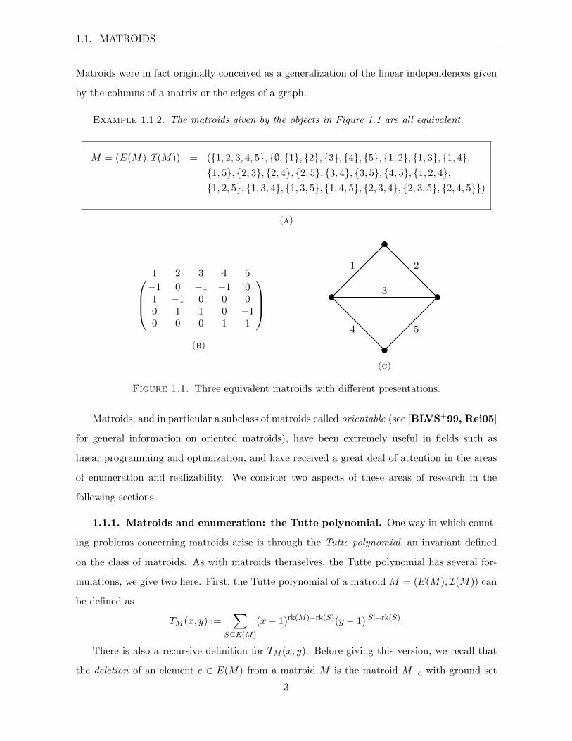
Example 1.1.2. The matroids given by the objects in Figure 1.1 are all equivalent.

M = (E(M), I(M)) = ({1, 2, 3, 4, 5}, {∅, {1}, {2}, {3}, {4}, {5}, {1, 2}, {1, 3}, {1, 4},{1, 5}, {2, 3}, {2, 4}, {2, 5}, {3, 4}, {3, 5}, {4, 5}, {1, 2, 4},{1, 2, 5}, {1, 3, 4}, {1, 3, 5}, {1, 4, 5}, {2, 3, 4}, {2, 3, 5}, {2, 4, 5}})

(a)

1 2 3 4 5

−1 0 −1 −1 01 −1 0 0 00 1 1 0 −10 0 0 1 1

(b)

1 2

3

4 5

(c)

Figure 1.1. Three equivalent matroids with different presentations.

Matroids, and in particular a subclass of matroids called orientable (see [BLVS+99, Rei05]

for general information on oriented matroids), have been extremely useful in fields such as

linear programming and optimization, and have received a great deal of attention in the areas

of enumeration and realizability. We consider two aspects of these areas of research in the

following sections.

1.1.1. Matroids and enumeration: the Tutte polynomial. One way in which count-

ing problems concerning matroids arise is through the Tutte polynomial, an invariant defined

on the class of matroids. As with matroids themselves, the Tutte polynomial has several for-

mulations, we give two here. First, the Tutte polynomial of a matroid M = (E(M), I(M)) can

be defined as

TM (x, y) :=∑

S⊆E(M)

(x− 1)rk(M)−rk(S)(y − 1)|S|−rk(S).

There is also a recursive definition for TM (x, y). Before giving this version, we recall that

the deletion of an element e ∈ E(M) from a matroid M is the matroid M−e with ground set

3

1.1. MATROIDS

E(M−e) = E(M) \ {e}, and independent sets I(M−e) = {I ∈ I(M) : e 6∈ I}. Then, the

contraction of a matroid M about an element e is the matroid M/e with ground set E(M/e) =

E(M)\{e} and independent sets I(M/e) = {I ∈ I(M) : e 6∈ I and I ∪{e} ∈ I(M)}. Note that

the class of matroids is closed under the operations of deletion and contraction. Given these,

we have the following alternative definition of the Tutte polynomial:

TM (x, y) =

x if M = ({e}, {∅, {e}}), i.e. M is a coloop,

y if M = ({e}, {∅}), i.e. M is a loop,

TM−e(x, y) + TM/e(x, y) if e is neither a loop nor a coloop,

xTM−e(x, y) if e is a coloop, and

yTM−e(x, y) if e is a loop.

Some evaluations of the Tutte polynomial have known interpretations. For instance,

TM (1, 1) counts the number of bases of M (see [Whi92, Chapter 6] for an extensive list of

interpretations). Often, as is the case with our example, these evaluations correspond to enu-

merations of structural characteristics of the matroid, and specializations of the Tutte polyno-

mial to univariate polynomials give enumeration functions in some cases. We discuss several

particular specializations in Section 1.3.2.

1.1.2. Matroids and realizations: matrices, arrangements, and polytopes. Often,

we want to realize matroids as matrices over a field. For instance, the matroid in Example 1.1.2

is regular — it can be realized over any field. We can also think of realizations in terms of

hyperplane arrangements (i.e., a collection of subspaces of codimension one in Rn) or convex

polytopes (that is, convex hulls of finitely many points) with defining coordinates in a particular

field. There has been extensive research on this question, particularly on orientable matroids,

see [Bok08, RG96, BS86, BS87, BS89, FMM13, KP11, Mne85, Sey79] for just a few

of the many results. When a matroid is realizable, the Tutte polynomial becomes particularly

meaningful for some evaluations, see [Jae89, Rei99, Whi92].

In some sense, any matroid can be realized geometrically; matroids make up a subfamily of

the objects we discuss next: simplicial complexes.

4

1.2. SIMPLICIAL COMPLEXES

1.2. Simplicial complexes

Simplicial complexes exemplify the bridge between geometry and combinatorics. We recall

their definition:

Definition 1.2.1. An (abstract) simplicial complex ∆ on a vertex set V is a set of subsets

of V . These subsets are called the faces of ∆, and we require that

(1) for all v ∈ V , {v} ∈ ∆, and

(2) for all F ∈ ∆, if G ⊆ F , then G ∈ ∆.

The dimension of a face F is dim(F ) = |F | − 1, and the dimension of ∆ is dim(∆) =

max{dim(F ) : F ∈ ∆}. A simplicial complex is pure if all maximal faces (that is, faces that

are not properly contained in any other face) have the same cardinality. In this case, a maximal

face is called a facet, and a ridge is a face of codimension one. In this thesis, we will work only

with pure and finite (i.e., |∆| <∞)simplicial complexes.

In addition to the combinatorial definition, we have geometric realizations of every simpli-

cial complex as collections of simplices (i.e., vertices, line segments, triangles, and their higher

dimensional analogues). For more background on simplicial complexes, see [Sta96, Chapter

0.3] or [Hat02, Chapter 2]. Simplicial complexes arise in many areas: they are useful as com-

putational examples and test cases, they can encode combinatorial problems and information,

and they have connections to fields such as optimization and linear programming. The fact that

simplicial complexes appear in so many contexts has been extremely fruitful for both combina-

torics and geometry, allowing us to compare complexes that arise from different combinatorial

problems, understand combinatorial families of complexes by developing intuition about their

geometry, and more [Gra02, HKW03, KS10, San12, LLS08]. It is therefore of interest to

gain a deep understanding of the structural aspects of simplicial complexes.

One structural quantity of a simplicial complexes that is very natural to measure is the

number of faces of each dimension. This inspires the following definition:

Definition 1.2.2. The f -vector of a (d− 1)-dimensional simplicial complex ∆ is a vector

f(∆) := (f−1(∆), . . . , fd−1(∆)), where fi = |{F ∈ ∆ : dim(F ) = i}| and f−1 = 1. The fi(∆)s

are called the f -numbers of ∆.

5


Oftentimes, it is more convenient to study the h-vector h(∆) := (h0(∆), . . . , hd(∆)) of a

simplicial complex ∆, whose entries are defined by the relation

(1.1)

d∑j=0

hj(∆)λj =

d∑i=0

fi−1(∆)λi(1− λ)d−i.

See [Sta96] for more on h-vectors and the combinatorics of simplicial complexes. Given that

f - and h-vectors are defined for all simplicial complexes, it is natural to ask whether we can

describe exactly the possible f - and h-vectors of these objects. Schutzenberger [Sch59], and

later Kruskal [Kru63] and Katona [Kat68], provided the characterization of the f -vectors (and

hence, the h-vectors) of simplicial complexes. We give one necessary definition, then state their

theorem.

Definition 1.2.3. Given two integers k, i > 0, write

k =

(nii

)+

(ni−1

i− 1

)+ · · ·+

(njj

),

where ni > ni−1 > · · · > nj ≥ j ≥ 1. Define

k(i) =

(nii+ 1

)+

(ni−1

i

)+ · · ·+

(njj + 1

).

Theorem 1.2.4 ([Kat68, Kru63, Sch59]). A vector (1, f0, f1, . . . , fd−1) ∈ Zd+1 is the

f -vector of some (d− 1)-dimensional simplicial complex ∆ if and only if

0 < fi+1 ≤ f (i+1)i , 0 ≤ i ≤ d− 2.

Certain subclasses of simplicial complexes have more specific f - and h-vector characteriza-

tions, such as Cohen–Macaulay complexes (see [Mac26, Sta96] for more on Cohen–Macaulay

complexes). However, many subclasses remain uncharacterized, such as flag complexes [Sta96]

and, the focus of the next section, independence complexes of matroids.

1.2.1. Independence complexes of matroids. Matroids make up a highly-structured

subfamily of simplicial complexes. In particular, the independent sets of a matroid M form the

face set of a simplicial complex ∆ called the independence complex of M (see [Whi92, Chapter

7]). In Chapter 2 we explore in greater detail certain structural quantities of the independence

complexes of small matroids. In that chapter, we will consider only loopless matroids: since

6


the loops of a matroid are not seen by the independence complex, no generality will be lost in

doing so.

As the independence complex of a matroid is a simplicial complex, we can define the f -

and h-vector of this object. In Chapter 2 and in the following sections, we will think of the

f - and h-vectors of a matroid as follows. If M is a matroid of rank d, the f -vector of M ,

f(M) := (f−1(M), . . . , fd−1(M)), is given by fi−1(M) := |{A ∈ I(M) : |A| = i}| for 0 ≤ i ≤ d.

(As a face of dimension i has cardinality i + 1, this definition is equivalent to the one for the

simplicial complex that is the independence complex of M .) The h-vector h(M) is defined with

respect to f(M) in the same way as above (equation (1.1)).

It should not be expected that the h-numbers of an arbitrary simplicial complex are non-

negative. For instance, the simplicial complex in Figure 1.2 has an h-vector with a negative

entry.

Figure 1.2. This simplicial complex has h-vector (h0, h1, h2, h3) = (1, 2,−1, 0).

However, the h-numbers of a matroid M may be interpreted combinatorially in terms of

certain invariants ofM , and are therefore nonnegative. Fix a total ordering {e1 < e2 < . . . < en}

on E(M). Given a basis B ∈ I(M), an element ej ∈ B is internally passive in B if there is

some ei ∈ E(M) \B such that ei < ej and (B \ ej)∪ ei is a basis of M . Dually, ej ∈ E(M) \B

is externally passive in B if there is an element ei ∈ B such that ei < ej and (B \ ei) ∪ ej is

a basis. (Alternatively, ej is externally passive in B if it is internally passive in E(M) \ B in

M∗.) It is well known [Whi92, Equation (7.12)] that

(1.2)

d∑j=0

hj(M)λj =∑

B∈B(M)

λip(B),

where ip(B) counts the number of internally passive elements in B. This proves that the

h-numbers of a matroid complex are nonnegative. Alternatively,

(1.3)

d∑j=0

hj(M)λj =∑

B∈B(M∗)

λep(B),

7


where ep(B) counts the number of externally passive elements in B. Since the f -numbers (and

hence the h-numbers) of a matroid depend only on its independent sets, equations (1.2) and

(1.3) hold for any ordering of the ground set of M . It is worth remarking that the h-polynomial

above is actually a specialization of the Tutte polynomial of the corresponding matroid (see

[Whi92]). For further information on independence complexes and h-vectors, we refer the

reader to the books of Oxley [Oxl92], White [Whi92], and Stanley [Sta96].

1.2.2. O-Sequences and Stanley’s conjecture. In order to state our results and the

problem to which they pertain, we need several more definitions.

Definition 1.2.5. An order ideal O is a family of monomials (say of degree at most r) in

a finite number of variables with the property that if µ ∈ O and ν|µ, then ν ∈ O.

Let Oi denote the collection of monomials in O of degree i. Let Fi(O) := |Oi| and F (O) =

(F0(O), F1(O), . . . , Fr(O)). We say that O is pure if all of its maximal monomials (under

divisibility) have the same degree. A vector h = (h0, . . . , hd) is a pure O-sequence if there is a

pure order ideal O such that h = F (O).

A longstanding conjecture of Stanley [Sta77] suggests that matroid h-vectors are highly

structured.

Conjecture 1.2.6. For any matroid M , h(M) is a pure O-sequence.

Conjecture 1.2.6 is known to hold for several families of matroid complexes, such as paving

matroids [MNRIVF12], cographic matroids [Mer01], cotransversal matroids [Oh10], lattice

path matroids [Sch10], and matroids of rank at most three [TSZ10, Sto09]. The purpose of

Chapter 2 is to present proofs of the following theorems, originally published in [DLKK12].

Theorem 2.1.1. Let M be a matroid of rank 2. Then h(M) is a pure O-sequence.

Theorem 2.2.1. Let M be a matroid of rank 2. Then h(M∗) is a pure O-sequence.

Theorem 2.3.1. Let M be a loopless matroid of rank d ≥ 3. Then the vector

(1, h1(M), h2(M), h3(M)) is a pure O-sequence.

Theorem 2.4.1. Let M be a matroid on at most nine elements. Then h(M) is a pure

O-sequence.

8

1.3. GRAPHS

While Stanley’s conjecture was already known to hold for matroids of rank two [Sto09]

and rank three [TSZ10], we use the geometry of the independence complexes of matroids of

small rank to provide much simpler shorter proofs in these cases. Our results show that any

counterexample to Stanley’s conjecture must have at least ten elements, rank at least four, and

corank at least three.

Chapter 2 will use several ideas from the theory of multicomplexes and monomial ideals.

Although a general classification of matroid h-vectors or pure O-sequences seems to be an

incredibly difficult problem, some properties are known and will be used in the proofs in that

chapter. In particular:

Theorem 1.2.7. [BC92, Cha97, Hib89] Let h = (h0, h1, . . . , hd) be a matroid h-vector

or a pure O-sequence with hd 6= 0. Then

(1) h0 ≤ h1 ≤ · · · ≤ hb d2c,

(2) hi ≤ hd−i for all 0 ≤ i ≤ bd2c, and

(3) for all 0 ≤ s ≤ d and α ≥ 1, we have

(1.4)s∑i=0

(−α)s−ihi ≥ 0.

Inequality (1.4) is known as the Brown–Colbourn inequality [BC92, Theorem 3.1].

1.3. Graphs

Graphs, like simplicial complexes, are particularly ubiquitous objects, and have been useful

because of their ability to encode and represent data from a variety of contexts and problems

(for instance [ALS12, BMS11, Dij59, ES12, ER59, FF62, Fra11], though this is just a

small part of the body of work on graphs). Most commonly, a graph G = (V,E) is a set of

vertices V together with a set of edges E between vertices. In this thesis, graphs may have loops

(an edge with endpoints that are the same vertex) and parallel edges (multiple edges between

the same pair of vertices). If a graph is simple — no loops or parallel edges — then it can

also be defined as a 1-dimensional simplicial complex. The dual nature of graphs as geometric

and combinatorial objects has been very fruitful, and plays a large role in theorems and proofs

about them.

On the geometric side, some of the many questions asked about graphs concern their em-

beddability in surfaces of varying genus or as the 1-dimensional skeletons of higher-dimensional

9

1.3. GRAPHS

objects. For instance, recall Kuratowski’s theorem (Theorem 1.0.1), which characterizes all

graphs that can be embedded in the surface of the 2-sphere. In Chapter 3 we look at the

particular case of Cayley graphs, a subfamily of graphs that we introduce in the next section.

1.3.1. Polytopal embeddings of Cayley graphs. Given a group Γ and a set of gener-

ators and relations Λ of Γ, it is well-known [Cay78, Mas96] that we can construct a directed,

edge-colored graph C(Γ,Λ) in the following way. The elements of Γ are the vertices of the

graph, and there is a directed edge of color h from g1 to g2 if there exists a generator h ∈ Λ

such that g1h = g2. This graph is the Cayley color graph of (Γ,Λ), denoted C(Γ,Λ). If we

forget the colors and directions of the edges of a Cayley color graph C(Γ,Λ), we obtain the

Cayley graph of (Γ,Λ), denoted G(Γ,Λ). In this thesis, we will work only with Cayley (color)

graphs of finite groups, though there exists a theory of infinite Cayley graphs as well.

Example 1.3.1. Say we have a presentation of the group Z3 × Z2:

(Γ,Λ) = 〈x, y | xy = yx, x3 = y2 = 1〉.

Then, the Cayley color graph is given by Figure 1.3a, where dashed lines indicate multiplication

on the right by x, and solid lines indicate multiplication on the right by y. Typically, when we

have elements of order two, we collapse the edges corresponding to these elements, as in Figure

1.3b. Finally, forgetting about the colors and directions of the edges gives us the Cayley graph,

as in Figure 1.3c.

It is immediate to recover the group from a Cayley color graph: all the basic information

of the group is contained in the graph. In particular, the relations of the group are the cycles

of the graph, and a word in the group is a walk on the graph. In the rest of this section and

in Chapter 3 we restrict ourselves to Cayley graphs that come from minimal presentations of

the group, namely presentations in which no generator in Λ can be expressed in terms of the

remaining generators.

The geometric properties of groups have been studied for a long time in various contexts.

First, graph theorists have looked at the embeddability of Cayley graphs on surfaces. For every

graph G, we can find an orientable surface S of minimal genus such that G has an embedding

in S. The genus of G is then the genus of S. The genus of a group Γ, γ(Γ), is the minimal

genus among the genera of all possible Cayley graphs of Γ. The classification of the groups of

10

1.3. GRAPHS

1 x x2

y yx yx2

(a) The Cayley color graph C(Γ,Λ), asgiven in Example 1.3.1.

1 x x2

y yx yx2

(b) The simplified Cayley color graphC(Γ,Λ), as given in Example 1.3.1.

1 x x2

y yx yx2

(c) The Cayley graph G(Γ,Λ), as givenin Example 1.3.1.

Figure 1.3

a given genus has been completed for genus zero [Mas96], one [Pro78], and two [Tuc84], but

it remains an open problem for genus greater than two [Whi84]. Further, the embeddings of

(mainly infinite) Cayley graphs have been the subject of research investigations by geometric

group theorists (see [AC04]). The combinatorial representation theory of finite groups has been

a third point of intersection for convex geometry and group theory. In this case, polytopes arise

as the convex hulls of images of finite groups under fixed real representations. Of particular

interest are permutation polytopes — these are polytopes arising from a subgroup H of the

symmetric group Sn, where the representation of H is obtained by restricting a permutation

representation of Sn (see e.g., [BHNP09, GP06] and references therein). In what follows,

we will use the terms “1-skeleton of a polytope” and “graph of a polytope” interchangeably.

The focus of Chapter 3 is the question: when is a Cayley graph the graph of a d-dimensional

convex polytope? We show that this is not always the case, but give a few instances in which

the Cayley graph allows for these “convex polyhedral” embeddings:

11

1.3. GRAPHS

Theorem 3.1.1. The Cayley graph of a minimal presentation of the quaternion group

cannot be embedded as the graph of a convex polytope of any dimension.

Theorem 3.2.12. Let Γ be a finite group with a minimal set of generators and relations

Λ. The associated Cayley graph is the graph of a 3-dimensional polytope if and only if Γ is a

finite group of isometries in 3-dimensional space.

1.3.2. Graph polynomials and their extensions. As mentioned above, any graph G

can be interpreted as a matroid, and the Tutte polynomial of a graphic matroid is particularly

interesting. Several specializations have been studied extensively, including the chromatic poly-

nomial χG(q), the reliability polynomial RG(p), and the flow polynomial φG(q). In terms of the

Tutte polynomial of M(G), the matroid given by G, we have:

χG(q) = (−1)|V |−k(G)qk(G)TM(G)(1− q, 0),

RG(p) = (1− p)|V |−k(G)p|E|−|V |+k(G)TM(G)

(1,

1

p

), and

φG(q) = (−1)|E|+|V |+k(G)TM(G)(0, 1− q),

where E is the edge-set of G, V is the vertex-set of G, and k(G) is the number of connected

components of G. These specializations have particular meaning in the case of graphs: for

positive integers q, χG(q) counts the number of proper q-colorings of G (see [Whi92, Chapter

6]), and for negative q we have additional interpretations (see [Sta73, BZ06a]). For 0 ≤ p ≤ 1,

the polynomial RG(p) gives the probability that a network G will “fail” — that is, become

disconnected – given that each edge is removed with probability p. Interest in understanding

the reliability polynomial inspired the study of h-vectors of matroid independence complexes,

which we advance in Chapter 2, because

RG(p) = p|V |−1

|E|−|V |+1∑i=0

hi(1− p)i ,

where (h0, . . . , h|E|−|V |+1) is the h-vector of M(G).

Lastly, for positive integers q, φG(q) counts the number of nowhere-zero Zq-flows on the

graph (see [Whi92, Chapter 6]). To define a flow on a graph G, we first give an initial

orientation to its edges (this orientation is arbitrary, but fixed). Then, a Zq-flow on G is an

assignment of values from Zq to each edge such that modulo q, the sum of values entering

12

1.3. GRAPHS

each node is equal to the sum of values leaving it. If none of the edges receive zero weight,

the Zq-flow is nowhere-zero. In terms of the signed incidence matrix M of G, a Zq-flow is an

element of the kernel of M mod q. See Figure 1.4 for an example of a nowhere-zero Z5-flow.

1

2

2 3

3

1 2

3

4

(a) An oriented graph with a nowhere-zero Z5-flow.

12 13 14 23 241 −1 −1 −1 0 02 1 0 0 −1 −13 0 1 0 1 04 0 0 1 0 1

(b) The signed incidence matrix corre-sponding to the graph on the left.

Figure 1.4. (1, 2, 2, 3, 3)T is a nowhere-zero Z5-flow and an element of thekernel (mod 5) of the incidence matrix.

Flows on graphs were first studied by Tutte ([Tut47, Tut48]; see also [BSST75] and

[Tut76]) in the context of Kirchoff’s electrical circuit laws, and Tutte [Tut47] first proved the

following:

Theorem 1.3.2. The number of nowhere-zero Zq-flows on a graph, φG(q) is a polynomial

in q.

Since that time, a great deal of work (see, for instance, [BZ06b, Jae88, Sey95, Whi92])

has been done, and applications found in network and information theory, optimization, and

other fields.

In order to extend the definition of a flow to a larger class of objects, we make use of

the definition of a graph as a one-dimensional simplicial complex. Let ∆ be a pure simplicial

complex of dimension d with vertex set V = {v0, . . . , vn}. Assign an ordering to V so that

v0 < v1 < · · · < vn. Then, any r-dimensional face of ∆ can be written (with respect to this

ordering) as [vi0 · · · vir ]. We then have the following definition:

Definition 1.3.3. The boundary map ∂ on the simplicial chains of ∆ is defined as

∂[vi0 · · · vir ] =r∑j=0

(−1)j [vi0 · · · vij · · · vir ].

Often, it is convenient to think of the map in terms of a matrix.

13

1.3. GRAPHS

Definition 1.3.4. The boundary matrix ∂∆ of a simplicial complex ∆ is the matrix whose

rows correspond to the ridges and columns to the facets of ∆. The entries of ∂∆ are ±1 or 0,

depending on the sign of the ridge in the boundary of the facet.

In the case of a graph, the facets are the edges, and the ridges are the vertices, and, under

the natural ordering of the vertices, the boundary matrix is identical to the signed incidence

matrix of the graph. For more background on the boundary map and boundary matrices, see

[Hat02, Chapter 2].

Now, since a flow on a graph (1-dimensional simplicial complex) is an element of the kernel

mod q of the signed incidence (boundary) matrix, we have a natural way to extend the notion

of a flow on a graph to a flow on a simplicial complex.

Definition 1.3.5. A Zq-flow on a pure simplicial complex ∆ is an element of the kernel of

∂∆ mod q. A nowhere-zero Zq-flow is a Zq-flow with no entries equal to zero mod q.

The idea of flows on simplicial complexes has previously been explored, for example by Nevo

[Nev08], who proved the existence of a nowhere-zero Z-flow on all doubly Cohen–Macaulay

complexes.

Example 1.3.6. Consider the surface of a tetrahedron, with vertices V = {1, 2, 3, 4} given

the natural ordering. Its boundary matrix ∂∆ is:

124 134 234 123

14 −1 −1 0 0

24 1 0 −1 0

34 0 1 1 0

12 1 0 0 1

13 0 1 0 −1

23 0 0 1 1

One instance of a nowhere-zero Zq-flow on ∆ is (x123, x124, x134, x234)T = (1, q − 1, 1, q − 1)T .

A subclass of simplicial complexes of particular interest to us are those that are convex ear

decomposable, originally defined by Chari [Cha97].

14

1.3. GRAPHS

Definition 1.3.7. A convex ear decomposition of a pure rank-d simplicial complex ∆ is an

ordered sequence Σ1,Σ2, . . . ,Σn (the ears) of pure rank-d subcomplexes of ∆ such that

(1) Σ1 is the boundary complex of a simplicial d-polytope, while for each i = 2, . . . , n, Σi is

a (d − 1)-ball which is a (proper) sub-complex of the boundary complex of a simplicial d-

polytope, and

(2) for i ≥ 2, Σi ∩(⋃i−1

j=1 Σj

)= ∂Σi.

Convex ear decomposable (henceforth abbreviated as CED) simplicial complexes are a useful

subclass of simplicial complexes as they are homologically wedges of spheres, they are built from

readily understandable pieces, and they are conducive to inductive arguments. We may further

specialize to PS-ear decomposable simplicial complexes. (“PS” represents the fact that products

of simplices and boundaries of simplices are crucially involved in this definition. See [Cha97].)

Definition 1.3.8. PS-ear decomposable simplicial complexes are pure, rank d CED com-

plexes that satisfy the following additional requirements:

(1) Σ1 is a PS-(d− 1)-sphere, i.e., the direct product of boundaries of simplices, and

(2) Σ2, . . . ,Σn are PS-(d− 1)-balls, i.e., direct products of a simplex and a PS-sphere.

We will abbreviate PS-ear decomposable as PSED. One subfamily of simplicial complexes

that is PSED is the family of matroid independence complexes. Again, see [Cha97] for more

details.

1.3.3. Ehrhart quasipolynomials and Ehrhart’s theorem. Before stating our results,

which are based on work first published in [BK12], we recall a few more definitions.

Definition 1.3.9. A rational polytope P ⊂ Rd is:

(1) the convex hull of finitely many points in Qd; or equivalently,

(2) a set of the form{x ∈ Rd : Ax ≤ b

}, where A is an integral matrix and b is an integral

vector.

For more information on polytopes, see [Zie95]. We will also make use of the following:

Definition 1.3.10. A function q(t) is a quasipolynomial in the integer variable t if there

exist polynomials p0(t), p1(t), . . . , pk−1(t) such that

q(t) = pj(t) if t ≡ j mod k .

15

1.3. GRAPHS

In this case, the minimal such k is the period of q(t), and the polynomials p0(t), p1(t), . . . , pk−1(t)

are its constituents.

We have the following generalization of Theorem 1.0.2:

Theorem 1.3.11 ([Ehr62]). Let P be a rational polytope. Then, the lattice-point counting

function

EhrP(t) := #(tP ∩ Zd

)is a quasipolynomial in the positive integer variable t.

For more background on Ehrhart theory and quasipolynomials, see [BS13, BR07, Ehr62].

We mentioned previously that φG(q), which counts the number of nowhere-zero Zq-flows of

a graph, is a polynomial in q. Our first main result is an extension of Tutte’s polynomiality

result for graphs:

Theorem 4.2.5. The number φ∆(q) of nowhere-zero Zq-flows on ∆ is a quasipolynomial

in q. Furthermore, there exists a polynomial p(x) such that φ∆(k) = p(k) for all integers k that

are relatively prime to the period of φ∆(q). In addition, there are examples where the periodicity

of the quasipolynomial is strictly larger than one.

In other words, the flow quasipolynomial of a simplicial complex does not always reduce

to a polynomial. We were able to specify the constituent polynomial p(x) mentioned above by

proving the following:

Theorem 4.2.3. Let q be a sufficiently large prime number, and let ∆ be a simplicial

complex of dimension d. Then the number φ∆(q) of nowhere-zero Zq-flows on ∆ is a polynomial

in q of degree βd(∆) = dimQ(Hd(∆,Q)).

For the case where the simplicial complex triangulates a manifold, we prove more.

Proposition 4.4.1. Let ∆ be a triangulation of a manifold. Then

φ∆(q) =

0 if ∆ has boundary,

q − 1 if ∆ is without boundary, Z-orientable,

0 if ∆ is without boundary, non-Z-orientable, and q even,

1 if ∆ is without boundary, non-Z-orientable, and q odd.

16

1.3. GRAPHS

We conclude each chapter with future directions and further questions stemming from our

work. In particular, we propose problems in three areas. First, we ask how our geometric

techniques in Chapter 2 can be extended to further classes of matroids and related objects.

Second, we propose exploring additional polytopal constructions and Cayley graphs in order

to better understand 1-skeletons of d-dimensional polytopes. Finally, we propose exploring the

relationship between embeddability of simplicial complexes and their Ehrhart quasipolynomials,

as well as combinatorial reciprocity theorems for the flow quasipolynomial.

17

CHAPTER 2

h-Vectors of Small Matroid Complexes

2.1. Rank-2 matroids

In this section, we prove Conjecture 1.2.6 in the case of matroids of rank 2. Let M be a

loopless matroid of rank 2. The independence complex of M is a complete multipartite graph

whose partite sets E1, . . . , Et are the parallelism classes of M . Let si := |Ei|. Choose one

representative ei ∈ Ei from each parallelism class of M so that the simplification of M is a

complete graph on {e1, . . . , et}, and let Ei = Ei \ ei. We can then write

f0(M) =t∑i=1

(si − 1) + t

and f1(M) =∑

1≤i<j≤t(si − 1)(sj − 1) + (t− 1)

t∑i=1

(si − 1) +

(t

2

),

and hence

h1(M) =t∑i=1

(si − 1) + (t− 2)

and h2(M) =∑

1≤i<j≤t(si − 1)(sj − 1) + (t− 2)

t∑i=1

(si − 1) +

(t− 1

2

).

Consider the pure O-sequence O = (1,O1,O2) with

O1 = {x1, . . . , xt−2} ∪ {xe : e ∈ Ei, 1 ≤ i ≤ t}

O2 = {xexe′ : e ∈ Ei, e′ ∈ Ej , 1 ≤ i < j ≤ t}

∪{xixe : e ∈ Ej , 1 ≤ i ≤ t− 2, 1 ≤ j ≤ t}

∪{degree-2 monomials in x1, . . . , xt−2}.

We see that h(M) = F (O), which proves the following theorem.

Theorem 2.1.1. Let M be a matroid of rank 2. Then h(M) is a pure O-sequence.

18

2.2. CORANK-2 MATROIDS

2.2. Corank-2 matroids

In this section, we prove Conjecture 1.2.6 for corank-2 matroids.

Theorem 2.2.1. Let M be a matroid of rank 2. Then h(M∗) is a pure O-sequence.

Proof. As before, let E1, . . . , Et denote the parallelism classes of M . Impose a total order

on the ground set E(M) so that vi < vj for all vi ∈ Ek and vj ∈ E` with 1 ≤ k < ` ≤ t.

For each basis B = {vi, vj} of M with vi ∈ Ek, vj ∈ E`, and k < `, let

a1(B) := #{i′ > i : vi′ ∈ Ek ∪ · · · ∪ E`−1}

and a2(B) := #{j′ > j : vj′ ∈ E` ∪ · · · ∪ Et},

and set µB := xa1(B)1 x

a2(B)2 . We claim that O := {µB : B ∈ B(M)} is a pure order ideal and

that F (O) = h(M∗).

vi

vj

E1

Ek

E�

Et

...

...

...

u1

u�

E1

Ek

E�

Et

...

...

...

Figure 2.1. The bases B = {vi, vj} (left) and B = {u1, u`} (right) with theirexternally passive elements shaded.

19

2.3. RANK-3 MATROIDS

We see that a1(B) counts the number of elements v ∈ E(M) \B that are externally passive

in B for which vi < v < vj (shown in Figure 2.1 (left) shaded with lines of slope 1); and a2(B)

counts the number of elements v ∈ E(M) \ B that are externally passive in B for which vj <

v ≤ vn (shown in Figure 2.1 (left) shaded with lines of slope −1). Since a1(B) + a2(B) counts

the number of externally passive elements in B, Equation (1.3) shows that h(M∗) = F (O).

To see that O is an order ideal, we need only show that if ν|µB and deg(ν) = deg(µB)− 1,

then ν ∈ O. Let B = {vi, vj} as before. If a1(B) > 0, consider B′ = {vi+1, vj} ∈ I(M). Clearly

a1(B′) = a1(B) − 1 and a2(B′) = a2(B) so that µB′ ∈ O and deg(µB′) = deg(µB) − 1. If

a2(B) > 0, we must consider two possible cases. If vj+1 ∈ E`, then consider B′′ = {vi, vj+1} ∈

I(M). Again a1(B′′) = a1(B) and a2(B′′) = a2(B) − 1 so that µB′′ = xa1(B)1 x

a2(B)−12 . On the

other hand, if vj+1 ∈ E`+1, then vj−a1(B) ∈ Ek′ for some k′ ≤ `, and so B′′′ = {vj−a1(B), vj+1} ∈

I(M). Again we see that µB′′′ = xa1(B)1 x

a2(B)−12 . This establishes that O is an order ideal.

Finally, we must show that O is pure. For each 1 ≤ i ≤ t, let ui denote the smallest element

of Ei. For any basis B = {vi, vj} as above, let B = {u1, u`}. As Figure 2.1 (right) indicates,

a1(B) ≤ a1(B) and a2(B) ≤ a2(B), and hence µB|µB. Moreover, deg(µB

) = |E1|+· · ·+|Et|−2,

and hence each such monomial µB

has the same degree. �

The techniques used to prove Theorem 2.2.1 can be extended to prove that h(M∗) is a

pure O-sequence for any matroid M whose simplification is a uniform matroid. However, these

techniques may not be used to prove Stanley’s conjecture for the Fano matroid (see [Oxl92]),

thus these techniques cannot be extended to corank 3.

2.3. Rank-3 matroids

Our goal for this section is to give a simple, short, geometric-combinatorial proof of the

following theorem, first proved in [TSZ10] for the case that d = 3 using the language of

commutative algebra.

Theorem 2.3.1. Let M be a loopless matroid of rank d ≥ 3. Then the vector

(1, h1(M), h2(M), h3(M)) is a pure O-sequence.

We need the following lemmas for our proof of Theorem 2.3.1.

20


Lemma 2.3.2. Let s1, . . . , st be positive integers, and let d ≥ 3. Then the vector h =

(1, h1, h2, h3) with

h1 =t∑i=1

(si − 1) + (t− d),

h2 =∑

1≤i<j≤t(si − 1)(sj − 1) + (t− d)

t∑i=1

(si − 1) +

(t− d+ 1

2

),

h3 =∑

1≤i<j<k≤t(si − 1)(sj − 1)(sk − 1) + (t− d)

∑1≤i<j≤t

(si − 1)(sj − 1)

+

(t− d+ 1

2

) t∑i=1

(si − 1) +

(t− d+ 2

3

),

is a pure O-sequence.

Proof. Consider disjoint sets E1, . . . , Et with |Ei| = si − 1 for all i. We will construct a

pure order ideal O with F (O) = h whose degree-one terms are

O1 = {x1, . . . , xt−d} ∪ {xe : e ∈ Ei}ti=1.

We explicitly construct such an order ideal by setting

O2 = {xexe′ : e ∈ Ei, e′ ∈ Ej , 1 ≤ i < j ≤ t}

∪{xjxe : e ∈ Ei, 1 ≤ i ≤ t, 1 ≤ j ≤ t− d}

∪{all degree 2 monomials in x1, . . . , xt−d}

and

O3 = {xexe′xe′′ : e ∈ Ei, e′ ∈ Ej , e′′ ∈ Ek, 1 ≤ i < j < k ≤ t}

∪{xkxexe′ : e ∈ Ei, e′ ∈ Ej , 1 ≤ k ≤ t− d, 1 ≤ i < j ≤ t}

∪{xjxkxe : e ∈ Ei, 1 ≤ j < k ≤ t− d, 1 ≤ i ≤ t}

∪{x2jxe : e ∈ Ei, 1 ≤ i ≤ t, 1 ≤ j ≤ t− d}

∪{all degree 3 monomials in x1, . . . , xt−d}.

�

21


Lemma 2.3.3. For any positive integers s1, . . . , st, the vector h′ = (1, h1, h2, h3) with

h1 =

t∑i=1

(si − 1) + (t− d),

h2 =∑

1≤i<j≤t(si − 1)(sj − 1) + (t− d)

t∑i=1

(si − 1) +

(t− d+ 1

2

),

h3 =∑

1≤i<j≤t(si − 1)(sj − 1) + (t− d− 1)

t∑i=1

(si − 1) +

(t− d

2

)+ 1,

is a pure O-sequence.

Proof. As in the proof of Lemma 2.3.2, let E1, . . . , Et be disjoint sets with |Ei| = si − 1.

Recall the order ideal O constructed in the proof of Lemma 2.3.2. We will construct a pure

order ideal O with F (O) = h′ such that O1 = O1, O2 = O2, and O3 ⊆ O3. We set

O3 = {x1xex′e : e ∈ Ei, e′ ∈ Ej , 1 ≤ i < j ≤ t}

∪{x2jxe : e ∈ Ei, 1 ≤ i ≤ t, 2 ≤ j ≤ t− d}

∪{x2ixj : 1 ≤ i < j ≤ t− d} ∪ {µ0},

where µ0 is a monomial defined as follows: if E1 ∪ · · · ∪ Et is nonempty, choose some e0 ∈

E1 ∪ · · · ∪ Et and set µ0 = x21xe0 . Otherwise, set µ0 = x3

1. This distinction in the monomial µ0

is necessary for handling the cases in which |E1 ∪ · · · ∪ Et| ≤ 1. �

We now prove Theorem 2.3.1.

Proof. Let E1, . . . , Et ⊆ E(M) denote the parallelism classes of M , and set si := |Ei|.

Choose one representative ei from each class Ei, and let W = {e1, . . . , et}. Observe that

∆ := M |W is a simple matroid of rank d. Let Ei = Ei \ ei, and notice that for any choice of

22

2.4. MATROIDS ON AT MOST NINE ELEMENTS

eij ∈ Eij , {ei1 , . . . , eik} ∈ I(M) if and only if {ei1 , . . . , eik} ∈ ∆. Thus

f0(M) =t∑i=1

si and hence

h1(M) =t∑i=1

(si − 1) + (t− d);

f1(M) =∑

1≤i<j≤tsisj

=∑

1≤i<j≤t(si − 1)(sj − 1) + (t− 1)

t∑i=1

(si − 1) +

(t

2

)and hence

h2(M) =∑

1≤i<j≤t(si − 1)(sj − 1) + (t− d)

t∑i=1

(si − 1) +

(t− d+ 1

2

);

f2(M) ≤∑

1≤i<j<k≤tsisjsk and hence

h3(M) ≤∑

1≤i<j<k≤t(si − 1)(sj − 1)(sk − 1) + (t− d)

∑1≤i<j≤t

(si − 1)(sj − 1)

+

(t− d+ 1

2

) t∑i=1

(si − 1) +

(t− d+ 2

3

).

On the other hand, by the Brown–Colbourn inequality (1.4),

h3(M) ≥ h2(M)− h1(M) + h0(M)

=∑

1≤i<j≤t(si − 1)(sj − 1) + (t− d− 1)

t∑i=1

(si − 1) +

(t− d

2

)+ 1.

We construct a pure order ideal O′ with F (O′) = h(M) as follows. Following the notation

used in Lemmas 2.3.2 and 2.3.3, we set O′1 = O1; O′2 = O2, and choose O3 ⊆ O′3 ⊆ O3 with

|O′3| = h3(M).

�

2.4. Matroids on at most nine elements

This part of the chapter is experimental and is crucially based on the data provided by

Dillon Mayhew and Gordon Royle. They constructed a database of all 385,369 matroids on

at most nine elements [MR08]. We used this data to generate a list of all possible h-vectors

of matroid complexes on at most nine elements and then checked to see if they matched an

23

2.4. MATROIDS ON AT MOST NINE ELEMENTS

element in a list of all possible pure O-sequences for particular rank and corank, giving us the

following:

Theorem 2.4.1. Let M be a matroid on at most nine elements. Then h(M) is a pure

O-sequence.

To generate the O-sequences, we used a combination of Perl and Maple code available at

www.math.ucdavis.edu/~ykemper/matroids.html. On that webpage, we have recorded the

monomials that generate the pure order ideal corresponding to each of the matroid h-vectors.

Given a loopless, coloopless matroid M of rank d on n elements, we searched for a pure

O-sequence O with h(M) = F (O) in the following way: we know that hd(M) counts the

number of top-degree monomials in O, and h1(M) = n − d counts the number of variables

(degree-one terms) in O. By sampling the space of monomials of degree d on n − d variables,

we can generate thousands of pure O-sequences that are candidates to be h-vectors of matroid

complexes. Of course, because of the tremendous restrictions that the basis exchange axioms

place on matroids, and hence also on their h-vectors, we often generated pure O-sequences that

were not matroid h-vectors. For example (1, 5, 15, 27, 22) and (1, 5, 15, 27, 35) are both valid

pure O-sequences that were generated, but the only h-vectors of matroid complexes of rank

four with initial value (1, 5, 15, 27, ∗) are

(1, 5, 15, 27, 0), (1, 5, 15, 27, 19), (1, 5, 15, 27, 20), (1, 5, 15, 27, 21), (1, 5, 15, 27, 24),

(1, 5, 15, 27, 25), (1, 5, 15, 27, 26), (1, 5, 15, 27, 27), (1, 5, 15, 27, 30), (1, 5, 15, 27, 36).

The key idea of our software to generateO-sequences is thatm = hd(M) provides us with the

size of a monomial set to be sampled in a given number of variables k = h1(M). Specifically, we

started with an initial set of m monomials within the simplex {(x1, x2, . . . , xk) :∑

i xi = d, xi ≥

0}, then calculated the corresponding pure O-sequence by counting the number of monomials

of each degree less than or equal to d that divide one or more of the initial monomials. One

approach we used to generate large numbers of O-sequences was to sample randomly within

the lattice points of this simplex. Another was to perform “mutation” operations based on

the idea that within the simplex, all lattice points are connected by the vectors ei − ej of the

root system An. We could therefore move “locally” from one pure order ideal to the next. In

addition, we partially adapted a simulated annealing-type method (that is, the algorithm was

24

2.5. FURTHER QUESTIONS AND DIRECTIONS

Rank/Corank 0 1 2 3 4 5 6 7 8 90 0 1 1 1 1 1 1 1 1 11 1 1 1 1 1 1 1 1 1 –2 1 2 4 6 8 12 17 20 – –3 1 3 9 22 49 101 196 – – –4 1 4 18 67 244 816 – – – –5 1 5 31 186 1132 – – – – –6 1 6 51 489 – – – – – –7 1 7 79 – – – – – – –8 1 8 – – – – – – – –9 1 – – – – – – – – –

Table 2.1. Number of distinct matroid h-vectors for particular rank and corank.

designed to evolve as it was iterated) to search for particular h-vectors (program labeled Boxy)

not found in our random sampling. Boxy is also quite useful for computing the O-sequence of a

family of monomials given the top-degree monomials of that family. For example, by entering

[[0, 0, 0, 5], [0, 0, 2, 3], [1, 3, 0, 1]], one can obtain the corresponding O-sequence (1, 4, 7, 7, 6, 3).

The data we present on the website is grouped by rank and corank. The largest groups are

concentrated around rank four and corank five. We have decided not to include monomials in

the cases of rank one, two, and three, and corank one and two because they are consequences of

theorems presented earlier. Note that we have not listed monomials for matroids with coloops:

a matroid having j coloops has an h-vector with j zeros at the end, and the non-zero entries

are equivalent to the h-vector of the same matroid with all coloops contracted. Since this

new matroid also has a ground set of at most nine elements, a family of monomials has been

provided for it elsewhere in the table, or the matroid satisfies the conditions of one of the

proven cases. The total number distinct matroid h-vectors (including h-vectors corresponding

to matroids with coloops) and the total number of matroids per rank and corank are listed in

Tables 2.1 and 2.2. When the rank plus corank is greater than nine, we have no information on

the quantities of matroids or distinct h-vectors, and have indicated this with the symbol ‘–.’

2.5. Further questions and directions

Though the results we present above cannot be extended directly to higher rank and corank,

we feel that a geometric viewpoint is valuable in verifying Stanley’s conjecture for further

classes of matroids, and propose studying more carefully how the geometry of the independence

complexes or their duals affects their combinatorics for these cases. In addition, as mentioned

25


Rank/Corank 0 1 2 3 4 5 6 7 8 90 0 1 1 1 1 1 1 1 1 11 9 8 7 6 5 4 3 2 1 –2 8 14 24 30 40 42 42 29 – –3 7 18 45 100 210 434 950 – – –4 6 20 72 255 1664 189274 – – – –5 5 20 93 576 189889 – – – – –6 4 18 102 1217 – – – – – –7 3 14 79 – – – – – – –8 2 8 – – – – – – – –9 1 – – – – – – – – –

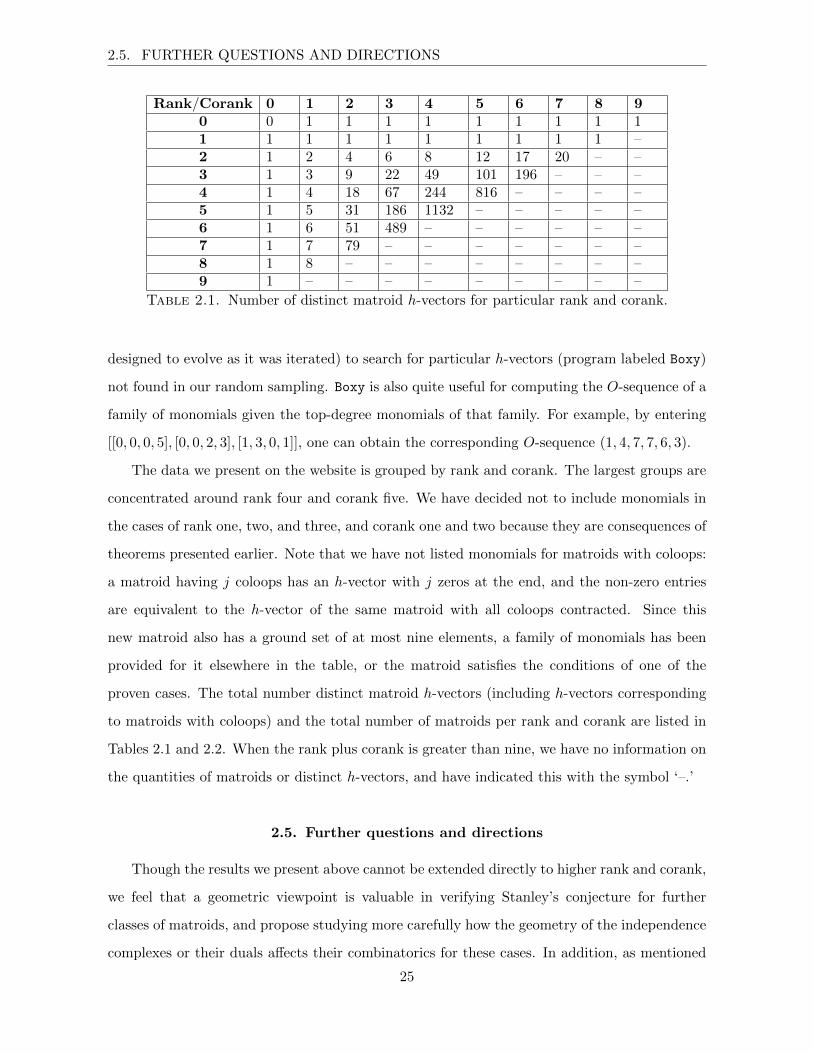
Table 2.2. Total number of matroids, for particular rank and corank.

in the introduction, matroid complexes are one family that satisfies the definition of a PS-ear

decomposable simplicial complex (see [Cha97]). A PS-ear decomposable simplicial complex

is not only conducive to arguments by induction, by definition it satisfies the operations of

deletion and contraction. Can the extra structure given by a PS-ear decomposition enable us

to attack Stanley’s conjecture in a new and effective way?

A further class – also a matroid construction – on which to study the problem of character-

izing f - and h-vectors (or individually, necessary and sufficient conditions) is matroid polytopes.

Definition 2.5.1. Let M be a matroid on n elements. Given a basis B ⊆ {1, . . . , n} of M ,

the indicator vector of B is

eB :=∑i∈B

ei,

where ei is the standard ith unit vector in Rn. Then, the matroid polytope PM is the convex

hull of the set of indicator vectors of the bases of M .

For more on matroid polytopes, see [Zie95]. There has been extensive work already on

the f -vectors of convex polytopes (see for instance [BL93, KK95]), and some of these results

have been extended to matroid polytopes. In general, exploring f -vectors and various related

parameters, such as fatness and complexity [Zie02], is difficult because of the lack of examples;

matroid polytopes however may be constructed inductively, and several algorithmic methods

exist for their construction [BBG09].

26

CHAPTER 3

Polytopal Embeddings of Cayley Graphs

3.1. Not all Cayley graphs are polyhedral

The purpose of this section is to prove the following theorem, and more generally, to show

that not all Cayley graphs can be embedded as the graphs of convex polytopes.

Theorem 3.1.1. The Cayley graph of a minimal presentation of the quaternion group cannot

be embedded as the graph of a convex polytope of any dimension.

To prove this theorem, we study in detail the possible presentations of the quaternion group,

denoted Q8. There are many presentations of Q8, however, the only minimal presentations are

those of the form:

Λ = 〈x, y | x4 = 1, x2 = y2, y−1xy = x−1〉,

where, if Q8 = {±1,±i,±j,±k} and {±i,±j,±k} are the elements of order four, x, y ∈ {±i,

±j, ±k}, and x 6= −y. (Since any non-inverse pair in {±i,±j,±k} generates the entire group,

and we need at least two elements to generate the group, adding further generators would create

redundancies.) All presentations of this type have the same Cayley graph, but for concreteness

we let

Λ = 〈i, j | i4 = 1, i2 = j2, j−1ij = i−1〉.

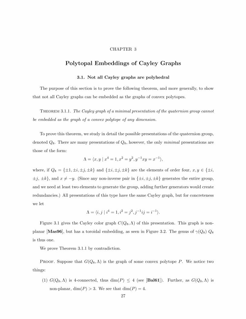
Figure 3.1 gives the Cayley color graph C(Q8,Λ) of this presentation. This graph is non-

planar [Mas96], but has a toroidal embedding, as seen in Figure 3.2. The genus of γ(Q8) Q8

is thus one.

We prove Theorem 3.1.1 by contradiction.

Proof. Suppose that G(Q8,Λ) is the graph of some convex polytope P . We notice two

things:

(1) G(Q8,Λ) is 4-connected, thus dim(P ) ≤ 4 (see [Bal61]). Further, as G(Q8,Λ) is

non-planar, dim(P ) > 3. We see that dim(P ) = 4.

27

3.1. NOT ALL CAYLEY GRAPHS ARE POLYHEDRAL

ijj

−ij −j

1−i

−1 i

Figure 3.1. The Cayley color graph C(Q8,Λ). Dashed lines represent multi-plication on the right by j, and solid lines represent multiplication on the rightby i.

ijj

−ij −j

1−i

−1 i

Figure 3.2. The Cayley color graph C(Q8,Λ), embedded on a torus.

(2) Every vertex of G(Q8,Λ) is of the same degree, thus P is simple. Blind and Mani

[BML87] show that if P is a simple polytope, then its graph G(P ) determines the

entire combinatorial structure of P .

Kalai [Kal88] gave a simpler construction for a simple polytope P given its graph G(P ).

Later, Joswig [Jos00] generalized Kalai’s methods to non-simple polytopes. We will show it

is impossible to complete this construction for G(Q8,Λ), henceforth abbreviated as G. As in

Kalai’s construction, we consider the set of all acyclic orientations of G in order to find the

“good” ones. Good acyclic orientations are given as follows. Let O be an acyclic orientation of

G, and hOk be the number of vertices with in-degree k with respect to O. Define

fO := hO0 + 2hO1 + 4hO2 + 8hO3 + 16hO4 .

28


For all orientations, fO ≥ f , the number of faces of P . An orientation O is good if and only

if fO = f . Of course, we do not know what f is, but if G is indeed the graph of a simple

polytope, a good orientation must exist. Therefore, we must find the minimum fO among all

acyclic orientations O of G. In particular, we will start with a well-chosen orientation O and

corresponding fO, and show that we cannot do better. To this end, consider the orientation of

G given in Figure 3.3.

34

1 2

78

5 6

Figure 3.3. An orientation of G(Q8,Λ), given by the natural ordering of thevertex labels.

We have the in-degrees and corresponding vertices from the ordering in Figure 3.3 in the

following chart:

In-Degree Vertices

0 1

1 2,3

2 4,5

3 6,7

4 8

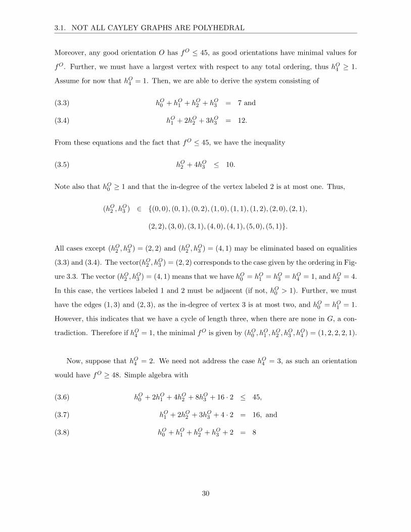
And for this orientation, we have:

fO = 1 · 1 + 2 · 2 + 4 · 2 + 8 · 2 + 16 · 1 = 45.

To see that this is the smallest possible fO, first note that we have the equalities

0 · hO0 + 1 · hO1 + 2 · hO2 + 3 · hO3 + 4 · hO4 = 16, and(3.1)

hO0 + hO1 + hO2 + hO3 + hO4 = 8.(3.2)

29


Moreover, any good orientation O has fO ≤ 45, as good orientations have minimal values for

fO. Further, we must have a largest vertex with respect to any total ordering, thus hO4 ≥ 1.

Assume for now that hO4 = 1. Then, we are able to derive the system consisting of

hO0 + hO1 + hO2 + hO3 = 7 and(3.3)

hO1 + 2hO2 + 3hO3 = 12.(3.4)

From these equations and the fact that fO ≤ 45, we have the inequality

hO2 + 4hO3 ≤ 10.(3.5)

Note also that hO0 ≥ 1 and that the in-degree of the vertex labeled 2 is at most one. Thus,

(hO2 , hO3 ) ∈ {(0, 0), (0, 1), (0, 2), (1, 0), (1, 1), (1, 2), (2, 0), (2, 1),

(2, 2), (3, 0), (3, 1), (4, 0), (4, 1), (5, 0), (5, 1)}.

All cases except (hO2 , hO3 ) = (2, 2) and (hO2 , h

O3 ) = (4, 1) may be eliminated based on equalities

(3.3) and (3.4). The vector(hO2 , hO3 ) = (2, 2) corresponds to the case given by the ordering in Fig-

ure 3.3. The vector (hO2 , hO3 ) = (4, 1) means that we have hO0 = hO1 = hO3 = hO4 = 1, and hO2 = 4.

In this case, the vertices labeled 1 and 2 must be adjacent (if not, hO0 > 1). Further, we must

have the edges (1, 3) and (2, 3), as the in-degree of vertex 3 is at most two, and hO0 = hO1 = 1.

However, this indicates that we have a cycle of length three, when there are none in G, a con-

tradiction. Therefore if hO4 = 1, the minimal fO is given by (hO0 , hO1 , h

O2 , h

O3 , h

O4 ) = (1, 2, 2, 2, 1).

Now, suppose that hO4 = 2. We need not address the case hO4 = 3, as such an orientation

would have fO ≥ 48. Simple algebra with

hO0 + 2hO1 + 4hO2 + 8hO3 + 16 · 2 ≤ 45,(3.6)

hO1 + 2hO2 + 3hO3 + 4 · 2 = 16, and(3.7)

hO0 + hO1 + hO2 + hO3 + 2 = 8(3.8)

30


shows that hO2 + 4hO3 ≤ −1, a contradiction. Therefore, if G is the graph of a simple polytope

P , the orientation pictured above is a good one, and the number of faces of P is 45.

The next question is to find the faces. We have the following from Kalai’s method to recover

the polytope from its graph:

Lemma 3.1.2. An induced, connected, k-regular subgraph H of G is the graph of a k-face of

P (G) if and only if its vertices are initial with respect to some good acyclic orientation O of G.

In the above, P (G) refers to the polytope given by a graph G. Recall that a subgraph H of

an oriented graph G is initial if there are no edges in G directed into H. Let fi be the number

of faces of dimension i. Then,4∑i=0

fi = 45,

and (f0, f1, f2, f3, f4) = (8, 16, ?, ?, 1), so f2 + f3 = 20. However, using the vertex labeling from

above, the set of 2- and 3-faces include (but are not limited to):

1234, 1256, 1278, 1458, 1568,

2-faces 1467, 2358, 2367, 2567, 3456,

3478, 3678, 4578, 5678...

123456, 123478, 123458,

3-faces 123467, 125678, 145678,

235678, 345678...

This is not an exhaustive list of all faces of dimensions two and three, and it already

includes more than 20 faces. We see that G cannot be the graph of a polytope, and no minimal

presentation of Q8 can be embedded as the graph of a convex polytope. �

Remark 3.1.3. The condition of minimality is an important one. If we take the presentation

of Q8:

Λ = 〈i, j, k,−1|(−1)2 = 1, i2 = j2 = k2 = ijk = −1〉,

then G(Q8,Λ) is the complete graph on eight vertices, which can be embedded as the graph of

the 8-simplex.

31

3.2. TWO FAMILIES OF POLYHEDRAL CAYLEY GRAPHS

Note that Q8 is also the smallest example of a group whose Cayley graph cannot be em-

bedded as the graph of a convex polytope of any dimension. All other groups of order less than

or equal to eight are planar.

3.2. Two families of polyhedral Cayley graphs

In this section, we study two families of groups whose Cayley graphs can be embedded as the

graphs of convex polytopes. In the first subsection, we study groups of symmetries of convex,

regular polytopes, and consider the Coxeter complex [Hum90] and a related construction of

Wythoff [Wij18]. In the second, we consider a result of Maschke [Mas96], and extend his

work with a new proof method using graph connectivity and polyhedral techniques.

3.2.1. Groups of symmetries. In this section, we will discuss embeddings of the reflec-

tion presentations of the groups of symmetry of convex, regular polytopes, and our discussion

will lead to a construction that gives the polytopes whose graphs are equal to the Cayley

graphs of the reflection presentations of these groups. We begin with a review of the necessary

background; our exposition follows that of Humphreys [Hum90].

Given a (real) Euclidean space V with a positive definite, symmetric, bilinear form (λ, µ),

a reflection sα is a linear operator on V that sends a vector α ∈ V to −α while fixing the

hyperplane Hα orthogonal to α. We can describe the image of any vector λ ∈ V under sα by

sαλ = λ− 2(λ, α)

(α, α)α.

In some cases, the set of reflections generates a finite group, and one such family is the

groups of symmetries of convex, regular polytopes. For instance, the symmetric group Sn is the

group of symmetries of the standard (n − 1)-dimensional simplex in Rn. The reflections sαij

correspond to the vectors αij = εi − εj , where ε1, . . . , εn are the standard basis vectors of Rn.

(We can think of sαij as a transposition that permutes the ith and jth vertices.)

Let W be a finite reflection group acting on the Euclidean space V . The vectors α corre-

sponding to the reflections sα make up a set of vectors Φ called a root system. More generally,

a root system in V is a set of vectors Φ such that

(R1) Φ ∩ Rα = {α,−α} for all α ∈ Φ, and

(R2) sαΦ = Φ for all α ∈ Φ.

32


In some cases, the root systems are crystallographic, meaning that they satisfy an additional

requirement:

(R3) 2(α,β)(β,β) ∈ Z for all α, β ∈ Φ.

Typically, we start with a root system Φ and then study the group generated by the re-

flections, but given a group of reflections, we can also construct the root system. For crystal-

lographic root systems, the basic strategy is as follows. First, we pick a suitable lattice L in

Rn, and define Φ to be the set of all vectors in L having one or two prescribed lengths (for a

proof that this is a sufficient number of lengths, see [Hum90]). Then, we verify that all scalars

2 (α,β)(β,β) are integers. It then follows that the reflections sα with respect to α ∈ Φ stabilize L and

permute Φ as required. See [Bou68] for more details. We list in Figure 3.4 the convex, regular

polytopes (for dimension d > 1), their associated symmetry groups, and the root systems that

generate these groups. In Figure 3.4, εi is the ith standard basis vector of Rn (where n depends

on the dimension of the polytope). H3 and H4, below, are not crystallographic, and are con-

structed in a different way than described above, see [Hum90, Ste99] for specific details. In

these cases, let:

a = 2 cos(π

5

)=

1 +√

5

2,

b = a2 = a+ 1,

α1 = ε1 + ε2,

α2 =1

2(1− a)(ε1 + ε2 + ε3) +

1

2(1 + a) ε4,

α3 =1

2(ε1 + ε2 + ε3) +

(a− 1

2

)ε4,

α4 =1

2a(ε1 + ε2 + ε3) +

(1

2a− 1

)ε4, and

D4 = {± εi± εj : 1 ≤ i < j ≤ 4}.

Note that polytopes that are polar duals of each other have the same symmetry groups.

While each group of symmetry is completely determined by its root system, we notice that the

root systems are also extremely large and can be difficult to work with. Fortunately, every root

system Φ has a subset Π called a simple system.

33


Polytope Group of Symmetry Root System

m-gon Dm (or I2(m)){

(cos(kπm

), sin

(kπm

)) : 0 ≤ k ≤ 2m

}3-simplex S4 (or A3) {εi− εj : 1 ≤ i 6= j ≤ 4}cube/octahedron B3 {± εi± εj : 1 ≤ i < j ≤ 3}∪

{± εi : 1 ≤ i ≤ 3}dodecahedron/icosahedron H3 {εi : 1 ≤ i ≤ 3}∪

{± ε1±a ε2±b ε3}∪{± ε2±a ε3±b ε1}∪{± ε3±a ε1±b ε2}

4-simplex S5 (or A4) {εi− εj : 1 ≤ i 6= j ≤ 5}4-hypercube/4-cross-polytope B4 {± εi± εj : 1 ≤ i < j ≤ 4}∪

{± εi : 1 ≤ i ≤ 4}24-cell F4 {± εi± εj : 1 ≤ i < j ≤ 4}∪

{± εi : 1 ≤ i ≤ 4}∪{12(± ε1± ε2± ε3± ε4)

}120-cell/600-cell H4 D4 ∪D4α2 ∪D4α3 ∪D4α4

n-simplex Sn+1 (or An) {εi− εj : 1 ≤ i 6= j ≤ n+ 1}n-cube/n-orthoplex Bn {± εi± εj : 1 ≤ i < j ≤ n}∪

{± εi : 1 ≤ i ≤ n}

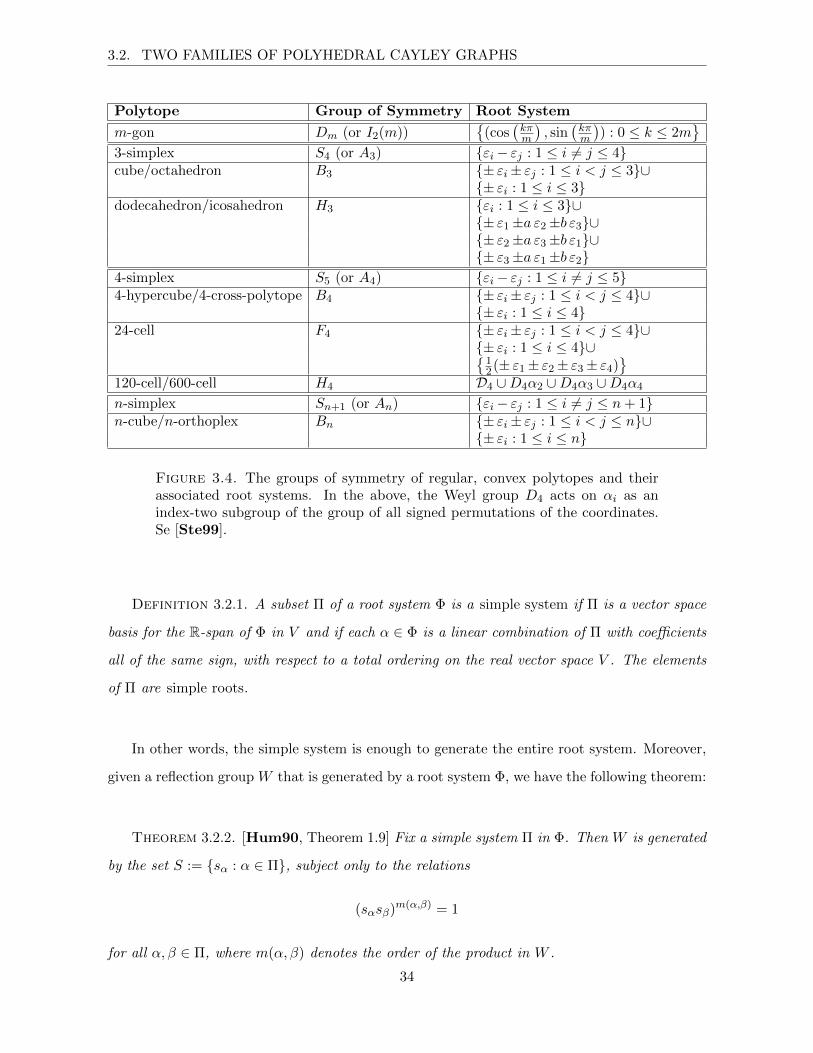
Figure 3.4. The groups of symmetry of regular, convex polytopes and theirassociated root systems. In the above, the Weyl group D4 acts on αi as anindex-two subgroup of the group of all signed permutations of the coordinates.Se [Ste99].

Definition 3.2.1. A subset Π of a root system Φ is a simple system if Π is a vector space

basis for the R-span of Φ in V and if each α ∈ Φ is a linear combination of Π with coefficients

all of the same sign, with respect to a total ordering on the real vector space V . The elements

of Π are simple roots.

In other words, the simple system is enough to generate the entire root system. Moreover,

given a reflection group W that is generated by a root system Φ, we have the following theorem:

Theorem 3.2.2. [Hum90, Theorem 1.9] Fix a simple system Π in Φ. Then W is generated

by the set S := {sα : α ∈ Π}, subject only to the relations

(sαsβ)m(α,β) = 1

for all α, β ∈ Π, where m(α, β) denotes the order of the product in W .

34


Polytope Group of Symmetry Diagram

m-gon Dm (or I2(m))m

3-simplex S4 (or A3)

cube/octahedron BC34

dodecahedron/icosahedron H35

4-simplex S5 (or A4)

4-hypercube/4-cross-polytope BC44

24-cell F44

120-cell/600-cell H45

n-simplex Sn+1 (or An)

n-cube/n-orthoplex BCn4

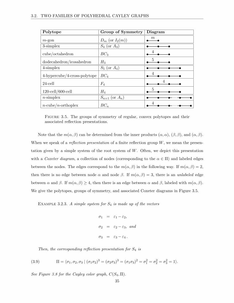
Figure 3.5. The groups of symmetry of regular, convex polytopes and theirassociated reflection presentations.

Note that the m(α, β) can be determined from the inner products (α, α), (β, β), and (α, β).

When we speak of a reflection presentation of a finite reflection group W , we mean the presen-

tation given by a simple system of the root system of W . Often, we depict this presentation

with a Coxeter diagram, a collection of nodes (corresponding to the α ∈ Π) and labeled edges

between the nodes. The edges correspond to the m(α, β) in the following way. If m(α, β) = 2,

then there is no edge between node α and node β. If m(α, β) = 3, there is an unlabeled edge

between α and β. If m(α, β) ≥ 4, then there is an edge between α and β, labeled with m(α, β).

We give the polytopes, groups of symmetry, and associated Coxeter diagrams in Figure 3.5.

Example 3.2.3. A simple system for S4 is made up of the vectors

σ1 = ε1− ε2,

σ2 = ε2− ε3, and

σ3 = ε3− ε4 .

Then, the corresponding reflection presentation for S4 is

(3.9) Π = 〈σ1, σ2, σ3 | (σ1σ2)3 = (σ2σ3)3 = (σ1σ3)2 = σ21 = σ2

2 = σ23 = 1〉.

See Figure 3.8 for the Cayley color graph, C(S4,Π).

35


An important geometric notion associated with each finite reflection group W is its funda-

mental domain.

Definition 3.2.4. Let W be a finite reflection group in a vector space V with a total

ordering, and let Π be a simple system of W with respect to this ordering. Then, the fundamental

domain D is given by

D := {λ ∈ V : (λ, α) ≥ 0 for all α ∈ Π}.

D is a closed, convex cone, and it gets its name from the fact that it represents the funda-

mental domain for the action of W on V — that is, each vector λ ∈ V is conjugate under W to

precisely one point in D (for a proof of this, see [Hum90, Theorem 1.12]). We can partition

D into faces in the following way:

CI := {λ ∈ D : (λ, α) = 0 for all α ∈ ΠI , (λ, α) > 0 for all α ∈ Π \ΠI},

where S is the set of simple reflections of ∆, and I is any subset of S (including the empty set).

Define also

C := {wCI : I ⊆ S and w ∈W}.

If Π spans V , then C partitions V , and we call C the Coxeter complex of W . For more on the

Coxeter complex, see [Hum90]. In addition, when we intersect the elements of C with the unit

sphere in V , we have a simplicial decomposition of the sphere; we denote Sn ∩ C as W. In the

cases of groups of symmetries W of convex, regular polytopes, Π spans Rn, and we have C and

W defined for all the groups we are considering.

The process of partitioning the sphere with reflections of the fundamental domain is also

known as the Wythoff construction (see [Cox73, DDSS08, Max89, MP95, Wij18]). Notice

that each facet of C corresponds to an element w ∈ W , and that two facets share a ridge if

and only if they differ by a simple reflection — that is, one of the generators of W . It is then

clear that the polar dual of W has 1-skeleton equivalent to the Cayley graph of the reflection

presentation of the group of symmetries. We therefore have an embedding of G(W,Π) as the

graph of a convex n-polytope.

Example 3.2.5. As an example, we consider the case of S4. The fundamental domain of

S4 (intersected with the 2-sphere), with respect to the presentation in (3.9), is shown in Figure

3.6. Figure 3.7 then shows W for the case of S4 with presentation (3.9). Taking the polar dual

36


of this complex gives a convex, simple polytope with G(S4,Π) as its graph, drawn in the plane

in Figure 3.8.

π3

π3

σ1

σ3

σ2

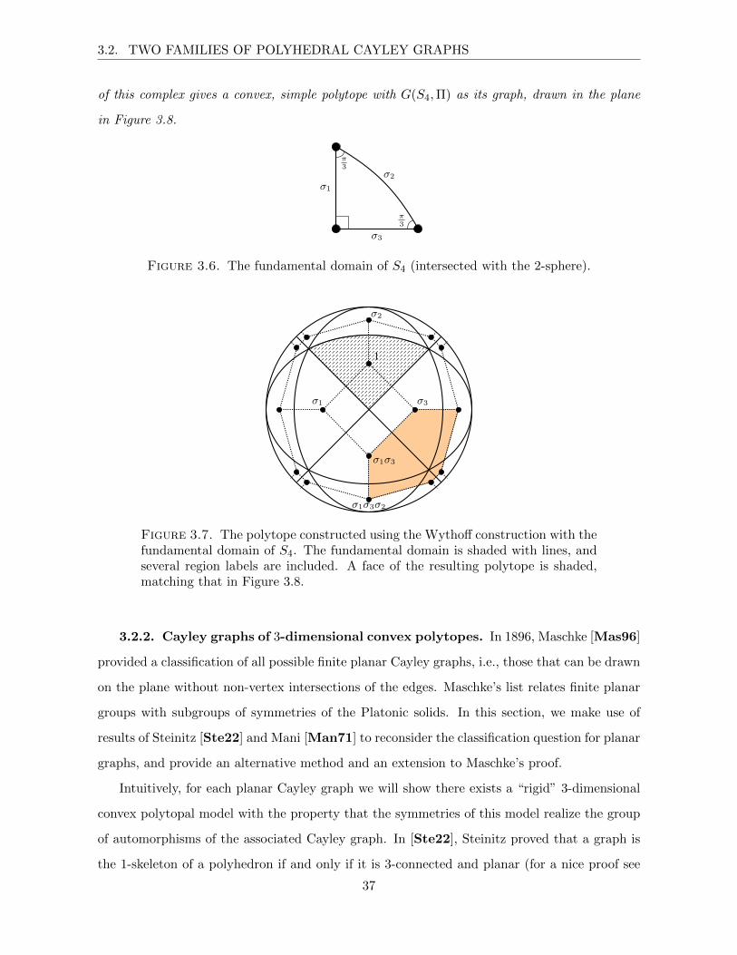
Figure 3.6. The fundamental domain of S4 (intersected with the 2-sphere).

1

σ1

σ1σ3

σ3

σ2

σ1σ3σ2

Figure 3.7. The polytope constructed using the Wythoff construction with thefundamental domain of S4. The fundamental domain is shaded with lines, andseveral region labels are included. A face of the resulting polytope is shaded,matching that in Figure 3.8.

3.2.2. Cayley graphs of 3-dimensional convex polytopes. In 1896, Maschke [Mas96]

provided a classification of all possible finite planar Cayley graphs, i.e., those that can be drawn

on the plane without non-vertex intersections of the edges. Maschke’s list relates finite planar

groups with subgroups of symmetries of the Platonic solids. In this section, we make use of

results of Steinitz [Ste22] and Mani [Man71] to reconsider the classification question for planar

graphs, and provide an alternative method and an extension to Maschke’s proof.

Intuitively, for each planar Cayley graph we will show there exists a “rigid” 3-dimensional

convex polytopal model with the property that the symmetries of this model realize the group

of automorphisms of the associated Cayley graph. In [Ste22], Steinitz proved that a graph is

the 1-skeleton of a polyhedron if and only if it is 3-connected and planar (for a nice proof see

37


σ1σ3σ2

σ1σ3σ2σ1

σ1σ3

σ3

σ3σ2

σ3σ2σ1

1

Figure 3.8. The Cayley color graph of S4 with the presentation in (3.9). Solidlines represent multiplication by σ1, dotted lines represent multiplication by σ2,and dashed lines represent multiplication by σ3.

[Gru03]). A result of Mani [Man71] extends Steinitz’s theorem in a convenient way: every

3-connected, planar graph G is the 1-skeleton of a polyhedron P such that every automorphism

of G is induced by a symmetry of P . Our main goal is to show that if a Cayley graph of the

group Γ embeds in the 2-dimensional sphere, then it acts on the sphere by isometries.

We first give some definitions, well known from graph theory.

Definition 3.2.6. A separator of a graph G = (V,E) is a subset S ⊆ V such that G \ S

is disconnected and has at least two non-empty subgraphs called components. A k-separator is

a separator of cardinality k. A graph is k-connected if there exist no separators of cardinality

less than k.

Definition 3.2.7. An automorphism ϕ of a Cayley color graph C(Γ,Λ) is a permutation

of its vertices such that for all pairs of vertices g1 and g2, and generators h ∈ Γ, ϕ(g1)h = ϕ(g2)

if and only if g1h = g2.

It is well known that the group of automorphisms of a Cayley color graph corresponding to

a group Γ is isomorphic to Γ. A Cayley graph has Γ as a subgroup of its automorphism group,

and Γ acts transitively on the vertices of the graph. We will show that any planar Cayley graph

is either 3-connected or a cycle; we make use of the transitive action of Γ to prove this. First,

we recall the notion of a quadrant.

38


Definition 3.2.8. A graph G is vertex-transitive if for any two vertices v1 and v2 there

exists an automorphism ϕ of G such that ϕ(v1) = ϕ(v2).

Definition 3.2.9. Let A and B be two separators of the graph G. Suppose A separates

G into the components A1 and A2, and B separates G into B1 and B2. The quadrant Qij is

given:

Qij := (Ai ∩B) ∪ (Bj ∩A) ∪ (A ∩B).

For a visualization of this concept, we refer to Figure 3.9. These ideas, including the

following remark, go back to Neumann–Lara [NL89].

B

AA1 A2

B1

B2

Figure 3.9. The graph G, represented by the largest rectangle, with A and Bdrawn as orthogonal strips. Q11 has been shaded.

Remark 3.2.10. Let A and B be two separators of the same connected graph G. If Ai ∩Bj

is non-empty then the quadrant Qij is a separator.

Proof. The proof is simple. Assume without loss of generality that i = j = 1. Further,

assume A1∩B1 is non-empty (see Figure 3.9). Then there are no edges connecting A1∩B1 and

B2 because B is a separator. Similarly, there are no edges connecting A1 ∩ B1 and A2. Thus,

Q11 separates A1 ∩B1 and A2 ∪B2. �

Now we are able to prove the following result:

Proposition 3.2.11. Let G be a connected, vertex-transitive graph with minimum degree

at least two. Then G is a cycle or a 3-connected graph.

Proof. First, note that G must be at least 2-connected, as it is vertex-transitive with

minimum degree at least two. Second, we assume that G 6= K3 (the proposition holds in this

39


case, but there are not enough vertices for our argument). Suppose G is not 3-connected.

Let A = {x, y} be a 2-separator with components A1 and A2 such that A1 is minimal among

all possible components of 2-separators in G. Since G is vertex-transitive, there exists an

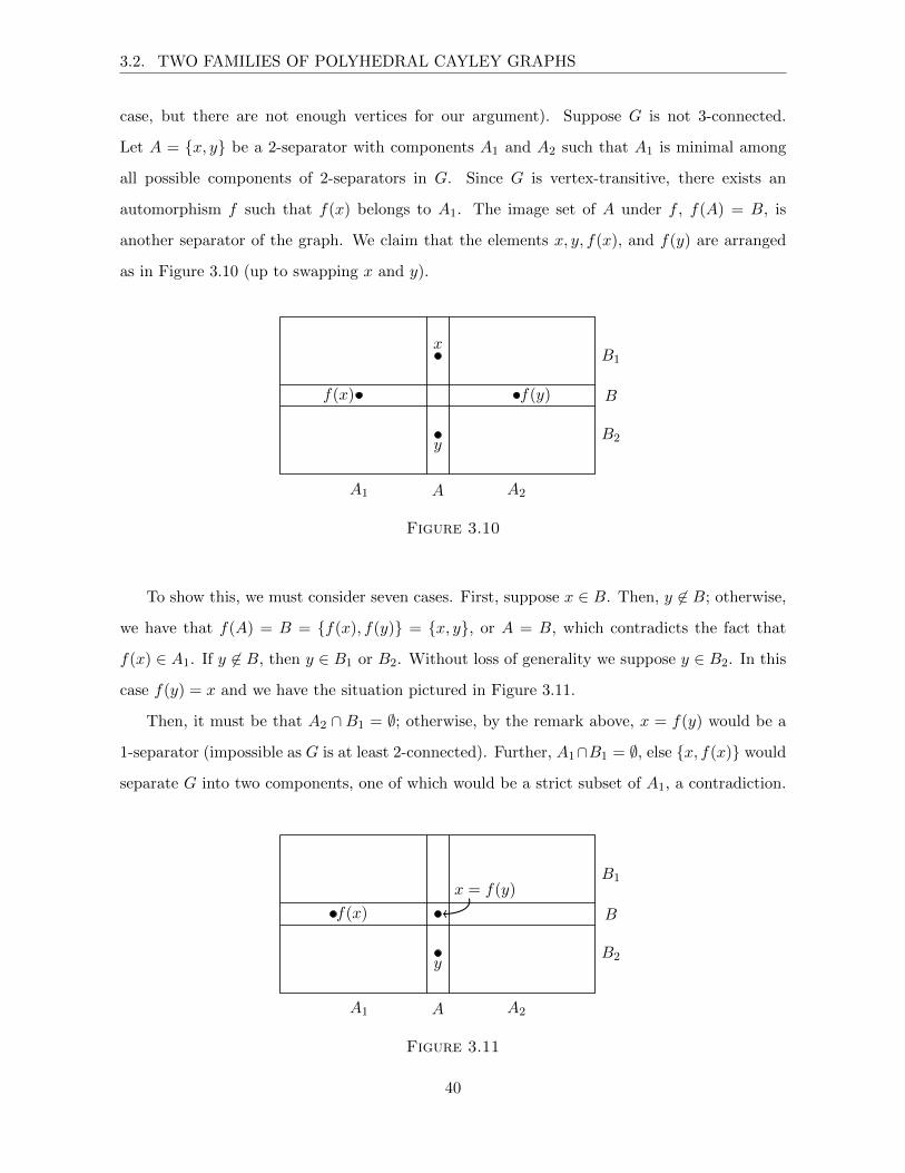
automorphism f such that f(x) belongs to A1. The image set of A under f , f(A) = B, is

another separator of the graph. We claim that the elements x, y, f(x), and f(y) are arranged

as in Figure 3.10 (up to swapping x and y).

B

AA1 A2

B1

B2

f(y)f(x)

x

y

Figure 3.10

To show this, we must consider seven cases. First, suppose x ∈ B. Then, y 6∈ B; otherwise,

we have that f(A) = B = {f(x), f(y)} = {x, y}, or A = B, which contradicts the fact that

f(x) ∈ A1. If y 6∈ B, then y ∈ B1 or B2. Without loss of generality we suppose y ∈ B2. In this

case f(y) = x and we have the situation pictured in Figure 3.11.

Then, it must be that A2 ∩ B1 = ∅; otherwise, by the remark above, x = f(y) would be a

1-separator (impossible as G is at least 2-connected). Further, A1∩B1 = ∅, else {x, f(x)} would

separate G into two components, one of which would be a strict subset of A1, a contradiction.

B

AA1 A2

B1

B2

f(x)

x = f(y)

y

Figure 3.11

40


However, then B1 = ∅, contradicting the fact that B is a separator. Therefore, x must be in

B1 or B2.

Now, we claim that x and y are separated by B. Suppose not. Then, we have one of the

situations pictured in Figures 3.12, 3.13, and 3.14.

B

AA1 A2

B1

B2

f(x)

y = f(y)

x

Figure 3.12

B

AA1 A2

B1

B2

f(y)f(x)

x

y

Figure 3.13

B

AA1 A2

B1

B2

f(y)f(x)

x

y

Figure 3.14

41


In Figure 3.12, we see that A2 ∩ B2 must be empty (otherwise, y would be a 1-separator),

and A1 ∩ B2 must be empty (otherwise, we would have a separator with a component strictly

smaller than A1). This implies that B is not a separator, a contradiction. In Figures 3.13 and

3.14, similar arguments may be used. Therefore, x and y must be separated by B. Finally, we

claim that f(y) is a point in A2. Suppose that f(y) ∈ A1, as shown in Figure 3.15.

B

AA1 A2

B1

B2

f(y)f(x)

x

y

Figure 3.15

It follows from our remark that A2 ∩B2 and A2 ∩B1 are empty. Otherwise the quadrants

Q21 and Q22 would be separators of G, but these quadrants have only one point, thus this

point is a 1-separator of the graph. Thus, A2 is empty, contradicting the fact that A is a

separator. Further, f(y) is not in A, otherwise f(x) = x or f(x) = y, contradicting the fact

that B separates x and y. Therefore, f(y) ∈ A2, and we must have the arrangement in Figure

3.10.

In this case, A1 ∩ B1 and A1 ∩ B2 must be empty. Otherwise, the quadrants Q11 and Q12

would be separators, but removing either quadrant would leave a component with fewer vertices

than A1. Therefore, f(x) is the only vertex in A1, and it must be adjacent to both x and y, as

every vertex has degree at least two. f(x) is thus a vertex of degree exactly two, which implies

that G is regular of degree two. Since G is connected, G must be a cycle. Finally, Steinitz’s

theorem says that a planar graph is the graph of a 3-polytope if and only if it is 3-connected.

Proposition 3.2.11 then follows. �

Now we can prove the main theorem of this section.

Theorem 3.2.12. Let Γ be a finite group with a minimal set of generators and relations Λ.

The associated Cayley graph is the graph of a 3-dimensional polytope if and only if Γ is a finite

group of isometries in 3-dimensional space.

42


Proof. G(Γ,Λ) satisfies the hypotheses of Proposition 3.2.11. If G(Γ,Λ) is a cycle, then

Γ is a dihedral group or a cyclic group. Both groups have an isometric action on the sphere as

symmetries of an n-dihedron. In the case that G(Γ,Λ) is 3-connected, Mani’s result [Man71]

gives the required action. See [Tuc83] for a different view of the theorem. �


We have found one example of a Cayley graph that does not appear as the graph of a convex

d-polytope. It is therefore natural to ask for further examples of groups whose Cayley graphs

do not embed in this way.

Question 3.3.1. Are there (infinite) families of groups whose minimal presentations cannot

be embedded as the graphs of convex d-polytopes?

One possible family is the set of generalized quaternion groups, of which Q8 is the small-

est member. More generally, we propose to explore group-theoretic characterizations of non-

embeddability.

Question 3.3.2. Can we use group theory to characterize the embeddability of Cayley

graphs? Can we characterize subgroups that in some sense “block” the embedding of the Cayley

graphs? Or can we show that there exist no such subgroups?

We can also approach the problem of embedding Cayley graphs from a graph-theoretic

standpoint.

Question 3.3.3. Are there forbidden minor characterizations for the embeddability of Cay-

ley graphs, as in the case of Kuratowski’s theorem (Theorem 1.0.1)?

Cayley graphs have many special properties that could be used in answering this question.

For example, Cayley graphs are vertex-transitive, and could thus only be the graphs of sim-

ple polytopes. Studying these questions is additionally of interest for the purpose of better

understanding the 1-skeletons of convex polytopes.

The Coxeter complex and the Wythoff construction described above are further sources of

questions.

Question 3.3.4. Can we design other constructions that give d-polytopes with graphs equal

to Cayley graphs?

43

CHAPTER 4

Flows on Simplicial Complexes

4.1. Structure of the boundary matrices of simplicial complexes

To begin, we examine the structure of the boundary matrix ∂∆ of a simplicial complex ∆,

given a certain ordering of the rows and columns. Before stating our first lemma, we recall a

few definitions.

Definition 4.1.1. Let ∆ be a simplicial complex, and let F be a face of ∆. Then, the link

of F in ∆, denoted lk∆(F ), is given by

lk∆(F ) := {G ∈ ∆ : G ∩ F = ∅, G ∪ F ∈ ∆}.

Definition 4.1.2. Let ∆ be a simplicial complex, and let F be a face of ∆. Then, the

deletion of F from ∆, denoted ∆− F , is given by

∆− F := {G ∈ ∆ : G ∩ F = ∅}.

Definition 4.1.3. A simplicial cone is a pure simplicial complex ∆ with a vertex v such

that v is contained in every facet of ∆.

Note that the class of simplicial complexes is closed under the operations of taking the link

of a face and deleting a face. We can now state the following.

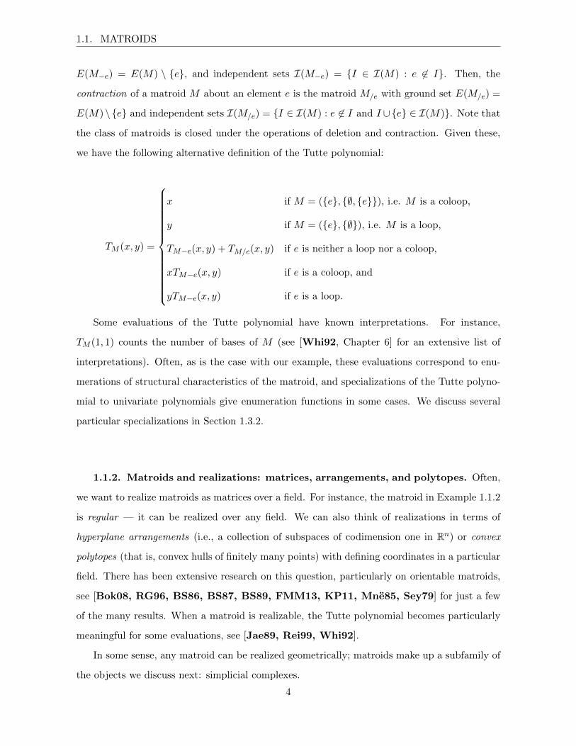
Lemma 4.1.4. Let ∆ be a simplicial complex of dimension d that is not a cone, with ordering

v1 < v2 < · · · < vn on the vertices. Arrange the rows (indexed by the ridges of ∆) and columns

(indexed by the facets of ∆) of ∂∆ in the following way:

(1) Let all ridges containing the vertex vn come first, and order them lexicographically,

according to the ordering on the vertices of ∆.

(2) Let all ridges in lk∆(vn) be next, ordered lexicographically.

(3) Order the remaining ridges lexicographically.

(4) Let all facets containing vn come first, and order them lexicographically.

44

4.1. STRUCTURE OF THE BOUNDARY MATRICES OF SIMPLICIAL COMPLEXES

∂∆ = (−I)d

(c)

∂(lk∆(vn))

(a)

0

(b)

∂(∆− vn)

(e)

0(d)

Figure 4.1. The matrix structure described in Lemma 4.1.4.

(5) Order the remaining facets (those that do not contain vn) lexicographically.

Under these conditions, the boundary matrix takes the form given by Figure 4.1.

Proof. We will verify the matrix blocks individually.

(a) This submatrix is equivalent to the boundary matrix of lk∆(vn). Intuitively, the facets of

the link of a vertex are the faces F \vn, where F is a facet of ∆ containing vn. Similarly, the

ridges of lk∆(vn) are the ridges R \ vn, where R is a ridge of ∆ containing vn. These ridges

R and facets F are precisely the rows and columns of (a). Then, since we are removing the

lexicographically largest element from each ridge and facet, we do not affect the signs of

ridges in the boundary map, and the entries of this submatrix are thus identical to those

of ∂(lk∆(vn)).

(b) This block contains only zeros as the rows all contain vn, but the columns do not.

(c) This block is (−I)d, where d is the dimension of ∆. The ridges of this region are precisely

the facets of this region with vn removed, and we have ordered them both lexicographically.

The sign depends on the dimension of ∆ as we are removing the dth element, so the sign of

each ridge is (−1)d.

(d) This block is 0 because we have already listed all ridges that contain vn or are in the link

of vn. Therefore, these ridges cannot be contained in any facet containing vn. We can also

think of this block as containing the ridges that have a vertex vi that is parallel to vn, so

there exists no facet containing vi and vn.

45


(e) This block corresponds to the boundary matrix of the deletion of vn in ∆, ∂(∆− vn). The

facets of ∆− vn are the facets of ∆ that do not contain vn, and the ridges of ∆− vn are the

ridges of ∆ that do not contain vn. This corresponds precisely to the rows and columns of

(e), and since we do not affect the parity of the vertices in the facets, the signs remain the

same. �

See Figure 4.2 for an example of Lemma 4.1.4.

124 134 234 012 013 023 12314 −1 −1 0 0 0 0 024 1 0 −1 0 0 0 034 0 1 1 0 0 0 012 1 0 0 0 1 0 −113 0 1 0 0 1 0 −123 0 0 1 0 0 1 101 0 0 0 1 1 0 002 0 0 0 −1 0 1 003 0 0 0 0 −1 −1 0

(a) Boundary matrix of 4.2b, with regions (a) – (e)blocked off.

1 2

3

4

0

(b) A triangular bipyramid onfive vertices.

Figure 4.2

4.1.1. Flows on simplicial cones. If ∆ is a cone over a vertex v, then we have a variation

of Lemma 4.1.4. Note that if ∆ is a cone over v, then every ridge either contains v, or is in the

link of v. Moreover, by definition, there are no facets that do not contain v.

Lemma 4.1.5. Let ∆ be a pure simplicial complex that is a cone over a vertex v, and order

the vertices v0, v1, . . . , vn so that v = vn is the largest. Arrange the rows (indexed by ridges of

∆) and columns (indexed by facets of ∆) of ∂∆ in the following way:

(1) Let all ridges containing the vertex vn come first, and order them lexicographically.

(2) Order the remaining ridges lexicographically (these are all the ridges in lk∆(vn)).

(3) Order the facets lexicographically (all contain vn).

Under these conditions, the boundary matrix takes the form given by Figure 4.3.

Proof. Let ∆ be a pure simplicial cone over a vertex v and order the vertices v0, v1, . . . , vn

so that v = vn is the largest. In the boundary matrix described in the statement of the lemma,

we only have two regions (there are two types of ridges and one type of facet): region (i) in

46


∂∆ =

(−I)d

(ii)

∂(lk∆(vn)) =

∂(∆− vn)

(i)

Figure 4.3. The boundary matrix of a simplicial cone, as described in Lemma 4.1.5.

Figure 4.3 corresponds to region (a) in Figure 4.2, and region (ii) corresponds to region (c). The

proofs that region (i) is equivalent to ∂(lk∆(vn)) and that region (ii) is (−I)d are identical to the

proofs for regions (a) and (c); we omit them here. We need only show that ∆− vn = lk∆(vn),

but this is immediate from their definitions:

∆− vn = {F ∈ ∆ : vn 6∈ F}

= {F ∈ ∆ : F ∩ vn = ∅}

= {F ∈ ∆ : F ∩ vn = ∅, F ∪ vn ∈ ∆}

= lk∆(vn).

The third equality follows because vn is in every maximal face, thus, if vn 6∈ F ∈ ∆, then

(F ∪ vn) ∈ ∆. �

See Figure 4.4 for an example of this matrix and corresponding simplicial cone.

124 134 23414 −1 −1 024 1 0 −134 0 1 112 1 0 013 0 1 014 0 0 1

(a) Boundary matrix of 4.4b, with regions (i) and(ii) blocked off.

4

2

3

1

(b) A triangular cone on fourvertices.

Figure 4.4

47

4.2. THE NUMBER OF NOWHERE-ZERO ZQ-FLOWS ON A SIMPLICIAL COMPLEX

Lemma 4.1.6. Let ∆ be a pure simplicial complex that is a cone over a vertex v. Then ∆

has no nontrivial Zq-flows.

Proof. Order the vertices v0, v1, . . . , vn so that v = vn is the largest. Since ∆ is a cone over

vn, we have a boundary matrix of the form in Figure 4.3. Notice that (−I)d extends through

all columns. Therefore, ker(∂∆) ⊆ ker((−I)d) = {0}, and there exist only trivial flows. �

4.2. The number of nowhere-zero Zq-flows on a simplicial complex

To study the question of counting nowhere-zero flows, we will use matroid theory, in par-

ticular a generalization of the Tutte polynomial given in [OW79], called a Tutte-Grothendieck

invariant. This generalization allows the recursive definition to include coefficients in the case

that e is neither a loop nor a coloop.

Definition 4.2.1. A function on the class of matroids is a generalized Tutte–Grothendieck

invariant if it is a function f from the class of matroids to a field F such that for all matroids

M and N , f(M) = f(N) whenever M ∼= N , and for all e ∈ E(M),

f(M) =

σf(M−e) + τf(M/e) if e is neither a loop nor a coloop, and

f(M(e))f(M−e) otherwise,

where M(e) is the matroid consisting of the single element e, and σ and τ are nonzero elements

of F.

For more background on Tutte–Grothendieck invariants, see [Whi92, Chapter 6]. In the

following, we will denote by C the matroid consisting of a single coloop and by L the matroid

consisting of a single loop. In order to relate the invariant we find in the proof of Theorem 4.2.3

to the Tutte polynomial, we will use the following fact [OW79, Theorem 6.2.6]:

Theorem 4.2.2. Let σ and τ be nonzero elements of a field F. Then there is a unique

function t′ from the class of matroids into the polynomial ring F[x, y] having the following

properties:

(i) t′C(x, y) = x and t′L(x, y) = y.

(ii) If e is an element of the matroid M and e is neither a loop nor a coloop, then

t′M (x, y) = σ t′M−e(x, y) + τ t′M/e(x, y).

48


(iii) If e is a loop or a coloop of the matroid M , then t′M (x, y) = t′M(e)(x, y) t′M−e(x, y).

Furthermore, this function t′ is given by t′M (x, y) = σ|E|−rk(E)τ rk(E) TM (xτ ,yσ ) .

Finally, recall that any matrix may be realized as a matroid M by taking E(M) to be the

list of columns, and I(M) to be the linearly independent subsets of columns. If y ∈ Z|E(M)|q ,

then the support of y is supp(y) := {e ∈ E(M) : ye 6= 0}. We will now prove the following:

Theorem 4.2.3. Let q be a sufficiently large prime number, and let ∆ be a simplicial complex

of dimension d. Then the number φ∆(q) of nowhere-zero Zq-flows on ∆ is a polynomial in q of

degree βd(∆) = dimQ(Hd(∆,Q)).

Proof. Let ∆ be a pure simplicial complex, and ∂∆ be the boundary matrix associated

with ∆. Let M be the matroid given by the columns of ∂∆, and denote the ground set as E.

For convenience, and by a slight abuse of notation, we will use M to denote both the matroid

and the matrix representing it.

First, we claim that

TM (0, 1− q) = |{y ∈ ker(M) mod q : supp(y) = E}|

for any prime q that is sufficiently large. We show this by proving that the function

gM (q) := |{y ∈ ker(M) mod q : supp(y) = E}|

is a generalized Tutte-Grothendieck invariant with σ = −1 and τ = 1. The matrix for the single

coloop C is a single (linearly independent) vector, thus gC(q) = 0. The matrix for the single

loop L is the zero vector, so gL(q) = q − 1. Thus gM (q) is well-defined if |E| = 1.

Assume g is well-defined for |E| < n, and let |E| = n. Let e ∈ E, and suppose that e is

neither a loop nor a coloop. In the case of a matroid corresponding to a vector configuration

(as is the case with the boundary matrix), contraction models quotients: let V be the vector

space given by E (the columns of the boundary matrix), and let π : V → V/Ve be the canon-

ical quotient map, where Ve is the vector space spanned by the column vector e. Then, the

contracted matroid M/e is the matroid associated with the vector configuration {π(v)}v∈E\e in

49


the quotient space V/Ve. Let

W := {y ∈ ker(M) : supp(y) = E},

X := {y ∈ ker(M − e) : supp(y) = E \ e}, and

Z := {y ∈ ker(M/e) : supp(y) = E \ e}.

We see that W ∩ X = ∅. By linearity of π, we have that W ∪ X ⊂ Z. Now, suppose we

have y ∈ Z. This is a linear combination of all vectors in E \ e that equals a scalar α ∈ Zq

times e (that is, a linear combination equivalent to zero in the quotient space). If α 6= 0, then

(y, α) ∈W . If α = 0, y ∈ X. Therefore

gM (q) = gM/e(q)− gM−e(q) .

If e is a loop (a column of zeros), then e may be assigned any of the q − 1 nonzero values

of Zq. Thus, for loops

gM (q) = (q − 1) gM−e(q)

= gL(q) gM−e(q) .

Finally, suppose e is a coloop. Then every maximally independent set of columns contains

e, and we can use row operations to rewrite M so that the column corresponding to e has

precisely one nonzero element, and this element is also the only nonzero element in its row.

Therefore the entry of a vector y ∈ ker(M) corresponding to e must be 0 for all y ∈ ker(M),

and

gM (q) = 0 · gM−e(q)

= gI(q) gM−e(q) .

Thus gM (q) is well-defined and a generalized Tutte–Grothendieck invariant. We showed the

cases for |E| = 1 above, so we see that by Theorem 4.2.2

gM (q) = t′M (0, q − 1) = (−1)|E|−rk(E)TM (0, 1− q),

50


and so

TM (0, 1− q) = |{y ∈ ker(M) mod q : supp(y) = E}| .

It follows that the number of nowhere-zero Zq-flows on a simplicial complex ∆ is equal to

TM (0, 1− q) and hence is a polynomial in q. Using the definition of the Tutte polynomial, we

see that the degree of this polynomial, in terms of the matroid, is |E| − rk(M). From linear

algebra, we know that

|E| = dim(rk(M)) + dim(ker(M)) = rk(M) + dim(ker(M)) ,

so |E| − rk(M) = dim(ker(M)). But dim(ker(M)) is just the dimension of the top rational

homology of ∆, denoted dimQ(Hd(∆;Q)). By definition, this is βd(∆), where d = dim(∆). �

Remark 4.2.4. We require that q be prime as otherwise V and Ve would be modules, rather

than vector spaces. Requiring that q be sufficiently large ensures that the matrices reduce cor-

rectly over Fq; that is, we require that the linear (in)dependencies of ∂∆ are the same over Q as

they are over Fq. For a simplicial complex of dimension d, a sufficient bound would be q greater

than (d + 1)d+12 , or q greater than the absolute value of the determinant of every submatrix,

though these are not necessarily tight.

4.2.1. Quasipolynomiality of φ∆(q). In this section, we prove the following:

Theorem 4.2.5. The number φ∆(q) of nowhere-zero Zq-flows on ∆ is a quasipolynomial in

q. Furthermore, there exists a polynomial p(x) such that φ∆(k) = p(k) for all integers k that

are relatively prime to the period of φ∆(q). In addition, there are examples where the periodicity

of the quasipolynomial is strictly larger than one.

Proof. Recall that rational polytopes are sets of the form{x ∈ Rd : Ax ≤ b

}for some

integral matrix A and integral vector b. Then, by definition, the flow counting function φ∆(q)

counts the integer lattice points x = (x1, x2, . . . , xn) (where n is the number of facets of ∆)

that satisfy

0 < xj < q and ∂∆(x) = mq for some m ∈ Z .

(Note that we only need to consider finitely many m.) Therefore, to compute φ∆(q), we count

the lattice points in a collection of rational polytopes. By Ehrhart’s theorem (Theorem 1.3.11)

φ∆(q) is a sum of Ehrhart quasipolynomials and thus also a quasipolynomial in q. Now, suppose

51


that φ∆(q) has period p. By Dirichlet’s theorem, there exist infinitely many primes of the form

j + kp for gcd(j, p) = 1 and k ∈ Z≥0, and thus φ∆(j + kp) agrees with the polynomial found in

Theorem 4.2.3 for those j with gcd(j, p) = 1. �

We remark that a setup similar to the one in our proof was used in [BS12] to study flow

polynomials of graphs from the perspective of Ehrhart theory.

Given that the number of nowhere-zero Zq-flows on a graph is a polynomial in q, it is natural

to ask whether the same is true for all simplicial complexes. Interestingly, this is not always

the case. Consider the case of the Klein bottle, K. We have the following top homologies for

K:

H2(K,Zq) =

0 if q is odd, and

Z2 if q is even.

Therefore, the number of nowhere-zero Zq-flows on K is given by a quasipolynomial of period

2:

φK(q) =

0 if q is odd, and

1 if q is even.

4.2.2. Calculating φ∆(q): an example. Consider the triangular bipyramid ∆ with ver-

tex set {0, 1, 2, 3, 4} and facets {012, 013, 023, 123, 124, 134, 234}. Then ∂∆ is given by Figure

4.2a. The kernel for this matrix is generated by

{(1,−1, 1, 0, 0, 0,−1)T , (0, 0, 0,−1, 1,−1, 1)T }.

Thus, any nowhere-zero Zq-flow will have the form (a,−a, a,−b, b,−b, b − a)T where a, b ∈ Zq

and a 6= b. We have q − 1 nonzero choices for a, and q − 2 nonzero choices for b. We see that

φ∆(q) = (q−1)(q−2). For primes p > 1 (one being the maximum over all absolute values of all

subdeterminants of ∂∆), we may also compute φ∆(q) = TM (0, 1− q), where M is the matroid

given by ∂M , as

TM (0, 1− q) =∑S⊆E

(−1)rk(M)−rk(S)(−q)|S|−rk(S)

= q2 − 3q + 2

= (q − 1)(q − 2).

52

4.3. THE PERIOD OF THE FLOW QUASIPOLYNOMIAL

4.3. The period of the flow quasipolynomial

Tutte’s polynomiality result for the number of nowhere-zero flows on graphs also follows

from the fact that the boundary matrix of every graph is totally unimodular, that is, every

subdeterminant is −1, 0, or 1. The total unimodularity of the boundary matrix guarantees that

the flow polytope has integral vertices (see for instance [BS13, Chapter 10.1]), which in turn

implies that the period of the Ehrhart quasipolynomial is one.

With the example of the Klein bottle above, we have already established that the flow

quasipolynomial does in some cases have period strictly greater than one. It is natural, then,

to ask if there are subclasses of simplicial complexes which have flow quasipolynomials with

period equal to one. In particular, we hoped to use the following result of Dey, Hirani, and

Krishnamoorthy to establish total unimodularity of boundary matrices for certain subclasses

of simplicial complexes.

Theorem 4.3.1. [DHK11, Theorem 5.2] For a finite simplicial complex ∆ of dimension

greater than d − 1, the d-dimensional boundary matrix ∂∆ is totally unimodular if and only

if Hd−1(L,L0) is torsion-free for all pure subcomplexes L0, L in ∆ of dimensions d − 1 and d

respectively, where L0 ⊂ L.

(For more information on homology and torsion, see [Hat02, Chapter 2].) In other words,

we can rephrase our original combinatorial question as a topological question, which allows

us to use the language and tools of topology to address the total unimodularity of boundary

matrices. With this in mind, we examined the case of CED complexes. Interestingly, we

found examples demonstrating that CED complexes do not in general have totally unimodular

boundary matrices, nor do they have flow quasipolynomials with period necessarily equal to

one. We give two examples. First, we take the triangulated rectangular bipyramid given in

Figure 4.5.

Consider the submatrix of the boundary matrix that corresponds to facets {124, 126, 236,

346, 345, 145} and ridges {12, 26, 36, 34, 45, 14} of the simplicial complex in Figure 4.5, written

out in Figure 4.6.

The determinant of this submatrix is two — hence the boundary matrix is not totally

unimodular. In the language of [DHK11], the facets in this subcomplex correspond to a

Mobius band embedded in the simplicial complex. There are two other items of note: first, this

53


1

2 3

4

5

6

Figure 4.5. A triangulated rectangular bipyramid on six vertices.

124 126 236 346 345 14512 1 1 0 0 0 026 0 1 0 −1 0 036 0 0 0 1 0 −134 0 0 0 0 1 145 0 0 1 0 1 014 −1 0 1 0 0 0

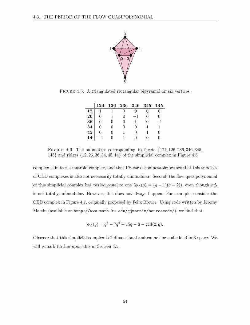
Figure 4.6. The submatrix corresponding to facets {124, 126, 236, 346, 345,145} and ridges {12, 26, 36, 34, 45, 14} of the simplicial complex in Figure 4.5.

complex is in fact a matroid complex, and thus PS-ear decomposable; we see that this subclass

of CED complexes is also not necessarily totally unimodular. Second, the flow quasipolynomial

of this simplicial complex has period equal to one (φ∆(q) = (q − 1)(q − 2)), even though ∂∆

is not totally unimodular. However, this does not always happen. For example, consider the

CED complex in Figure 4.7, originally proposed by Felix Breuer. Using code written by Jeremy

Martin (available at http://www.math.ku.edu/~jmartin/sourcecode/), we find that

φ∆(q) = q3 − 7q2 + 15q − 8− gcd(2, q).

Observe that this simplicial complex is 2-dimensional and cannot be embedded in 3-space. We

will remark further upon this in Section 4.5.

54


1

2

3

4

5

6

12

4

5

7

82

6 5

3

4

7

1

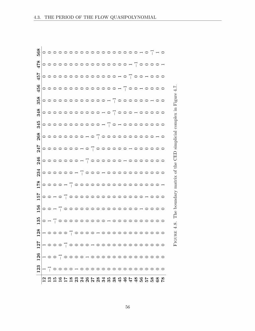
Figure 4.7. A CED complex that is not totally unimodular and has periodequal to 2. Vertices with the same labels are identified, as are edges betweentwo identified vertices. The boundary matrix is given in Figure 4.8.

55


123

126

127

128

135

156

157

178

234

246

247

268

345

348

358

456

457

478

568

12

11

11

00

00

00

00

00

00

00

013−

10

00

10

00

00

00

00

00

00

015

00

00

−1

11

00

00

00

00

00

00

16

0−

10

00

−1

00

00

00

00

00

00

017

00

−1

00

0−

11

00

00

00

00

00

018

00

0−

10

00

−1

00

00

00

00

00

023

10

00

00

00

10

00

00

00

00

024

00

00

00

00

−1

11

00

00

00

00

26

01

00

00

00

0−

10

10

00

00

00

27

00

10

00

00

00

−1

00

00

00

00

28

00

01

00

00

00

0−

10

00

00

00

34

00

00

00

00

10

00

11

00

00

035

00

00

10

00

00

00

−1

01

00

00

38

00

00

00

00

00

00

0−

1−

10

00

045

00

00

00

00

00

00

10

01

10

046

00

00

00

00

01

00

00

0−

10

00

47

00

00

00

00

00

10

00

00

−1

10

48

00

00

00

00

00

00

01

00

0−

10

56

00

00

01

00

00

00

00

01

00

157

00

00

00

10

00

00

00

00

10

058

00

00

00

00

00

00

00

10

00

−1

68

00

00

00

00

00

01

00

00

00

178

00

00

00

01

00

00

00

00

01

0

Figure4.8.

Th

eb

oun

dar

ym

atri

xof

the

CE

Dsi

mpli

cial

com

ple

xin

Fig

ure

4.7

.

56

4.4. FLOWS ON TRIANGULATIONS OF MANIFOLDS

4.4. Flows on triangulations of manifolds

In this section, we prove the following:

Proposition 4.4.1. Let ∆ be a triangulation of a manifold. Then

φ∆(q) =

0 if ∆ has boundary,

q − 1 if ∆ is without boundary, Z-orientable,

0 if ∆ is without boundary, non-Z-orientable, and q is even,

1 if ∆ is without boundary, non-Z-orientable, and q is odd.

Proof. Consider a pure simplicial complex that is a triangulation of a connected manifold.

First, if the manifold has boundary, then there exists at least one ridge that belongs to only

one facet. Since this corresponds to a row in its boundary matrix with precisely one nonzero

entry, any vector in the kernel must have a zero in the coordinate corresponding to the facet

containing this ridge. Therefore, manifolds with boundary do not admit nowhere-zero flows.

If a triangulated manifold N is without boundary, then every ridge belongs to precisely two

facets. This corresponds to every row of ∂N having exactly two nonzero entries. Therefore,

since our manifold is connected, in a valid flow the assigned value of any facet is equal or

opposite mod q to the assigned value of any other facet. It follows that every flow that is

somewhere zero must in fact be trivial.

It is known (see, for instance [Hat02, Chapter 3.3, Theorem 3.26]) that the top homology

of a closed, connected, and Z-orientable manifold N of dimension n is

Hn(N,Z) ∼= Z.

In terms of boundary matrices, this means that the kernel of the boundary matrix has rank

one, since there are no simplices of dimension higher than n. By our comment above, we see

that the non-trivial elements of the kernel must be nowhere-zero, and all entries are ±a ∈ Z. It

is then easy to see that triangulations of closed, connected, orientable manifolds have precisely

q − 1 nowhere-zero Zq-flows.

If M is non-orientable, connected, and of dimension n, then we know (again, see [Hat02])

that the top homology is

57


Hn(M,Γ) ∼=

0 if Γ = Z,

0 if Γ = Z2k+1, and

Z2 if Γ = Z2.

Therefore, if q is odd, we have no non-zero Zq-flows. However, as every manifold is orientable

over Z2, and since every row of the boundary matrix has precisely two nonzero entries, the vector

with all entries equal to k is a nowhere-zero Z2k-flow on M (in fact, the only one). �


We have shown above that not all simplicial complexes have flow quasipolynomials that

are true polynomials. However, it is still natural to ask for which complexes φ∆(q) is a poly-

nomial. Early experiments suggest that matroid and shifted complexes may be examples of

such subclasses. Moreover, for the particular case of CED complexes, we propose the following

questions:

Question 4.5.1. What topological/geometric conditions on a simplicial complex ∆ are nec-

essary for φ∆(q) to have period equal to one?

Question 4.5.2. What topological/geometric conditions on a simplicial complex ∆ are suf-

ficient for φ∆(q) to have period equal to one?

We also propose to find topological properties of simplicial complexes that guarantee that

the flow quasipolynomial has period strictly greater than one. One possible condition – inspired

by [DHK11], the Klein bottle example, and our second CED example – involves the ability to

embed the complex in space of a particular dimension. Both the Klein bottle and the complex

in Figure 4.7 are 2-dimensional simplicial complexes, and cannot be embedded in R3 without

improper intersections. Is it more generally true that if a d-dimensional (CED) simplicial

complex ∆ cannot be embedded in Rd+1, then the period of φ∆(q) is greater than one?

Further, in the examples in this thesis, as well as in all examples computed outside of this

work, the period of φ∆(q) was at most two. We therefore propose to explore:

Question 4.5.3. Is there a bound on the period of φ∆(q) for general simplicial complexes ∆,

or for subfamilies of simplicial complexes? Can we construct examples of simplicial complexes

whose flow quasipolynomials have period greater than two?

58


In addition, we see that certain constructions, such as the disjoint union of simplicial com-

plexes, preserve the polynomiality of the flow function. We propose to further explore the

question of preserving polynomiality, and specify operations that do so. Moreover, can we use

these operations to construct infinite (and interesting) families of simplicial complexes with

polynomial flow functions?

Many graph polynomials satisfy combinatorial reciprocity theorems, i.e., they have an (a

priori non-obvious) interpretation when evaluated at negative integers. The classical example

is Stanley’s reciprocity theorem connecting the chromatic polynomial of a graph to acyclic

orientations [Sta74]; the reciprocity theorem for flow polynomials is much younger and was

found by Breuer and Sanyal [BS12], starting with a geometric setup not unlike that of our proof

of Theorem 4.2.5. Beck, Breuer, Godkin, and Martin [BBGM12] further explore combinatorial

reciprocity for simplicial complexes and cell complexes in general. Their paper includes several

open problems related to flows on simplicial complexes. We restate two of particular interest:

Question 4.5.4 ([BBGM12]). Kook, Reiner, and Stanton [KRS99] gave a formula for

the Tutte polynomial of a matroid as a convolution of tension and flow polynomials. Breuer

and Sanyal [BS12] used the Kook–Reiner–Stanton formula, together with reciprocity results to

give a general combinatorial interpretation of the values of the Tutte polynomial of a graph G

at positive integers; see also [Rei99] and [Bre09, Theorem 3.11.7]. Do these results generalize

to simplicial complexes whose tension and flow functions are polynomials?

See [Whi92] for background on tension polynomials of graphs, and [BBGM12] for back-

ground on tension polynomials of simplicial complexes.

Question 4.5.5 ([BBGM12]). In the case of enumeration polynomials of graphs, the

geometric setup has proven extremely useful for establishing bounds on the coefficients of the

chromatic polynomial (see [HS08]) and the tension and flow polynomials, in particular in the

modular case (see [BD11]). Moreover these geometric constructions are closely related to Ste-

ingrımsson’s coloring complex [BD10, Ste01]. Can these methods be extended to the case of

counting quasipolynomials defined in terms of cell complexes? In particular, what are good

bounds on the coefficients of the flow quasipolynomial?

59

Bibliography

[AC04] G. Arzhantseva and P. Cherix, On the Cayley graph of a generic finitely presented group, Bull.

Belg. Math. Soc. Simon Stevin 11 (2004), no. 4, 589–601.

[ALS12] D. Attali, A. Lieutier, and D. Salinas, Efficient data structure for representing and simplifying

simplicial complexes in high dimensions, Internat. J. Comput. Geom. Appl. 22 (2012), no. 4,

279–303.

[Bal61] M. Balinski, On the graph structure of convex polyhedra in n-space, Pacific J. Math. 11 (1961),

431–434.

[BBG09] J. Bokowski, D. Bremner, and G. Gevay, Symmetric matroid polytopes and their generation, Eu-

ropean J. Combin. 30 (2009), no. 8, 1758–1777.

[BBGM12] M. Beck, F. Breuer, L. Godkin, and J. Martin, Enumerating Colorings, Tensions and Flows in

Cell Complexes, ArXiv e-prints (2012), 1212.6539.

[BC92] J. Brown and C. Colbourn, Roots of the reliability polynomial, SIAM J. Discrete Math. 5 (1992),

no. 4, 571–585.

[BD10] F. Breuer and A. Dall, Viewing counting polynomials as Hilbert functions via Ehrhart theory,

22nd International Conference on Formal Power Series and Algebraic Combinatorics (FPSAC

2010), Discrete Math. Theor. Comput. Sci. Proc., AN, Assoc. Discrete Math. Theor. Comput.

Sci., Nancy, 2010, pp. 545–556.

[BD11] , Bounds on the coefficients of tension and flow polynomials, J. Algebraic Combin. 33

(2011), no. 3, 465–482.

[BHNP09] B. Baumeister, C. Haase, B. Nill, and A. Paffenholz, On permutation polytopes, Adv. Math. 222

(2009), no. 2, 431–452.

[BK12] M. Beck and Y. Kemper, Flows on simplicial complexes, 24th International Conference on Formal

Power Series and Algebraic Combinatorics (FPSAC 2012), Discrete Math. Theor. Comput. Sci.

Proc., AR, Assoc. Discrete Math. Theor. Comput. Sci., Nancy, 2012, pp. 817–826.

[BL93] M. Bayer and C. Lee, Combinatorial aspects of convex polytopes, Handbook of convex geometry,

Vol. A, B, North-Holland, Amsterdam, 1993, pp. 485–534.

[BLVS+99] A. Bjorner, M. Las Vergnas, B. Sturmfels, N. White, and G. Ziegler, Oriented matroids, sec-

ond ed., Encyclopedia of Mathematics and its Applications, vol. 46, Cambridge University Press,

Cambridge, 1999.

60

[BML87] R. Blind and P. Mani-Levitska, Puzzles and polytope isomorphisms, Aequationes Math. 34 (1987),

no. 2-3, 287–297.

[BMS11] I. Beichl, E. Moseman, and F. Sullivan, Computing network reliability coefficients, Proceedings

of the Forty-Second Southeastern International Conference on Combinatorics, Graph Theory and

Computing, vol. 207, 2011, pp. 111–127.

[Bok08] J. Bokowski, On heuristic methods for finding realizations of surfaces, Discrete differential geom-

etry, Oberwolfach Semin., vol. 38, Birkhauser, Basel, 2008, pp. 255–260.

[Bou68] N. Bourbaki, Elements de mathematique. Fasc. XXXIV. Groupes et algebres de Lie. Chapitre

IV: Groupes de Coxeter et systemes de Tits. Chapitre V: Groupes engendres par des reflexions.

Chapitre VI: systemes de racines, Actualites Scientifiques et Industrielles, No. 1337, Hermann,

Paris, 1968.

[BR07] M. Beck and S. Robins, Computing the continuous discretely: Integer-point enumeration in poly-

hedra, Undergraduate Texts in Mathematics, Springer, New York, 2007, Electronically available

at http://math.sfsu.edu/beck/ccd.html.

[Bre09] F. Breuer, Ham sandwiches, staircases and counting polynomials, Ph.D. thesis, Freie Universitt

Berlin, 2009.

[BS86] J. Bokowski and B. Sturmfels, On the coordinatization of oriented matroids, Discrete Comput.

Geom. 1 (1986), no. 4, 293–306.

[BS87] , Polytopal and nonpolytopal spheres: an algorithmic approach, Israel J. Math. 57 (1987),

no. 3, 257–271.

[BS89] , Computational synthetic geometry, Lecture Notes in Mathematics, vol. 1355, Springer-

Verlag, Berlin, 1989.

[BS12] F. Breuer and R. Sanyal, Ehrhart theory, modular flow reciprocity, and the Tutte polynomial, Math.

Z. 270 (2012), no. 1-2, 1–18.

[BS13] M. Beck and R. Sanyal, Combinatorial reciprocity theorems, 2013, preprint

(http://math.sfsu.edu/beck/crt.html).

[BSST75] R. Brooks, C. Smith, H. Stone, and W. Tutte, Leaky electricity and triangled triangles, Phillips

Res. Reports 30 (1975), 205–219.

[BZ06a] M. Beck and T. Zaslavsky, Inside-out polytopes, Adv. Math. 205 (2006), no. 1, 134–162.

[BZ06b] , The number of nowhere-zero flows on graphs and signed graphs, J. Combin. Theory Ser.

B 96 (2006), no. 6, 901–918.

[Cay78] A. Cayley, Desiderata and Suggestions: No. 2. The Theory of Groups: Graphical Representation,

Amer. J. Math. 1 (1878), no. 2, 174–176.

[Cha97] M. Chari, Two decompositions in topological combinatorics with applications to matroid complexes,

Trans. Amer. Math. Soc. 349 (1997), no. 10, 3925–3943.

[Cox73] H. Coxeter, Regular polytopes, third ed., Dover Publications Inc., New York, 1973.

61

[DDSS08] M. Deza, M. Dutour Sikiric, and S. Shpectorov, Hypercube embeddings of Wythoffians, Ars Math.

Contemp. 1 (2008), no. 1, 99–111.

[DHK11] T. Dey, A. Hirani, and B. Krishnamoorthy, Optimal homologous cycles, total unimodularity, and

linear programming, SIAM J. Comput. 40 (2011), no. 4, 1026–1044.

[Dij59] E. Dijkstra, A note on two problems in connexion with graphs, Numer. Math. 1 (1959), 269–271.

[DLKK12] J. De Loera, Y. Kemper, and S. Klee, h-vectors of small matroid complexes, Electron. J. Combin.

19 (2012), no. 1, Paper 14, 11.

[Ehr62] E. Ehrhart, Sur les polyedres rationnels homothetiques a n dimensions, C. R. Acad. Sci. Paris 254

(1962), 616–618.

[ER59] P. Erdos and A. Renyi, On random graphs. I, Publ. Math. Debrecen 6 (1959), 290–297.

[ES12] D. Eppstein and E. Spiro, The h-index of a graph and its application to dynamic subgraph statistics,

J. Graph Algorithms Appl. 16 (2012), no. 2, 543–567.

[FF62] L. Ford, Jr. and D. Fulkerson, Flows in networks, Princeton University Press, Princeton, N.J.,

1962.

[FMM13] K. Fukuda, H. Miyata, and S. Moriyama, Complete Enumeration of Small Realizable Oriented

Matroids, Discrete Comput. Geom. 49 (2013), no. 2, 359–381.

[Fra11] A. Frank, Connections in combinatorial optimization, Oxford Lecture Series in Mathematics and

its Applications, vol. 38, Oxford University Press, Oxford, 2011.

[GP06] R. Guralnick and D. Perkinson, Permutation polytopes and indecomposable elements in permutation

groups, J. Combin. Theory Ser. A 113 (2006), no. 7, 1243–1256.

[Gra02] M. Grandis, An intrinsic homotopy theory for simplicial complexes, with applications to image

analysis, Appl. Categ. Structures 10 (2002), no. 2, 99–155.

[Gru03] B. Grunbaum, Convex polytopes, second ed., Graduate Texts in Mathematics, vol. 221, Springer-

Verlag, New York, 2003, Prepared and with a preface by Volker Kaibel, Victor Klee and Gunter

M. Ziegler.

[Hat02] A. Hatcher, Algebraic topology, Cambridge University Press, Cambridge, 2002.

[Hib89] T. Hibi, What can be said about pure O-sequences?, J. Combin. Theory Ser. A 50 (1989), no. 2,

319–322.

[HK12] J. Huh and E. Katz, Log-concavity of characteristic polynomials and the Bergman fan of matroids,

Math. Ann. 354 (2012), no. 3, 1103–1116.

[HKW03] M. Henk, M. Koppe, and R. Weismantel, Integral decomposition of polyhedra and some applications

in mixed integer programming, Math. Program. 94 (2003), no. 2-3, Ser. B, 193–206, The Aussois

2000 Workshop in Combinatorial Optimization.

[HS08] P. Hersh and E. Swartz, Coloring complexes and arrangements, J. Algebraic Combin. 27 (2008),

no. 2, 205–214.

62

[Hum90] J. Humphreys, Reflection groups and Coxeter groups, Cambridge Studies in Advanced Mathemat-

ics, vol. 29, Cambridge University Press, Cambridge, 1990.

[Jae88] F. Jaeger, Nowhere-zero flow problems, Selected topics in graph theory, 3, Academic Press, San

Diego, CA, 1988, pp. 71–95.

[Jae89] , On Tutte polynomials of matroids representable over GF(q), European J. Combin. 10

(1989), no. 3, 247–255.

[Jos00] M. Joswig, Reconstructing a non-simple polytope from its graph, Polytopes—combinatorics and

computation (Oberwolfach, 1997), DMV Sem., vol. 29, Birkhauser, Basel, 2000, pp. 167–176.

[Kal88] G. Kalai, A simple way to tell a simple polytope from its graph, J. Combin. Theory Ser. A 49

(1988), no. 2, 381–383.

[Kat68] G. Katona, A theorem of finite sets, Theory of graphs (Proc. Colloq., Tihany, 1966), Academic

Press, New York, 1968, pp. 187–207.

[KK95] V. Klee and P. Kleinschmidt, Convex polytopes and related complexes, Handbook of combinatorics,

Vol. 1, 2, Elsevier, Amsterdam, 1995, pp. 875–917.

[KP11] E. Katz and S. Payne, Realization spaces for tropical fans, Combinatorial aspects of commutative

algebra and algebraic geometry, Abel Symp., vol. 6, Springer, Berlin, 2011, pp. 73–88.

[KRS99] W. Kook, V. Reiner, and D. Stanton, A convolution formula for the Tutte polynomial, J. Combin.

Theory Ser. B 76 (1999), no. 2, 297–300.

[Kru63] J. Kruskal, The number of simplices in a complex, Mathematical optimization techniques, Univ.

of California Press, Berkeley, Calif., 1963, pp. 251–278.

[KS10] E. Kim and F. Santos, An update on the Hirsch conjecture, Jahresber. Dtsch. Math.-Ver. 112

(2010), no. 2, 73–98.

[Kur30] C. Kuratowski, Sur le problme des courbes gauches en topologie, Fundamenta Mathematicae 15

(1930), no. 1, 271–283 (fre).

[LLS08] D. Lepelley, A. Louichi, and H. Smaoui, On Ehrhart polynomials and probability calculations in

voting theory, Soc. Choice Welf. 30 (2008), no. 3, 363–383.

[Mac26] F. Macaulay, Some Properties of Enumeration in the Theory of Modular Systems, Proc. London

Math. Soc. S2-26 (1926), no. 1, 531.

[Man71] P. Mani, Automorphismen von polyedrischen Graphen, Math. Ann. 192 (1971), 279–303.

[Mas96] H. Maschke, The Representation of Finite Groups, Especially of the Rotation Groups of the Regular

Bodies of Three-and Four-Dimensional Space, by Cayley’s Color Diagrams, Amer. J. Math. 18

(1896), no. 2, 156–194.

[Max89] G. Maxwell, Wythoff’s construction for Coxeter groups, J. Algebra 123 (1989), no. 2, 351–377.

[Mer01] C. Merino, The chip firing game and matroid complexes, Discrete models: combinatorics, com-

putation, and geometry (Paris, 2001), Discrete Math. Theor. Comput. Sci. Proc., AA, Maison

Inform. Math. Discret. (MIMD), Paris, 2001, pp. 245–255 (electronic).

63

[Mne85] N. Mnev, Varieties of combinatorial types of projective configurations and convex polyhedra, Dokl.

Akad. Nauk SSSR 283 (1985), no. 6, 1312–1314.

[MNRIVF12] C. Merino, S. Noble, M. Ramırez-Ibanez, and R. Villarroel-Flores, On the structure of the h-vector

of a paving matroid, European J. Combin. 33 (2012), no. 8, 1787–1799.

[MP95] R. Moody and J. Patera, Voronoı domains and dual cells in the generalized kaleidoscope with

applications to root and weight lattices, Canad. J. Math. 47 (1995), no. 3, 573–605.

[MR08] D. Mayhew and G. Royle, Matroids with nine elements, J. Combin. Theory Ser. B 98 (2008), no. 2,

415–431.

[Nev08] E. Nevo, Rigidity and the lower bound theorem for doubly Cohen-Macaulay complexes, Discrete

Comput. Geom. 39 (2008), no. 1-3, 411–418.

[NL89] V. Neumann-Lara, Personal communication, (1989).

[Oh10] S. Oh, Generalized permutohedra, h-vector of cotransversal matroids and pure O-sequences, ArXiv

e-prints (2010), 1005.5586.

[OW79] J. Oxley and D. Welsh, The Tutte polynomial and percolation, Graph theory and related topics

(Proc. Conf., Univ. Waterloo, Waterloo, Ont., 1977), Academic Press, New York, 1979, pp. 329–

339.

[Oxl92] J. Oxley, Matroid theory, Oxford Science Publications, The Clarendon Press Oxford University

Press, New York, 1992.

[Pro78] V. Proulx, Classification of the toroidal groups, J. Graph Theory 2 (1978), no. 3, 269–273.

[Rei99] V. Reiner, An interpretation for the Tutte polynomial, European J. Combin. 20 (1999), no. 2,

149–161.

[Rei05] , Lectures on matroids and oriented matroids, 2005, Prepared for ACE Summer School in

Vienna.

[RG96] J. Richter-Gebert, Realization spaces of polytopes, Lecture Notes in Mathematics, vol. 1643,

Springer-Verlag, Berlin, 1996.

[San12] F. Santos, A counterexample to the Hirsch conjecture, Ann. of Math. (2) 176 (2012), no. 1, 383–412.

[Sch59] M. Schutzenberger, A characteristic property of certain polynomials of e.f. moore and c.e. shannon,

RLE Quarterly Progress Report (1959), no. 55, 117 – 118.

[Sch10] J. Schweig, On the h-vector of a lattice path matroid, Electron. J. Combin. 17 (2010), no. 1, Note

3, 6.

[Sey79] P. Seymour, Matroid representation over GF(3), J. Combin. Theory Ser. B 26 (1979), no. 2,

159–173.

[Sey95] , Nowhere-zero flows, Handbook of combinatorics, Vol. 1, 2, Elsevier, Amsterdam, 1995,

pp. 289–299, Appendix: Colouring, stable sets and perfect graphs.

[Sta73] R. Stanley, Acyclic orientations of graphs, Discrete Math. 5 (1973), 171–178.

[Sta74] , Combinatorial reciprocity theorems, Advances in Math. 14 (1974), 194–253.

64

[Sta77] , Cohen-Macaulay complexes, Higher combinatorics (Proc. NATO Advanced Study Inst.,

Berlin, 1976), Reidel, Dordrecht, 1977, pp. 51–62. NATO Adv. Study Inst. Ser., Ser. C: Math. and

Phys. Sci., 31.

[Sta96] , Combinatorics and commutative algebra, second ed., Progress in Mathematics, vol. 41,

Birkhauser Boston Inc., Boston, MA, 1996.

[Ste22] S. Steinitz, Polyeder und raumeinteilungen, Encyclopadie der mathematischen Wissenschaften,

vol. 3, 1922.

[Ste99] J. Stembridge, A construction of H4 without miracles, Discrete Comput. Geom. 22 (1999), no. 3,

425–427.

[Ste01] E. Steingrımsson, The coloring ideal and coloring complex of a graph, J. Algebraic Combin. 14

(2001), no. 1, 73–84.

[Sto09] E. Stokes, The $h$-vectors of 1-dimensional Matroid Complexes and a Conjecture of Stanley, ArXiv

e-prints (2009), 0903.3569.

[TSZ10] H. Tai Ha, E. Stokes, and F. Zanello, Pure O-sequences and matroid h-vectors, ArXiv e-prints

(2010), 1006.0325.

[Tuc83] T. Tucker, Finite groups acting on surfaces and the genus of a group, J. Combin. Theory Ser. B

34 (1983), no. 1, 82–98.

[Tuc84] , There is one group of genus two, J. Combin. Theory Ser. B 36 (1984), no. 3, 269–275.

[Tut47] W. Tutte, A ring in graph theory, Proc. Cambridge Philos. Soc. 43 (1947), 26–40.

[Tut48] , The dissection of equilateral triangles into equilateral triangles, Proc. Cambridge Philos.

Soc. 44 (1948), 463–482.

[Tut76] , The rotor effect with generalized electrical flows, Ars Combinatoria 1 (1976), no. 1, 3–31.

[Wel76] D. Welsh, Matroid theory, Academic Press [Harcourt Brace Jovanovich Publishers], London, 1976,

L. M. S. Monographs, No. 8.

[Whi84] A. White, Graphs, groups and surfaces, second ed., North-Holland Mathematics Studies, vol. 8,

North-Holland Publishing Co., Amsterdam, 1984.

[Whi92] N. White (ed.), Matroid applications, Encyclopedia of Mathematics and its Applications, vol. 40,

Cambridge University Press, Cambridge, 1992.

[Wij18] W. Wijthoff, A relation between the polytopes of the c600-family, Koninklijke Nederlandse

Akademie van Weteschappen Proceedings Series B Physical Sciences 20 (1918), 966–970.

[Zie95] G. Ziegler, Lectures on polytopes, Graduate Texts in Mathematics, vol. 152, Springer-Verlag, New

York, 1995.

[Zie02] , Face numbers of 4-polytopes and 3-spheres, Proceedings of the International Congress of

Mathematicians, Vol. III (Beijing, 2002) (Beijing), Higher Ed. Press, 2002, pp. 625–634.

65

Date post:	18-Dec-2021
Category:	Documents
Upload:	others
View:	2 times
Download:	0 times

Problems of Enumeration and Realizability on ... - Mathematics

Documents