LICENTIATE THESIS Luleå University of Technology Department of Mathematics 2006:71|:102-1757|: -c -- 06 ⁄71 -- 2006:71 Process Capability Analysis with Focus on Indices for One-sided Specification Limits Malin Albing
Transcript
LICENTIATE T H E S I S
Luleå University of TechnologyDepartment of Mathematics
2006:71|: 102-1757|: -c -- 06 ⁄71 --
2006:71
Process Capability Analysis with Focus on Indices for One-sided Specification Limits
Malin Albing
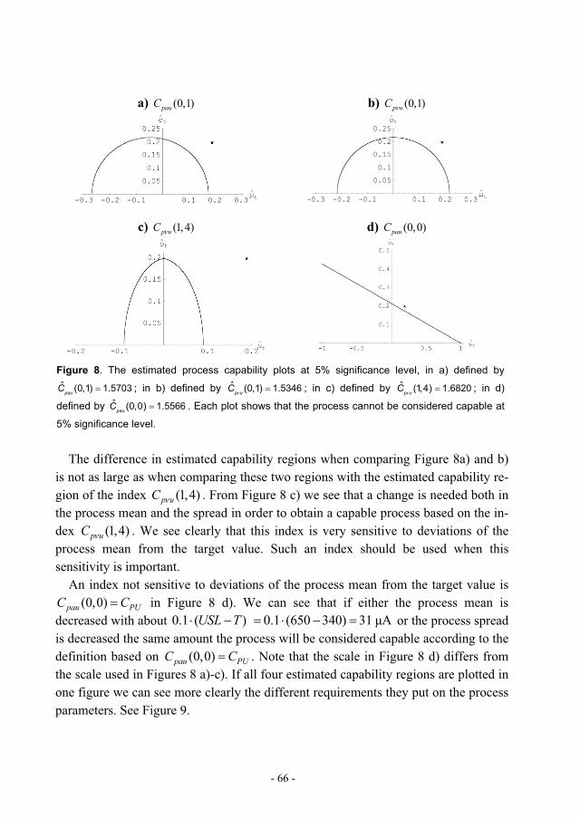
Process Capability Analysis with Focus on Indices for One-sided Specification Limits
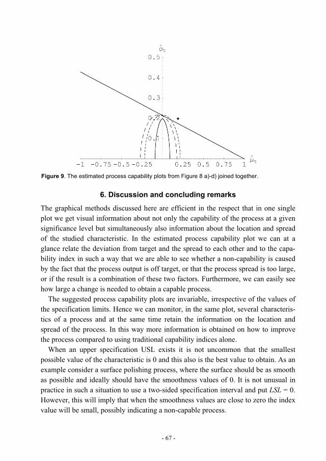
Malin Albing
Department of Mathematics Luleå University of Technology
SE-971 87 Luleå, SWEDEN
November 2006
SupervisorsProfessor Kerstin Vännman
Associate Professor Bjarne Bergquist
To Daniel
AbstractIn this thesis some aspects of process capability analysis are considered. Process ca-pability analysis deals with how to assess the capability of manufacturing processes. Based on the process capability analysis one can determine how the process performs relative to its product requirements or specifications. An important part within pro-cess capability analysis is the use of process capability indices. This thesis focuses on process capability indices in the situation when the specification limits are one-sided. The thesis consists of a summary and three papers, of which one is already published in an international journal. The summary gives a background to the research area, a short overview of the three papers, and some suggestions for future research.
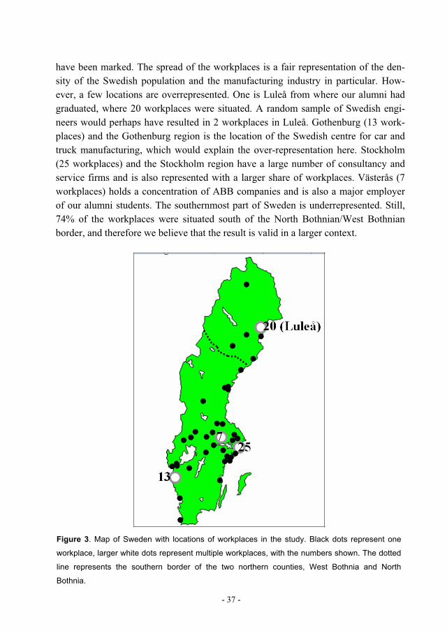
In Paper I, the frequency and use of process capability analysis together with sta-tistical process control and design of experiments, within Swedish companies hiring alumni students are investigated. We also investigate what motivates organisations to implement or not implement these statistical methods, if there are differences in use that can be related to organisational types and what will be needed to increase the use. One conclusion drawn from the results is that the students employed in the Swedish industrial sector witness a modest use of these statistical methods and use in other sectors hiring the alumni is uncommon.
In Paper II we present a graphical method useful when doing capability analysis having one-sided specification limits. This is an extension of the process capability plots previously developed for two-sided specification intervals. Under the assump-tion of normality we suggest estimated process capability plots to be used to assess process capability at a given significance level. The presented graphical approach is helpful to determine if it is the variability, the deviation from target, or both that need to be reduced to improve the capability.
In Paper III the situation with non-negative process data having a skew distribu-tion with a long tail towards large values are considered, when an upper specification limit only exists and the target value is 0. No proper indices exist for this specific situation, which is common in practice. We contribute to this area by proposing a new class of indices, ( , )MAC v , designed for skew, zero-bound distributions when an upper specification only exists and the target value is 0. This new class of indices is simple and possesses properties desirable for process capability indices. Two esti-mators of the proposed index are studied and the asymptotic distributions of these estimators are derived. Furthermore, we consider decision procedures, based on the estimated indices, suitable for deeming the process capability or not.
AcknowledgementsI have received great help and support from many persons. Without you this thesis would not have been possible to write.
First of all, I would like to thank my two supervisors Professor Kerstin Vännman and Associate Professor Bjarne Bergquist for their guidance, support and encour-agement. I would choose them as my supervisors again, any time. Kerstin, thank you for believing in me at times where I have had little confidence in myself and for the endless number of hours you spent on guiding me and explaining statistics in general and the connection to the problem at hand in particular.
I would also like to thank everyone at the Department of Mathematics at Luleå University of Technology for good companionship, especially Pär Hellström for all help with MATLAB and for inspiring me to get up to a lot of mischief. A special thanks also goes to the group of industrial statistics for all their help.
Appreciation goes to those taking part of the Female Graduate School (Forskar-skola för kvinnor), for their encouragement and for sharing valuable experiences.
The financial support from the Swedish Research Council, project number 621-2002-3823, is greatly acknowledged.
I would like to thank my family and all my friends for always being there for me and for their support and understanding during this period in my life. You are all valuable to me. A special thanks goes to Anna Andersson and Karolina Berggren for priceless moments of support and for helping me putting things in perspective.
Finally I would like to thank my husband Daniel for his never-ending love and support and for always making me smile. I am proud of being his wife.
PublicationsThe following papers are included in the thesis:
Paper I – Bergquist, B. & Albing, M. (2005). Statistical Methods – Does Anyone Really Use Them?. Total Quality Management & Business Excellence, 17, 961-972.
Paper II – Vännman, K. & Albing. M. (2005). Process Capability Plots for One-sided Specification Limits. Luleå University of Technology, Department of Mathematics, Research Report 4. SE-971 87 Luleå, Sweden. Submitted for publication.
Paper III – Albing, M. & Vännman, K. (2006). Process Capability Indices for One-sided Specification Limits and Skew Zero-bound Distributions. Luleå University of Technology, Department of Mathematics, Research Report 11. SE-971 87 Luleå, Sweden. Submitted for publication.
2. The use of process capability analysis in practice .................................................... 6
3. A background to process capability indices.............................................................. 9
4. Process capability plots for one-sided specification limits ..................................... 14
5. Process capability indices for one-sided specification limits and zero-bound skew distributions ................................................................................................................. 17
6. Concluding remarks and future research................................................................. 20
Paper I.......................................................................................................................... 27
Paper II ........................................................................................................................ 45
Paper III ....................................................................................................................... 73
1. Introduction
Process capability analysis together with statistical process control and design of ex-periments, are statistical methods that have been used for decades with purpose to reduce the variability in industrial processes and products. The need to understand and control processes is getting more and more evident due to the increasing com-plexity in technical systems in industry. Moreover, the use of statistical methods in industry is increasing by the introduction of quality management concepts such as the Six Sigma programme, where statistical methods, including process capability analysis, are important parts, see, e.g. Hahn et al. (1999).
Process capability analysis deals with how to assess the capability of a manufac-turing process, where information about the process is used to improve the capabil-ity. With process capability analysis one can determine how well the process will perform relative to product requirements or specifications. However, before assess-ing the capability of a process it is important that the process is stable and repeatable. That is, only chance causes of variation should be present. It should be noted that a process capability analysis could be preformed even if the process is unstable. How-ever, such an analysis will give an indication of the capability at that very moment only and hence, the results are of limited use.
To check if the process is stable, statistical process control is usually applied. The purpose of statistical process control is to detect and eliminate assignable causes of variation and control charts are usually used in order to determine if the process is in statistical control and reveal systematic patterns in process output. An introduction to statistical process control can be found in, e.g. Montgomery (2005a).
When the process is found stable, different techniques can be used within the con-cept of process capability analysis in order to analyse the capability, see, e.g. Mont-gomery (2005a). For instance, a histogram along with sample statistics such as aver-age and standard deviation gives some information about the process performance and the shape of the histogram gives an indication about the distribution of the studied quality characteristic. Another simple technique is to determine the shape, centre and spread of the distribution is by using a normal probability plot. However, if the underlying distribution is not normal, misleading conclusions can be drawn from the normal probability plot.
The above-mentioned tools give some approximativ information only about the process capability. The most frequently used tool when performing a capability analysis is some kind of process capability index. A process capability index is a unit less measure that quantifies the relation between the actual performance of the proc-ess and its specified requirements. In general the higher the value of the index, the lower the amount of products outside the specification limits. If the process is not
- 1 -
producing an acceptable level of conforming products, improvement efforts should be initiated. These efforts can be based on design of experiments. By using design of experiment one can for instance identify process variables that influence the studied characteristic and find directions for optimizing the process outcome. An introduc-tion to design of experiments can be found in, e.g. Montgomery (2005b).
Process capability analysis, as well as many other statistical methods, is based on fundamental assumptions. For instance, the most widely used process capability in-dices in industry today analyse the capability of a process under the assumptions that the process is stable and that the studied characteristic is normally distributed. Under these assumptions the two most frequently used indices in industry are Cp in (1) and Cpk in (2), where Cp was presented by Juran (1974) and Cpk by Kane (1986).
6pUSL LSLC (1)
and
min , 3pk
USL LSLC , (2)
where [LSL, USL] is the specification interval, is the process mean and is the process standard deviation of the in-control process. The capability index pC mea-sures the allowable range of measurements related to the actual range of measure-ments and pkC measures the distance between the expected value and the closes specification limit related to half of the actual range of measurements.
If the quality characteristic is normally distributed and the process is well centred, i.e. the process mean is located at the midpoint of the two-sided specification inter-val, implies that the number of values of the studied characteristic outside the specification limits will be small. The probability of non-conformance can be ex-pressed as
1pC
2 3 pC . In Table 1 the probability of non-conformance are stated for some given values of pC pkC. For the capability index , the probability of non-conformance will be limited by 2 3 pkC , see e.g. Pearn, Kotz & Johnson (1992).
A process is defined capable if the capability index exceeds a threshold value k,where k usually is chosen based on the probability of non-conformance given in Table 1. Mostly a process is defined capable if the index exceeds 4/3, and is if the in-dex is smaller than 4/3 but larger than 1 it is recommended to watch the process. For index values less than 1 the process is not considered capable.
- 2 -
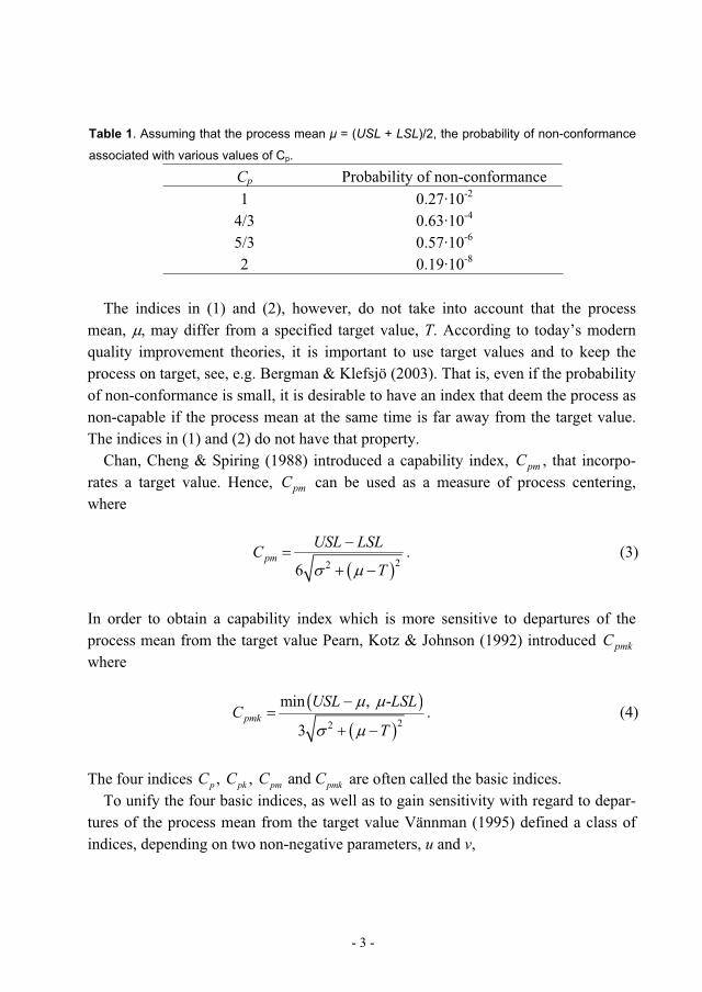
Table 1. Assuming that the process mean = (USL + LSL)/2, the probability of non-conformance
associated with various values of Cp.
Cp Probability of non-conformance 0.27·10-210.63·10-44/30.57·10-65/30.19·10-82
The indices in (1) and (2), however, do not take into account that the process mean, , may differ from a specified target value, T. According to today’s modern quality improvement theories, it is important to use target values and to keep the process on target, see, e.g. Bergman & Klefsjö (2003). That is, even if the probability of non-conformance is small, it is desirable to have an index that deem the process as non-capable if the process mean at the same time is far away from the target value. The indices in (1) and (2) do not have that property.
Chan, Cheng & Spiring (1988) introduced a capability index, , that incorpo-rates a target value. Hence, can be used as a measure of process centering, where
pmCpmC
226pm
USL LSLCT
. (3)
In order to obtain a capability index which is more sensitive to departures of the process mean from the target value Pearn, Kotz & Johnson (1992) introduced where
pmkC
22
min , -
3pmk
USL LSLC
T. (4)
, , and p pk pm pmkC C C CThe four indices are often called the basic indices. To unify the four basic indices, as well as to gain sensitivity with regard to depar-
tures of the process mean from the target value Vännman (1995) defined a class of indices, depending on two non-negative parameters, u and v,
- 3 -
22( , ) ,
3p
d u MC u v
T (5)
where d is the half length of the specification interval, i.e. d = (USL + LSL)/2, and Mis the midpoint of the specification interval, i.e. m = (USL LSL)/2. pC is obtained when (u, v) = (0, 0), pmC pmkC when (u, v) = (1, 0), when (u, v) = (0, 1), and pkCwhen (u, v) = (1, 1), respectively.
The process capability indices are theoretical quantities based on the process mean and the process variance, which in practice seldom are known. Hence, they need to be estimated from on a random sample and the estimated indices have to be treated as random variables. If the distribution of the estimated index is known it is possible to obtain decision procedures that can deem a process capable at a given significance level. Such a decision procedure usually says that the process will be considered ca-pable at significance level if the estimated index exceeds a critical value c .Alternatively a confidence interval can be derived and used for decisions about the capability. For thorough discussions of the above mention capability indices as well as others and their statistical properties see, e.g. the books by Kotz & Johnson (1993) and Kotz & Lovelace (1998) and the review paper with discussion by Kotz & John-son (2002).
Most of the published articles regarding process capability indices focus on the case when the specification interval is two-sided. Yet one-sided specifications are used in industry, see, e.g. Kane (1986) and Gunter (1989), but there have been rela-tively few articles in the statistical literature dealing with this case. Consider a situa-tion where the smallest possible value of the studied quality characteristic is zero and an upper specification limit only exists. For a situation like this it is not unusual in practice to use a two-sided specification interval and put the lower limit equal to zero. This will, however, imply that when values of the studied characteristics are close to zero the index value will be small, indicating a non-capable process, which is not correct. Besides, in this situation it is not uncommon that zero is also the best value to obtain. For instance, consider a surface polishing process, where the surface should be as smooth as possible, and ideally should have smoothness values of 0. In such a situation it is likely to find a skew distribution with a long tail towards large values rather than a normal distribution. When the studied characteristic has a skew distribution, but an index based on the normality assumption is used, the percentages of non-conforming items will be significantly different than the process capability index indicates. Hence, if we determine the capability for a process where the data are non-normally distributed, based on an index that assumes normality, we cannot
- 4 -
draw any proper conclusion about the actual process performance. See, e.g. Somer-ville & Montgomery (1996), Sakar & Pal (1997) and Chou et al. (1998).
Some process capability indices for one-sided specifications have been considered in the literature. These indices will be discussed further in Section 3. However, most of the indices for one-sided specifications assume that the studied quality character-istic is normally distributed. When it comes to analysing the capability of quality characteristics having a skew, zero-bound distribution and a target value 0 there is a lack of well functioning tools. So far we have not found any index for which a confi-dence interval or decision procedure is developed that covers this situation.
An existing problem in industry is that practitioners interpret estimated process capability indices as true values, see Deleryd (1998). To help to overcome this prob-lem Deleryd & Vännman (1999) and Vännman (2001, 2004) suggest the use of plots based on process capability indices, so called process capability plots. A process ca-pability plot is a contour plot of the capability index in the plane defined by the pro-cess parameters. The corresponding estimated process capability plots could be used to assess process capability at a given significance level. Deleryd & Vännman (1999) believe that with estimated process capability plots the uncertainty with estimated in-dices will be clearer, compared to estimated indices alone. Another advantage with using process capability plots, compared to using the capability index alone, is that one will instantly have visual information, simultaneously about the location and spread of the studied characteristics, as well as information about the capability of the process. When the process is non-capable, these plots are helpful when trying to understand if it is the variability, the deviation from target, or both that need to be re-duced to improve the capability, as well as how large a change is needed to obtain a capable process.
Deleryd (1998) identified a gap between how process capability analysis should be preformed in theory compared to how it is actually preformed in practice, and stated that process capability analysis is often misused in practice. Furthermore, from Kotz & Johnson (2002) it is clear that there is a lack of well functioning capability tools in the cases when the output is non-normally distributed. Several references in these areas are given, but more research is needed to obtain tools that can be applied by practitioners. However, process capability analysis can be a useful method for im-proving the level of performance in industrial processes, that is, if it is used in a sta-tistically sound way. Therefore we believe that is of importance to develop the theory of process capability indices in order to cover practical situations where the today most widely used indices are insufficient.
This thesis focuses on process capability indices having one-sided specification limits. As mentioned above, this is a situation common in practice but not well de-
- 5 -
veloped theoretically. The overall aim of the work presented here is to develop sim-ple and easily understood decision procedures for measuring the process capability when the specification interval is one-sided. The two last appended papers are results of accomplishing this aim. In Paper II we present a graphical approach for analysing the capability when the specification interval is one-sided and the process outcome is normally distributed. Paper II is summarised in Section 4. In Paper III we propose a new class of process capability indices to be used when the studied characteristic has a skew, zero-bound distribution and a target value at zero. A decision procedure based on this class of indices is also derived. Paper III is summarised in Section 5.
To give a more solid background to Sections 4 and 5 a Section 3 is added. In this section the cases when there is a one-sided specification interval together with both normally or non-normally distributed quality characteristic are discussed in more detail as well as the case when the process output is non-normal and the specifica-tions are two-sided.
Process capability analysis, as well as other statistical methods, has roles to play in different parts of organisational development, but the best of methods are of no value if no one uses them. Thus, an additional aim of this thesis is to seek answers to what motivates organisations to implement or not implement statistical methods, to what extent statistical methods are used within the organisations and what will be needed to increase the use. The first appended paper is a result of accomplishing this aim. In Paper I we investigate the frequency and use of statistical methods within several Swedish companies. Paper I is summarised in the next section.
2. The use of process capability analysis in practice
Deleryd (1996) preformed an extensive survey that investigates how process capa-bility analysis is accomplished within Swedish industry. The results show among other things that many organisations sometimes find the theory behind capability analysis difficult. Furthermore, it seems that many organisations are not aware of the theoretical aspects of process capability analysis or simply ignore them. However, 97 of 205 respondents claimed to work with capability analysis.
Graduate students with education in relevant statistical methods could narrow the gap, identified by Deleryd (1998), since they are familiar with the theoretical aspects behind, e.g. capability analysis. Therefore it is of interest to seek answers to how the alumni students describe the application of statistical methods within the organisations where they work. Do they come in contact with statistical methods at all? In Paper I the visibility of use of statistical process control, capability analysis and design of experiment, respectively, are investigated among a number of Swedish organisations where alumni students are working or have worked. Unreachable
- 6 -
alumni and alumni without working experience were excluded, giving a sample size of 94 respondents. 68 of the 94 respondents gave their opinion of how these statistical methods were used in a total of 98 Swedish workplaces. In 86 of those workplaces, the respondents stated that they had enough insight to judge the use of the statistical methods. The results in Paper I are based on these 86 respondents.
The results in Paper I show that respondents working in the manufacturing indus-try thought that lack of knowledge was one of the main obstacles to expanding the use of the statistical methods. Many also stated that their processes were more diffi-cult compared to examples studied at university. Furthermore, the survey does not show much evidence that the statistical methods are used in the service sector. In fact, many of the responding alumni working in the service sector believe that statis-tical methods do not fit the operations in their workplaces.
In the latest years the interest and implementation of Six Sigma have increased due to the numerous numbers of reports of its success in terms of saved costs and in-creased profits, see, e.g., Harry (1994) and Hahn et al. (1999). Other quality man-agement systems such as QS 9000 have also focused on capability analysis to a lar-ger extent. In a recent study by Gremyr et al. (2003), product development managers or quality managers from 105 manufacturing companies were telephone interviewed regarding the use of statistical methods in Swedish industry. A majority (53%) of managers stated that their companies used design of experiment and more than 60% that their companies used statistical process control and process capability analysis, respectively.
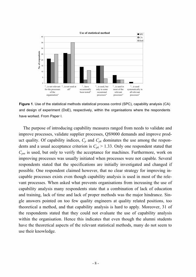
The studies preformed by Deleryd (1996) and Gremyr et al. (2003) witness about a quite common use of statistical methods in Swedish industry. However, is it possible that the definition of “use” affects the number of respondents claming that they use a certain method? Are occasional tests of a statistical method enough for respondents to say that the actual statistical method is used? Are the definitions used in different investigations similar? In Paper I the “use” of a certain statistical method is divided into several different categories in order to separate for example those organisations where “the statistical method have occasionally been tested” from those where the actual method is “used systematically in all relevant processes”. The results are shown in Figure 1 and although many organisations have tried to use statistical methods, regular use of these methods to improve processes appears to be infrequent.
- 7 -
Use of statistical method
0
5
10
15
20
25
30
35
40
"...is not relevantfor the processes
of theorganisation"
"...is not used atall"
"...haveoccasionallybeen tested"
"...is used, butonly in someoccasionalprocesses"
"...is used inmost of the
relevantprocesses"
"...is usedsystematically in
all relevantprocesses"
No.
of r
espo
nden
ts
SPCCADoE
Figure 1. Use of the statistical methods statistical process control (SPC), capability analysis (CA)
and design of experiment (DoE), respectively, within the organisations where the respondents
have worked. From Paper I.
The purpose of introducing capability measures ranged from needs to validate and improve processes, validate supplier processes, QS9000 demands and improve prod-uct quality. Of capability indices, Cp and Cpk dominates the use among the respon-dents and a usual acceptance criterion is Cpk > 1.33. Only one respondent stated that Cpm is used, but only to verify the acceptance for machines. Furthermore, work on improving processes was usually initiated when processes were not capable. Several respondents stated that the specifications are initially investigated and changed if possible. One respondent claimed however, that no clear strategy for improving in-capable processes exists even though capability analysis is used in most of the rele-vant processes. When asked what prevents organisations from increasing the use of capability analysis many respondents state that a combination of lack of education and training, lack of time and lack of proper methods was the major hindrance. Sin-gle answers pointed on too few quality engineers at quality related positions, too theoretical a method, and that capability analysis is hard to apply. Moreover, 31 of the respondents stated that they could not evaluate the use of capability analysis within the organisation. Hence this indicates that even though the alumni students have the theoretical aspects of the relevant statistical methods, many do not seem to use their knowledge.
- 8 -
3. A background to process capability indices
In this section we give a background to i) one-sided specifications and normally dis-tributed quality characteristics, ii) two sided specifications and non-normally distrib-uted quality characteristics and iii) one-sided specifications and non-normally dis-tributed quality characteristics and previous research preformed within these three areas is discussed. Even though this thesis is focusing on one-sided specification limits it is of interest to study methods for handling non-normal process data when the specifications are two-sided, in order to investigate the possibilities to adopt any of these methods for the situation of quality characteristics having a skew, zero-bound distribution and a target value 0.
One-sided specifications and normally distributed quality characteristics
The most well-known capability indices for one-sided specifications, introduced by Kane (1986), are
and 3 3PU PL
USL LSLC C , (6)
for an upper and lower specification limit, USL and LSL, respectively. As usual, is the process mean and is the process standard deviation of the in-control process, where the quality characteristic is assumed to be normally distributed. It can be noted that the indices in (6) are used to define in (2), where pkC min( , )pk PU PLC C C and hence, the indices in (6) do not take closeness to target into account. It can be noted that a lot of the research within this area consider the indices in (6). More recently Pearn & Chen (2002), Lin & Pearn (2002) and Pearn & Shu (2003) have studied tests and confidence intervals for the indices CPU and CPL in (6) and presented extensive tables for practitioners to use when applying these methods. Furthermore, Pearn & Liao (2006) consider estimates and tests of the indices in (6) in presence of measure-ment errors.
Kane (1986) also introduced the following indices, that take closeness to target into account,
and 3 3
USL T T T LSL TCPU CPL . (7)
Furthermore, Chan, Cheng & Spiring (1988) have suggested the following generali-zation of to the case where one-sided specification limit are required,
- 9 -
* *2 2 2
and 3 ( ) 3 (
pmu pmlUSL T T LSLC C
T T 2). (8)
In order to gain sensitivity with regard to departures of the process mean from the target value, Vännman (1998) defined two different families of capability indices for one-sided specification intervals, depending on two parameters, u and v, as
2 2 2 2( , ) and ( , ) ,
3 ( ) 3 ( )
where 0 and 0,
pau palUSL u T LSL u T
C u v C u vv T v T
u v (9)
and
2 2 2 2( , ) and ( , ) ,
3 ( ) 3 (
where 0 and 0, but ( , ) (0,0).
p u p lUSL T u T T LSL u T
C u v C u vv T v T
u v u v
) (10)
By changing the values of u and v we get indices with different sensitivity with re-gard to departures of the process mean from the target value. Furthermore, the in-dices in (9) and (10) generalize the indices in (6) – (8). The indices in (6) are ob-tained by setting u = 0 and v = 0 in (9). By setting u = 1, v = 0 in (10) we get the in-dices in (7) and with u = 0, v = 1 in (9) we get the indices in (7).
The estimated indices corresponding to (9) and (10) are obtained by estimating the mean by the sample mean and the variance 2 by its maximum likelihood estima-tor, i.e.
2
1 1
1 1ˆ ˆ and ( ) .n n
ii i
X X X Xn n
2i (11)
Vännman (1998) derived the distributions of the estimators of the indices in (9) and (10) under assumption that the studied quality characteristic is normally distributed and proposed tests based on the estimated indices. These results form the basis for paper II.
- 10 -
Two-sided specifications and non-normally distributed quality characteristics
Already Kane (1986) draw the attention to the problems that may occur with non-normal data and Gunter (1989), in Parts 2 and 3, highlighted this even more. To overcome these problems several approaches have been suggested. Here we discuss two common approaches, namely techniques of non-normal quantile estimation and transformations. Furthermore we consider some more recent methods for skew dis-tributions. For a thorough discussion of different methods to handle a non-normally distributed process outcome see, e.g. Kotz & Johnson (1993), Kotz & Lovelace (1998) and Kotz & Johnson (2002).
One of the first indices for data that are non-normally distributed was suggested by Clements (1989). He used the technique of non-normal quantile estimation and re-placed 6 and in Cp and Cpk with q0.99875 – q0.000135 and q0.5, respectively, where
is the th quantileq for a distribution in the Pearson family. If the distribution of the quality characteristic is normally distributed than q0.99875 – q0.000135 = 6 . Pearn & Kotz (1994) extended Clements’ method by applying it to Cpm and Cpmk. Clements’ approach does not require mathematical transformation of the data, is easy for non-statisticians to understand and no complicated distribution fitting is required, see Kotz & Lovelace (1998). However, Clements’ method requires knowledge of the skewness and kurtosis and rather large sample sizes are needed for accurate estima-tion of these quantities. Furthermore, as far as we know, the distribution for the esti-mated index has not been presented, nor tests or confidence intervals for analysing the capability of a process based on Clements’ method. Clements’ approach, with non-normal quantile estimation, has been applied to situations when the studied characteristic is assumed to follow other well-known distributions as well. For refer-ences see, e.g. Kotz & Johnson (2002).
Chen & Pearn (1997) introduced a generalization of the class of indices in (4), introduced by Vännman (1995) for normally distributed data, in purpose to handle the situation when the studied characteristic belongs to any given non-normal distribution. Their class of indices, , is based on quantiles of the underlying distribution, in the same way as Clements’ index, and defined as
( , )pC u v
( , )NpC u v
220.99865 0.00135
( , )
3 (6
Np
d u M mC u v
q q v M T
, (12)
)
q denotes the where th quantile of the cumulative distribution function F of the studied characteristic, M is the median of the distribution, T is the target value, d is
- 11 -
the half length of the specification interval, i.e. d = (USL + LSL)/2, and m is the mid-point of the specification interval, i.e. m = (USL LSL)/2. The distributions of three different estimators of this class of indices have been derived by Chen & Hsu (2003), one based on empirical quantiles, see Serfling (1980), one based on Kernel quantile estimator, see Falk (1985), and one proposed by Pearn & Chen (1997). But no test or confidence interval are derived.
Another approach when dealing with situations where the data follows some non-normal distribution is to transform the original non-normal data to normal or at least close normal. Gunter (1989) suggests data transformation in order to calculate when the process data is non-normal. Transformations of Cpk are also discussed in Rivera et al. (1995). Furthermore, Polansky et al. (1998) proposed a method for as-sessing the capability of a process using data from a truncated normal distribution, where Johnson transformations were used to transform the non-normal process data into normal.
pkC
However, one can not be sure that the capability of the transformed distribution will reflect the capability of the true distribution in a correct way, see, e.g. Gunter (1989). Furthermore, Kotz & Lovelace (1998) point out that practitioner may be un-comfortable working with transformed data due to the difficulties in translating the results of calculations back to the original scale. Another disadvantage from a practi-tioner’s point of view is that transformations do not relate clearly enough to the original specifications according to Kotz & Johnson (2002).
For the case with skew distributions and two-sided specification limits Wu et al.(1999) introduced a new process capability index based on a weighted variance method. The main idea of this method is to divide a skewed distribution into two normal distributions from its mean to create two new distributions which have the same mean but different standard deviations. Chang, Choi & Bai (2002) proposed a somewhat different method of constructing simple process capability indices for skewed populations, based on a weighted standard deviation method. Some proper-ties for the proposed indices are also investigated by Wu et al. (1999) and Chang, Choi & Bai (2002) and the estimators are compared to other methods for non-normal data. However, as far as we know the distribution for the estimated indices have not been presented, nor tests or confidence intervals for analysing the capability of a process based on the proposed indices.
Several authors have made comparative studies between different methods to han-dle non-normal process data. Van der Heuvel & Ion (2003) compared indices for skew distributions proposed by Munchechika (1986) and Bai & Choi (1997), see Van der Heuvel & Ion (2003), corresponding to Cpk, for a number of distributions. One conclusion from their study is that they believe that the true value of Cpk is in be-
- 12 -
tween the values of the indices by Munchechika and Bai & Choi for many practical situations, and together with an estimate of the maximum number of non-confor-mance, a worse-case scenario will be given. By Monte Carlo simulations Wu et al.(2001) compared , and for Clements’ method (Clements 1989), the Johnson-Kotz-Pearn method (Johnson, Kotz & Pearn 1994) and the weighted vari-ance method (Wu et al. 1999) for the Johnson family of distributions. They found that for skewed bounded cases none of these three methods performs well with re-gard of estimating the nominal value. Furthermore, Clements’ method was mislead-ing for skewed unbounded cases. For log-normal cases, the weighted variance method underestimated the nominal values while the Johnson-Kotz-Pearn method consistently overestimated the nominal values. Clements’ method did neither over-estimate nor underestimate the results on a consistent basis.
pkC pmC pmkC
One-sided specifications and a non-normally distributed quality characteristic
Process capability indices for one-sided specification and a non-normally distributed characteristic have not been discussed very much in the literature, especially not for situations with target value. Although this not an uncommon situation in industry. However, it should be noted that Clements (1989) treated the indices for one-sided specification limits corresponding to pkC , as well, i.e. CPU and CPL in (6) and Sakar & Pal (1997) considered an extreme value distribution for the CPU-case. Furthermore, Tang & Than (1999) studied estimators of in (6) for a number of methods for handling non-normal process data when the underlying distribution is Weibull and lognormal, respectively. This was done by Monte Carlo simulations. They found that methods involving transformations provide estimates of
PUC
PUC that is closer to the nominal value compared to non-transformation methods, e.g. the weighted variance method discussed by Choi & Bai (1996), see Tang & Than (1999). However, even though a method performs well for a particular distribution that method can give er-roneous results for another distribution with different tail behaviour. The effect of the tail area can be quite dramatic.
Ding (2004) introduced a process capability index based on the effective range by using the first four moments of non-normal process data. He also considered the situation with unimodal positively skewed data and proposes an index for those situations. However, the proposed index contains no target value and furthermore, as far as we know no decision procedures or tests have been presented.
It can also be mentioned that Kotz & Lovelace (1998) refer to an unpublished manuscript by Lovelace et al. (1997), where a modification of pkC for non-normal, zero-bound process data based on the lognormal quality control techniques has been
- 13 -
introduced. Nothing is mentioned about a target value or confidence intervals or tests for that modification.
In this thesis we consider the case when the specification interval is one-sided and a target value exists. Under assumption that the studied characteristic is normally distributed, the class of indices in (9) and (10) can be used for analysing the process capability since the distributions of the corresponding estimators have been derived and tests proposed by Vännman (1998). However, when the specification interval is one-sided with an upper specification USL and a specified target value equal to 0 exists it is likely that the quality characteristic has a skew, zero-bound distribution with a long tail towards large values. There is a gap in the theoretical development of capability indices for this situation and paper III in this thesis try to fill in that gap.
4. Process capability plots for one-sided specification limits
In paper II it is assumed that the studied quality characteristic is normally distributed. Based on the indices in (9) and (10) a graphical method for analysing process capa-bility when the specifications are one-sided has been derived. This method is an ex-tension of the process capability plot for two-sided specifications proposed by Deleryd & Vännman (1999) and Vännman (2001, 2004).
A process is defined to be capable if the process capability index exceeds a certain threshold value k, where . This definition can be visualized by process capabil-ity plots. These plots are based on contour curves of the indices. If we consider the case with an upper specification limit USL and let denote either of two in-dices in (9) and (10) the process capability plot is obtained by plotting
1k
( , )puC u v( , )puC u v k
as a function of the process parameters. Or, as we suggest, as functions of simple transformations of μ and , t and t, respectively, where
and t tT
USL T USL T. (13)
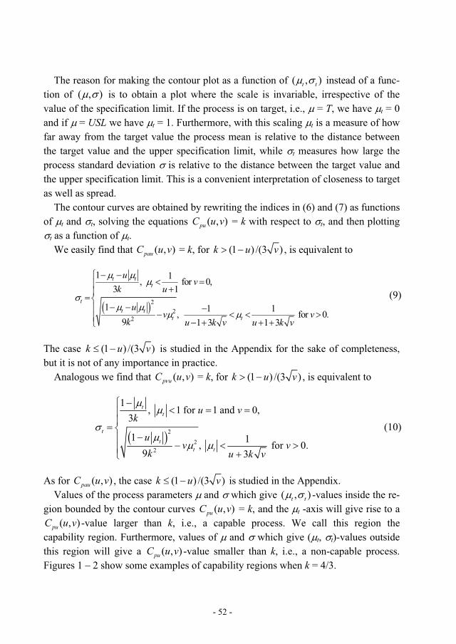
( , )t tThe reason for making the contour plot as a function of instead of a function of ( , ) is to obtain a plot where the scale is invariable, irrespective of the value of the specification limit. We easily find that = k, for ( , )pauC u v (1 ) /(3 )k u v , is equivalent to
22
2
1 1, for 0,3 1
1 1 1, for 0.9 1 3 1 3
t tt
tt t
t t
uv
k u
uv v
k u k v u k v
(14)
- 14 -
Analogously we find that = k, for ( , )p uC u v (1 ) /(3 )k u v , is equivalent to
2
22
1, 1 for 1 and 0,
3
1 1, fo 0.9 3
tt
t
tt t
u vk
uv v
k u k v
(15)
r
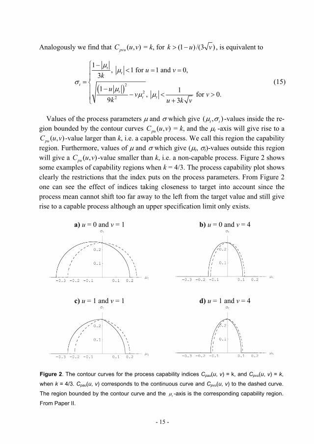
Values of the process parameters and which give ( , )t t -values inside the re-gion bounded by the contour curves = k, and the t -axis will give rise to a
-value larger than k, i.e. a capable process. We call this region the capability region. Furthermore, values of and which give ( t, t)-values outside this region will give a -value smaller than k, i.e. a non-capable process. Figure 2 shows some examples of capability regions when k = 4/3. The process capability plot shows clearly the restrictions that the index puts on the process parameters. From Figure 2 one can see the effect of indices taking closeness to target into account since the process mean cannot shift too far away to the left from the target value and still give rise to a capable process although an upper specification limit only exists.
( , )puC u v( , )puC u v
( , )puC u v
a) u = 0 and v = 1 b) u = 0 and v = 4
c) u = 1 and v = 1 d) u = 1 and v = 4
Figure 2. The contour curves for the process capability indices Cpau(u, v) = k, and Cp u(u, v) = k,
when k = 4/3. Cpau(u, v) corresponds to the continuous curve and Cp u(u, v) to the dashed curve.
The region bounded by the contour curve and the t -axis is the corresponding capability region.
From Paper II.
- 15 -
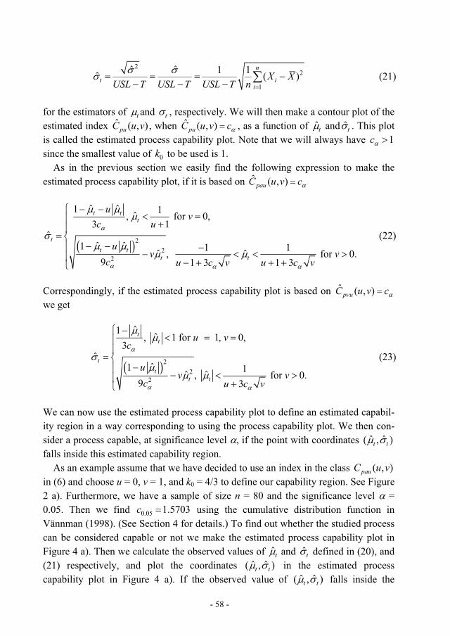
In practice the process parameters are unknown and need to be estimated. The de-cision rule will then be based on the estimated index and the process will be deemed capable if the estimated index exceeds a critical value c c, where the constant is determined so that the significance level is . In analogy with the process capability plot, we can obtain an estimated process capability plot by replacing t and t withthe corresponding maximum likelihood estimators ˆt and ˆt , respectively, and furthermore, replace k by c . We then consider a process capable, at significance level , if the point with coordinates ˆ ˆ( , )t t falls inside the estimated capability region.
As an example assume that we want to define a process capable or not based on an index in the class in (9) and choose u = 0, v = 1, and k = 4/3 to define our capability region. See Figure 2 a). Furthermore, assume that we have a sample of size n = 80 and that the significance level = 0.05. We will then find the critical value
using the cumulative distribution function in Vännman (1998). To find out whether the studied process can be considered capable or not we calculate the observed values of
( , )pauC u v
0.05 1.5703c
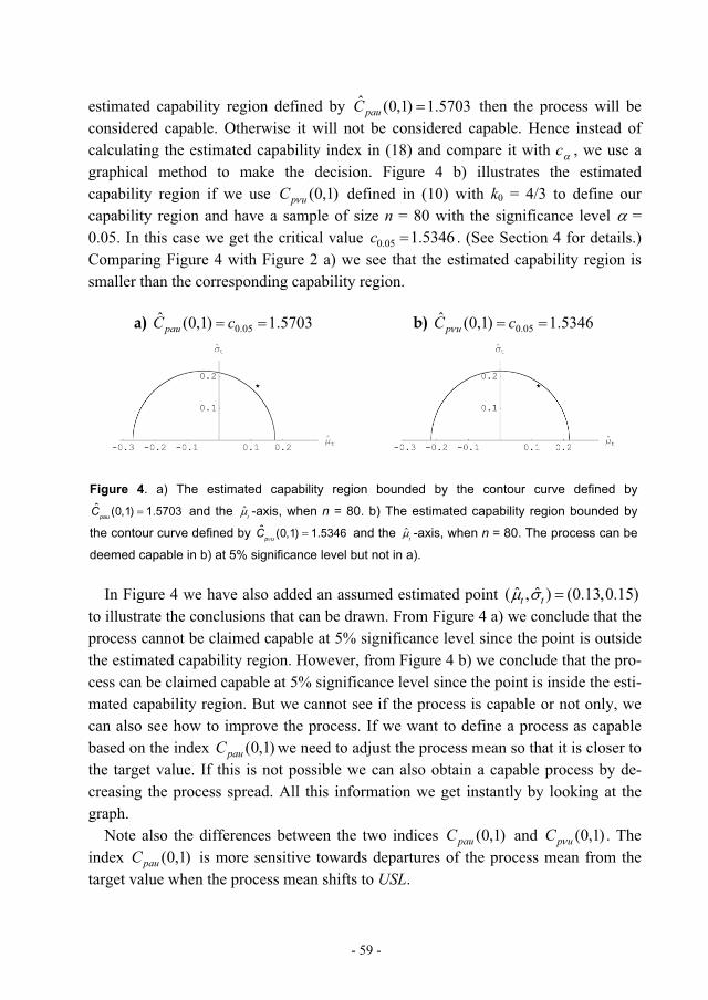
ˆt and ˆt ˆ ˆ( , )t t, and plot the coordinates in the estimated pro-cess capability plot, see Figure 3, where the estimated point ˆ ˆ( , ) (0.13,0.15)t t is added to illustrate the conclusions that can be drawn. If the observed value of
ˆ ˆ( , )t t falls inside the estimated capability region defined by then the process will be considered capable. Hence, instead of calculating the esti-mated capability index and compare it with c , we use a graphical method to make the decision. From Figure 3 we conclude that the process cannot be claimed capable at 5% significance level since the point is outside the estimated capability region. Note that the estimated capability region will always be smaller than the theoretical capability region, compare, e.g. Figure 3 with Figure 2 a). How much smaller de-pends on the sample size. The smaller the sample size the larger the difference.
ˆ (0,1) 1.5703pauC
Figure 3. The estimated capability region bounded by the contour curve defined by
and the ˆ (0,1) 1.5703pauC ˆt -axis, when n = 80. The process cannot be deemed capable at 5%
significance.
- 16 -
From a process capability plot we cannot only see if the process can be deemed capable or not, we can also see how to improve the process. If we want to define a process as capable based on the index we need to adjust the process mean so that it is closer to the target value, see Figure 3. If this is not possible we can also obtain a capable process by decreasing the process spread. All this information we get instantly by looking at the graph.
(0,1)pauC
5. Process capability indices for one-sided specification limits and zero-bound skew distributions
Assume that the studied quality characteristic has a zero-bound distribution and a target value T = 0. In general it is not realistic to assume a normal distributed quality characteristic in such a situation. The graphical approach proposed in Paper II will not be suitable for skew distributions since the distributions for the estimated indices, corresponding to (9) and (10) depends on the assumption that the underlying distri-bution is normal. A natural question it then to ask; “Is it possible to solve this prob-lem with a simple transformation”? The following illustration will give some an-swers to this question. We will here exemplify some drawbacks with using transfor-mations by using a positive skew distribution that is likely to appear in practice, namely the lognormal distribution.
Consider in (9). Let the studied characteristic X be lognormally distrib-uted with mean and variance and let the process be considered to be in statistical control. Furthermore, assume that the process mean always will be less than the upper specification limit USL and that the target value T = 0. In order to analyse the capability of the process based on we define
( , )pauC u v
( , )pauC u v lnY X . Then Y will be nor-mally distributed. However, the target value in the transformed scale will not be de-fined and hence, cannot be used. This problem could be overcome by add-ing a constant. Thus, define
( , )pauC u vln 1Z X . However, the distribution for Z is no
longer a normal distribution and hence, adding a constant is not a useful method here. Based on the discussion above it may be difficult to find a simple way of trans-forming the process data when having a target value 0. Instead a new class of indices is introduced in Paper III.
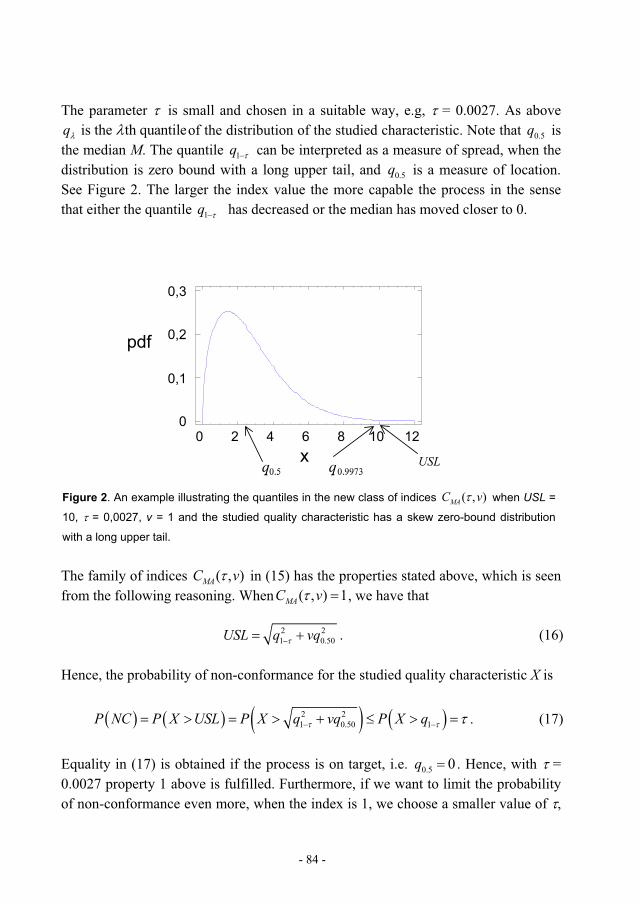
( , )MAC vThe proposed new class of indices, , depending on the two parameters and v, suitable for skew zero-bound distributions where the specifications are one-sided and a target value 0 is
2 21 0
( , ) ,MAUSLC v
q vq (16)
.5
- 17 -
where q denotes the th quantile of the cumulative distribution function F of the studied characteristic and the parameter v > 0. The parameter is small and chosen in a suitable way, e.g. = 0.0027. It is shown that the probability of non-confor-mance will be at most . A process is defined capable if ( , ) 1MAC v .
The proposed class of indices is simple and possesses properties desirable for process capability indices. For instance, for a given value of the index greater than or equal to 1 the probability of non-conformance will be small. Furthermore, the index is sensitive with regard to departures of the median from the target value, do not al-low large deviations from target even if the variance is very small and punish large departure from the target more than small.
We consider the following intuitive estimator of the th quantile q , for 0 1
ˆˆ inf : ( )q x F x , (17)
i.e. q denotes the th quantile of the empirical cumulative distribution function .As an estimator of
F( , )MAC v we then get
2 21 0.
ˆ ( , )ˆ ˆ
MAUSLC v
q vq 50
. (18)
The distribution for this estimated class of indices is derived asymptotically and pre-sented in Theorem 1. In Theorem 1 the notation AN means that the studied quantity is asymptotically normally distributed.
Theorem 1: Suppose that F possesses a positive continuous density f in the neighbourhoods of the quantiles and 0.50q 1q .
Then
21ˆ ( , ) is ( , ),MA MA CC v AN C vn
, (19)
where
2 2 22 0.50 0.50 1 1
2 22 20.50 0.50 1 11 0.50
( , ) (1 ) .4
MAC
C v v q v q q qf q f q f q f qq vq
2
2 (20)
- 18 -
In Paper III an estimator proposed by Pearn & Chen (1997) are consider as well and the asymptotic distribution of that estimator is the same as the asymptotic distribu-tion of ˆ ( , )MAC v .
Based on the result in Theorem 1 a decision rule for measuring the capability based on the estimators of ( , )MAC v is proposed, where we consider a hypothesis test with the null hypothesis 0 : ( , )MAH C v 1 and the alternative hypothesis
1 : ( , )MAH C v 1. Using the asymptotic distribution we find the critical value c by calculating the probability that ˆ ( , )MAC v c , given that , and deter-mine c
( , ) 1MAC v so that this probability is . Since the variance in the asymptotic distribution
of the estimators will depend on the underlying distribution we exemplify the rea-soning by assuming that the studied characteristic is distributed according to a Weibull distribution. The Weibull distribution is zero-bound and contains a wide range of shapes, from very skew to more or less symmetric.
Let be a random sample from the Weibull distribution measuring the studied characteristic X. The variance in the asymptotic distribution can then be ex-press as, given that ,
1 2, ,..., nX X X
( , ) 1MAC v
2 1 4 24 2 2 12 21 2 2
1 (ln 2 2 ln 2 ln 1 ln 1( )
b bb bv vb d b
1 ) , (21)
where
2 2( ) ln 1 ln 2 .b bd b v (22)
We see from (21) that the variance for the distribution of the estimated index still is not completely known, but depends on the parameter b. This implies that under the null hypothesis ˆ ( , ) ( , ) 1MA MAP C v c C v0 : ( , )MAH C v 1 the probability will vary depending on the value of b.
In practice the values of the shape parameter b is seldom known. To form a deci-sion rule we suggest an estimate of b to be used. Two different estimators of b are considered, the maximum likelihood estimate of b and the lower confidence limit of a 100(1- )% two-sided confidence interval of b. The lower limit is used because the variance 2
1 decreases in b. Thus a process, where the studied characteristic is Weibull distributed, is considered capable if
21
1ˆ ˆ( , ) 1 ,MAC vn
(23)
- 19 -
21ˆ denotes an estimate of 2
1where in (21) based on one of the two estimators of b.Note that these results are valid for the estimator proposed by Pearn & Chen (1997) as well.
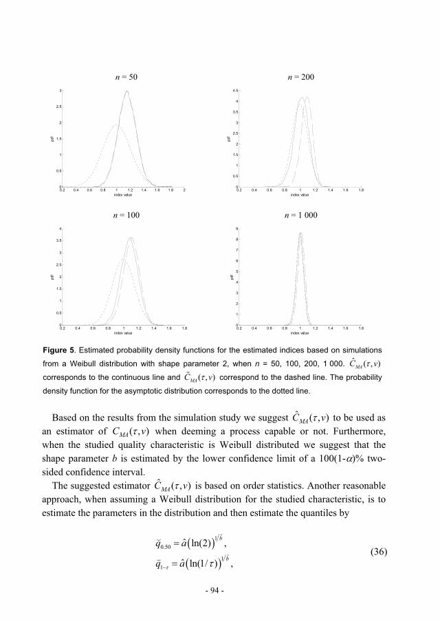
Under assumption that the studied characteristic is Weibull distributed, a simula-tion study is preformed in order to investigate how good the approximation of the significance level of the test is when the sample size n is finite and to compare the two different ways to estimate 2
1 in (21). Based on the results from the simulation study we suggest the estimator based on empirical quantiles to be used when deem-ing a process capable or not. Furthermore, when the studied quality characteristic is Weibull distributed we suggest that the shape parameter b is estimated by the lower confidence limit of a 100(1- )% two-sided confidence interval.
Even though the proposed decision rule is based on the asymptotic distribution for the estimator, the simulation study shows that the decision procedure works well for as small sample sizes as 50 when shape parameter , i.e. when the underlying distribution is not too skew. That is, when the estimator based on the empirical quantiles is used and the shape parameter b in the Weibull distribution is estimated by the lower confidence limit of a 100(1- )% two-sided confidence interval. It also works well for b = 1.5 if the sample size is at least 100. The more skew the distribu-tion is the larger sample size is needed.
2b
6. Concluding remarks and future research
In this thesis some aspects of process capability analysis have been considered. This section concludes the thesis and gives some suggestions for future research.
Concluding remarks
One of the aims with writing this thesis has been to seek answers to what motivates organisations to implement or not implement statistical methods, to what extent sta-tistical methods are used within the organisations and what will be needed to increase the use. The results in Paper I show that even though many of the respondent organi-sations have tried to use capability analysis, few of them use it systematically in most of the relevant processes. Compared to the results form other surveys in Swedish in-dustry, see Deleryd (1996) and Gremyr et al. (2003), the survey preformed in Paper I indicates that the use of capability analysis is less common, even if use is defined as “capability analysis has at least occasional been tested”. These results are a contribu-tion to the discussion regarding capability analysis and show that proper tools are not needed only, but also good implementation strategies. The results in Paper I are also important from an educating point of view since they show that universities need to
- 20 -
focus on the practical aspect of statistical methods to a larger extent. Furthermore, many of the respondents with proper method training do not seem to come in contact with statistical methods at their workplaces.
The other aim of this thesis has been to develop simple and easily understood de-cision procedures for measuring the process capability when the specification inter-val is one-sided. The case when the studied quality characteristic can be assumed normally distributed has been considered, as well as the case when the characteristic is skewly distributed.
In the estimated process capability plot for one-sided specifications, proposed in Paper II, we could at a glance relate the deviation from target and the spread to each other and to the capability index. Hence, we are able to see whether a non-capability is caused by the fact that the process output is off target, or that the process spread is too large, or if the result is a combination of these two factors. Furthermore, we can easily see how large a change is needed to obtain a capable process.
The capability indices were introduced to focus on the process variability and closeness to target and relate these quantities to the specification interval and the tar-get value. We believe that the plots discussed in Paper II will do this in a more effi-cient way than the capability index alone. It is also well known that the visual impact of a plot is more efficient than numbers, such as estimates or confidence limits. Fur-thermore, with today’s modern software the plots proposed here are easy to generate.
Several different methods for handling non-normal process data have been pro-posed and discussed in literature. However, there is a gap in the theoretical develop-ment of capability indices for situations when there is an upper specification USL and a pre-specified target value equal to 0 and the quality characteristic of interest has a skew, zero-bound distribution with a long tail towards large values. Paper III con-tributes to this area by proposing a new class of indices which covers the situation described above. This class of indices, ( , )MAC v , is simple and possesses properties desirable for process capability indices. Furthermore, decision procedures based on the estimated indices suitable for measuring the process capability are derived.
Suggestions for future research
By experience, it is difficult to receive acceptance for new indices in industry. However, our proposed index is simple and a decision procedure is presented as well. Furthermore, we believe that an extension of the graphical approach proposed in Pa-per II to the case of zero-bound skew distributions would facilitate the understanding and use of the proposed class of indices ( , )MAC v . Hence, this would be of interest to develop.
- 21 -
The decision rule proposed in Paper III is based on the asymptotic distribution of the estimators. The simulation study shows that when the underlying distribution is a Weibull distribution and not too skew, the proposed decision rule works well for small sample sizes if the estimator is based on empirical quantiles and the shape pa-rameter b is estimated by the lower confidence limit of a 100(1- )% two-sided con-fidence interval. However, in order to obtain a decision rule with known significance level when the distribution is highly skewed and the sample size is small or moderate the exact distribution for the estimator is needed.
( , )MAC vThe suggested estimator of is based on order statistics. Another reason-able approach, when assuming a Weibull distribution for the studied characteristic, is to base the estimator of ( , )MAC v on maximum likelihood estimators of the parame-ters in the distribution. From the simulation it is clear that the variance for this esti-mator will be smaller than the variance for the estimator based on order statistics. However, in order to be able to base a decision rule on this estimator its exact or asymptotic distribution needs to be derived. Furthermore, it is of interest to investi-gate other distribution than the Weibull distribution.
The results regarding the asymptotic distributions are based on the assumption that the underlying distribution is continuous. An interesting case to consider in the future is when the quality characteristic of interest may attain zero values. A possible distri-bution for such a quality characteristic is a non-standard mixture of distributions. Then we assume that the studied characteristic X is zero with probability p and posi-tive with probability 1 – p. This can be expressed as
0 with probability , with probability 1 ,
pX
Z p (24)
where Z is a positive continuous random variable with a skew distribution. With a non-standard mixture of distributions, where p 0.5, it is also possible to obtain the process on target, when T = 0.
As mentioned before there is a gap in the theoretical development of capability in-dices for situations when there is an upper specification and the target value is equal to 0 and the quality characteristic of interest has a skew, zero-bound distribution with a long tail towards large values. With the results in Paper III we have started to fill in this gap and we believe that it is of importance to continue investigating the case, which is also a practical case of interest.
- 22 -
7. References
Bai, D. S. & Choi, I. S. (1997). Process Capability Indices for Skew Populations. Manuscript, Korea Advanced Institute of Science and Technology, Teajon, Korea.
Bergman, B. & Klefsjö, B. (2003). Quality from Customer Needs to Customer Sat-isfaction. Second edition. Studentlitteratur, Lund.
Chan, L. K., Cheng, S. W. & Spiring, F. A. (1988). A New Measure of Process Ca-pability: pmC . Journal of Quality Technology, 20, 162-175.
Chang, Y. S., Choi, I. S. & Bai, D. S. (2002). Process Capability Indices for Skewed Populations. Quality and Reliability Engineering International, 17, 397-406.
Chen, K. S. & Pearn, W. L. (1997). An Application of Non-normal Process Capabil-ity Indices. Quality and Reliability Engineering International, v 13, 355-60.
Chen, S.-M. & Hsu, Y.-S. (2003). Asymptotic Analysis of Estimators for Based on Quantile Estimators. Nonparametric Statistics, v 15, 137-150.
( , )NpC u v
Choi, I. S. & Bai, D. S. (1996). Process Capability Indices for Skewed Populations. Proceedings 20th Int. Conf. on Computer and Industrial Engineering, 1211–1214.
Chou, Y.-M., Polansky, A. M. & Mason, R. L. (1998). Transforming Non-normal Data to Normality in Statistical Process Control. Journal of Quality Technology,30, 133-141.
Clements, J. A. (1989). Process Capability Calculations for Non-normal Distribu-tions. Quality Progress, 22, 95-100.
Deleryd, M. (1996). Process Capability Studies in Theory and Practice. Licentiate thesis, Luleå University of Technology.
Deleryd, M. (1998). On the Gap Between Theory and Practice of Process Capability Studies. Journal of Quality & Reliability Management, 15, 178-191.
Deleryd, M. & Vännman, K. (1999). Process Capability Plots—A Quality Improve-ment Tool. Quality and Reliability Engineering International, 15, 1-15.
Ding, J. (2004). A Method of Estimating the Process Capability Index from the First Four Moments of Non-normal Data. Quality and Reliability Engineering Interna-tional, 20, 787-805.
Falk, M. (1985). Asymptotic Normality of the Kernel Quantile Estimator. The An-nals of Statistics, 13, 428-433.
Gremyr, I., Arvidsson, M. & Johansson, P. (2003). Robust Design Methodology: Status in Swedish Manufacturing Industry, Quality and Reliability Engineering International, 19, 285-293.
Gunter, B. H. (1989). The Use and Abuse of : Parts 1-4. Quality Progress, 22, January, 72-73; March, 108-109; May, 79-80; July, 86-87.
pkC
- 23 -
Hahn, G. J., Hill, W. J., Hoerl, R. W. & Zinkgraf, S. A. (1999). The Impact of Six Sigma Improvement—A Glimpse into the Future of Statistics. The American Statistician, 53, 208-215.
Harry, M. J. (1994). The Vision of Six Sigma: A Roadmap for Breakthrough. Phoe-nix, AZ, Sigma Publishing Company.
Johnson, N. L., Kotz, S. & Pearn, W. L. (1994). Flexible Process Capability Indices. Pakistan Journal of Statistics, 10, 23-31.
Juran, J. M. (1974). Jurans Quality Control Handbook. Third edition. McGraw Hill, New York.
Kane, V. E. (1986). Process Capability Indices. Journal of Quality Technology, 18, 41-52.
Kotz, S. & Johnson, N. L. (1993). Process Capability Indices. Chapman & Hall, London.
Kotz, S. & Johnson, N. L. (2002). Process Capability Indices—A Review, 1992 – 2000 with Discussion. Journal of Quality Technology, 34, 2-53.
Kotz, S. & Lovelace, C. R. (1998). Introduction to Process Capability Indices: The-ory and Practice. Arnold, London.
Lin, P. C. & Pearn, W. L. (2002). Testing Process Capability for One-sided Specifi-cation Limit with Application to the Voltage Level Translator. MicroelectronicsReliability, 42, 1975-1983.
Lovelace, C. R., Swain, J. & Messimer, S. (1997). A Modification of for Non-normal, Zero-bound Process Data Using Lognormal Quality Control Techniques. Manuscript, University of Alabama in Huntsville, Huntsville, AL, USA.
pkC
Montgomery, D. C. (2005a). Introduction to Statistical Quality Control. Fifth edi-tion. John Wiley & Sons, Hoboken, NJ.
Montgomery, D. C. (2005b). Design of Experiments. Sixth edition. John Wiley & Sons, Hoboken, NJ.
Munechika, M. (1986). Evaluation of Process Capability for Skew Distributions. Proceedings 30th EOQC Conference, Stockholm, 383-390.
Pearn, W. L. & Chen, K. S. (1997). Capability Indices for Non-normal Distributions with an Application in Electrolytic Capacitor Manufacturing. Microelectronicsand Reliability, 37, 1853-1858.
PUC PLCPearn, W. L. & Chen, K. S. (2002). One-Sided Capability Indices and :Decision Making with Sample Information. International Journal of Quality and Reliability Management, 19, 221-245.
Pearn, W. L. & Kotz, S. (1994). Application of Clements’ Method for Calculating Second- and Third-generation Process Capability Indices for Non-normal Person-ian Populations. Quality Progress, 7, 139-145.
- 24 -
Pearn, W. L., Kotz, S. & Johnson, N. L. (1992). Distributional and Inferential Prop-erties of Process Capability Indices. Journal of Quality Technology, 24, 216-231.
Pearn, W. L. & Liao, M.-Y. (2006). One-sided Process Capability Assessment in the Presence of Measurement Errors. Quality and Reliability Engineering Interna-tional, 22, 771-785.
Pearn, W. L. & Shu, M.-H. (2003). An Algorithm for Calculating the Lower Confi-dence Bounds of PUC PLC and with Application to Low-drop-out Linear Regula-tors. Microelectronics Reliability, 43, 495-502.
Polansky, A. M., Chou, Y. M. & Mason, R. L. (1998). An Algorithm for Fitting Johnson Transformations to Non-normal Data. Journal of Quality Technology, 31, 345-350.
Rivera, L. A. R., Hubele, N. F. & Lawrence, F. P. (1995). Cpk Index Estimating Using Data Transformation. Computers & Industrial Engineering, 29, 55-58.
Sarkar, A. & Pal, S. (1997). Estimation of Process Capability Index for Concentric-ity. Quality Engineering, 9, 665-671.
Somerville, S. E. & Montgomery, D. C. (1996). Process Capability Indices and Non-normal Distributions. Quality Engineering, 9, 305-316.
Serfling, R. J. (1980). Approximation Theorems of Mathematical Statistics. John Wiley and Sons, New York.
Tang, L. C. & Than, S. E. (1999). Computing Process Capability Indices for Non-normal Data: A Review and Comparative Study. Quality and Reliability Engi-neering International, 15, 339-353.
Van den Heuvel, E. R. & Ion, R. A. (2003). Capability Indices and the Proportion of Nonconforming Items. Quality Engineering, 15, 427-439.
Vännman, K. (1995). A Unified Approach to Capability Indices. Statistica Sinica, 5, 805-820.
Vännman, K. (1998). Families of Capability Indices for One-sided Specification Limits. Statistics, 31, 43-66.
Vännman, K. (2001). A Graphical Method to Control Process Capability. Frontiersin Statistical Quality Control, No 6, Editors: Lenz, H.-J. & Wilrich, P.-TH. Physica-Verlag, Heidelberg, 290-311.
Vännman, K. (2004). Safety Regions in Process Capability Plots. Research report 2004-01, Department of Mathematics, Luleå University of Technology, SE-971 87 Luleå. Submitted for publication.
Wu, H,-H., Swain, J. J., Farrington, P. A. & Messimer, S. L.(1999). A Weighted Variance Capability Index for General Non-normal Processes. Quality and Reli-ability Engineering International, 15, 397-402.
- 25 -
Wu, H.-H. & Swain, J. J. (2001). A Monte Carlo Comparison of Capability Indices when Processes are Non-normally Distributed. Quality and Reliability Engineer-ing International, 17, 219-231.
- 26 -
PAPER I
Statistical Methods – Does anyone really use them?
Published as
Bergquist, B. & Albing, M. (2005). Statistical Methods – Does Anyone Really Use Them?. Total Quality Management & Business Excellence, 17, 961-972.
- 27 -
Statistical Methods – Does Anyone Really Use Them?
BJARNE BERGQUIST* & MALIN ALBING**
*Department of Industrial Economics & Social Sciences, Division of Quality & Environmental Management;**Department of Mathematics, Luleå University of Technology, Sweden
Abstract: Students taking courses in quality management at Luleå University of Technology receive extensive education in statistical methods. To improve the edu-cation and to understand what kind of competence students need when they graduate, a survey examining how and to what extent the methods Statistical Process Control, Capability Analysis and Design of Experiments are used by organisations hiring the alumni was preformed. The result shows that the students employed in the Swedish industrial sector witness a modest use. Use of statistical methods in other sectors hiring the alumni is uncommon. Lack of competence and resources within the or-ganisations are stated as hindrances to expanded use. Conclusions from the study are that implementation techniques must be emphasized in the curriculum and that dif-ferent types of courses should be given – practical, hands-on courses for engineers, managers and others working in organisations. Furthermore, courses offered at uni-versities must have a strong focus on practical problems such as difficulties random-izing experiments and that graphical methods should be favoured.
Keywords: Capability index, Capability indices, Experimental design, Design of experiments, Statistical Process Control Survey, Use, Sweden
- 29 -
Introduction
Statistical methods (SMs) such as Statistical Process Control (SPC), Capability Analysis (CA) and Design of Experiments (DoE) have been used for decades to im-prove the quality of processes and products in quality management, see Bergman & Klefsjö (2003). The SMs have mostly been used in manufacturing industry, but also in other types of problems such as to understand customer needs and behaviour, see Green & Srinivasan (1978) or Gustafsson et al. (1999). The use of SMs are further amplified by recent quality management trends such as Six Sigma; see Harry (1994) or Hahn et al. (1999). SMs have also found applications in service, see Mundy et al. (1990), Kumar et al. (1996) or Mason & Antony (2000), and this use is also ampli-fied by the broadened focus of Six Sigma, see Hoerl (2001).
SMs have roles to play in different parts of organisational development, but the best of methods are of no value if no one uses them. In Swedish studies of the use of SMs performed in the mid 90s, the use ranged from non-existent to moderate. In a survey by Deleryd (1996), the use of process capability measurements in Swedish industry was investigated and 97 of 205 respondents claimed to work with CA. However, an investigation of companies in the Swedish counties of North Bothnia and West Bothnia regarding the utilization of quality methods concluded that the use of DoE was around 6% and that the use of SPC and CA was less than 5% (Bäcklund et al. 1995). In a recent study by Gremyr et al. (2003), product development man-agers or quality managers from 105 manufacturing companies were telephone inter-viewed regarding the use of statistical methods in Swedish industry. A majority (53%) of managers stated that their companies used DoE and more than 60% that their companies used SPC and CA respectively. The findings by Gremyr et al. (2003)are in agreement with a British study by Thornton et al. (2000), who investigated the use of SMs in 19 companies of which all used SPC, most used CA and about one third used some form of robust design methodology, including DoE.
Studies of the use of SMs outside the industrial sector are rare. A British survey by Redman et al. (1995) concluded that 18% of service organisations, private or public alike, used SPC. Witt & Clark (1990) studied if SPC was used to improve quality in British tourism. The result was that 15 of 75 of respondents stated that use of SPC was frequent and another 9 respondents stated that use of SPC was occasional.
A problem in all the studies is of course what respondents define as “use”. Is the occasional test of an SM enough for respondents to say that it is used, and are the definitions used in different investigations similar? Comprehension of SMs is vital if respondents should evaluate their use, and answers regarding use and applicability might be misleading if respondents lack proper method comprehension. Kotz & Johnson (2002) state that the gap between practitioners and theoreticians in the field
- 30 -
of CA is wide, and that the gap has widened during the last 10 years. It appears likely that the same is true for SPC and DoE as well.
The authors of this paper are teaching quality management and applied statistical methods to Swedish engineering students. As teachers we often receive questions from students regarding how frequently the methods we teach are used. Other ques-tions from students are how likely it is that, when they have graduated, they will transform their theoretical knowledge into practice at their workplaces. These ques-tions are certainly legitimate and deserve a well-founded response. However, the re-sponses we have given to such questions have generally been a mix of belief, knowl-edge and optimism. Optimism since we want the use to be high to retain high credi-bility. Nonetheless, in contact with Swedish industry, directly or indirectly, by super-vising students, we were led to believe that use of SMs was less common than re-ported by Deleryd (1996) and Gremyr et al. (2003).
The apparent differences between the stated utilization of SMs based on interviews and surveys and student feedback were unsettling. Was the difference due to the lim-ited access of our students or were they actually doing projects or diploma work in organisations that did not use statistical methods? Was use of SMs less frequent than previous studies had indicated, and if so why? Was the use of SMs in industry, ser-vice, research, or product development strong enough to be visible to new engineers entering their working life or were there only a few rare examples of this sort? To answer these questions, an investigation of the visibility of the use of these SMs in Swedish organisations was performed. Furthermore, graduate students with method training in SMs could narrow the gap between theoreticians and practitioners. Thus, a follow-up of how organisations with which they had worked use SMs was consid-ered interesting.
Purpose
The main purpose of the investigation was therefore to determine how our alumni would describe the frequency and use of SMs in their workplaces and also how the SMs are used. Secondary purposes were to seek answers to what motivated organi-sations to implement or not implement SMs, to seek differences in use related to or-ganisational types, and to find out what was needed to increase the use.
Method
The survey, executed as an inquiry, was limited to alumni students who had taken their final courses in quality management at Luleå University of Technology. The sampling frame was based on students who had taken university courses covering
- 31 -
these specific SMs with a length of at least three full-time weeks. It was therefore possible to ensure that the respondents were well aware of our views and definitions of these methods, and explanations of SMs in the questionnaire could be held short. Our hope was that the response rate should be high, as the respondents were our own alumni. However, a possible bias if results were compared to general use, for in-stance industrial or Swedish use, could be that the respondents with method training would be more prone to seek work in companies interested in these skills. Still, the target population was considered ideal to answer the question: “How likely is it that graduated students meet SMs?”.
The sampling frame was a mix between a convenience sampling and a total inves-tigation, in such a way that the total population of our alumni was included. Since one of the reasons for starting the investigation was to examine how likely it is that alumni will come into contact with SMs in their workplaces, the sampling frame was considered relevant. Using another type of sampling frame and selection method, e.g. a randomly chosen sample from a database containing Swedish companies would en-able different types of general statements, but would not enable commenting the alumni students. It was also considered more important to use a respondent group with method training on the basis of the questions we wanted answered.
A preliminary version of the questionnaire was tested on a group of researchers at Luleå University of Technology teaching questionnaire design and analysis. The three sections of the questionnaire focused on SPC, CA and DoE, respectively. Each section included questions where respondents rated the organisational use of each SM using Likert scales. The degrees of use of the SMs were divided into seven statements about each company or organisation with which they were acquainted ranging from the SM not being relevant for the processes of the workplace to the SM being used systematically in all processes. In addition, the questionnaire included open questions aiming at understanding why the SMs were used, how results are used, and what the obstacles are to increasing the frequency of use. The question-naire was designed so that respondents could rate the use of several organisations they had worked with.
Unreachable alumni and alumni without working experience were excluded, giv-ing a sample size of 94 respondents. The first round of questionnaires was sent out in November 2004 and the respondents were given three weeks to answer the question-naire, resulting in 22 responses. A reminder where each missive letter was hand-signed by the researchers and the name of the respondent was pre-written was sent in December 2004, which resulted in 40 additional responses. A second reminder was sent in January 2005, resulting in six more responses. This gives a total of 68 re-sponses and a response rate of 72%. In an effort to reduce speculative answers, only
- 32 -
responses where the respondent had seen an occasional or more frequent use were analysed in connection to questions such as why the organisation had implemented the SM.
Affinity diagrams were used to group the answers of the open questions. Open an-swers were also separated on the basis of the respondents’ answers to the closed questions, enabling comparison of open answers of respondents reporting rare or no use of SMs to open answers of respondents reporting frequent use.
Results
The 68 respondents gave their opinion of how the SMs were used in a total of 98 Swedish workplaces. In 86 of the workplaces, the respondents stated that they had enough insight to judge the use of SMs. The workplaces were classified as small or large based on the number of employees. If the number was larger than 50, the or-ganisation was considered large. The workplaces were also separated into service or industrial type organisations, see Table 1.
Quantitative results
A majority of the respondents indicated sporadic or no use of the SMs in the organisations where they had worked, and this was independent of the SM in question, see Figure 1. Of the 37 workplaces where SPC had at least been tested, only one company was said to use SPC systematically in all relevant processes and 7 companies were said to use SPC in most of the relevant processes. For CA (21 workplaces) and DoE (18 workplaces), none of the companies was reported to use the SM systematically in all relevant processes, and only at three companies were SMs said to be used in most relevant processes.
Table 1 is a two - way representation of the use of SMs, categorized by organisational type and organisational size. “Use” in Table 1 is defined as one SM has at least been tested (numbers within parenthesis is number of organisations within each category).
There is a difference between how respondents estimated the use of SMs in their organisations depending on the size of the organisation. Respondents within large or-ganisations see use of SMs more often. The use in service organisations is less fre-quent than in industrial organisations. Furthermore, there is no clear tendency for neither small nor large organisations to be either industrial or service types and thus, the effect of company size does not explain the more frequent use in larger firms compared to that in small ones and vice versa; the size effect does not explain why industrial firms are more frequent users.
- 33 -
Depending on SM, 42% (SPC), 36% (CA) and 44% (DoE) the respondents that had worked in the non-industrial sector had the opinion that use of SMs was irrelevant for the type of work performed there. For the industrial organisations, the SMs were classified as irrelevant for 10% (SPC) 8% (CA) and 14% (DoE).
Table 1. The numbers of organisations that have been classified by the respondents to use statis-
tical mecthods. Cell numbers represents use of SMs within category (number of organisations
within category in parenthesis). Small org. (< 50 employees) Large org. Total
Industry 1 (7) 31 (43) 32 (50)
Non-industrial 0 (9) 7 (27) 7 (36)
Total 1 (16) 38 (70) 39 (86)
Use of statistical method
0
5
10
15
20
25
30
35
40
"...is not relevantfor the processes
of theorganisation"
"...is not used atall"
"...haveoccasionallybeen tested"
"...is used, butonly in someoccasionalprocesses"
"...is used inmost of the
relevantprocesses"
"...is usedsystematically in
all relevantprocesses"
No.
of r
espo
nden
ts
SPCCADoE
Figure 1. Use of statistical methods in the organisations where the respondents have worked.
Qualitative results SPC
Based upon the open answers of the respondents that had seen use of the SMs (pre-dominantly large manufacturing firms), a conclusion is that the large majority of
- 34 -
companies had the motive to reduce or control variation when SPC and control charts were introduced. 12 respondents stated that SPC results were used by the company to improve processes; 5 respondents stated that the results from SPC were not used at all. When asked what prevents companies from increasing the use of SPC, 13 re-spondents thought that a combination of lack of education and training, lack of time and lack of proper SMs was the major hindrance. 3 stated that fear of change was the main obstacle. Single answers pointed to laziness, too theoretical a method, too small series, and a general statement that SPC is hard to apply.
Qualitative results CA
Compared to reasons for introducing SPC, the purpose of introducing capability measures shifted more and ranged from needs to validate and improve processes (six answers), validate supplier processes (two answers), QS9000 demands (two answers) and improve product quality (two answers). Of capability indices, Cp and Cpk domi-nated the use and a usual acceptance criterion was to have Cpk > 1.33. Three work-places used tougher acceptability criteria (Cp > 1.67) for new processes. Work on improving processes was usually initiated (eight of ten) when processes were not ca-pable. The respondents gave similar reasons for what prevented further use of CA as for what prevented further use of SPC.
Qualitative results DoE
The reasons for introducing DoE was even more varied and some excerpts were: “…need to reduce process variation”, “…too many variables for one-factor-at-a-time type experiments”, “…interested in new technology”, “…need for improving process quality”. All respondents (11) that discussed how companies had worked with DoE stated that full or reduced factorial designs were used. One company also used split-plot experiments, one used mixture experiments and one had used Taguchi type ex-periments. Albeit split-plot experiments were only used by one company, all but one respondent stated that the experimental arrangement usually was non-random and that this was due to difficulties adjusting certain factors. Lack of management com-petence as well as engineering competence was stated as the main obstacle to a more frequent use of DoE. However, one respondent stated that DoE was too resource de-manding.
Reliability and validity
Other surveys measuring the use of statistical or other quality related SMs have ob-served response rates in the 15 – 27 % range, see Witt & Clark (1990), Mathews et
- 35 -
al. (2001), Redman et al. (1995) or Deleryd (1996). Response rates of alumni sur-veys are often in the 32-36% range, see Porter & Umbach (2001). The response rate of the study (72%) is considerably higher than that of other surveys of statistical methods. The response rate was higher in the first reminder than in the first survey, which was probably due to the personal touch with hand-written names and signa-tures of the researchers. The high response rate of this survey compared to that of other studies is most likely related to the selected response group in combination with the personal touch. The first survey and first reminder included enough re-sponses to estimate if the respondents had answered differently in the reminder than in the first survey. The differences of stated use were compared for all SMs; for a SPC example see Figure 2. The profiles of the two groups of answers were consid-ered fairly equal, and this result was about the same for all SMs. We thus assume that the answers were not dependent upon whether the respondent had answered directly or more reluctantly. Led by this result, we assume that answers of non-respondents would not have led to markedly different results.
Use of SPC in organisations
0
2
4
6
8
10
12
14
"...is not relevantfor the processes ofthe organisation"
"...is not used atall"
"...haveoccasionally been
tested"
"...is used, but onlyin some occasional
processes"
"...is used in mostof the relevant
processes"
"...is usedsystematically in
all relevantprocesses"
No:
ans
wer
s
1:st survey1:st reminder
Figure 2. Use of SPC in organisations where respondents have worked in the first survey and
the first reminder survey.
Since the study by Bäcklund et al. (1995) showed little use of SMs in Sweden’s northernmost counties, North Bothnia and West Bothnia, a concern was that results might be hard to analyze, if the distribution of the location of workplaces was highly skewed toward the northern part of Sweden. In Figure 3, the workplaces in the study
- 36 -
have been marked. The spread of the workplaces is a fair representation of the den-sity of the Swedish population and the manufacturing industry in particular. How-ever, a few locations are overrepresented. One is Luleå from where our alumni had graduated, where 20 workplaces were situated. A random sample of Swedish engi-neers would perhaps have resulted in 2 workplaces in Luleå. Gothenburg (13 work-places) and the Gothenburg region is the location of the Swedish centre for car and truck manufacturing, which would explain the over-representation here. Stockholm (25 workplaces) and the Stockholm region have a large number of consultancy and service firms and is also represented with a larger share of workplaces. Västerås (7 workplaces) holds a concentration of ABB companies and is also a major employer of our alumni students. The southernmost part of Sweden is underrepresented. Still, 74% of the workplaces were situated south of the North Bothnian/West Bothnian border, and therefore we believe that the result is valid in a larger context.
Figure 3. Map of Sweden with locations of workplaces in the study. Black dots represent one
workplace, larger white dots represent multiple workplaces, with the numbers shown. The dotted
line represents the southern border of the two northern counties, West Bothnia and North
Bothnia.
- 37 -
The answers of respondents that had stated that they were working at the same work-place were also compared and the differences in answers were considered small. A conclusion is therefore that the results regarding the investigated workplaces are valid.
Discussion
The sampling frame
Compared to the regular Swedish population or to the average engineer, our alumni students have a better knowledge of the SMs. We thus expect them to be more often seen in organisations that work with these methods or feel the need for them, as their background would fit the offered job descriptions. The workplaces of alumni groups are also highly skewed towards work in the private sector and in the manufacturing industry. It is in the manufacturing industry that we see the most frequent use of SMs. A conclusion from this is that if the sample had been a random sample of Swedish organisations, the frequency of use would have been much lower. Notice that 88% of the respondents answered that they could evaluate the use of at least one of the statistical methods SPC, CA and DoE, respectively. This shows that not only we believed that the respondents had enough method training to be able to answer the questions properly but also that the respondents considered themselves having enough method competence as well as organisational experience to judge the use of the SMs.
Use of SMs in different sectors
We do not see much evidence that the SMs are used in the service sector. In fact, many of our alumni believe that SMs do not fit the operations in those workplaces. Although we feel differently, we recognize that most student texts take most exam-ples from the manufacturing industry. The result shows that we need to prepare stu-dents better for work in this sector, with actual examples from this sector and with implementation problems and solutions.
One result of this investigation was that smaller organisations were less prone to use SMs. According to Deleryd et al. (1999), the management of many smaller or-ganisations does not have a sufficient theoretical background to see the potential, and the smaller organisations lack resources in terms of time, personnel and statistical software. Our survey supports this statement.
The respondents working in the manufacturing industry also thought that lack of knowledge was a main obstacle to expanding the use of the methods. Many also said
- 38 -
that their processes were more difficult compared to examples studied at university. Short production runs, autocorrelation or difficult-to-control factors were mentioned. Penzias (1989) and Bisgaard (1991) argue that it is the statistics taught to engineers at universities that is too theoretical, so that graduated students have little use for or cannot connect the statistics learned to the applied problem at hand. Although we believe that the nature of the statistics included in the quality management curricu-lum is applied rather than theoretical, most, or all, of the people the alumni meet at their workplaces do not have the same deep knowledge of SMs. Thus, the alumni often have to implement the SMs themselves if they are to be used, as well as train the staff in how to use them. What they can teach fellow employees with limited re-sources is probably restricted to basic use of the SMs, for instance how to operate a control chart and what to do when the chart gives an alarm.
There may be several reasons for the low interest in using SMs in non-manufac-turing firms. Wood (1994) discusses the use of SPC in the service sector and con-cludes the following: it is necessary to measure important quality characteristics, which may be more difficult in service than in manufacturing. There is also a risk that SPC would be used to assign guilt and not to improve the process. Redman et al. (1995) and Witt & Clark (1990) found that between 18 and 30% of British service organisations use SPC. Compared to the result in this investigation, at 7 of 36 work-places (19%) our alumni’s saw that SPC had been used, but only in three workplaces (8%) was SPC used, not as a test but on an occasional basis.
The textbooks on SMs are filled with examples from manufacturing or process in-dustries and examples from services are rare, see Montgomery (2005a), Montgomery (2005b), Wheeler (1995), Ryan (2000) or Schmith & Launsby (1994). If students are to use methods outside industry, teachers need to refocus and start using examples from service and design in DoE and SPC courses. The textbooks on DoE should highlight that it has a place in design as well as in manufacturing, both in conceptual design including customer evaluation of attractiveness of consumer products using ConJoint Analysis, see Green & Srinivasan (1978) or Gustafsson et al. (1999). Stu-dent texts should not neglect Robust Design Experiments in creating products and processes that are robust versus variation in for instance raw materials or product use, see Taguchi (1986) or Montgomery (2005b).
Conclusions
The results from this survey show that of the studied workplaces, SPC have at least occasionally tested 44% of them. The corresponding amount/percent for CA and DoE were 33% and 23% respectively. Compared to the result in earlier surveys pre-sented by Deleryd (1996) and Gremyr et al. (2003), our survey shows that the use of
- 39 -
SMs in the organisations considered is less common. If we instead by use mean that the SMs are at least used in most of the relevant processes the result will be 10% (SPC), 5% (CA) and 4 % (DoE). Our conclusion related to earlier studies by Deleryd (1996), Bäcklund et al. (1995) or Gremyr et al. (2003) is that many Swedish indus-trial companies have probably tried some of the methods once or twice, but that regular use is much less frequent. We also believe that it is vital that respondents have some knowledge of the SMs in question or else their answers will be more of a guessing game. This may be the case when managers or quality engineers are sur-veyed, as these often have no method training.
A major obstacle to using SMs is lack of knowledge and competence. Knowledge of statistics or of SMs is not the same as competence in implementing them into real applications. Student texts and course curricula should discuss not only how factors are selected but also who to involve and how to involve them. To have the produc-tion personnel involved and not feeling threatened that the control charts are used to assign blame but to improve processes is vital for the success of such implementa-tions. A point to consider is that implementation problems of SMs should be in-cluded in method training. This is because it is likely that the organisation in which the graduate is going to work is unlikely to have an operating SM and it will thus be the business of the graduate to implement it.
All implementation efforts cannot be laid upon the shoulders of fresh engineers, since they may not have the platform within the organisations to change the way the work is done. The senior engineers or managers of organisations will often be the ones that have the authority to implement SMs. However, these people may have forgotten the theoretical statistics learnt at university, if these topics were studied at all. Here we see the need for two different types of education. We need courses with a hands-on approach – how to perform experiments, measure capability and control processes without so much emphasis on statistics. At universities we need to focus not only on the statistics involved, but also target the practical aspects of SMs; what could go wrong, who will struggle against implementations, and what are the threats to success.
For basic courses in DoE, one may not need several ways to find out if effects are active, because if one method says a factor is active while the other says it is not, the results may confuse rather than enlighten. We believe that graphical methods like normal probability plotting (see Daniel, 1959) are more intuitive than ANOVA-tables and confidence intervals (graphical methods to present results should also be used more in conjunction with capability studies, see Deleryd & Vännman, 1999). At all levels of teaching statistics, we must also discuss differences between what is sta-
- 40 -
tistically significant and what is practically relevant. Is the effect large enough so that the factor has to be held at certain, perhaps more expensive levels?
In more advanced courses in DoE, we must discuss when we need to randomize and what conclusions may be drawn if randomisation is restricted (as it often is) and introduce split-plot techniques. If experimental variation is large and the results are unclear, what should we do:If additional experiments are cheap? If additional experiments are expensive? Could one, for example, use a priori knowledge such as that factor effects are acting in the expected direction to adjust significance thresholds? Are Bayesian methods suitable?
Computer programs often simplify work both in the design phase and in the analy-sis phases of working with SMs. Experimental designs and sampling plans are ren-dered in the space of a moment, which is fine if one has enough knowledge of how to specify the program inputs correctly. Computer analysis does offer enormous possi-bilities of performing analyses of performed tasks (analysis of effects, residuals, normality, skewness and a multitude of other tests). For the experienced user, the large number of possibilities is excellent. The inexperienced user may treat statistics programs as black box magic, and the multitude of different type of tests is a prob-lem. If students are taught only to interpret computer printouts of advanced statistical programs, they may miss the opportunity to develop an understanding of the under-lying mathematics of, for instance, exponentially moving average control charts, de-signing reduced experimental plans or calculating effects. Students may start work-ing in organisations that, for one reason or another, do not have the programs in question. We propose that spreadsheet programs such as Ms Excel be put to greater use, see Beauchamp & Youssef (1998). Here students may see first hand what hap-pens when a disturbance enters the data of control charts or how effects are calcu-lated. These programs are also very common in any type of organisation and hence the knowledge and computer scripts of the student could be put to use wherever the student is employed.
We also need to apply the theoretical SM knowledge already in the course work. Teachers should collect appropriate data or problems for students to work with. Stu-dents should also be encouraged to work with problems of their own, for instance by optimizing recipes or testing optimal settings of the video game of their choice. We feel that it is hard to discuss practical problems theoretically, if the students do not have first-hand experiences that they can relate the discussions to. Naturally, this is true of courses at all levels.
- 41 -
The statistics community should also put research efforts into developing our SMs so that they are robust against misuse and clarify the boundaries where methods might be abused and when method descriptions should be followed meticulously.
Acknowledgements
This work was financed by the Swedish Research Council under grant number 621-2002--3823
References
Bergman, B., & Klefsjö, B. (2003) Quality from Customer Needs to Customer Satis-faction (Lund, Sweden, Studentlitteratur)
Beauchamp, Y., & Youssef, Y.A. (1998) An effective approach to teach Design of Experiments (DOE) using calculation-and-analysis worksheets and computerized spreadsheets, Computers and Industrial Engineering, 35(3-4), pp. 643-646
Bisgaard, S. (1991) Teaching statistics to engineers, The American Statistician,45(4), pp. 274 – 283.
Bäcklund, M. Hellsten, U. & Hjertström, E. (1995) Kvalitetsarbete i Norrbottens och Västerbottens län (Research report, Luleå University, Division of Quality Technology, 1995:3) (in Swedish)
Daniel, C. (1959) Use of half-normal plots in interpreting two level experiments, Technometrics, 1(4), pp. 53-70
Deleryd, M. (1996) Process Capability Studies in Theory and Practice (Licentiate thesis, Luleå University of Technology, 1996:06 L)
Deleryd, M., Garvare, R., & Klefsjö, B. (1999) Experiences of implementing statisti-cal methods in small enterprises, The TQM Magazine, 11(5), pp 341-351
Deleryd, M. & Vännman, K. (1999) Process capability plots – A quality improve-ment tool, Quality and Reliability Engineering, 15(3), pp. 1-15
Green, P.E., & Srinivasan, V. (1978) Conjoint analysis in consumer research: Issues and Outlook. Journal of Consumer Research, 5(9), pp. 103-123
Gremyr, I., Arvidsson, M., & Johansson, P. (2003) Robust design methodology: Status in Swedish manufacturing industry, Quality and Reliability Engineering International, 19(4), pp. 285-293
Gustafsson, A., Ekdahl, F., & Bergman, B. (1999). Conjoint analysis - A useful tool in the design process, Total Quality Management 10(3), pp. 327-343
Hahn, G.J., Hill, W.J., Hoerl, R.W. & Zinkgraf, S.A. (1999) The impact of Six Sig-ma improvement—A glimpse into the future of statistics. The American Statisti-cian, 53, pp. 208-215.
- 42 -
Harry, M.J. (1994) The vision of Six Sigma: a roadmap for breakthrough (Phoenix, AZ, Sigma Publishing Company)
Hoerl, R.W. (2001) Six Sigma black belts: What they need to know (with discus-sion), Journal of Quality Technology, (33)4. pp.391-435
Kotz, S., & Johnson, N.L. (2002) Process capability indices – A review, 1992 – 2000 – with discussion, Journal of Quality Technology, (34)1,, pp. 2-53,
Kumar, A., Motwani, J. & Otero, L. (1996) An application of Taguchi’s robust ex-perimental design techniques to improve service performance, International Jour-nal of Quality & Reliability Management, (13)4, pp. 85-88
Mason, B. & Antony, J. (2000) Statistical process control: An essential ingredient for improving service and manufacturing quality, Managing Service Quality, 10(4), pp. 233-238
Mathews, B.P., Ueno, A., Lopez Periera, Z., Silva, G., Kekal, T., & Repka, M. (2001) Quality training: Findings from a European survey, The TQM Magazine,13(1), pp. 61-71
Montgomery D.C. (2005a) Introduction to Statistical Quality Control, 5th Edition, (New York, NY, John Wiley & Sons)
Montgomery, D.C. (2005b) Design and Analysis of Experiments, 6th Edition (New York, NY, John Wiley & Sons)
Mundy, R.M., Passarella, R., & Morse, J. (1990) Applying SPC in service industries,Survey of Business, 21(2) pp. 24-29
Penzias, A. (1989) Teaching statistics to engineers, Science, 244(4908), p. 1025 Porter, S.R., Umbach, P.D. (2001) What works best? Collecting alumni data with
multiple technologies, in: AIR 2001 Annual Forum Paper, pp. 1-23 Redman, T., Mathews, B., Wilkins, A., & Snape, E. (1995) Quality management in
services: Is the public sector keeping pace, International Journal of Public Sector Management, 8(7), pp. 21-34
Risberg-Elkjaer, M., & Bisgaard, S. (1998) The Use of experimental design in the development of new products, International Journal of Quality Science, 3(3), pp. 245-274
Ryan, T.P. (2000) Statistical Methods for Quality Improvement (New York, NY, John Wiley & Sons)
Schmidt, S.R., & Launsby, R.G. (1994) Understanding Industrial Designed Experi-ments (Colorado Springs, CO, Air Academy Press)
Taguchi, G. (1986). Introduction to quality engineering – design quality into prod-ucts and processes. (Tokyo, Asian Productivity Organization).
- 43 -
Thornton, A.C., Donelly, S., & Ertan, B. (2000) More than just robust design: Why organizations still contend with variation and its impact on quality, Research in Engineering Design, 12(3), pp. 127-143
Wheeler, D.J. (1995) Advanced Topics in Statistical Process Control (Knoxville,TE, SPC Press Inc)
Witt, C.A., & Clark B.R. (1990) Tourism: The use of production management tech-niques, The service Industries Journal, 10(2), pp. 306-319
Wood, M., (1994), Statistical methods for monitoring service processes, International Journal of Service Industry Management 5(4), pp53-68
- 44 -
PAPER II
Process Capability Plots for One-sided Specification Limits
Published as
Vännman, K. & Albing. M. (2005). Process Capability Plots for One-sided Specification Limits. Luleå University of Technology, Department of Mathematics, Research Report 4. SE-971 87 Luleå, Sweden.
- 45 -
PROCESS CAPABILITY PLOTS FORONE-SIDED SPECIFICATION LIMITS
KERSTIN VÄNNMAN AND MALIN ALBING
Department of Mathematics,Luleå University of Technology
Kerstin Vännman and Malin Albing, Process Capability Plots for One-sided Specification Limits, Luleå University of Technology, Department of Mathematics, Research Report 4 (2005). Revised November 2006.
Abstract: We extend the idea of process capability plots from the case of two-sided specification intervals to derive a graphical method useful when doing capability analysis having one-sided specification limits. The derived process capability plots are based on existing capability indices for one-sided specification limits. Both the cases with and without a target value are investigated. Under the assumption of nor-mality we suggest estimated process capability plots to be used to assess process ca-pability at a given significance level. Theoretical results are given for determining the significance level as well as power for the method. The presented graphical ap-proach is helpful to determine if it is the variability, the deviation from target, or both that need to be reduced to improve the capability. Examples are presented.
Note: This report will be submitted for publication elsewhere.
ISSN: 1400-4003
Luleå University of Technology Department of Mathematics SE-971 87 Luleå, Sweden
- 48 -
1. Introduction
A process capability index is frequently used when measuring the capability of a manufacturing process. Such an index is designed to quantify the relation between the actual performance of the process and its specified requirements. For thorough discussions of different capability indices and their statistical properties see, e.g., the books by Kotz & Johnson (1993) and Kotz & Lovelace (1998) and the review paper with discussion by Kotz & Johnson (2002).
Most of the published articles focus on the case when the specification interval is two-sided. In such a case the two most widely used capability indices in industry to-day are
and 6
min , 3p pk
USL LSLCUSL LSL
C , (1)
where [LSL, USL] is the specification interval, is the process mean and is the process standard deviation of the in-control process. According to today’s modern quality improvement theories, it is important to use target values and to keep the pro-cess on target. The indices in (1) do not take into account that the process mean, ,may differ from the target value, T. A capability index which does and hence can be used as a measure of process centering, is Cpm, where
226pm
USL LSLCT
. (2)
One-sided specification intervals are also used in industry, see, e.g., Kane (1986) and Gunter (1989). However, there have been relatively few articles in the statistical literature dealing with this case. When Kane (1986) introduced in (1) he defined that index using the following indices for one-sided specification limits:
pkC
and 3 3PU PL
USL LSLC C (3)
for an upper and lower specification limit, USL and LSL, respectively. Kane (1986) also introduced the following indices for one-sided specification limits with a target value T:
and 3 3
USL T T T LSL TCPU CPL . (4)
- 49 -
Chan, Cheng & Spiring (1988) have suggested the following generalization of to the case where one-sided specification limits are required:
pmC
* *2 2 2
and 3 ( ) 3 (
pmu pmlUSL T T LSLC C
T T 2). (5)
In order to gain sensitivity with regard to departures of the process mean from the target value, and at the same time generalize the indices (3) – (5), Vännman (1998) defined two different families of capability indices for one-sided specification inter-vals, depending on two parameters, u and v, as
2 2 2 2( , ) and ( , ) ,
3 ( ) 3 ( )
where 0 and 0,
pau palUSL u T LSL u T
C u v C u vv T v T
u v (6)
and
2 2 2 2( , ) and ( , ) ,
3 ( ) 3 (
where 0 and 0, but ( , ) (0,0).
p u p lUSL T u T T LSL u T
C u v C u vv T v T
u v u v
) (7)
The class of indices in (6) generalizes the indices in (3). They are obtained by setting u = 0 and v = 0 in (6). By setting u = 1, v = 0 in (7) we get the indices in (4) and with u = 0, v = 1 in (7) we get the indices in (5).
Vännman (1998) also considered estimators of the proposed classes and provided, under the assumption of normality, explicit forms of the distributions of the families of the estimated indices. Furthermore, tests were derived under the assumption that the process is on target and their properties where explored for different values of the parameters. It was found that to achieve large power, when the process is on target, and at the same time have high sensitivity against departures from the process mean the index with u = 0, v = 4 in (6) and with u = 1, v = 4 in (7), respectively, is recom-mended.
More recently Pearn & Chen (2002), Lin & Pearn (2002) and Pearn & Shu (2003) have studied tests and confidence intervals for the indices CPU and CPL in (3) and pre-sented extensive tables for practitioners to use when applying these methods.
- 50 -
In the case of two-sided specification limits Deleryd & Vännman (1999) and Vännman (2001, 2004) discuss plots, based on process capability indices, which can be used to assess process capability at a given significance level. An advantage with using such process capability plots, compared to using the capability index alone, is that they will instantly give visual information, simultaneously about the location and spread of the studied characteristics, as well as information about the capability of the process. When the process is non-capable, these plots are helpful when trying to understand if it is the variability, the deviation from target, or both that need to be re-duced to improve the capability.
In the present paper we study process capability plots to be used for one-sided specification limits. We present plots based on the classes of indices given in (6) and (7). Under the assumption of normality we suggest estimated process capability plots to be used to assess process capability at a given significance level. We consider, in this paper, the case with an upper specification limit, USL, only. The case with a lower specification limit is analogous. Furthermore, we will assume that the process mean always will be less than the upper specification limit USL.
Vännman (1998) found that the statistical properties of the estimators of the in-dices in (6) and (7) were unsatisfactory for values of u > 1. Furthermore, it is suffi-cient to consider integer values of u and v, since not much is gained in statistical effi-ciency or sensitivity against departures from the process mean when using non-inte-ger values. Hence in this paper we will only consider indices with u = 0 or 1.
2. Process Capability Plots
For simplicity we will use the notation to denote either of the two classes of indices in (6) and in (7), unless we study a specific class of indices. When using process capability indices a process is defined to be capable if the process capability index exceeds a certain threshold value k. Some commonly used values are k = 1, k = 4/3, k = 3/2, or k = 2, see, e.g., Pearn & Chen (2002). A process is thus defined to be capable if > k for given values of u, v, and k.
( , )puC u v( , ) pauC u v ( , )p uC u v
( , )puC u vAnalogous to the case with two-sided specification limits, process capability plots
can be used in order to facilitate the understanding of the restrictions that the index imposes on the process parameters ( , ) . These plots are based on contour curves of the indices. For one-sided specification indices we can then express = kas functions of and , or as simple transformations of μ and , t and t,respectively, where
( , )puC u v
and t tT
USL T USL T. (8)
- 51 -
( , )t tThe reason for making the contour plot as a function of instead of a func-tion of ( , ) is to obtain a plot where the scale is invariable, irrespective of the value of the specification limit. If the process is on target, i.e., = T, we have t = 0 and if = USL we have t = 1. Furthermore, with this scaling t is a measure of how far away from the target value the process mean is relative to the distance between the target value and the upper specification limit, while t measures how large the process standard deviation is relative to the distance between the target value and the upper specification limit. This is a convenient interpretation of closeness to target as well as spread.
The contour curves are obtained by rewriting the indices in (6) and (7) as functions of t and t, solving the equations = k with respect to t, and then plotting
t as a function of t.( , )puC u v
We easily find that = k, for ( , )pauC u v (1 ) /(3 )k u v , is equivalent to
22
2
1 1, for 0,3 1
1 1 1, for 0.9 1 3 1 3
t tt
tt t
t t
uv
k u
uv v
k u k v u k v
(9)
(1 ) /(3 )k u vThe case is studied in the Appendix for the sake of completeness, but it is not of any importance in practice.
Analogous we find that = k, for ( , )p uC u v (1 ) /(3 )k u v , is equivalent to
2
22
1, 1 for 1 and 0,
3
1 1, fo 0.9 3
tt
t
tt t
u vk
uv v
k u k v
(10)
r
As for , the case ( , )pauC u v (1 ) /(3 )k u v is studied in the Appendix.Values of the process parameters and which give ( , )t t -values inside the re-
gion bounded by the contour curves = k, and the t -axis will give rise to a -value larger than k, i.e., a capable process. We call this region the
capability region. Furthermore, values of and which give ( t, t)-values outside this region will give a -value smaller than k, i.e., a non-capable process. Figures 1 – 2 show some examples of capability regions when k = 4/3.
( , )puC u v( , )puC u v
( , )puC u v
- 52 -
a) u = 0 and v = 0 b) u = 1 and v = 0
Figure 1. The contour curves for the process capability indices Cpau(u, v) = k, and Cp u(u, v) = k,
when k = 4/3. Cpau(u, v) corresponds to the continuous curve and Cp u(u, v) to the dashed curve.
The region bounded by the contour curve and the t -axis is the corresponding capability region.
Note that the index Cp u(u, v) is not defined for (u, v) = (0,0).
Figure 1 illustrates the requirements of the capability index regarding closeness to target and spread when v = 0 and Figure 2 when v > 0. In Figure 2 we see that al-though there is an upper limit only, the process mean μ cannot shift too far away to the left of the target value and still give rise to a capable process. This is due to the fact that the indices are sensitive to closeness to the target value for v > 0. ( , )puC u v
Properties of the families of indices and were investigated by Vännman (1998). She showed that for μ < T (μt < 0),
for μ = T (μt = 0) and
( , )pauC u v ( , )p uC u v( , ) ( , )pau p uC u v C u v
( , ) ( , )pau p uC u v C u v ( , ) ( , )pau p uC u v C u v for μ > T (μt > 0). Furthermore, she showed that is more sensitive than for depar-tures of the process mean μ from target value T, when μ shifts towards USL, while
is more sensitive for departures of the process mean μ from the target value T, when μ shifts in the opposite direction. The index is symmetric around μt = 0, while is not. If
( , )pauC u v ( , )p uC u v
( , )p uC u v( , )p uC u v
( , )pauC u v 0u the index , for fixed t, no longer has its maximum for μt = 0 but for (see Vännman, 1998)
( , )pauC u v
2
tt
v. (11)
In Figures 1 – 2 it can be seen that the index gives contour curves sym-metrical around μt = 0, i.e., μ = T, while does not. Furthermore, when t > 0 ( > T) the capability region defined by is smaller than the capability region defined by . The opposite holds for t < 0 ( < T). This agrees with the results presented by Vännman (1998).
( , )p uC u v( , )pauC u v
( , )pauC u v( , )p uC u v
- 53 -
a) u = 0 and v = 1 b) u = 0 and v = 4
c) u = 1 and v = 1 d) u = 1 and v = 4
Figure 2. The contour curves for the process capability indices Cpau(u, v) = k, and Cp u(u, v) = k,
when k = 4/3. Cpau(u, v) corresponds to the continuous curve and Cp u(u, v) to the dashed curve.
The region bounded by the contour curve and the -axis is the corresponding capability region. t
The capability region for is bounded by a straight line and the t-axis.For this index the spread, t, allows to increase as t decreases and can be very large if t is much smaller than USL. See Figure 1 a). Note that
(0,0)pauC
(0,0)pau PUC C in (3). Compared to we see that for μt > 0 and fixed value of the index, the capability region is smaller for than for . Furthermore, puts an upper bound on t equal to 1/ when t < 0 (μ < T). The index defines a capability region composed of two straight lines that form a triangle with the t-axis, which is the same as the typical plot introduced by Kane (1986).
(1,0)pauC(1,0)pauC (0,0)pauC (1,0)pauC
(3 )k (1,0)p uC
pkCFor and v > 0 the capability region for will be bounded by the t-
axis and a semi-ellipse with the equation( , )pauC u v0u
2 2 2 22
2 2 2 2 2
9 (9 1) (9 1) 1(9 (9 1) 1 9 (9 1) 1 1 9t t
k k v k vk k v k k v k v
) 1. (12)
1/(3 )k vSee Figure 2. Since the maximum of t will be located to the left of the target value at
- 54 -
2
11 9t k v
(13)
with the maximum value
29 1tv
k v. (14)
This means that for a given value of the index for v > 0, the process spread can be somewhat larger for μ in the vicinity but to the left of the target value com-pared to when μ = T. However, in order to still give the same index value, the pro-cess spread then has to decrease if μ moves further away from the target value. This is due to the fact that is sensitive to departures of the process mean from the target value for v > 0.
(0, )pauC v
v
v
(0, )pauC
Note that with t equal to its maximum value in (14), we find that the μt-value in (11) which maximizes the index , v > 0, for fixed t, is (0, )pauC
22
1 1 .1 9t tv k v
v
1
(15)
This is equal to the μt - value in (13). For u = 1, v > 0 the capability region for will have the maximum located
at the target value, but with different absolute value of the gradient for μ < T and μ > T, respectively. See Figure 2 c). This means that the index allows, for a fixed value of t, a larger deviation from target for t < 0 (μ < T) than for t > 0 (μ > T).
( , )pauC u v
One easily finds that the contour plot of is a semi-circle with a radius equal to for v = 1 and a semi-ellipse with equation
(0, )p uC21/(9 )k
2 2 2 29 9t tk k v (16)
for v > 1. See Figure 2.The process capability plots in Figures 1 – 2 show different properties of the
studied families of indices, with regard to closeness to target and spread. This com-plements the information given by the plotted indices in Figure 1 in Vännman (1998). Furthermore, in the process capability plots the requirements on μ and for a capable process can easily be seen. Hence by using the process capability plots we can get an understanding for the conditions on the process parameters as well as for the properties of the indices themselves.
- 55 -
The capability plots, presented above, are also useful when choosing an index cor-responding to certain requested conditions on μ and . See Figure 3 where the con-tour curves for and are shown. For fixed value of the index, it is seen that and , respectively, has different properties, especially for μ < T.
(0,1)pauC (1,0)pauC(0,1)pauC (1,0)pauC
As an example consider a situation with a manufacturing process producing units where the manufacturing cost increases with a decreasing value of the process mean μ. One should then consider using a capability index that defines the process as non-capable if μ shifts away too much to left of the target ( t < 0). From Figure 3 we can draw the conclusions that if the value of μ will not imply increased manufacturing cost as long as μ < USL the index can be considered. Otherwise the index
is to be preferred.(1,0)pauC
(0,1)pauC
Figure 3. The contour curves for the process capability indices Cpau(0, 1) = 4/3, and Cpau(1, 0) =
4/3. Cpau(0, 1) corresponds to the dashed curve and Cp u(1, 0) to the continuous curve. The region
bounded by the contour curve and the μt - axis is the corresponding capability region.
3. Estimated Process Capability Plots
In most situations the process parameters and are unknown and need to be esti-mated. Hence the obtained estimated indices have to be treated as random variables and their distributions have to be taken into account. We will now develop a graphi-cal decision rule to be used for deciding whether a process can be considered capable or not at a given significance level, when and are unknown. This rule is based on an estimated process capability plot, derived from sample statistics.
We treat the case when the studied characteristic, X, of the process is normally dis-tributed with mean and variance and the process is considered to be in statistical control. Let be a random sample from the normal distribution measuring the studied characteristic X.
1 2, ,..., nX X X
- 56 -
We will assume that a capability region has been defined by (9) or (10) for given values of u, v, and , i.e. the studied process is defined to be capable if
. As in the previous section we consider the cases when and. To obtain an appropriate decision rule we consider a hypothesis test with the
null hypothesis
0k k0( , )puC u v k 0,1 u
0v0 : ( , )pu 0H C u v k 1 0: ( , )puH C u v k and the alternative hypothesis .
The test statistic is formed by estimating the mean by the sample mean and the variance 2 by its maximum likelihood estimator, i.e.,
2
1 1
1 1ˆ ˆ and ( ) .n n
ii i
X X X Xn n
2i (17)
Hence the test statistics are
2
ˆ ˆˆ ( , )ˆ ˆ3 (
pauUSL u T
C u vv T 2)
(18)
and
2
ˆˆ ( , )ˆ ˆ3 (
p uUSL T u T
C u vv T 2)
. (19)
The notation will be used to denote either of the two estimators in (18) and (19), when it is not of interest to specify one of them.
ˆ ( , )puC u v
By using the distribution of , which has been derived by Vännman (1998), the critical value c
ˆ ( , )puC u vof the test can be determined. The null hypothesis will
be rejected whenever ˆ ( , )puC u v c , where the constant c is determined so that the significance level of the test is . The decision rule to be used is then that, for given values of and n, the process will be considered capable if ˆ ( , )puC u v c . In the next section we will describe in detail how to obtain the critical value c .
Now we can illustrate the decision rule in a plot corresponding to the process capability plot, described in the previous section, to obtain an estimated process ca-pability plot. To do so we introduce the notation
ˆˆ =tT X T
USL T USL T (20)
and
- 57 -
22
1
ˆ ˆ 1 1ˆ (n
ti
X XUSL T USL T USL T n
)i (21)
tfor the estimators of and t respectively. We will then make a contour plot of the estimated index , when ˆ ( , )puC u v ˆ ( , )puC u v c ˆt, as a function of and ˆt . This plot is called the estimated process capability plot. Note that we will always have since the smallest value of to be used is 1.
1c0k
As in the previous section we easily find the following expression to make the estimated process capability plot, if it is based on ˆ ( , )pauC u v c
22
2
ˆ ˆ1 1ˆ , for 0,3 1
ˆˆ ˆ1 1 1ˆ ˆ, for 0.9 1 3 1 3
t tt
tt t
t t
uv
c u
uv v
c u c v u c v
(22)
ˆ ( , )p uC u v cCorrespondingly, if the estimated process capability plot is based on we get
22
2
ˆ1 ˆ, 1 for 1, 0,3
ˆˆ1 1ˆ ˆ, 0.
9 3
tt
tt
t t
u vc
uv v
c u c v
(23)
for
We can now use the estimated process capability plot to define an estimated capabil-ity region in a way corresponding to using the process capability plot. We then con-sider a process capable, at significance level , if the point with coordinates ˆ ˆ( , )t t
falls inside this estimated capability region. As an example assume that we have decided to use an index in the class
in (6) and choose u = 0, v = 1, and k0 = 4/3 to define our capability region. See Figure 2 a). Furthermore, we have a sample of size n = 80 and the significance level = 0.05. Then we find using the cumulative distribution function in Vännman (1998). (See Section 4 for details.) To find out whether the studied process can be considered capable or not we make the estimated process capability plot in Figure 4 a). Then we calculate the observed values of
( , )pauC u v
0.05 1.5703c
ˆt and ˆt defined in (20), and (21) respectively, and plot the coordinates ˆ ˆ( , )t t in the estimated process capability plot in Figure 4 a). If the observed value of ˆ ˆ( , )t t falls inside the
- 58 -
estimated capability region defined by then the process will be considered capable. Otherwise it will not be considered capable. Hence instead of calculating the estimated capability index in (18) and compare it with c , we use a graphical method to make the decision. Figure 4 b) illustrates the estimated capability region if we use defined in (10) with k0 = 4/3 to define our capability region and have a sample of size n = 80 with the significance level = 0.05. In this case we get the critical value
ˆ (0,1) 1.5703pauC
(0,1)p uC
0.05 1.5346c . (See Section 4 for details.) Comparing Figure 4 with Figure 2 a) we see that the estimated capability region is smaller than the corresponding capability region.
a) 0.05ˆ (0,1) 1.5703pauC c b) 0.05
ˆ (0,1) 1.5346p uC c
Figure 4. a) The estimated capability region bounded by the contour curve defined by
and the ˆ (0,1) 1.5703pauC ˆt -axis, when n = 80. b) The estimated capability region bounded by
the contour curve defined by and the ˆ (0,1) 1.5346p uC ˆt -axis, when n = 80. The process can be
deemed capable in b) at 5% significance level but not in a).
ˆ ˆ( , ) (0.13,0.15)t tIn Figure 4 we have also added an assumed estimated point to illustrate the conclusions that can be drawn. From Figure 4 a) we conclude that the process cannot be claimed capable at 5% significance level since the point is outside the estimated capability region. However, from Figure 4 b) we conclude that the pro-cess can be claimed capable at 5% significance level since the point is inside the esti-mated capability region. But we cannot see if the process is capable or not only, we can also see how to improve the process. If we want to define a process as capable based on the index we need to adjust the process mean so that it is closer to the target value. If this is not possible we can also obtain a capable process by de-creasing the process spread. All this information we get instantly by looking at the graph.
(0,1)pauC
Note also the differences between the two indices and . The index is more sensitive towards departures of the process mean from the target value when the process mean shifts to USL.
(0,1)pauC (0,1)p uC(0,1)pauC
- 59 -
4. Significance level and power determination
cWe will now show how to obtain the critical value to be used in the estimated capability plot described above, when the capability region has been defined by (9) or (10) for given values of u, v, and 0k k , i.e., the studied process is defined to be capable if . We consider the hypothesis test described in Section 3, where the null hypothesis is rejected when
0( , )puC u v kˆ ( , )puC u v c .
ˆ( ( , )puP C u v c we have to calculate )In order to find the critical value c , where only values of and the cases u = 0, 1 are of interest. Let 1c F denote the cumula-tive distribution function of , where is distributed according to a central 2 -distri-bution with n – 1 degrees of freedom, and let f denote the probability density func-tion of , where is distributed according to the standardized normal distribution
. From formulas (19) and (20) in Vännman (1998) we get for the estimated in-dex , when that
(0,1)Nˆ ( , )pauC u v 0, 1, 0,u v
2/( 1)2
2
22
2
( ) , 0 for 09
ˆ( ( , ) )1( ) , for 0
9 3
U
L
K u
pauI
I
K t u tF vt f t g dt x
xP C u v x
K t u t uF vt f t g dt xx v
v
v
, (24)
where
( )
t
USL T n nK ( ) t
t
T n ng and , (25)
1 3LKI
u x v 1 3UKI
u x and
v. (26)
From formula (35) in Vännman (1998) we find the corresponding probability for the index , when , to be ˆ ( , )p uC u v 0, 1, 0, but ( , ) (0,0)u v u v
/( 3 ) 22
20
( )ˆ( ( , ) ) ( ) ( ) , 9
K u x v
p uK utP C u v x F vt f t g f t g dt x
x0 . (27)
We see from (24) that the distribution of depends on and but not solely through , when
ˆ ( , )pauC u v( , ) (0,0)u v( , )pauC u v . Hence for a given value of
there is not a unique probability ( , )pauC u v
ˆ( ( , )pauP C u v c ) when ( , ) (0,0)u v . To calculate
- 60 -
this probability we need given values of both and . The same is true for ˆ( ( , )p uP C u v c ) .
The index represents a special case, where the probability in (24) de-pends on and solely through the index. This can be seen by rewriting the integral in (24), when ( ,
(0,0)pauC
) (0,0)u v , using the simple transformation . Then we obtain
y K t
2
20
ˆ( (0,0) ) (3 (0,0) ) , 0.9pau pauyP C x F f nC y dy xx
(28)
(0,0)pau PUC CNote that in (3) was introduced by Kane (1986). The distribution of the estimator of PUC , when 2 2sis estimated by the sample variance , has been derived by Chou & Owen (1989). Adjusting for the maximum likelihood estimator of
1
13 1 (nn t )2 their result implies that is distributed as ˆ (0,0)pauC , where 1( )nt is a non-central t-distribution with 1n degrees of freedom and non-
centrality parameter 3 PUnC . It turns out that (28) is faster to use in numerical calculations when n is large than the non-central t-distribution.
0 : ( , )pu 0H C u v kSince our null hypothesis is composite, for a significance level , the critical value c is defined as the unique smallest c for which (c) , where
(c) = . (29) 0ˆsup{ ( ( , ) ) : ( , ) such that ( , ) }pu puP C u v c C u v k
)See, e.g., Bickel & Doksum (2001), p. 217. To obtain (c) we have to investigate
for all values of ˆ( ( , )puP C u v c ( , )0( , )puC u v k , i.e., for all values of outside the capability region defined by the process capability plot for , cf. Figure 2. It is reasonable to assume that the supremum in (29) will be found along the contour curve defined by
0( , )puC u v k
0( , )puC u v k . Numerical investigations support this assumption. Hence we assume that we can reduce the null hypothesis to
0 : ( , )pu 0H C u v k . However, apart from the case with index , this is still a composite hypothesis, which means that
(0,0)pauCˆ( ( , )puP C u v c ) will vary depending on
where along the contour curve 0( , )puC u v k the point ( , ) t t is located. To derive c analytically does not seem feasible, instead it has to be derived numerically for given values of n and . Below we will show some examples for the case , n= 80, and = 0.05.
0 4/3k
Using the index , numerical investigations, using (24), yield the critical value . Hence the process will be considered capable if the estimated in-dex . The corresponding estimated capability region is plotted in Figure 4 a). The probability is a function of
(0,1)pauC0.05 1.5703c
ˆ (0,1) 1.5703pauCˆ( (0,1) 1.5703)pauP C t and attains it
- 61 -
maximum 0.05 for 0.0991t . In Figure 5 a) is plotted as a function of
ˆ( (0,1) 1.5703)pauP C( , )t tt , when the parameters move along the contour curve
and we can see how this probability changes. The reason for this change is that the distribution of will differ considerably depending on where the point
(0,1) 4/3pauCˆ (0,1)pauC
( , )t t is located along the contour curve . To illustrate this the probability density function of is plotted in Figure 5 b) for different choices of ( ,
(0,1) 4/3pauCˆ (0,1)pauC
(0,1) 4/3pauC)t t such that . The probability density function of is obtained by taking the derivate of the cumulative distribution function in (24).
ˆ (0,1)pauC
b)a)ˆ( (0,1) 1.5703 (0,1) 4 / 3)pau pauP C C The probability density function of ˆ (0,1)pauC
Figure 5. a) The probability that the process is considered capable, i.e., ,
given that , for n = 80, as a function of
ˆ( (0,1) 1.5703)pauP C
t(0,1) 4 / 3pauC . b) The probability density function of
for n = 80 given different values of ˆ (0,1)pauC ( , )t t along the contour curve . From
the top the dashed curve corresponds to
(0,1) 4 / 3pauC
0.2t 0t, the continuous curve corresponds to ,
and the dotted curve corresponds to 0.1t .
Using the index , we find similarly, using (27), the critical value . Hence the process will be considered capable if .
The corresponding estimated capability region is plotted in Figure 4 b). In Figure 6 a) is plotted as a function of
(0,1)pvuCˆ (0,1) 1.5346p uC0.05 1.5346c
ˆ( (0,1) 1.5346)p uP C t , when the parameters ( , )t t
move along the contour curve (0,1) 4/3pvuC and we can see how this probability varies. The probability attains it maximum 0.05 for ˆ( (0,1) 1.5346)p uP C 0t . In Figure 6 b) the probability density function of is shown for different choices of
ˆ (0,1)p uC(0,1) 4/3p uC( , )t t such that . This illustrates the varying values
obtained for the probability given that .ˆ( (0,1) 1.5346)p uP C (0,1) 4/3p uC
- 62 -
a) b)ˆ( (0,1) 1.5346 (0,1) 4 / 3)p u p uP C C The probability density function of ˆ (0,1)p uC
Figure 6. a) The probability that the process is considered capable, i.e.,
given that , for n = 80. b) The probability density function of for n = 80
given different values of
ˆ( (0,1) 1.5346)p uP Cˆ (0,1)p uC(0,1) 4 / 3p uC
( , )t t along the contour curve . From the top the dashed
curve corresponds to
(0,1) 4 / 3p uC
0.2t and the continuous curve corresponds to .0t
For a given value of C u , the power, as a function of 1 0( , )pu v k k t can be cal-culated for each test based on and , using (24) and (27), respectively. In this way a suitable sample size can be determined to ensure that the test will detect, with large probability, if the process gives rise to values of
ˆ ( , )pauC u v ˆ ( , )p uC u v
t and t
in the capability region. In Figure 7 we illustrate the power, as function of t , for = 1.6, 1.7, 1.8 and = 1.6, 1.7, 1.8, respectively, when the
parameters(0,1)pauC (0,1)p uC
( , )t t move along the corresponding contour curve.
a) (0,1)pauC b) (0,1)p uC
Figure 7. a) The power for = 1.6, 1.7, 1.8, when , for n = 80. b) The
power for = 1.6, 1.7, 1.8, when , for n = 80. From the top the dotted
curve corresponds to , the continuous curve corresponds to , and the
dashed curve corresponds to .
0 (0,1) 4 / 3: pauH C(0,1)pauC
0 (0,1) 4 / 3: p uH C(0,1)p uC
(0,1) 1.8puC (0,1) 1.7puC
(0,1) 1.6puC
Note that the estimated capability regions of the two indices and (0,1)pauC
- 63 -
(0,1)p uC differ. See Figure 4. Furthermore, (0,1) 1.6pauC give rise to a different set of ( , )t t -values compared to (0,1) 1.6p uC . This has to be taken into consideration if comparing the power in Figures 7 a) and b).
The maximum likelihood estimator in (17), and not the sample variance 2s , was used above as an estimator of 2 . One reason for this is that it simplifies the distribution of somewhat. If instead the sample variance ˆ ( , )puC u v 2s is used as an estimator of 2 , when estimating , we can carry out the same reasoning as above. We only have to utilize the following simple relationship in (30). Let
denote the estimator of when using
( , )puC u v
( , )puC u v ( , )puC u v 2s as estimator of 2 . henwe have
1 (ˆ( , ) ,pu pun v nC u v C u
n n1) . (30)
Using the result in (30) we can easily derive the distribution of from the distribution of .
( , )puC u vˆ ( , )puC u v
5. Some examples
As an illustration of the ideas presented above we will consider a practical example described by Pearn & Shu (2003). They studied the quiescent current in low-drop-out 3A linear regulators, where the upper specification limit, USL, was set to 650 A.Based on a sample of size 80 they investigated if the process was capable with re-spect to this characteristic. From their sample data we get the observed values of ˆand ˆ as
ˆ 398.650 and ˆ 61.264 . (31)
Pearn & Shu (2003) used the index CPU defined in (3) to study the capability and obtained a lower 95% confidence bound for CPU. They showed that it is reasonable to regard the sample data as taken from a normal distribution.
The index CPU defined in (3) is equivalent to the index and its capability region is plotted in Figure 1 a). This is an index that is not based on a target value. To illustrate our reasoning in this article we will assume that there is a target value, T,and set T = 340 A. As null hypothesis we will consider with the alternative hypothesis and set the significance level = 0.05.We will use the indices and , which have been discussed in the previous section. We will also consider the index . This index was found by Vännman (1998) to achieve large power, when the process is on target, and at the
(0,0)pauC
0 : ( , ) 4 /puH C u v 331 : ( , ) 4 /puH C u v
(0,1)pauC (0,1)p uC(1,4)p uC
- 64 -
same time have high sensitivity against departures from the process mean. We will also compare the results with the index (0,0)pau PUC C .
We first determine the critical values c0.05, when n = 80, for each of the studied in-dices. With the same reasoning as in Section 4 we obtain the critical values in Table 1.
Table 1. The critical values c0.05, when n = 80, for , , , and .(0,1)pauC (0,1)p uC (1,4)p uC (0,0)pauC
Index (0,1)pauC (0,1)p uC (1,4)p uC (0,0)pauCc0.05 1.6820 1.55661.5703 1.5346
ˆtWe then calculate the observed values of and ˆt defined in (20) and (21), respec-tively, and find them to be
ˆ 0.189t and ˆ 0.198t . (32)
Then the point with coordinates (0.189, 0.198) is plotted, together with the estimated capability region according to (22) and (23) to obtain the estimated process capabil-ity plot. The results for the four indices are found in Figure 8 a)-d).
From Figure 8 we can see that that process cannot be deemed capable at 5% signi-ficance level irrespectively of which index we use as definition of a capable process. In each of the four estimated process capability plots the observed value of ˆ ˆ( , )t t
falls outside the estimated capability region. We can also see instantly how the pro-cess needs to be changed in order to be considered as capable. This change will de-pend on which index is used for the definition of a capable process.
If is used, we can conclude from Figure 8 a), that a change in the process mean is needed so that it will be closer to the target value. We can also see that the process mean needs to be decreased with about
(0,1)pauC
0.18 ( ) 0.18 (650 340)USL T 55.8 A if there is no change in the spread. Furthermore, decreasing the spread alone will not be sufficient to obtain a capable process. This will, however, be possible if the index is used, which can be seen from Figure 8 b). If the process mean is not changed but the process standard deviation is decreased to about
(0,1)p uC
0.1 ( ) USL T 0.1 (650 340) 31 A the index will claim the process as capable. If the process standard deviation is not
changed there is a need for a decrease of the process mean with about , which is less than for the index
. Hence it is important to take into consideration what requirements should be put on the deviation from target and process spread when defining the capability of a process. The process capability plots are helpful when doing this.
(0,1)p uC
0.12 ( ) 0.12 (650 340) 37.2 AUSL T(0,1)p uC
- 65 -
a) b) (0,1)pauC (0,1)p uC
c) d) (1,4)p uC (0,0)pauC
Figure 8. The estimated process capability plots at 5% significance level, in a) defined by
; in b) defined by ; in c) defined by ; in d)
defined by . Each plot shows that the process cannot be considered capable at
The difference in estimated capability regions when comparing Figure 8a) and b) is not as large as when comparing these two regions with the estimated capability re-gion of the index . From Figure 8 c) we see that a change is needed both in the process mean and the spread in order to obtain a capable process based on the in-dex . We see clearly that this index is very sensitive to deviations of the process mean from the target value. Such an index should be used when this sensitivity is important.
(1,4)p uC
(1,4)p uC
An index not sensitive to deviations of the process mean from the target value is in Figure 8 d). We can see that if either the process mean is
decreased with about or the process spread is decreased the same amount the process will be considered capable according to the definition based on . Note that the scale in Figure 8 d) differs from the scale used in Figures 8 a)-c). If all four estimated capability regions are plotted in one figure we can see more clearly the different requirements they put on the process parameters. See Figure 9.
(0,0)pau PUC C
C
0.1 ( ) 0.1 (650 340) 31 AUSL T
(0,0)pau PUC
- 66 -
Figure 9. The estimated process capability plots from Figure 8 a)-d) joined together.
6. Discussion and concluding remarks
The graphical methods discussed here are efficient in the respect that in one single plot we get visual information about not only the capability of the process at a given significance level but simultaneously also information about the location and spread of the studied characteristic. In the estimated process capability plot we can at a glance relate the deviation from target and the spread to each other and to the capa-bility index in such a way that we are able to see whether a non-capability is caused by the fact that the process output is off target, or that the process spread is too large, or if the result is a combination of these two factors. Furthermore, we can easily see how large a change is needed to obtain a capable process.
The suggested process capability plots are invariable, irrespective of the values of the specification limits. Hence we can monitor, in the same plot, several characteris-tics of a process and at the same time retain the information on the location and spread of the process. In this way more information is obtained on how to improve the process compared to using traditional capability indices alone.
When an upper specification USL exists it is not uncommon that the smallest possible value of the characteristic is 0 and this also is the best value to obtain. As an example consider a surface polishing process, where the surface should be as smooth as possible and ideally should have the smoothness values of 0. It is not unusual in practice in such a situation to use a two-sided specification interval and put LSL = 0. However, this will imply that when the smoothness values are close to zero the index value will be small, possibly indicating a non-capable process.
- 67 -
A better way to treat the described situation is to include a target value T = 0 and apply any of the indices studied in this paper. If the smallest possible value of the studied characteristic is 0 then the process capability regions will be defined for val-ues of 0t 0t only. Using process capability plots for we can chose an index with suitable sensitivity to departures from 0.
If it is reasonable to assume that the studied characteristic is normally distributed the theory and the estimated capability plot described in this paper can be used. However, in a situation such as one exemplified above, it is not unusual to find a skew distribution with a long tail towards large values instead of a normal distribu-tion. This case is not treated in this paper but is of interest and is under investigation in further research.
Using the herein discussed plots, compared to using the capability index alone, we will, from one single plot, instantly get visual information simultaneously about the location and spread of the quality characteristic, as well as information about the ca-pability of the process at a stated significance level. In this way, the proposed plots give clear directions for quality improvement. The capability indices were introduced to focus on the process variability and closeness to target and relate these quantities to the specification interval and the target value. We believe that the plots discussed here will do this in a more efficient way than the capability index alone. It is also well known that the visual impact of a plot is more efficient than numbers, such as estimates or confidence limits. Furthermore, with today’s modern software the plots proposed here are easy to generate.
- 68 -
7. Appendix
Here the studied families of capability indices in (6) and (7) are expressed as func-tion of t and t . Furthermore, t t is expressed as a function of for all possible values of the given index value k. See Table A1 and Table A2. We assume that
USL , which is equivalent to 1t . Under this assumption the indices ,for , and , for v > 0, will always be positive, i.e., have k > 0.
(0, )pauC v(0, )p uC v0v
By letting t tend to 0 we can easily show that and , for v > 0, are always larger than
(1, )pauC v v(1, )p uC1/(3 )v 1/(3 )k v. Hence .
Table A1. for u = 0, 1 and v 0 for all possible values of k.( , )pauC u v
v = 0 v > 0
u = 0
1(0,0)3
tpau
tC k
2 2
1(0, )3
tpau
t t
C vv
k
kt
t 31
22
2
91
tt
t vk
for for
1 1 if 01 3 3
1 1 if 1 3 1 3 3
t
t
kk v v
kk v k v v
1t
1
1(1,0)
3t t
paut
C k2 2
1(1, )
3t t
paut t
C vv
k
13t t
t k 22
2
91
ttt
t vk
for for u = 1 1 11 if 0
2 3 31 1 if 0
3 2 3
t
t
kk v v
kk v k v
1 1 if 02
1 if 02
t
t
k
k
- 69 -
Table A2. for u = 0, 1 and v > 0 for all possible values of k.( , )p uC u v
v = 0 v > 0
2 2
1(0, )3
p u
t t
C vv
k( , )p uC u v is not defined for
( , ) (0,0)u v2
2
19t v
k t for u = 0 1 11 if 0
3 31 1 if
3 3
t
t
kk v v
kk v v
1(1,0)
3t
p ut
C k2 2
1(1, )
3t
p u
t t
C vv
k
13
tt k
2
22
19
tt tv
k
for for
u = 1 1 1if 0
1 3 31 if 0
1 3
t
t
kk v v
kk v
1 if 01 1 if t
t
kk 0
8. Acknowledgement
The authors are grateful for the financial support provided by the Swedish Research Council, project number 621-2002-3823.
9. References
Bickel, P. J. & Doksum, K. A. (2001). Mathematical Statistics. Basic Ideas and Se-lected Topics, Volume I. Second Edition. Prentice Hall, Upper Saddle River, New Jersey 07458.
Chan, L. K., Cheng, S. W. & Spiring, F. A. (1988). A New Measure of Process Capability: . Journal of Quality Technology, 20, 162-175. pmC
Chou, Y. M. & Owen, D. B. (1989). On the Distribution of the Estimated Process Capability Indices. Communications in Statistics-Theory and Methods, 18, 4549-60.
- 70 -
Deleryd, M. & Vännman, K. (1999). Process Capability Plots—A Quality Improve-ment Tool. Quality and Reliability Engineering International, 15, 1-15.
Gunter, B. H. (1989). The Use and Abuse of : Parts 1-4. Quality Progress, 22, January, 72-73; March, 108-109; May, 79-80; July, 86-87.
pkC
Kane, V. E. (1986). Process Capability Indices. Journal of Quality Technology, 18, 41-52.
Kotz, S. & Johnson, N. L. (1993). Process Capability Indices. Chapman & Hall, London.
Kotz, S. & Johnson, N. L. (2002). Process Capability Indices—A Review, 1992 – 2000 with Discussion. Journal of Quality Technology, 34, 2-53.
Kotz, S. & Lovelace, C. R. (1998). Introduction to Process Capability Indices: Theory and Practice. Arnold, London.
Lin, P. C. & Pearn, W. L. (2002). Testing Process Capability for One-sided Specifi-cation Limit with Application to the Voltage Level Translator. MicroelectronicsReliability, 42, 1975-1983.
Pearn, W. L. & Chen, K. S. (2002). One-Sided Capability Indices and PUC PLC : Deci-sion Making with Sample Information. International Journal of Quality and Reli-ability Management, 19, 221-245.
Pearn, W. L. & Shu, M.-H. (2003). An Algorithm for Calculating the Lower Confi-dence Bounds of and PUC PLC with Application to Low-drop-out Linear Regula-tors. Microelectronics Reliability, 43, 495-502.
Vännman, K. (1998). Families of Capability Indices for One-sided Specification Limits. Statistics, 31, 43-66.
Vännman, K. (2001). A Graphical Method to Control Process Capability. Frontiersin Statistical Quality Control, No 6, Editors: Lenz, H.-J. & Wilrich, P.-TH. Physica-Verlag, Heidelberg, 290-311.
Vännman, K. (2004). Safety Regions in Process Capability Plots. Research report 2004-01, Department of Mathematics, Luleå University of Technology, SE-971 87 Luleå. Submitted for publication.
- 71 -
PAPER III
Process Capability Indices forOne-sided Specifications and
Skew Zero-bound Distributions
Published as
Albing, M. & Vännman, K. (2006). Process Capability Indices for One-sided Specification Limits and Skew Zero-bound distributions. Luleå University of Technology, Department of Mathematics, Research Report 11. SE-971 87 Luleå, Sweden.
- 73 -
PROCESS CAPABILITY INDICES FORONE-SIDED SPECIFICATIONS AND
SKEW ZERO-BOUND DISTRIBUTIONS
MALIN ALBING AND KERSTIN VÄNNMAN
Department of Mathematics,Luleå University of Technology
Malin Albing and Kerstin Vännman, Process Capability Indices for One-sided Specifications and Skew Zero-bound Distributions, Luleå University of Technology, Department of Mathematics, Research Report 11 (2006).
Abstract: A common practical situation in process capability analysis, which is not well developed theoretically, is when the quality characteristic of interest has a skew distribution with a long tail towards large values and an upper specification limit only exists. In such situations it is not uncommon that the smallest possible value of the characteristic is 0 and this also is the best value to obtain. Hence a target value 0 is assumed to exist. We propose a new class of process capability indices for this sit-uation. Two estimators of the proposed index are studied and the asymptotic distri-butions of these estimators are derived. Furthermore we suggest a decision procedure useful when drawing conclusions about the capability at a given significance level, based on the estimated indices and their asymptotic distributions. A simulation study is also performed, assuming the quality characteristic is Weibull distributed, to in-vestigate the true significance level when the sample size is finite.
Note: This report will be submitted for publication elsewhere.
ISSN: 1400-4003
Luleå University of Technology Department of Mathematics SE-971 87 Luleå, Sweden
- 76 -
1. Introduction
When doing a capability analysis of a manufacturing process some form of process capability index is frequently used. Such an index is a dimensionless measure, based on the process parameters and the process specifications, designed to quantify the re-lation between the actual performance of the process and its specified requirements. Capability indices have received much interest in the statistical literature during the last 20 years. For thorough discussions of different capability indices and their statis-tical properties see, e.g. the books by Kotz & Johnson (1993) and Kotz & Lovelace (1998) and the review paper with discussion by Kotz & Johnson (2002). The paper by Spiring et al. (2003) contains additional references.
Most of the published articles regarding process capability indices focus on the case when the process quality characteristic of interest is normally distributed and the specification interval is two-sided. The most common indices in this situation are
, , and . One-sided specifications are used in industry, see, e.g. Kane (1986) and Gunter (1989), but there have been relatively few articles in the statistical literature dealing with this case. The most well-known capability indices for one-sided specifications, introduced by Kane (1986), are
pC pkC pmC
and 3 3PU PL
USL LSLC C , (1)
for an upper and lower specification limit, USL and LSL, respectively. As usual, is the process mean and is the process standard deviation of the in-control process, where the quality characteristic is assumed to be normally distributed. It can be noted that the indices in (1) are used to define the index for two-sided specification intervals, where
pkCmin( , )pk PU PLC C C . The indices in (1) do not take into account
that the process mean, , may differ from a specified target value, T. Indices, for one-sided specifications, that take closeness to the target into consideration have been in-troduced by Kane (1986) and Chan, Cheng & Spiring (1988). The indices proposed by Kane (1986), and Chan, Cheng & Spiring (1988) have been generalized by Vänn-man (1998), who defined two different families of capability indices for one-sided specification intervals, derived the distributions of the corresponding estimators and proposed suitable tests. More recently Pearn & Chen (2002), Lin & Pearn (2002) and Pearn & Shu (2003) have studied tests and confidence intervals for the indices in (1) and presented extensive tables for practitioners to use when applying these methods. All the above mentioned indices, however, are based on the assumption that the studied characteristic is normally distributed.
- 77 -
When the specification is one-sided with an upper specification USL, it is not un-common that the smallest possible value of the studied characteristic is 0 and that this also is the best value to obtain. As an example, consider a surface polishing process, where the surface should be as smooth as possible and ideally should have smoothness values of 0. In such a situation it is not unusual to find a skew distribu-tion with a long tail towards large values, instead of a normal distribution.
When the studied characteristic has a skew distribution, but an index based on the normality assumption is used, the percentages of non-conforming items will be sig-nificantly different than the process capability index indicates. Hence, if we deter-mine the capability for a process where the data are non-normally distributed, based on an index that assumes normality, we cannot draw any proper conclusion about the actual process performance. See e.g. Somerville & Montgomery (1996), Sakar & Pal (1997) and Chou et al. (1998).
Several different process capability indices for situations where data are non-nor-mally, but not necessarily skewly, distributed have been developed previously and are discussed in the literature. Kotz & Johnson (1993) and Kotz & Lovelace (1998), among others, present summaries of different methods to be used when the process output is non-normally distributed. One of the first indices for data that are non-nor-mally distributed was suggested by Clements (1989). He replaced 6 and in Cp and Cpk with q0.99875 – q0.000135 and q0.5, respectively, where is the th quantileq for a distribution in the Pearson family. Note, that these indices are designed for two-sided specification intervals but the same idea can be used for the one-sided indices in (1). Clements’ approach, using quantiles, has since then been applied to situations when the studied characteristic is assumed to follow other well-known distributions as well. For references, see, e.g. Kotz & Johnson (2002). It can be note that Clements’ method requires knowledge of the skewness and kurtosis and rather large sample sizes are needed for accurate estimations of these quantities.
Another approach when dealing with situations where the data follows some non-normal distribution is to transform the original non-normal data to normal or at least close normal. This has been discussed by, e.g. Gunter (1989), Somerville & Mont-gomery (1996) and Rivera et al. (1995). Kotz & Lovelace (1998), however, point out that practitioner may be uncomfortable working with transformed data due to the dif-ficulties in translating the results of calculations back to the original scale.
When having two-sided specifications Chen & Pearn (1997) introduced a generali-zation of the class of indices, introduced by Vännman (1995) for normally distributed data, in purpose to handle the situation when the studied characteristic be-longs to any given non-normal distribution. Their class of indices, , is based on quantiles of the underlying distribution, in the same way as Clements’ index. The
( , )pC u v
( , )NpC u v
- 78 -
distributions of three different estimators of this class of indices have been derived by Chen & Hsu (2003). This class of indices will be discussed further in the next section.
In this paper we consider the case when the specification interval is one-sided with an upper specification USL and a specified target value equal to 0 exists. Further-more, we will assume that the quality characteristic of interest has a skew, zero-bound distribution with a long tail towards large values. There are several practical situations which belong to this case, where one typical example is presented above. So far we have not found any index for this situation and, especially none for which a confidence interval or test is developed. It can also be noted, that when trying to transform the data to normally distributed data using a suitable Box-Cox-transforma-tion for positively skewed distributions, see Box & Cox (1964), the target value goes to infinity. Hence, we propose a new class of indices when having an upper specifi-cation limit only and a target value equal to zero, combined with a skew, zero-bound distribution for the quality characteristic of interest. We derive the asymptotic distri-butions for two different estimators of the indices in this class of the suggested index. Based on these results we consider a decision procedure suitable for deeming a pro-cess as capable or not at a given significance level.
2. Modifying an existing process capability index
One way to find proper indices for our studied situation may be to modify an existing index designed for non-normal data when the specification interval is two-sided and a target value is used.
Vännman (1995) introduced a class of indices, , when the specification interval is two-sided and data is assumed normally distributed, which contains the basic indices Cp, Cpk, Cpm and Cpmk. Chen & Pearn (1997) generalized this -class in order to handle non-normal process data and defined the following class of indices, for u and v 0,
( , )pC u v
( , )pC u v
220.99865 0.00135
( , )
3 (6
Np
d u M mC u v
q q v M T
. (2)
)
is the th quantileqIn (2) and M the median of the distribution of the studied characteristic. Furthermore T is the target value, d is the half length of the specifica-tion interval, i.e. d = (USL + LSL)/2, and m is the midpoint of the specification inter-val. By replacing the process standard deviation in with ( , )pC u v
- 79 -
0.99865 0.00135 6q q and with the median, Chen & Pearn (1997) mimic the proper-ties of a normal distribution and claim that the probability of non-conformance will be negligible small if and the process is well-centred.( , ) 1NpC u v
In our case, when we have an upper specification only, a target value 0, and a natural lower bound 0 for the observations, we are not interested in sensitivity to de-viation from the midpoint m of the specification interval. Hence we will choose u = 0 and consider only. Furthermore, in (2) we can interpret d as the distance from the target value to one specification limit, if the target equals the midpoint of the two-sided specification interval. When the target value is 0 and we have an upper specification, USL, only we can substitute d by USL. A modification of the class of indices in (2) for the case when there is an upper specification only and target value zero could then be
(0, )NpC v
220.99865 0.00135
( )
36
MNp
USLC vq q vM
. (3)
An important property of a capability index is that the probability of non-confor-mance should be negligible small if the index equals one or larger and the process is on target or close to target. In analogy with the indices based on the normality as-sumption we interpret this as, given an index value of one the probability of non-con-formance should be at most 0.0027 when the process is on or close to target. For skew distributions we will consider the process on target if the median equals the target value.
In order to investigate the behaviour of the probability of non-conformance for the modified index in (3) we assume that the studied quality characteristic is distributed according to a Weibull distribution with shape parameter b and scale parameter a.For this distribution the cumulative distribution function is
/
0 0,( )
1 0,bx a
xF x
e x (4)
and the th quantile is
1/ln 1
bq a . (5)
(1) 1MNpCFurthermore we assume that b = 0.5 and v = 1. Then implies
- 80 -
22 2 41 ln 0.00135 ln 0.99865 36 ln 2 21.87812
USLa
. (6)
For these parameter values the distribution is very skew. See Figure 1 (i), where USL= 10. The probability of non-conformance for the studied characteristic, X, can be ex-pressed as
. (7) /1 ( )bUSL a
XP NC P X USL F USL e
We find that for the assumed distribution with b = 0.5 that the index gives the probability of non-conformance
(1) 1MNpC
. (8) 0.521.8781 0.0093P NC e
From (5) and (6) we find the median to be
20.5 ln 2 0.02
21.8781USLM q USL , (9)
which is close to the target value 0. Hence we have found an example where the probability of non-conformance is much larger than 0.0027 when the index value is 1 and median is close to the target value 0. This implies that the index in (3) is not suitable for our studied situation and needs to be modified further. This will be done in the Section 3.
( )MNpC v
It can also be noted that the probability of non-conformance for the index in (2) can sometimes get larger than 0.0027 when and the pro-
cess is well-centred. This follows from the following example. ( , )NpC u v ( , ) 1NpC u v
Assume that the specification interval is [0, USL] and the target value, T, is the mid-point, m, of the specification interval. We interpret a well-centred process as
/ 2M T m USL . (10)
We assume that the studied quality characteristic is distributed according to the Weibull distribution in (4). From (5) and (10) we get
12 ln 2 bUSLa
. (11)
- 81 -
When and ( , ) 1NpC u v = m we get M T
1ln 0.00135 ln 0.99865 .bUSLa
1 b (12)
The results in (11) and (12) imply
(13) 2.9926.b
Using (7) together with (11) and (13) we obtain the probability of non-conformance for the studied characteristic as
0.0040 0.0027P NC P X USL . (14)
Figure 1 (ii)) shows the Weibull distribution in (4) with shape parameter b and scale parameter a defined by (13) and (11), respectively, and plotted for USL = 10. This example shows that there is a need to investigate the class of indices in (2) in more detail with regard to probability of non-conformance. However, this will not be done here. Instead we will modify the index in (3) further to obtain a new class of in-dices, which fulfils certain desirable properties.
(i) (ii)
x
pdf
0 2 4 6 8 10 120
1
2
3
x
pdf
0 2 4 6 8 10 120
0,08
0,16
0,24
Figure 1. The probability density function for the Weibull distributions with parameters (i) a =
0.3318 and b = 0.5 and (ii) a = 5.6514 and b = 2.9926.
- 82 -
3. A new class of indices for skew zero-bound distributions
We consider the following properties as desirable for a process capability index, when a target value exists and the distribution of the studied quality characteristic is skew.
The index should 1. for a given value greater than or equal to 1 limit the probability of non-confor-
mance to be less than or equal to 0.0027, by analogy with the case of normality.2. be sensitive with regard to departures of the median from the target value. 3. have a “closeness to target property”. By this we mean that the index should not
allow large deviations from target even if the variance is very small. 4. punish large departure from the target more than small departures. 5. be simple and easily understood.
The first property is based on the initial idea of process capability indices to be a measure of the fraction of non-conforming products. The properties 2-3 are based on Taguchi’s ideas to use target values and to keep the process on target. In Taguchi’s quality philosophy reduction of variation from the target value is the guiding princi-ple. Accordingly, attention should focus on meeting the target instead of merely meeting the tolerances. Hence, if the median is far away from the target T, then the process should not be considered capable even if the variability is so small that the probability of non-conformance is small. Examples illustrating these ideas are found, e.g. in Sullivan (1984). Property 4 is also due to Taguchi and his quadratic loss func-tion, see e.g. Bergman & Klefsjö (2003). Property 5 we feel is essential in order to get an index accepted by practitioners.
We now modify the index in (3) with the above stated properties as basis to obtain a new class of process capability indices when the studied characteristics has a skew, zero-bound distribution with a long upper tail and the specification is an upper speci-fication limit and the target value is zero. Consider in (3). The difference be-tween the two order statistics and in the denominator carries informa-tion about the process spread. For the situation of interest we have a natural lower bound at 0 and hence, we can replace the lower quantile with 0 and thus re-duce the number of quantities needed to be estimated in practice. However, if we solely replace the lower quantile with 0, the probability of non-conformance will be larger than 0.0027, given that the index is 1.
(1)MNpC
0.00135q 0.99865q
0.00135q
Therefore we replace 0.99865 0.00135q q 1q with and also remove the constants and define the new class of indices, for v > 0, as
21 0
( , )MAUSLC v
q vq2.5
. (15)
- 83 -
The parameter is small and chosen in a suitable way, e.g, = 0.0027. As above is the th quantileq of the distribution of the studied characteristic. Note that is
the median M. The quantile 0.5q
1q can be interpreted as a measure of spread, when the distribution is zero bound with a long upper tail, and is a measure of location. See Figure 2. The larger the index value the more capable the process in the sense that either the quantile
0.5q
1q has decreased or the median has moved closer to 0.
x
pdf
0 2 4 6 8 10 120
0,1
0,2
0,3
USL0.5q 0.9973qx
pdf
0 2 4 6 8 10 120
0,1
0,2
0,3
USL0.5q 0.9973q
( , )MAC vFigure 2. An example illustrating the quantiles in the new class of indices when USL =
10, = 0,0027, v = 1 and the studied quality characteristic has a skew zero-bound distribution
with a long upper tail.
( , )MAC vThe family of indices in (15) has the properties stated above, which is seen from the following reasoning. When ( , ) 1MAC v , we have that
2 21 0USL q vq .50 . (16)
Hence, the probability of non-conformance for the studied quality characteristic X is
2 21 0.50 1P NC P X USL P X q vq P X q . (17)
0.5 0qEquality in (17) is obtained if the process is on target, i.e. . Hence, with = 0.0027 property 1 above is fulfilled. Furthermore, if we want to limit the probability of non-conformance even more, when the index is 1, we choose a smaller value of ,
- 84 -
e.g = 6.334·10–5. This value of corresponds to a Cp-value of 4/3, when the process data is normally distributed and the process is on target.
From (15) is it easily seen that, for v > 0, the index decreases when the median increases and hence is sensitive with regard to departures of the median from the tar-get value. The larger the value of v the more sensitive with regard to departures of the median from the target value becomes the index. Hence property 2 is fulfilled.
0.5q
That the suggested index has the “closeness to target property” stated in property 3 can be seen in Figure 3 (i), where a contour plot of as a function of
and is shown when USL = 10. Since (0.0027,1) 1MAC
0.5q 0.99865q 0.5 1q q , for < 0.5, the deviation of the median from the target value will always be less than 1USL v when
( , ) 1MAC v . In Figure 3, we can also consider the region bounded by the contour curve for and the line (0.0027,1) 1MAC 1q q0.5 as the capability region. Since as long as the point 0.5 1( ,q q ( , ) 1MAC v) belongs to this region we have . This is in analogy with the process capability plots discussed in the case of normality, see Vännman & Albing (2005).
Property 4, that the index punishes large departure from the target more than small departures, is also clear from Figure 3 (i). An index that not has this property is
1 0
( , )MUSLC s
q sq, (18)
.50
where s > 0. This index punishes the deviations of the median from 0 in the same way regardless the distance from 0, as long as 0.5 1q q . Hence, the index in (18) is not to be recommended even if it is somewhat simpler than the index is (3) avoiding the square root expression.
( , )MAC vIt can also be noted that by increasing the value of v in we obtain an in-dex with larger sensitivity to departures of the process median from the target value 0. This is illustrated in Figure 4, where the capability regions are plotted for v = 2 and 4.
( , )MAC vThe index in (15) is simple, since it depends on two quantiles only and has no confusing constants. Furthermore, it is easily understood by looking at Figure 2. Hence, property 5 is valid too.
( , )MAC vIn the next section we will study two different estimators of the index and derive the asymptotic distributions of these estimators.
- 85 -
(i) (ii)
Figure 3. The contour curves for the process capability indices CMA( , 1) = 1 in (i) and
CM(0.0027, 1) = 1 in (ii). The region bounded by the contour curve and the 1q -axis is the corre-
sponding capability region.
(i) (ii)
Figure 4. The contour curves for the process capability indices CMA( , 2) = 1 in (i) and
CMA(0.0027, 4) = 1 in (ii). The region bounded by the contour curve and the 1q -axis is the corre-
sponding capability region.
1q
0.5q
1q
0.5q
1q
0.5q
1q
0.5q
- 86 -
4. Estimators of CMA( , v) and their asymptotical distributions
In most situations the quantiles of the distribution are unknown and need to be esti-mated. Hence the obtained estimated indices have to be treated as random variables and their distributions have to be taken into account. In this section the asymptotic distributions of two different estimators of ( , )MAC v in (15) will be derived.
Let be a random sample from a skew distribution with cumulative distribution function F, measuring the studied characteristic X. There are different ways to estimate the quantiles in
1 2, ,..., nX X X
( , )MAC v in (15). We will first consider the follow-ing intuitive estimator of the q quantile for th 0 1
ˆˆ inf : ( )q x F x , (19)
i.e. q denotes the th quantile of the empirical cumulative distribution function .As the first estimator of
F( , )MAC v we then get
2 21 0.
ˆ ( , ) .ˆ ˆ
MAUSLC v
q vq (20)
50
vˆ ( , )MACTo derive the asymptotic distribution of we need the following lemma;
Lemma 1: Suppose that F possesses a positive continuous density f in the neighbour-hoods of the quantiles and 0.5 1ˆ ˆ,q q0.50q 1q . Then is asymptotically normal with mean vector 0.5 1,q q 1n where and covariance matrix
2
11 20.5
11 1222 2
21 22 1
12 210.5 1
(0.5)( )
(1 ) and( )
0.5( ) (
f q
f q
)f q f q
. (21)
ProofThe proof follows immediately from Theorem B on page 80 in Serfling (1980).
ˆ ( , )MAC vNext we derive the asymptotic distribution of . In Theorem 1 the notation AN means that the studied quantity is asymptotically normally distributed.
- 87 -
Theorem 1: Suppose that F possesses a positive continuous density f in the neighbourhoods of the quantiles and 0.50q 1q . Then
21ˆ ( , ) is ( , ),MA MA CC v AN C vn
, (22)
where
2 2 22 0.50 0.50 1 1
2 22 20.50 0.50 1 11 0.50
( , ) (1 ) .4
MAC
C v v q v q q qf q f q f q f qq vq
2
2 (23)
ProofLet
1 2 22 1
( , ) USLg x x2x vx
. (24)
Define
1 2 0.50 1
1 2 1 2
1 2 ( , ) ,
, ,,
x x q q
g x x g x xD
x x (25)
then
0.5 13/ 2 3/ 22 2 2 2
1 0.50 1 0.50
USL v q USL qDq vq q vq
. (26)
Hence, by Theorem A on page 122 of Serfling (1980) and Lemma 1 we get
1ˆ ( , ) is ( , ), 'MA MAC v AN C v D Dn
, (27)
where is defined in (21) and D in (26). After carrying out the matrix multiplication ' the results in (22)-(23) are obtained. D D
- 88 -
qPearn & Chen (1997) proposed alternative estimators of the quantiles used when estimating in (2). Based on their suggestion we consider, as alterna-tive to the estimators in (19), the following estimators:
( , )NpC u v
1 1
2 2
0.50 1 1 1
1 2 2 1
,
,
R R
R R
q X R R X X
q X R R X X
1
2
R
R
(28)
where
1 20.5 0.5 and 1R n R n
v
.
( , )MAC we considerHence, as a second estimator of
2 21 0
( , )MAUSLC v
q vq. (29)
.50
v
Chen & Hsu (2003) have derived the asymptotic distribution of the estimated in-dex in (2). They have considered the estimators of the quantiles in (19) and (28). Chen & Hsu (2003) show that the asymptotic distribution of estimator of
based on (28) is the same as the asymptotic distribution of estimator of based on (19). A consequence of this is that the asymptotic distribution of
( , )NpC u v
( , )NpC u v( , )NpC u v
ˆ ( , )MAC( , )MAC v in (29) is the same as the asymptotic distribution of , i.e. equal to the distribution in Theorem 1.
The results presented in this section are useful when deciding if a process is capa-ble or not for large sample sizes. In the next section a decision rule will be proposed for ( , )MAC v .
5. A decision rule for CMA( , v)
For given values of and v, the studied process will be defined as capable if ( , ) 1MAC v . To obtain an appropriate decision rule we consider a hypothesis test
with the null hypothesis 0 : ( , )MAH C v 1 and the alternative hypothesis ˆ ( , )MAC v1 : ( , )MAH C v ( , )MAC v1. Either of the estimators or can be used as test
statistics. For the moment, we will use the notation * ( , )MAC v to denote the test statis-tic, when it is not needed to distinguish between the two estimators.
By using the result in Theorem 1 the critical value c of the test might be deter-mined for large sample sizes. The null hypothesis will be rejected whenever
* ( , )MAC v c , where the constant c is determined so that the significance level of
- 89 -
the test is . The decision rule to be used is then that, for given values of and n, the process will be considered capable if * ( , )MAC v c . Since the exact distribution of the studied estimators is not known we will here use the asymptotic distribution to obtain a critical value c implying an approximativ significance level and then, by doing simulations, check how good this approximation will be. Using the asymptotic distribution in Theorem 1 we find c by calculating the probability that
* ( , )MAC v cc ( , ) 1MAC v, given that , and determine so that this probability is . Using Theorem 1 this probability can be expressed as
*
1
1( ( , ) ( , ) 1) 1MA MAcP C v c C v , (30)
where
2 2 22 0.50 0.50 1 11 2 22 2
0.50 0.50 1 11 0.50
1 ( .4
v q v q q qf q f q f q f qq vq 2
1 ) (31)
cFrom (30) and (31) we see that it is not possible to obtain without knowledge about the distribution of the characteristic under study. To exemplify the reasoning we will in the rest of the paper assume the studied characteristic is distributed ac-cording to the Weibull distribution in (4) with shape parameter b < 3. For b < 3 the Weibull distribution will be positively skewed and the smaller the shape parameter the more skew the distribution is. The quantiles for this distribution are given in (5).
We can now express the variance in (31), which is calculated given that , as( , ) 1MAC v
2 1 4 24 2 2 12 21 2 2
1 (ln 2 2 ln 2 ln 1 ln 1( )
b bb bv vb d b
1 ) , (32)
where
2 2( ) ln 1 ln 2 .b bd b v (33)
We see from (32) that the variance for the distribution of the estimated index still is not completely known, but depends on the parameter b. This implies that under the null hypothesis * ( , ) ( , ) 1MA MAP C v c C v0 : ( , )MAH C v 1 the probability will
- 90 -
vary depending on the value of b. This can also be expressed as that the null hy-pothesis is composite, unless the shape parameter b is known.
In practice the values of the parameter b is seldom known. Hence, to obtain the critical value c of the test we need to find the value of b that will give the largest critical value. This corresponds to finding the value of b that maximizes the variance in (32) given that ( , ) 1MAC v . It can be shown that 2
1 in (32), given that ( , ) 1MAC v , approaches infinity as b approaches zero. However, when b is close to
zero, the proposed decision rule will have no practical application since the critical value will be extremely large. In such cases, the test will put impossible demands of the capability in order to claim the process to be capable. To chose a b-value close to zero is thus not suitable to do. We will instead suggest the following approach.
Let be a random sample from the Weibull distribution measuring the studied characteristic X. Reject the null hypothesis
1 2, ,..., nX X X0 : ( , )MAH C v 1 and, hence con-
sider the process capable if
*1
1 ˆ( , ) 1 ,MAC vn
2 (34)
21ˆ denotes a suitable estimate of 2
1where in (32). We suggest two different ways to obtain the estimate of 2
1 . One simple suggestion is to replace b with its maximum likelihood estimator. However, by doing so we introduce more uncertainty and can expect that the actual significance level will be larger than . To get an actual sig-nificance level that is closer to we, as an alternative estimator, use the lower confi-dence limit of a 95% two-sided confidence interval for b. The lower limit is used be-cause the variance 2
1 decreases in b. These two different ways to estimate 21 will
be compared and discussed further in the next section.
6. A simulation study
We will here investigate if the decision rule in (34) is useful for finite sample sizes, in the sense that the actual significance level will be less than or approximately equal to . To do this, we perform a simulation study for n = 50, 100, 200, 500, 1 000, 2 000, 5 000 for the estimators in (20) and (29), respectively, assuming that the qual-ity characteristic is Weibull distributed according to (4). In all simulation we use MATLAB 7.0.1 and the results are based on 10 000 simulations.
( , ) 1MAC vUsing (5) we see that if then
( )USLad b
, (35)
- 91 -
where d(b) is defined in (33). To estimate the actual significance level we simulate random samples of size n from the Weibull distribution given that ( , ) 1MAC v . We consider the shape parameter b = 0.5, 1, 1.5, 2 and the scale parameter a is defined by (35).
ˆ ( , )MAC ( , )MAC vvWe have studied the estimators and , respectively, with = 0.0027 and v = 1. In the decision rule (34) the variance 2
1 in (32) needs to be esti-mated. As mentioned in the previous section we do this by estimating b using either the maximum likelihood estimator or the lower confidence limit of the 95% confi-dence interval for b. We use the procedures for this available in MATLAB 7.0.1, i.e. wblfit. For details about the estimator and confidence limit, see Lawless (1982), Meeker & Escobar (1998) and Crowder et al. (1991). The value of is 0.05. In Tables 1 and 2 the estimated significance levels are presented.
Table 1. The proportion (in %) of the estimated index values in (20) larger than the critical value in
(34) with = 5%. MLE denotes the maximum likelihood estimator of b and LCL denotes the lower
confidence limit of the 95% two-sided confidence interval for b.
b = 0.5 b = 1 b = 1.5 b = 2 MLE LCL MLE LCL MLE LCL MLE LCL
Since the value of 5% we expect that for large n the proportions in Tables 1 and 2 will be close to 5%. For the estimator in (20), see Table 1, we find for n = 5 000 and b 1 that the proportions are less than or close to 5%. The lower 95% con-fidence limit gives a smaller estimated significance level compared to the maximum likelihood estimator. Furthermore, it is clear that the lower 95% confidence limit can be used even for n as small as 50 for b = 2 and n 100 for b = 1.5. For the estimator in (29), see Table 2, we find that for n = 5 000 the proportion is still not close to 5%. Hence, the convergence is so slow that the use of the decision rule based on the esti-mator in (29) is not to be recommended.
Table 3 shows the mean and standard deviation, calculated for the simulated val-ues, for the estimators ˆ ( , )MAC ( , )MAC vv and , when b = 2 and a is defined by (35). The theoretical mean and standard deviation for the asymptotic distribution are also given as a comparison. The estimated mean and standard deviation for ˆ ( , )MAC v and
( , )MAC v approach the corresponding quantities for the asymptotic distribution as the sample size n increases. Note that the mean for the estimator in (29) is larger than the mean for the estimator in (20), which is closer to the theoretical value 1. Thus the estimator in (29) is biased even for large values of n. This is also illustrated in Figure 5 where the corresponding estimated probability density functions for ˆ ( , )MAC v and
( , )MAC v is shown. The probability density functions are estimated using the proce-dure ksdensity in MATLAB. For details about the estimation method, see Bowman & Azzalini (1997). The probability density function for asymptotic distribution is also given as a comparison. The bias found in the estimator ( , )MAC v in (29) ex-plains the slow convergence found in Table 2. From Figure 5 we can also see that the estimated probability density function of ˆ ( , )MAC v is rather close to the theoretical asymptotic distribution for n = 1 000.
Table 3. Comparison of mean and standard deviation of the simulated estimated indices corre-
sponding to (20) and (29) when b = 2. The mean and standard deviation of the asymptotic distri-
bution is also given. Estimator in (20) Estimator in (29) Asymptotic
Figure 5. Estimated probability density functions for the estimated indices based on simulations
from a Weibull distribution with shape parameter 2, when n = 50, 100, 200, 1 000. ˆ ( , )MAC vcorresponds to the continuous line and ( , )MAC v correspond to the dashed line. The probability
density function for the asymptotic distribution corresponds to the dotted line.
ˆ ( , )MAC vBased on the results from the simulation study we suggest to be used as an estimator of ( , )MAC v when deeming a process capable or not. Furthermore, when the studied quality characteristic is Weibull distributed we suggest that the shape parameter b is estimated by the lower confidence limit of a 100(1- )% two-sided confidence interval.
ˆ ( , )MAC vThe suggested estimator is based on order statistics. Another reasonable approach, when assuming a Weibull distribution for the studied characteristic, is to estimate the parameters in the distribution and then estimate the quantiles by
ˆ10.50
ˆ11
ˆ ln(2) ,
ˆ ln(1/ ) ,
b
b
q a
q a (36)
- 94 -
where and is the maximum likelihood estimator of a and b, respectively. As an alternative estimator of
ba( , )MAC v we then consider
2 21 0
( , )MAUSLC v
q vq. (37)
.50
n = 50 n = 200
0.2 0.4 0.6 0.8 1 1.2 1.4 1.6 1.8 20
0.5
1
1.5
2
2.5
3
pdf
index value0.2 0.4 0.6 0.8 1 1.2 1.4 1.6 1.80
0.5
1
1.5
2
2.5
3
3.5
4
4.5
pdf
index value
n = 100 n = 1 000
0.2 0.4 0.6 0.8 1 1.2 1.4 1.6 1.80
0.5
1
1.5
2
2.5
3
3.5
4
pdf
index value 0.2 0.4 0.6 0.8 1 1.2 1.4 1.6 1.80
1
2
3
4
5
6
7
8
9
pdf
index value
Figure 6. Estimated probability density functions for the estimated indices simulations from a
Weibull distribution with shape parameter 2 when n = 50, 100, 200, 1 000. ˆ ( , )MAC v corresponds
to the continuous line and ( , )MAC v corresponds to the dashed line. The probability density
function for the asymptotic distribution corresponds to the dotted line.
Figure 6 shows the estimated probability density functions for the estimators ˆ ( , )MAC ( , )MAC vv and , respectively, when a is defined by (35), b = 2, and n = 50,
100, 200 and 1 000. The probability density function for the asymptotic distribution in Theorem 1 is also given as a comparison. From Figure 6 it is clear that the variance for the estimator ( , )MAC v in (37) will be smaller than the variance for the estimator ˆ ( , )MAC v in (20). Hence, the estimator in (37) is preferable compared to
- 95 -
the one in (20), when making assumptions about the underlying distribution. However, in order to be able to base a decision rule on (37) the exact or asymptotic distribution of this estimator need to be derived. This will be investigated in a future paper.
7 An example
As an illustration of the ideas presented in this article we consider a data set of 200 observations simulated from a Weibull distribution with scale parameter a = 0.22 and shape parameter b = 1.5. The simulated observations are presented in Table 4.
We consider the data in Table 4 as observations on some quality characteristic and assume that USL =1 and T = 0. We use the estimator ˆ ( , )MAC v in (20) with v = 1 and = 0.0027. Based on the data in Table 4 the empirical quantiles becomes
and . Hence the estimated index is 0.50ˆ 0.1864q 0.9973ˆ 0.6416q
. (38) ˆ (0.0027,1) 1.4968MAC
0 : (0.0027,1) 1MAH CWe consider the null hypothesis with the alternative hypothe-sis . Furthermore we let = 0.05. 1 : (0.0027,1) 1MAH C
Table 4. 200 observations sorted in descending order, simulated form a Weibull distribution with
To apply the decision rule in (34) we need to estimate the variance 21 . Based on
the results from the simulation study in the previous section we estimate b by the
- 96 -
lower confidence limit of a 95 % two-sided confidence interval. We find the lower confidence limit for b to be 1.4296. We then use the decision rule: Reject 0H and deem the process as capable if
21
1ˆ ˆ(0.0027,1) 1 1 1.645 1.4296 / 200 1.2522MACn
. (39)
The process will be deemed capable since the estimated index value in (38) exceeds the critical value in (39). This decision is taken at an approximativ significance level 0.05 according to Table 1.
8. Discussion and concluding remarks
( , )MAC vThe class of indices, , proposed in this paper, is simple and possesses a number of desirable properties according to the list in Section 3. By choosing the constant v in ( , )MAC v we can obtain an index with the desired sensitivity to depar-tures of the process median from 0. We have suggested the simple estimator ˆ ( , )MAC v , based on estimated quantiles, i.e. order statistics, and also derived its as-
ymptotic distribution. In order to find an applicable decision rule based on this result, we need to make assumptions about the distribution for the quality characteristic of interest. In this paper we have restricted our attention to the Weibull distribution. Many of the existing indices for non-normal distributions, e.g. the indices in (2), will agree with one of the basic indices for normal distributions when the process out-come is normally distributed. The proposed class of indices does not have that prop-erty. However, ( , )MAC v are designed for situations where the underlying distribu-tion is skew and zero-bound and hence, this property is of no interest. The simulation study shows, in the Weibull case, that the suggested decision rule in (34) is useful if the estimator ˆ ( , )MAC v is used and the shape parameter b in the Weibull distribution is estimated by the 95% lower confidence limit to obtain an esti-mator of the variance in the decision rule. Even though the test is based on the as-ymptotic distribution for the estimator, the simulation study shows that the decision procedure works well for as small sample sizes as 50 when shape parameter ,i.e. when the underlying distribution is not too skew It also works well for b = 1.5 if the sample size is at least 100. The more skew the distribution is the larger sample size is needed. Alternatively, we can decrease the confidence level, when estimating b. That will imply a larger estimate of
2b
21 and hence a smaller actual significance
level. Further research will be done to find out suitable confidence levels for diffe-rent combinations of b and n. In order to obtain a decision rule with known signifi-cance level when the distribution is highly skewed and the sample size is small or
- 97 -
moderate the exact distribution for the estimator is needed. But even if this distribu-tion is found the simulation study indicates that the variance in this exact distribution will be quite large, which implies small power of the test. According to the simula-tion study the estimator ( , )MAC v in (37) has smaller variance. Hence it is also of interest to derive the distribution of ( , )MAC v . Furthermore, it is of interest to investi-gate other distribution than the Weibull distribution. These issues will be investigated in future studies.
Under assumption of normality of the quality characteristic, Vännman & Albing (2005) presented a graphical method to be used when doing capability analysis hav-ing one-sided specification limits. This is an extension of the process capability plots for two-sided specification intervals discussed by Deleryd & Vännman (1999) and Vännman (2001). This graphical method can also be extended to skew, zero-bound distributions, as indicated in Section 3. We believe that this graphical approach will facilitate the understanding and use of the proposed index ( , )MAC v .
The results regarding the asymptotic distributions are based on the assumption that the underlying distribution is continuous. An interesting case to consider in the future is when the quality characteristic of interest may attain zero values. A possible distri-bution for such a quality characteristic is a non-standard mixture of distributions. Then we assume that the studied characteristic X is zero with probability p and and positive with probability 1 – p. This can be expressed as
0 with probability , with probability 1 ,
pX
Z p (40)
where Z is a positive continuous random variable with a skew distribution. With a non-standard mixture of distributions, where p 0.5, it is also possible to obtain the process on target, when T = 0.
There is a gap in the theoretical development of capability indices for situations when there is an upper specification USL and a pre-specified target value equal to 0 and the quality characteristic of interest has a skew, zero-bound distribution with a long tail towards large values. This is also a practical case of interest. With the re-sults in this paper we have started to fill in this gap.
9. Acknowledgement
The authors are grateful for the financial support provided by the Swedish Research Council, project number 621-2002-3823.
- 98 -
10. References
Bergman, B. & Klefsjö, B. (2003). Quality from Customer Needs to Customer Sat-isfaction. Second edition. Studentlitteratur, Lund.
Bowman, A. W. & Azzalini, A. (1997). Applied Smoothing Techniques for Data Analysis. Oxford University Press.
Box, G. E. P. & Cox, D. R. (1964). An Analysis of Transformations. Journal of the Royal Statistical Society, Series B, 26, 211-246.
Chan, L. K., Cheng, S. W. & Spiring, F. A. (1988). A New Measure of Process Capability: . Journal of Quality Technology--y, 20, 162-175. pmC
Chen, K. S. & Pearn, W. L.(1997). An Application of Non-normal Process Capabil-ity Indices. Quality and Reliability Engineering International, v 13, 355-60.
Chen, S.-M. & Hsu, Y.-S. (2003). Asymptotic Analysis of Estimators for Based on Quantile Estimators. Nonparametric Statistics, v 15, 137-150.
( , )NpC u v
Chou, Y.-M., Polansky, A. M. & Mason, R. L. (1998). Transforming Non-normal data to Normality in Statistical Process Control. Journal of Quality Technology,30, 133-141.
Clements, J. A. (1989). Process Capability Calculations for Non-normal Distribu-tions. Quality Progress, 22, 95-100.
Crowder, M. J., Kimber, A. C., Smith, R. L. & Sweeting, T. J. (1991). StatisticalAnalysis of Reliability Data. Chapman & Hall, London.
Deleryd, M. & Vännman, K. (1999). Process Capability Plots—A Quality Improve-ment Tool. Quality and Reliability Engineering International, 15, 1-15.
Gunter, B. H. (1989). The Use and Abuse of : Parts 1-4. Quality Progress, 22, January, 72-73; March, 108-109; May, 79-80; July, 86-87.
pkC
Kane, V. E. (1986). Process Capability Indices. Journal of Quality Technology, 18, 41-52.
Kotz, S. & Johnson, N. L. (1993). Process Capability Indices. Chapman & Hall, London.
Kotz, S. & Johnson, N. L. (2002). Process Capability Indices—A Review, 1992 – 2000 with Discussion. Journal of Quality Technology, 34, 2-53.
Kotz, S. & Lovelace, C. R. (1998). Introduction to Process Capability Indices: Theory and Practice. Arnold, London.
Lawless, J. F. (1982). Statistical Models and Methods for Lifetime Data. John Wiley & Sons, New York.
Lin, P. C. & Pearn, W. L. (2002). Testing Process Capability for One-sided Specifi-cation Limit with Application to the Voltage Level Translator. Microelectronics Reliability, 42, 1975-1983.
- 99 -
Meeker, W. Q. & Escobar, L. A. (1998). Statistical Methods for Reliability Data.John Wiley & Sons, New York.
Pearn, W. L. & Chen, K. S. (1997). Capability Indices for Non-normal Distributions with an Application in Electrolytic Capacitor Manufacturing. Microelectronicsand Reliability, 37, 1853-1858.
Pearn, W. L. & Chen, K. S. (2002). One-Sided Capability Indices and PUC PLC :Decision Making with Sample Information. International Journal of Quality and Reliability Management, 19, 221-245.
Pearn, W. L. & Shu, M.-H. (2003). An Algorithm for Calculating the Lower Confi-dence Bounds of and PUC PLC with Application to Low-drop-out Linear Regula-tors. Microelectronics Reliability, 43, 495-502.
Rivera, L. A. R., Hubele, N. F. & Lawrence, F. P. (1995). Cpk Index Estimating Using Data Transformation. Computers & Industrial Engineering, 29, 55-58.
Sarkar, A. & Pal, S. (1997). Estimation of Process Capability Index for Concentric-ity. Quality Engineering, 9, 665-671.
Somerville, S. E. & Montgomery, D. C. (1996). Process Capability Indices and Non-normal Distributions. Quality Engineering, 9, 305-316.
Serfling, R.J.(1980). Approximation Theorems of Mathematical Statistics. John Wiley and Sons, New York.
Spiring, F., Leung, B., Cheng, L. & Yeung, A. (2003). A Bibliography of Process Capability Papers. Quality and Reliability Engineering International, 19, 445-460.
Sullivan, L. P. (1984). “Reducing Variability: A New Approach to Quality”. Quality Progress, 17(7), 15–21.
Vännman, K. (1995). A Unified Approach to Capability Indices. Statistica Sinica, 5, 805-820.
Vännman, K. (1998). Families of Capability Indices for One-sided Specification Limits. Statistics, 31, 43-66.
Vännman, K. (2001). A Graphical Method to Control Process Capability. Frontiersin Statistical Quality Control, No 6, Editors: Lenz, H.-J. & Wilrich, P.-TH. Physica-Verlag, Heidelberg, 290-311.
Vännman, K. & Albing, M. (2005). Process Capability Plots for One-sided Specifi-cation Limits. Luleå University of Technology, Department of Mathematics, Re-search Report 4.
- 100 -
I can do everything through him who gives me strength. Philippians 4:13