Process Flexibility for Multi-Period Production Systems Cong Shi Industrial and Operations Engineering, University of Michigan, [email protected]Yehua Wei Carroll School of Management, Boston College, [email protected]Yuan Zhong Booth School of Business, University of Chicago, [email protected]We develop a theory for the design of process flexibility in a multi-period make-to-order production system. We propose and formalize a notion of “effective chaining” termed the Generalized Chaining Gap (GCG), which can be viewed as a natural extension of classical chaining structure from the process flexibility liter- ature. Using the GCG, we prove that in a general system with high capacity utilization, one only needs a sparse flexibility structure with m + n arcs to achieve similar performance as full flexibility, where m and n are equal to the number of plants and products in the system, respectively. The proof provides a simple and efficient algorithm for finding such sparse structures. Also, we show that the requirement of m + n arcs is tight, by explicitly constructing systems in which even the best flexibility structure with m + n - 1 arcs cannot achieve the same asymptotic performance as full flexibility. The goal of this paper is to make progress towards the better understanding of the key design principles of process flexibility structures in a multi-period environment. Key words : process flexibility; flexible production; multi-period; capacity planning; chaining condition. Received July 2017; revision received April, 2018; accepted July 2018 by Operations Research. 1. Introduction In today’s market, firms are often required to offer their customers more diverse product portfolios in order to keep ahead of the market competition. The increase in product offerings, however, would drive up the variabilities of product demands. To deal with this challenge, it has been observed that firms often adopt an operational strategy known as process flexibility (see Simchi-Levi (2010) and Cachon and Terwiesch (2011)). Also known as capacity pooling, process flexibility allows the firm to quickly change the production of different types of products from one plant to another with little penalty in time and cost, thereby adapting itself to reduce the operational costs under demand fluctuations. Firms can choose to add different degrees of process flexibilities to their production system. For example, a production system has full flexibility if any of its plants is capable of producing any 1
Transcript
Process Flexibility for Multi-Period
Production Systems
Cong ShiIndustrial and Operations Engineering, University of Michigan, [email protected]
We develop a theory for the design of process flexibility in a multi-period make-to-order production system.
We propose and formalize a notion of “effective chaining” termed the Generalized Chaining Gap (GCG),
which can be viewed as a natural extension of classical chaining structure from the process flexibility liter-
ature. Using the GCG, we prove that in a general system with high capacity utilization, one only needs a
sparse flexibility structure with m+ n arcs to achieve similar performance as full flexibility, where m and
n are equal to the number of plants and products in the system, respectively. The proof provides a simple
and efficient algorithm for finding such sparse structures. Also, we show that the requirement of m + n
arcs is tight, by explicitly constructing systems in which even the best flexibility structure with m+ n− 1
arcs cannot achieve the same asymptotic performance as full flexibility. The goal of this paper is to make
progress towards the better understanding of the key design principles of process flexibility structures in a
multi-period environment.
Key words : process flexibility; flexible production; multi-period; capacity planning; chaining condition.
Received July 2017; revision received April, 2018; accepted July 2018 by Operations Research.
1. Introduction
In today’s market, firms are often required to offer their customers more diverse product portfolios
in order to keep ahead of the market competition. The increase in product offerings, however, would
drive up the variabilities of product demands. To deal with this challenge, it has been observed
that firms often adopt an operational strategy known as process flexibility (see Simchi-Levi (2010)
and Cachon and Terwiesch (2011)). Also known as capacity pooling, process flexibility allows the
firm to quickly change the production of different types of products from one plant to another
with little penalty in time and cost, thereby adapting itself to reduce the operational costs under
demand fluctuations.
Firms can choose to add different degrees of process flexibilities to their production system. For
example, a production system has full flexibility if any of its plants is capable of producing any
1
Author: Process Flexibility for Multi-Period Production Systems 2
of the product types (see Figure 1). Surprisingly, researchers have observed that the majority of
the pooling benefits can be achieved with a small amount of flexibility. In the seminal paper of
Jordan and Graves (1995), the authors observed that with the sparse chaining flexibility structure,
one often obtains almost the same benefit as the fully flexible system. In a balanced system (same
number of plants and product types), the chaining structure is also referred to as the long chain,
as illustrated in Figure 1.
1 1
3
2
4
2
3
4
1 1
3
2
4
2
3
4
Long Chain (LC) LC minus one arc
1 1
3
2
4
2
3
4
Dedicated
Plant Product Plant Product Plant Product
1 1
3
2
4
2
3
4
Full Flexibility
Plant Product
Figure 1 Examples of Process Flexibility Structures.
Much of the theoretical analysis on this topic focuses on a single-period model (see, e.g., Chou
et al. (2010, 2011), Simchi-Levi and Wei (2012), Wang and Zhang (2015), Chen et al. (2015),
Desir et al. (2016)). However, in practice, firms often operate in a multi-period setting, where the
unsatisfied demand is backlogged into future time periods. This naturally leads to the following
research question: in a multi-period make-to-order (MTO) environment, can a sparse flexibility
structure achieve a performance that is close to that of the full flexibility structure? To answer
this question, we first note that unlike the single-period setting, for any system with a non-trivial
flexibility structure (structures that are neither dedicated nor fully flexible; see Figure 1 for illustra-
tions), we are required to solve a complex multi-stage closed-loop dynamic optimization problem in
the multi-period setting. Solving this problem optimally is computationally intractable, even for a
small number of product types, because of the significant computational effort required over a large
number of states in future time periods. To address this challenge, we apply a simple, well-known
production policy known as the Maximum Weight (Max-Weight) policy (see, e.g., McKeown et al.
(1999), Tassiulas and Ephremides (1992), Stolyar (2004), Dai and Lin (2005)) proposed in the
Author: Process Flexibility for Multi-Period Production Systems 3
queueing literature, which has been shown to have near-optimal performance in broad classes of
systems.
Because of the good performance properties of Max-Weight policy, for a flexibility structure, we
can benchmark its performance under an optimal policy against that under Max-Weight policy,
which often admits explicit bounds. This allows us to focus on the question of designing effective
sparse flexibility structures. The first major contribution of our paper establishes that under real-
istic modeling assumptions, for any highly utilized system, i.e., a system whose utilization is close
to 100%, there exists a sparse structure that performs almost as well as full flexibility. To prove
this result, we introduce the concept of Generalized Chaining Gap (GCG), and use the theory of
network flows to design a novel, efficient algorithm for constructing an effective sparse flexibility
structure. The resulting structure uses at most m+n arcs in a system with m plants and n prod-
ucts, and we show that it has the same asymptotic performance as the full flexibility structure,
which consists of mn arcs.
Another major contribution of the paper is that we establish the necessity of having at least
m+n arcs for a flexibility structure to achieve a performance that is close to that of full flexibility.
More specifically, we construct example systems in which any flexibility structure with at most
m+n−1 arcs has a performance that is at least a constant factor away from the performance of full
flexibility, however close the system utilization is to 100%. As a result, our analysis not only echoes
“a little bit of flexibility goes a long way”, a recurrent theme in the process flexibility literature,
but also quantifies how much flexibility is needed in highly utilized multi-period make-to-order
environment. An important step in characterizing the performance of these example systems uses a
lower bound on the performance of any flexibility structure, which is derived using the state-of-the-
art techniques from queueing theory. To the best of our knowledge, the lower bound we developed
is new to both the process flexibility and the queueing literature.
Our modeling framework and results in this paper are closely related to so-called “parallel-server
systems” (see, e.g., Stolyar (2004), Shah and Wischik (2012), Mandelbaum and Stolyar (2004),
Harrison and Lopez (1999), Gurvich and Whitt (2009)) that are widely studied in the queueing
theory literature. Thus, we provide some remarks on the relationship and differences between our
work and that literature. First, under a fixed flexibility structure, our model can be viewed as a
discrete-time parallel-server system. However, rather than developing efficient control policies when
the structure is given, which is a primary focus of the queueing literature, we focus on the separate
problem of designing effective flexibility structures. Second, our design principle is closely related
to, but differ in crucial ways from the so-called complete resource pooling (CRP) condition (see
Stolyar (2004), Mandelbaum and Stolyar (2004), Harrison and Lopez (1999), Gurvich and Whitt
(2009), Ata and Kumar (2005)) from the literature on parallel-server systems. In the framework
Author: Process Flexibility for Multi-Period Production Systems 4
developed in this paper, the CRP condition is equivalent to the existence of a positive GCG (that
may, however, be very small), which can often be guaranteed by a tree flexibility structure. A
flexibility structure with a positive GCG, however, need not achieve performance that is close to
that of a fully flexible structure, as illustrated through our analysis and examples in §5. Indeed, for
those examples, at least m+ n flexibility arcs are required to achieve similar performance as full
flexibility, while there exist tree flexibility structures with exactly m+ n− 1 arcs satisfying CRP.
This simple but important difference requires us to develop novel machinery for the constructions
of effective flexibility structures, which provide valuable insights that cannot be inferred from the
CRP condition alone.
The remainder of the paper is organized as follows. In the rest of this section, we provide a
literature review and general notation. In §2, we describe the multi-period make-to-order system
with process flexibility. In §3, we formalize the notion of the Generalized Chaining Gap (GCG),
and use it to identify effective flexibility structures. In §4, we show that for general production
systems with m plants and n products, it is possible to design effective flexibility structures with
just m+n production arcs. In §5, we show that in certain production systems, the m+n production
arcs is not only sufficient, but also necessary for designing effective flexibility structures. In §6, we
perform numerical studies to investigate the robustness of our insights when systems deviate from
our technical assumptions. In §7, we conclude our paper.
1.1. Literature Review
The study of process flexibility structures was first started by the seminal work by Jordan and
Graves (1995). Recently, there has been much theoretical development to explain the power of
chaining. In asymptotically large systems, Chou et al. (2010) developed a method to compute the
average demand satisfied by the long chain. Chou et al. (2011) used graph expanders to show that
there exists a sparse flexibility structure to achieve at least (1− ε) performance of full flexibility
for any ε > 0. Chen et al. (2015) used probabilistic graph expanders to strengthen the previous
result (with high probability) using significantly fewer arcs, and Chen et al. (2016) then generalized
the result for an asymmetrical and balanced system. Simchi-Levi and Wei (2012) identified a
decomposition for the expected demand satisfied by the long chain and applied the decomposition
to study its performance in finite systems. Wang and Zhang (2015) analyzed the long chain in a
distributionally robust setting when only the first two moments of the demand are known. Desir
et al. (2016) proved the optimality of the long chain among all connected structures that uses
the same number of arcs. All these theoretical results developed so far were studied under the
model proposed by Jordan and Graves (1995), which is effectively a single-period MTO system. We
note that despite the recent developments, not much theory is known for the non-homogeneous,
Author: Process Flexibility for Multi-Period Production Systems 5
finite sized single-period MTO systems. As a result, researchers have attempted to study non-
homogeneous systems through either simulation (Deng and Shen (2013)), or different metrics and
perspectives (Simchi-Levi and Wei (2015), Sheng et al. (2015)).
The work of Tanrisever et al. (2012) is one exception that studied chaining and partial flexibility
structures under a multi-period MTO environment. They applied a sampling-based decomposition
method to devise a feasible production scheduling policy, and used the policy to evaluate the effec-
tiveness of different flexibility structures in simulations. In contrast, we theoretically demonstrate
that certain sparse flexibilities are provably near-optimal under a much simpler production policy.
The recent work of Asadpour et al. (2016) studied the allocation of flexible resource under the long
chain structure. In their model, resources are depleted over time, which differs from our setting
where resources have fixed capacities in each time period. Moreover, Asadpour et al. (2016) did
not consider designing sparse flexibility structures in unbalanced systems (the number of product
types is different from the number of resources).
Researchers have also studied the effectiveness of chaining and other partial structures in the
context of queueing networks. Given the extensive literature in this area, we only review the most
relevant works. In a series of works, Andradottir et al. (2003, 2007, 2013) used the fluid model
to study the capacity regions of flexible production systems; Hopp et al. (2004) studied worker
skill-chaining in a U-shaped production line; Iravani et al. (2005) studied general partial flexibility
structures in queueing networks; and finally, Tsitsiklis and Xu (2017) proved that queueing networks
with expander properties simultaneously achieve large capacity region and vanishing queueing
delay as the system size tends to infinity. With the exception of Tsitsiklis and Xu (2017), the
aforementioned papers do not theoretically compare sparse flexibility with full flexibility. The key
difference between Tsitsiklis and Xu (2017) and our work is that they studied large networks, while
we focus on sparse flexibility structures in finite-size systems.
The Max-Weight policy used in this paper has been extensively studied in the queueing literature
(see, e.g., McKeown et al. (1999), Tassiulas and Ephremides (1992), Stolyar (2004), Dai and Lin
(2005)). Under the Complete Resource Pooling (CRP) condition, Max-Weight policy has been
shown to achieve asymptotically optimal performance in the heavy-traffic limiting regime, using
techniques such as weak convergence and diffusion approximation. Since the results in our paper
concern performance in pre-limit systems, the approach that we take in analyzing the performance
of GCG under Max-Weight policy follows Eryilmaz and Srikant (2012) closely, which is based on
the simple but powerful idea of setting the drift of a Lyapunov function to zero in steady state, for
non-limiting systems.
Author: Process Flexibility for Multi-Period Production Systems 6
1.2. General Notation
Throughout this paper, symbols R and R+ are used to denote the set of reals and nonnegative reals,
respectively. Z and Z+ are used to denote the set of integers and nonnegative integers, respectively.
For a vector x = [xi], (x)+ is the vector whose components are given by maxxi,0. The vector
and its scalar components are distinguished using bold letter and unbold letters respectively, e.g.,
given x ∈ Rn, the i-th entry of x is denoted using xi. The vectors of all ones and all zeros are
denoted by (boldface) 1 and 0, respectively. The inner product (a.k.a. scalar product) of two vectors
is defined as 〈x,y〉 =∑n
i=1 xiyi, ∀x,y ∈ Rn. The (Euclidean) norm of a vector in Rn is defined
as ‖x‖ =√〈x,x〉, ∀x ∈ Rn. For clarity, we often distinguish between a random variable and its
realization using capital and lowercase letters, respectively. For two random variables X and Y ,
the notation Xd= Y means that X and Y have the same probability distribution.
2. Multi-period Make-to-Order Systems with Process Flexibility
We describe a make-to-order (MTO) system with process flexibility over a planning horizon of
T periods, where the time periods are indexed by t = 1, . . . , T . The model naturally extends the
single-period model considered in Jordan and Graves (1995) to a multi-period setting. We consider
a stochastic make-to-order (MTO) system, where the manufacturer has m≥ 1 plants (each with
capacity ci, i= 1, . . . ,m) and n≥ 1 product types with some underlying process flexibility struc-
ture A, which is represented by a set of arcs connecting the plant and the product nodes. The
manufacturer can produce a product from a plant only if there is an arc connecting them. For each
t, the demand vector in time period t is denoted by D(t) = [D1(t), . . . ,Dn(t)], where Dj(t) is the
demand for product j in period t. We assume that D(t) are i.i.d. across time periods. Thus, we can
use D to represent the demand distribution of the demand stream across time, i.e., D(t)d= D for
each t. We also assume that D1(t), . . . ,Dn(t) are independent (though not necessarily identically
distributed) across products.
For each j ∈ 1,2, . . . , n, let λj be the expected demand in each period, i.e., E[Dj] = λj, and let
the demand rate vector be denoted as λ= [λ1, . . . , λn]. Similarly, let σ2j = Var[Dj] for each j, and
we denote the variance vector by σ2 = [σ21, . . . , σ
2n]. For notational convenience, we define Σ2(σ2) =∑n
j=1 σ2j , Λ(λ) =
∑n
j=1 λj, and C(c) =∑m
i=1 ci. When the context is clear, we often write Σ2 for
Σ2(σ2), Λ for Λ(λ), and C for C(c), to further simplify notation. We also let cmin = min1≤i≤m ci,
and λmin = min1≤j≤n λj. Next, we state a set of regularity conditions that we assume throughout
the paper.
Author: Process Flexibility for Multi-Period Production Systems 7
Assumption 1. There exist fixed positive constants l and u, such that for any capacity c and
demand distribution D, we have
Demand Conditions: P (Dj ≤ u) = 1, λj ≥ l, σj ≥ l, ∀1≤ j ≤ n, (1)
Capacity Conditions: l≤ ci ≤ u, ∀1≤ i≤m, (2)
Stability Condition: Λ(λ)<C(c). (3)
We note that Assumption 1 is not restrictive to practical manufacturing settings. The demand
for products are indeed bounded by their finite market size, while manufacturers do not produce
products with a small amount of expected demand (Equation (1)). Also, manufacturing plants are
typically required to have a certain level of capacities to operate efficiently (Equation (2)). Finally,
the condition in Equation (3) requires that on average, there is more capacity than demand. As we
shall see later, Equation (3) is a necessary and sufficient condition to guarantee that the system
with full flexibility is stable, i.e., the system has finite long-run average backlogging cost.
Next, we introduce the concept of average slack, which is defined as
ζ =C −Λ
n. (4)
In this paper, we are especially interested in the regime where the total demand rate Λ is close to
the total capacity C (equivalently, where ζ is small). This is often true in the context of flexible
manufacturing. Indeed, it has been well documented (see, e.g., Cachon and Terwiesch (2011)) that
flexibility is most valuable when capacity is approximately equal to the expected demand.
Finally, we use λ′ to denote the projection of λ to the hyperplane defined by
g |∑n
j=1 gj =C
.
That is,
λ′ =λ+ ζe, where e is the vector of 1’s. (5)
2.1. Process Flexibility Structures and Production Polytope
For each i ∈ 1,2, . . . ,m, let Si denote plant (node) i whose production capacity in each time
period is ci. Also, for each j ∈ 1,2, . . . , n, let Tj denote product (node) j.
Process flexibility structure. We denote a flexibility structure by A, which consists of a collec-
tion of arcs of the form (Si,Tj). Thus, A is the arc set of a bipartite graph with node partition
S1, . . . ,Sm and T1, . . . ,Tn. The production system is able to produce product j from plant i if
and only if (Si,Tj)∈A.
Under a flexibility structure A, let N(·) be the neighborhood function (note that here we suppress
the dependence of N(·) on A to avoid overburdening the notation). The neighborhood function is
defined as follows: for each i= 1,2, . . . ,m, N(Si) = Tj | (Si,Tj) ∈ A, and for each j = 1,2, . . . , n,
Author: Process Flexibility for Multi-Period Production Systems 8
N(Tj) = Si | (Si,Tj)∈A. Moreover, for any Ω⊆ S1, . . . ,Sm∪T1, . . . ,Tn, N(Ω) is the set of all
vertices that are neighbors to at least one node in Ω, i.e., N(Ω) =∪X∈ΩN(X ). With the neighbor-
hood function, we now formally define dedicated and full flexibility structure discussed in §1 (see
Figure 1). A flexibility structure A is called a dedicated structure if no product can be produced
from more than one plant, i.e., |N(Tj)|= 1 for all j = 1, . . . , n. A structure A is called a full flexi-
bility structure if each product can be produced from all of the plants, i.e., N(Tj) = S1, . . . ,Sm
for all j = 1, . . . , n.
Production polytope. In each time period, the manager can decide how to allocate the flexible
capacities c for production. We use g = [g1, . . . , gn] to denote a generic production schedule vector,
where gj is the production amount for product j, for j ∈ 1,2, . . . , n. The flexibility structure A
places constraints on the production schedules, and we let R(A) be the set of all feasible production
schedules, and call it the production polytope. Because the production system does not change over
time, the production polytope is time-invariant. It now follows that R(A) is the set of all g such
that there exists some vector f = [fi,j]∈Rmn+ where the following system of inequalities is satisfied.
m∑i=1
fi,j = gj, ∀j ∈ 1,2, . . . , n, (6)
n∑j=1
fi,j ≤ ci, ∀i∈ 1,2, . . . ,m, (7)
fi,j = 0,∀(Si,Tj) /∈A. (8)
For each i and j, fi,j (our decision variable) can be interpreted as the amount of production
of product j at plant i. The first constraint (6) asserts that for each j ∈ 1,2, . . . , n, the total
production quantity gj for product j is the sum of production quantities fi,j over all plants i ∈
1, . . . ,m. The second constraint (7) means that for each i, the total production quantity at plant i
cannot exceed its capacity ci. The last constraint (8) is subject to the underlying process flexibility
structure A.
2.2. Multi-Stage Optimization Model
Dynamics. Having defined the production polytope R(A), we now describe the dynamics of the
system under structureA. In each time period, we assume that the production decision is made after
observing the demand and the backlog vector at the beginning of the time period (or equivalently,
at the end of the preceding time period). More specifically, let the backlog vector at the end of
time period t be denoted by B(t) = [B1(t), . . . ,Bn(t)], where Bj(t) is the backlog for product j.
Like product demands, the backlogs are stochastic, and a realized instance of the backlog vector
at time t is denoted by b(t) = [b1(t), . . . , bn(t)]. For simplicity, we assume that B(0) = 0 almost
Author: Process Flexibility for Multi-Period Production Systems 9
surely, i.e., the system is initially empty. In each time period t∈ 1, . . . , T, the sequence of events
is described as follows.
(a) The manager observes the starting backlog levels b(t− 1) = [b1(t− 1), . . . , bn(t− 1)] before the
demand occurs in period t. Then, the demand vector D(t) realizes to be d(t) in our MTO
system. The manager observes d(t) and updates the backlog levels as
b′(t) = b(t− 1) + d(t). (9)
In this paper, we refer to b′(t) as the in-period backlog during period t.
(b) The manager then decides to produce g(t) = [g1(t), . . . , gn(t)] ∈R(A), which satisfies the pro-
duction constraints (6)–(8), and the backlog levels after production become b(t) =(b′(t)−
g(t))+
. In this paper, due to the assumed across-time independence of demands, we restrict our
attention to closed-loop feasible policy π, which is determined by a sequence of (measurable)
functions g(t) = πt(b′(t)), t= 1, . . . , T , mapping in-period backlog b′(t) (state) into production
schedule g(t)∈R(A) (see Bertsekas and Shreve (2007)). The state transition is written as
b(t) =(b(t− 1) + d(t)−g(t)
)+. (10)
Performance measure. We assume uniform (per-unit) backlogging cost across different products,
and, without loss of generality, we set it to be 1. We remark that uniform cost or profit is a common
assumption used in process flexibility literature; see e.g., Jordan and Graves (1995), Chou et al.
(2010), etc. To study the performance of a flexible system under a single period model, Jordan and
Graves (1995) analyzed the quantity
minπ
E
[n∑j=1
Bπj (1)
], (11)
where the optimal policy π can be solved through a max-flow problem on a bipartite network,
specified by the flexibility structure A. In contrast, we focus on multi-period models, and we are
primarily interested in studying the minimum of the expected long-run average backlogging costs,
i.e.,
minπ
Γ(π), where Γ(π) = limsupT→∞
1
TE
[T∑t=1
n∑j=1
Bπj (t)
], (12)
and π is a closed-loop feasible policy for the multi-period stochastic optimization model. Since we
will often be comparing the optimal long-run average backlogging costs minπ Γ(π) under different
structures A, we write BL(A) = minπ Γ(π) to denote the performance measure of flexibility struc-
ture A. When BL(A) is finite, the system with flexibility structure A is called stable. It is well
Author: Process Flexibility for Multi-Period Production Systems 10
known in the queueing literature that the system with flexibility structure A is stable if and only
if
∑Si∈N(Ω)
ci >∑Tj∈Ω
λj, for all Ω⊆ T1, . . . ,Tn, Ω 6= ∅. (13)
Details of the stability condition are provided §EC.1. Note that the system with full flexibility is
stable if and only if Λ<C, which is precisely Equation (3) stated in Assumption 1.
When the stability condition for A is satisfied, the multi-period stochastic optimization model
can be formulated as an infinite horizon dynamic programming (DP), with a state space consists of
n-dimensional vectors. Unfortunately, even with moderate sizes of n, solving this DP optimally is
computationally intractable, as the state space grows exponentially fast with n. This is well-known
to be the curse of dimensionality (see e.g., Powell (2007)). Therefore, instead of solving the DP
optimally, we leverage simple policies proposed in the queueing literature to study the stochastic
optimization model.
Relationship with the parallel server system. We end this section by providing some remarks
on the relationship between our model and the parallel server system model (see, e.g., Mandelbaum
and Stolyar (2004), Stolyar (2004)). In the terminology of this paper, a discrete-time parallel server
system has m servers (plants) and n queues (products). In each time period, a server is only allowed
to serve one queue, and the number of type-j jobs that can be processed by server i is µi,j. µi,j
can be interpreted as service rates/capacities, and they are called server-dependent if for each i,
there exists ci such that ci ≡ µi,j for all j. Under any given flexibility structure A, our system
can be viewed as a discrete-time parallel server system with server-dependent capacities, with the
difference that we allow plant capacities to be shared among the products in any arbitrary manner.
Another related model is the one considered in Gurvich and Whitt (2009), which is a “many-server”
service system with multiple customer classes and server pools, where the service rates are pool
dependent. In their model, demand rates and numbers of servers in each pool scale to infinity,
whereas we consider finite-size systems.
3. Effective Flexibility Structures
3.1. Generalized Chaining Gap
We introduce the Generalized Chaining Gap, an important measure that we use to understand the
effectiveness of flexibility structures. Recall the average slack ζ = (C −Λ)/n as defined in (4), and
λ′ =λ+ζe as defined in (5), which is the projection of λ to the plane defined by
g |∑n
j=1 gj =C
.
We note that∑m
i=1 ci =∑n
j=1 λ′j =∑n
j=1(λj + ζ).
Author: Process Flexibility for Multi-Period Production Systems 11
Definition 1. Fix a flexibility structure A. Its Generalized Chaining Gap (GCG) is defined as
η, minΩ(T1,T2,...,Tn,Ω6=∅
∑Si∈N(Ω)
ci−∑Tj∈Ω
λ′j
. (14)
Here we provide some intuition behind GCG. First, note that if we increase the demand rate
E[D] to λ′, then the total capacity utilization rate becomes 100% and the system (even with full
flexibility) becomes unstable, i.e., the long-run average backlogging cost becomes infinity. Now,
consider a fixed flexibility structure A, and suppose that its GCG is strictly positive, i.e., η > 0.
This implies that for any strict subset Ω ( T1,T2, . . . ,Tn, if we increase the demand rate E[D]
to λ′, the total demand rate for products in Ω is less than the total capacity that can be used to
produce products in Ω, which intuitively implies that the system can be “locally stable” (having
finite backlogs) at Ω. Therefore, GCG (when it is positive) can be thought as measuring the
strength of A’s “local stability” for all product (strict) subsets, when demand rate is increased
to the point where system itself becomes unstable. In the next subsection, we will show that the
long-run average backlogging cost of a flexibility structure A can be formally analyzed using the
notion of GCG.
Let us end this subsection by providing two remarks about GCG.
Remark 1. For a flexibility structure A, it is not difficult to show that the condition η > 0 is
equivalent to the following:
Condition 1 There exists a vector f = [fi,j]∈Rmn+ that satisfies∑
j fi,j = ci for all i,∑
i fi,j = λ′j
for all j, such that the graph G = (Si,Tj) : fi,j > 0,1≤ i≤m,1≤ j ≤ n is connected and G ⊆A.
Since G ⊆ A, an immediate consequence is that if A is disconnected, then its GCG cannot be
positive. We also note that Condition 1 is essentially the same as Assumption 2.4 of Gurvich and
Whitt (2009), often referred to as the Complete Resource Pooling (CRP) condition in the queueing
literature.
The next remark considers the GCG of the classical long chain structure in a balanced system
(that has an equal number of plants and products; i.e., m= n) with uniform plant capacity and
uniform demand rates. Formally, a structure A in an n-plant n-product system is a long chain if
A= (S1,T1), (S1,T2), (S2,T2), (S2,T3), . . . (Sn,Tn), (Sn,T1) (see Figure 1 for an example).
Remark 2. Let λ and c be two given positive constants with λ < c. Consider a balanced system
of size n (i.e., n plants and n products) with ci = c and λj = λ for all i and j. Then the GCG of
the long chain is exactly c.
Author: Process Flexibility for Multi-Period Production Systems 12
Remark 2 follows by noting that λ′j = c for 1≤ j ≤ n. Thus, for any non-empty strict subset Ω
of T1,T2, . . . ,Tn,∑Si∈N(Ω) c= c|N(Ω)|= (|Ω|+ 1)c, while
∑Tj∈Ω λ
′j = |Ω|c.
We note that the notion of chaining was first introduced by Jordan and Graves (1995), under
the description “a group of products and plants which are all connected, directly or indirectly,
by product assignment decisions.” While Jordan and Graves (1995) presented the long chain as
an example of chaining in the balanced (m = n) system, it does not provide a formal definition
of chaining in unbalanced systems. Therefore, the definition of Generalized Chaining Gap can be
thought of as an extension of the chaining idea from Jordan and Graves (1995).
3.2. Bounding the Performance under GCG
Here we analyze the long-run average backlogging cost for flexibility structures with positive GCG.
For a structure A, we are interested in the performance measure BL(A), where we recall that
BL(A) = minπ Γ(π), with Γ(π) defined in (12). To do so, we leverage known results and techniques
from queueing theory and upper bound BL(A) by upper bounding Γ(MW ) under the well-known
Max-Weight (MW) policy (McKeown et al. (1999), Tassiulas and Ephremides (1992), Stolyar
(2004), Dai and Lin (2005), etc). Since our model (under a given structure A) is slightly different
from traditional discrete-time parallel server systems, we provide a full description of the Max-
Weight policy for completeness.
Definition 2. Under the Max-Weight policy, at period t, given that the last period backlog is
b(t− 1) and current period demand is d(t), the policy determines the production schedule g by
solving following optimization problem:
maxn∑j=1
(bj(t− 1) + dj(t)) · gj (Opt-MW)
s.t. gj ≤ bj(t− 1) + dj(t),
g ∈R(A).
We note that Problem Opt-MW may have multiple optimal solutions. For the sake of simplicity,
we assume that the Max-Weight policy applies some arbitrary fixed tie-breaking rule when such
cases arise.
We now provide some results to analyze the performance of flexibility structures with positive
GCG. These results can be derived using techniques from Eryilmaz and Srikant (2012), whose
proofs are provided in EC.2 for completeness. Recall that Σ2 is defined as the sum of variance for
products in the system.
Author: Process Flexibility for Multi-Period Production Systems 13
Proposition 1. Let Λ<C, and let A be a flexibility structure with η > 0. Then,
BL(A)≤ Γ(MW )≤ Σ2
2nζ+K1 + ηK2
η√ζ
, (15)
where Γ(MW ) is the long-run average total backlogging cost under the Max-Weight policy, and
K1 =K1(l, u) and K2 =K2(l, u) are positive constants that only depend on l and u in a continuous
manner.
Proposition 2. Let Λ<C and consider the fully flexible structure. Then, we have
Σ2
2nζ− C −nζ
2≤BL(F)≤ Σ2
2nζ+C −Λ
2, (16)
where BL(F) denotes the (optimal) performance of the fully flexible structure.
Corollary 1. The performance of any flexibility structure A can be lower bounded as
BL(A)≥ Σ2
2nζ− C −nζ
2. (17)
An immediate consequence of Proposition 1 and Corollary 1 is that when capacity utilization
is high, i.e., ζ ≈ 0, the ratio between the performance of the long chain to that of full flexibility
approaches to one.
Corollary 2. Consider a balanced system of fixed size n with ci = cj, λi = λj for all 1 ≤ i, j ≤n. Under Assumption 1, there exists a constant K = K(l, u) > 0 that depends only on l and u
continuously, such that for all sufficiently small ζ,
BL(LC)BL(F)
≤ 1 +K√ζ, (18)
where BL(LC) and BL(F) denote the long-run average backlogging costs (under the optimal policy)
of long chain and full flexibility, respectively.
The proof of Corollary 2 can be found in §EC.2. It has been well documented that in a single period
system, the long chain performs almost as well as full flexibility (Jordan and Graves 1995, Chou
et al. 2010, Simchi-Levi and Wei 2012). Thus, one can view Corollary 2 as an analogous result for
the long chain in a multi-period environment. Unlike the single period system literature, where
the long chain achieves a close, but strictly inferior performance when compared to full flexibility,
Corollary 2 illustrates that the long chain in our multi-period environment is asymptotically close
to full flexibility as the capacity slack ζ approaches to zero.
Corollary 2 naturally leads to the question of whether there exists a similar asymptotic result for
general systems that are not balanced and symmetric. This question is investigated in full detail
in the next section.
Author: Process Flexibility for Multi-Period Production Systems 14
4. Designing Sparse Flexibile Structures in Unbalanced Systems
In this section, we consider the question of designing sparse structures under the unbalanced,
asymmetric systems. We show that in an unbalanced system with m plants, and n products, it is
possible to create an effective flexibility structure with m+n production arcs, compared to mn arcs
required by the full flexibility structure. More specifically, similar to the performance of long chains
in balanced systems (Corollary 2), we show that with m+n production arcs, one can construct a
flexibility structure that performs asymptotically close to full flexibility, when the capacity slack
is small.
Theorem 1. Under Assumption 1, there exists K =K(l, u)> 0 and a process flexibility structure
A with m+n production arcs (|A|=m+n), such that for all sufficiently small ζ > 0,
BL(A)
BL(F)≤ 1 +K
√ζ, (19)
where BL(A) and BL(F) denote the long-run average backlogging costs (under the optimal policy)
of A and full flexibility, respectively.
Let us first outline the ideas for proving Theorem 1. Like the balanced symmetric system (Corol-
lary 2), the proof of Theorem 1 also applies the performance bounds on the flexibility structures
with positive GCG derived in Proposition 1 and Corollary 1. However, there is not a clear notion
of the long chain in asymmetric unbalanced systems, and one needs to carefully consider how to
design a flexibility structure A with m+n arcs.
It may be tempting to conjecture that any structure A with strictly positive GCG is “sufficient”,
as it is the condition required for applying Proposition 1. Interestingly, strictly positive GCG
is not enough to satisfy Equation (19). In fact, in §5, we prove that there exists a flexibility
structure A with strictly positive GCG that does not achieve asymptotic optimality, in the sense
of BL(A)/BL(F)→ 1 as ζ → 0. This is because under this structure, for a sequence of systems
whose average slack ζ approaches 0, even though the GCG η remains positive, it approaches 0 at
the same rate as ζ. As a result, to prove Theorem 1, we need a stronger condition that ensures
the GCG of our sparse flexibility structure A is not only positive, but also sufficiently large. The
following subsection describes a procedure that generates “sufficient” flexibility structures with
just m+n arcs.
Author: Process Flexibility for Multi-Period Production Systems 15
4.1. Constructing Sufficient GCG
Proposition 3. Consider a system with m plants, n products, capacity vector c and demand rate
vector λ. There exists an algorithm that generates flexibility structure A with m+ n production
arcs (|A|=m+n), such that its GCG is at least δ, where
δ,minλ′min, cmin
minm,n. (20)
Moreover, the algorithm terminates in O(m+n) operations.
To prove Proposition 3, recall that for A to have a GCG of at least δ, we must have that for any
nonempty subset Ω( T1,T2, . . . ,Tn,
∑Si∈N(Ω)
ci−∑Tj∈Ω
λ′j ≥ δ. (21)
To find the desired flexibility structure, we propose a two-step partition and join procedure. In
the first step, we find an acyclic flexibility structure A′ that partitions the plant and product nodes
into k disjoint components, such that in each component of A′, Equation (21) is almost satisfied
(cf. Lemma 2). In the second step, we add arcs to join all of the components in A′ together, and
complete the flexibility structure A with a GCG of at least δ.
The partition step of our procedure is presented as Algorithm 1, which returns flexibility structure
A′. Algorithm 1 also returns a flow f on A′, which will also be used for our analysis.
Algorithm 1 Finding flexibility structure A′
Input: c, λ′ and δ.
Set the initial values to A′ = ∅, i= j = 1, s= c1 and t= λ′1.
while i <m or j < n do
Set fi,j = mins, t, and A′ =A′ ∪Si,Tj.
if |s− t|< δ then set i= i+ 1, j = j+ 1, s= ci and t= λ′j.
else if s− t≥ δ then set j = j+ 1, s= s− t, t= λ′j.
else if t− s≥ δ then set i= i+ 1, t= t− s, s= ci.
end if
end while
Return A′ and f .
To provide some intuition for Algorithm 1, it is useful to consider the case where δ takes value
0 in the algorithm. In this case, Algorithm 1 solves a static max-flow problem with capacity c in
Author: Process Flexibility for Multi-Period Production Systems 16
the plant nodes and demand λ′ in the product nodes, by adding appropriate arcs to form A′ and
to greedily exhaust the capacities of plant nodes from 1 to m to satisfy the demand λ′j of product
nodes. When δ > 0, Algorithm 1 is a similar greedy algorithm that ensures each arc in A′ has a
flow of size at least δ.
We now describe some useful properties of the flexibility structure A′ returned from Algorithm
1, when δ =minλ′min,cmin
minm,n . Suppose that A′ has k connected components, C1, . . . ,Ck. Then, by
definition of Algorithm 1, we have that (i) each arc in A′ has a flow of size at least δ, (ii) each
component Cl is a tree, and (iii) each component contains at least 1 plant node and 1 product
node. The first two properties are immediate; and the third property is proved in the next lemma.
Lemma 1. For each l ∈ 1,2, . . . , k, component Cl of A′ contains at least 1 plant node and 1
product node.
Proof of Lemma 1. We begin the proof by providing the following observation about the flexi-
bility structure A′. First, by construction, for all components that do not contain at least 1 plant
node and 1 product node, they must all be isolated nodes, which are either all plant nodes or all
product nodes.
We now prove Lemma 1 by contradiction. For each l ∈ 1,2, . . . , k, let ∆l be the difference
between the aggregate capacity and the aggregate demand (defined by λ′) in Cl. Then, it is easy
to see that∑k
l=1 ∆l = 0, since∑m
i=1 ci =∑n
j=1 λ′j. Without loss of generality, suppose that for
l ∈ 1,2, . . . , k′, Cl contains at least 1 plant node and 1 product node, and for all l′ ∈ k′+1, . . . , k,
Cl′ is a singleton. Then, k′ ≤minm,n, and by way of contradiction, k′ <k.
Substituting Inequalities (44) and (45) into Inequality (43), we have
E[B2(∞)]≥ σ22
2(c1 + c2−λ1−λ2)− λ1 +λ2
2. (46)
Proof of Proposition 5. We have now obtained lower-bounds on both E[B1(∞)] and E[B2(∞)].
The proof of Proposition 5 can be concluded by adding the lower-bounds in Equations (38) and
(42).
A Counter-example. We next apply Proposition 5 to show that 3 flexibility arcs in a 2-by-2
system may not achieve the same asymptotic as full flexibility. Consider a system with 2 plants, 2
products, λ1 = 1− 3ε, λ2 = 1− ε, and c1 = c2 = 1, where ε > 0 can be thought of as an arbitrarily
small constant. For concreteness, suppose that σ21 = σ2
2 = 1, although we only require σ21 and σ2
2 to
be fixed positive constants. Then, the capacity slack ζ = 2ε. Furthermore, λ′1 = 1−ε and λ′2 = 1+ε.
It is not difficult to see that the only flexibility structure with 3 arcs that has a positive GCG is
the N -structure given by (31), where the GCG η= ε. By Proposition 5,
BL(N )≥ σ21
6ε+σ2
2
8ε− 1.5 =
7
24ε− 1.5.
Author: Process Flexibility for Multi-Period Production Systems 28
In contrast, under the fully flexible structure, by Proposition 2,
BL(F)≤ σ21 +σ2
2
8ε+ 2ε=
1
4ε+ 2ε.
Thus,
lim infε→0
BL(N )
BL(F)> 1.
Let us note that our counter-example illustrates the following important point. For each ε > 0, the
corresponding N -system satisfies η > 0, which is equivalent to the CRP condition discussed in §3.1.
But for any arbitrarily small ζ (this can be obtained by making ε small), the system performance
is at least a constant factor away from that of the fully flexible system. Thus, to design effective
flexible structures, we cannot rely on the CRP condition alone.
5.2. Tightness in General Systems
The need for m + n arcs in a flexibility structure to achieve near-optimal performance is also
necessary in systems that are more general than those with 2 plants and 2 products. We construct
a suite of counterexamples in this section. We do want to caution the readers that the requirement
of m+n arcs is not necessary for all systems. For example, the full flexiblility structure for m= 1
and n= 10 contains only m+n− 1 arcs.
Similar to §5.1, we first derive a lower bound on BL(A), the performance of any given flexibility
structure A, using a simple coupling argument.
Proposition 6. Consider a general system with m plants, n products, capacity vector c, demand
rate vector λ, demand variance vector σ, and a connected flexibility structure A with a positive
GCG η > 0. Suppose that GCG is attained at the set Ω, so that η =∑Si∈N(Ω) ci −
∑Tj∈Ω λ
′j. Let
Σ2Ω =
∑Tj∈Ω σ
2j , and Σ2
Ωc =∑Tj /∈Ω σ
2j . Then,
BL(A)≥ Σ2Ω
2(η+ |Ω|ζ)+
Σ2Ωc
2nζ−
Λ +∑Tj∈Ω λj
2. (47)
Proof of Proposition 6. Consider the coupling of the system of interest with an N -system
described as follows. In this N -system, the demand for product 1 at time t is given by D1(t) =∑Tj∈ΩDj(t), demand for product 2 at time t is given by D2(t) =
∑Tj /∈ΩDj(t), capacity at plant 1
is given by c1 =∑Si∈N(Ω) ci, and c2 =
∑Si /∈N(Ω) ci. Let the backlogs for products 1 and 2 at time t
be denoted by B1(t) and B2(t), respectively. If the initial backlogs in the original system are given
by Bj(0), then the initial backlogs of the N -system are given by
B1(0) =∑Sj∈Ω
Bj(0); B2(0) =∑Sj /∈Ω
Bj(0).
Author: Process Flexibility for Multi-Period Production Systems 29
Consider any production policy π for the original system. It induces a production policy π for
the N -system, which we define below. Suppose that under π, at time t, the production amount
of plant i for product j is given by fi,j. Then, define fi,j, the production amount of plant i for
product j under π at time t in the N -system to be
f1,1 =∑
Si∈N(Ω),Tj∈Ω
fi,j, f1,2 =∑
Si∈N(Ω),Tj /∈Ω
fi,j, f2,2 =∑
Si /∈N(Ω),Tj /∈Ω
fi,j.
By a simple induction, we can show that with probability 1,∑n
j=1Bj(t)≥ B1(t) + B2(t) for all t.
We can now apply Proposition 5 to conclude that
Γ(π)≥ Γ(π)≥ Σ2Ω
2(η+ |Ω|ζ)+
Σ2Ωc
2nζ−
Λ +∑Tj∈Ω λj
2.
We note that the proof Proposition 6 implies a slightly more general statement. In particular, for
any set Ω′ and any η′ =∑Si∈N(Ω′) ci−
∑Tj∈Ω′ λ
′j, where η′ is not necessarily equal to the GCG, we
can obtain a lower bound on BL(A) via Equation (47) by modifying the parameters accordingly.
An immediate consequence of Proposition 6 is the following corollary.
Corollary 4. Consider a system with the average slack ζ ≤minln, αl2
4mn(n−α)u
and a flexibility
structure A such that the GCG η < (1−α)ζ, for some α∈ (0,1). Then,
BL(A)
BL(F)≥ 1 +
αl
4n(n−α)u2> 1. (48)
The proof of Corollary 4 can be found in §EC.4. From Corollary 4, we see that for any structure
A, the magnitude of the GCG η (relative to that of the slack ζ) is crucial in determining the
performance of A. We now proceed to provide examples of general sized systems with m+n−1 arcs
and positive GCG, but whose asymptotic performance is strictly worse than that of full flexibility,
generalizing the examples in §5.1.
Counter-examples. For any m,n≥ 2, consider a system with m plants and n products. Plants
have integral capacities with the total capacity C equal to n, and the demand rates are given by
λ1 = λ2 = · · ·= λn−1 = 1−2ε−ε/n, and λn = 1−2ε+ n−1nε. Then, we have λ′1 = · · ·= λ′n−1 = 1−ε/n,
λ′n = 1 + n−1nε, and ζ = 2ε. For simplicity, again suppose that σ2
j = 1 for all j.
Observe that we can always construct a structure that has m+n−1 arcs and has positive GCG
using greedy algorithm. Consider some ε < 1 and suppose that A is a structure with m+n−1 arcs
Author: Process Flexibility for Multi-Period Production Systems 30
and positive GCG. For any 1≤ i≤ n, let Ωoi = Tj|N(Tj) = Si, i.e., the set of all product nodes
that only has Si as its neighbor. Then, the total number of arcs of A is equal to or greater than
m∑i=1
|Ωoi |+ 2(n−
m∑i=1
|Ωoi |) = n+ (
m∑i=1
ci−m∑i=1
|Ωoi |) = n+
m∑i=1
(ci− |Ωoi |).
Because we assume that A has m+ n− 1 arcs, we must have some i∗ such that ci∗ ≤ |Ωoi∗ |. Now,
observe that
Λ +∑Tj∈Ω
λj ≤ 2n (49)
Also, note that because we assume ε < 1 and A has positive GCG, we must have ci∗ + 1> |Ωoi∗ |,
implying ci∗ = |Ωoi∗ |. For notational simplicity, we use to c∗ denote |Ωo
i∗ |. Combining Equation (49)
and Proposition 6, we get
BL(A)≥ c∗
2(εc∗/n+ 2εc∗)+n− c∗
2(2nε)−n
=1
4ε−n+
c∗
2ε(c∗/n+ 2c∗)− c∗
2(2nε)
>1
4ε−n+
c∗
2ε(
1
2n− 1− 1
2n)
=1
4ε−n+
c∗
4n(2n− 1)ε,
where the inequality follows from observing that c∗ ≤ 2n − 1 thereby c∗/n + 2c∗ < 2n − 1. The
performance of full flexibility is upper-bounded as
BL(F)≤ n
2n(2ε)+
2n(2ε)
2=
1
4ε+ 2nε.
Thus,
lim infε→0
BL(A)
BL(F)= 1 +
c∗
n(2n− 1)> 1.
6. Numerical Experiments
Our theoretical analysis has given us the following insights under highly utilized systems: (i) we
can find a sparse flexibility structure with m+ n arcs that would perform close to full flexibility;
(ii) in some systems, we cannot find a flexibility structure with m+ n− 1 arcs that has a good
GCG, implying that it would perform drastically worse compared to a well-designed structure with
m+n arcs.
Motivated by the above theoretical findings, we carry out extensive numerical experiments to
study the empirical performance of various process flexibility structures. The goal of our simulation
study is to understand how insights change as we deviate away from the theoretical assumption
Author: Process Flexibility for Multi-Period Production Systems 31
that utilization rate goes to 1, and how robust the insights are when the system size and the
variability of product demands change. Besides the discrete-time backlogging environment studied
in this paper, we also investigate how our insights extend to continuous-time environments, such
as parallel queueing networks, and serial production lines.
6.1. Discrete-Time Backlogging Environments
6.1.1. Balanced and Symmetric Systems. We investigate the performance of long
chain/chaining and compare it to other structures in balanced systems. The testing parameters
include system sizes (m= n= 5,10,15,20), coefficient of variations of demand (cv = 0.3,0.4,0.5)
and utilization rates (ρ= 0.8,0.9,0.95,0.975,0.9875). For each triplet of parameters, we simulate
the expected backlogs of dedicated flexibility, long chain, and full flexibility (see examples in Figure
1 for m = n = 4). In our simulation, we set the capacity for each plant to be 100, and use inde-
pendent normal distributions (truncated below at 0 and above at twice of the average) to simulate
product demands. The mean demand for product 2 to n− 1 is set to be 100ρ, and we slightly
perturb the means for product 1 and product n to be 95ρ and 105ρ, respectively. The reason for
perturbation is to avoid overly optimistic performance of the long chain due to perfect symme-
try. (This concern is probably overly cautious, since we have not observed significant differences
between the perturbed and completely symmetric systems in numerical simulations.)
We next describe the policies used to evaluate the expected backlogs for different structures.
We say that a policy is a Max-Flow policy if, during each period, it finds a production schedule
to greedily minimize the total backlog. For dedicated and full flexibility structures, implementing
a Max-Flow policy is straightforward and optimal. However, computing the optimal policy under
the long chain structure is much more difficult, as it requires solving an infinite horizon dynamic
program (DP) where the size of the state space increases exponentially with the system size. To
avoid the curse of dimensionality of DP, we compute its expected backlogs under the Max-Weight
(MW) policy, motivated from the asymptotically optimal analysis of MW from §3.2. While not
all systems we simulate have close to 100% utilization rate, we observe in numerical experiments
that for the long chain, MW is always better than other simple heuristics (e.g., a priority policy
to be discussed later). Finally, while not optimal, MW under the long chain often exhibits strong
performance when benchmarked against dedicated and full flexibility.
For each system, we first run 250 warm-up periods, and then record the average backlogs for
the next 50 periods, for 10000 randomly generated samples. In our computational experiments, we
do not observe significant differences in our performance measure when we perturb the number of
warm-up periods and the number of periods to record backlogs. We use B(D), B(LC), and B(F)
to denote the empirical expected average backlogs under dedicated, long chain and full flexibility,
Author: Process Flexibility for Multi-Period Production Systems 32
respectively. In the simulations, the expected average backlogs for all flexibility structures under
most settings have a standard error within 1% of the empirical expected average backlogs. We use
SE%(A) to denote the ratio between the standard error of B(A) and B(A) in percentages, and set
SE% to be the maximum of SE%(D), SE%(LC) and SE%(F). For the settings with SE% greater
than 1%, the expected average backlogs for both the long chain and full flexibility are very close
to zero (see Tables EC.1 and EC.2).
To understand the effectiveness of the long chain, we compute two performance measures:
R(A) =B(A)
B(F), ∆(A) =
B(D)−B(A)
B(D)−B(F), for any flexibility structure A. (50)
In particular, R(LC) represents the ratio between the backlogs of long chain and that of full flexibil-
ity, and ∆(LC) represents the ratio between the improvement (starting from dedicated flexibility)
of long chain and that of full flexibility. From our theoretical results in §3.2, we know that R(LC)(and thus ∆(LC)) approaches 1 as ρ (utilization rate) goes to 1. Because the backlogs of full flexi-
bility is always less than that of the long chain, R(LC) is greater than 1, while ∆(LC) is less than
1. The reason we include ∆(LC) in addition to R(LC) is because in some settings, the expected
backlog of full flexibility is extremely close to zero, which may cause R(LC) to be large, and ∆(LC)seems to be a better measure on the effectiveness of the long chain in this case.
In Tables EC.1 and EC.2, we present R(LC), ∆(LC), and B(LC), under different parameter
settings. These tables help us better understand what happens when ρ is not near 1. For example,
when ρ= 0.8, in most settings, R(LC) is no longer close to 1. However, this does not suggest that
the long chain performs poorly, because the expected backlogs of R(LC) and full flexibility when
ρ= 0.8 are often very close to zero. A better measure in this case is ∆(LC), which is at least 97%
for all settings with ρ= 0.8, implying that the long chain is already capturing at least 97% of the
improvement carried by full flexibility. Moreover, when ρ= 0.8, the percentage of backlogs under
the long chain is also very small, as it never exceeds 2% of the average demand per period. Overall,
in all settings, the long chain performs very well when measured using ∆(LC), as ∆(LC) never falls
below 92%. Therefore, we conclude that in balanced and symmetric systems with n ≤ 20, while
the ratio between the backlogs of the long chain to that of the full flexibility is not necessarily
close to 1, the long chain is always very effective based on ∆(LC). We also find that ∆(LC) in
general decreases as n increases, while keeping all other parameters constant. Therefore, a caveat
is that if n is much larger than 20, we should not expect ∆(LC) to be close to 1 for non-asymptotic
utilization rates. This is intuitive, because when n is large, there is a huge difference in the number
of flexibility arcs between long chain and full flexibility.
We also simulate the expected backlogs of the long chain less the arc (n,1), which is denoted by
LC−. Simulation results are reported in Table EC.3. The reason we study LC− is that it has 2n−1
Author: Process Flexibility for Multi-Period Production Systems 33
arcs, just one less arc compared to LC, and yet has a much smaller GCG. The theoretical analysis
in §5 suggests that a structure with small GCG can have significantly higher backlogs than long
chain, and we use simulation to verify this insight. The fact that LC− is significantly worse than
LC is also tightly related to the idea of “closing the chain”, which has been well established under
many different environments by classical literature in process flexibility (see Jordan and Graves
(1995), Hopp et al. (2004), and Iravani et al. (2005)).
Similar to the long chain, the optimal policy for LC− is also difficult to compute, due to the curse
of dimensionality. We evaluate the expected backlogs of LC− under each parameter set by picking
the better of MW and a priority policy, which is a Max-Flow policy that prioritizes products from
the smallest label to the largest (see §EC.3 for implementation details). The reason we do not use
MW solely to evaluate the expected backlogs of LC− is that LC− has a very small GCG, so MW
can be significantly sub-optimal especially when ρ is not close to 1. Thus, to ensure that LC− is
not penalized because of the sub-optimality of MW, we include the priority policy which often
performs much better in simulations, to keep our simulation results more robust.
In Table EC.3, we list R(LC−) and ∆(LC−) under the same parameter combinations used to
test LC. In the interest of space, we omit SE%(LC−) as all values are less than the SE% values
reported in Tables EC.1 and EC.2. Comparing these numbers with the numbers in Tables EC.1
and EC.2, we see that R(LC−) is significantly higher than R(LC), while ∆(LC−) is significantly
lower than ∆(LC). This observation not only matches our theoretical result when utilization rate
approaches 1, but also shows that LC is significantly better than LC− when the utilization rate
is in the 80% to 90% range. Indeed, this observation echoes the idea of “closing the chain” that
has been established in single-period system (Jordan and Graves (1995)), serial production line
(Hopp et al. (2004)), and call center (Iravani et al. (2005)). In the next subsection, in unbalanced
and asymmetric systems, we also observe that a structure with m+n arcs (with a high GCG) can
considerably outperform structures with m+n− 1 arcs.
6.1.2. Backlogging Environment under Non-Balanced and Asymmetric Systems.
Next, we study the performance of sparse structures with m+n and m+n−1 arcs in non-balanced
and asymmetric systems. We vary system sizes (m,n) = (3,5), (6,10), (9,15), coefficient of variations
for demand distribution cv = 0.3,0.4,0.5, and utilization rates ρ= 0.8,0.9,0.95,0.975,0.9875. For
the system with 3 plants (m= 3) and 5 products (n= 5), the capacity of each plant is set to be
100, and the vector for mean product demands is set to be [55ρ,50ρ,50ρ,50ρ,95ρ]. Like §6.1.1, the
distributions of the product demands are set to be independent (truncated) normals. Systems with
(m,n) = (6,10) and (m,n) = (9,15) contain two and three copies of the parameters of the 3 by 5
system, respectively.
Author: Process Flexibility for Multi-Period Production Systems 34
For each set of system parameters, we study four different structures, namely, full flexibility,
a structure with n arcs, a structure with m+ n− 1 arcs, and a structure with m+ n arcs. The
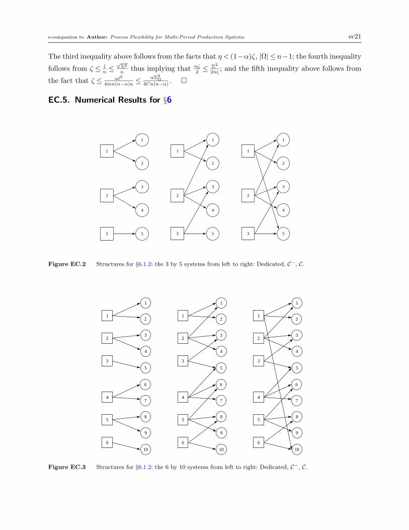
structures with n, m+n− 1 and m+n arcs are displayed in Figure EC.2 (for (m,n) = (3,5)) and
Figure EC.3 (for (m,n) = (6,10)) in Appendix EC.5, and are denoted by D, C− and C, respectively.
D is analogous to the dedicated structure in the balanced system, C can be viewed as a generalized
chaining structure created based on Lemma 3 (using A′ =D) and C− can be viewed as chaining
minus one arc. We note that while C− and C differ by just one arc, they differ significantly in GCG,
leading us to anticipate a significant difference in average backlogs.
Similar to §6.1.1, to understand and compare the effectiveness of C− and C, we compute two
performance measures, R(·) and ∆(·), defined in (50). Recall that R(C) represents the ratio between
the backlog of C and that of full flexibility, and ∆(C) represents the ratio between the improvement
(starting from D) of C and that of full flexibility. The expected backlogs of D, C, C− and full
flexibility are evaluated using methods similar to those in §6.1.1. In Tables EC.4, EC.5 and EC.6,
we present the values of R(C), ∆(C), B(C), R(C−) and ∆(C−) for different system sizes.
The numerical results obtained in non-balanced and asymmetric systems suggest that the struc-
ture C, which contains m+n arcs and has a large GCG, is very effective. In general, the numerical
results in asymmetric systems for C and C− are similar to the numerical results in §6.1.1 for LC and
LC−. For example, with ρ not close to 1, while R(C) is often significantly greater than 1, C always
performs strongly in the measure ∆(·). More specifically, ∆(C) is at least 96.2% for all settings with
ρ= 0.8, and at least 92.3% over all of the tested settings. Also, similar to §6.1.1, the performance
of C deteriorates as the system size increases. Thus, one should expect lower performance of C for
systems with more than 20 plants and products.
Additionally, there is a significant difference between ∆(C) and ∆(C−) computationally, despite
that C and C− only differ by one arc. This confirms the insight we gained from our theoretical
analysis in §4 and §5. That is, for an arbitrary unbalanced and asymmetric system, there exist
systems where it is necessary to have m+n arcs to create effective structures, and m+n− 1 arcs
are typically not enough.
6.2. Continuous-Time Environments
Past literature has observed the effectiveness of chaining in other dynamic environments such as
production lines and call centers (see Hopp et al. (2004), Wallace and Whitt (2005), Iravani et al.
(2005)). Motivated by these observations, we simulate the performances of the long chain in two
different continuous-time environments and compare them with our findings in §6.1. The purpose
of our simulation is not just to reproduce the results in the literature, but also to complement
the previous simulation studies by varying parameters n and ρ. Also, in our simulation, we will
Author: Process Flexibility for Multi-Period Production Systems 35
compute metrics R(·) and ∆(·) for different structures, allowing us to directly compare numerical
results from continuous-time settings with that from discrete-time.
6.2.1. Parallel Queueing Networks. We present the simulation results for long chain in
the continuous-time parallel queueing environment, which is often used to simulate call centers
(see, e.g., Wallace and Whitt (2005)). In the continuous-time parallel queueing environment, we
have n types of customers that arrive continuously according to n mutually independent Poisson
processes. The service time of each customer is distributed exponentially with rate 1, and there are
a total of n servers. Similar to §6.1.1, we assume that the arrival rate is almost symmetric; type 1
customers have arrival rate 0.95ρ, type 2,3, . . . , n−1 customers each have arrival rate ρ, and type n
customers have arrival rate 1.05ρ. The parameters n= 5,10,15 and ρ= 0.8,0.9,0.95,0.975,0.9875.
Finally, to simulate the performance of long chain, we adapt the discrete-time MW policy to the
continuous environment, which, in our case, is equivalent to the longest-queue-first policy where
each idling server serves the longest queue among the customer types it is capable of serving.
In Table EC.7, we present the performance of LC (the long chain) and LC− (the long chain less
arc (n,1)) under different values of n and ρ. For each parameter setting, we simulate the system for
4500 warm-up time units, and then record the queue length for the next 500 time units, for 1000
randomly generated samples. (Note that the number of warm-up time units is much larger here
compared to the discrete-time environment because in each time unit, we see on average a much
smaller number of arrivals.) Same as in §6.1, R(A) represents the ratio between the queue length
of A and that of full flexibility; while ∆(A) represents the ratio between the improvement (starting
from dedicated flexibility) of A and that of full flexibility. Finally, SE% denotes the maximum
value of the standard error percentages among D, LC, LC− and F .
Table EC.7 shows that the performance of LC is significantly better than the performance of
LC− in all tested settings, echoing the observation made in Wallace and Whitt (2005) and Iravani
et al. (2005) in parallel queueing networks. Similar to §6.1, with large n and ρ not close to 1,
while the ratio between the queue length of LC to that of full flexibility is not always close to 1,
the ratio ∆(A) between the improvement of LC to that of full flexibility is almost always better
than 80%, indicating that going from the dedicated structure to LC provides most benefit. Also,
because the performance of LC relative to full flexibility deteriorates as n increases, it implies that
more flexibility than LC may be needed to further improve the system performance when n is
large. This observation resonates with the theoretical findings of Tsitsiklis and Xu (2017), which
shows that to achieve small backlogs, one needs a structure where the average degree for each node
should scale as logn asymptotically when n is large. Finally, compared to the simulation results
in §6.1, we see that the relative performance of LC in continuous parallel queueing networks is
Author: Process Flexibility for Multi-Period Production Systems 36
worse compared to the discrete-time backlogging environments. Intuitively, this is because in the
discrete-time system, arrivals and services can be thought of as being more “synchronized” in each
time period, compared to those in the continuous-time setting, which makes the effectiveness of
LC more pronounced.
6.2.2. Serial Production Line. Next, we present the simulation results for long chain in a
continuous-time serial production line. We simulate an environment that was previously studied
by Hopp et al. (2004), where flexible service stations operate under a constant work-in-process
(CONWIP) release policy. Under this environment, a new job is released into the system only
when a job is completed, hence keeping the total number of work-in-process at some fixed constant.
Each new job requires n stages of processing before completion, where the processing time at each
stage follows an exponential distribution. Similar to §6.1.1 and §6.2, we set the processing rate
for each stage to be almost symmetric; stage 1 has a processing rate of 0.95, stage 2,3, . . . , n− 1
has a processing rate of 1, and stage n has a processing rate of 1.05. In addition, there are n
service stations in the production line. A dedicated flexibility structure under this setting means
that service station i is only capable of processing jobs at stage i, while the long chain structure
has service station i capable of processing jobs at stage i and i+ 1 for i= 1, ..., n− 1, and service
station n is capable of processing jobs at stage n and stage 1. We vary n= 5,10,15 and the number
of work-in-process (wip) n,2n,5n.
To simulate the performance of long chain, we use an adapted MW policy, where each service
station process the longest backlogged stage that it is capable of serving. For each system, we
first run 5000 time units as warm-up times for the system, and then record the number of jobs
completed during the next 5000 time units, for 1000 randomly generated samples. Letting P (A)
denote the average number of jobs completed. We also compute two performance measures:
R(A) =P (A)
P (F), ∆(A) =
P (A)−P (D)
P (F)−P (D), for any flexibility structure A. (51)
where R(A) represents the ratio between the number of jobs processed by A and that of full flexi-
bility, and ∆(A) represents the ratio between the improvement (starting from dedicated flexibility)
of A and that of full flexibility. Contrary to the previous settings, because the number of completed
jobs in full flexibility is greater than that of A, R(A) is less than 1, while ∆(A) is greater than 1.
Table EC.8 presents the performance of LC (the long chain) and LC− (the long chain less arc
(n,1)) under different values of n and the number of work-in-process (wip), measured by R(·) and
∆(·). In the last column of Table EC.8, SE% denotes the maximum standard error percentages
for the average number of jobs processed for dedicated, LC, LC− and full flexibility. There are
some similarities between the performance of LC and LC− in the serial production line to that of
Author: Process Flexibility for Multi-Period Production Systems 37
the parallel queueing environments. In particular, LC significantly outperforms LC− in all tested
settings, and the effectiveness of LC relative to full flexibility seems to deteriorate as n grows. Also,
the effectiveness of LC deteriorates when wip is low. This is intuitive because when wip is low,
service stations under LC will tend to spend more time idling, while full flexibility will not have
service stations idling as long as wip is larger than n.
7. Conclusion and Future Directions
To the best of our knowledge, this paper is the first to theoretically investigate the effectiveness
of sparse flexibility structures in the multi-period systems with finite and unbalanced number
of plants and products. We find that when capacity utilization is high, in order to achieve the
similar performance as full flexibility in the multi-period MTO system, one only needs to design
a sparse flexibility structure with m+ n arcs. Interestingly, we also find that all m+ n arcs are
necessary to guarantee this type of asymptotic performance, as there exist systems that even
the best structure with m+ n− 1 arcs cannot achieve the same asymptotic performance as full
flexibility. In order to verify the robustness of our findings, we performed numerical experiments to
understand the effectiveness chaining (and generalized chaining) structures. In short, the chaining
structure performs very well when benchmarked against dedicated and full flexibility structures
in multi-period make-to-order systems. However, the effectiveness of chaining deterioates as the
system size grows.
To close our paper, we point out several interesting future research avenues. (a) Non-uniform
backlogging costs. We have assumed in this paper that the per-unit backlogging cost is uniform
across different products. The current methodology to establish our results does not readily extend
to the case of non-uniform per-unit backlogging costs. We believe that techniques from, e.g., Ata
and Kumar (2005), which considers non-uniform per-unit backlogging costs, may be combined with
techniques from our paper to establish corresponding results for the case of non-uniform costs. (b)
Production system with inventories. One can also study a production-inventory system where the
firm uses the production resource to accumulate inventories in anticipation of future demand. We
note that if one focus on the stationary base-stock policies suggested by Janakiraman et al. (2014),
then one can view the difference between the inventory level and the base-stock level as “backlog”,
and potentially apply the tools we introduced in this paper. Two interesting open problems in this
direction include, (i) the optimality of base-stock policies in the multi-product system with limited
flexibility; and (ii) the effectiveness of sparse flexible systems under base-stock policies when the
base-stock level is endogenous. (c) Unknown demand rate. The design of flexibility structures with
sufficient GCG requires the knowledge of both the demand rate vector λ and the capacity vector
c. While it is reasonable to expect that most firms have full knowledge of c, estimates of λ can
Author: Process Flexibility for Multi-Period Production Systems 38
be uncertain or inaccurate. Therefore, it is worthwhile investigating the robustness of flexibility
structure with respect to different input demand rates, and the trade-off between sparsity and
inaccurate demand estimates. (d) Finite-period models. Our paper analyzed the infinite-horizon
model. The finite-period flexible production models remain an open and important challenge. Our
simulation suggests that the Max-weight policy with sufficient flexibility can work extremely well
in finite horizon, and it would be very interesting to see any theoretical progress on this front.
Acknowledgments
The authors thank the area editor, the anonymous associate editor, and the anonymous referees for their
constructive and detailed comments, which helped significantly improve both the content and the exposition
of this paper. The research of Cong Shi is partially supported by a National Science Foundation (NSF) grant
CMMI-1634505, and an MCubed grant at the University of Michigan at Ann Arbor.
ReferencesAhuja, R. K., T. L. Magnanti, J. B. Orlin. 1993. Network flows. Prentice Hall, Englewood Cliffs, NJ.
Andradottir, S., H. Ayhan, D. G. Down. 2003. Dynamic server allocation for queueing networks with flexible servers. Operations
Research 51(6) 952–968.
Andradottir, S., H. Ayhan, D. G. Down. 2007. Compensating for failures with flexible servers. Operations Research 55(4)
753–768.
Andradottir, S., H. Ayhan, D. G. Down. 2013. Design principles for flexible systems. Production and Operations Management
22(5) 1144–1156.
Asadpour, A., X. Wang, J. Zhang. 2016. Online resource allocation with limited flexibility. Working Paper, New York University,
NY.
Ata, B., S. Kumar. 2005. Heavy traffic analysis of open processing networks with complete resource pooling: Asymptotic
optimality of discrete review policies. The Annals of Applied Probability 15(1A) 331–391.
Bertsekas, D. P., S. E. Shreve. 2007. Stochastic Optimal Control: The Discrete-Time Case. Athena Scientific, Cambridge, MA.
Bertsimas, D., D. Gamarnik, J. N. Tsitsiklis. 2001. Performance of multiclass markovian queueing networks via piecewise linear
lyapunov functions. Annals of Applied Probability 1384–1428.
Cachon, G., C. Terwiesch. 2011. Matching Supply with Demand: An Introduction to Operations Management . 3rd ed. McGraw-
Hill, Ashland, OH.
Chen, X., T. Ma, J. Zhang, Y. Zhou. 2016. Optimal design of process flexibility for general production systems. Working Paper,
New York University, NY.
Chen, X., J. Zhang, Y. Zhou. 2015. Optimal sparse designs for process flexibility via probabilistic expanders. Operations
Research 63(5) 1159–1176.
Chou, M. C., G. A. Chua, C.-P. Teo, H. Zheng. 2010. Design for process flexibility: Efficiency of the long chain and sparse
structure. Operations Research 58(1) 43–58.
Chou, M. C., G. A. Chua, C.-P. Teo, H. Zheng. 2011. Process flexibility revisited: the graph expander and its applications.
Operations Research 59(5) 1090–1105.
Dai, J. G., W. Lin. 2005. Maximum pressure policies in stochastic processing networks. Operations Research 53(2) 197–218.
Deng, T., Z.-J. M. Shen. 2013. Process flexibility design in unbalanced networks. Manufacturing and Service Operations
Management 15(1) 24–32.
Author: Process Flexibility for Multi-Period Production Systems 39
Desir, A., V. Goyal, Y. Wei, J. Zhang. 2016. Sparse process flexibility designs: Is the long chain really optimal? Operations
Research 64(2) 416–431.
Eryilmaz, A., R. Srikant. 2012. Asymptotically tight steady-state queue length bounds implied by drift conditions. Queueing
Systems 72(3-4) 311–359.
Gurvich, I., W. Whitt. 2009. Scheduling flexible servers with convex delay costs in many-server service systems. Manufacturing
& Service Operations Management 11(2) 237–253.
Hajek, B. 1982. Hitting-time and occupation-time bounds implied by drift analysis with applications. Advances in Applied
probability 502–525.
Harrison, J. M., M. J. Lopez. 1999. Heavy traffic resource pooling in parallel-server systems. Queueing systems 33(4) 339–368.
Hopp, W. J., E. Tekin, M. P. Van Oyen. 2004. Benefits of skill chaining in serial production lines with cross-trained workers.
Management Science 50(1) 83–98.
Iravani, S. M., M. P. Van Oyen, K. T. Sims. 2005. Structural flexibility: A new perspective on the design of manufacturing and
service operations. Management Science 51(2) 151–166.
Janakiraman, G., M. Nagarajan, S. Veeraraghavan. 2014. Simple policies for managing flexible capacity. Working Paper,
University of Texas at Dallas, TX.
Jordan, W., S. Graves. 1995. Principles on the benefits of manufacturing process flexibility. Management Science 41(4) 577–594.
Keslassy, I., N. McKeown. 2001. Analysis of scheduling algorithms that provide 100% throughput in input-queued switches.
Proceedings of the Annual Allerton Conference on Communication Control and Computing, vol. 39. Allerton House,
Monticello, Illinois, 593–602.
Mandelbaum, A., A. L. Stolyar. 2004. Scheduling flexible servers with convex delay costs: Heavy-traffic optimality of the
generalized cµ-rule. Operations Research 52(6) 836–855.
McKeown, N., A. Mekkittikul, V. Anantharam, J. Walrand. 1999. Achieving 100% throughput in an input-queued switch.
IEEE Transactions on Communications 47(8) 1260–1267.
Muller, A., D. Stoyan. 2002. Comparison methods for stochastic models and risks. John Wiley & Sons, Hoboken, New Jersey.
Powell, W. B. 2007. Approximate Dynamic Programming: Solving the curses of dimensionality. John Wiley & Sons, Hoboken,
New Jersey.
Shah, D., D. Wischik. 2012. Switched networks with maximum weight policies: Fluid approximation and multiplicative state
space collapse. The Annals of Applied Probability 22(1) 70–127.
Sheng, L., H. Zheng, Y. Rong, W. T. Huh. 2015. Flexible system design: A perspective from service levels. Operations Research
Letters 43(3) 219–225.
Simchi-Levi, D. 2010. Operations Rules: Delivering Customer Value through Flexible Operations. MIT Press, Cambridge, MA.
Simchi-Levi, D., Y. Wei. 2012. Understanding the performance of the long chain and sparse designs in process flexibility.
Operations Research 60(5) 1125–1141.
Simchi-Levi, D., Y. Wei. 2015. Worst-case analysis of process flexibility designs. Operations Research 63(1) 166–185.
Stolyar, A. L. 2004. Maxweight scheduling in a generalized switch: State space collapse and workload minimization in heavy
traffic. The Annals of Applied Probability 14(1) 1–53.
Tanrisever, F., D. Morrice, D. Morton. 2012. Managing capacity flexibility in make-to-order production environments. European
Journal of Operational Research 216(2) 334–345.
Tassiulas, L., A. Ephremides. 1992. Stability properties of constrained queueing systems and scheduling policies for maximum
throughput in multihop radio networks. IEEE Transactions on Automatic Control 37(12) 1936–1948.
Tsitsiklis, J. N., K. Xu. 2017. Flexible queueing architectures. Operations Research 65(5) 1398–1413.
Wallace, R. B., W. Whitt. 2005. A staffing algorithm for call centers with skill-based routing. Manufacturing & Service
Operations Management 7(4) 276–294.
Author: Process Flexibility for Multi-Period Production Systems 40
Wang, X., J. Zhang. 2015. Process flexibility: A distribution-free bound on the performance of k-chain. Operations Research
63(3) 555–571.
e-companion to Author: Process Flexibility for Multi-Period Production Systems ec1
This page is intentionally blank. Proper e-companion title
page, with INFORMS branding and exact metadata of the
main paper, will be produced by the INFORMS office when
the issue is being assembled.
ec2 e-companion to Author: Process Flexibility for Multi-Period Production Systems
Electronic Companion to
“Process Flexibility for Multi-Period Production Systems”
by Shi, Wei and Zhong
EC.1. Stability Condition
Here, we characterize the conditions on the flexibility structure A, the capacity vector c and the
demand distribution D under which there exists a policy that guarantees the finiteness of the
long-run average backlogging cost. The requirement of finite backlogging cost is also known as the
stability condition, and this consideration motivates us to define the stability of a policy.
Definition EC.1 (Stable Policy). Given a flexibility structure A, plant capacity c, and prod-
uct demand distribution D, a production policy π is said to be stable if the expected long-run
average backlogging costs Γ(π)<∞, and is unstable otherwise.
The following proposition gives a necessary and sufficient condition on c and D for the existence
of a stable policy under A. The proof is standard, and is included here for completeness.
Proposition EC.1. Let the flexibility structure A be given. Then, a necessary and sufficient con-
dition for the existence of a stable policy is
∑Si∈N(Ω)
ci >∑Tj∈Ω
λj, for all Ω⊆ T1, . . . ,Tn, Ω 6= ∅. (EC.1)
Proof of Proposition EC.1. The necessity of (EC.1) can be derived as follows. For any non-
empty subset Ω⊆ T1, . . . ,Tn, the corresponding aggregate demand in time period t is∑Tj∈ΩDj(t),
with E[∑
Tj∈ΩDj(t)]
=∑Tj∈Ω λj, and the maximum production capacity that can be devoted to
this demand is∑Si∈N(Ω) ci. Consider a single-plant production system with capacity
∑Si∈N(Ω) ci
and demand given by∑Tj∈ΩDj(t) in time period t, t = 1,2, · · · . Let Q(t) be the backlog of the
single-plant system at time t, and suppose that this single-plant system starts empty, i.e., Q(0) = 0.
Then, by a standard coupling argument, it can be shown that∑Tj∈ΩBj(t) ≥ Q(t) for each t.
Thus, for the original system to be stable, we need lim sup 1T
∑T
t=1
∑Tj∈ΩBj(t)<∞, and so it is
necessary that lim sup 1T
∑T
t=1Q(t)<∞. To guarantee lim sup 1T
∑T
t=1Q(t)<∞, it is required that∑Si∈N(Ω) ci >
∑Tj∈Ω λj. This establishes necessity.
The sufficiency of (EC.1) can be proved as follows. Suppose that for each non-empty subset
Ω⊆ T1, · · · ,Tn,∑Si∈N(Ω) ci >
∑Tj∈Ω λj. Scale the vector λ by a factor α so that for every non-
empty subset Ω ⊆ T1, · · · ,Tn,∑Si∈N(Ω) ci ≥ α
∑Tj∈Ω λj, and there exists a non-empty subset
Ω⊆ T1, · · · ,Tn such that∑Si∈N(Ω) ci = α
∑Tj∈Ω λj. Necessarily, α> 1. By the max-flow min-cut
e-companion to Author: Process Flexibility for Multi-Period Production Systems ec3
theorem, αλ ∈ R(A). Let π be the production policy that uses the constant schedule αλ. Then,
under the policy π, the system is stable. This concludes the sufficiency part.
An immediate consequence of Proposition EC.1 is the following corollary.
Corollary EC.1. A necessary and sufficient condition for the existence of a stable policy under
the full flexibility structure is Λ<C.
Corollary EC.1 essentially spells out that the weakest condition for the existence of a stable
policy under any given flexibility structure is Λ<C, justifying Equation (3) in Assumption 1.
EC.2. Proofs of Results in §3.2
EC.2.1. Proof of Proposition 1
A key fact that is used in the proof of Proposition 1 is the following lemma.
Lemma EC.1. Let the demand rate vector λ and capacity vector c be given with Λ< C, and λ′
be the projection of λ onto the plane defined by
g |∑n
j=1 gj =C
. Let A be a flexibility structure
that has positive GCG (η > 0). Then, for any x ∈Rn with∑
j xj = 0 and ‖x‖ ≤ η/√n, λ′+ x lies
on the face defined by
g |∑n
j=1 gj =C
, and λ′+ x∈R(A).
Proof of Lemma EC.1. Let x∈Rn be such that∑
j xj = 0 and ‖x‖ ≤ η/√n. Then,
∑j |xj| ≤ η
by the Cauchy-Schwarz inequality. Second, since∑
j xj = 0,∑
j(λ′j + xj) =
∑j λ′j =C, and λ′+ x
lies on the face defined by
g |∑n
j=1 gj =C
. Finally, for any Ω( T1, . . . ,Tn,
∑Tj∈Ω
(λ′j +xj) =∑Tj∈Ω
λ′j +∑Tj∈Ω
xj ≤∑Tj∈Ω
λ′j +∑j
|xj| ≤
∑Si∈N(Ω)
ci− η
+ η=∑
Si∈N(Ω)
ci.
We also note that for each j, λ′j +xj ≥ 0. To see this, for each j, let Ω−j = T1, . . .Tj−1,Tj+1, . . . ,Tn,
and we have
η≤∑
Si∈N(Ω−j)
ci−∑Tj∈Ω−j
λ′j ≤m∑i=1
ci−∑Tj∈Ω−j
λ′j = λ′j.
Thus, we have that λ′j ≥ η ≥ |xj|, implying λ′j +xj ≥ 0. As a result, we can conclude that λ′+ x∈
R(A).
Lemma EC.1 states if A has a positive GCG η, the Euclidean ball defined on the hyperplaneg |∑n
j=1 gj =C
with center λ′ and radius η/√n, lies within the production polytope R(A). The
lemma therefore allows us to connect GCG to the result in Eryilmaz and Srikant (2012), which is
used for the proof of Proposition 1.
ec4 e-companion to Author: Process Flexibility for Multi-Period Production Systems
We first note that the system is stable under the Max-Weight policy. The proof of this fact is
quite standard, by considering the conditional expected drift of the quadratic Lyapunov function∑n
j=1B2j , and invoking the so-called Foster’s lemma. Similar proofs have appeared in e.g., McKeown
et al. (1999), Tassiulas and Ephremides (1992), Dai and Lin (2005). We skip details.
Since the Max-Weight policy is stable, there exists a unique steady-state distribution. Let B(∞)
be the unique random backlog vector in steady state. Furthermore, for any backlog vector B =
(B1,B2, · · · ,Bn), define B = (B1 + B2 + · · · + Bn)/n to be the average of the backlogs, and let
∆B = B− B1, where 1 = (1,1, . . . ,1). Note that ∆B is the vector of deviations of the backlogs
from their average. In addition, we define Dmax as the maximum possible value for the aggregate
demand. Under Assumption 1, we have Dmax ≤ nu.
To prove Proposition 1, we first establish the following state space collapse result. Informally,
state space collapse implies that under the Max-Weight policy, all backlogs Bi stays close to the
mean B, so that the vector ∆B remains small.
Theorem EC.1 (State space collapse). Let B(∞) have the steady-state distribution of the
backlog vector under Max-Weight policy, and flexibility structure A with the GCG η. Then, for any
`∈Z+,
P (‖∆B(∞)‖2 >K ′+ 2ξ`)≤(
ξ
ξ+ γ
)`+1
, (EC.2)
where
K ′ =
(Σ2 +
∑j λ
2j + 2C2
)√n
η; γ =
η
2√n
; ξ =√n(Dmax +C). (EC.3)
Proof of Theorem EC.1. The proof of Theorem EC.1 invokes the following theorem in Bertsi-
mas et al. (2001) (where a weaker version was also given in Hajek (1982)).
Theorem EC.2. Let X(·) be an irreducible, aperiodic and positively recurrent discrete-time
Markov chain with a countable state space X . Suppose that there exists a Lyapunov function
Φ : X →R+ with the following properties.
(a) Bounded increment. There exists a positive constant ξ such that |Φ(X(t+1))−Φ(X(t))| ≤
ξ for all t a.s.
(b) Negative drift. There exist positive constants K ′ and γ such that whenever Φ(X(t))>K ′,
E [Φ(X(t+ 1))−Φ(X(t)) |X(t)]≤−γ. (EC.4)
Then, under the steady-state distribution of X(·), for any `∈Z+,
P (Φ(X)>K ′+ 2ξ`)≤(
ξ
ξ+ γ
)`+1
. (EC.5)
e-companion to Author: Process Flexibility for Multi-Period Production Systems ec5
The proof of Theorem EC.1 then relies on establishing conditions (a) and (b) of Theorem EC.2
for an appropriately chosen Lyapunov function Φ(·). It is straightforward to check that B(·) is
aperiodic and positively recurrent. We also claim that if the product demand instances and plant
capacities are integral (rational), then the state space of B(·) is countable. To see this, note that
the Max-Weight policy solves a network flow problem with integral (rational) input at each time
period, implying that if b(t− 1) and d(t) are integral (rational), then b(t) is integral (rational).
Instead of focusing on the Markov chain B(·), we will consider the closely related chain B′(·),
defined to be B′(t) = B(t) + D(t) for all t.
Proposition EC.2. The following inequality holds for the Lyapunov function Φ(B′) = ‖∆B′‖2.
E [‖∆B′(t+ 1)‖2−‖∆B′(t)‖2 |B′(t)]≤−η√n
+Σ2 +
∑j λ
2j + 2C2
2‖∆B′(t)‖2. (EC.6)
In particular, whenever ‖∆B′(t)‖2 >√n(Σ2+
∑j λ
2j+2C2)
η,
E [‖∆B′(t+ 1)‖2−‖∆B′(t)‖2 |B′(t)]≤−η
2√n. (EC.7)
Proof of Proposition EC.2. The proof of Proposition EC.2 mainly consists of establishing the
A similar identity holds for ‖∆B′(t+ 1)‖22. Therefore, substituting these identities into (EC.11),
we establish (EC.8).
(b) To establish (EC.9), we first write B′(t+ 1) = B′(t)−G(B′(t)) + U(B′(t)) + D(t+ 1). Here
G(B′(t)) is the production schedule used at time t, which depends on the vector B′(t). We use
the following convention here: we suppose that G(B′(t)) is obtained from some (fij)i,j such that∑j fij = ci for all i; i.e., all plants use their production capability fully in each time period. It may
happen that for some j, B′j(t)<Gj(B′(t)), in which case we let Uj(t) =Gj(B
′(t))−B′j(t) be the
unused capacity for product j. Otherwise, let Uj(t) = 0. Then, we denote the vector (Uj(t))j by
U(B′(t)). An immediate consequence is that 〈B(t+1),U(t)〉= 〈B′(t)−G(B′(t))+U(t),U(t)〉= 0.
For notational convenience, we drop the time index, and then
E[‖B′(t+ 1)‖22−‖B′(t)‖22 |B′(t)
]=E
[‖B′−G + U + D‖22−‖B′‖22 |B′
].
We now focus on the term E [‖B′−G + U + D‖22−‖B′‖22 |B′]. We have
E[‖B′−G + U + D‖22−‖B′‖22 |B′
]= E
[‖B′−G + D‖22 |B′
]+E
[‖U‖22 |B′
]+ 2E [〈D,U〉 |B′]−E
[2‖U‖22 |B′
]−E
[‖B′‖22 |B′
]= E [2〈D−G,B′〉 |B′] +E
[‖D−G‖22 |B′
]−E
[‖U‖22 |B′
]+ 2E [〈D,U〉 |B′]
≤ E [2〈D−G,B′〉 |B′] +E[‖D−G‖22 |B′
]+ 2E [〈D,U〉 |B′] , (EC.12)
where the first equality holds because E [〈B′−G,U〉 |B′] =−E [‖U‖22 |B′]. Next, let us start with
E [〈D−G,B′〉 |B′] and observe that
E [〈D−G,B′〉 |B′] = 〈λ−G,B′〉
= 〈λ′−G,B′〉− 〈λ′−λ,B′〉
= 〈λ′−G,B′〉−nζB′.
By the Max-Weight policy, G is chosen from R(A) to maximize the inner product 〈G,B′〉. By
Lemma EC.1, λ′+ η√n· ∆B′
‖∆B′‖ ∈R(A). Therefore, we have
E [〈D−G,B′〉 |B′] = 〈λ′−G,B′〉−nζB′
≤− η√n · ‖∆B′‖
〈∆B′,B′〉−nζB′
e-companion to Author: Process Flexibility for Multi-Period Production Systems ec7
=− η√n · ‖∆B′‖
〈∆B′,∆B′〉−nζB′
=− η√n‖∆B′‖−nζB′. (EC.13)
For the remaining terms, we have
E[‖D−G‖22 |B′
]+ 2E [〈D,U〉 |B′] = E
[∑j
(Dj −Gj)2 |B′
]+ 2E
[∑j
DjUj |B′]
= E
[∑j
D2j +∑j
G2j |B′
]− 2E
[∑j
DjGj |B′]
+ 2E
[∑j
DjUj |B′]
≤ E
[∑j
D2j +∑j
G2j |B′
]≤Σ2 +
∑j
λ2j +C2. (EC.14)
Combining (EC.12), (EC.13) and (EC.14), we have established (EC.9).
(c) To establish (EC.10), we have
E[n(B′(t+ 1)
2−B′(t)
2)|B′(t)
]= E
1
n
(∑j
B′j(t+ 1)
)2
− 1
n
(∑j
B′j(t)
)2 ∣∣∣ B′(t)
=
1
nE
(∑j
(B′j −Gj +Uj +Dj)
)2
−
(∑j
B′j
)2 ∣∣∣ B′
=
2
n
(∑j
B′j
)E
[∑j
(Dj −Gj)∣∣∣ B′
]+
1
nE
(∑j
(Dj −Gj)
)2 ∣∣∣ B′
+
2
nE
[(∑j
(B′j +Dj −Gj)
)(∑j
Uj
)∣∣∣ B′
]
= −2nζB′+1
n
(Σ2 + (Λ−C)2
)+
2
nE
[(∑j
(B′j +Dj)
)(∑j
Uj
)∣∣∣ B′
]− 2C
nE
[∑j
Uj
∣∣∣ B′
]
≥ −2nζB′+1
n
(Σ2 + (Λ−C)2
)− 2C2
n=−2nζB′+
1
n
(Σ2 +n2ζ2− 3C2
).
Combining (EC.9) and (EC.10), we have
E[(‖B′(t+ 1)‖22−‖B′(t)‖22
)−n
(B′(t+ 1)
2−B′(t)
2)∣∣∣ B′(t)
]≤ −2nζB′(t)− 2η√
n‖∆B′(t)‖2 +
(Σ2 +C2 +
∑j
λ2j
)+ 2nζB′(t)− 1
n
(Σ2 +n2ζ2− 3C2
)≤ − 2η√
n‖∆B′(t)‖2 +
(Σ2 + 2C2 +
∑j
λ2j
).
ec8 e-companion to Author: Process Flexibility for Multi-Period Production Systems
Thus, by (EC.8),
E [‖∆B′(t+ 1)‖2−‖∆B′(t)‖2 |B′(t)] ≤1
2‖∆B′(t)‖2
(− 2η√
n‖∆B′(t)‖2 +
(Σ2 + 2C2 +
∑j
λ2j
))
≤ − η√n
+Σ2 +
∑j λ
2j + 2C2
2‖∆B′(t)‖2.
This concludes the proof of Proposition EC.2.
With Proposition EC.2, we can now complete the proof of Theorem EC.1.
Proof of Theorem EC.1. We have already established the negative drift condition (b) (of The-
orem EC.2) in Proposition EC.2. To establish condition (a), first note that