44
Project GAES Environmental Impact of Delay EEC/SEE/2006/006

Project GAESEnvironmental Impact of Delay
EEC/SEE/2006/006

Project GAES - Environmental Impact of Delay This report was prepared for EUROCONTROL Experimental Centre Project GAES by: ENVISA. Author(s): Sandrine Carlier, Jean-Claude Hustache
ENVISA, 38 rue des Gravilliers, 75003, Paris, France Email: [email protected] Web: www.env-isa.com
Frank Jelinek, EUROCONTROL Experimental Centre Review: Rob Dunlop EEC Note : EEC/SEE/2006/006
© European Organisation for the Safety of Air Navigation EUROCONTROL 2006 This document is published by EUROCONTROL in the interest of the exchange of information. It may be copied in whole or in part providing that the copyright notice and disclaimer are included. The information contained in this document may not be modified without prior written permission from EUROCONTROL. EUROCONTROL makes no warranty, either implied or express, for the information contained in this document, neither does it assume any legal liability or responsibility for the accuracy, completeness or usefulness of this information.
Project GAES - Environmental Impact of Delay
EXECUTIVE SUMMARY
General The regulation of air traffic, as currently done by the CFMU and the regional ATFCM cells, mainly relies on a ground delay principle. The CFMU allocates departure slots by delaying on the ground the flights that might encounter congestion at some stage of their trip. This is a preventive strategy based on the idea that avoiding en-route traffic overload contributes to safety and that ground delays should, in theory, be cheaper than their en-route equivalent from the airspace users' viewpoint.
This study is, to our knowledge, the first tentative to do an environmental analysis of ground delays. It seeks to establish orders of magnitudes of the environmental benefits of ground delays compared to their possible substitutes: airborne holding stacks or rerouting of traffic.
Analysis plan The study examined two scenarios, a ground delay scheme based on the current situation, and a hypothetic airborne delay scheme. The ground delay scenario studies the use of 3 energy sources: aircraft engines; auxiliary power units; and ground power units. The airborne delay scenario studies 2 options: holding stacks before arrival; and rerouting to avoid congested sectors.
We concentrated the analysis on the main aircraft types operated at the most congested airports in Europe (Frankfurt, London Heathrow, Zurich, Paris CDG, Wien, Roma Fiumicino, Munchen, Amsterdam, Barcelona, Brussels Zaventem, Madrid, Praha, Iraklion, Villafranca, Alicante, Dublin) and assumed that all flights had the same probability of ATFM delay duration.
In 2004, there were 8.9 million flights in Europe, of which 8.5% were delayed due to ATFM regulations by at least 5 minutes. Among the delayed flights, 54% were delayed between 5 and 15 minutes; 32% between 15 and 30 minutes; 12% between 30 and 60 minutes, and 2% by more than 60 minutes.
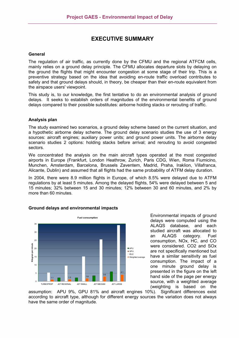
Ground delays and environmental impacts Environmental impacts of ground delays were computed using the ALAQS database, and each studied aircraft was allocated to an ALAQS category. Fuel consumption, NOx, HC, and CO were considered. CO2 and SOx are not specifically mentioned but have a similar sensitivity as fuel consumption. The impact of a one minute ground delay is presented in the figure on the left hand side of the page per energy source, with a weighted average (weighting is based on the
assumption: APU 9%, GPU 81% and aircraft engines 10%). Significant differences exist according to aircraft type, although for different energy sources the variation does not always have the same order of magnitude.
Fuel consumption
1.1 1.3 1.83.0
4.1
0
5
10
15
20
25
30
35
TURBOPROP JET REGIONAL JET SMALL JET MEDIUM JET LARGE
Kilo
gram
per
min
ute
APUGPUIDLEWeighted average
Project GAES - Environmental Impact of Delay
iv EEC/SEE/2006/006
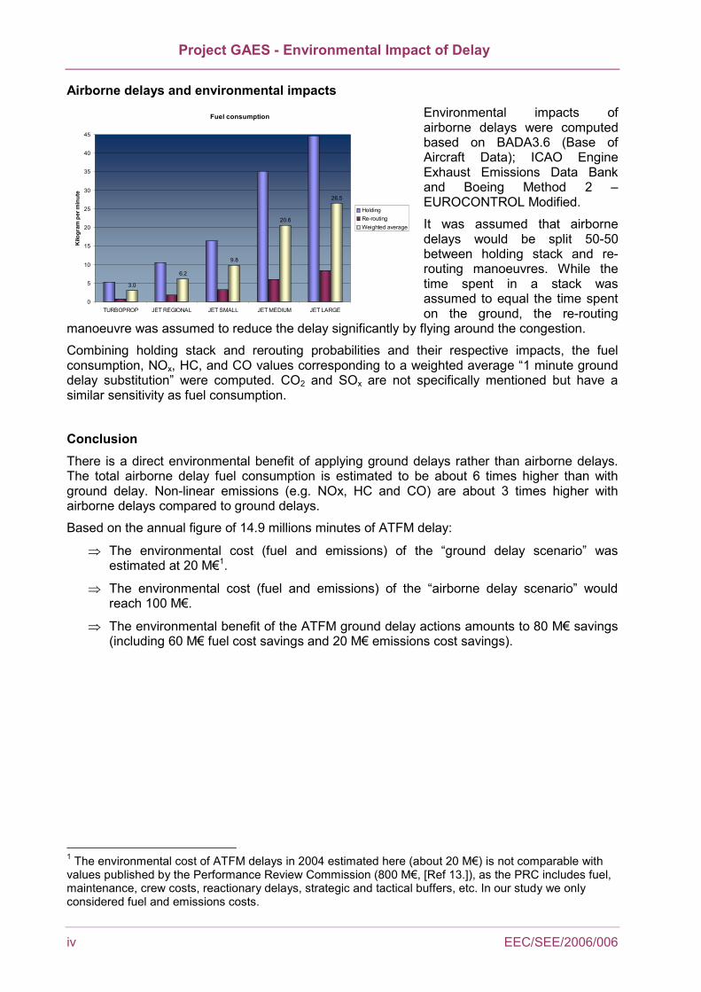
Airborne delays and environmental impacts Environmental impacts of airborne delays were computed based on BADA3.6 (Base of Aircraft Data); ICAO Engine Exhaust Emissions Data Bank and Boeing Method 2 – EUROCONTROL Modified.
It was assumed that airborne delays would be split 50-50 between holding stack and re-routing manoeuvres. While the time spent in a stack was assumed to equal the time spent on the ground, the re-routing
manoeuvre was assumed to reduce the delay significantly by flying around the congestion.
Combining holding stack and rerouting probabilities and their respective impacts, the fuel consumption, NOx, HC, and CO values corresponding to a weighted average “1 minute ground delay substitution” were computed. CO2 and SOx are not specifically mentioned but have a similar sensitivity as fuel consumption.
Conclusion There is a direct environmental benefit of applying ground delays rather than airborne delays. The total airborne delay fuel consumption is estimated to be about 6 times higher than with ground delay. Non-linear emissions (e.g. NOx, HC and CO) are about 3 times higher with airborne delays compared to ground delays.
Based on the annual figure of 14.9 millions minutes of ATFM delay:
⇒ The environmental cost (fuel and emissions) of the “ground delay scenario” was estimated at 20 M€1.
⇒ The environmental cost (fuel and emissions) of the “airborne delay scenario” would reach 100 M€.
⇒ The environmental benefit of the ATFM ground delay actions amounts to 80 M€ savings (including 60 M€ fuel cost savings and 20 M€ emissions cost savings).
1 The environmental cost of ATFM delays in 2004 estimated here (about 20 M€) is not comparable with values published by the Performance Review Commission (800 M€, [Ref 13.]), as the PRC includes fuel, maintenance, crew costs, reactionary delays, strategic and tactical buffers, etc. In our study we only considered fuel and emissions costs.
Fuel consumption
3.0
6.2
9.8
20.6
26.5
0
5
10
15
20
25
30
35
40
45
TURBOPROP JET REGIONAL JET SMALL JET MEDIUM JET LARGE
Kilo
gram
per
min
ute
HoldingRe-routingWeighted average

Project GAES - Environmental Impact of Delay
EEC/SEE/2006/006 v
REPORT DOCUMENTATION PAGE
Reference: SEE Note No. EEC/SEE/2006/006
Security Classification: Unclassified
Originator: ENVISA 38 rue des Gravilliers, 75003, Paris, France www.env-isa.com For Society, Environment, Economy Research Area
Originator (Corporate Author) Name/Location: EUROCONTROL Experimental Centre Centre de Bois des Bordes B.P.15 91222 BRETIGNY SUR ORGE CEDEX France Telephone: +33 1 69 88 75 00
Sponsor: EUROCONTROL EATM
Sponsor (Contract Authority) Name/Location: EUROCONTROL Agency Rue de la Fusée, 96 B –1130 BRUXELLES Telephone: +32 2 729 90 11
TITLE: Environmental Impact of Delay, Project GAES Authors : Sandrine Carlier, Jean-Claude Hustache EEC Contact: Frank Jelinek
Date 09/06
Pages 44
Figures 17
Tables 16
Appendix 2
References 14
EATMP Task Specification -
Project GAES
Task No. Sponsor C21060/02-B156/03
Period Dec. 2005 - March 2006
Distribution Statement: (a) Controlled by: EUROCONTROL Project Manager (b) Special Limitations: None (c) Copy to NTIS: YES / NO Descriptors (keywords): Ground delay – Airborne delay – Holding stack – Rerouting – Speed control – Fuel – Emissions – Environmental cost Abstract: ATFCM activities, coordinated by the CFMU, hold aircraft on ground, preventing these to encounter airborne delays during which fuel is burnt and emissions are produced. On the other hand, during hold-on-ground delays, extended use of A/C engines in idle mode or APU might impact on local air quality. This study is a first attempt to investigate the order of magnitude of the impact of the ATFCM-motivated “hold-on-ground” delays in terms of environmental costs and benefits.

Project GAES - Environmental Impact of Delay
vi EEC/SEE/2006/006
(This page intentionally blank)

Project GAES - Environmental Impact of Delay
EEC/SEE/2006/006 vii
TABLE OF CONTENTS
Table of Contents.................................................................................................... vii
List of Tables.......................................................................................................... viii
List of Figures ........................................................................................................ viii
ABBREVIATIONS ..................................................................................................... ix
1 INTRODUCTION .................................................................................................. 1 1.1 Context ..................................................................................................................................... 1 1.2 Objectives................................................................................................................................. 1 1.3 Approach .................................................................................................................................. 2
2 Definition of scenarios ....................................................................................... 3 2.1 Ground delays .......................................................................................................................... 3 2.2 Airborne delays......................................................................................................................... 3
3 Fleet sample selection and data preparation ................................................... 5 3.1 Fleet selection .......................................................................................................................... 5 3.2 Delay duration per aircraft type ................................................................................................ 7
4 Setting-up the environmental models............................................................... 8 4.1 Ground delays and environmental impacts.............................................................................. 8 4.2 Airborne delays and environmental impacts .......................................................................... 12
5 Computation of local pollution and global emissions for each scenario .... 17 5.1 Annual impact of ground delay – 2004................................................................................... 17 5.2 Potential impact of airborne delay – 2004 equivalent ............................................................ 17 5.3 Comparison of the ground and airborne scenario.................................................................. 18
6 Analysis of results and conversion into financial terms............................... 19 6.1 Fuel unit cost .......................................................................................................................... 19 6.2 Emissions unit cost................................................................................................................. 20 6.3 Comparison of ground and airborne delays environmental costs.......................................... 21 6.4 Synthesis of environmental costs........................................................................................... 24
7 CONCLUSIONS ................................................................................................. 25
8 REFERENCES ................................................................................................... 26
Appendix A ALAQS fuel and Emissions relative to technology................... 27
Appendix B Emission calculation ................................................................... 29

Project GAES - Environmental Impact of Delay
viii EEC/SEE/2006/006
LIST OF TABLES
FIGURE 1: AVERAGE FUEL CONSUMPTION ..................................................................................................... 10 FIGURE 2: AVERAGE NOX EMISSIONS ............................................................................................................... 10 FIGURE 3: AVERAGE HC EMISSIONS ................................................................................................................. 11 FIGURE 4: AVERAGE CO EMISSIONS ................................................................................................................. 11 FIGURE 5: EXAMPLE OF A HOLDING STACK – EXTRACTED FROM PARIS CDG AIP .............................. 13 FIGURE 6: ILLUSTRATION OF REROUTING ASSUMPTIONS.......................................................................... 14 FIGURE 7: AIRBORNE IMPACTS FOR A 1 MINUTE GROUND DELAY AVOIDANCE ................................. 16 FIGURE 8: 2005 “INTO PLANE” JET KEROSENE PRICE – LOW/HIGH SURCHARGE................................... 19 FIGURE 9: CO2 PRICES ON EUA MARKET [REF 12.] ......................................................................................... 20 FIGURE 10: GROUND BASE COST DISTRIBUTION (M€ / YEAR).................................................................... 21 FIGURE 11: AIRBORNE BASE COST DISTRIBUTION (M€ / YEAR) ................................................................ 22 FIGURE 12: FINANCIAL BENEFIT OF GROUND DELAY VS. AIRBORNE DELAY BY POLLUTANT........ 23 FIGURE 13: RELATIVE COST REDUCTION OF GROUND DELAY VS. AIRBORNE DELAY BY
POLLUTANT.......................................................................................................................................... 23 FIGURE 14: IMPACT OF TECHNOLOGY ON FUEL CONSUMPTION .............................................................. 27 FIGURE 15: IMPACT OF TECHNOLOGY ON NOX EMISSIONS ....................................................................... 27 FIGURE 16: IMPACT OF TECHNOLOGY ON HC EMISSIONS .......................................................................... 28 FIGURE 17: IMPACT OF TECHNOLOGY ON CO EMISSIONS .......................................................................... 28
LIST OF FIGURES
TABLE 1: ALLOCATION OF GROUND DELAY PER OPERATING MODE........................................................ 3 TABLE 2: ALLOCATION OF AIRBORNE DELAYS PER OPTION....................................................................... 4 TABLE 3: FLEET SELECTION.................................................................................................................................. 5 TABLE 4: SELECTED AIRCRAFT TYPES............................................................................................................... 6 TABLE 5: 2004 DELAY DISTRIBUTION ................................................................................................................. 7 TABLE 6: ASSUMED PROBABILITY OF DELAY DURATION............................................................................ 7 TABLE 7: APU FUEL AND EMISSION RATES....................................................................................................... 8 TABLE 8: GPU FUEL AND EMISSION RATES....................................................................................................... 9 TABLE 9: ENGINES IN IDLE MODE - FUEL AND EMISSION RATES ............................................................... 9 TABLE 10: ENGINES IN AIRBORNE HOLDING MODE – FUEL AND EMISSION RATES ............................ 13 TABLE 11: ESTIMATED EQUIVALENCE BETWEEN GROUND DELAYS AND REROUTING DURATION15 TABLE 12: ENGINES IN AIRBORNE REROUTING MODE – FUEL AND EMISSION RATES ....................... 15 TABLE 13: ANNUAL IMPACT OF GROUND DELAY ......................................................................................... 17 TABLE 14: ANNUAL IMPACT OF AIRBORNE DELAY...................................................................................... 17 TABLE 15: ANNUAL DIFFERENCE BETWEEN AIRBORNE AND GROUND DELAYS ................................. 18 TABLE 16: EMISSIONS UNIT COSTS (€/TONNE) – LOW, BASE, HIGH .......................................................... 20

Project GAES - Environmental Impact of Delay
EEC/SEE/2006/006 ix
ABBREVIATIONS
AIP Aeronautical Information Publications ALAQS Local Air Quality Modelling Tool & Guidance Material APU Auxiliary Power Unit ATFM Air Traffic Flow Management ATFCM Air Traffic Flow and Capacity Management BADA Base of Aircraft Data CAMES Co-operative ATM Measures for a European Single Sky CFMU Central Flow Management Unit CO Carbon Monoxide CO2 Carbon Dioxide CODA Central Office for Delay Analysis EEC EUROCONTROL Experimental Centre EUA EU Emission Allowances FL Flight level GAES Global Aviation Emission Studies

Project GAES - Environmental Impact of Delay
x EEC/SEE/2006/006
(This page intentionally blank)

Project GAES - Environmental Impact of Delay
EEC/SEE/2006/006 1
1 INTRODUCTION
1.1 Context
Air traffic in Europe is regulated by the CFMU (Central Flow Management Unit), which holds the functions of centralising declared capacities by all European air traffic control centres and declared flight plans by all airspace users operating under Instrument Flight Rules.
By confronting ‘supply of capacity’ and ‘demand for capacity’, the CFMU is able to: strategically and tactically estimate the European air traffic system planed and actual utilisation; ensure smooth operations; avoid controller workload above desired levels; and ensure a fair treatment of airspace users in their access to capacity.
The regulation of air traffic mainly relies on a ground delay principle. The CFMU allocates departure slots by delaying on the ground the flights that might encounter traffic overloads at some stage of the trip. This can be seen as a preventive action, based on the idea that avoiding en-route traffic overload is a safety factor, and that for airspace users, a ground delay should in theory be more economical than an en-route delay.
However, ground delay regulations generate congestion at the departure airport; they also prevent the use of en-route or arrival capacity that would appear to be available in reality although not forecasted at the time of the slot allocation. Depending on the aircraft type, the delay duration, the airline operational organisation and the strategic importance of the delayed flight, it is not obvious that ground delays are always more efficient than en-route delays or vice versa.
One way to approach these issues would be to study delays (airborne and ground) before and after the CFMU creation. However, the CFMU started its operations in March 1996 and replaced a situation where traffic flow management existed but was not centralised. Five flow management cells were operating in Europe: Paris (established in 1973), Frankfurt, London, Roma, and Madrid. Inferring from delay statistics the impact of CFMU regulation is thus not possible, as pre-CFMU times do not mean absence of flow regulation by ground delays. Furthermore, traffic and control centre capacities grew at different speeds over time, and delay statistics, although influenced by regulation strategies, primarily depend on demand / capacity patterns.
1.2 Objectives
The objective of this study is to conduct an environmental and economic assessment of the ground delay practices and of airborne delays alternatives.
This study is, to our knowledge, the first tentative of an environmental analysis of ground delays. As an exploratory research field, the scope of investigations is deliberately focussed on a reduced traffic sample as modelling the environmental cost for all European traffic would be premature, and too detailed for an initial exercise. The following objectives were pursued:
⇒ To obtain orders of magnitudes of environmental costs of different delay strategies (ground vs. airborne) based on simplified but representative traffic samples;
⇒ To assess impacts on local and global emissions;
⇒ To consider only delays resulting from ATFM (Air Traffic Flow Management) regulation.
The study thus does not cover:
⇒ The investigation of the cost of delays that are not related to an environmental impact (crew cost, maintenance, reactionary delays, passengers delay cost, etc.);

Project GAES - Environmental Impact of Delay
2 EEC/SEE/2006/006
⇒ Other environmental aspects of local pollution and global emissions of aircraft (noise, soil and water pollution, contrails, are not within the scope of this study).
1.3 Approach
The study approach includes 5 steps:
⇒ definition of scenarios
⇒ traffic sample selection and data preparation
⇒ setting-up of the environmental simulation tools
⇒ computation of local pollution and global emissions for each scenario
⇒ analysis of results and conversion into financial terms
The organisation of the report follows the different steps of our approach.

Project GAES - Environmental Impact of Delay
EEC/SEE/2006/006 3
2 DEFINITION OF SCENARIOS The study will examine two scenarios: a ground delay scheme, based on the observed current situation, and an airborne delay scheme.
2.1 Ground delays
The scenario of environmental impact under a ground delay scheme has to consider the aircraft operating mode when delayed on the ground. The following possibilities can be used:
⇒ Engines ON while stationary or taxiing2
⇒ Auxiliary power unit (APU) ON
⇒ Ground Power Unit (GPU) ON
The issue when setting assumptions on the operating mode of an aircraft delayed on the ground is that the situation depends on aircraft, airports, and delay duration. Indeed, being delayed ‘on the ground’ can result in extra time at the gate, where GPU or APU can be used, or in extra time off-gate (stationary or taxi) where the main aircraft engines are used.
A study [Ref 1.] relying on detailed investigations, direct airline interviews and data collection, and used as the reference by the Performance Review Commission for costing ATFM delays in Europe [Ref 2.] has proposed the following assumptions and repartition keys to allocate ground ATFM delays into different operating modes.
Table 1: Allocation of ground delay per operating mode
Operating mode Proportion of time spent At gate with GPU only 81% At gate with APU only 9% Off-gate stationary ground or active taxi out 10%
In absence of contradictory evidence, and for consistency with the PRR (Performance Review Reports) framework, the same assumptions are used in this study. The only difference is that the taxi-out and stationary distinction is not applied as the environmental model used (ALAQS) uses the same fuel and emissions values for both modes.
2.2 Airborne delays
The alternative scenario (airborne delay scheme) is also subject to different options. If airspace users were attributed an arrival slot instead of a departure slot (arrival can be arriving at final destination or arriving in the sector generating an ATFM regulation), airspace users would apply one of the three following options:
⇒ Holding stacks
⇒ Rerouting
⇒ Speed control3
2 The emission model used in this study, ALAQS, makes no difference in term of fuel or emissions between the 2 modes “stationary” and “taxiing”. 3 The speed control alternative was not investigated in this study, but would need to be considered if further studies are launched on the subject.
Project GAES - Environmental Impact of Delay
4 EEC/SEE/2006/006
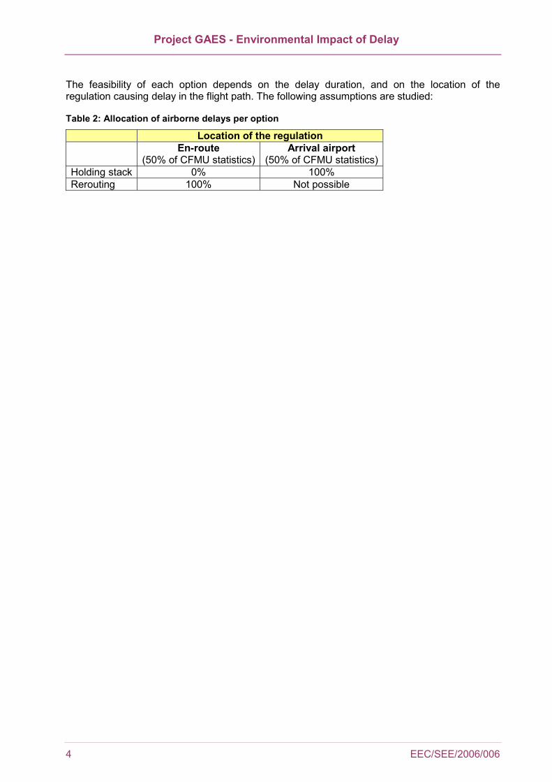
The feasibility of each option depends on the delay duration, and on the location of the regulation causing delay in the flight path. The following assumptions are studied:
Table 2: Allocation of airborne delays per option
Location of the regulation En-route
(50% of CFMU statistics)Arrival airport
(50% of CFMU statistics)Holding stack 0% 100% Rerouting 100% Not possible

Project GAES - Environmental Impact of Delay
EEC/SEE/2006/006 5
3 FLEET SAMPLE SELECTION AND DATA PREPARATION In 2004 there were 14.9 millions minutes of ATFM delays (en-route and airport) in Europe. The following paragraphs explain the selection of a simplified traffic sample representative of the fleet actually suffering from these 14.9 millions minutes of delay.
3.1 Fleet selection
According to [Ref 2.] the most congested airports in Europe are Frankfurt, London Heathrow, Zurich, Paris CDG, Wien, Roma Fiumicino, Munchen, Amsterdam, Barcelona, Brussels Zaventem, Madrid, Praha, Iraklion, Villafranca, Alicante, and Dublin. This group alone generates 80% of European airport delays.
The fleet sample selection is based on the observed fleet of the main airlines operating at these airports, as exposed in Table 3. It does not reflect precisely the whole fleet exposed to en-route delays (this would require the extraction of the information from CFMU data), however, it is assumed that the resulting selection is wide enough to be representative of the fleet suffering en-route congestion, and not only airport delays.
Table 3: Fleet selection4
Lufth
ansa
Brit
ish
Airw
ays
Swis
s
Air
Fran
ce
Aus
tria
n ai
rline
s
grou
p.
Alit
alia
KLM
Iber
ia
Aer
Lin
gus
Oly
mpi
c
Cze
ch
Airl
ines
A300-600 14 1 A310-300 4 A318-100 9 A319-100 20 33 7 45 6 12 7 A320-100 5 12 A320-200 36 21 14 55 8 11 60 20 2
A321-100 4 5 23 A321-200 26 7 8 6 14 6 2
A330-200 2 9 16 3 3 A330-300 8 4 4 A340-300 30 9 20 18 4 A340-600 10 4 9 B717-200 3 B737-300 33 5 14 1 B737-400 18 13 13 15 B737-500 30 9 14 14 B737-800 14 B737-900
9
5 B757-200 13 10
4 Airlines’ fleet information was taken from airlines’ websites and publicly available information.

Project GAES - Environmental Impact of Delay
6 EEC/SEE/2006/006
B767 6 13 B767-300ER 21 B747-200 6 2 B747-300 2 2 B747-400 30 57 16 22 2 B747-200F 9 B747-300ERF 11 B747-400ERF 4 3 B777-200 3 25 10 B777-300 10 B777-200ERF 40
3 10
MD-11 19 2 10 MD-82 76 MD-88 12 MD-87 21 Embraer ERJ 145 8 Avro RJ85 18 4 Avro RJ100 14 CRJ-700 20 CRJ-100/200 41 16 Fokker 70 9 Fokker 100 9 ATR42-300 3 ATR42-400 2 ATR42-500
7 3
ATR72-200 225 6 4 Dash 8 4
From Table 3, it appears relevant to focus the environmental impact analysis on the following subset of 16 aircraft types, shown in Table 4. It includes the main aircraft types and represents the diversity of the fleet in operation. This fleet sample should allow the analysis of different environmental characteristics while keeping a small and workable sample size, flexible enough to run alternative scenarios.
Table 4: Selected aircraft types
A319-100 B747-400 A320-200 B777-200 A321-100 MD-82 A330-200 Avro RJ85 A340-300 CRJ100/200B737-300 ATR42-300 B737-500 ATR72-200 B757-200 B767
5 Austrian Airlines Group has no ATR72, but Bombardier Q aircraft, for which fuel and emissions indices were not available. We thus replaced this aircraft in our calculations by the ATR72.

Project GAES - Environmental Impact of Delay
EEC/SEE/2006/006 7
3.2 Delay duration per aircraft type
Any of the above aircraft can be subject to ATFM regulation of variable duration. It could be derived from CFMU statistics that particular aircraft types are actually suffering longer delays than others depending on the types of routes they operate. However, focusing the analysis at such a level of detail would allow for a precise ex-post assessment, but would not reflect what the situation could be in the future.
Actually, in the hypothetic case where the CFMU would not allocate ground regulations but airborne regulations, it is not sure that the delay duration per aircraft type would have the same distribution as today. It is therefore difficult to infer from observations a precise delay duration distribution pattern. The 2004 distribution is shown for illustration purposes. The current study will model environmental impacts of ground and airborne delays of any duration for all aircraft types.
As stated in [Ref 2.], there were 8.9 million flights in 2004 among which 8.5% (i.e. 756,500 flights) were delayed by at least 5 minutes because of ATFM regulations. The repartition of delays per delay duration is presented in Table 5.
Table 5: 2004 delay distribution
Delay duration [minutes] % total traffic Number of flights
0 – 4 91.4 Not considered delayed5 – 15 4.6 409,40016 – 30 2.7 240,30031 – 60 1.0 89,000> 60 0.2 17,800
We infer from Table 5 that any delayed aircraft is subject to probability of delay duration as shown in Table 6 below (this assumption allows the estimation of the 2004 total delay of 14.9 million minutes):
Table 6: Assumed probability of delay duration
Delay duration [min]
Probability [%]
10 54% 23 32% 45 12% 70 2%

Project GAES - Environmental Impact of Delay
8 EEC/SEE/2006/006
4 SETTING-UP THE ENVIRONMENTAL MODELS
4.1 Ground delays and environmental impacts
Environmental impacts of ground delays are computed using the ALAQS database [Ref 3.], [Ref 4.], [Ref 5.]. The database groups specific aircraft into categories and then allocates fuel and emissions values per category. The list of aircraft selected from Table 3 has the following correspondence with ALAQS categories:
⇒ TURBOPROP - includes the ATR42 and ATR 72
⇒ JET REGIONAL - includes the Avro RJ85, CRJ100, and CRJ200
⇒ JET SMALL - includes the A319, A320, A321, B737-300, B737-500, B757-200 and MD82
⇒ JET MEDIUM - includes the A330 and B767
⇒ JET LARGE - includes the A340, B747, and B777
4.1.1 Auxiliary Power Units
The fuel use and emission rates of APU, according to the ALAQS database [Ref 4.], are presented in Table 7.
As explained previously, it is assumed in this study that ground delays generate APU utilisation in 9% of cases (see Table 1).
Table 7: APU fuel and emission rates
Fuel
[kg/min] NOx
[g/min] HC
[g/min] CO
[g/min] TURBOPROP --------------------- not equipped with APU----------------------- JET REGIONAL 2.1 10.4 0.6 15.6 JET SMALL 2.1 10.4 0.6 15.6 JET MEDIUM 3.3 31.7 1.0 5.0 JET LARGE 5.8 35.0 4.1 61.3
It is important to note that turbo-propeller aircraft are not equipped with APU. When computing the impacts of an ‘average’ minute of ground delays, turbo-propellers are assumed to use their own engines (in idle mode) when other aircraft use their APU; values applied are shown in Table 9.
As an illustration of this table, an A320 with a 20 minute delay will consume 42 kilogram fuel if using the APU.
4.1.2 Ground Power Units
The only available source of fuel use and emission rates of GPU are ALAQS [Ref 4.] and LASPORT [Ref 3.]. These databases do not distinguish GPU fuel consumption and emissions according to aircraft type, although the power supply to a large jet is obviously more important than to a turbo-propeller. Although subject to assumptions and limitations, we had to use the values shown in Table 8. It is assumed in the study that ground delays rely on GPU in 81% of cases (see Table 1).

Project GAES - Environmental Impact of Delay
EEC/SEE/2006/006 9
Table 8: GPU fuel and emission rates
Fuel
[kg/min] NOx
[g/min] HC
[g/min]CO
[g/min]TURBOPROP JET REGIONAL JET SMALL JET MEDIUM JET LARGE
0.2 20.0 2.5 6.7
The GPU fuel consumption for a 20 minutes delay (for an A320) is reduced to 4 kilograms of fuel, about 10 times less than for an APU. However, it should be noted that the environmental performance of GPU over APU is not consistently better. Actually, for regional and small jets, NOx and HC emissions are higher with GPU than with APU.
4.1.3 Engines in idle mode
The fuel use and emission rates of engines in idle mode, according to the ALAQS database, are presented in Table 9. It is assumed in the study that ground delays generate the use of engines in idle mode in 10% of cases.
Table 9: Engines in idle mode - fuel and emission rates
Fuel
[kg/min] NOx
[g/min] HC
[g/min]CO
[g/min]TURBOPROP 5.3 23.2 31.6 119.3JET REGIONAL 9.5 32.6 42.4 363.8JET SMALL 15.1 62.5 28.4 405.2JET MEDIUM 25.5 109.4 100.5 611.9JET LARGE 34.2 150.0 161.3 1033.4
Aircraft engines are optimised for operations at high altitudes and speed, and the idle mode is obviously not efficient compared to APU or GPU. For each aircraft category, the ALAQS database includes different values reflecting the different technology levels, classified “old”, “present”, and “new”. The impact of technology on engines fuel and emissions can be quite high (see appendix A) and the values for the “present” technology were retained.
Using the same illustrative case of an A320 with 20 minutes of ground delay, the consumption in idle mode reaches 300 kilograms, 75 times more than with a GPU, and 7.5 times more than with an APU.
4.1.4 Emissions for a “standard” minute of ground delay
Based on the assumption that GPU are used in most cases (81%), and APU and engines in idle mode, respectively in 9% and 10% of cases, “standard” fuel consumption and emission rates are computed, and presented in Figure 1, Figure 2, Figure 3 and Figure 4. For each aircraft type, the right hand (orange) bar indicates the weighted average value. CO2 and SOx emissions are proportional to fuel.
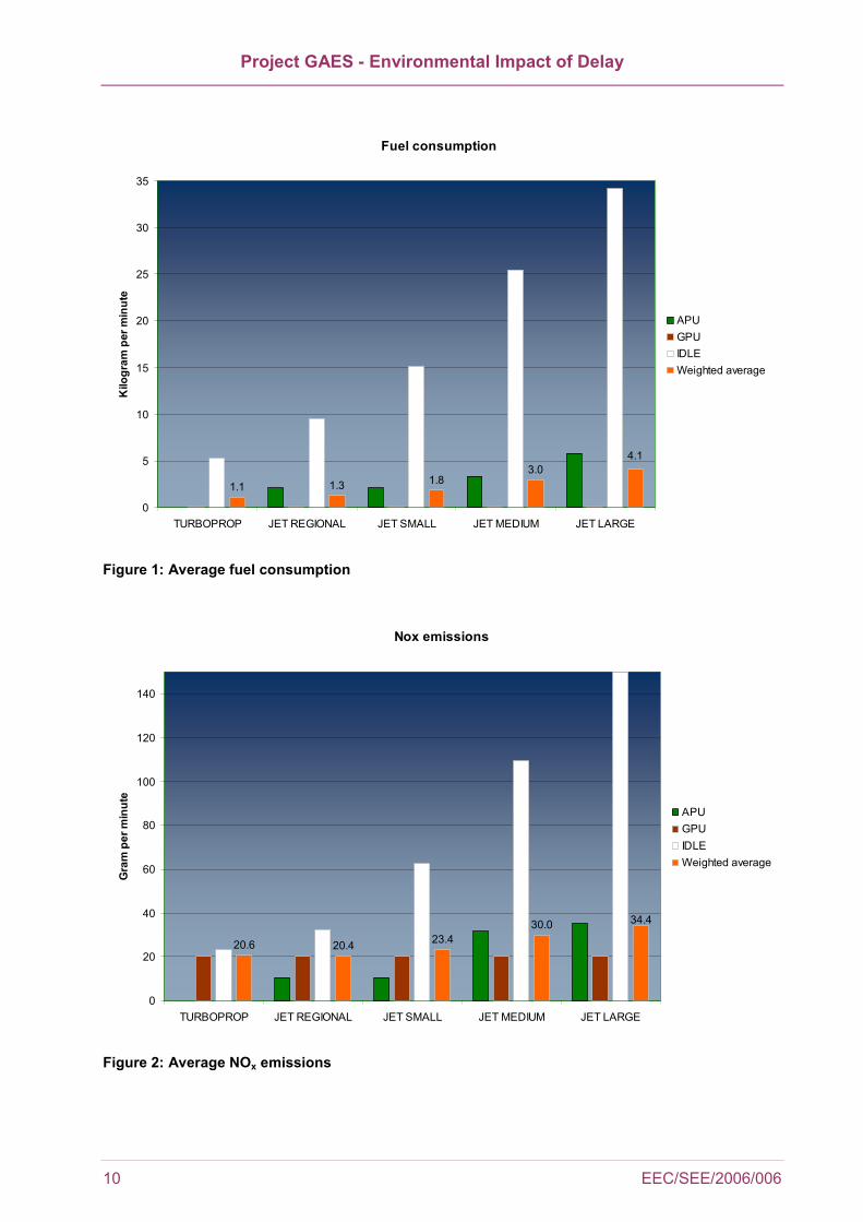
Project GAES - Environmental Impact of Delay
10 EEC/SEE/2006/006
Fuel consumption
1.1 1.3 1.83.0
4.1
0
5
10
15
20
25
30
35
TURBOPROP JET REGIONAL JET SMALL JET MEDIUM JET LARGE
Kilo
gram
per
min
ute
APUGPUIDLEWeighted average
Figure 1: Average fuel consumption
Nox emissions
20.6 20.4 23.430.0 34.4
0
20
40
60
80
100
120
140
TURBOPROP JET REGIONAL JET SMALL JET MEDIUM JET LARGE
Gra
m p
er m
inut
e
APUGPUIDLEWeighted average
Figure 2: Average NOx emissions

Project GAES - Environmental Impact of Delay
EEC/SEE/2006/006 11
HC emissions
8.0 6.3 4.912.2
18.5
0
15
30
45
60
75
90
105
120
135
150
165
TURBOPROP JET REGIONAL JET SMALL JET MEDIUM JET LARGE
Gra
m p
er m
inut
e
APUGPUIDLEWeighted average
Figure 3: Average HC emissions
CO emissions
28.1 43.2 47.3 67.0
114.3
0
150
300
450
600
750
900
1050
TURBOPROP JET REGIONAL JET SMALL JET MEDIUM JET LARGE
Gra
m p
er m
inut
e
APUGPUIDLEWeighted average
Figure 4: Average CO emissions

Project GAES - Environmental Impact of Delay
12 EEC/SEE/2006/006
4.2 Airborne delays and environmental impacts
Environmental impacts of airborne delays are computed based on6:
⇒ BADA3.6 (Base of Aircraft Data) ([Ref 9.]). BADA is an aircraft performance database being maintained and developed by the EUROCONTROL Experimental Centre. Although BADA's main application is trajectory simulation and prediction within ATM, the database holds fuel flow information for 295 different aircraft types.
⇒ ICAO Engine Exhaust Emissions Data Bank ([Ref 6.]). This databank holds results from engine tests. Fuel flow and emission indices for NOx, CO and HC at ground level can be extracted from this databank.
⇒ Boeing Method 2 – EUROCONTROL Modified is applied to adapt ground level emission indices based on altitude.
All the aircraft in Table 4 are modelled by BADA3.6; the most common engine was identified for each of them.
4.2.1 Holding description
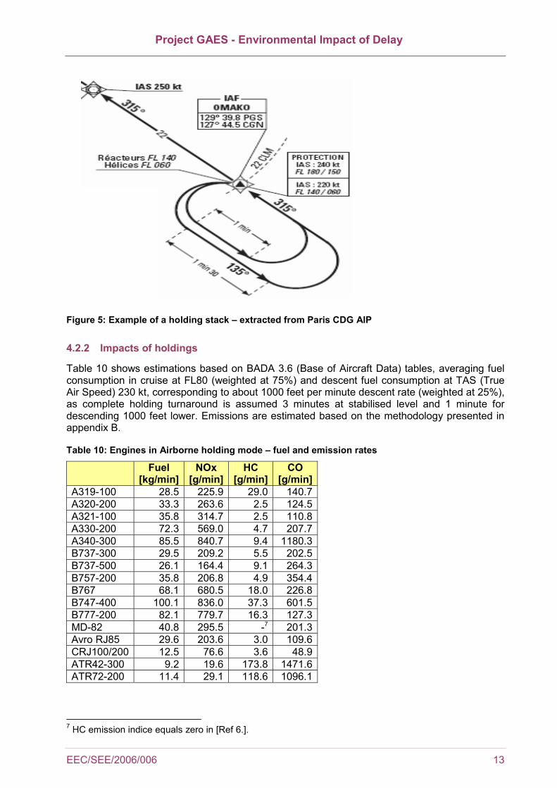
After reviewing the organisation of airborne holding stacks at the main airports presented in paragraph 3.1 (Amsterdam, London, Paris and Zurich), the following assumptions were considered as a reasonable description of the “average” situation, keeping in mind that each airport is specific and that even at a given airport, procedures in holding will vary in accordance with the runway in use, the meteorological conditions, etc.
⇒ The holding stack design is typically based on an oval shape with a lateral leg of 1 minute flight duration, a 180 degrees turn, another 1 minute flight leg, and another 180 degrees turn. The total time for a turnaround is thus assumed to be 4 minutes;
⇒ The exit point of the holding stack (ending the delay) is assumed at FL70;
⇒ The entry point in the stack depends on the traffic already in the queue, knowing that there is a 1000 feet vertical separation between queuing aircraft. One could imagine that for less than 10 minutes delay, the entry point is around FL90, for a 20 minutes delay, FL120, and for a one hour delay, FL220. However differences in fuel consumption between holding stacks starting at FL80 or at FL120, or FL180, are insignificant, and the impact on our results would be negligible. The assumed average altitude for holding stack was set arbitrarily to FL80, ending at FL70.
⇒ The aircraft speed (IAS) in the holding stack is assumed to be 230 kt, knowing that the maximum speed in a TMA (Terminal Manoeuvring Area) is generally 250 kt.
6 Details on the methodology applied is available in 8Appendix B.
Project GAES - Environmental Impact of Delay
EEC/SEE/2006/006 13
Figure 5: Example of a holding stack – extracted from Paris CDG AIP
4.2.2 Impacts of holdings
Table 10 shows estimations based on BADA 3.6 (Base of Aircraft Data) tables, averaging fuel consumption in cruise at FL80 (weighted at 75%) and descent fuel consumption at TAS (True Air Speed) 230 kt, corresponding to about 1000 feet per minute descent rate (weighted at 25%), as complete holding turnaround is assumed 3 minutes at stabilised level and 1 minute for descending 1000 feet lower. Emissions are estimated based on the methodology presented in appendix B.
Table 10: Engines in Airborne holding mode – fuel and emission rates
Fuel [kg/min]
NOx [g/min]
HC [g/min]
CO [g/min]
A319-100 28.5 225.9 29.0 140.7A320-200 33.3 263.6 2.5 124.5A321-100 35.8 314.7 2.5 110.8A330-200 72.3 569.0 4.7 207.7A340-300 85.5 840.7 9.4 1180.3B737-300 29.5 209.2 5.5 202.5B737-500 26.1 164.4 9.1 264.3B757-200 35.8 206.8 4.9 354.4B767 68.1 680.5 18.0 226.8B747-400 100.1 836.0 37.3 601.5B777-200 82.1 779.7 16.3 127.3MD-82 40.8 295.5 -7 201.3Avro RJ85 29.6 203.6 3.0 109.6CRJ100/200 12.5 76.6 3.6 48.9ATR42-300 9.2 19.6 173.8 1471.6ATR72-200 11.4 29.1 118.6 1096.1
7 HC emission indice equals zero in [Ref 6.].

Project GAES - Environmental Impact of Delay
14 EEC/SEE/2006/006
4.2.3 Flight rerouting
The flight rerouting alternative is established based on the assumption that congested sectors are all located in the upper airspace, where aircraft are at standard cruise altitudes. A more precise evaluation of the alternative would require identifying the average altitudes of actual congested sectors. This would probably identify situations were the congested area is an approach sector which is not possible to avoid. Some congested sectors could also appear to be in the ascending phase, where the fuel consumption is higher than in the cruise phase, but it could also be in the descending phase where the consumption is lower. As an initial feasibility study, we consider that setting the assumption at the cruise level will be enough to establish orders of magnitude.
Avoiding a 10 minute ground regulation through a rerouting manoeuvre may not translate into an extra 10 minutes of flight duration. Provided there is just one congested sector the extra flight duration will just be the extra time to fly around the congested sector. However, it is reasonable to assume that for long ATFM delays, there might be a combination of several congested points.
Real sectors are complex polygons, and modelling them in the scope of this study would require too many details to be adjusted with regard to the aim of the study. Computing the extra distance needed to avoid a congested sector is therefore based on the following simplified assumptions:
⇒ Sectors are squares of 100 kilometres side
⇒ Aircraft transit sectors completely, and take about 9 minutes to do so
⇒ On average, the closest detour route from the sector entry point is 50 kilometres (half of the average transit distance)
Departure
Arrival
Total distance without congestion = 500 to 1000 km
Congested sectorAverage transit time = 9 minAverage transit distance = 100 km
Average distance between entry point and closest outbound = 50 km
Departure
Arrival
Total distance without congestion = 500 to 1000 km
Congested sectorAverage transit time = 9 minAverage transit distance = 100 km
Average distance between entry point and closest outbound = 50 km
Figure 6: Illustration of rerouting assumptions
Based on the above assumptions, the extra flight time for avoiding an average congested sector, would be very limited, 1 to 3 minutes only, depending on the congested sector location.
We assume that in case of long ground delays (45 and 70 minutes), there is more than one congested sector to avoid. In the case of 45 minute delays, we assume that 2 sectors have to be avoided leading to 2-6 minutes airborne delay, and 70 minute delays would correspond to 3 congested sectors, and 3 to 9 minutes airborne delay. Because rerouting may generate
Project GAES - Environmental Impact of Delay
EEC/SEE/2006/006 15
congestions in adjacent sectors, a ripple effect may have to be added. This aspect is beyond the scope of the current study, and would need further investigation for a more detailed impact assessment.
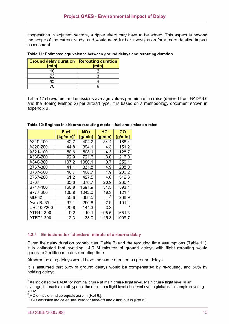
Table 11: Estimated equivalence between ground delays and rerouting duration
Ground delay duration [min]
Rerouting duration[min]
10 2 23 3 45 4 70 6
Table 12 shows fuel and emissions average values per minute in cruise (derived from BADA3.6 and the Boeing Method 2) per aircraft type. It is based on a methodology document shown in appendix B.
Table 12: Engines in airborne rerouting mode – fuel and emission rates
Fuel [kg/min]8
NOx [g/min]
HC [g/min]
CO [g/min]
A319-100 42.7 404.2 34.4 168.4A320-200 44.8 394.1 4.3 151.2A321-100 50.6 508.1 4.3 128.7A330-200 92.9 721.6 3.0 216.0A340-300 107.2 1086.1 9.7 250.1B737-300 41.1 331.8 4.9 205.0B737-500 46.7 408.7 4.9 200.2B757-200 61.2 427.5 4.6 312.3B767 85.8 878.7 20.9 266.1B747-400 160.8 1691.9 31.5 593.1B777-200 105.8 1042.0 16.3 121.4MD-82 50.8 368.5 -9 238.9Avro RJ85 37.1 266.8 2.9 101.4CRJ100/200 20.6 144.3 3.3 -10
ATR42-300 9.2 19.1 195.5 1651.3ATR72-200 12.3 33.0 115.3 1099.7
4.2.4 Emissions for ‘standard’ minute of airborne delay
Given the delay duration probabilities (Table 6) and the rerouting time assumptions (Table 11), it is estimated that avoiding 14.9 M minutes of ground delays with flight rerouting would generate 2 million minutes rerouting time.
Airborne holding delays would have the same duration as ground delays.
It is assumed that 50% of ground delays would be compensated by re-routing, and 50% by holding delays. 8 As indicated by BADA for nominal cruise at main cruise flight level. Main cruise flight level is an average, for each aircraft type, of the maximum flight level observed over a global data sample covering 2002. 9 HC emission indice equals zero in [Ref 6.]. 10 CO emission indice equals zero for take-off and climb out in [Ref 6.].

Project GAES - Environmental Impact of Delay
16 EEC/SEE/2006/006
Figure 7 indicates the impact of airborne holding and rerouting. The "average situation" is plotted on the same graphs. CO2, H2O and SOx emissions are proportional to fuel.
Figure 7: Airborne impacts for a 1 minute ground delay avoidance
Although rerouting fuel flows are higher than for holding, rerouting’s duration is much lower. This results in a reduced impact on the environment due to rerouting as compared to holding stack situation.
With the exception of turboprops, the variation of aircraft type fuel burn and emissions is consistent with ground delays findings: fuel burn and emissions grow with the aircraft size, with the exception of HC and CO emissions which are proportionally more important for turboprops.
Turboprops show the lowest fuel burn and NOx emission rates. On the other hand, HC and CO emissions are much higher than observed for jets. Nevertheless Boeing Method 2 (appendix B) is not designed for turboprops and thus less adapted than for jet engines. Therefore the estimation of HC and CO for turboprops may not reach the same level of accuracy as for other aircraft categories, especially when addressing low power situations.

Project GAES - Environmental Impact of Delay
EEC/SEE/2006/006 17
5 COMPUTATION OF LOCAL POLLUTION AND GLOBAL EMISSIONS FOR EACH SCENARIO
5.1 Annual impact of ground delay – 2004
Based on the annual figure of 14.9 million minutes of ATFM delay in 2004, Table 13 shows the impact, for each aircraft category, of what the fuel consumption and emissions are based on the proportion of each category in the total European air traffic.
Table 13: Annual impact of ground delay
% in flight movement
s
Fuel [tonnes/year
]
NOx [tonnes/year
]
HC [tonnes/year
]
CO [tonnes/year
] JET SMALL 57% 15 465 197 41 399 JET MEDIUM 4% 1 637 16 7 37 JET LARGE 3% 2 049 17 9 57 JET REGIONAL 13% 2 560 41 13 87 TURBOPROP 23% 3 886 70 27 96 TOTAL 100% 25 597 342 98 676
The total environmental impact of ground delay is given on the last row.
5.2 Potential impact of airborne delay – 2004 equivalent
Management of airborne delays would be very dependant on local practices and cannot be generalized. Our main assumption was that a "standard" airborne delay would be equally shared between holdings and flight rerouting.
In absence of ground regulation, airborne delay during 2004 would correspond to 8.511 million minutes. Based on the same presentation as section 5.1, the annual impact of airborne delay is presented in Table 14.
Table 14: Annual impact of airborne delay
% in flight movements
Fuel [tonnes/year]
NOx [tonnes/year]
HC [tonnes/year]
CO [tonnes/year]
JET SMALL 57% 95 260 714 25 550JET MEDIUM 4% 13 981 125 2 42JET LARGE 3% 13 516 126 3 87JET REGIONAL 13% 13 761 93 2 51TURBOPROP 23% 11 911 29 153 1 363TOTAL 100% 148 429 1 087 185 2 093
11 Assumption: 14.9 millions minutes of ATFM delay in 2004 are equivalent to 7.5 million minutes spend in holding stacks plus 1 million minutes of rerouting (see Table 6 and Table 11).
Project GAES - Environmental Impact of Delay
18 EEC/SEE/2006/006
5.3 Comparison of the ground and airborne scenario
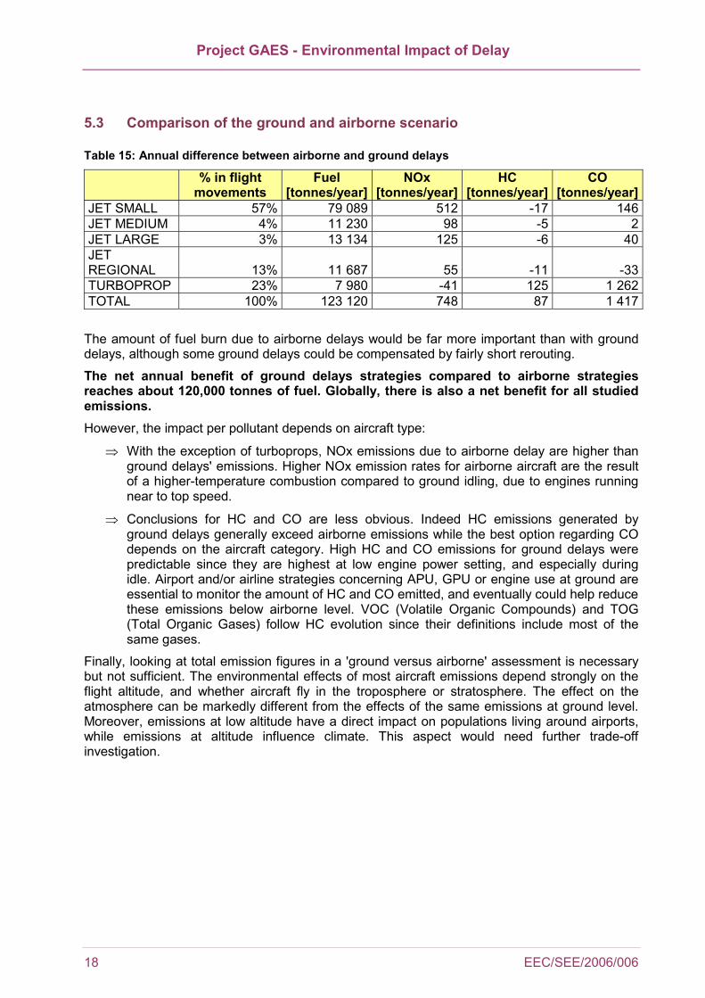
Table 15: Annual difference between airborne and ground delays
% in flight movements
Fuel [tonnes/year]
NOx [tonnes/year]
HC [tonnes/year]
CO [tonnes/year]
JET SMALL 57% 79 089 512 -17 146JET MEDIUM 4% 11 230 98 -5 2JET LARGE 3% 13 134 125 -6 40JET REGIONAL 13% 11 687 55 -11 -33TURBOPROP 23% 7 980 -41 125 1 262TOTAL 100% 123 120 748 87 1 417
The amount of fuel burn due to airborne delays would be far more important than with ground delays, although some ground delays could be compensated by fairly short rerouting.
The net annual benefit of ground delays strategies compared to airborne strategies reaches about 120,000 tonnes of fuel. Globally, there is also a net benefit for all studied emissions. However, the impact per pollutant depends on aircraft type:
⇒ With the exception of turboprops, NOx emissions due to airborne delay are higher than ground delays' emissions. Higher NOx emission rates for airborne aircraft are the result of a higher-temperature combustion compared to ground idling, due to engines running near to top speed.
⇒ Conclusions for HC and CO are less obvious. Indeed HC emissions generated by ground delays generally exceed airborne emissions while the best option regarding CO depends on the aircraft category. High HC and CO emissions for ground delays were predictable since they are highest at low engine power setting, and especially during idle. Airport and/or airline strategies concerning APU, GPU or engine use at ground are essential to monitor the amount of HC and CO emitted, and eventually could help reduce these emissions below airborne level. VOC (Volatile Organic Compounds) and TOG (Total Organic Gases) follow HC evolution since their definitions include most of the same gases.
Finally, looking at total emission figures in a 'ground versus airborne' assessment is necessary but not sufficient. The environmental effects of most aircraft emissions depend strongly on the flight altitude, and whether aircraft fly in the troposphere or stratosphere. The effect on the atmosphere can be markedly different from the effects of the same emissions at ground level. Moreover, emissions at low altitude have a direct impact on populations living around airports, while emissions at altitude influence climate. This aspect would need further trade-off investigation.
Project GAES - Environmental Impact of Delay
EEC/SEE/2006/006 19
6 ANALYSIS OF RESULTS AND CONVERSION INTO FINANCIAL TERMS
In this section, the results of Section 5 are converted into monetary terms using statistics of jet kerosene cost, and results from a previous study on aviation emission costs [Ref 10.]. Additional emission cost information was derived from the 2002 report by CE Delft on external costs of aviation [Ref 11.], and from the EU Emission Allowances (EUA) market [Ref 12.].
The objective is to quantify the financial benefit of delaying aircraft on the ground compared to delaying them en-route.
6.1 Fuel unit cost
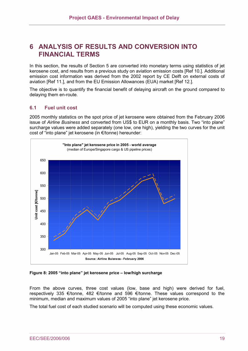
2005 monthly statistics on the spot price of jet kerosene were obtained from the February 2006 issue of Airline Business and converted from US$ to EUR on a monthly basis. Two “into plane” surcharge values were added separately (one low, one high), yielding the two curves for the unit cost of “into plane” jet kerosene (in €/tonne) hereunder:
"Into plane" jet kerosene price in 2005 - world average(median of Europe/Singapore cargo & US pipeline prices)
300
350
400
450
500
550
600
650
Jan-05 Feb-05 Mar-05 Apr-05 May-05 Jun-05 Jul-05 Aug-05 Sep-05 Oct-05 Nov-05 Dec-05
Source: Airline Buisness - February 2006
Uni
t cos
t [€/
tonn
e]
Figure 8: 2005 “into plane” jet kerosene price – low/high surcharge
From the above curves, three cost values (low, base and high) were derived for fuel, respectively 335 €/tonne, 482 €/tonne and 596 €/tonne. These values correspond to the minimum, median and maximum values of 2005 “into plane” jet kerosene price.
The total fuel cost of each studied scenario will be computed using these economic values.

Project GAES - Environmental Impact of Delay
20 EEC/SEE/2006/006
6.2 Emissions unit cost
For each pollutant, a low, base and high unit cost was derived from a literature review. The unit costs of CO2, NOx, SOx, HC and CO were taken from a study on aviation emission costs [Ref 10.], while H2O prices were taken from the 2002 CE Delft report [Ref 11.].
Table 16: Emissions unit costs (€/tonne) – Low, Base, High
Unit Costs (€/tonne) Low Base High CO2 11 37 65H2O 2.8 8.3 14NOx 4,460 6,414 10,693SOx 2,110 6,094 11,133HC 2,569 5,543 8,518CO 104 142 205
It was initially attempted to obtain different unit costs for ground emissions on one hand and airborne emissions on the other hand. Indeed, the impact of a given pollutant on the environment depends on the altitude at which it has been emitted.
Such information could only be partially obtained, therefore a single value was used in the scope of this study. As far as NOx is concerned, the level of uncertainty for both local and global costs is such that average values are finally not very different. Furthermore, the cost of ground emissions is highly dependent on the population density around the airport – which is an unknown parameter in the present study. Later in this section it will be discussed which pollutants should actually be taken into account in the ground scenario, and which ones should be considered in the airborne scenario.
In addition to the above literature review, recent statistics of CO2 prices on the EU Emission Allowances (EUA) market were collected. The corresponding evolution of CO2 price along 2004 and 2005 is represented hereunder:
Figure 9: CO2 prices on EUA market [Ref 12.]

Project GAES - Environmental Impact of Delay
EEC/SEE/2006/006 21
The above graph shows CO2 values that are comparable to those in Table 16. However, it tends to show as well that the high value in Table 16 may be overestimated when assessing the cost of ground-emitted CO2
12.
6.3 Comparison of ground and airborne delays environmental costs
From the emission amounts in Table 13 and Table 14, and the unit costs in previous sections, environmental costs of ground and airborne delays were calculated.
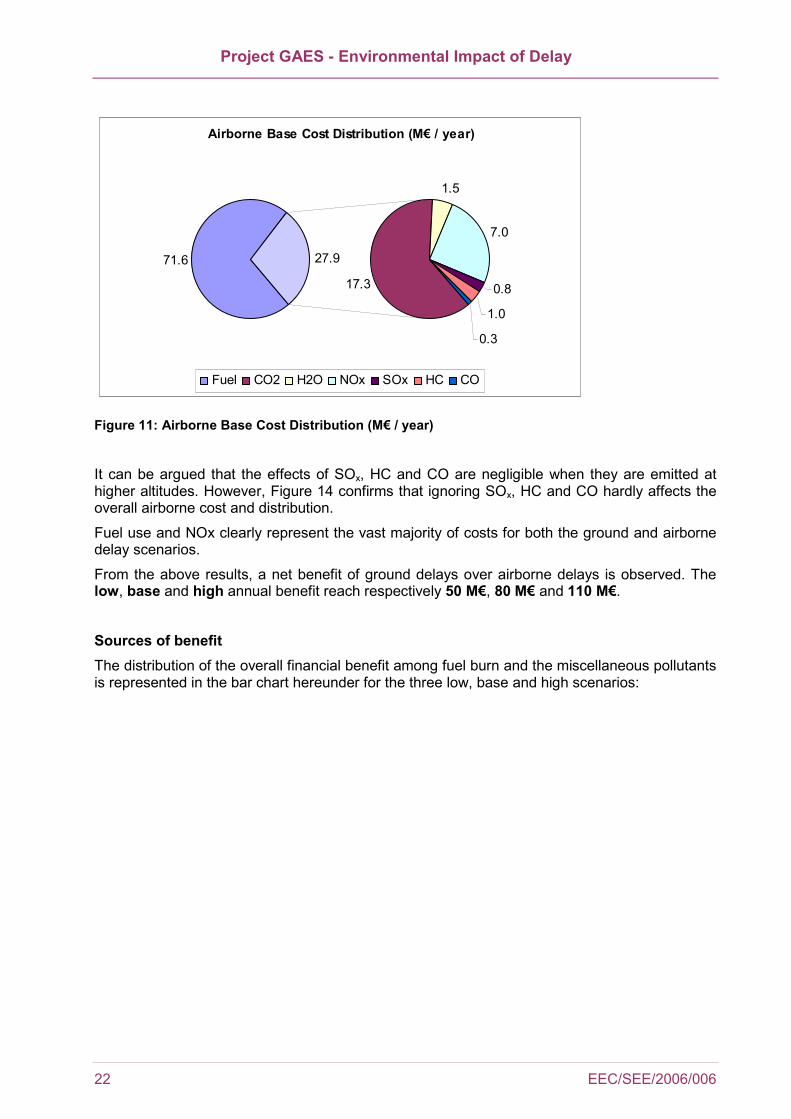
When taking all fuel use and pollutants into account, the yearly environmental cost of ground delay has low, base and high values of about 10 M€, 20 M€ and 25 M€ respectively13. The ground base cost distribution among fuel and emissions is represented in the pie chart hereafter:
Ground Base Cost Distribution (M€ / year)
12.3
3.0
0.3 2.2
0.1
0.5
0.1
6.2
Fuel CO2 H2O NOx SOx HC CO
Figure 10: Ground Base Cost Distribution (M€ / year)
It can be argued that the effect of ground-emitted H2O is null, and therefore the associated cost should be ignored. However, Figure 10 shows that ignoring H2O hardly affects the overall ground cost and distribution. The environmental cost of ground delay could be further reduced if low, base and high CO2 prices correlated with the recent values on the EUA.
When taking all fuel use and pollutants into account, the yearly cost of airborne delay has low, base and high values of 60 M€, 100 M€ and 135 M€ respectively. The base cost distribution among fuel and emissions is represented in the pie chart hereafter:
12 This assumes that the market cost of CO2 credits equals the cost impact on the environment. This is debatable, as this market cost only reflects how much companies are willing to pay to avoid reducing CO2. 13 The environmental cost of ATFM delays in 2004 estimated here (about 20 M€) is not comparable with values published by the Performance Review Commission (800 M€, [Ref 13.]), as the PRC includes fuel, maintenance, crew costs, reactionary delays, strategic and tactical buffers, etc. In our study we only looked at fuel and emissions costs.
Project GAES - Environmental Impact of Delay
22 EEC/SEE/2006/006
Airborne Base Cost Distribution (M€ / year)
71.6
17.3
1.5
7.0
0.8
1.0
0.3
27.9
Fuel CO2 H2O NOx SOx HC CO
Figure 11: Airborne Base Cost Distribution (M€ / year)
It can be argued that the effects of SOx, HC and CO are negligible when they are emitted at higher altitudes. However, Figure 14 confirms that ignoring SOx, HC and CO hardly affects the overall airborne cost and distribution.
Fuel use and NOx clearly represent the vast majority of costs for both the ground and airborne delay scenarios.
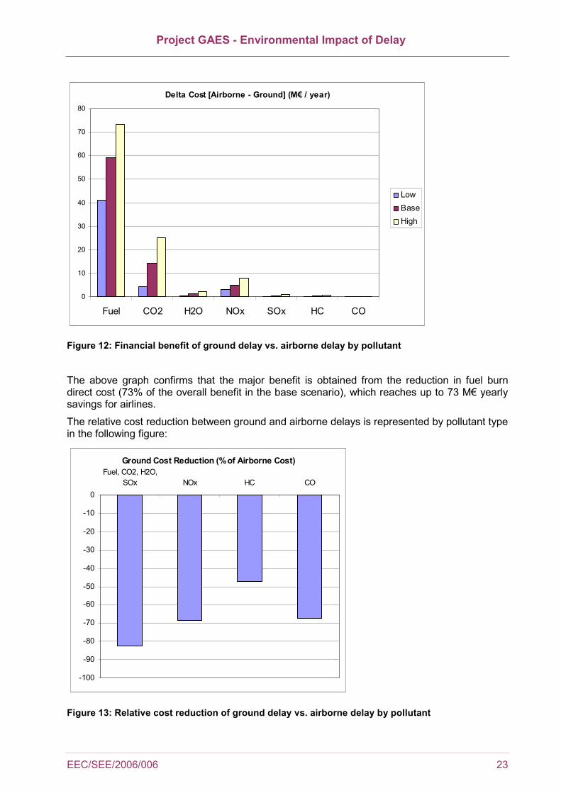
From the above results, a net benefit of ground delays over airborne delays is observed. The low, base and high annual benefit reach respectively 50 M€, 80 M€ and 110 M€.
Sources of benefit The distribution of the overall financial benefit among fuel burn and the miscellaneous pollutants is represented in the bar chart hereunder for the three low, base and high scenarios:
Project GAES - Environmental Impact of Delay
EEC/SEE/2006/006 23
Delta Cost [Airborne - Ground] (M€ / year)
0
10
20
30
40
50
60
70
80
Fuel CO2 H2O NOx SOx HC CO
LowBaseHigh
Figure 12: Financial benefit of ground delay vs. airborne delay by pollutant
The above graph confirms that the major benefit is obtained from the reduction in fuel burn direct cost (73% of the overall benefit in the base scenario), which reaches up to 73 M€ yearly savings for airlines.
The relative cost reduction between ground and airborne delays is represented by pollutant type in the following figure:
Ground Cost Reduction (% of Airborne Cost)
-100
-90
-80
-70
-60
-50
-40
-30
-20
-10
0
Fuel, CO2, H2O,SOx NOx HC CO
Figure 13: Relative cost reduction of ground delay vs. airborne delay by pollutant
Project GAES - Environmental Impact of Delay
24 EEC/SEE/2006/006
Figure 13 shows that the maximum relative gain between the airborne and ground delay scenarios is also obtained for fuel (83% reduction) in terms of both the emitted mass and its cost. The same figure applies to CO2, H2O and SOx as their masses are proportional to the fuel burn mass.
Sensitivity analysis When:
⇒ H2O is ignored in ground emissions,
⇒ SOx, HC, CO are ignored in airborne emissions,
⇒ and the cost of ground-emitted CO2 is updated to the EUA market prices (low/base/high vales of 10/20/30 €/tonne – see Figure 9),
the resulting financial benefit remains very similar: 50 M€, 80 M€ and 110 M€ for low, base, high estimations respectively.
6.4 Synthesis of environmental costs
The financial assessment of the ground delay benefits compared to airborne delay shows a gain of around 80 M€ per year when the base unit costs are used for fuel and emissions.
From these 80 M€, around 60 M€ are related to the reduction in fuel consumption – which represents a direct benefit for airlines, while the remaining 20 M€ stand for the indirect cost of emissions, essentially CO2 and NOx (14 M€ and 5 M€ respectively).
Confidence in these cost estimations should be fairly high, as the most uncertain unit values are for the pollutant which are the most negligible.
Project GAES - Environmental Impact of Delay
EEC/SEE/2006/006 25
7 CONCLUSIONS This study is the first attempt at quantifying environmental impacts of delays. Initial estimates show that the impact of ground delays is highly dependent on the power source used during the delay. They show as well that the impact of ground delays is less than for airborne delays, both for fuel consumption and emissions.
For all aircraft types GPU are more efficient than APU, and both are far more efficient than aircraft engines in idle mode. A weighting of the different operating modes showed that the fuel consumption during a 1 minute ground delay is between 1kg to 4 kg, depending on aircraft types (see Figure 1).
In absence of ground regulation the 14.9 million minutes ground delays would translate into both:
⇒ 7.5 million minutes spent in holding stacks (around FL100) where aircraft consumption is between 10 and 100 kg/min.
⇒ 1 million minutes of rerouting manoeuvres in order to avoid congested sectors, where aircraft consumption is between 10 and 160 kg/min.
There is a direct environmental benefit of applying ground delays rather than airborne delay. The total airborne delay fuel consumption is estimated to be about 6 times higher than with ground delay. Non-linear emissions (e.g. NOx, HC and CO) are about 3 times higher with airborne delay compared to ground delays.
Based on the annual figure of 14.9 millions minutes of ATFM delay:
⇒ the environmental cost (fuel and emissions) of the “ground delay scenario” was estimated at 20 M€.
⇒ the environmental cost (fuel and emissions) of the “airborne delay scenario” would reach 100 M€.
The environmental benefit of the ATFM ground delay actions therefore amounts to 80 M€ (including 60 M€ fuel cost savings and 20 M€ emissions cost savings).

Project GAES - Environmental Impact of Delay
26 EEC/SEE/2006/006
8 REFERENCES
[Ref 1.] University of Westminster, Transport Studies Group (2004) Evaluating the true cost to airlines of one minute of airborne or ground delay.
[Ref 2.] EUROCONTROL (2005) ATFM and Capacity report 2004.
[Ref 3.] Janicke Consulting, LASPORT version 1.5, 2005, Dunum (Germany)
[Ref 4.] EUROCONTROL, ALAQS-AV Concept Document, working paper
[Ref 5.] FAA, Emission and Dispersion Modeling System User's Manual cersion 4.3, 2005, Washington, DC.
[Ref 6.] ICAO Engine Exhaust Emissions Data Bank; ICAO; Internet Issue 14 (June 2005)
[Ref 7.] JP Airline-Fleets International Aviation Database – BUCHair UK ltd (2004)
[Ref 8.] Scheduled Civil Aircraft Emission Inventory for 1992: Database Development and Analysis; April 1996; NASA LRC; Contractor Report 4700; Steven L. Baughcum, Terrance G. Tritz, Stephen C. Henderson, David C. Picket
[Ref 9.] http://www.eurocontrol.int/eec/public/standard_page/ACE_bada.html
[Ref 10.] ENV-ISA, Environmentally Sustainable Airport Operations, Emissions cost database work package (final version), June 2004.
[Ref 11.] CE Delft, External Costs of Aviation, J.M.W Dings, R.C.N. Wit, B.A. Leurs, M.D. Davidson, W. Fransen, February 2002.
[Ref 12.] Energy Research Centre of the Netherlands (ECN), CO2 Price Dynamics – A Follow-Up Analysis of the Implications of EU Emissions Trading for the Price of Electricity, J.P.M Sijm, Y. Chen, M. Ten Donkelaar, J.S. Hers, M.J.J. Scheepers, March 2006.
[Ref 13.] EUROCONTROL, Eighth Performance Review Report (PRR8) – An Assessment of Air Traffic Management in Europe during the Calendar Year 2004, Performance Review Commission, April 2005.
[Ref 14.] EasyJet, 2004 Results, November 2004.
Project GAES - Environmental Impact of Delay
EEC/SEE/2006/006 27
Appendix A ALAQS fuel and Emissions relative to technology
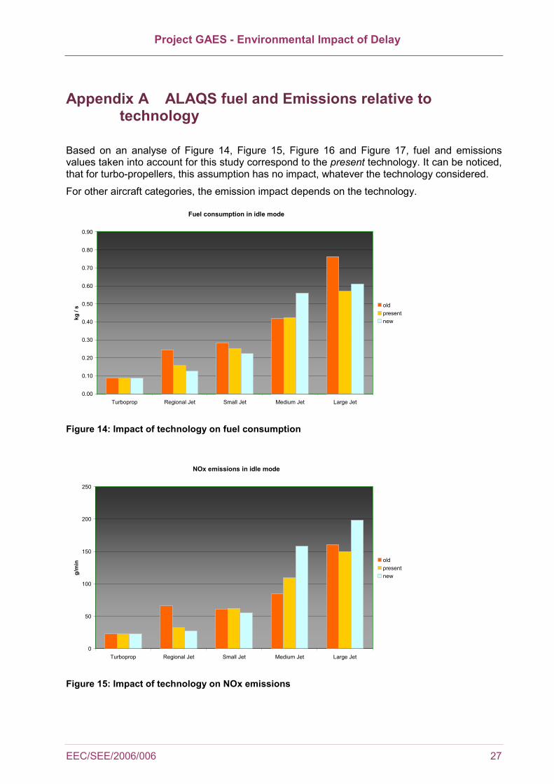
Based on an analyse of Figure 14, Figure 15, Figure 16 and Figure 17, fuel and emissions values taken into account for this study correspond to the present technology. It can be noticed, that for turbo-propellers, this assumption has no impact, whatever the technology considered.
For other aircraft categories, the emission impact depends on the technology.
Fuel consumption in idle mode
0.00
0.10
0.20
0.30
0.40
0.50
0.60
0.70
0.80
0.90
Turboprop Regional Jet Small Jet Medium Jet Large Jet
kg /
s oldpresentnew
Figure 14: Impact of technology on fuel consumption
NOx emissions in idle mode
0
50
100
150
200
250
Turboprop Regional Jet Small Jet Medium Jet Large Jet
g/m
in oldpresentnew
Figure 15: Impact of technology on NOx emissions

Project GAES - Environmental Impact of Delay
28 EEC/SEE/2006/006
HC emissions in idle mode
0
100
200
300
400
500
600
700
800
900
Turboprop Regional Jet Small Jet Medium Jet Large Jet
g/m
in old
presentnew
Figure 16: Impact of technology on HC emissions
CO emissions in idle mode
0
500
1000
1500
2000
2500
Turboprop Regional Jet Small Jet Medium Jet Large Jet
g/m
in old
presentnew
Figure 17: Impact of technology on CO emissions
Project GAES - Environmental Impact of Delay
EEC/SEE/2006/006 29
Appendix B Emission calculation NOx, HC and CO emission calculation is based on the Eurocontrol Modified Boeing Method 2 detailed in this appendix. This method combines atmospheric data, flight information and LTO emission indices in order to estimate NOx, HC and CO at altitude.
The aircraft/engines association relies on JP Airline-Fleets ([Ref 7.]) information: the most common engine for an aircraft type is assumed as representative. Exceptions are AT43 and AT72, for which actual engines are not available in the ICAO Engine Exhaust Emissions Data Bank ([Ref 6.]). An equivalent engine is thus attributed to AT43 and AT72.
B.1 Boeing method 2 – EUROCONTROL Modified This annex describes the EUROCONTROL modified Boeing Method 2 (EEC-BM2).
B.1.1 The original Boeing Method 2 (BM2) The International Civil Aviation Organisation (ICAO) has established standards and recommended practices (Annex 16 to the ICAO Conference, "Environmental Protection") for the testing of aircraft emissions on turbojet and turbofan engines. The world's jet engine manufacturers have been required to report to ICAO the results of required testing procedures, which pertain to aircraft emissions. ICAO regulations require reporting of emissions testing data on the following gaseous emissions: NOx, HC, CO and smoke. In addition to this, ICAO requires that information be reported on the rate of fuel flow at various phases of flight. Hence, ICAO maintains a database of this information, which is available for each of the phases of flight as ICAO defines them:
Operating Mode Fuel Throttle Setting (percent of maximum rated output)
Take-Off 100 %
Climb-Out 85 %
Approach 30 %
Taxi/ground idle 7 %
The Boeing Aircraft Company conducted an extensive study for NASA on emission inventories for scheduled civil aircraft worldwide (see Baugham et al., 1996). The Boeing 2 Method is an empirical procedure developed for this study, which computes in-flight aircraft emissions using, as a base, the measured fuel flow and the engine ICAO data sheets. Whereas the first Boeing method took into account ambient pressure, temperature and humidity, the second method was more complicated (and accurate). This new method allowed for ambient pressure, temperature and humidity as well as Mach number.
Project GAES - Environmental Impact of Delay
30 EEC/SEE/2006/006
Methodology The Boeing Method uses English units and not S.I. therefore the first step is to convert the Fuel Flow (Wf) from the ICAO data for a specific engine from kg/s to lbs/hr (multiply by 7936). The Emission Index (EI) values from ICAO are to be read as lbs/1000 lbs (same number as g/kg).
The ICAO fuel flow values are then to be modified by a correction for aircraft installation effects (Wf):
Take-Off 1.010
Climb-Out 1.013
Approach 1.020
Taxi/ground idle 1.100
STEP 1: Curve fitting the Data The Emission Indices (NOx, HC, CO) are to be plotted (log-log) against the corrected fuel flow (Wf).
STEP 2: Fuel Flow Factor
a) Calculate the values ∂amb (ambient pressure correction factor) and θamb (ambient temperature correction factor) where:
∂amb = 696.14
Pamb (Pamb = ambient (inlet) pressure) and
θamb = 15.288
15.273Tamb + (Tamb = ambient (inlet) temperature)
b) The fuel flow values are further modified by the ambient values:
Wff = 2M2.08.3
ambamb
f eW ××θ×∂
, where M is the Mach number.
c) Calculate the humidity correction factor H:
H = -19.0 × (ω - 0.0063), ω = specific humidity,
ω = vamb
vPP
P62198.0×Φ−
×Φ× .
where Φ is relative humidity and Pv = saturation vapour pressure in psia. For a correction to this formula, please see the EUROCONTROL corrected Boeing 2 Method below.
Pv = (0.014504) × 10β
and,
β =
+
−×16.273T
16.373190298.7amb
+ 3.00571 +
+
×16.273T
16.373log02808.5amb
10
+
−××
+−×− 16.373
16.273T 1344.117
amb
101103816.1 +
−××
+
−− 110101328.8 16.273T
16.373149149.33 amb

Project GAES - Environmental Impact of Delay
EEC/SEE/2006/006 31
STEP 3: Compute EI Calculate the emission indices of HC, CO and NOx:
EIHC = 02.1
3.3
amb
ambREIHC∂
× θ
EICO = 02.1amb
3.3ambREICO
∂θ×
EINOx = 3.3amb
02.1ambHeREINOx
θ∂××
Where the REIHC, REICO, and REINOx values are read off the graph (STEP 1) by substituting Wff for Wf.
STEP 4: Total Emission
Total (HC, CO, NOx) = ( )[ ]∑ −××××i
3ifi 10timeWEINOx EICO, EIHC,Engines of Number
i in lbs
Bibliography [Ref 6.] & [Ref 8.]
Project GAES - Environmental Impact of Delay
32 EEC/SEE/2006/006
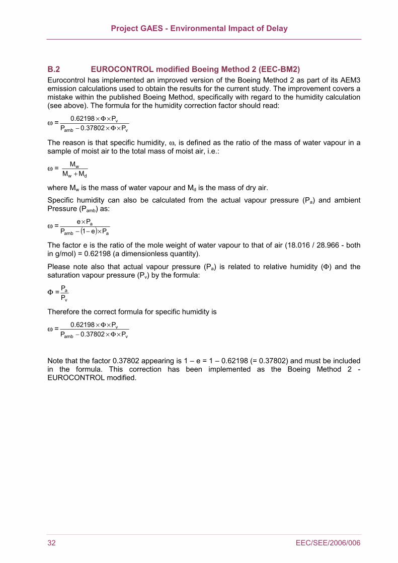
B.2 EUROCONTROL modified Boeing Method 2 (EEC-BM2) Eurocontrol has implemented an improved version of the Boeing Method 2 as part of its AEM3 emission calculations used to obtain the results for the current study. The improvement covers a mistake within the published Boeing Method, specifically with regard to the humidity calculation (see above). The formula for the humidity correction factor should read:
ω =vamb
vP37802.0P
P62198.0×Φ×−
×Φ×
The reason is that specific humidity, ω, is defined as the ratio of the mass of water vapour in a sample of moist air to the total mass of moist air, i.e.:
ω = dw
wMM
M+
where Mw is the mass of water vapour and Md is the mass of dry air.
Specific humidity can also be calculated from the actual vapour pressure (Pa) and ambient Pressure (Pamb) as:
ω = ( ) aamb
a
Pe1PPe
×−−×
The factor e is the ratio of the mole weight of water vapour to that of air (18.016 / 28.966 - both in g/mol) = 0.62198 (a dimensionless quantity).
Please note also that actual vapour pressure (Pa) is related to relative humidity (Φ) and the saturation vapour pressure (Pv) by the formula:
Φ =v
a
PP
Therefore the correct formula for specific humidity is
ω =vamb
vP37802.0P
P62198.0×Φ×−
×Φ×
Note that the factor 0.37802 appearing is 1 – e = 1 – 0.62198 (= 0.37802) and must be included in the formula. This correction has been implemented as the Boeing Method 2 - EUROCONTROL modified.

(This page intentionally blank)

For more information about the EEC Society, Environment and Economy Research Area please contact: Ted Elliff SEE Research Area Manager, EUROCONTROL Experimental Centre BP15, Centre de Bois des Bordes 91222 BRETIGNY SUR ORGE CEDEX France Tel: +33 1 69 88 73 36 Fax: +33 1 69 88 72 11 E-Mail: [email protected] or visit : http://www.eurocontrol.int/


