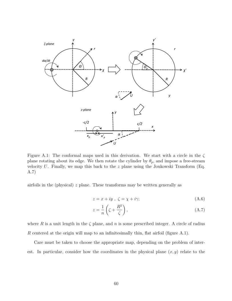
University of Calgary PRISM: University of Calgary's Digital Repository Graduate Studies The Vault: Electronic Theses and Dissertations 2015-02-02 The Aerodynamics of Rapid Area Change in Perching Manoeuvres Polet, Delyle Polet, D. (2015). The Aerodynamics of Rapid Area Change in Perching Manoeuvres (Unpublished master's thesis). University of Calgary, Calgary, AB. doi:10.11575/PRISM/28007 http://hdl.handle.net/11023/2050 master thesis University of Calgary graduate students retain copyright ownership and moral rights for their thesis. You may use this material in any way that is permitted by the Copyright Act or through licensing that has been assigned to the document. For uses that are not allowable under copyright legislation or licensing, you are required to seek permission. Downloaded from PRISM: https://prism.ucalgary.ca
Transcript
University of Calgary
PRISM: University of Calgary's Digital Repository
Graduate Studies The Vault: Electronic Theses and Dissertations
2015-02-02
The Aerodynamics of Rapid Area Change in Perching
Manoeuvres
Polet, Delyle
Polet, D. (2015). The Aerodynamics of Rapid Area Change in Perching Manoeuvres (Unpublished
master's thesis). University of Calgary, Calgary, AB. doi:10.11575/PRISM/28007
http://hdl.handle.net/11023/2050
master thesis
University of Calgary graduate students retain copyright ownership and moral rights for their
thesis. You may use this material in any way that is permitted by the Copyright Act or through
licensing that has been assigned to the document. For uses that are not allowable under
copyright legislation or licensing, you are required to seek permission.
Downloaded from PRISM: https://prism.ucalgary.ca
UNIVERSITY OF CALGARY
The Aerodynamics of Rapid Area Change in Perching Manoeuvres.
by
Delyle Thomas Polet
A THESIS
SUBMITTED TO THE FACULTY OF GRADUATE STUDIES
IN PARTIAL FULFILLMENT OF THE REQUIREMENTS FOR THE
DEGREE OF MASTER OF SCIENCE
DEPARTMENT OF MECHANICAL AND MANUFACTURING ENGINEERING
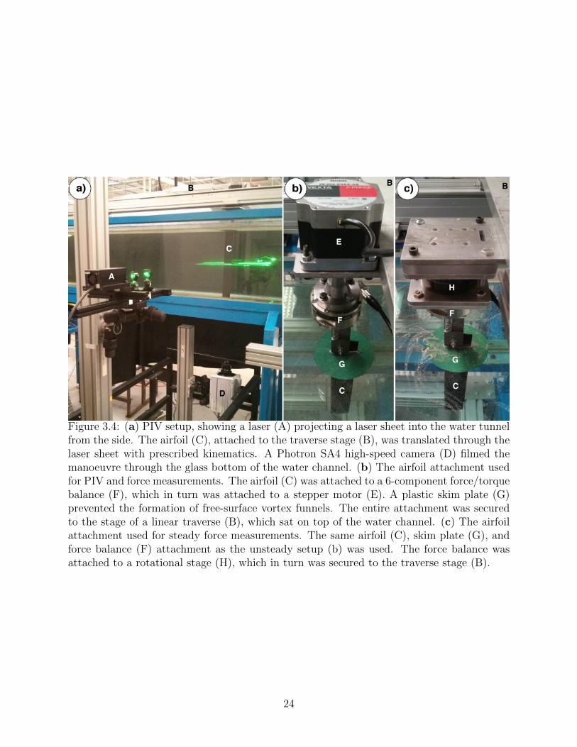
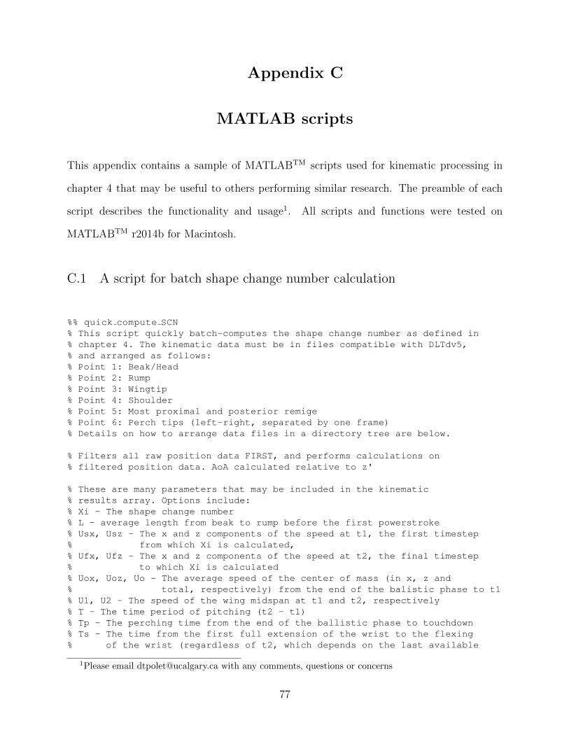
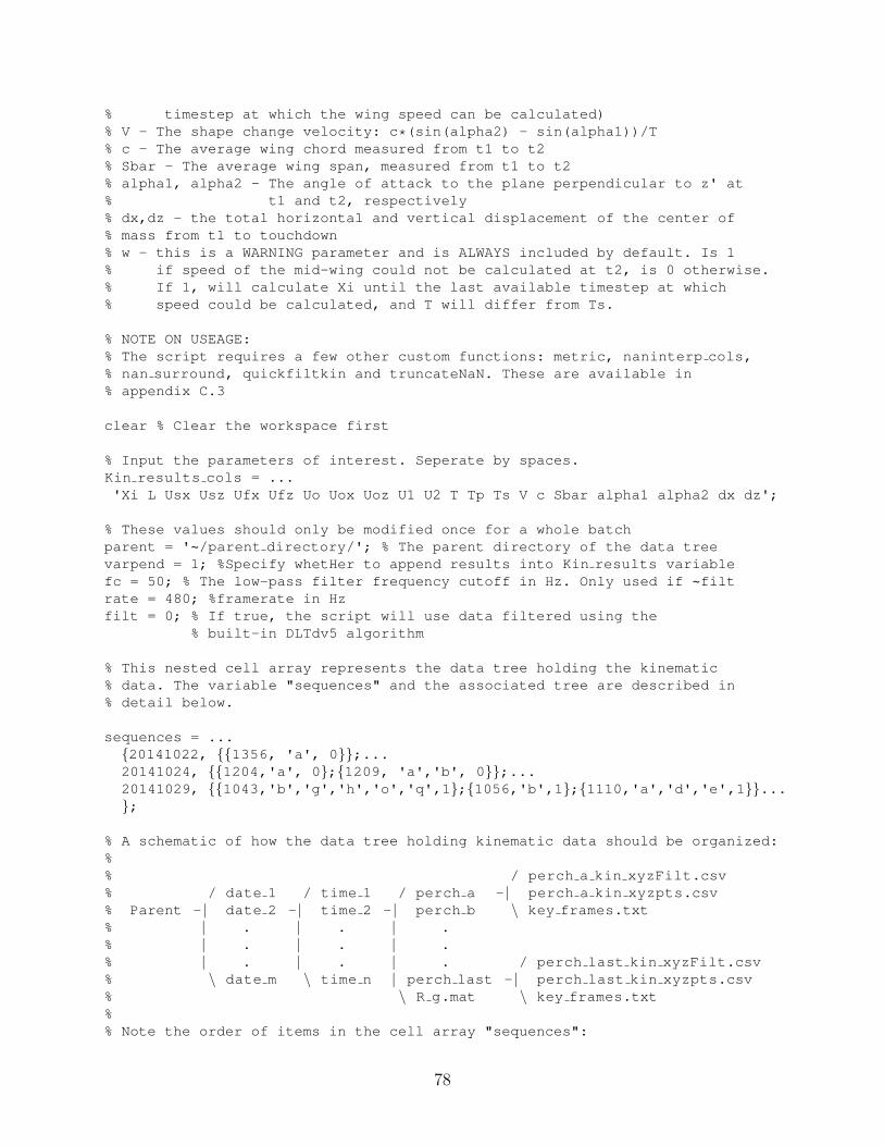
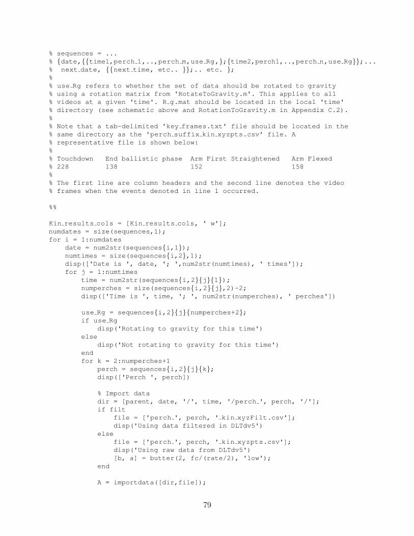
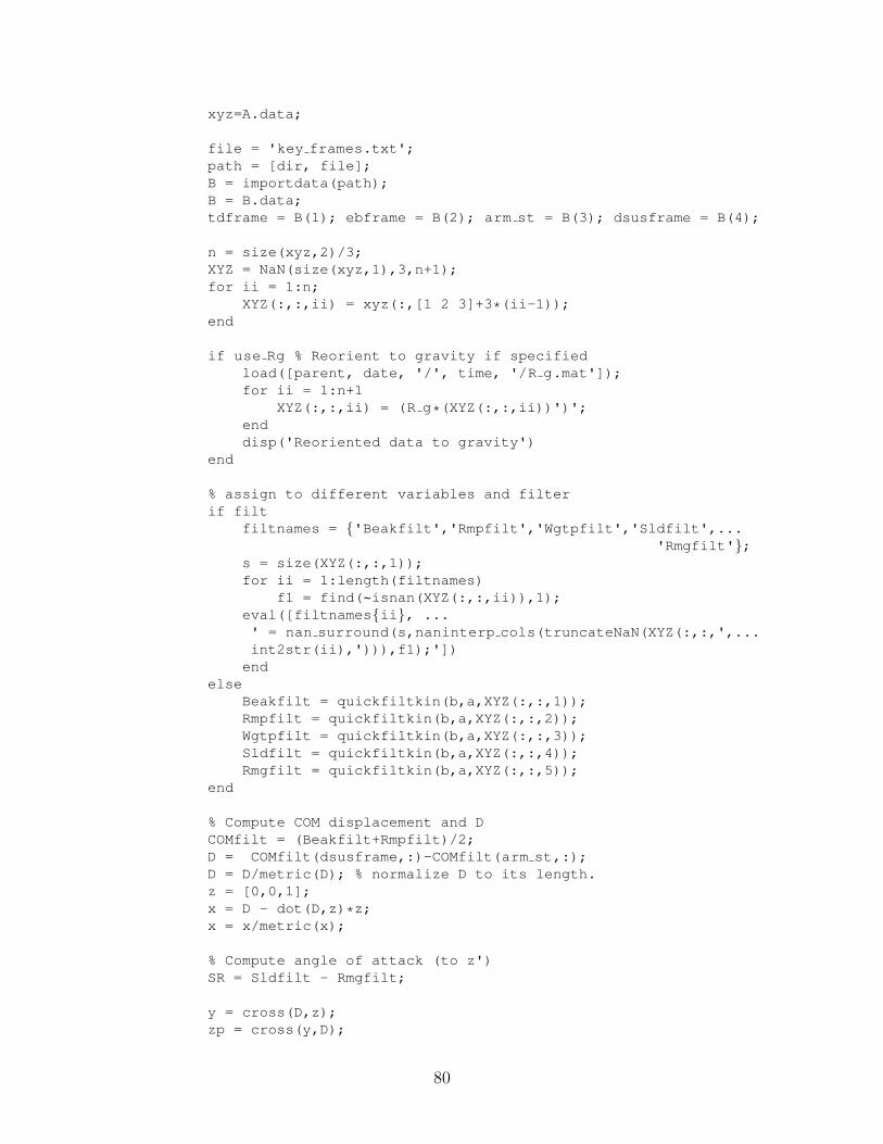
3.1 Estimates of uncertainty and signal-to-noise ratios (SNRdb, in decibels) for liftand drag. σf is the measured standard deviation of the peak force coefficientacross trials, and σt is the measured standard deviation of peak force time.Clmax and Cdmax are the peak average lift and drag coefficients, respectively. . 25
v
List of Figures and Illustrations
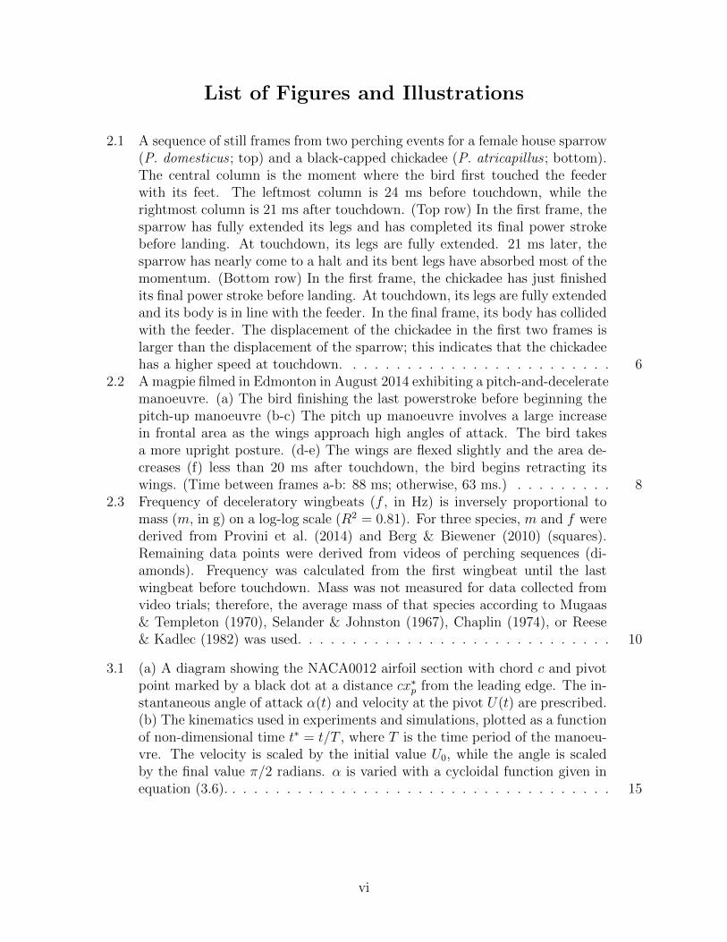
2.1 A sequence of still frames from two perching events for a female house sparrow(P. domesticus ; top) and a black-capped chickadee (P. atricapillus ; bottom).The central column is the moment where the bird first touched the feederwith its feet. The leftmost column is 24 ms before touchdown, while therightmost column is 21 ms after touchdown. (Top row) In the first frame, thesparrow has fully extended its legs and has completed its final power strokebefore landing. At touchdown, its legs are fully extended. 21 ms later, thesparrow has nearly come to a halt and its bent legs have absorbed most of themomentum. (Bottom row) In the first frame, the chickadee has just finishedits final power stroke before landing. At touchdown, its legs are fully extendedand its body is in line with the feeder. In the final frame, its body has collidedwith the feeder. The displacement of the chickadee in the first two frames islarger than the displacement of the sparrow; this indicates that the chickadeehas a higher speed at touchdown. . . . . . . . . . . . . . . . . . . . . . . . . 6
2.2 A magpie filmed in Edmonton in August 2014 exhibiting a pitch-and-deceleratemanoeuvre. (a) The bird finishing the last powerstroke before beginning thepitch-up manoeuvre (b-c) The pitch up manoeuvre involves a large increasein frontal area as the wings approach high angles of attack. The bird takesa more upright posture. (d-e) The wings are flexed slightly and the area de-creases (f) less than 20 ms after touchdown, the bird begins retracting itswings. (Time between frames a-b: 88 ms; otherwise, 63 ms.) . . . . . . . . . 8
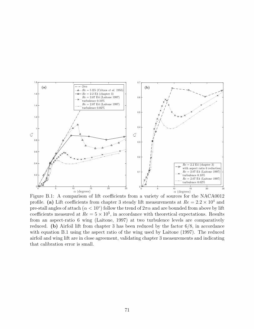
2.3 Frequency of deceleratory wingbeats (f , in Hz) is inversely proportional tomass (m, in g) on a log-log scale (R2 = 0.81). For three species, m and f werederived from Provini et al. (2014) and Berg & Biewener (2010) (squares).Remaining data points were derived from videos of perching sequences (di-amonds). Frequency was calculated from the first wingbeat until the lastwingbeat before touchdown. Mass was not measured for data collected fromvideo trials; therefore, the average mass of that species according to Mugaas& Templeton (1970), Selander & Johnston (1967), Chaplin (1974), or Reese& Kadlec (1982) was used. . . . . . . . . . . . . . . . . . . . . . . . . . . . . 10
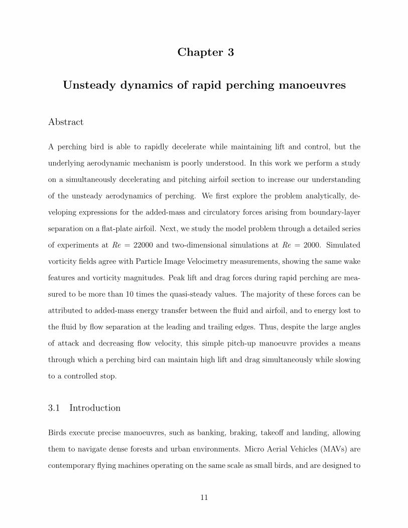
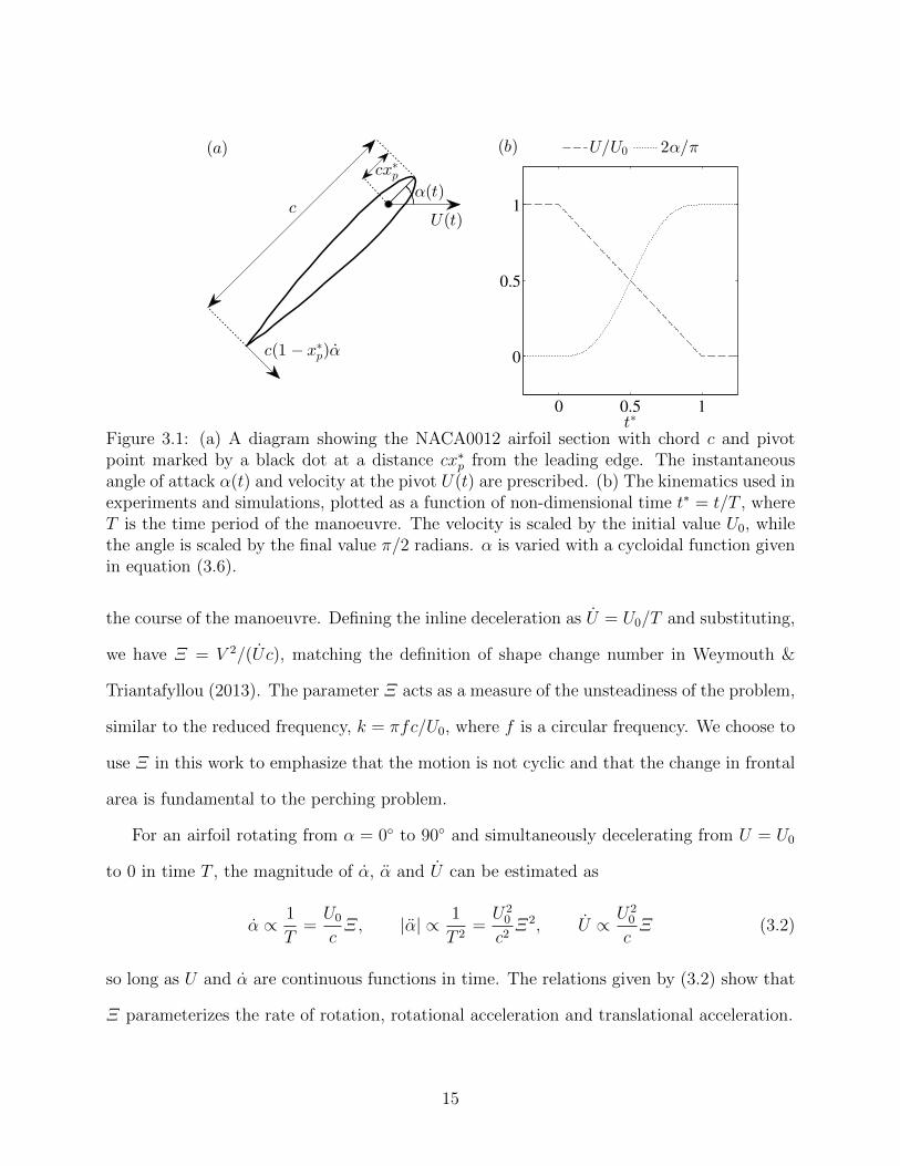
3.1 (a) A diagram showing the NACA0012 airfoil section with chord c and pivotpoint marked by a black dot at a distance cx∗p from the leading edge. The in-stantaneous angle of attack α(t) and velocity at the pivot U(t) are prescribed.(b) The kinematics used in experiments and simulations, plotted as a functionof non-dimensional time t∗ = t/T , where T is the time period of the manoeu-vre. The velocity is scaled by the initial value U0, while the angle is scaledby the final value π/2 radians. α is varied with a cycloidal function given inequation (3.6). . . . . . . . . . . . . . . . . . . . . . . . . . . . . . . . . . . . 15
vi
3.2 Predicted circulatory (equation (3.14), dashed lines) and added-mass (equa-tions (3.7) and (3.8), dotted lines) forces for the kinematic values given byequations (3.5-3.6). For lift, added-mass forces are most pronounced earlyin the manoeuvre but are quickly surpassed by circulatory forces. Peak cir-culatory drag dominates peak added-mass drag, however the parasitic thrustfrom the added-mass force overwhelms circulatory contributions late in themanoeuvre at high Ξ. As Ξ → 0, added-mass lift and drag approach zero. . 18
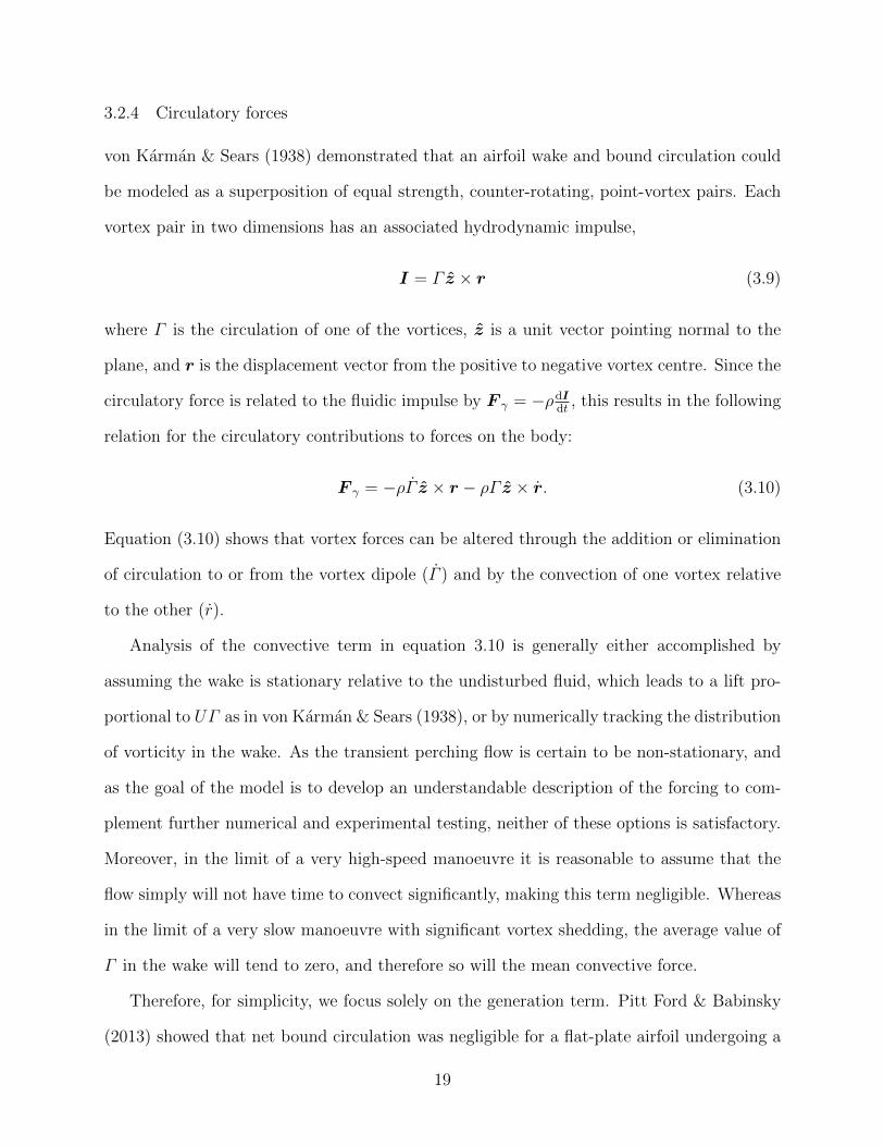
3.3 (Colour online) Sketch of the circulation production model. Velocity on thepressure side increases an amount equal to U⊥ while the separated fluid on thesuction side does not. This differential speed leads to a circulation per unitlength γ = ∆u‖ = U⊥ at the trailing edge. The negative vorticity in the wake,shown here as a blue line, increases in length at the trailing edge at a rateequal to the trailing-edge speed: ds
dt= Ute. This results in the total rate of
change of circulation Γ = dΓds
dsdt
= UteU⊥. The circulation of the LEV increasesby an equal and opposite amount in accordance with Kelvin’s Theorem. . . . 20
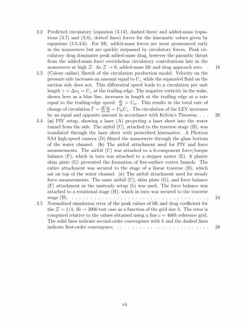
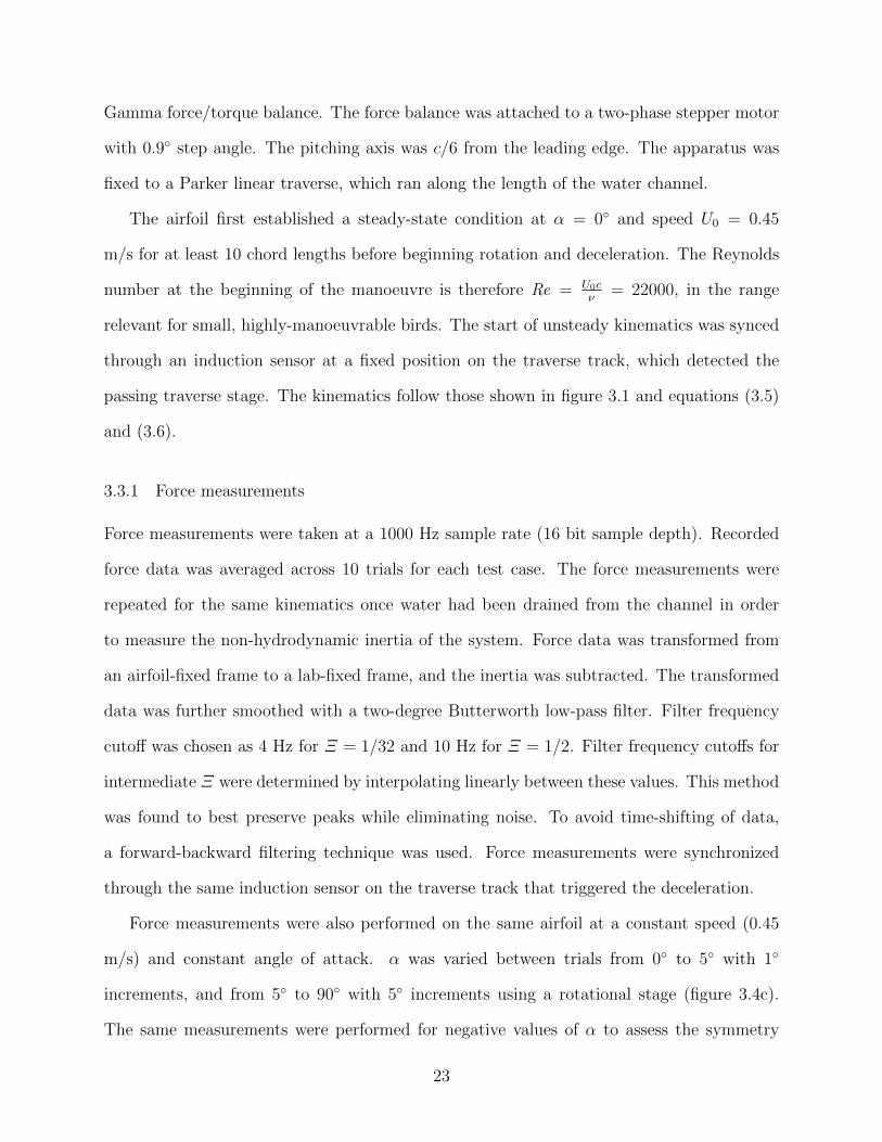
3.4 (a) PIV setup, showing a laser (A) projecting a laser sheet into the watertunnel from the side. The airfoil (C), attached to the traverse stage (B), wastranslated through the laser sheet with prescribed kinematics. A PhotronSA4 high-speed camera (D) filmed the manoeuvre through the glass bottomof the water channel. (b) The airfoil attachment used for PIV and forcemeasurements. The airfoil (C) was attached to a 6-component force/torquebalance (F), which in turn was attached to a stepper motor (E). A plasticskim plate (G) prevented the formation of free-surface vortex funnels. Theentire attachment was secured to the stage of a linear traverse (B), whichsat on top of the water channel. (c) The airfoil attachment used for steadyforce measurements. The same airfoil (C), skim plate (G), and force balance(F) attachment as the unsteady setup (b) was used. The force balance wasattached to a rotational stage (H), which in turn was secured to the traversestage (B). . . . . . . . . . . . . . . . . . . . . . . . . . . . . . . . . . . . . . 24
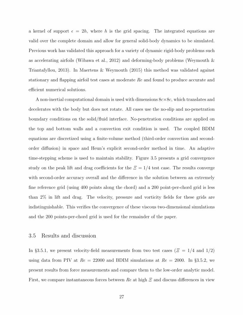
3.5 Normalized simulation error of the peak values of lift and drag coefficient forthe Ξ = 1/4, Re = 2000 test case as a function of the grid size h. The error iscomputed relative to the values obtained using a fine c = 400h reference grid.The solid lines indicate second-order convergence with h and the dashed linesindicate first-order convergence. . . . . . . . . . . . . . . . . . . . . . . . . . 28
vii
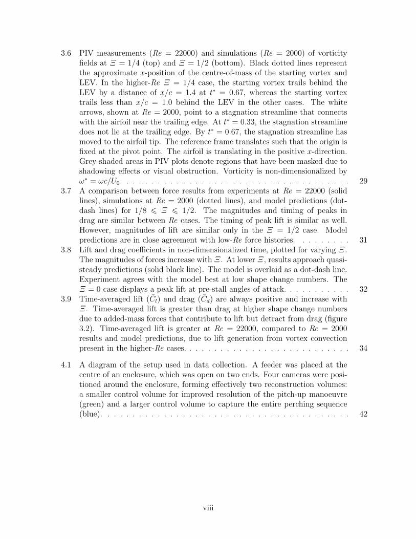
3.6 PIV measurements (Re = 22000) and simulations (Re = 2000) of vorticityfields at Ξ = 1/4 (top) and Ξ = 1/2 (bottom). Black dotted lines representthe approximate x-position of the centre-of-mass of the starting vortex andLEV. In the higher-Re Ξ = 1/4 case, the starting vortex trails behind theLEV by a distance of x/c = 1.4 at t∗ = 0.67, whereas the starting vortextrails less than x/c = 1.0 behind the LEV in the other cases. The whitearrows, shown at Re = 2000, point to a stagnation streamline that connectswith the airfoil near the trailing edge. At t∗ = 0.33, the stagnation streamlinedoes not lie at the trailing edge. By t∗ = 0.67, the stagnation streamline hasmoved to the airfoil tip. The reference frame translates such that the origin isfixed at the pivot point. The airfoil is translating in the positive x-direction.Grey-shaded areas in PIV plots denote regions that have been masked due toshadowing effects or visual obstruction. Vorticity is non-dimensionalized byω∗ = ωc/U0. . . . . . . . . . . . . . . . . . . . . . . . . . . . . . . . . . . . . 29
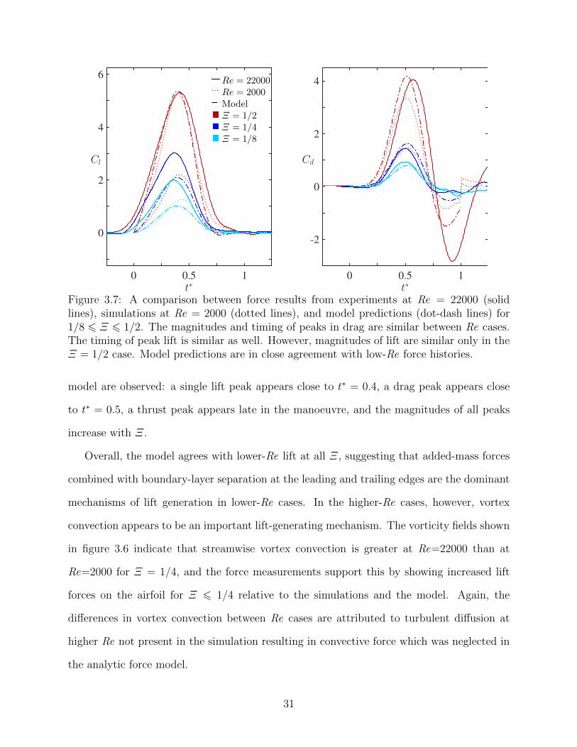
3.7 A comparison between force results from experiments at Re = 22000 (solidlines), simulations at Re = 2000 (dotted lines), and model predictions (dot-dash lines) for 1/8 6 Ξ 6 1/2. The magnitudes and timing of peaks indrag are similar between Re cases. The timing of peak lift is similar as well.However, magnitudes of lift are similar only in the Ξ = 1/2 case. Modelpredictions are in close agreement with low-Re force histories. . . . . . . . . 31
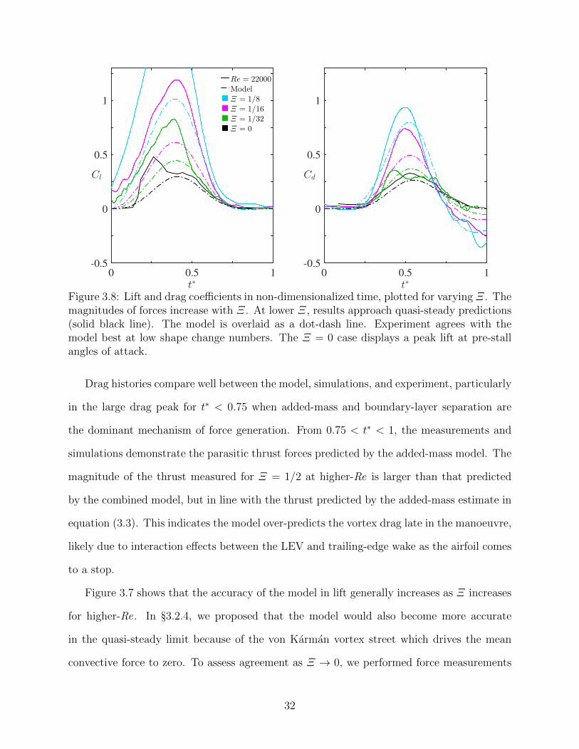
3.8 Lift and drag coefficients in non-dimensionalized time, plotted for varying Ξ.The magnitudes of forces increase with Ξ. At lower Ξ, results approach quasi-steady predictions (solid black line). The model is overlaid as a dot-dash line.Experiment agrees with the model best at low shape change numbers. TheΞ = 0 case displays a peak lift at pre-stall angles of attack. . . . . . . . . . . 32
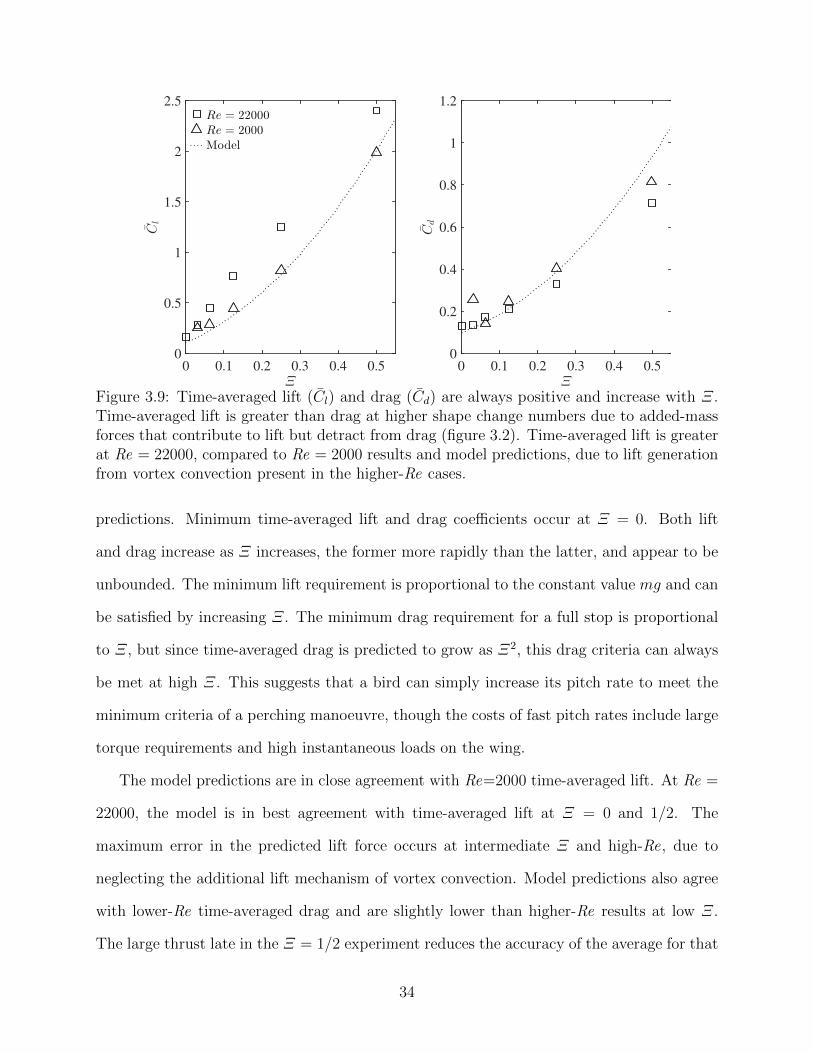
3.9 Time-averaged lift (Cl) and drag (Cd) are always positive and increase withΞ. Time-averaged lift is greater than drag at higher shape change numbersdue to added-mass forces that contribute to lift but detract from drag (figure3.2). Time-averaged lift is greater at Re = 22000, compared to Re = 2000results and model predictions, due to lift generation from vortex convectionpresent in the higher-Re cases. . . . . . . . . . . . . . . . . . . . . . . . . . . 34
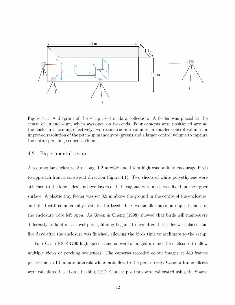
4.1 A diagram of the setup used in data collection. A feeder was placed at thecentre of an enclosure, which was open on two ends. Four cameras were posi-tioned around the enclosure, forming effectively two reconstruction volumes:a smaller control volume for improved resolution of the pitch-up manoeuvre(green) and a larger control volume to capture the entire perching sequence(blue). . . . . . . . . . . . . . . . . . . . . . . . . . . . . . . . . . . . . . . . 42
viii
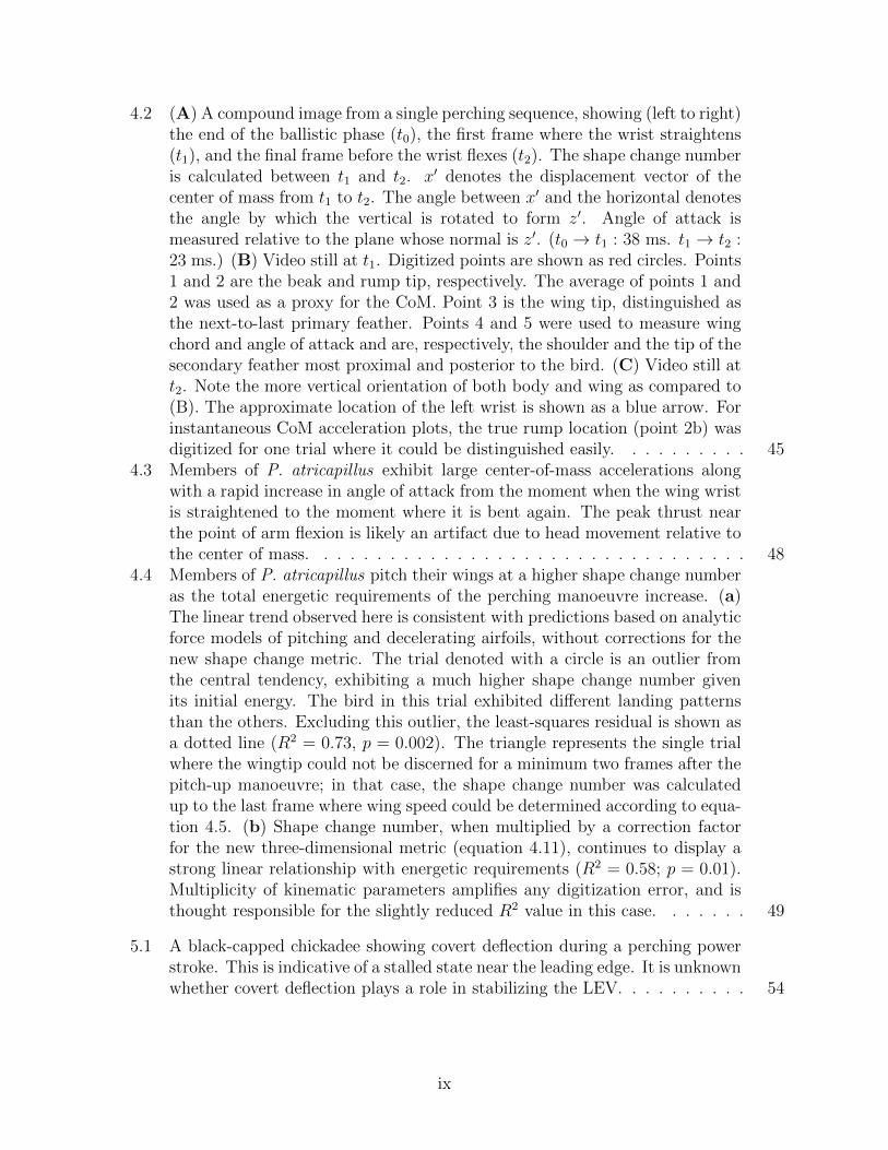
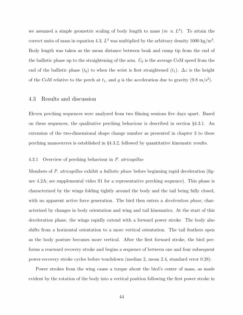
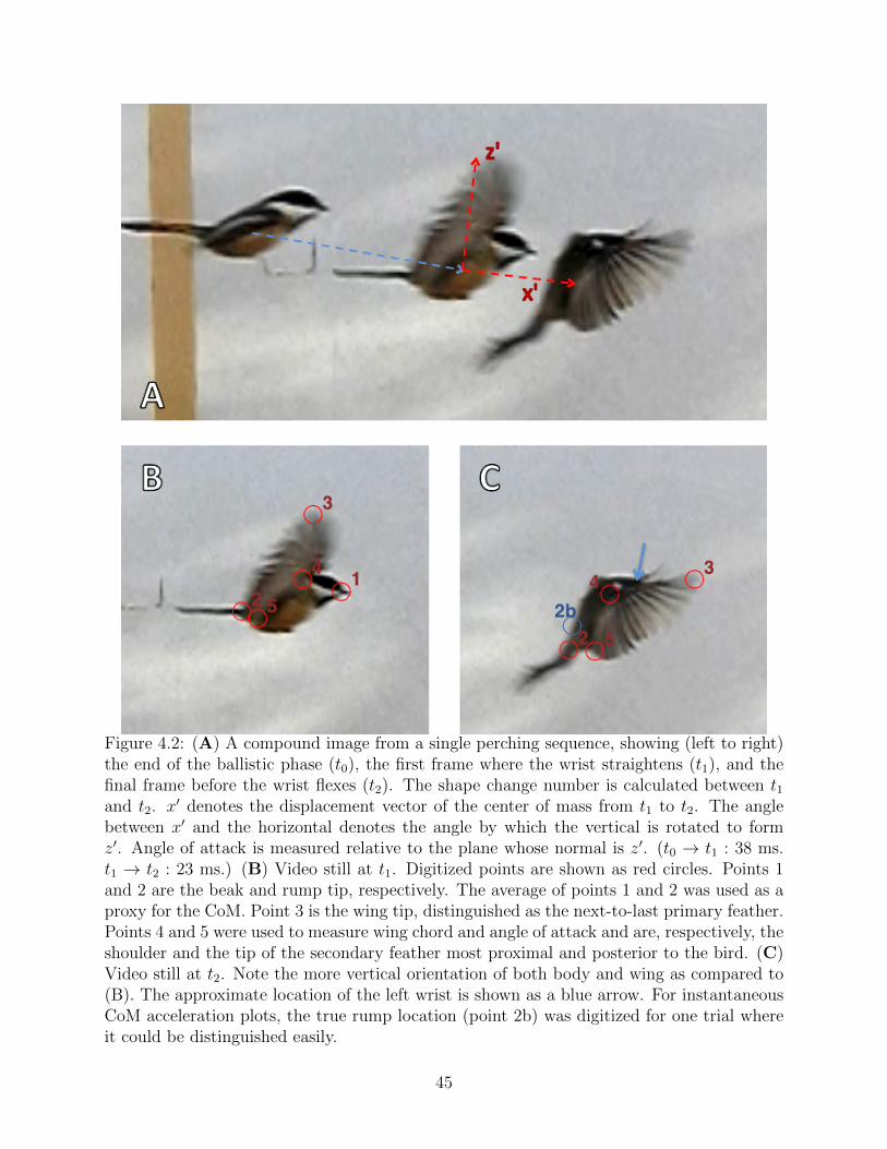
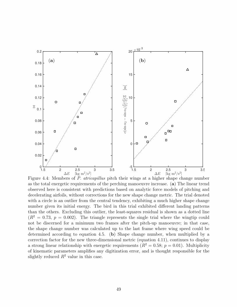
4.2 (A) A compound image from a single perching sequence, showing (left to right)the end of the ballistic phase (t0), the first frame where the wrist straightens(t1), and the final frame before the wrist flexes (t2). The shape change numberis calculated between t1 and t2. x′ denotes the displacement vector of thecenter of mass from t1 to t2. The angle between x′ and the horizontal denotesthe angle by which the vertical is rotated to form z′. Angle of attack ismeasured relative to the plane whose normal is z′. (t0 → t1 : 38 ms. t1 → t2 :23 ms.) (B) Video still at t1. Digitized points are shown as red circles. Points1 and 2 are the beak and rump tip, respectively. The average of points 1 and2 was used as a proxy for the CoM. Point 3 is the wing tip, distinguished asthe next-to-last primary feather. Points 4 and 5 were used to measure wingchord and angle of attack and are, respectively, the shoulder and the tip of thesecondary feather most proximal and posterior to the bird. (C) Video still att2. Note the more vertical orientation of both body and wing as compared to(B). The approximate location of the left wrist is shown as a blue arrow. Forinstantaneous CoM acceleration plots, the true rump location (point 2b) wasdigitized for one trial where it could be distinguished easily. . . . . . . . . . 45
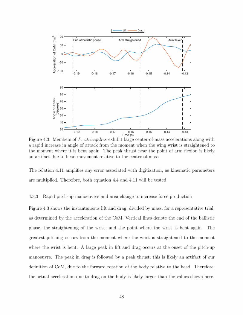
4.3 Members of P. atricapillus exhibit large center-of-mass accelerations alongwith a rapid increase in angle of attack from the moment when the wing wristis straightened to the moment where it is bent again. The peak thrust nearthe point of arm flexion is likely an artifact due to head movement relative tothe center of mass. . . . . . . . . . . . . . . . . . . . . . . . . . . . . . . . . 48
4.4 Members of P. atricapillus pitch their wings at a higher shape change numberas the total energetic requirements of the perching manoeuvre increase. (a)The linear trend observed here is consistent with predictions based on analyticforce models of pitching and decelerating airfoils, without corrections for thenew shape change metric. The trial denoted with a circle is an outlier fromthe central tendency, exhibiting a much higher shape change number givenits initial energy. The bird in this trial exhibited different landing patternsthan the others. Excluding this outlier, the least-squares residual is shown asa dotted line (R2 = 0.73, p = 0.002). The triangle represents the single trialwhere the wingtip could not be discerned for a minimum two frames after thepitch-up manoeuvre; in that case, the shape change number was calculatedup to the last frame where wing speed could be determined according to equa-tion 4.5. (b) Shape change number, when multiplied by a correction factorfor the new three-dimensional metric (equation 4.11), continues to display astrong linear relationship with energetic requirements (R2 = 0.58; p = 0.01).Multiplicity of kinematic parameters amplifies any digitization error, and isthought responsible for the slightly reduced R2 value in this case. . . . . . . 49
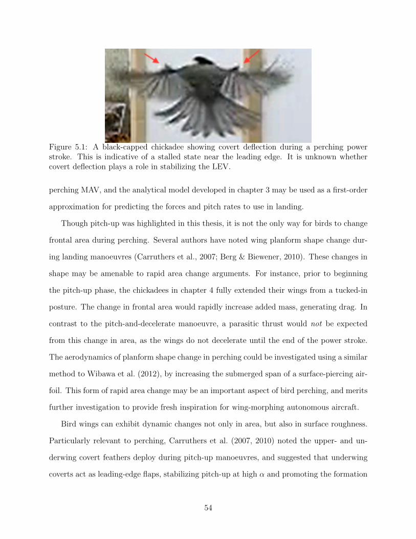
5.1 A black-capped chickadee showing covert deflection during a perching powerstroke. This is indicative of a stalled state near the leading edge. It is unknownwhether covert deflection plays a role in stabilizing the LEV. . . . . . . . . . 54
ix
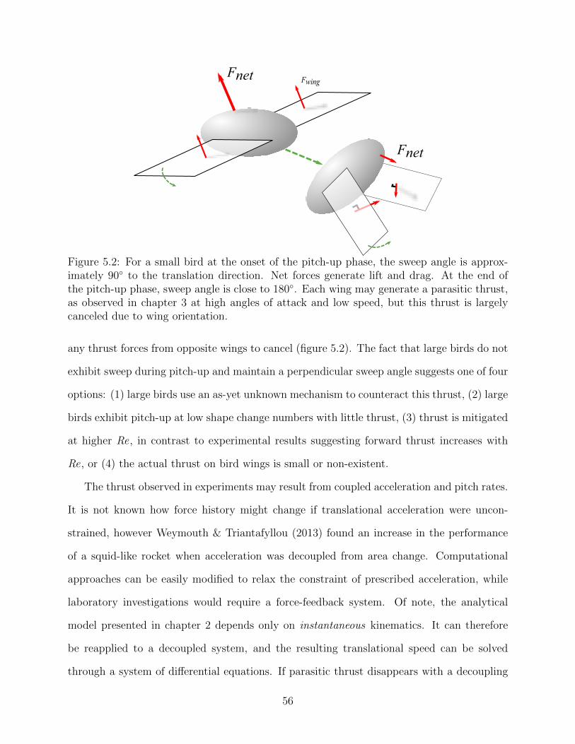
5.2 For a small bird at the onset of the pitch-up phase, the sweep angle is approx-imately 90 to the translation direction. Net forces generate lift and drag. Atthe end of the pitch-up phase, sweep angle is close to 180. Each wing maygenerate a parasitic thrust, as observed in chapter 3 at high angles of attackand low speed, but this thrust is largely canceled due to wing orientation. . . 56
A.1 The conformal maps used in this derivation. We start with a circle in the ζplane rotating about its edge. We then rotate the cylinder by θp, and imposea free-stream velocity U . Finally, we map this back to the z plane using theJoukowski Transform (Eq. A.7) . . . . . . . . . . . . . . . . . . . . . . . . . 60
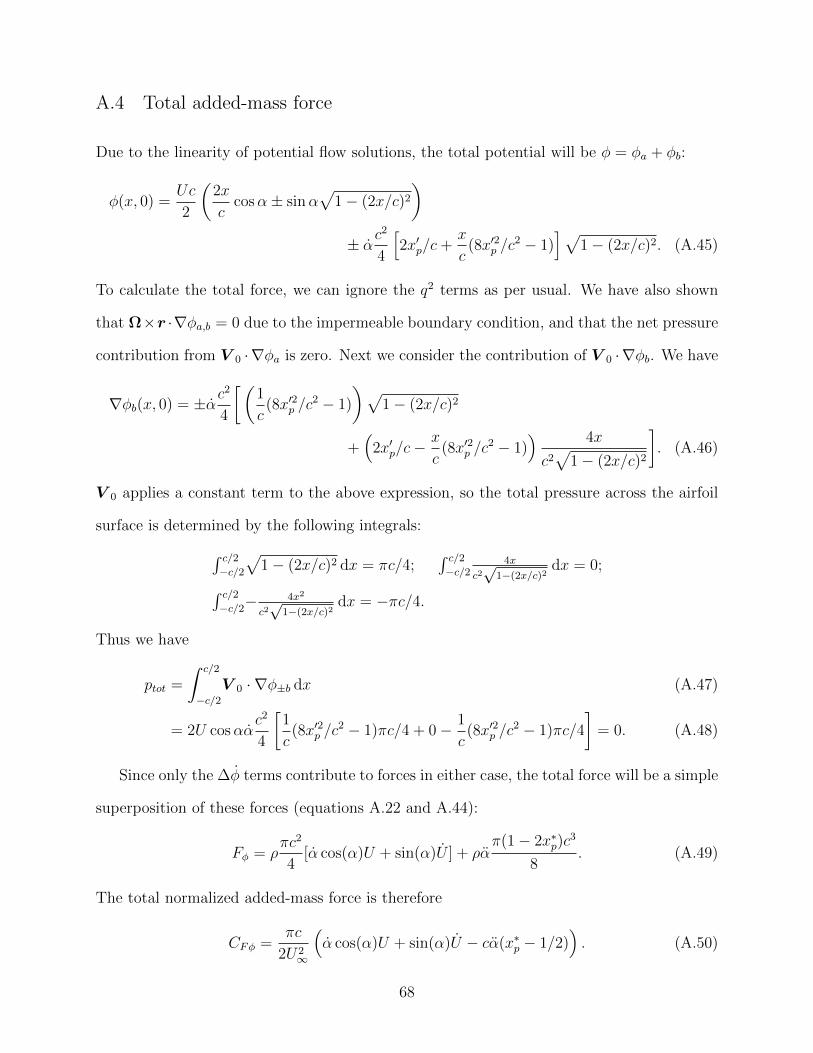
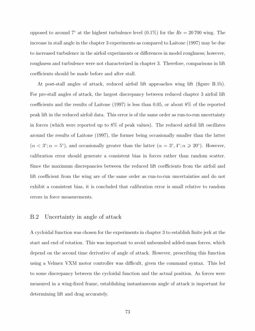
B.1 A comparison of lift coefficients from a variety of sources for the NACA0012profile. (a) Lift coefficients from chapter 3 steady lift measurements at Re =2.2 × 10⁴ and pre-stall angles of attach (α < 10) follow the trend of 2παand are bounded from above by lift coefficients measured at Re = 5 × 10⁵,in accordance with theoretical expectations. Results from an aspect-ratio 6wing (Laitone, 1997) at two turbulence levels are comparatively reduced. (b)Airfoil lift from chapter 3 has been reduced by the factor 6/8, in accordancewith equation B.1 using the aspect ratio of the wing used by Laitone (1997).The reduced airfoil and wing lift are in close agreement, validating chapter 3measurements and indicating that calibration error is small. . . . . . . . . . 71
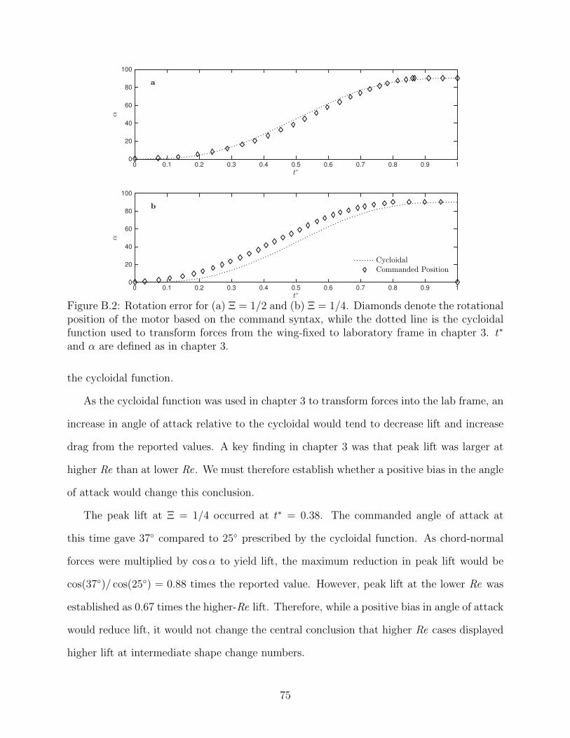
B.2 Rotation error for (a) Ξ = 1/2 and (b) Ξ = 1/4. Diamonds denote therotational position of the motor based on the command syntax, while thedotted line is the cycloidal function used to transform forces from the wing-fixed to laboratory frame in chapter 3. t∗ and α are defined as in chapter3. . . . . . . . . . . . . . . . . . . . . . . . . . . . . . . . . . . . . . . . . . . 75
x
List of Symbols, Abbreviations and Nomenclature
Abbreviation DefinitionBDIM Boundary Data Immersion MethodCoM Center of MassLED Light-Emitting DiodeLEV Leading-Edge VortexMAV Micro Aerial VehiclePIV Particle Image VelocimetrySNRdB Signal to Noise Ratio in decibels
Symbol Definitiona AccelerationA Wing planform areac Airfoil or wing chord lengthCl, Cd Coefficient of lift and drag, respectivelyCl, Cd Time-averaged coefficient of lift and drag, respectivelyClmax, Cdmax Peak average coefficient of lift and drag, respectivelyCFφ Chord-normal added-mass force coefficientCFφ Chord-normal circulatory force coefficientCF Net chord-normal force coefficientCpL, CpD Pressure force lift and drag coefficients, respectivelyd Translational distanceD Dragf FrequencyF Force magnitudeFAM Added-mass forceF γ Circulatory forceg Acceleration due to gravityh Computational grid spacingi (As a subscript) frame numberI Hydrodynamic impulsek Reduced frequencyL Body lengthm Massma Added massn Sample sizen Surface unit normal vectorq Fluid speedr Radial distance (in polar coordinates)Re Reynolds numbers Distance along trailing-edge wakeS Wingspan
xi
t Dimensional timet0 Time at the end of the ballistic phase during perchingt1 Time when wrist is first fully extended during perchingt2 Time when wrist is first flexed after full extension
during perchingt∗ Time, normalized by TT Time periodu Velocityu‖, u⊥ Flow speed parallel and perpendicular to airfoil chord,
respectivelyU Instantaneous translational speedU0 Initial or reference speedU∞ Far-field flow speedU⊥ Trailing edge speed perpendicular to the airfoil chordUte Total trailing edge speedvb Body velocityV Average speed of frontal area increaseV 0 Translational velocity of a body in fluidx, y, z Unit vector in x, y and z directionsx Displacement relative to the originx∗p Pivot distance from leading edge, normalized by cα Angle of attackα1, α2 Angle of attack at t1 and t2, respectivelyγ Circulation per unit lengthΓ Circulation∆E Total change in kinetic and potential energy during
perching∆t Time increment∆U Characteristic velocity change during pitch-up∆z Height of a bird’s CoM relative to perch at the onset of
perchingη∗p Pivot distance from trailing edge, normalized by cλ Wavelengthν Dynamic viscosityΞ Shape change numberρ Mass per unit volumeσ Standard deviationσf , σt Measured standard deviations of peak force magnitude
and time, respectivelyφ Velocity potentialΩ Rotational velocity of a body in fluid
xii
Chapter 1
Introduction
Birds are an amazingly diverse clade of vertebrates, consisting of about 10 000 species (Camp-
bell et al., 2008). As most of these species can fly, they represent a trove of inspiration for
flying machines. Flight in birds has been evolving for more than 140 million years by some
estimates (Zhou, 2004), making them incredibly experienced fliers. Man’s experience with
flying machines pales in comparison to nature’s: the earliest examples of human-designed
aircraft are kites (Deng, 2011) and hovering rotary tops (Leishman, 2006) from fifth-century
B.C. in China. More recently, there has been great interest in developing small flying vehi-
cles for use in reconnaissance, search and rescue, and surveying operations. Dubbed Micro
Aerial Vehicles (MAVs), the goal is to develop aircraft that have a mass less than 30 g, a
wingspan of about 8 cm, and speeds up to 65 km/h (Mueller & DeLaurier, 2001). These
machines should also be manoeuvrable, able to navigate narrow corridors and regions hard
to reach by humans.
Small birds fill these criteria well, are highly manoeuvrable flyers, and could serve as
inspiration for the next generation of man-made flying machines. Birds must solve some of
the same problems as MAVs (e.g. flight at small scales, navigation and obstacle avoidance)
but must also contend with other problems (e.g. digestion and reproduction). Rather than
blindly copying natural behaviour in artificial machines, we can first attempt to uncover the
physical mechanisms used in the natural system. This allows us to not only understand how
birds solve the problems we are interested in, but also to improve on these designs for our
own specific needs.
Birds are able to perform an array of unsteady manoeuvres, allowing them to navigate
cluttered airspaces. Mimicking these abilities would allow MAVs to complete the most de-
1
manding remote sensing tasks effectively and efficiently. Perching is one such manoeuvre,
characterized by a controlled deceleration to land on a small platform. This thesis investi-
gates the perching behaviour of birds and the underlying physics. Though perching is the
central focus, many of the strategies used could be reapplied to other unsteady manoeuvres,
such as braking or banking.
A multi-disciplinary approach is taken to explore the perching problem. Chapter 2 is
an overview of perching strategies in birds, highlighting the complexity of the problem and
some of the considerations biologists and engineers must take in interpreting behaviour. The
scope is then narrowed to the use of rapid area change in perching birds; in particular, how
a pitch-up manoeuvre alters frontal area and so drastically modifies forces.
Chapter 3 explores the physics of a pitch-and-decelerate manoeuvre in an airfoil as a
simple abstraction of a perching bird. Simple analytic models are developed and incorporated
from prior work, and are tested on simulations and experiments in a water tunnel. The model
and observed forces help explain the advantages and disadvantages of such manoeuvres
for perching birds. Chapter 4 returns to the actual organisms, showing how a small bird
(the black-capped chickadee; Poecile atricapillus, Linnaeus 1766) uses rapid area change
through a pitch-up manoeuvre to quickly dissipate energy and land safely. Some of the
behaviours observed in these birds are explained through the physics developed in chapter
3. Chapter 5 is a synthesis of the previous chapters, reviewing how simple analytical models
explain forces observed in a perching airfoil, how this in turn explains behaviour in the
black-capped chickadee, and the implications for MAV design. Finally, interesting avenues
of future research are highlighted.
Chapters 3 and 4 are written in the format of journal articles. The author of this thesis
is first author on both these works. Chapter 3 has been accepted for publication in the
Journal of Fluid Mechanics (2015, in press), under the title Unsteady Dynamics of Rapid
Perching Manoeuvres. The co-authors, Dr. David Rival and Dr. Gabriel Weymouth, advised
2
the primary author in data collection, modelling and analysis and edited the manuscript
before submission. Dr. Weymouth performed the computational experiments. Chapter
4 is a preliminary manuscript intended for publication in the journal Bioinspiration and
Biomimetics under the title Rapid area change from pitch-up manoeuvres in a small perching
bird. Dr. David Rival is co-author on this work. Three appendices are also included in this
thesis. Appendix A shows a derivation of the added-mass force on a pitching and accelerating
airfoil. Appendix B discusses chapter 3 experimental error in greater detail. Appendix C
provides MATLABTM scripts for use in kinematic analyses of perching birds.
3
Chapter 2
Overview of perching strategies in birds
Perching is an unsteady manoeuvre that has attracted the attention of biologists and en-
gineers alike. It is complex, as the bird must carefully balance competing costs: too much
speed at landing, and the bird risks crashing into the perch; too little speed requires extra
energy to stay airborne. The rate of deceleration is equally important; slow deceleration re-
quires long periods of sustained lift, but rapid deceleration hinders control and puts greater
stresses on the bird. Optimal kinematics for a controlled, efficient and safe landing are not
obvious, and are likely to change depending on circumstance, species and size.
A perching bird must coordinate visual cues, proprioception, muscle activation and care-
ful kinematic adjustments to stay airborne; it must decelerate safely but efficiently, respond
to changes in fluid speed, and land in a controlled manner on a small landing platform. The
numerous demands on the bird yield many factors that contribute to variation in perching
behaviour. Presently, these factors are broadly categorized as physiological, cognitive and
aerodynamic. The first two categories are presented generally for completeness, while the
latter is the central focus of this thesis.
Physiological factors play into a bird’s ability to perch effectively. A bird needs to be
able to not only land, but cruise, takeoff, and perform other biological functions besides
flight. These biological needs sometimes compete; thus the design of a bird is a compromise
weighted by its ecological specialty. Birds that perform more unsteady manoeuvres tend to
have relatively thick wing skeletal elements, and a relatively large distribution of forearm
muscle (Dial, 1992b). Birds lacking these features have more difficulty performing unsteady
manoeuvres such as perching. Power demands on the main downstroke muscle in rock pigeons
(Columba livia, Gmelin 1789) are higher during landing flight than takeoff and cruising flight
4
(Biewener et al., 1998), and members of the same species with forearm muscles disabled are
able to maintain cruising flight but not landing (Dial, 1992b). Landing also strains the
skeletal elements of legs. Starlings (Sturnus vulgaris, Linnaeus 1758) sustain an average of
1.8 times their body weight in the legs during landing (Bonser & Rayner, 1996), while rock
pigeons sustain up to eight times their body weight in landing (Green & Cheng, 1998).
Cognitive and behavioural factors can influence a bird’s perching behaviour. Green &
Cheng (1998) found that rock pigeons would approach a novel perch more slowly than
a familiar perch. Tobalske et al. (2004) found hummingbirds frightened into a take-off
generated larger forces compared to individuals who took off voluntarily to feed. Provini et al.
(2014) suggested emotional state may also affect landing behaviour in a similar way. Foraging
strategies can also influence the observed kinematics in birds. Black-capped chickadees
(Poecile atricapillus, Linnaeus 1766) in Calgary, Alberta were observed to land at a feeder,
grab a single seed and dart off quickly (n=5). In contrast, house sparrows (Passer domesticus,
Linnaeus 1758) fed at the same feeder for minutes at a time (n=10). Accordingly, speed at
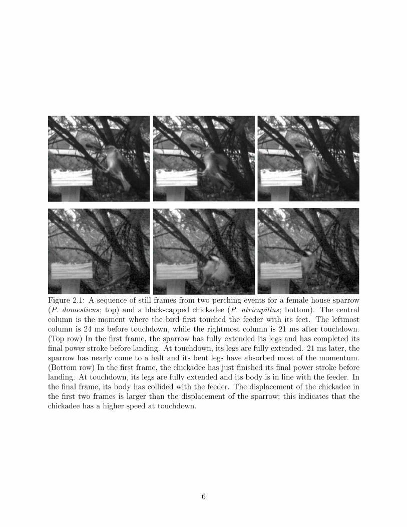
touchdown was larger in chickadees compared to sparrows (figure 2.1), consistent with the
preference of chickadees to spend less time in the open.
Though all these factors influence perching in birds, it would be intractable to consider
them all in detail in the present work. Instead, this thesis focuses on the aerodynamics
of perching in small birds: how and to what degree the observed kinematics in birds can
be explained through aerodynamic mechanisms. Once we understand the aerodynamics of
perching, we can distinguish which designs in nature are best for force production under a
given set of circumstances, and better replicate and improve on these designs in biomimetic
flying machines.
Aerodynamic mechanisms account for the majority of energy dissipation during perch-
ing. Provini et al. (2014) observed 32 times more energy dissipated aerodynamically than
through the legs in a perching diamond dove (Geopelia cuneata, Latham 1801). The pre-
5
Figure 2.1: A sequence of still frames from two perching events for a female house sparrow(P. domesticus ; top) and a black-capped chickadee (P. atricapillus ; bottom). The centralcolumn is the moment where the bird first touched the feeder with its feet. The leftmostcolumn is 24 ms before touchdown, while the rightmost column is 21 ms after touchdown.(Top row) In the first frame, the sparrow has fully extended its legs and has completed itsfinal power stroke before landing. At touchdown, its legs are fully extended. 21 ms later, thesparrow has nearly come to a halt and its bent legs have absorbed most of the momentum.(Bottom row) In the first frame, the chickadee has just finished its final power stroke beforelanding. At touchdown, its legs are fully extended and its body is in line with the feeder. Inthe final frame, its body has collided with the feeder. The displacement of the chickadee inthe first two frames is larger than the displacement of the sparrow; this indicates that thechickadee has a higher speed at touchdown.
6
cise kinematics generating aerodynamic forces vary between species and depend on external
factors (e.g. distance from the perch or ambient windspeed (Carruthers et al., 2007)). How-
ever, some patterns emerge. Birds reorient their bodies from a horizontal to vertical posture
during landing (Carruthers et al., 2007; Berg & Biewener, 2010; Provini et al., 2014), and
exhibit higher angles of attack and stroke amplitude when landing or flying more slowly
(Dial, 1992a; Tobalske & Dial, 1996; Tobalske et al., 2003; Carruthers et al., 2007; Berg &
Biewener, 2010).
Several authors have also noted a change in wing shape during landing (Carruthers
et al., 2007; Berg & Biewener, 2010). Adjustments of wing shape and a consistent pattern
of more upright posture suggest that modification of frontal area generates forces during
perching. Studies on rapid area change have shown that large forces can be explained
through a combination of boundary-layer vorticity effects and added-mass manipulation
(Wibawa et al., 2012; Weymouth & Triantafyllou, 2012, 2013). An obvious yet overlooked
method of changing frontal area during flight is to simply pitch control surfaces to larger
angles of attack.
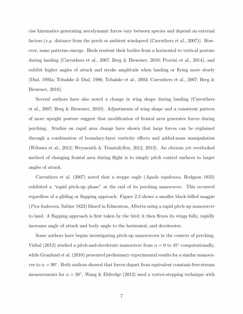
Carruthers et al. (2007) noted that a steppe eagle (Aquila nipalensis, Hodgson 1833)
exhibited a “rapid pitch-up phase” at the end of its perching manoeuvre. This occurred
regardless of a gliding or flapping approach. Figure 2.2 shows a smaller black-billed magpie
(Pica hudsonia, Sabine 1823) filmed in Edmonton, Alberta using a rapid pitch-up manoeuvre
to land. A flapping approach is first taken by the bird; it then flexes its wings fully, rapidly
increases angle of attack and body angle to the horizontal, and decelerates.
Some authors have begun investigating pitch-up manoeuvres in the context of perching.
Visbal (2012) studied a pitch-and-decelerate manoeuvre from α = 0 to 45 computationally,
while Granlund et al. (2010) presented preliminary experimental results for a similar manoeu-
vre to α = 90. Both authors showed that forces depart from equivalent constant-free-stream
measurements for α > 30. Wang & Eldredge (2012) used a vortex-stepping technique with
7
Figure 2.2: A magpie filmed in Edmonton in August 2014 exhibiting a pitch-and-deceleratemanoeuvre. (a) The bird finishing the last powerstroke before beginning the pitch-up ma-noeuvre (b-c) The pitch up manoeuvre involves a large increase in frontal area as the wingsapproach high angles of attack. The bird takes a more upright posture. (d-e) The wings areflexed slightly and the area decreases (f) less than 20 ms after touchdown, the bird beginsretracting its wings. (Time between frames a-b: 88 ms; otherwise, 63 ms.)
only two point vortices to predict forces in a perching manoeuvre. This technique involved
far fewer degrees of freedom than typical computational methods, and demonstrated decent
agreement with experiment. However, a time-stepping procedure, even with a small number
of vortices, does not directly connect kinematics to observed forces. The lack of physical
understanding of the mechanisms of force generation in perching manoeuvres inhibits their
application to MAVs and limits understanding biological systems.
While Berg & Biewener (2010) measured average angle of attack in time for individual
deceleratory strokes, no existing studies have quantified the rate of continuous pitch-up in
a perching bird; therefore, appropriate pitch rates to test experimentally are not known.
The tests run by Visbal (2012) and Granlund et al. (2010) were performed at Re < 50 000,
while the magpie and eagle that were observed performing pitch-and-decelerate manoeuvres
operate at Re > 100 000. The assumption that rapid pitch-up is appropriate for perching
aircraft as small as MAVs is as yet without basis in the animal kingdom.
To explore possible differences in perching strategies across size ranges, four bird species
8
were filmed in perching manoeuvres in Calgary and Edmonton, Alberta between July 2013
and September 2014. A variety of feeders were used, with no attempt to restrict approach
speed, direction or distance from takeoff to landing. The inconsistent observational con-
ditions would tend to lead to greater variety in perching kinematics. Yet, remarkably, a
consistent pattern emerges.
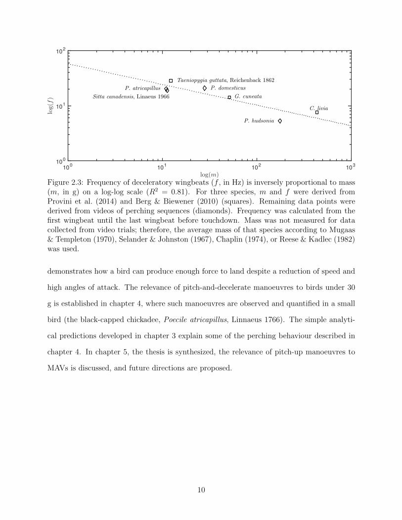
Wingbeat frequencies were calculated from the first deceleratory wingbeat to the final
wingbeat before touchdown for a number of perching sequences. Frequency decreases regu-
larly with body mass on a log-log scale (figure 2.3). An inverse proportionality between size
and stroke frequency is also observed in steady flight (Pennycuick, 1996)1. Pennycuick (1975)
attributed the reduction of frequency with increased mass to minimum lift requirements and
the scaling of muscle power to wing inertia. Similar arguments likely apply to the scaling of
frequency with mass in perching manoeuvres.
In these video sequences, no gliding-type pitch-up manoeuvres similar to figure 2.2 were
observed in any bird less than 100 g. This suggests that rapid pitch-up manoeuvres in
small birds differ from large birds. The scaling of wingbeat frequency with mass may be
responsible.
Smaller birds need to flap frequently to maintain lift, and birds of mass < 30 g with short,
rounded wings seldom glide, preferring instead to use a bounding-flight pattern (Tobalske
et al., 2007). Any dynamic changes in angle of attack must therefore occur during power
strokes with limited duration, whereas larger birds can change wing shape and orientation
in a slow gliding approach (Carruthers et al., 2007).
To explore physical mechanisms of force generation in a pitch-and-decelerate manoeuvre,
an experimental investigation is performed on a pitching airfoil in chapter 3. A simple ana-
lytical model, developed from the perspective of pitch-up as a rapid area change mechanism,
1In reality, Pennycuick (1996) showed that flapping frequency scales with a multiplicity of morphologicalfactors, and observed a small positive proportionality with mass, holding other variables constant. However,wing span (S) and area (A) scale negatively with stroke frequency (Pennycuick, 1996), and since S and Aincrease strongly with mass (Taylor & Adrian, 2014), a general trend of decreasing stroke frequency withincreasing mass is expected.
9
log(m)10
010
110
210
3
log(f)
100
101
102
P. atricapillus P. domesticus
Sitta canadensis, Linaeus 1966
P. hudsonia
C. livia
Taeniopygia guttata, Reichenback 1862
G. cuneata
Figure 2.3: Frequency of deceleratory wingbeats (f , in Hz) is inversely proportional to mass(m, in g) on a log-log scale (R2 = 0.81). For three species, m and f were derived fromProvini et al. (2014) and Berg & Biewener (2010) (squares). Remaining data points werederived from videos of perching sequences (diamonds). Frequency was calculated from thefirst wingbeat until the last wingbeat before touchdown. Mass was not measured for datacollected from video trials; therefore, the average mass of that species according to Mugaas& Templeton (1970), Selander & Johnston (1967), Chaplin (1974), or Reese & Kadlec (1982)was used.
demonstrates how a bird can produce enough force to land despite a reduction of speed and
high angles of attack. The relevance of pitch-and-decelerate manoeuvres to birds under 30
g is established in chapter 4, where such manoeuvres are observed and quantified in a small
bird (the black-capped chickadee, Poecile atricapillus, Linnaeus 1766). The simple analyti-
cal predictions developed in chapter 3 explain some of the perching behaviour described in
chapter 4. In chapter 5, the thesis is synthesized, the relevance of pitch-up manoeuvres to
MAVs is discussed, and future directions are proposed.
10
Chapter 3
Unsteady dynamics of rapid perching manoeuvres
Abstract
A perching bird is able to rapidly decelerate while maintaining lift and control, but the
underlying aerodynamic mechanism is poorly understood. In this work we perform a study
on a simultaneously decelerating and pitching airfoil section to increase our understanding
of the unsteady aerodynamics of perching. We first explore the problem analytically, de-
veloping expressions for the added-mass and circulatory forces arising from boundary-layer
separation on a flat-plate airfoil. Next, we study the model problem through a detailed series
of experiments at Re = 22000 and two-dimensional simulations at Re = 2000. Simulated
vorticity fields agree with Particle Image Velocimetry measurements, showing the same wake
features and vorticity magnitudes. Peak lift and drag forces during rapid perching are mea-
sured to be more than 10 times the quasi-steady values. The majority of these forces can be
attributed to added-mass energy transfer between the fluid and airfoil, and to energy lost to
the fluid by flow separation at the leading and trailing edges. Thus, despite the large angles
of attack and decreasing flow velocity, this simple pitch-up manoeuvre provides a means
through which a perching bird can maintain high lift and drag simultaneously while slowing
to a controlled stop.
3.1 Introduction
Birds execute precise manoeuvres, such as banking, braking, takeoff and landing, allowing
them to navigate dense forests and urban environments. Micro Aerial Vehicles (MAVs) are
contemporary flying machines operating on the same scale as small birds, and are designed to
11
carry out remote sensing and small payload delivery tasks in cluttered airspaces. Mimicking
the manoeuvrability of birds, particularly the ability to land safely on narrow platforms,
would allow them to complete these tasks effectively and efficiently. Though recent advances
have been made in designing MAVs that can land on a perch (Doyle et al., 2011; Moore
et al., 2014; Reich et al., 2009), existing MAVs still fall short in achieving the control, speed
and precision of natural flyers in landing manoeuvres.
Birds are tremendously adept at controlled, fast landings. Provini et al. (2014) observed
that zebra finches are able to decelerate from 15 to 7 body lengths per second in 0.15
seconds, entirely through aerodynamic means. Though the exact kinematic motion used
by birds in perching manoeuvres varies between species (Berg & Biewener, 2010; Provini
et al., 2014), one relatively simple motion is for a bird to pitch its wings continuously from
near-horizontal to approximately 90 angle of attack. Carruthers et al. (2007) observed this
motion in a Steppe Eagle and noted that the eagle gained altitude quickly during the landing
phase, implying that large lift was produced. However, steady-state analysis predicted that
the bird would lose lift at high angles of attack due to stall effects and reduced airspeed
(Carruthers et al., 2010). When decelerating most rapidly and gaining height, the eagle
entered a “rapid pitch-up phase”, in which it increased its angle of attack quickly while
simultaneously spreading its wings.
To model the aerodynamics of the pitch-up wing motion in landing birds, we consider an
airfoil that rapidly increases its angle of attack while simultaneously decelerating. Though
bird flight and landing is a three-dimensional problem, two-dimensional flow topologies often
dominate in highly-unsteady manoeuvres, as was shown by Garmann et al. (2013), and so
we restrict ourselves to the two-dimensional pitch-up problem.
When an airfoil pitches to high angles of attack, its frontal area rapidly increases. Rapid
frontal area change of bodies in acceleratory manoeuvres results in significant added-mass
effects, notably the recapture of added-mass energy as demonstrated by Weymouth & Tri-
12
antafyllou (2012) in a shrinking cylinder and Weymouth & Triantafyllou (2013) in a squid-like
deflating body. Rapid area change can also affect boundary-layer vorticity, causing sudden
global shedding of vorticity in a vanishing airfoil (Wibawa et al., 2012) and annihilation of
boundary-layer vorticity in a shrinking cylinder (Weymouth & Triantafyllou, 2012).
These above studies have all looked at the fluid dynamics of a body with rapidly-
decreasing area. However, the case of a body with rapidly-increasing frontal area has seen
comparatively little attention, despite the potential to inform biological and technological
designs. We show that the case of a pitching and decelerating airfoil manipulates added-
mass forces in a similar way to other rapid area change problems, but here the rapid increase
in area bears unique performance challenges. Additionally, the rotation of the body pro-
duces lift and dynamic forces from boundary-layer separation, which have hitherto not been
considered in rapid area change problems.
To study the unsteady dynamics of pitch-up during stopping manoeuvres, we first de-
velop a low-order analytic model for the lift and drag force-history on an airfoil performing
simultaneous pitch and deceleration. Such a model provides two benefits: (a) it identifies
the salient features of the flow in order to understand physical mechanisms, and (b) it may
be used to predict forces for MAV control at low computational cost.
Next, a complete set of numerical simulations and experimental studies are performed.
The results demonstrate that a high-speed pitch and deceleration manoeuvre produces re-
markable instantaneous lift and drag forces. By examining these results in the context of
the analytic model, we determine that the majority of these forces can be attributed to (i)
added-mass energy transfer between the fluid and airfoil, and (ii) to energy dissipated into
the fluid by boundary-layer separation at the leading and trailing edges. These effects com-
bine to achieve instantaneous and integrated forces compatible with the perching abilities of
birds.
13
3.2 Analytic arguments
We first develop an analytic model of the forces produced during a pitch-up and stop ma-
noeuvre to understand mechanisms of lift and drag generation in perching. Recent studies
(Ol et al., 2009; Baik et al., 2012; Pitt Ford & Babinsky, 2013) have shown that classical po-
tential flow theory from Theodorsen (1935), von Karman & Sears (1938) and Wagner (1925)
can provide reasonable predictions for the force histories of unsteady airfoils, even for low-Re
cases with pronounced boundary-layer separation. These models have explanatory power as
well, as they allow simple decomposition of the added-mass and circulatory forces. However,
these potential flow models assume a small angle of attack and a planar wake (Theodorsen,
1935; von Karman & Sears, 1938; Wagner, 1925), assumptions that are violated with rapid
pitch-up to high α.
In this study we use an added-mass model valid for arbitrary angles of attack and pitch
rate and derive a circulatory force model for highly-separated flows around non-oscillatory
airfoils. The combined model has no free parameters, being dependent only on the prescribed
kinematics of the pitching and decelerating airfoil.
3.2.1 Model problem description and the shape change number
Consider an airfoil with chord length c that is initially at an angle of attack α = 0 and
moving at a constant forward velocity U0. As a simple model of a bird’s wing during perching
manoeuvres, this airfoil section is made to rapidly rotate perpendicular to the translation
direction, that is to α = 90, while simultaneously decelerating to a full stop over time period
T . This system and its kinematics are sketched in figure 3.1.
We parameterize the magnitude of the geometry change of the system with the shape
change number
Ξ =V
U0
, (3.1)
where V ≡ c/T is the average speed at which the frontal width of the airfoil increases over
14
(a)
c
cx∗pα(t)
c(1 − x∗p)α
U(t)
0 0.5 1
0
0.5
1
t∗
(b) U/U0 2α/π
Figure 3.1: (a) A diagram showing the NACA0012 airfoil section with chord c and pivotpoint marked by a black dot at a distance cx∗p from the leading edge. The instantaneousangle of attack α(t) and velocity at the pivot U(t) are prescribed. (b) The kinematics used inexperiments and simulations, plotted as a function of non-dimensional time t∗ = t/T , whereT is the time period of the manoeuvre. The velocity is scaled by the initial value U0, whilethe angle is scaled by the final value π/2 radians. α is varied with a cycloidal function givenin equation (3.6).
the course of the manoeuvre. Defining the inline deceleration as U = U0/T and substituting,
we have Ξ = V 2/(Uc), matching the definition of shape change number in Weymouth &
Triantafyllou (2013). The parameter Ξ acts as a measure of the unsteadiness of the problem,
similar to the reduced frequency, k = πfc/U0, where f is a circular frequency. We choose to
use Ξ in this work to emphasize that the motion is not cyclic and that the change in frontal
area is fundamental to the perching problem.
For an airfoil rotating from α = 0 to 90 and simultaneously decelerating from U = U0
to 0 in time T , the magnitude of α, α and U can be estimated as
α ∝ 1
T=U0
cΞ, |α| ∝ 1
T 2=U2
0
c2Ξ2, U ∝ U2
0
cΞ (3.2)
so long as U and α are continuous functions in time. The relations given by (3.2) show that
Ξ parameterizes the rate of rotation, rotational acceleration and translational acceleration.
15
3.2.2 Added-mass manipulation through frontal area change
This change in frontal area has pronounced consequences on the added-mass forces produced
during the manoeuvre. These can be described from very simple relations, and merit a brief
discussion for readers unfamiliar with the topic.
Consider a body accelerating in one dimension but allowed to modify its frontal area in
time. As the body expands, it displaces more fluid, effectively increasing its added mass.
Conversely, a reduction in frontal area would decrease the added mass in time. The one-
dimensional added-mass force can be written as
FAM = − ∂
∂t(maU) = −maU −maU (3.3)
wherema is the instantaneous added-mass of the body. The terms on the right hand side arise
respectively from the rate of change of the added mass (maU) and from the acceleration of
the added mass (maU). Weymouth & Triantafyllou (2013) found that the added mass of an
accelerating prolate spheroid decreased during body deflation (ma < 0). This had a twofold
effect in view of equation (3.3). The first was in achieving additional thrust by recovering
added-mass energy (the −maU term). The second was in reducing parasitic drag throughout
the manoeuvre (the −maU term). Both effects were beneficial for the performance goal of
high acceleration.
However, there is a tradeoff for an expanding body when deceleration is desired. On
the one hand, addition of added-mass from frontal area expansion (ma > 0) would create
drag through −maU . But this would also increase the total added mass in time, making it
difficult to stop the body late in the manoeuvre by producing a net thrust through −maU .
The sudden change in the direction of forces would tend to yield an uncontrolled perching
manoeuvre, which is not observed (Green & Cheng, 1998; Berg & Biewener, 2010; Carruthers
et al., 2007). In the next two sections we extend the simple one-dimensional force model
equation (3.3) by discussing the effects of rotation on the added-mass force, and by modelling
the circulation forces created through the production of vorticity.
16
3.2.3 The added-mass force
The general added-mass force normal to a flat-plate airfoil in translation and rotation at
general angles of attack can be developed in a number of ways. The general boundary
function method of Milne-Thomson (1968) can be applied to give the potential solution
φ for the case of a rotating and accelerating flat-plate, from which the added-mass force
coefficient is determined to be
CFφ =πc
2U20
[α cos(α)U + sin(α)U + cα(1/2− x∗p)
](3.4)
where cx∗p is the distance from the leading edge of the airfoil to the pivot location. Xia &
Mohseni (2013) use an alternative rotating reference frame argument to develop the same
added-mass force expression. In the context of equation (3.3), the first term in brackets in
equation (3.4) arises from the time rate of change of added mass, and the second from linear
acceleration of added mass. The final term arises from rotational acceleration absent in the
one-dimensional analogy.
For the perching manoeuvre, we apply the relations given by (3.2) and see that the
added-mass force in equation (3.4) should scale by no more than Ξ2. We also note that the
added-mass force disappears as Ξ → 0 (the quasi-steady limit), as expected.
We next study equation (3.4) through a prescribed set of kinematics representing si-
multaneous deceleration and pitch-up to large α, relevant to perching manoeuvres in birds
(Carruthers et al., 2007):
U = U0(1− t∗) (3.5)
α(t) =π
2
[t∗ − sin(2πt∗)
2π
](3.6)
where t∗ = t/T = tV/c is the non-dimensional time (0 6 t∗ 6 1). We also set x∗p = 1/6. The
resultant added-mass lift and drag
Clφ = CFφ cosα (3.7)
Cdφ = CFφ sinα (3.8)
17
0 0.5 1
−2
−1
0
1
2
3
4
5
C l
t∗
circulatory
non-cir-
culatory
Ξ= 1/2
Ξ= 1/4
Ξ= 0
0 0.5 1
−2
−1
0
1
2
3
4
5
Cd
t∗
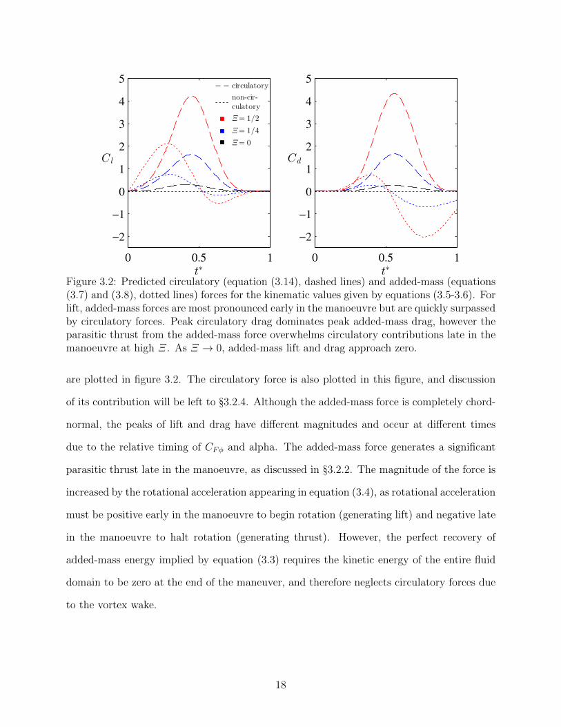
Figure 3.2: Predicted circulatory (equation (3.14), dashed lines) and added-mass (equations(3.7) and (3.8), dotted lines) forces for the kinematic values given by equations (3.5-3.6). Forlift, added-mass forces are most pronounced early in the manoeuvre but are quickly surpassedby circulatory forces. Peak circulatory drag dominates peak added-mass drag, however theparasitic thrust from the added-mass force overwhelms circulatory contributions late in themanoeuvre at high Ξ. As Ξ → 0, added-mass lift and drag approach zero.
are plotted in figure 3.2. The circulatory force is also plotted in this figure, and discussion
of its contribution will be left to §3.2.4. Although the added-mass force is completely chord-
normal, the peaks of lift and drag have different magnitudes and occur at different times
due to the relative timing of CFφ and alpha. The added-mass force generates a significant
parasitic thrust late in the manoeuvre, as discussed in §3.2.2. The magnitude of the force is
increased by the rotational acceleration appearing in equation (3.4), as rotational acceleration
must be positive early in the manoeuvre to begin rotation (generating lift) and negative late
in the manoeuvre to halt rotation (generating thrust). However, the perfect recovery of
added-mass energy implied by equation (3.3) requires the kinetic energy of the entire fluid
domain to be zero at the end of the maneuver, and therefore neglects circulatory forces due
to the vortex wake.
18
3.2.4 Circulatory forces
von Karman & Sears (1938) demonstrated that an airfoil wake and bound circulation could
be modeled as a superposition of equal strength, counter-rotating, point-vortex pairs. Each
vortex pair in two dimensions has an associated hydrodynamic impulse,
I = Γ z × r (3.9)
where Γ is the circulation of one of the vortices, z is a unit vector pointing normal to the
plane, and r is the displacement vector from the positive to negative vortex centre. Since the
circulatory force is related to the fluidic impulse by F γ = −ρdIdt
, this results in the following
relation for the circulatory contributions to forces on the body:
F γ = −ρΓ z × r − ρΓ z × r. (3.10)
Equation (3.10) shows that vortex forces can be altered through the addition or elimination
of circulation to or from the vortex dipole (Γ ) and by the convection of one vortex relative
to the other (r).
Analysis of the convective term in equation 3.10 is generally either accomplished by
assuming the wake is stationary relative to the undisturbed fluid, which leads to a lift pro-
portional to UΓ as in von Karman & Sears (1938), or by numerically tracking the distribution
of vorticity in the wake. As the transient perching flow is certain to be non-stationary, and
as the goal of the model is to develop an understandable description of the forcing to com-
plement further numerical and experimental testing, neither of these options is satisfactory.
Moreover, in the limit of a very high-speed manoeuvre it is reasonable to assume that the
flow simply will not have time to convect significantly, making this term negligible. Whereas
in the limit of a very slow manoeuvre with significant vortex shedding, the average value of
Γ in the wake will tend to zero, and therefore so will the mean convective force.
Therefore, for simplicity, we focus solely on the generation term. Pitt Ford & Babinsky
(2013) showed that net bound circulation was negligible for a flat-plate airfoil undergoing a
19
Figure 3.3: (Colour online) Sketch of the circulation production model. Velocity on thepressure side increases an amount equal to U⊥ while the separated fluid on the suction sidedoes not. This differential speed leads to a circulation per unit length γ = ∆u‖ = U⊥ atthe trailing edge. The negative vorticity in the wake, shown here as a blue line, increases inlength at the trailing edge at a rate equal to the trailing-edge speed: ds
dt= Ute. This results
in the total rate of change of circulation Γ = dΓds
dsdt
= UteU⊥. The circulation of the LEVincreases by an equal and opposite amount in accordance with Kelvin’s Theorem.
rapid acceleration; nearly all circulation was contained in the trailing edge wake and LEV.
For this reason, we suppose that all circulation is added to the flow at the leading and trailing
edges such that at the instant that vorticity is added to the flow, the two small resulting
vortices are separated by one chord length (figure 3.3). From equation (3.10), the resultant
force per unit length due to the generation of vorticity is
Fγ = −ρcΓ (3.11)
where Γ is the rate of (absolute) circulation shed into the flow at one edge and the direction
of force is normal to the chord towards the suction side.
We can estimate the production of circulation at the trailing edge of the airfoil by as-
suming that the fluid is detached on the suction side, such that the chord-normal component
of the velocity u⊥ only slowly decays with increased distance from the foil. In contrast, the
velocity field on the high-pressure side will quickly decay as in the potential flow solution.
Incompressibility of the flow therefore requires that the tangential velocity u‖ on the high
20
pressure side increases an amount equal to the normal velocity of the airfoil whereas the
suction side does not (figure 3.3). The velocity difference across the airfoil implies the fluid
in the region of the trailing edge should be modelled as a vortex sheet with strength
γ = ∆u‖ = U⊥ (3.12)
where U⊥ is the velocity of the trailing edge of the airfoil normal to the chord. Over a time
dt this sheet streams off the airfoil as the trailing edge covers a distance ds = Utedt. As
dΓ = γds, the production of circulation in the fluid is therefore
Γ = UteU⊥. (3.13)
From equation (3.11), this results in a force coefficient of
CFγ =2UteU⊥U2
0
. (3.14)
It is informative to expand these speeds in terms of the airfoil kinematics. We have
Ute =√U2 + 2Uη∗pcα sinα + η∗2p c
2α2 (3.15)
U⊥ = U sinα + η∗pcα (3.16)
η∗p ≡ 1− x∗p. (3.17)
Since α ∝ Ξ from equation (3.2), when Ξ 1 we have Fγ → ρc(η∗pcα)2, showing that
the translational component becomes negligible and that the production of circulation is
dominated by the rotation of the sharp trailing edge. Also note that as Ξ → 0, Fγ →
ρc sin(α)U2, showing that this circulatory model has a quasi-steady contribution. Unlike the
steady Kutta lift force, which is valid for attached flows at low angles of attack, this mean
force estimate is chord-normal and assumes fully detached flow.
Returning to figure 3.2, we note that the circulatory forces increase with Ξ, and the peak
lift and drag at Ξ = 1/2 are ∼ 10 times the steady-state values. Because the force is due
solely to the production of leading and trailing-edge vorticity, energy is transferred in only
one direction - from the airfoil to the wake.
21
3.2.5 The net force on an airfoil
By superimposing the added-mass (3.4) and circulatory (3.14) contributions we arrive at our
analytic model of the force coefficient:
CF =2
U20
[sin(α)U + cα(1− x∗p)
]√U2 + 2Ucα(1− x∗p) sin(α) + c2α2(1− x∗p)2
+πc
2U20
[α cos(α)U + sin(α)U + cα(1/2− x∗p)
]. (3.18)
This model depends only on two geometric and two kinematic (time-dependent) parameters:
the chord length c, the pivot point x∗p, the translational speed U(t), and the angle of attack
α(t).
We next present our experimental and numerical investigations of the two-dimensional
perching problem. We then discuss the results in the context of our simplified analytic model.
3.3 Experimental setup
To quantitatively assess the fluid dynamics induced by rapid perching, we performed a set
of experimental manoeuvres by varying Ξ using a towed NACA0012 airfoil. Forces on the
airfoil were measured directly, and the velocity field was measured using Particle Image
Velocimetry (PIV) to evaluate circulatory effects. All experiments were performed in a free-
surface towing facility at the University of Calgary. The water channel test section is 38.6
cm wide, and water level was maintained at a 42 cm depth. An aluminum NACA0012 airfoil
with 48 mm chord was positioned midway between the channel walls in a vertical orientation
(figure 3.4b and 2c) and pierced the free surface from above. The airfoil tip was 4 mm from
the bottom of the test section to reduce tip effects. Thus the airfoil had a submerged span
of 416 mm and an aspect ratio of 8.7. The high aspect ratio further justifies the assumption
of two-dimensional flow. A plastic skim plate of 112 mm diameter and 2 mm thickness was
secured to the airfoil and sat 3 mm below the water surface. This skim plate eliminated
the formation of free-surface funnel vortices. The airfoil was attached at one end to an ATI
22
Gamma force/torque balance. The force balance was attached to a two-phase stepper motor
with 0.9 step angle. The pitching axis was c/6 from the leading edge. The apparatus was
fixed to a Parker linear traverse, which ran along the length of the water channel.
The airfoil first established a steady-state condition at α = 0 and speed U0 = 0.45
m/s for at least 10 chord lengths before beginning rotation and deceleration. The Reynolds
number at the beginning of the manoeuvre is therefore Re = U0cν
= 22000, in the range
relevant for small, highly-manoeuvrable birds. The start of unsteady kinematics was synced
through an induction sensor at a fixed position on the traverse track, which detected the
passing traverse stage. The kinematics follow those shown in figure 3.1 and equations (3.5)
and (3.6).
3.3.1 Force measurements
Force measurements were taken at a 1000 Hz sample rate (16 bit sample depth). Recorded
force data was averaged across 10 trials for each test case. The force measurements were
repeated for the same kinematics once water had been drained from the channel in order
to measure the non-hydrodynamic inertia of the system. Force data was transformed from
an airfoil-fixed frame to a lab-fixed frame, and the inertia was subtracted. The transformed
data was further smoothed with a two-degree Butterworth low-pass filter. Filter frequency
cutoff was chosen as 4 Hz for Ξ = 1/32 and 10 Hz for Ξ = 1/2. Filter frequency cutoffs for
intermediate Ξ were determined by interpolating linearly between these values. This method
was found to best preserve peaks while eliminating noise. To avoid time-shifting of data,
a forward-backward filtering technique was used. Force measurements were synchronized
through the same induction sensor on the traverse track that triggered the deceleration.
Force measurements were also performed on the same airfoil at a constant speed (0.45
m/s) and constant angle of attack. α was varied between trials from 0 to 5 with 1
increments, and from 5 to 90 with 5 increments using a rotational stage (figure 3.4c).
The same measurements were performed for negative values of α to assess the symmetry
23
Figure 3.4: (a) PIV setup, showing a laser (A) projecting a laser sheet into the water tunnelfrom the side. The airfoil (C), attached to the traverse stage (B), was translated through thelaser sheet with prescribed kinematics. A Photron SA4 high-speed camera (D) filmed themanoeuvre through the glass bottom of the water channel. (b) The airfoil attachment usedfor PIV and force measurements. The airfoil (C) was attached to a 6-component force/torquebalance (F), which in turn was attached to a stepper motor (E). A plastic skim plate (G)prevented the formation of free-surface vortex funnels. The entire attachment was securedto the stage of a linear traverse (B), which sat on top of the water channel. (c) The airfoilattachment used for steady force measurements. The same airfoil (C), skim plate (G), andforce balance (F) attachment as the unsteady setup (b) was used. The force balance wasattached to a rotational stage (H), which in turn was secured to the traverse stage (B).
Table 3.1: Estimates of uncertainty and signal-to-noise ratios (SNRdb, in decibels) for liftand drag. σf is the measured standard deviation of the peak force coefficient across trials,and σt is the measured standard deviation of peak force time. Clmax and Cdmax are the peakaverage lift and drag coefficients, respectively.
of the setup. These measurements were used to make quasi-steady predictions (Ξ = 0).
Quasi-steady force coefficients were computed as
CF =2F
ρcS
U(α)2
U40
, (3.19)
where F is the measured force, U(α) is the speed of the airfoil at a particular angle of attack
in the unsteady case, and U0 is the starting speed.
To estimate the uncertainty of force measurements, the standard deviations of peak lift
and drag between trials at each shape change number were measured. Signal-to-noise ratios
were also calculated between filtered and ensemble-averaged data. Values are presented
in table 3.1. The measured standard deviations of peak forces do not exceed 8% of the
corresponding average peak value, and the measured standard deviations of the time of peak
forces do not exceed 4% of the corresponding period of deceleration and pitch.
3.3.2 Particle Image Velocimetry (PIV)
A 1 W, continuous-wave laser (λ = 532 nm) projected a laser sheet into a plane orthogonal
to the airfoil (figure 3.4a). This laser sheet was 21.1 cm above the water channel floor.
The water was seeded with silver-coated, hollow glass spheres of 100 µm diameter. These
particles have a Stokes number of approximately 2.4× 10⁻³, and therefore were assumed to
accurately follow the fluid flow. As the airfoil passed through the laser sheet, a Photron SA4
25
high-speed camera (1024× 1024 pixel resolution) captured images at 250 frames per second.
PIV data collection was synchronized with the same induction sensor on the traverse track
that triggered the profile deceleration.
Raw images were pre-processed with a min/max contrast normalization filter of size
14x14 pixels and a sliding-average subtraction filter of 50 pixel width. Velocity fields were
calculated with a multi-grid/multi-pass cross-correlation algorithm using DaVis software
(LaVision, v8.1.2). Velocity fields were averaged across 9 trials.
Based on the random error estimates of Raffel et al. (2007), pixel displacement uncertainty
is taken as δs = ±0.1px. Propagation of uncertainty through velocity and vorticity with 4-
pixel spacing between velocity vectors yields
δω∗ =δs
4∆t√n
c
U0
, (3.20)
where δω∗ is the non-dimensional uncertainty in vorticity, ∆t is the time interval between
frames and n is the number of trials. Given equation (3.20), the uncertainty in non-
dimensional vorticity for PIV measurements is estimated as δω∗ = ±0.2.
3.4 Numerical method
A set of two-dimensional incompressible Navier-Stokes simulations of the model perching
problem introduced in section 3.2 were used to provide high-resolution data with the exact
kinematics of this challenging test case. To further this aim, the Reynolds number based
on the initial steady speed U0 is set to Re = 2000 in these simulations to ensure the model
flow remains fully two-dimensional near the foil and the vortex structures remain clean and
easily identifiable.
The Boundary Data Immersion Method (BDIM), a robust immersed boundary method
suitable for dynamic fluid-structure interaction problems detailed in Weymouth & Yue (2011)
and Maertens & Weymouth (2015), was used for this purpose. Briefly, the full Navier-
Stokes equations and the prescribed body kinematics shown in figure 3.1 are convolved with
26
a kernel of support ε = 2h, where h is the grid spacing. The integrated equations are
valid over the complete domain and allow for general solid-body dynamics to be simulated.
Previous work has validated this approach for a variety of dynamic rigid-body problems such
as accelerating airfoils (Wibawa et al., 2012) and deforming-body problems (Weymouth &
Triantafyllou, 2013). In Maertens & Weymouth (2015) this method was validated against
stationary and flapping airfoil test cases at moderate Re and found to produce accurate and
efficient numerical solutions.
A non-inertial computational domain is used with dimensions 8c×8c, which translates and
decelerates with the body but does not rotate. All cases use the no-slip and no-penetration
boundary conditions on the solid/fluid interface. No-penetration conditions are applied on
the top and bottom walls and a convection exit condition is used. The coupled BDIM
equations are discretized using a finite-volume method (third-order convection and second-
order diffusion) in space and Heun’s explicit second-order method in time. An adaptive
time-stepping scheme is used to maintain stability. Figure 3.5 presents a grid convergence
study on the peak lift and drag coefficients for the Ξ = 1/4 test case. The results converge
with second-order accuracy overall and the difference in the solution between an extremely
fine reference grid (using 400 points along the chord) and a 200 point-per-chord grid is less
than 2% in lift and drag. The velocity, pressure and vorticity fields for these grids are
indistinguishable. This verifies the convergence of these viscous two-dimensional simulations
and the 200 points-per-chord grid is used for the remainder of the paper.
3.5 Results and discussion
In §3.5.1, we present velocity-field measurements from two test cases (Ξ = 1/4 and 1/2)
using data from PIV at Re = 22000 and BDIM simulations at Re = 2000. In §3.5.2, we
present results from force measurements and compare them to the low-order analytic model.
First, we compare instantaneous forces between Re at high Ξ and discuss differences in view
27
(a) Normalized peak error in CL
0.01
0.10
1.00
0.005 0.010 0.020 0.040h/c
(b) Normalized peak error in CD
0.01
0.10
1.00
0.005 0.010 0.020 0.040h/c
Figure 3.5: Normalized simulation error of the peak values of lift and drag coefficient forthe Ξ = 1/4, Re = 2000 test case as a function of the grid size h. The error is computedrelative to the values obtained using a fine c = 400h reference grid. The solid lines indicatesecond-order convergence with h and the dashed lines indicate first-order convergence.
of observed flow topology. Next, we compare the model to results from a large range of Ξ.
Finally, in §3.5.3 we present the time-averaged lift and drag generated during the manoeuvre
with applications to functional trade-offs in landing birds.
3.5.1 Velocity-field results
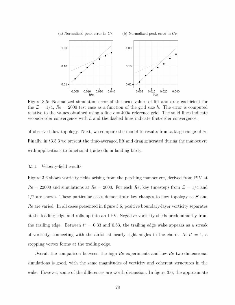
Figure 3.6 shows vorticity fields arising from the perching manoeuvre, derived from PIV at
Re = 22000 and simulations at Re = 2000. For each Re, key timesteps from Ξ = 1/4 and
1/2 are shown. These particular cases demonstrate key changes to flow topology as Ξ and
Re are varied. In all cases presented in figure 3.6, positive boundary-layer vorticity separates
at the leading edge and rolls up into an LEV. Negative vorticity sheds predominantly from
the trailing edge. Between t∗ = 0.33 and 0.83, the trailing edge wake appears as a streak
of vorticity, connecting with the airfoil at nearly right angles to the chord. At t∗ = 1, a
stopping vortex forms at the trailing edge.
Overall the comparison between the high-Re experiments and low-Re two-dimensional
simulations is good, with the same magnitudes of vorticity and coherent structures in the
wake. However, some of the differences are worth discussion. In figure 3.6, the approximate
28
Figure 3.6: PIV measurements (Re = 22000) and simulations (Re = 2000) of vorticity fieldsat Ξ = 1/4 (top) and Ξ = 1/2 (bottom). Black dotted lines represent the approximate x-position of the centre-of-mass of the starting vortex and LEV. In the higher-Re Ξ = 1/4 case,the starting vortex trails behind the LEV by a distance of x/c = 1.4 at t∗ = 0.67, whereasthe starting vortex trails less than x/c = 1.0 behind the LEV in the other cases. The whitearrows, shown at Re = 2000, point to a stagnation streamline that connects with the airfoilnear the trailing edge. At t∗ = 0.33, the stagnation streamline does not lie at the trailingedge. By t∗ = 0.67, the stagnation streamline has moved to the airfoil tip. The referenceframe translates such that the origin is fixed at the pivot point. The airfoil is translatingin the positive x-direction. Grey-shaded areas in PIV plots denote regions that have beenmasked due to shadowing effects or visual obstruction. Vorticity is non-dimensionalized byω∗ = ωc/U0.
29
distance between the centre of mass of the LEV and starting vortex are labeled. The LEV
remains close to the pivot axis and convects along with the airfoil. For Ξ = 1/4 and
Re = 22000, the starting vortex is approximately 1.4 chord lengths behind the pivot axis
by t∗ = 0.67. In contrast, at lower Re the trailing-edge wake is only ∼ 1 chord length from
the pivot axis at the same Ξ and time. The length of the wake is strongly influenced by the
positive x-velocity of the starting vortex induced by the LEV and other wake vortices. For
a given strength, a pair of diffuse vortices induce weaker velocities on one another (Saffman
& Szeto, 1980; Pierrehumbert, 1980). Figure 3.6 shows that the higher-Re wake vortices
and LEV are more diffuse due to turbulent transition and vortex breakdown. Therefore,
the difference in wake length is explained by turbulent diffusion of vorticity in the three-
dimensional, higher-Re cases, not present in the two-dimensional, lower-Re simulations.
The simulations also clarify some elements of the flow that are obscured in the PIV. A
stagnation streamline is observed in the lower-Re cases as the white region between counter-
clockwise (red) and clockwise (blue) vorticity near the trailing edge, and is marked with
a white arrow at t∗ = 0.33 and 0.67. At t∗ = 0.33, this stagnation streamline does not
lie at the trailing edge, therefore violating the steady Kutta condition. As discussed by
McCroskey (1982), the Kutta condition can break down in highly-unsteady manoeuvres,
and abrupt streamline curvature can be present in the trailing-edge region. We find that the
Kutta condition appears to be established by t∗ = 0.67. This is consistent with the results
of Pitt Ford & Babinsky (2013), who found that the Kutta condition is violated early in
an impulsive manoeuvre due to the presence of the starting vortex, but is established as
distance from the starting vortex increases.
3.5.2 Force history
The forces on the airfoil from the Re = 2000 simulations and Re = 22000 experiments for
shape change numbers of 1/8, 1/4 and 1/2 are shown in figure 3.7 along with the model
predictions from equation (3.18). In all cases, general trends predicted by the analytic
30
t∗0 0.5 1
Cd
-2
0
2
4
t∗0 0.5 1
Cl
0
2
4
6Re = 22000
Re = 2000
Model
Ξ = 1/2Ξ = 1/4Ξ = 1/8
Figure 3.7: A comparison between force results from experiments at Re = 22000 (solidlines), simulations at Re = 2000 (dotted lines), and model predictions (dot-dash lines) for1/8 6 Ξ 6 1/2. The magnitudes and timing of peaks in drag are similar between Re cases.The timing of peak lift is similar as well. However, magnitudes of lift are similar only in theΞ = 1/2 case. Model predictions are in close agreement with low-Re force histories.
model are observed: a single lift peak appears close to t∗ = 0.4, a drag peak appears close
to t∗ = 0.5, a thrust peak appears late in the manoeuvre, and the magnitudes of all peaks
increase with Ξ.
Overall, the model agrees with lower-Re lift at all Ξ, suggesting that added-mass forces
combined with boundary-layer separation at the leading and trailing edges are the dominant
mechanisms of lift generation in lower-Re cases. In the higher-Re cases, however, vortex
convection appears to be an important lift-generating mechanism. The vorticity fields shown
in figure 3.6 indicate that streamwise vortex convection is greater at Re=22000 than at
Re=2000 for Ξ = 1/4, and the force measurements support this by showing increased lift
forces on the airfoil for Ξ 6 1/4 relative to the simulations and the model. Again, the
differences in vortex convection between Re cases are attributed to turbulent diffusion at
higher Re not present in the simulation resulting in convective force which was neglected in
the analytic force model.
31
t∗0 0.5 1
Cd
-0.5
0
0.5
1
t∗0 0.5 1
Cl
-0.5
0
0.5
1
Re = 22000
Model
Ξ = 1/8Ξ = 1/16Ξ = 1/32Ξ = 0
Figure 3.8: Lift and drag coefficients in non-dimensionalized time, plotted for varying Ξ. Themagnitudes of forces increase with Ξ. At lower Ξ, results approach quasi-steady predictions(solid black line). The model is overlaid as a dot-dash line. Experiment agrees with themodel best at low shape change numbers. The Ξ = 0 case displays a peak lift at pre-stallangles of attack.
Drag histories compare well between the model, simulations, and experiment, particularly
in the large drag peak for t∗ < 0.75 when added-mass and boundary-layer separation are
the dominant mechanism of force generation. From 0.75 < t∗ < 1, the measurements and
simulations demonstrate the parasitic thrust forces predicted by the added-mass model. The
magnitude of the thrust measured for Ξ = 1/2 at higher-Re is larger than that predicted
by the combined model, but in line with the thrust predicted by the added-mass estimate in
equation (3.3). This indicates the model over-predicts the vortex drag late in the manoeuvre,
likely due to interaction effects between the LEV and trailing-edge wake as the airfoil comes
to a stop.
Figure 3.7 shows that the accuracy of the model in lift generally increases as Ξ increases
for higher-Re. In §3.2.4, we proposed that the model would also become more accurate
in the quasi-steady limit because of the von Karman vortex street which drives the mean
convective force to zero. To assess agreement as Ξ → 0, we performed force measurements
32
at Re = 22000 with shape change numbers varying from 1/8 to 0 (figure 3.8). As Ξ is
reduced, measured forces approach quasi-steady values at Ξ = 0. In the quasi-steady case,
note that increased ‘time’ in figure 3.8 corresponds to increased angle of attack via equation
(3.6), and the mean forces are shown scaled as in equation (3.3.1).
A continuation of the trends in figure 3.7 are observed in figure 3.8: single peaks in lift,
drag and thrust are observed, and the magnitudes of these force peaks continue to decrease
as Ξ decreases. As proposed, the model predicts the quasi-steady measurements well overall
as long as the angle of attack is sufficiently large to induce shedding from the leading and
trailing edge. The flow remains attached along the suction side of this NACA0012 airfoil
section below α ∼ 10 → t∗ ∼ 0.25, enhancing lift well above model predictions. At high
angles of attack vortices shed rapidly from the trailing and leading edges, the foil stalls and
the lift drops rapidly. Once this rapid shedding begins, the assumptions of the model are
satisfied, explaining the better agreement at large t∗. Similarly, in the Ξ = 1/32 case lift
drops off suddenly after reaching its peak and thereafter is closely predicted by the model.
The peak and decay in lift for Ξ = 1/32 occur at a higher angle of attack than for Ξ = 0,
which is a manifestation of dynamic stall, a phenomenon in which boundary-layer vorticity
remains attached beyond static stall angles of attack in pitching airfoils (McCroskey, 1982).
3.5.3 Time-averaged forces
Ultimately, the net forces produced over the course of a perching manoeuvre determine if
a flying bird or vehicle can safely land. To come to a complete stop, a bird of mass m
flying at an initial horizontal speed U0 must achieve a time-averaged drag of −mU0/T and
a time-averaged lift equal to its weight. Birds can and do supply some of the force required
to land from their legs at touchdown, but most of the momentum change is generated by
aerodynamic means (Provini et al., 2014).
Time-averaged lift and drag for 0 6 t∗ 6 1 are plotted against Ξ in figure 3.9, with lift
and drag coefficients derived from Re=2000 simulations, Re=22000 experiments, and model
33
Ξ
0 0.1 0.2 0.3 0.4 0.5
Cl
0
0.5
1
1.5
2
2.5
Re = 22000
Re = 2000
Model
Ξ
0 0.1 0.2 0.3 0.4 0.5
Cd
0
0.2
0.4
0.6
0.8
1
1.2
Figure 3.9: Time-averaged lift (Cl) and drag (Cd) are always positive and increase with Ξ.Time-averaged lift is greater than drag at higher shape change numbers due to added-massforces that contribute to lift but detract from drag (figure 3.2). Time-averaged lift is greaterat Re = 22000, compared to Re = 2000 results and model predictions, due to lift generationfrom vortex convection present in the higher-Re cases.
predictions. Minimum time-averaged lift and drag coefficients occur at Ξ = 0. Both lift
and drag increase as Ξ increases, the former more rapidly than the latter, and appear to be
unbounded. The minimum lift requirement is proportional to the constant value mg and can
be satisfied by increasing Ξ. The minimum drag requirement for a full stop is proportional
to Ξ, but since time-averaged drag is predicted to grow as Ξ2, this drag criteria can always
be met at high Ξ. This suggests that a bird can simply increase its pitch rate to meet the
minimum criteria of a perching manoeuvre, though the costs of fast pitch rates include large
torque requirements and high instantaneous loads on the wing.
The model predictions are in close agreement with Re=2000 time-averaged lift. At Re =
22000, the model is in best agreement with time-averaged lift at Ξ = 0 and 1/2. The
maximum error in the predicted lift force occurs at intermediate Ξ and high-Re, due to
neglecting the additional lift mechanism of vortex convection. Model predictions also agree
with lower-Re time-averaged drag and are slightly lower than higher-Re results at low Ξ.
The large thrust late in the Ξ = 1/2 experiment reduces the accuracy of the average for that
34
case.
The model predicts time-averaged lift is much higher than drag at larger Ξ. This is due
to added-mass forces that contribute to lift but detract from drag (figure 3.2). The large
differences in integrated lift and drag are amplified by increasing Re to 22000, due primarily
to lift generation from vortex convection. A landing bird may thus generate greater time-
averaged lift than drag during a pitch-up manoeuvre. This may help explain why the eagle
observed by Carruthers et al. (2007) would consistently approach its perch from below, and
exhibited a rapid increase in altitude during its pitch-up phase. As the authors of that
study suggested, this may be a means to aid deceleration by transferring kinetic energy to
potential energy. However, it may also be that the pitching manoeuvre necessary to generate
the required drag produces so much excess lift that an altitude correction is needed to avoid
overshooting the perch.
3.6 Summary and conclusions
In this study we investigate how high lift and drag can be generated through a controlled
pitch-up manoeuvre in the context of bird perching. As a simple perching model, we study
the aerodynamics of an airfoil that simultaneously decelerates and pitches to a high angle
of attack. The pitch rate and deceleration is parameterized by the shape change number,
Ξ, a ratio between the speed of frontal area expansion and initial translational speed. We
investigate differences in forces and vorticity fields as shape change number is varied from
0 to 1/2, using force measurements and Particle Image Velocimetry at Re = 22000 and
simulations using the Boundary Data Immersion Method at Re = 2000. A simple analytic
model that includes forces from added-mass effects and boundary layer separation at the
leading and trailing edges is derived and compared to the measurements.
The simulations and PIV measurements for Ξ = 1/4 and Ξ = 1/2 reveal that the wake
of the perching airfoil is dominated by a large leading edge vortex, which remains close
35
to the foil, and the trailing edge vorticity, which forms a vortex shear layer that rolls up
due to Kelvin-Helmholtz instability. The distance between the leading and trailing edge
structures is found to be greater than the chord length c in the Re = 22000 and Ξ = 1/4
case, indicating that vortex convection, neglected in the analytic model, is present in this
case. The trailing edge separation point was found to be located on the suction side of the
foil initially, only moving to the airfoil tip halfway through the manoeuvre, in agreement
with previous experiments.
Both experiments and simulations demonstrated that the lift and drag forces increase
super-linearly with Ξ, achieving peak values of Cl = 5.3 and Cd = 4.0 at Ξ = 1/2, which
are more than an order of magnitude larger than their steady-state peak values. The airfoil
is found to experience parasitic thrust at the end of the manoeuvre, but the average drag on
the airfoil is always positive and increases with Ξ.
Analogous to previous rapid area change studies, we find added-mass energy in the perch-
ing problem is transferred from the immersed body to the fluid as the frontal area and
added-mass increases, producing large lift and small drag. This energy is then recovered by
the airfoil late in the manoeuvre in the form of a parasitic thrust, which would be coun-
terproductive to a decelerating manoeuvre. However, a simple model of the vortex force
developed in this work predicts that the generation of circulation at the leading and trailing
edges dissipates enough energy into the wake to nearly overwhelm this parasitic thrust. We
find that the analytic model agrees best with force histories at lower Re, and with higher-Re
cases in the limits of quasi-steady and near-impulsive rotation. In particular, the effects of
vortex convection were found to be negligible after stall in near steady-state manoeuvres
and were overwhelmed by the production of vorticity in rapid manoeuvres. As these forces
can be difficult to estimate in transient flows, the simple kinematic model developed in this
work is of great utility.
The large forces observed suggest that pitching rates can be tuned to meet the demanding
36
lift and drag requirements of perching manoeuvres. Rapid pitch-up may therefore be a means
by which a landing bird can maintain lift while quickly braking to a controlled stop and could
be effectively applied in manoeuvrable micro-aerial vehicles in the near future.
Acknowledgements
The authors wish to thank the Natural Sciences and Engineering Research Council of Canada
and Alberta Innovates Technology Futures for financial support.
37
Chapter 4
Rapid area change from pitch-up manoeuvres in a
small perching bird
Abstract
Rapid pitch-up during perching manoeuvres has been highlighted as a mechanism to generate
large lift and drag, but pitching rates had not been measured in perching manoeuvres. We
measure pitch rates in a small, wild bird (Poecile atricapillus, Linnaeus 1766). While some
perching birds pitch gradually from one stroke to the next, members of P. atricapillus pitch
up rapidly in one wing stroke. Pitching rates were characterized by the shape change number,
a metric comparing the rate of frontal area increase to wing acceleration. Members of P.
atricapillus increase the shape change number during perching to dissipate energy quickly
in direct proportion to their total kinetic and potential energy as deceleration begins. The
linear relationship between dissipated energy and shape change number is in accordance with
simple analytical arguments developed for two-dimensional pitching and decelerating airfoils.
Members of P. atricapillus use a wing pitch-up manoeuvre during perching to generate large
forces and maintain lift and drag through rapid area change. It is suggested that similar
pitch-and-decelerate manoeuvres could be used to aid in controlled, precise landings in small
manoeuvrable air vehicles.
4.1 Introduction
Birds execute such diverse precision manoeuvres as banking, braking, takeoff and landing, in
order to navigate dense forests and urban environments. Micro Aerial Vehicles (MAVs) are
flying machines of a similar size as small birds, designed to carry out remote sensing tasks in
38
cluttered airspaces. Mimicking the manoeuvrability of birds, in particular the ability to land
on small platforms safely, would allow these vehicles to complete their objectives effectively
and efficiently. Though progress has been made in designing perching MAVs (Doyle et al.,
2011; Moore et al., 2014; Reich et al., 2009), existing MAVs fall short in achieving the control,
speed and precision of natural flyers in landing manoeuvres.
In order to perch, a bird must change its velocity from a cruising speed to a speed
close to zero. Birds simultaneously adjust their body and wing posture to become more
vertical (Carruthers et al., 2007; Berg & Biewener, 2010; Provini et al., 2014), as horizontal
postures reduce drag during cruising flight, but an upright posture facilitates a larger angle
of attack for deceleration. Carruthers et al. (2007) noted that the steppe eagle in their study
would perform a rapid pitch-up manoeuvre during perching sequences, where the angle of
attack would change smoothly from near-horizontal to near-vertical. However, steady state
aerodynamic analysis predicted a loss of lift at high angles of attack, due to stall effects
combined with a reduction of airspeed (Carruthers et al., 2010).
In chapter 3, it was shown that a rapidly-pitching airfoil can achieve large instantaneous
and integrated lift and drag, even while decelerating to a stop and pitching to a 90 angle
of attack. The pitch rate was parameterized through the shape change number, Ξ. Forces
increased as Ξ2 through a combination of added-mass energy transfer and vorticity genera-
tion. These results suggest that rapid area change through dynamic pitching helps generate
the forces required by a perching bird to quickly decelerate and stay aloft.
Though prior works have noted body and wing pitch-up in perching birds (Carruthers
et al., 2007; Berg & Biewener, 2010; Provini et al., 2014), no existing studies have reported
wing pitching rates in perching birds or demonstrated that the resulting area change is
associated with large forces on the body. In this work, we demonstrate fast pitch rates during
perching in a small, wild bird (the black-capped chickadee; Poecile atricapillus Linnaeus
1766), parameterize these rates in terms of the shape change number, and show that members
39
of P. atricapillus alter their shape change number as the demands of the perching manoeuvre
increase, implying that rapid area change through dynamic pitching is a kinematic tool that
can be tuned to meet the needs of small landing air vehicles.
4.1.1 Energy dissipation through rapid area change
A change in angle of attack increases the frontal area of a wing. This is an example of rapid
area change, in which a body in fluid exhibits a rapid expansion or contraction of area while
moving. Weymouth & Triantafyllou (2013) showed that rapid area change is characterized
by the shape change number,
Ξ =V 2
aL(4.1)
where V is the outward or inward velocity of area change, a is the body acceleration and L
is a body length scale. Weymouth & Triantafyllou (2013) demonstrated that by changing
the shape change number, the added mass, boundary-layer vorticity and forces on the body
can be modified dramatically.
These arguments were extended in chapter 3 to a two-dimensional, rapidly-pitching airfoil
decelerating from initial velocity U0 to a halt. Substitution of kinematic parameters into
equation 4.1 revealed that
Ξ =V
U0
, (4.2)
showing that the shape change number is a measure of the change in frontal area relative
to a characteristic change in forward velocity. The parameter Ξ acts as a measure of the
unsteadiness of the problem, similar to the reduced frequency, k = πfc/U0, where f is a
circular frequency. As in chapter 3, Ξ is chosen in the present study to emphasize that
the manoeuvre of interest is not cyclic and the change in frontal area is fundamental to the
perching problem.
As the metric (4.2) was constructed in two dimensions, it requires some modification to be
applied to a three-dimensional perching bird. We derive an analogous shape change number
40
in section 4.3.2, after establishing the characteristic perching behaviour of P. atricapillus.
As rapid area change is an effective means to shed energy, we expect a relationship
between the shape change number used by these birds and the energetic demands of a
perching manoeuvre. Once the bird has perched successfully, its kinetic and gravitational
potential energy relative to the perch are both zero. The total change in energy is therefore
∆E = mg∆z +1
2mU2
0 , (4.3)
where m is the bird’s mass, U0 the initial speed of its center of mass (CoM) and ∆z the height
of its CoM relative to the perch. In principle, any amount of energy could be dissipated with
the smallest force, given sufficient time. In practice, however, a bird needs to stay airborne
until it lands. Slow deceleration requires longer periods of sustained lift, costing metabolic
energy.
Whereas a large bird may sustain lift by gliding, a small bird must flap its wings frequently
to stay aloft. Thus, while the eagle observed by Carruthers et al. (2010) could pitch its wings
gradually during a perching manoeuvre, a small bird such as P. atricapillus has only a short
time to pitch before it must flap again to stay airborne. Since rapid area change through
pitching is a highly-effective means to quickly shed energy into the surrounding fluid, it
would be ideal to shed most of the energy quickly during a rapid pitch-up manoeuvre.
In chapter 3, a perching and decelerating airfoil produced drag as D ∝ Ξ2, while the
translational distance was d ∝ 1/Ξ, due to higher rates of deceleration. The total energy
dissipated in such a manoeuvre scales as
∆E ∝ dD ∝ Ξ. (4.4)
Therefore, we expect the shape change number used by these small birds to increase linearly
with the energetic requirements of perching manoeuvres.
41
1.4 m
1.2 m
3 m
Figure 4.1: A diagram of the setup used in data collection. A feeder was placed at thecentre of an enclosure, which was open on two ends. Four cameras were positioned aroundthe enclosure, forming effectively two reconstruction volumes: a smaller control volume forimproved resolution of the pitch-up manoeuvre (green) and a larger control volume to capturethe entire perching sequence (blue).
4.2 Experimental setup
A rectangular enclosure, 3 m long, 1.2 m wide and 1.4 m high was built to encourage birds
to approach from a consistent direction (figure 4.1). Two sheets of white polyethylene were
attached to the long sides, and two layers of 1” hexagonal wire mesh was fixed on the upper
surface. A plastic tray feeder was set 0.9 m above the ground in the centre of the enclosure,
and filled with commercially-available birdseed. The two smaller faces on opposite sides of
the enclosure were left open. As Green & Cheng (1998) showed that birds will manoeuvre
differently to land on a novel perch, filming began 11 days after the feeder was placed and
five days after the enclosure was finished, allowing the birds time to acclimate to the setup.
Four Casio EX-ZR700 high-speed cameras were arranged around the enclosure to allow
multiple views of perching sequences. The cameras recorded colour images at 480 frames
per second in 13-minute intervals while birds flew to the perch freely. Camera frame offsets
were calculated based on a flashing LED. Camera positions were calibrated using the Sparse
42
Bundle Adjustment algorithm packaged in the MATLABTM script easyWand (Theriault
et al., 2014). A 10 cm calibration wand was waved through the reconstruction volume as a
calibration target. The reference frame was aligned to gravity by measuring the acceleration
of an object falling through the reconstruction volume. Calibration reconstruction error was
estimated as ∼ 1 mm, based on the standard deviation of the wand length for all wand
images, and synchronization error was estimated as ±1 ms.
Perching sequences were digitized manually using the MATLABTM script DLTdv5, writ-
ten by Hedrick (2008). Details of the body parts digitized can be found in figures 4.2B and
4.2C. After digitization, position data was processed using custom MATLABTM scripts (Ap-
pendix C). Three-dimensional kinematic position data was smoothed with a second-order
low-pass Butterworth filter with 50 Hz cutoff. Velocities and accelerations were computed
where x, u and a refer to position, velocity and acceleration vectors, respectively, and ∆t is
the time increment between frames.
The CoM was taken as the average position between rump tip and beak (figure 4.2). The
rump tip was used because it was relatively easy to distinguish in all trials. However, as
both rump tip and head are mobile relative to the center of mass, artifacts in acceleration
can appear as the bird adjusts its body orientation. To compensate for this somewhat in
instantaneous CoM acceleration plots, the true rump location (point 2b in figure 4.2C) was
digitized for one trial where it could be distinguished easily. However, movement of the head
can still induce artifacts of CoM acceleration, and these will be noted where they appear in
the results.
As a metric for the dynamic demands of a perching manoeuvre, we estimated the bird’s
initial total energy as described in equation 4.3. As the mass of each bird was not measured,
43
we assumed a simple geometric scaling of body length to mass (m ∝ L3). To attain the
correct units of mass in equation 4.3, L3 was multiplied by the arbitrary density 1000 kg/m3.
Body length was taken as the mean distance between beak and rump tip from the end of
the ballistic phase up to the straightening of the arm. U0 is the average CoM speed from the
end of the ballistic phase (t0) to when the wrist is first straightened (t1). ∆z is the height
of the CoM relative to the perch at t1, and g is the acceleration due to gravity (9.8 m/s2).
4.3 Results and discussion
Eleven perching sequences were analyzed from two filming sessions five days apart. Based
on these sequences, the qualitative perching behaviour is described in section §4.3.1. An
extension of the two-dimensional shape change number as presented in chapter 3 to these
perching manoeuvres is established in §4.3.2, followed by quantitative kinematic results.
4.3.1 Overview of perching behaviour in P. atricapillus
Members of P. atricapillus exhibit a ballistic phase before beginning rapid deceleration (fig-
ure 4.2A; see supplemental video S1 for a representative perching sequence). This phase is
characterized by the wings folding tightly around the body and the tail being fully closed,
with no apparent active force generation. The bird then enters a deceleration phase, char-
acterized by changes in body orientation and wing and tail kinematics. At the start of this
deceleration phase, the wings rapidly extend with a forward power stroke. The body also
shifts from a horizontal orientation to a more vertical orientation. The tail feathers open
as the body posture becomes more vertical. After the first forward stroke, the bird per-
forms a rearward recovery stroke and begins a sequence of between one and four subsequent
power-recovery stroke cycles before touchdown (median 2, mean 2.4, standard error 0.28).
Power strokes from the wing cause a torque about the bird’s center of mass, as made
evident by the rotation of the body into a vertical position following the first power stroke in
44
Figure 4.2: (A) A compound image from a single perching sequence, showing (left to right)the end of the ballistic phase (t0), the first frame where the wrist straightens (t1), and thefinal frame before the wrist flexes (t2). The shape change number is calculated between t1and t2. x′ denotes the displacement vector of the center of mass from t1 to t2. The anglebetween x′ and the horizontal denotes the angle by which the vertical is rotated to formz′. Angle of attack is measured relative to the plane whose normal is z′. (t0 → t1 : 38 ms.t1 → t2 : 23 ms.) (B) Video still at t1. Digitized points are shown as red circles. Points 1and 2 are the beak and rump tip, respectively. The average of points 1 and 2 was used as aproxy for the CoM. Point 3 is the wing tip, distinguished as the next-to-last primary feather.Points 4 and 5 were used to measure wing chord and angle of attack and are, respectively, theshoulder and the tip of the secondary feather most proximal and posterior to the bird. (C)Video still at t2. Note the more vertical orientation of both body and wing as compared to(B). The approximate location of the left wrist is shown as a blue arrow. For instantaneousCoM acceleration plots, the true rump location (point 2b) was digitized for one trial whereit could be distinguished easily.
45
the deceleration phase. However, further rotation of the body generally ceases with further
forward wing strokes when the tail is fully expanded. This suggests that the tail counteracts
the torque produced by the wings while also producing greater drag.
In all observed perching sequences, the birds performed the majority of body reorientation
in the first power stroke. This is in contrast to rock pigeons, diamond doves and zebra finches
(Berg & Biewener, 2010; Provini et al., 2014), which alter their body angle continuously
during the perching sequence. Since this first stroke is associated with the largest change in
posture, and therefore presumably the largest pitch rates, we analyzed this stroke in detail
to quantify the shape change number and associated forces.
4.3.2 A three-dimensional analogue to the two-dimensional shape change number
Here we extend the two-dimensional shape change number for a pitching and decelerating
airfoil (equation 4.1) to an analogous metric relevant to the first perching power stroke
described above. During the first stroke, there are three ways in which members of P.
atricapillus can use control surfaces to change frontal area: (1) extending the wings as they
unfold from the body, (2) expanding and pitching the tail and (3) pitching the wings. The
latter is most similar to earlier work on two-dimensional pitching airfoils, and so is most
amenable to comparative analysis. The first two effects merit future study but are beyond
the scope of this thesis.
For P. atricapillus, the majority of wing pitching occurs after the wings are fully extended.
Once the wing is extended, its change in planform shape appears minimal, fortuitously
separating the effects of area change due to pitching from wing expansion. Therefore, Ξ
is calculated from the timestep where the wrist is first straightened (t1) to the timestep
immediately before the wrist flexes again (t2; see figure 4.2). The pitch angle to the horizontal
is measured at these two points (α1 and α2, respectively). Taking the chord length, c, and
46
setting T = t2 − t1, the shape change velocity is then
V =c(sinα2 − sinα1)
T. (4.7)
The shape change number requires a characteristic translational velocity change (∆U).
Between t1 and t2, the wing is relatively stiff and performs a sweeping motion that is effec-
tively a solid body rotation about the shoulder. The average chord-wise airspeed across the
wing is approximately equal to the speed of the wing, normal to the span, at the midpoint
between shoulder and wingtip. We calculate these airspeeds at t1, t2, producing U1 and U2
respectively. Conveniently, the wings are decelerating from t1 to t2 while pitching up, similar
to a two-dimensional pitch-and-decelerate manoeuvre. Thus, the deceleration analogous to
this two-dimensional case is a = ∆U/T = (U2 − U1)/T .
Inserting these kinematic values into equation 4.1, we arrive at
Ξ =V [sin(α2)− sin(α1)]
∆U. (4.8)
Taking the parameters used in chapter 3 (α1 = 0, α2 = 90, ∆U = U0), we recover equation
4.2. Thus, equation 4.8 compares the rate of change of frontal width to the rate of change
of sweep velocity in a pitching wing.
Note that equation 4.8 no longer requires a deceleration to a halt, in contrast to equation
4.2. Therefore, it is not necessarily true that d ∝ 1/Ξ, and thus a correction factor is
necessary in the relationship between ∆E and Ξ. Assuming constant deceleration from U1
to U2, we can express
d = (U1 + U2)T/2. (4.9)
Using equations 4.7 and 4.8, it can be easily shown that
d =U1 + U2
U1 − U2
c(sinα2 − sinα2)
2Ξ. (4.10)
Thus, the relationship between ∆E and Ξ becomes
∆E ∝(U1 + U2
U1 − U2
c(sinα2 − sinα2)
)Ξ. (4.11)
47
-0.19 -0.18 -0.17 -0.16 -0.15 -0.14 -0.13Accele
ration o
f C
oM
(m
/s2)
-100
-50
0
50
100End of ballistic phase Arm straightened Arm flexed
Lift Drag
Time (s)-0.19 -0.18 -0.17 -0.16 -0.15 -0.14 -0.13
Angle
of A
ttack
(degre
es)
30
40
50
60
70
80
90
Figure 4.3: Members of P. atricapillus exhibit large center-of-mass accelerations along witha rapid increase in angle of attack from the moment when the wing wrist is straightened tothe moment where it is bent again. The peak thrust near the point of arm flexion is likelyan artifact due to head movement relative to the center of mass.
The relation 4.11 amplifies any error associated with digitization, as kinematic parameters
are multiplied. Therefore, both equation 4.4 and 4.11 will be tested.
4.3.3 Rapid pitch-up manoeuvres and area change to increase force production
Figure 4.3 shows the instantaneous lift and drag, divided by mass, for a representative trial,
as determined by the acceleration of the CoM. Vertical lines denote the end of the ballistic
phase, the straightening of the wrist, and the point where the wrist is bent again. The
greatest pitching occurs from the moment where the wrist is straightened to the moment
where the wrist is bent. A large peak in lift and drag occurs at the onset of the pitch-up
manoeuvre. The peak in drag is followed by a peak thrust; this is likely an artifact of our
definition of CoM, due to the forward rotation of the body relative to the head. Therefore,
the actual acceleration due to drag on the body is likely larger than the values shown here.
48
∆E [kg m2/s2]1.5 2 2.5 3 3.5
Ξ
0
0.02
0.04
0.06
0.08
0.1
0.12
0.14
0.16
0.18
0.2
(a)
∆E [kg m2/s2]1.5 2 2.5 3 3.5
c(sinα2−sinα1)U1+U2
U1−U2Ξ
[m]
×10-3
-5
0
5
10
15
20
(b)
Figure 4.4: Members of P. atricapillus pitch their wings at a higher shape change numberas the total energetic requirements of the perching manoeuvre increase. (a) The linear trendobserved here is consistent with predictions based on analytic force models of pitching anddecelerating airfoils, without corrections for the new shape change metric. The trial denotedwith a circle is an outlier from the central tendency, exhibiting a much higher shape changenumber given its initial energy. The bird in this trial exhibited different landing patternsthan the others. Excluding this outlier, the least-squares residual is shown as a dotted line(R2 = 0.73, p = 0.002). The triangle represents the single trial where the wingtip couldnot be discerned for a minimum two frames after the pitch-up manoeuvre; in that case,the shape change number was calculated up to the last frame where wing speed could bedetermined according to equation 4.5. (b) Shape change number, when multiplied by acorrection factor for the new three-dimensional metric (equation 4.11), continues to displaya strong linear relationship with energetic requirements (R2 = 0.58; p = 0.01). Multiplicityof kinematic parameters amplifies any digitization error, and is thought responsible for theslightly reduced R2 value in this case.
49
Figure 4.4a plots the shape change number according to equation 4.8 for individual
perching sequences against each bird’s total initial potential and kinetic energy. Shape
change number varies from 0.01 to 0.20, within the range of those tested in chapter 3. Shape
change number increases with initial kinematic energy, supporting the hypothesis that pitch
rates are tuned by small birds to the energetic demands of the perching manoeuvre. Using
all trials, the R2 value of the linear least-squares fit is 0.55 (p = 0.004 for the linear model).
Of note is a single trial, denoted by a circle in figure 4.4, which exhibits a much higher shape
change number given its initial energy, as compared to the others. In this sequence, unlike
the others, the bird slowed to a near halt before landing, and required an extra lunge near
the perch to achieve touchdown (see supplementary video S2). It may be that this individual
overestimated its energy requirements and used a higher shape change number than needed
to land smoothly. Excluding this outlier, the R2 value is 0.71. This corresponds to p = 0.002
under the linear model hypothesis, supporting the relationship developed in equation 4.4.
In §4.3.2, it was noted that the new three-dimensional shape change metric does not
necessarily require d ∝ 1/Ξ, and therefore a correction factor is necessary in the relationship
between Ξ and ∆E. Ξ, multiplied by this correction factor, is plotted in figure 4.4b. The
trend remains linear, however larger scatter is observed due to the amplification of measure-
ment error. Excluding the outlier as before, the R2 value is 0.58 with p = 0.01 under the
linear hypothesis.
The strong dependence of shape change number on total energy change, rather than total
power, is due to the constraints of flight and thus perching at small sizes. Because small
birds must flap frequently to stay airborne, members of P. atricapillus perform a pitch-up
manoeuvre during a power stroke rather than through a gliding approach. Performing the
majority of pitch-up at the beginning of the deceleration phase immediately positions the
bird in the correct posture for landing while dissipating a large amount of energy, facilitating
slower speeds as the bird approaches the perch and precise control becomes more vital. This
50
allows for remarkable performance, enabling these birds to decelerate on average from 47
body lengths per second to a halt in less than 0.3 seconds.
The acceleration artifacts from head rotation and the difficulty in digitizing the true rump
in all trials means that no direct comparison between shape change number and acceleration
can be made during the pitch-up manoeuvre for this dataset. Future work could achieve
better CoM estimates using markers on captive birds, but this is not an option for wild
specimens. While figure 4.4 shows a strong relationship between shape change number and
energetic demands, the exact nature of this relationship should be taken cautiously. Mass
could only be estimated as a proportion to length, and any error in estimating this length
is compounded by the factor L3. Future studies could implement a weight-scale into the
perch itself, enabling accurate measurements of mass once the bird has landed. This would
then allow a better experimental measure of the exact relationship between area change and
energetic demands.
The large peaks in lift and drag at the onset of pitching and the choice of larger pitch
rates for more energetic perching manoeuvres support the hypothesis that members of P.
atricapillus use dynamic pitching to induce large forces for a successful landing. Though
high angles of attack can be associated with a loss of lift and control in steady state flight,
members of P. atricapillus appear to use a rapid pitch-up manoeuvre to simultaneously
reorient the body to the correct landing posture while dissipating large amounts of energy
dynamically.
4.4 Conclusions
Body reorientation is unavoidable for a bird transitioning from a horizontal cruising pos-
ture to an upright landing posture, and is often associated with increases in wing angles of
attack. Unlike some birds, which pitch gradually from one stroke to the next, members of
P. atricapillus pitch their wings up rapidly in one stroke. Pitching rates in perching birds
51
were characterized by the shape change number, a metric comparing the rate of frontal area
increase to wing acceleration. Chapter 3 revealed that forces dramatically increase with the
shape change number. Members of P. atricapillus were shown to exhibit large forces at the
onset of rapid pitch-up. These birds increase the shape change number during perching ma-
noeuvres to dissipate energy quickly as the total energy of the manoeuvre increases. Further,
the relationship between shape change number and energetic requirements of perching is lin-
ear, in accordance with simple analytical arguments developed for two-dimensional pitching
and decelerating airfoils. Members of P. atricapillus use a pitch-up manoeuvre during perch-
ing to dissipate energy quickly and maintain lift and drag through rapid area change. It is
speculated that similar pitch-and-decelerate manoeuvres could be used to aid in controlled,
precise landings in small manoeuvrable air vehicles.
Acknowledgements
The authors wish to thank the Natural Sciences and Engineering Research Council of Canada
and Alberta Innovates Technology Futures for financial support.
52
Chapter 5
Synthesis and conclusions
In chapter 3, the physics of a pitch-and-decelerate manoeuvre was investigated. A metric for
rapid area change, the shape change number, Ξ, was applied to the manoeuvre of interest.
A simple analytical model was synthesized and presented, and considered force generation
through rapid shedding of boundary-layer vorticity and added-mass effects. The model
agreed well with laboratory experiments at Re = 22 000 and simulations at Re = 2000. The
net drag was shown to increase in proportion to Ξ2, as predicted by the analytical model.
In chapter 4, the physics developed in chapter 3 was applied to a small, wild bird (the
black-capped chickadee: P. atricapillus). These small birds were observed to pitch their
bodies and wings during the first power stroke during deceleration. A three-dimensional
analogue to the two-dimensional shape change number presented in chapter 3 was developed
and was used to parameterize the rate of frontal area change due to wing pitch-up. It was
revealed that black-capped chickadees used 1/10 < Ξ < 1/5, within the parameter range
of chapter 3. As Ξ ∝ 1/d, where d is the total distance traveled during pitch up, energetic
dissipation during rapid pitch-up was predicted to scale as ∆E ∝ Ξ. It was shown that as
the energetic requirements of the perching manoeuvre increase, so too does the shape change
number chosen by the bird, in accordance with these predictions. Inspired by this behaviour,
it is speculated that a simple MAV perching algorithm could start by estimating the initial
energy relative to the perch and initiating a proportional rapid pitch-up manoeuvre.
The success of the model in describing observed forces in an airfoil and in predicting
aspects of perching behaviour in chickadees suggests these small birds use a combination of
rapid boundary-layer separation and added-mass effects to achieve rapid energy dissipation
during perching. A rapid pitch-up manoeuvre could be applied to dissipate energy in a
53
Figure 5.1: A black-capped chickadee showing covert deflection during a perching powerstroke. This is indicative of a stalled state near the leading edge. It is unknown whethercovert deflection plays a role in stabilizing the LEV.
perching MAV, and the analytical model developed in chapter 3 may be used as a first-order
approximation for predicting the forces and pitch rates to use in landing.
Though pitch-up was highlighted in this thesis, it is not the only way for birds to change
frontal area during perching. Several authors have noted wing planform shape change dur-
ing landing manoeuvres (Carruthers et al., 2007; Berg & Biewener, 2010). These changes in
shape may be amenable to rapid area change arguments. For instance, prior to beginning
the pitch-up phase, the chickadees in chapter 4 fully extended their wings from a tucked-in
posture. The change in frontal area would rapidly increase added mass, generating drag. In
contrast to the pitch-and-decelerate manoeuvre, a parasitic thrust would not be expected
from this change in area, as the wings do not decelerate until the end of the power stroke.
The aerodynamics of planform shape change in perching could be investigated using a similar
method to Wibawa et al. (2012), by increasing the submerged span of a surface-piercing air-
foil. This form of rapid area change may be an important aspect of bird perching, and merits
further investigation to provide fresh inspiration for wing-morphing autonomous aircraft.
Bird wings can exhibit dynamic changes not only in area, but also in surface roughness.
Particularly relevant to perching, Carruthers et al. (2007, 2010) noted the upper- and un-
derwing covert feathers deploy during pitch-up manoeuvres, and suggested that underwing
coverts act as leading-edge flaps, stabilizing pitch-up at high α and promoting the formation
54
of the LEV. Underwing covert deflection was not observed during perching in chickadees,
however upperwing covert deflection was observed (figure 5.1). Beyond indicating a stalled
state on the wing, the deflection of these feathers may modify flow near the wing. Exper-
imental results in chapter 3 suggested that turbulent diffusion of vortices can ultimately
lead to larger lift coefficients. Leading-edge serrations can enhance mixing and thus vortex
diffusivity, and higher-amplitude leading-edge protrusions enhance lift in a post-stall regime
(Hansen et al., 2011). Thus, the deflecting covert feathers may be a passive mechanism
to enhance lift. To investigate this, airfoils with leading-edge serrations, or real wings from
birds collected post-mortem, could be used in pitch-and-decelerate manoeuvres. In the latter
scenario, force production in cases where the feathers are glued down so they cannot deflect
can be compared to cases where the feathers are allowed to deflect, and the aerodynamic
influence of wing feathers during perching could be directly established.
As perching birds range in mass from less than 10 g to over 2 kg, it is important to
consider how a bird’s size can impact its perching strategy. In chapter 2, a reduction in
perching stroke frequency for increasing mass was observed. In chapter 4, the use of a
pitch-up manoeuvre during a power stroke as opposed to a gliding approach was tied to the
requirements of higher stroke frequency in the smaller bird. An aerodynamic mechanism as
to why larger birds differ in their approach to pitch-up has not been established, and there
may be a critical size at which a gliding-type pitch-up approach becomes more advantageous.
Determining this criterion would require a sampling of perching manoeuvres across a larger
size range of birds than is currently available in the literature. It would also require extending
the laboratory experiments to a larger range of Re. While Re 6 22 000 sampled in chapter
3 are relevant to small birds, the birds that exhibit gliding-type perching all operate at
Re > 100 000.
Combining a power stroke with pitch-up may attenuate the added-mass thrust observed
at high angles of attack in chapter 3. The forward sweep of the wing during pitch-up causes
55
Fnet Fwing
Fnet
Figure 5.2: For a small bird at the onset of the pitch-up phase, the sweep angle is approx-imately 90 to the translation direction. Net forces generate lift and drag. At the end ofthe pitch-up phase, sweep angle is close to 180. Each wing may generate a parasitic thrust,as observed in chapter 3 at high angles of attack and low speed, but this thrust is largelycanceled due to wing orientation.
any thrust forces from opposite wings to cancel (figure 5.2). The fact that large birds do not
exhibit sweep during pitch-up and maintain a perpendicular sweep angle suggests one of four
options: (1) large birds use an as-yet unknown mechanism to counteract this thrust, (2) large
birds exhibit pitch-up at low shape change numbers with little thrust, (3) thrust is mitigated
at higher Re, in contrast to experimental results suggesting forward thrust increases with
Re, or (4) the actual thrust on bird wings is small or non-existent.
The thrust observed in experiments may result from coupled acceleration and pitch rates.
It is not known how force history might change if translational acceleration were uncon-
strained, however Weymouth & Triantafyllou (2013) found an increase in the performance
of a squid-like rocket when acceleration was decoupled from area change. Computational
approaches can be easily modified to relax the constraint of prescribed acceleration, while
laboratory investigations would require a force-feedback system. Of note, the analytical
model presented in chapter 2 depends only on instantaneous kinematics. It can therefore
be reapplied to a decoupled system, and the resulting translational speed can be solved
through a system of differential equations. If parasitic thrust disappears with a decoupling
56
of pitch and deceleration, this would explain why large birds do not sweep their wings during
pitch-up manoeuvres, as maintaining a wing area perpendicular to the translational direction
would maximize drag. The sweep observed in smaller birds could then be explained by the
requirement of frequent power strokes to maintain lift.
Birds reorient to a more vertical body posture during perching. This change in posture
is necessary because birds rest on their hind limbs and cruise with their bodies oriented
horizontally. As angle of attack often increases along with body angle (Berg & Biewener,
2010), a rapid pitching of the wings is a useful way to dissipate energy while rotating the
body to the proper orientation for landing. However, in MAVs not constrained to a bird’s
body plan, a change in posture may be unnecessary and more efficient or effective means of
deceleration may be possible. Other means of deceleration, such as wing morphing, spoilers
and forward power strokes, should be compared to the pitch-up manoeuvre to fully assess
utility in MAVs.
In this thesis, the unsteady aerodynamics of bird flight was explored to understand the
biological system and to apply the learned principles to MAVs. Perching, a complex ma-
noeuvre, was quantified in simple physical terms that can be applied to man-made machines.
This is one of numerous steps in designing MAVs with better manoeuvrability than ever be-
fore. Many avenues remain to be investigated, as birds are remarkable flyers and still have
much to teach us. This thesis is a small glimpse into the physical world of birds, full of
possibilities that we have just begun to explore.
57
Appendix A
A derivation of the added-mass force in a pitching and
translating plate
A.1 Motivating problem
Consider a flat airfoil constrained to two degrees of freedom in an inviscid fluid. It may
pivot about some arbitrary pivot position along its length (xp) at a rate α(t), and its pivot
point may translate along a straight line at a speed U(t). The forces acting on the airfoil
are a function of the time history of the generation and propagation of vortical structures in
the wake and the instantaneous acceleration. It is difficult or impossible describe the former
relations generally, but the latter is not so difficult.
The inviscid contribution to the forces due to the acceleration of the body is known as the
added-mass force, so called because this force resists the body’s acceleration, and so appears
as an apparent increase in the body’s mass. In a potential flow, this force is due entirely to
the unsteady boundary conditions at the body’s surface. Explicitly, a velocity potential φ is
determined by solving the continuity equation
∇2φ = 0 (A.1)
with two boundary conditions (Katz & Plotkin, 2001). First, the far field sees no perturbation
from the body,
limr→∞∇φ = U∞. (A.2)
Second, the body has an impermeable boundary
(∇φ− vb) · n = 0, (A.3)
58
with vb describing the instantaneous rotation and velocity of the body, and n is a body
normal vector. Ultimately, the added-mass force originates from the final boundary condition
(A.3) as it changes in time. Other circulatory forces arise from other prescribed conditions
(e.g. the Kutta condition). Due to the linearity of Laplace’s equation, and thus potential
flow solutions, the potential flow solution can be split into a portion owing to the translating
body (φB) and a portion owing to the wake (φW ) as (Katz & Plotkin, 2001)
φ = φB + φW . (A.4)
Since φB dictates the added-mass forces, we can determine non-circulatory forces indepen-
dently of circulatory effects. φB is found by solving the Neumann boundary value problem
formed from equation (A.1) along with the boundary conditions (A.2) and (A.3).
Of note is that equation (A.1) is independent of time, as is boundary condition (A.2).
Since (A.3) requires the instantaneous velocity of the body, solutions to the Neumann prob-
lem at each timestep are the same as the steady-state solution (with a constant velocity
corresponding to the instantaneous velocity)1. Therefore, we need only solve the steady
state solution at each timestep to yield the unsteady potential (Katz & Plotkin, 2001).
To calculate the pressure gradient, the unsteady Bernoulli equation may be used,
∆p
ρ=
1
2(q2
2 − q21)− (V0 + Ω× r) · (∇φ2 −∇φ1) +
∂
∂t(φ2 − φ1), (A.5)
where 2 and 1 refer to points along the streamline of interest. To calculate the force on
the airfoil, we need only determine the potential at the airfoil surface and integrate using
equation (A.5). The potential consists of a portion owing to translation and reorientation of
the airfoil, as well as a portion owing to the rapid rotation of the airfoil. Due to linearity,
these potentials may be superimposed to achieve the final potential.
Joukowski transforms map potentials for various cylinders in the (mapping) ζ plane to
1Physically, this comes about because of the incompressibility assumption in potential flow. Informationabout the boundary is transmitted instantaneously to every part of the fluid. In effect, it takes the flowfieldan infinitesimal time to reach steady state
59
χ'
y
r
Θp
R
γ'
U α
c/2
α
-‐c/2
y
x
U
xp x'p
dα/dt
r
Θ
R
χ
γ
z-‐plane
ζ-‐plane
Figure A.1: The conformal maps used in this derivation. We start with a circle in the ζplane rotating about its edge. We then rotate the cylinder by θp, and impose a free-streamvelocity U . Finally, we map this back to the z plane using the Joukowski Transform (Eq.A.7)
airfoils in the (physical) z plane. These transforms may be written generally as
z = x+ iy , ζ = χ+ iγ; (A.6)
z =1
n
(ζ +
R2
ζ
), (A.7)
where R is a unit length in the ζ plane, and n is some prescribed integer. A circle of radius
R centered at the origin will map to an infinitesimally thin, flat airfoil (figure A.1).
Care must be taken to choose the appropriate map, depending on the problem of inter-
est. In particular, consider how the coordinates in the physical plane (x, y) relate to the
60
coordinates in the mapping plane (χ, γ). Defining ζζ ≡ r2, we have
z =1
n
(ζr2 + ζR2
r2
); (A.8)
=1
n
((χ+ iγ)r2 + (χ− iγ)R2
r2
); (A.9)
x =1
nχr2 +R2
r2, y =
1
nγr2 −R2
r2. (A.10)
In the far field, r >> R and (x, y) = 1n(χ, γ). In the near field, r ∼ R and (x, y) = 2
n(χ, 0).
This has subtle consequences when transforming velocities from the mapping plane to the
physical plane. If we define velocities in the far field (e.g. U∞) we should choose n = 1 to
preserve length. If we instead define velocities in the near field (e.g. rotational velocities as
αR), we should choose n = 2 to preserve length.
Therefore, for the present derivation, we use the following maps:
z =
(ζ +
R2
ζ
)(Everywhere, for translations), (A.11)
x =c
2cos θ , R = c/4 (On surface, for translations), (A.12)
z =1
2
(ζ +
R2
ζ
)(Everywhere, for rotations), (A.13)
x =c
2cos θ , R = c/2 (On surface, for rotations). (A.14)
The polar coordinates θ and r will be used in the ζ plane, for convenience (see figure A.1).
A.2 Added-mass force of a slowly-rotating thin airfoil
In this section, the added-mass force is derived for an airfoil accelerating in an otherwise
calm fluid. We allow the airfoil to ‘slowly rotate, such that the far-field ambient flow is
unidirectional in the airfoil-fixed frame of reference. We leave derivation of the potential due
to rapid rotation until §A.3.
For a cylinder at rest in an ambient of uniform flow (U∞ = U [cos(α)x + sin(α)y]), the
potential function is,
φ(r, θ) = U(r +R2
r) cos(θ − α). (A.15)
61
This yields the tangential and radial velocities,
Vθ = −U(1 +R2
r2) sin(θ − α)θ, (A.16)
Vr = U(1− R2
r2) cos(θ − α)r. (A.17)
The impermeable boundary condition (A.3) is satisfied in equation (A.17) at r = R. Addi-
tionally, the far field boundary condition (A.2) is met as V→ U∞ with r →∞.
To determine the forces acting on the body, we need only about the potential at the
airfoil’s surface (x). Using the mapping function (A.12), this potential is
φa(x) =Uc
2
(2x
ccosα± sinα
√1− (2x/c)2
), (A.18)
where x is the position along the chord (x = 0 is the half chord). The positive square root
refers to the top surface and the negative square root to the bottom surface.
In the unsteady case, α and U are time-dependent. However, equation (A.18) satisfies
the boundary conditions at each instant, even when these parameters are time-dependent
(ignoring the rotational speed). Thus, equation (A.18) is the unsteady surface potential for
an accelerating and slowly-rotating flat airfoil.
Equation (A.5) may be used to calculate the pressure gradient between the top and
bottom surfaces. We will consider only chord-normal forces and neglect any chord-parallel
forces, which are likely small. Before proceeding, we should note the first term of equation
(A.5) is identical in the steady-state Bernoulli equation. However, in the absence of circula-
tion, the Bernoulli equation predicts no net force acting on a body in a potential flow (this
is known as d’Alembert’s paradox). The unsteady potential at any instant is the same as
the steady potential with equivalent kinematics. Thus this term may be safely ignored. The
second term refers to the translation and rotation of the coordinate system. We recognize
that Ω× r ‖ y, but ∇φ ‖ x. Therefore Ω× r · ∇φ = 0, and this term may also be ignored.
Next we consider V 0 ·(∇φ2−∇φ1), with V 0 = U [cos(α)x+sin(α)y]. Taking the gradient
62
of equation (A.18) yields
∇φa(x) = U
(cosα± 2x sinα
c√
1− (2x/c)2
)x; (A.19)
V 0 · (∇φa+ −∇φa−) = 2U2 cosα2x sinα
c√
1− (2x/c)2. (A.20)
Let us now compute the net force2 acting across the airfoil surface due to this term:
F =
∫ c/2
−c/2∆p dx
= 2U2 cosα
∫ c/2
−c/2
2x sinα
c√
1− (2x/c)2dx = 0.
The only remaining contribution comes from ∆φ. Thus, the force acting perpendicular
to the airfoil can be reduced to
Fa⊥ =
∫ c/2
−c/2ρ∂∆φa∂t
dx (A.21)
= ρπc2
4[sin(α)U + α cos(α)U ] (A.22)
where ∆φa is the difference in potential between the top and bottom surfaces.
A.3 Rapidly rotating airfoil
Next, we consider the added-mass force due to rapid rotation of an airfoil about a position
xp from the leading edge. We start with a circular cylinder of radius R initially centered at
the origin as before, but this time rotating at a rate α (counterclockwise) about a point to
be determined (figure A.1).
Before proceeding, we must recognize the rotation point xp maps to two points along
the cylinder surface3. Using the relation 2xp/c = cos θp, we denote these points as ±θp,
representing the angle clockwise from the −χ axis. However, a cyinder in solid body rotation
cannot rotate about both points simultaneously. This issue must be addressed, but for now
2All forces describes in this appendix are actually forces per unit span3one for the top surface of the airfoil, the other for the bottom surface
63
we select only one point on the circle’s edge as the pivot point, denoted as θp. We first
rotate our coordinate system so that θp lies along the −χ axis. The inverse rotation can be
performed before transforming to the plate.
The potential for a cylinder rotating about its edge is given by Sarpkaya (1966). For com-
pleteness, an alternative derivation of his result is given below. Starting with conservation
of mass for an incompressible fluid, we arrive at Laplace’s equation,
∇2φ = 0. (A.23)
We apply the condition that the far field must be unaffected by the movement of the body,
limr→∞∇φ = 0, (A.24)
and the impermeable boundary condition at the body surface,
∇φ|r=R · r = vspin|r=R · r, (A.25)
where vspin is the velocity of the spinning body at the boundary. Note that in the statement
of boundary condition (A.25) we have implied a coordinate system where the center of the
cylinder is at the origin. This will only be valid in the case of (a) a cylinder-fixed coordinate
system or (b) t = 0 in a lab-fixed frame. However, if (a) is assumed then boundary condition
(A.24) is no longer valid. Fortunately, we are lucky in that the boundary condition equation
(A.25) has rotational symmetry about the pivot point, and hysteresis can be ignored in the
absence of wake effects. Therefore, we need only solve the problem for t = 0, and can rotate
the initial potential counter clockwise by αt to find the instantaneous potential for any t.
At t = 0, the spinning of the cylinder induces body velocities entirely in the y direction,
vspin0 = −α(x−R)y. (A.26)
Using x = r cos θ and y = sin(θ)r + cos(θ)θ, equation (A.25) becomes
∂rφ|r=R = −α(r cos θ +R) sin θ|r=R (A.27)
= −αR(sin 2θ
2+ sin θ). (A.28)
64
Equation (A.23) in combination with equation (A.25) and equation (A.28) is a Neumann
boundary value problem, whose solution for φ is unique to within a constant in a simply
connected domain (Katz & Plotkin, 2001). Since the boundary conditions are in polar
coordinates and separable in terms of the variables r and θ, this problem lends itself to a
solution by separation of variables.
We start by assuming
φ = R(r)Θ(θ). (A.29)
Then equation (A.23) becomes,
1
r
∂
∂r
(1
rR′)
Θ +1
r2Θ′′R = 0. (A.30)
Separating variables to opposite sides, we have
Θ′′(θ)
Θ(θ)=r2R′′(r) + rR′(r)
R(r)= −λ2
n. (A.31)
The step towards a solution is to note that the left side is dependent on θ only, while the
right side is dependent on r only, and the only way these two sides can be equal is if they are
both equal to the same constant. We give the (possibly infinite) set of constants that satisfy
this problem as λ2n, n = 1, 2, 3.... Equation (A.31) yields a second-order, homogeneous
linear equation in Θ, with a solution
Θ(θ) =∑
n=1,2,3...
An sin(λnθ) +Bn cos(λnθ), (A.32)
while equation (A.31) yields an Euler second-order differential equation in R, with solution
R(r) =∑
n=1,2,3...
Cnrλn +Dnr
−λn . (A.33)
For equation (A.33) to satisfy boundary condition (A.24), we have two4 options: either
(1) λn > 1 and Cn = 0 or (2) 0 6 λn < 1.
4In fact, there are two more options: λ 6 −1 and −1 < λ < 0. But, in going through these cases, onecan easily see that they merely invert the constants Cn and Dn and cause An to absorb a negative sign.
65
Using case (1), boundary condition (A.28) becomes,
∑n=1,2,3...
−λnR−λn−1(An sin(λnθ) +Bn cos(λnθ)) = −αR(sin 2θ
2+ sin θ), (A.34)
where, for convenience, we have absorbed Dn into An and Bn. Comparing the left side to the
right, we see immediately that choosing λ1 = 1 and λ2 = 2 satisfies the boundary condition
(and since the solution is unique, 0 6 λn < 1 is not valid). Therefore, we set Bn = 0 ∀n and
An = 0, n > 2 This generates two equations for the coefficients:
−R−2A1 = −αR ⇒ A1 = αR3; (A.35)
−2R−3A2 = −αR2⇒ A2 = α
R4
4. (A.36)
Thus the potential for the cylinder is
φ = αR2
(R sin θ
r+R2 sin 2θ
4r2
). (A.37)
To properly map back to the airfoil, we must first rotate back to the original frame:
φ = αR2
(R
rsin(θ − θp) +
R2
r2
sin(2θ − 2θp)
4
). (A.38)
To determine the pressure gradient using the unsteady Bernoulli equation (Eq. A.5), we
need only the potential at the surface of the airfoil. This is found by taking the potential at
the surface of the cylinder,
φ|r=R = αR2
(sin(θ − θp) +
sin(2θ − 2θp)
4
)(A.39)
= αR2
(cos θp sin θ − sin θp cos θ +
cos(2θp) cos θ sin θ
2− sin(2θp) cos(2θ)
4
). (A.40)
We can now map back to the airfoil surface, but must first address the issue brought
forward at the beginning of this section. The pivot point xp on the airfoil maps to two points
on the cylinder surface, at ±θp. The cos θp terms in equation (A.40) map unambiguously to
a single value, since cos(θp) = cos(−θp). However, the sin θp terms are ambiguous.
66
Xia & Mohseni (2013) used a rotating reference frame argument to circumvent this issue,
but the derivation becomes quite complex. However, it is interesting to note that the correct
result for the added-mass force can be achieved by superimposing the potential flow solutions
from rotation about either point, and taking the average, as
φ =φp+ + φp−
2. (A.41)
We will proceed using equation (A.41), without justification, resting in the comfort that the
correct final answer is achieved. However, it must be emphasized that this could be a mere
mathematical coincidence. Determining why using a superposition of two rotational “states”
yields the correct final potential in this case is an interesting avenue of investigation.
Determining φθp− in the same way as before and using equation (A.41), all the sin(θp)
and sin(2θp) terms cancel, while all the other terms from equation (A.40) remain unchanged.
Noticing that only rotational velocity has been defined (αR), we use the map (A.14) to
translate back to the airfoil surface. Letting x′p ≡ c2
cos θp, the potential at the surface is
φb(x, 0) = ±αc2
4
[2x′p/c+
x
c(8x′2p /c
2 − 1)]√
1− (2x/c)2, (A.42)
where the negative and positive portions refer to the top and bottom surfaces, respectively.
Equation (A.5) may be used as before to calculate the pressure gradient across the sur-
face. Again, we ignore the first term due to D’Alembert’s paradox. Since the airfoil is not
translating, we need only consider Ω×r ·∇φ, which is zero due to the impermeable boundary
condition. Once again, only the ∆φ term remains. The resulting force is
Fb⊥ = ραπx′pc
2
4. (A.43)
Here we note that x′p refers to a positive distance from the airfoil centre (Fig. 4.1).
Defining the distance from the leading edge as xp ≡ cx∗p, and using the relation x′p =
c(1/2− x∗p), we get
Fb⊥ = ραπ(1− 2x∗p)c
3
8. (A.44)
67
A.4 Total added-mass force
Due to the linearity of potential flow solutions, the total potential will be φ = φa + φb:
φ(x, 0) =Uc
2
(2x
ccosα± sinα
√1− (2x/c)2
)± αc
2
4
[2x′p/c+
x
c(8x′2p /c
2 − 1)]√
1− (2x/c)2. (A.45)
To calculate the total force, we can ignore the q2 terms as per usual. We have also shown
that Ω×r ·∇φa,b = 0 due to the impermeable boundary condition, and that the net pressure
contribution from V 0 · ∇φa is zero. Next we consider the contribution of V 0 · ∇φb. We have
∇φb(x, 0) = ±αc2
4
[(1
c(8x′2p /c
2 − 1)
)√1− (2x/c)2
+(
2x′p/c−x
c(8x′2p /c
2 − 1)) 4x
c2√
1− (2x/c)2
]. (A.46)
V 0 applies a constant term to the above expression, so the total pressure across the airfoil
surface is determined by the following integrals:∫ c/2−c/2
√1− (2x/c)2 dx = πc/4;
∫ c/2−c/2
4x
c2√
1−(2x/c)2dx = 0;∫ c/2
−c/2−4x2
c2√
1−(2x/c)2dx = −πc/4.
Thus we have
ptot =
∫ c/2
−c/2V 0 · ∇φ±b dx (A.47)
= 2U cosααc2
4
[1
c(8x′2p /c
2 − 1)πc/4 + 0− 1
c(8x′2p /c
2 − 1)πc/4
]= 0. (A.48)
Since only the ∆φ terms contribute to forces in either case, the total force will be a simple
superposition of these forces (equations A.22 and A.44):
Fφ = ρπc2
4[α cos(α)U + sin(α)U ] + ρα
π(1− 2x∗p)c3
8. (A.49)
The total normalized added-mass force is therefore
CFφ =πc
2U2∞
(α cos(α)U + sin(α)U − cα(x∗p − 1/2)
). (A.50)
68
This is identical to the result for chord-normal non-circulatory force achieved by Xia &
Mohseni (2013) and used in chapter 3. Note that CF maps to lift and drag as Clφ = CF cosα
and Cdφ = CF sinα. For small α and steady flow (U = 0), equation (A.50) generates a lift
Clφ =πc
2U2∞
(αU − cα(x∗p − 1/2)
), (A.51)
which is identical to Theodorsen’s (1935) famous result.
69
Appendix B
Experimental error
B.1 Force balance resolution and calibration error
Run-to-run uncertainty in force measurements (sample standard deviation across trials) was
previously characterized in chapter 3. In the following, two specific aspects of force trans-
ducer measurement error are estimated: resolution error and calibration bias error. The
former can be assessed from manufacturer specifications, which list the resolution of the ATI
Gamma DAQ force sensor at 6 mN. This corresponds to a force coefficient resolution of 0.003
using the parameters in chapter 3, or approximately 1% of the smallest observed peak in
forces. Therefore, transducer precision is not a significant source of error.
The calibration error of the force transducer may be assessed directly by comparing a
known applied force to the output recorded by the transducer, such as by loading the force
balance with a standardized weight. However, this calibration test was not performed at
the time of experimentation. As the force balance has been used numerous times since, any
calibration error (or lack thereof) measured at present may not be a good representation
of the error at the time of experimentation. Instead, as a first approximation, calibration
bias error will be assessed by comparing chapter 3 steady measurements at constant angles
of attack to forces previously measured on NACA0012 profiles at similar Re. Moreover,
lift coefficients from symmetrical profiles will follow the theoretical trend of 2πα prior to
the onset of stall; this theoretical trend provides a standard to which experiments may be
compared.
Lift coefficients for the NACA0012 profile were collected from two external sources. Crit-
zos et al. (1955) measured lift at Re = 5 × 10⁵ for an aspect-ratio 6 airfoil that completely
spanned their wind tunnel. NACA0012 airfoil data for 104 < Re < 105 and low α could not
Figure B.1: A comparison of lift coefficients from a variety of sources for the NACA0012profile. (a) Lift coefficients from chapter 3 steady lift measurements at Re = 2.2× 10⁴ andpre-stall angles of attach (α < 10) follow the trend of 2πα and are bounded from above by liftcoefficients measured at Re = 5× 10⁵, in accordance with theoretical expectations. Resultsfrom an aspect-ratio 6 wing (Laitone, 1997) at two turbulence levels are comparativelyreduced. (b) Airfoil lift from chapter 3 has been reduced by the factor 6/8, in accordancewith equation B.1 using the aspect ratio of the wing used by Laitone (1997). The reducedairfoil and wing lift are in close agreement, validating chapter 3 measurements and indicatingthat calibration error is small.
71
be found in the literature, however Laitone (1997) measured forces on a NACA0012 wing
(aspect ratio 6) for α < 24 at Re = 2.07 × 10⁴. These sources provide lift coefficients at
Reynolds numbers above and below the value of Re = 2.2 × 10⁴ used in chapter 3 on an
airfoil with an aspect ratio of 8.7. The lift coefficients from all these sources are compared
in figure B.1a.
Prior to the onset of stall, lift coefficients follow the theoretical trend of CL = 2πα
(figure B.1a) for the highest Re and for the steady measurements from chapter 3. The
Re = 2.07 × 10⁴ results from a NACA0012 wing (Laitone, 1997) do not follow this trend,
which is in accordance with reductions in lift associated with tip vortex losses. As chapter 3
measurements are close to the theoretical predictions for low α, this provides confidence that
the measured values are reasonable and that calibration bias, if present, is small. Re = 5×10⁵
measurements exhibit a higher stall angle and peak lift than the Re = 2.2× 10⁴ case; this is
again in accordance with theoretical predictions and further validation of the experimental
results.
Additional validation of chapter 3 results is attained by introducing the appropriate
correction factor for comparing airfoil and wing data. Assuming an elliptical circulation
distribution, lifting line theory predicts finite-span symmetrical wings exhibit lift coefficients
as
CL3D = CL2D(α)
(AR
AR + 2
), (B.1)
where CL3D is the lift coefficient for the three-dimensional wing, CL2D(α) is the two-dimensional
lift coefficient at a given angle of attack, and AR is the wing aspect ratio (Perry, 1952). Since
the wing used by Laitone (1997) had an aspect ratio of 6, we would expect the lift coeffi-
cients of the airfoil in chapter 3 to agree with those of the wing if the former are reduced
by a factor 6/8. Indeed, implementing this reduction causes the wing and airfoil results to
collapse (figure B.1b), especially using wing lift coefficients at the higher turbulence level.
The stall-induced drop in lift occurs around α = 10 for the Re = 22 000 airfoil, as
72
opposed to around 7 at the highest turbulence level (0.1%) for the Re = 20 700 wing. The
increase in stall angle in the chapter 3 experiments as compared to Laitone (1997) may be due
to increased turbulence in the airfoil experiments or differences in model roughness; however,
roughness and turbulence were not characterized in chapter 3. Therefore, comparisons in lift
coefficients should be made before and after stall.
At post-stall angles of attack, reduced airfoil lift approaches wing lift (figure B.1b).
For pre-stall angles of attack, the largest discrepancy between reduced chapter 3 airfoil lift
coefficients and the results of Laitone (1997) is less than 0.05, or about 8% of the reported
peak lift in the reduced airfoil data. This error is of the same order as run-to-run uncertainty
in forces (which were reported up to 8% of peak values). The reduced airfoil lift oscillates
around the results of Laitone (1997), the former being occasionally smaller than the latter
(α < 3;α = 5), and occasionally greater than the latter (α = 3, 4;α > 20). However,
calibration error should generate a consistent bias in forces rather than random scatter.
Since the maximum discrepancies between the reduced lift coefficients from the airfoil and
lift coefficient from the wing are of the same order as run-to-run uncertainties and do not
exhibit a consistent bias, it is concluded that calibration error is small relative to random
errors in force measurements.
B.2 Uncertainty in angle of attack
A cycloidal function was chosen for the experiments in chapter 3 to establish finite jerk at the
start and end of rotation. This was important to avoid unbounded added-mass forces, which
depend on the second time derivative of angle of attack. However, prescribing this function
using a Velmex VXM motor controller was difficult, given the command syntax. This led
to some discrepancy between the cycloidal function and the actual position. As forces were
measured in a wing-fixed frame, establishing instantaneous angle of attack is important for
determining lift and drag accurately.
73
Two methods were used to establish the discrepancy between the cycloidal function and
the actual rotational position: (1) determining instantaneous angle of attack using PIV raw
video data and (2) determining the commanded position based on the Velmex command
syntax. Because PIV was performed solely on the Ξ = 1/2 and Ξ = 1/4 cases, the error was
established for those two cases only.
Determining rotational position for each video frame would be tedious, and the trailing
edge was not visible in all frames due to shadowing. Instead, error in angle of attack was
assessed by considering the difference in airfoil angle between two frames. For Ξ = 1/2, it
was first assumed that most error would come about from position lag and would compound
through the motion. Therefore, angle of attack was measured at t∗ = 0 as well as the last
frame where the trailing edge was visible (t∗ = 0.73). Five out of ten videos were analyzed.
The angle of attack according to the video was on average +2 from the angle of attack of
the cycloidal at t∗ = 0.73 (standard deviation = σ = 0.8). The standard deviation is close
to the stepper motor accuracy of 0.9, indicating that this error is consistent between trials.
Next, the commanded position was established based on the instructions passed to the
Velmex motor. Figure B.2a shows the commanded position against the cycloidal function.
At t∗ = 0.73, the expected discrepancy was −2, a 4 difference from optical measurements.
The largest deviation of −5 occurs midway through the motion.
Error was established in a similar way for Ξ = 1/4. It was found in the previous case that
the largest error occurred midway through the motion. For the smaller Ξ, the angle of attack
was measured optically at t∗ = 0 and t∗ = 0.5. Optical measurements revealed an average
bias error of +8 from the cylcoidal function (n=10, σ = 2). The commanded position
was established for this case as before and is shown in figure B.2. The largest error occurs
midway through the motion and is +13. The 5 difference between commanded position
and optically-measured position highlights the difficulty in establishing precise measures of
position error, however both methods predict a positive bias in angle of attack relative to
74
t∗
0 0.1 0.2 0.3 0.4 0.5 0.6 0.7 0.8 0.9 1
α
0
20
40
60
80
100
a
t∗
0 0.1 0.2 0.3 0.4 0.5 0.6 0.7 0.8 0.9 1
α
0
20
40
60
80
100
b
Cycloidal
Commanded Position
Figure B.2: Rotation error for (a) Ξ = 1/2 and (b) Ξ = 1/4. Diamonds denote the rotationalposition of the motor based on the command syntax, while the dotted line is the cycloidalfunction used to transform forces from the wing-fixed to laboratory frame in chapter 3. t∗
and α are defined as in chapter 3.
the cycloidal function.
As the cycloidal function was used in chapter 3 to transform forces into the lab frame, an
increase in angle of attack relative to the cycloidal would tend to decrease lift and increase
drag from the reported values. A key finding in chapter 3 was that peak lift was larger at
higher Re than at lower Re. We must therefore establish whether a positive bias in the angle
of attack would change this conclusion.
The peak lift at Ξ = 1/4 occurred at t∗ = 0.38. The commanded angle of attack at
this time gave 37 compared to 25 prescribed by the cycloidal function. As chord-normal
forces were multiplied by cosα to yield lift, the maximum reduction in peak lift would be
cos(37)/ cos(25) = 0.88 times the reported value. However, peak lift at the lower Re was
established as 0.67 times the higher-Re lift. Therefore, while a positive bias in angle of attack
would reduce lift, it would not change the central conclusion that higher Re cases displayed
higher lift at intermediate shape change numbers.
75
The cycloidal function was used to transform force data from the wing-fixed frame to the
laboratory frame, as the error in rotational position was difficult to establish precisely and
the worst-case bias error does not affect the conclusions of chapter 3.
76
Appendix C
MATLAB scripts
This appendix contains a sample of MATLABTM scripts used for kinematic processing in
chapter 4 that may be useful to others performing similar research. The preamble of each
script describes the functionality and usage1. All scripts and functions were tested on
MATLABTM r2014b for Macintosh.
C.1 A script for batch shape change number calculation
%% quick compute SCN% This script quickly batch-computes the shape change number as defined in% chapter 4. The kinematic data must be in files compatible with DLTdv5,% and arranged as follows:% Point 1: Beak/Head% Point 2: Rump% Point 3: Wingtip% Point 4: Shoulder% Point 5: Most proximal and posterior remige% Point 6: Perch tips (left-right, separated by one frame)% Details on how to arrange data files in a directory tree are below.
% Filters all raw position data FIRST, and performs calculations on% filtered position data. AoA calculated relative to z'
% These are many parameters that may be included in the kinematic% results array. Options include:% Xi - The shape change number% L - average length from beak to rump before the first powerstroke% Usx, Usz - The x and z components of the speed at t1, the first timestep% from which Xi is calculated,% Ufx, Ufz - The x and z components of the speed at t2, the final timestep% to which Xi is calculated% Uox, Uoz, Uo - The average speed of the center of mass (in x, z and% total, respectively) from the end of the balistic phase to t1% U1, U2 - The speed of the wing midspan at t1 and t2, respectively% T - The time period of pitching (t2 - t1)% Tp - The perching time from the end of the ballistic phase to touchdown% Ts - The time from the first full extension of the wrist to the flexing% of the wrist (regardless of t2, which depends on the last available
1Please email [email protected] with any comments, questions or concerns
77
% timestep at which the wing speed can be calculated)% V - The shape change velocity: c*(sin(alpha2) - sin(alpha1))/T% c - The average wing chord measured from t1 to t2% Sbar - The average wing span, measured from t1 to t2% alpha1, alpha2 - The angle of attack to the plane perpendicular to z' at% t1 and t2, respectively% dx,dz - the total horizontal and vertical displacement of the center of% mass from t1 to touchdown% w - this is a WARNING parameter and is ALWAYS included by default. Is 1% if speed of the mid-wing could not be calculated at t2, is 0 otherwise.% If 1, will calculate Xi until the last available timestep at which% speed could be calculated, and T will differ from Ts.
% NOTE ON USEAGE:% The script requires a few other custom functions: metric, naninterp cols,% nan surround, quickfiltkin and truncateNaN. These are available in% appendix C.3
clear % Clear the workspace first
% Input the parameters of interest. Seperate by spaces.Kin results cols = ...'Xi L Usx Usz Ufx Ufz Uo Uox Uoz U1 U2 T Tp Ts V c Sbar alpha1 alpha2 dx dz';
% These values should only be modified once for a whole batchparent = '~/parent directory/'; % The parent directory of the data treevarpend = 1; %Specify whetHer to append results into Kin results variablefc = 50; % The low-pass filter frequency cutoff in Hz. Only used if ~filtrate = 480; %framerate in Hzfilt = 0; % If true, the script will use data filtered using the
% built-in DLTdv5 algorithm
% This nested cell array represents the data tree holding the kinematic% data. The variable "sequences" and the associated tree are described in% detail below.
% A schematic of how the data tree holding kinematic data should be organized:%% / perch a kin xyzFilt.csv% / date 1 / time 1 / perch a -| perch a kin xyzpts.csv% Parent -| date 2 -| time 2 -| perch b \ key frames.txt% | . | . | .% | . | . | .% | . | . | . / perch last kin xyzFilt.csv% \ date m \ time n | perch last -| perch last kin xyzpts.csv% \ R g.mat \ key frames.txt%% Note the order of items in the cell array "sequences":
78
% sequences = ...% date,time1,perch 1,..,perch m,use Rg,;time2,perch1,..,perch n,use Rg;...% next date, next time, etc.. ;.. etc. ;%% use Rg refers to whether the set of data should be rotated to gravity% using a rotation matrix from 'RotateToGravity.m'. This applies to all% videos at a given 'time'. R g.mat should be located in the local 'time'% directory (see schematic above and RotationToGravity.m in Appendix C.2).%% Note that a tab-delimited 'key frames.txt' file should be located in the% same directory as the 'perch suffix kin xyzpts.csv' file. A% representative file is shown below:%% Touchdown End ballistic phase Arm First Straightened Arm Flexed% 228 138 152 158%% The first line are column headers and the second line denotes the video% frames when the events denoted in line 1 occurred.
%%
Kin results cols = [Kin results cols, ' w'];numdates = size(sequences,1);for i = 1:numdates
date = num2str(sequencesi,1);numtimes = size(sequencesi,2,1);disp(['Date is ', date, '; ',num2str(numtimes), ' times']);for j = 1:numtimes
time = num2str(sequencesi,2j1);numperches = size(sequencesi,2j,2)-2;disp(['Time is ', time, '; ', num2str(numperches), ' perches'])
use Rg = sequencesi,2jnumperches+2;if use Rg
disp('Rotating to gravity for this time')else
disp('Not rotating to gravity for this time')endfor k = 2:numperches+1
% Compute COM displacement and DCOMfilt = (Beakfilt+Rmpfilt)/2;D = COMfilt(dsusframe,:)-COMfilt(arm st,:);D = D/metric(D); % normalize D to its length.z = [0,0,1];x = D - dot(D,z)*z;x = x/metric(x);
disp(['Uo is ', num2str(Uo), ' m/s'])disp(['L is ', num2str(L), ' m'])disp(['Powerstroke time is ', num2str(Ts), ' s'])disp(['Perching time is ', num2str(Tp), ' s', char(10)])
% Compute dx, dzP1 = COMfilt(arm st,:); % position of bird
%% Seperate Kin results into variables% If the user would rather store everything in individual variables, rather% than one big array, running this section does so. Excluding particular% trials is also optional
% First, clear everything except the important variablesclearvars -except 'Kin results' 'Kin results cols' 'Trial'
% Exclude particular trials and separate values according to column names% For instance, in the trials below one camera did not work properlyexclude = '20141022 1356 a', '20141024 1204 a';rnge = 1:length(Trial);k=0;for i = 1:length(Trial)
for j = 1:length(exclude)if strcmp(Triali,excludej)
C.2 A script for calculating the gravity-based rotation matrix from a fallingobject.
83
%% RotationToGravity
% In easyWand5, gravitational alignment is achieved by tracking an object% falling under the influence of gravity. However, the algorithm has some% setbacks: it requires views of the object from all perspectives at all times,% and the data points for tracking the object are used to "enhance" the% calibration. The latter is a great feature if the user is confident that% the accuracy of object tracking is on the order of wand tracking accuracy,% but if object tracking was more difficult then the falling object data can% detract from 3D reconstruction accuracy.
% This script computes the rotation matrix to align an existing calibration% to gravity. The rotation matix can then be applied to a set of 3D points% using the same existing calibration to align the set to gravity.
% Notes on options:% USE TWO POINTS% Sometimes one may have better confidence of proper tracking of the center% of mass if two points on opposite sides of the object are averaged. This% is especially useful for non-spherical, rotating projectiles.%% PLANAR REGRESSION% To reduce tracking error, the script will optionally first% compute a planar regression of the data and calculate acceleration in the% regression plane. This is especially useful if the object takes on a% large arcing trajectory. Otherwise, the algorithm will simply calculate% the acceleration from raw data, without first computing planar regression.%% LOW-PASS FILTERING% If enabled, the script performs initial low-pass butterworth filtering on% the raw 3D data at the specified filter cutoff frequency.
% Some notes on usage:% -3D tracking of the object should be in the same format as xyz output from% DLTdv5% -If using two points, the points used must be points 1 and 2 in DLTdv5% -If using planar regression, the 'fit 3D data' function is required:% (File ID: #12395)% -The script will not function correctly if there are intermediate NaN% values in between the first and last 3D point. This is because the% 'mean' function will return a NaN value. Functionality can be added to% the script by making the 'mean' function ignore NaN values whenever it is% called% -The script requires a few other custom functions: nan surround,% truncateNaN and plot3quick. These are available in appendix C.3
% USER INPUTS:
% dirpath: the path to the folder containing the file. This allows R g to% be saved to the same folderdirpath = '~/parent directory'; % no '/' on the end.prefix = 'projectile '; % The file name up to the default 'xyz.csv' portionfile = [prefix, 'xyz.csv']; % The suffix can be changed if it differs from
% 'xyz.csv', but must be in the same format as
84
% a 3D points file from DLTdv5.
rate = 480; % frame rate in Hzuse 2pts = 0; % Should COM be computed as the average of 2 points?planar reg = 1; % Should planar regression be performed on the data?use lp = 0; % Should a low-pass filter also be applied to the data?Fc = 40; % Frequency cutoff of low-pass filter in Hz
if use 2ptsXYZ(:,:,1) = (XYZ(:,:,1) + XYZ(:,:,2))/2;
end
if use lps = size(XYZ(:,:,1));XYZfill = truncateNaN(XYZ(:,:,1));[b, a] = butter(2, Fc/(rate/2), 'low');f1 = find(~isnan(XYZ(:,:,1)),1);XYZfilt = filtfilt(b,a,XYZfill);XYZ(:,:,1) = nan surround(s,XYZfilt,f1);
end
t = (1:length(xyz))/rate;
if planar reg% Perform planar regressiondisp('Using Planar Regression')XYZc = truncateNaN(XYZ(:,:,1));[Err,N,P] = fit 3D data(XYZc(:,1,1),XYZc(:,2,1),XYZc(:,3,1),'plane');
% Compute new rotation matrix for 3D dataz r = R'*(-[am';0]); %the real z-axis.z = [0;0;1]; %the z-axis of the non-gravity-oriented calibrationv = cross(z r,z)/sqrt(dot(cross(z r,z),cross(z r,z))); %the rotation axisct = dot(z,z r);R g = ct*eye(3) + (z*z r'-z r*z') +(1-ct)*kron(v,v');
XYZ r = R g*(XYZ(:,:,1))';
% Plot various diagrams to assess the validity of resultsclose allif planar reg
% Displays the data in the trajectory plane, with each instantaneous value% of acceleration and the mean value of acceleration. First data point% is in green, final data point is in red.figure(1)hold onplot(xy(:,1),xy(:,2),'bo')plot(xy(1,1),xy(1,2),'go')plot(xy(end,1),xy(end,2),'ro')axis equalquiver(xy(:,1), xy(:,2), a(:,1), a(:,2))xym = mean(xy);am = mean(a(~any(isnan(a),2),:));am = am/sqrt(dot(am,am));quiver(xym(1),xym(2),am(1)/20,am(2)/20,'r')title('Instantaneous and mean Acceleration in the trajectory plane')
% Displays the raw data, data transformed to the trajectory plane, and data% transformed to the gravitational reference frame. Arrows point in the% direction of z in each frame.figure(2)
86
hold onplot3quick(XYZ,'bd')plot3quick(XYZr','go')plot3quick(XYZ r','rs')arp = mean(truncateNaN(XYZ(:,:,1))); arl = z r/10;quiver3(arp(1),arp(2),arp(3),arl(1),arl(2),arl(3),'b')arp = mean(truncateNaN(XYZr')); arl = -[am';0]/10;quiver3(arp(1),arp(2),arp(3),arl(1),arl(2),arl(3),'g')arp = mean(truncateNaN(XYZ r')); arl = R g*z r/10;quiver3(arp(1),arp(2),arp(3),arl(1),arl(2),arl(3),'r')legend('Initial reference frame', 'Trajectory plane',...
'Gravitational reference frame')axis equal
else% Displays the data in the initial reference frame, with each% instantaneous value of acceleration and the mean value of acceleration.% First data point is in green.hold onplot3quick(XYZ(:,:,1),'bo')plot3quick(XYZ(find(~isnan(XYZ),1),:,1),'go')axis equalquiver3(XYZ(:,1,1), XYZ(:,2,1), XYZ(:,3,1), a(:,1), a(:,2), a(:,3))xyzm = mean(truncateNaN(XYZ));am = mean(a(~any(isnan(a),2),:));am = am/sqrt(dot(am,am));quiver3(xyzm(1),xyzm(2),xyzm(3), am(1)/10,am(2)/10,am(3)/10,'r')
% Displays the raw data and data transformed to the gravitational% reference frame. Arrows point in the direction of z in each frame.figure(2)hold onplot3quick(XYZ,'bd')plot3quick(XYZ r','rs')arp = mean(truncateNaN(XYZ(:,:,1))); arl = z r/10;quiver3(arp(1),arp(2),arp(3),arl(1),arl(2),arl(3),'b')arp = mean(truncateNaN(XYZ r')); arl = R g*z r/10;quiver3(arp(1),arp(2),arp(3),arl(1),arl(2),arl(3),'r')legend('Initial reference frame', 'Gravitational reference frame')axis equal
end
%% Save your rotation matrix!save([dirpath, '/', 'R g.mat'],'R g')
C.3 Smaller functions called by the larger scripts
function [ V ] = metric( v )%METRIC computes the Euclidean length of a vector vV = sqrt(dot(v,v));end
87
function B = nan surround( s, A, n)%NAN SURROUND surrounds the input array with nans% Takes an input array 'A' and places it in a NaN array of size s,% starting at the nth row.temp = NaN(s);sz = size(A);temp(n:(n+sz(1)-1),:) = A;B = temp;end
function X = naninterp cols(X)% Interpolate over NaNs along columns of a two-dimensional array% See INTERP1 for more info% Based on 'naninterp' by E. Rodriguez (2005). File ID: #8225.ncol = size(X,2);for i = 1:ncol
function plot3quick(xyz, varargin)%plot3quick quickly plots the column vectors of xyz as x, y and z coordi-% nates, respectively.% column vectors must be in the order x -> y -> z% can take as varargin any other string variable input that might be used% in the 'plot3' function; e.g. 'r:ˆ' or 'Color', 'r'if nargin == 1
function [ XYZfilt ] = quickfiltkin(b,a, XYZ)%QUICKFILTKIN performs filtfilt on 3D position data with possible NaNs% interpolates over intermediate NaNs but NOT boundary NaNs% interpolates over each column seperately% each column should be X,Y,Z position data in time, respectively
function M = truncateNaN(M)%truncateNaN This function removes NaNs from the start and end of a matrix,% searching down columns[i, ~] = find(~isnan(M),1);[k, ~] = find(~isnan(M),1,'last');M = M(i:k,:);end
89
Bibliography
Baik, Y., Bernal, L., Granlund, K., & Ol, M. (2012). Unsteady force generation and vortex
dynamics of pitching and plunging aerofoils. Journal of Fluid Mechanics , 709 , 37–68.
Berg, A., & Biewener, A. (2010). Wing and body kinematics of takeoff and landing flight in
the pigeon (Columbia livia). Journal of Experimental Biology , 213 , 1651–1658.
Biewener, A. A., Corning, W. R., & Tobalske, B. W. (1998). In vivo pectoralis muscle force-
length behavior during level flight in pigeons (Columba livia). The Journal of Experimental
Biology , 201 (24), 3293–3307.
Bonser, R., & Rayner, J. (1996). Measuring leg thrust forces in the common starling. The
Journal of Experimental Biology , 199 (2), 435–439.
Campbell, N., Reece, J., Urry, L., Cain, M., Wasserman, S., Minorsky, P., & Jackson, R.
(2008). Biology . Pearson Benjamin Cummings, 8 ed.
Carruthers, A. C., Thomas, A. L. R., & Taylor, G. K. (2007). Automatic aeroelastic devices
in the wings of a steppe eagle Aquila nipalensis. Journal of Experimental Biology , 210 (23),