54
B-spline curve Human Centered CAD Lab. 1 2009-05-21

B-spline curve
Human Centered CAD Lab.
1 2009-05-21

Properties of B-spline curves B-spline curve: Degree of curve is independent of number of control
points Bezier curve: global modification Modification of any one control point changes the curve
shape everywhere All the blending functions have non-zero value in the
whole interval 0≤u≤1
2

Bezier curve: global modification
Bezier curve of degree 3
3

Desired Blending Function
n
0=iii (u)=(u) BPP
Consider degree 1 blending functions, and n=4
uu1 u2 u3 u4
1B0(u)
uu1 u2 u3 u4
1B1(u)
uu1 u2 u3 u4
1B2(u)
uu1 u2 u3 u4
1B3(u)
uu1 u2 u3 u4
1B4(u)
4
1
10 )(
uuuuB
12
2
1
uuuu
uu
23
3
12
1
uuuuuuuu
34
4
23
2
uuuuuuuu
34
34 )(
uuuuuB
10 uu
10 uu
21 uuu 32 uuu
32 uuu
43 uuu
43 uuu
21 uuu
P0 has an effect only for 0≤u≤u1
P1 has an effect only for 0≤u≤u2
P2 has an effect only for u1≤u≤u3
P3 has an effect only for u2≤u≤u4
P4 has an effect only for u3≤u≤u4
)(1 uB )(2 uB
)(2 uB

Resulting Curve1
0 uu )()()()()(1
11
101100 u
uu
uuuuBu PPBPPP
For
… straight line from P0 to P1
21uuu For
… straight line from P1 to P2
Similarly
P0
P1P2
P3
P4
5
)()()()()(12
12
12
212211 uu
uuuuuuuuBu
PPBPPP

Blending Function
6
Consider degree 2 blending functions, and n=5
P0 has an effect only for 0≤u≤u1 P1 has an effect only for 0≤u≤u2P2 has an effect only for 0≤u≤u3 P3 has an effect only for u1≤u≤u4P4 has an effect only for u2≤u≤u4 P5 has an effect only for u3≤u≤u4

Resulting Curve
7

Ni,k : degree (k-1) of u, k : order (independent of number of control points n)
ti: knot values, boundary of non-zero range of each blending function
t0 (for i=0)to tn+k (for i=n) are needed (n+k+1 values)
→ At any value of u, there should be only one non-zero Ni,1(u)
otherwise
tut 01
(u)
000
tt(u),u)(t
tt(u),)t(u(u),
tut (u),=(u)
1iii,1
1iki
1k1iki
i1ki
1kiiki
1n1k
n
0=ikii
N
NNN
ΝPP
8
(a)
(b)
(c)
B-spline curve equation – cont’

B-spline curve equation – cont’ Only the differences in ti (i=0, ···, n+k) is important in (b) Can be shifted as a whole, parameter range should be shifted together A portion of B-spline curve is affected by a limited number of control
points For u in [tl, tl+1]
Control points associated with blending functions that are non-zero in [tl, tl+1] have effect
Nl,1(u) is nonzero in [tl, tl+1] among Ni,1(u) Substitute Nl,1(u) into the right-hand side of (b) Nl,2(u), Nl-1,2(u) can be non-zero Apply recursively From Nl,2(u), Nl,3(u) and Nl-1,3(u) can be non-zero From Nl-1,2(u), Nl-1,3(u) and Nl-2,3(u)can be non-zero
9

N i-2,3
N i,1
N i-1,2
N i-k+1,k
N i-k+2,k-11 N i-k+2,k
N i-1,3
N i,2 N i,3 N i,k-1
N i-1,k-1
N i,k
N i-1,k
10
B-spline curve equation – cont’
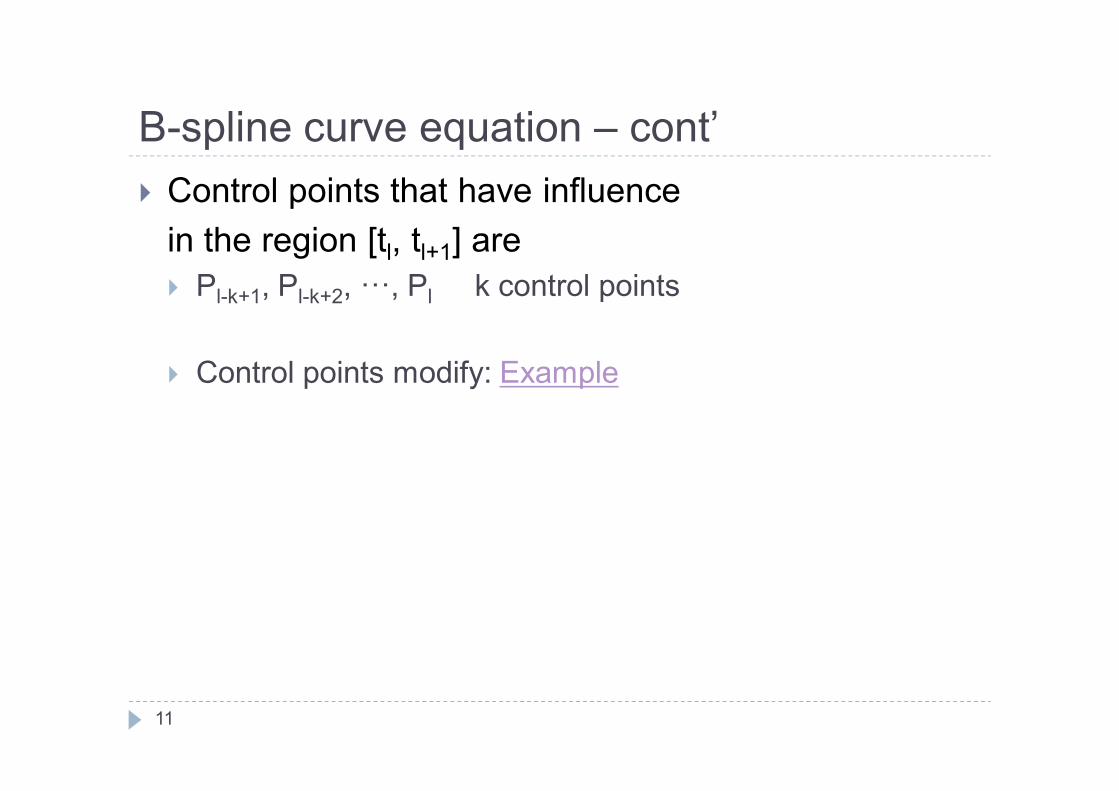
B-spline curve equation – cont’ Control points that have influence
in the region [tl, tl+1] are Pl-k+1, Pl-k+2, ···, Pl k control points
Control points modify: Example
11

B-spline curve - Knot Knot: t0, t1, ···, tn+k
Parameter range is determined by knots Periodic knots
ti= i-k 0≤ i≤ n+k Non-periodic knots
k times duplicatesknin2k-n
nik1k-ik times duplicateski00
ti
12
(d)

Periodic vs. Non-periodic
Periodic knot
Non-periodic knot
13

B-spline curve - Knot By duplicating knot k times at the ends Curve passes through first control point and last control
point Periodic knot First control point and last control point do not pass
through curve as other control points Non-periodic knots are used in most CAD systems
knot interval is uniform in (d) Uniform B-spline (vs. non-uniform B-spline)
During manipulation of curve shape, knots are added or removed Non-uniform knot → non-uniform B-spline curve
14

Example program Knot Insertion Example1
Example2
15
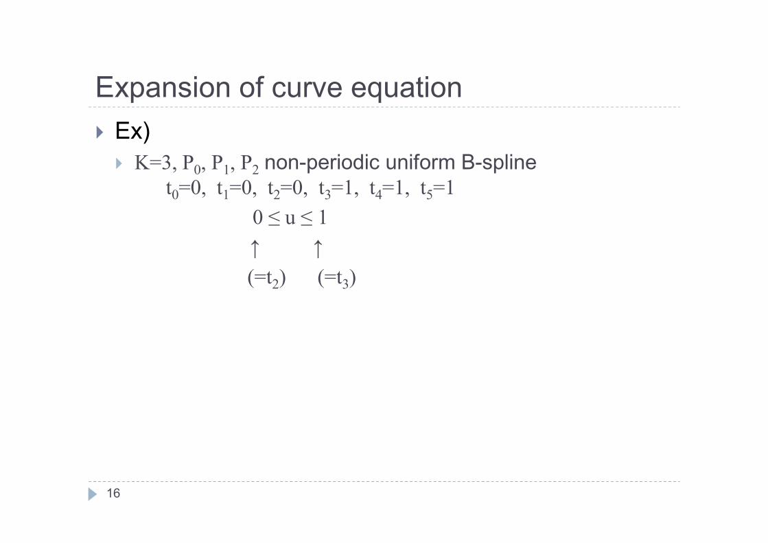
Expansion of curve equation Ex) K=3, P0, P1, P2 non-periodic uniform B-spline
t0=0, t1=0, t2=0, t3=1, t4=1, t5=10 ≤ u ≤ 1↑ ↑(=t2) (=t3)
16

Expansion of curve equation – cont’
17
otherwise01)(utut1
(u)
otherwise01)(utut1
(u)
otherwise01)u(0tut1
(u)
otherwise00)(utut1
(u)
otherwise00)(utut1
(u)
544,1
433,1
322,1
211,1
100,1
N
N
N
N
N

At u=0, select N2,1(u) to be non-zero among N0,1(0), N1,1(0), N2,1(0)
Selection of any one is O.K. At u=1, select N2,1(u) similarly Only N2,1(u) needs to be considered among blending
functions of order 1
Expansion of curve equation – cont’
18

Expansion of curve equation – cont’
192
2
10
2
2
35
3,25
24
2,22
2,3
24
2,24
13
1,21
1,3
21,2
13
1,23
02
0,20
0,3
2,1
34
3,14
23
2,12
2,2
2,1
23
2,13
12
1,11
1,2
uu)-2u(1u)-(1(u)
utt
u)(ttt)t(u(u)
u)2u(1u)u(1u)u(1tt
u)(ttt)t(u(u)
u)(11u)(1
ttu)(t
tt)t(u(u)
u1
utt
u)(ttt)t(u(u)
u)(11u)(1
ttu)(t
tt)t(u(u)
PPPP
NNN
NNN
NNNN
NNNN
NNNN

Consider Bezier curve defined by P0, P1, P2
Non-periodic B-spline curve having k (order) control points ends in Bezier curve
Bezier curve is a special case of B-spline curve
202
111
020 u)(1u
22
u)(1u12
u)(1u02
(u) PPPP
20
Expansion of curve equation – cont’

Example Ex)
K=3, P0, P1, P2, P3, P4, P5
t0=0, t1=0, t2=0, t3=1, t4=2, t5=3, t6=4, t7=4, t8=40≤u≤4
otherwise 04u3 1
(u)
otherwise 03u2 1
(u)
otherwise 02u1 1
(u)
otherwise 01u0 1
(u)
5,1
4,1
3,1
2,1
N
N
N
N
21

22
5,1
67
6,17
56
5,15
5,2
5.14,1
56
5,16
45
4,14
4,2
4.13,1
45
4,15
34
3,13
3,2
3,12,1
34
3,14
23
2,12
2,2
2,1
23
2,13
12
1,11
1,2
3)(utt
u)(ttt)t(u(u)
u)(42)(utt
u)(ttt)t(u(u)
u)(31)(utt
u)(ttt)t(u(u)
u)(2utt
u)(ttt)t(u(u)
u)(1tt
u)(ttt)t(u(u)
NNNN
NNNNN
NNNNN
NNNNN
NNNN
Example – cont’

2,21,224
2,24
13
1,211,3
2,121,213
1,23
02
0,2o0,3
2u2u
ttu)(t
tt)t(u(u)
u)(1u)(1tt
u)(ttt
tuu
NNNNN
NNNNN
3.1
2
2,1 2u)-(2+
2u)u-(2+u)-u(1= NN
3,22,235
3,25
24
2,222,3
2u3
2u
ttu)(t
tt)t(u(u) NNNNN
4,12
3,12,12
2u)(3
21)u)(u(3
2u)u(2
2u NNN
4,23,246
4,26
35
3,233,3
2u4
21u
ttu)(t
tt)t(u(u) NNNNN
5,1
2
4,13,1
2
2u)-(4+
22)-u)(u-(4+
2u)-1)(3-(u+
21)-(u= NNN
23
Example – cont’

5,24,2
57
5,27
46
4,24
4,3 u)(42
2utt
u)(ttt)t(u(u) NNNNN
5,14,1
2
3)u)(u(42
u)2)(4(u2
2)(u NN
5,12
5,2
68
6,28
57
5,25
5,3 3)(u3)(utt
u)(ttt)t(u(u) NNNNN
24
Example – cont’

25
Example – cont’
55,12
45,14,1
2
35,1
2
4,13,1
2
24,1
2
3,12,1
2
3)(u
3)u)(u(42
u)2)(4(u2
2)(u2u)(4
22)u)(u(4
2u)1)(3(u
21)(u
2u)(3
21)u)(u(3
2u)u(2
2u
P
P
P
P
N
NN
NNN
NNN
13,1
2
2,102,12
2u)(2
2u)u(2u)u(1u)(1(u) PPP
NNN

u1 2 3 4
1N0,3 :
u1 2 3 4
1N1,3 :
u1 2 3 4
1N2,3 :
u1 2 3 4
1N3,3 :
1 2 3 4
1
u
N4,3 :
1 2 3 4
1
u
N5,3 :
26
Example – cont’

For each knot interval, coefficients of certain control points = 0 Only subset of control points has influence
For 0≤u≤1, all Ni,1 except N2,1 are 0
27
Example – cont’
2
2
102
1
2u
2u)u(2u)u(1u)(1(u) PPPP

Similarly
Example – cont’
52
42
3
2
4
4
2
32
2
2
3
3
2
21
2
2
3)(u32)20u3u(21
2u)(4(u)
4u3
22)(u11)10u2u(
21
2u)(3(u)
3u2
21)(u
21)u)(u(3
2u)u(2
2u)(2(u)
2u1
PPPP
PPPP
PPPP
28

29
Example – cont’
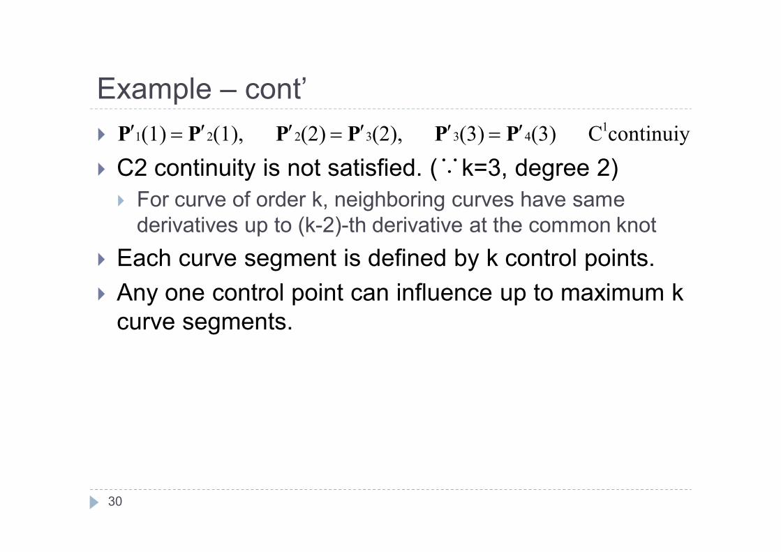
C2 continuity is not satisfied. (∵k=3, degree 2) For curve of order k, neighboring curves have same
derivatives up to (k-2)-th derivative at the common knot Each curve segment is defined by k control points. Any one control point can influence up to maximum k
curve segments.
Example – cont’
30
continuiyC(3)(3)(2),(2)(1),(1) 1433221 PPPPPP

count curve segment including Pk-1
P0 P1 Pk-1 Pk Pn-k Pn-k+1 Pn-1 Pn
P1( )u
P2 ( )u
Pn-k+1( )u
Pn-k+2 ( )u
31
Example – cont’

Least squares curve approximation (Interpolation)
Determine parameter values corresponding to data points
k=1,…,m-1
32

Calculation of control points
mn00
i
QPQP
P )C(
,
]1,0[)(Ni
uuun
0i
m)thansmallerisn(
)(minimizing PPfor Look 2
1-n1
1-m
1k kkuf CQ
33
Least squares curve approximation – cont’

Least squares curve approximation – cont’
34

Least squares curve approximation – cont’
1n2,1,lf
l
,forminimumat0 P
35

Least squares curve approximation – cont’ One equation with n variables P1 ……, Pn-1. l can be 1, ……, n-1 n-1 equations with n-1 variables can be can be generated
(NTN) P = R
36
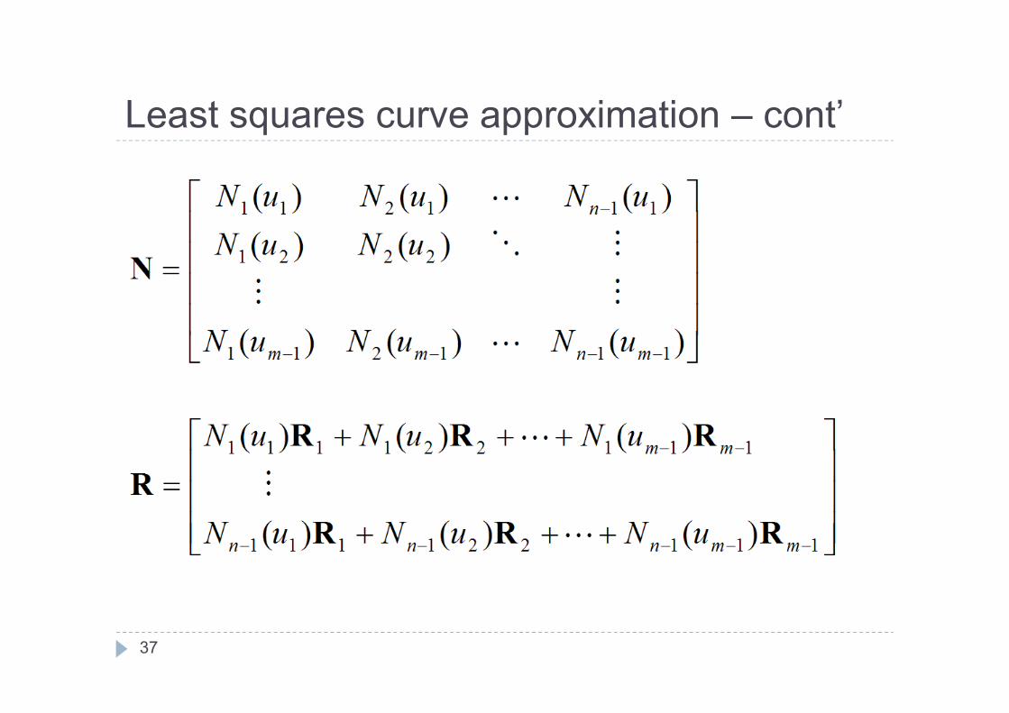
Least squares curve approximation – cont’
37

Least squares curve approximation – cont’ Determination of Knot vector (n+k+1) knots are needed for order k (n-k+1) internal knots need to be determined since k
multiple knots at 0, 0, … , 0 and 1,1, … ,1 already exist
38

Least squares curve approximation – cont’
jqii satisfyinginteger highest theis
39
Internal knots

Least squares curve approximation – cont’Example 1
5.3244
16,644
When
qmkn
For j = 1
40
Knot vector = {0,0,0,0,t4,1,1,1,1}
i=int(1·3.5)=3α=1·3.5-3=0.5T4-1+1= t4 =(1-0.5)u3-1+0.5u3
=0.5(u2+u3)

Least squares curve approximation – cont’
313
245112
,1245
When
q
mkn
41
Example 2

Least squares curve approximation – cont’
42

P(u) – Q(v) = 0 3 scalar equations, two unknowns Px(u) – Qx(v) = 0 Py(u) – Qy(v) = 0
Use Newton Raphson method Derivative of Px, Qx, Py, Qy need to be calculated f1(x1,…,xn) = 0
f2(x1,…,xn) = 0
fn(x1,…,xn) = 0
43
Intersection between curves

n
2
1
n
2
1
n
n
1
n
n
2
1
2
n
1
1
1
nn
n1
1
nn1nnn2211n
nn
11
1
1n11nn22111
f
f
f
xΔ
xΔ
xΔ
xf
xf
xf
xf
xf
xf
xΔxfxΔ
xf)x,,(xf)xΔx,,xΔx,xΔ(xf
xΔxfxΔ
xf)x,,(xf)xΔx,,xΔx,xΔ(xf
44
Intersection between curves – cont’

Intersection between curves – cont’ If initial values of u, v are too far from real solution, the
iteration diverges. Hard to find all the intersection points. Cannot handle the case of overlapping curves. Two curves are regarded to intersect each other if they lie
within numerical tolerance. Control polygons are approximated to the curve by
subdivision and initial values of u,v can be provided closely by intersecting control polygons
Better to detect special situation in advance before resorting to numerical solution.
Tuning tolerance values is necessary
45

Straight line vs. curve P(u) = P0 + u(P1 – P0) Q(v) = P0 + u(P1 – P0) (a) Apply dot product (P0×P1) to both sides of eq(a) gives
(P0×P1)·Q(v) = 0non-linear equation of v
46

Non-uniform Rational B-spline (NURBS) curve Use same Blending functions as B-spline Control points are given in homogeneous
coordinates
n
ikii
n
ikiii
n
ikiii
n
ikiii
iiiiiiiiii
uNhh
uNzhhz
uNyhhy
uNxhhx
hhzhyhxzyx
0,
0
,
0,
0,
)(
)()(
)()(
)()(
),,,(),,(
47

Non-uniform Rational B-spline (NURBS) curve – cont’
)(
)()(
0
,
0
,
n
ikii
n
ikiii
uNh
uNhu
Passes through the 1st and the last control points
( When non-periodic knots are used )
Numerator is B-spline with hiPi as control points
→ h0P0, hnPn at parameter boundary values
Similarly denominator has values of h0, hn at parameter boundary values
48

Non-uniform Rational B-spline (NURBS) curve – cont’
1)(1 ,
0
splineBuNh ki
n
ii
Directions of tangent vectors are P1-P0, Pn-Pn-1 at starting and ending points
B-spline curve is a special case of NURBS
49

Non-uniform Rational B-spline (NURBS) curve – cont’ Curve shape can be changed by changing weight(hi) Increasing weight has an effect of pulling curve
toward associated control point Example program
Conic curve can be represented exactly Reducing program coding effort
50

Control points of NURBS curve equivalent to a circular arc
Can be used when center angle is less than 180o.
Arc with a center angle bigger than 180o is split into two and combined later
51
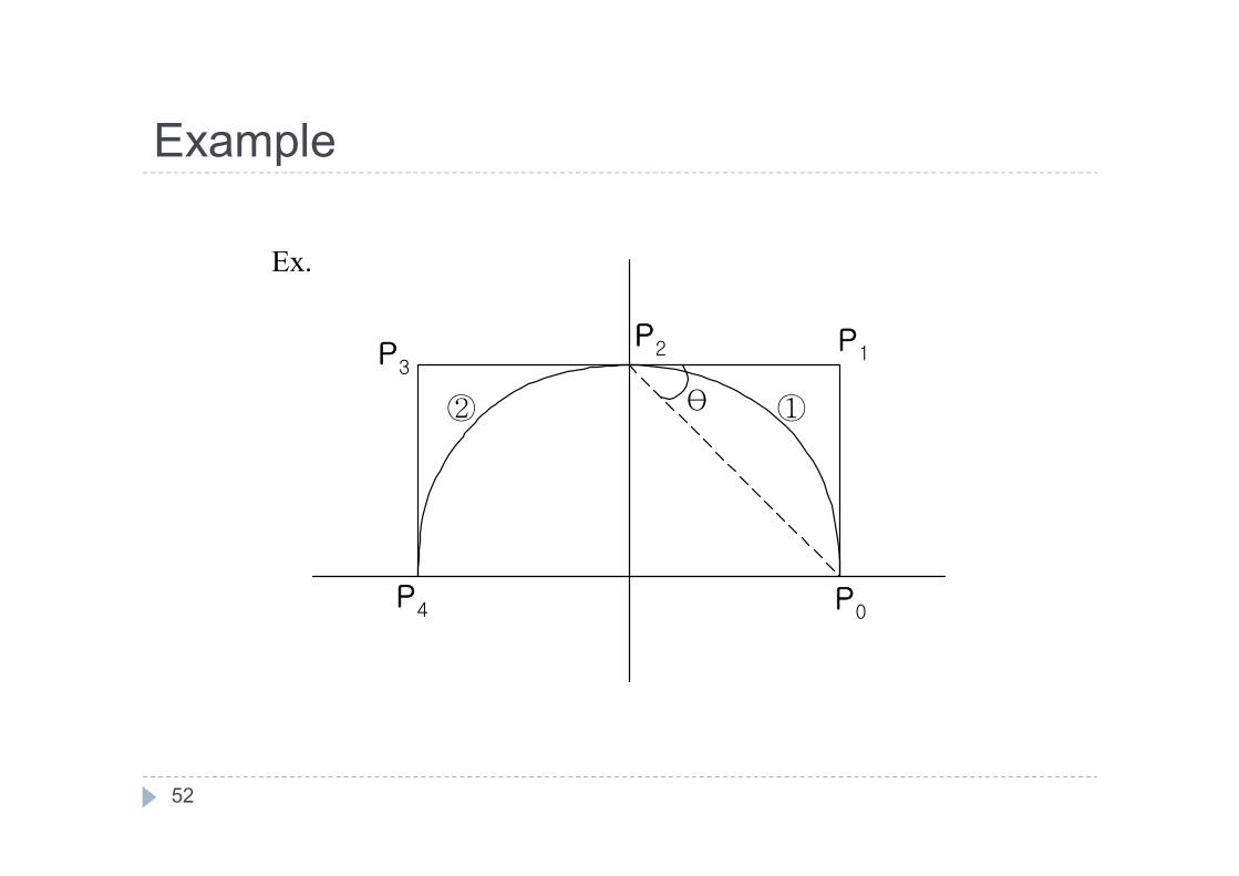
Example
Ex.
P2 P1
P0P4
P3
θ ①②
52

Example – cont’
222111111000
1,2
1,1
)0,1(),1,1(),1,0(
)3,2(111000
12
145cos1
)1,0(),1,1(),0,1(
432
432
210
210
knot
hhh
knknot
hhh
Similarly,
53

Example – cont’
22211000
1,2
1
12
11
)0,1(),1,1(),1,0(),1,1(),0,1(
합성
43
210
43
210
knot
hh
hhh
Composition
54


