76
UNIVERSIDAD AUTONOMA DE MADRID ESCUELA POLITECNICA SUPERIOR PROYECTO FIN DE CARRERA Vibration Isolation with Skyhook Damping Pablo Wildschut Septiembre 2013

UNIVERSIDAD AUTONOMA DE MADRID
ESCUELA POLITECNICA SUPERIOR
PROYECTO FIN DE CARRERA
Vibration Isolation with Skyhook Damping
Pablo Wildschut
Septiembre 2013

1
Vibration Isolation with Skyhook Damping
AUTOR: Pablo Wildschut
TUTOR: Siep Weiland
Dpto. de Tecnología Electrónica y de las Comunicaciones
Escuela Politécnica Superior
Universidad Autónoma de Madrid
Septiembre de 2013

2
Contents
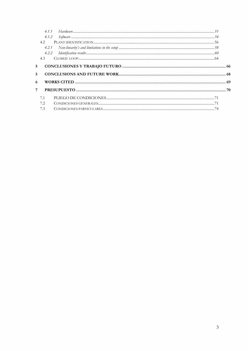
RESUMEN ........................................................................................................................................................... 6
ABSTRACT .......................................................................................................................................................... 7
1 INTRODUCCIÓN ...................................................................................................................................... 8
1.1 MOTIVACIÓN ........................................................................................................................................................... 8 1.2 OBJETIVOS ............................................................................................................................................................... 8 1.3 CONTENIDOS DE LOS APARTADOS ...................................................................................................................... 9
1 INTRODUCTION ..................................................................................................................................... 10
1.1 MOTIVATION ......................................................................................................................................................... 10 1.2 OBJECTIVES............................................................................................................................................................ 10 1.3 CHAPTER CONTENTS ............................................................................................................................................ 11
2 STATE OF THE ART ................................................................................................................................ 12
2.1 LITHOGRAPHIC MACHINES ................................................................................................................................. 12 2.2 METROFRAME........................................................................................................................................................ 13 2.3 ISOLATION OF THE METROFRAME ..................................................................................................................... 13
2.3.1 Passive isolation .................................................................................................................................................... 16 2.3.2 Active isolation ..................................................................................................................................................... 18
2.4 PLANT UNCERTAINTIES AND ROBUSTNESS ...................................................................................................... 19
3 CONTROL DESIGN METHOD’S STUDY .............................................................................................. 21
3.1 INTRODUCTION ..................................................................................................................................................... 21 3.1.1 Simulation models ................................................................................................................................................ 21 3.1.2 Control system ...................................................................................................................................................... 24 3.1.3 Performance requirements ...................................................................................................................................... 24 3.1.4 Generic filter description ........................................................................................................................................ 25
3.2 METHOD 1: CLASSICAL LOOPSHAPING DESIGN .............................................................................................. 26 3.2.1 Acceleration loop design ........................................................................................................................................ 27 3.2.2 Position loop design ............................................................................................................................................... 29 3.2.3 Full controller stability analysis ............................................................................................................................. 30 3.2.4 Controller’s Results ............................................................................................................................................... 32 3.2.5 Conclusions ........................................................................................................................................................... 33
3.3 H-INFINITY THEORY ............................................................................................................................................ 33 3.3.1 H-infinity norm .................................................................................................................................................... 34 3.3.2 H-infinity design algorithms .................................................................................................................................. 34 3.3.3 Augmented plant .................................................................................................................................................. 34 3.3.4 Controllability and observability............................................................................................................................ 36 3.3.5 Robust stability analysis. ...................................................................................................................................... 37
3.4 METHOD 2: MINIMIZATION OF METROFRAME‟S MOVEMENT DESIGN ....................................................... 39 3.4.1 Weights used......................................................................................................................................................... 40 3.4.2 Results .................................................................................................................................................................. 41 3.4.3 Conclusions ........................................................................................................................................................... 43
3.5 METHOD 3: SHAPING WITH DESIRED COMPLIANCE AND TRANSMISSIBILITY DESIGN ............................. 43 3.5.1 Desired transmissibility and compliance ................................................................................................................ 45 3.5.2 Weights used......................................................................................................................................................... 45 3.5.3 Results .................................................................................................................................................................. 47 3.5.4 Conclusions ........................................................................................................................................................... 50
3.6 CONCLUSIONS ....................................................................................................................................................... 50
4 REAL TIME IMPLEMENTATION ......................................................................................................... 51
4.1 TEST SETUP ............................................................................................................................................................ 51
3
4.1.1 Hardware ............................................................................................................................................................. 51 4.1.2 Software ............................................................................................................................................................... 54
4.2 PLANT IDENTIFICATION ...................................................................................................................................... 56 4.2.1 Non-linearity’s and limitations in the setup .......................................................................................................... 58 4.2.2 Identification results .............................................................................................................................................. 60
4.3 CLOSED LOOP ....................................................................................................................................................... 64
5 CONCLUSIONES Y TRABAJO FUTURO .............................................................................................. 66
5 CONCLUSIONS AND FUTURE WORK ................................................................................................. 68
6 WORKS CITED ......................................................................................................................................... 69
7 PRESUPUESTO ........................................................................................................................................ 70
7.1 PLIEGO DE CONDICIONES ........................................................................................................................ 71 7.2 CONDICIONES GENERALES ................................................................................................................................. 71 7.3 CONDICIONES PARTICULARES ............................................................................................................................ 74

4
Table of figures Figure 2-1 - ASML Lithographic machine schema 12 Figure 2-2 - Airmounts position and coordinate system of the metroframe 13 Figure 2-3 - Transmissibility and compliance of a mass-spring damper model 14 Figure 2-4 - Mass-Spring-Damper schematic representation 14 Figure 2-5 - Isolation improvements on transmissibility 15 Figure 2-6 - Isolation improvements on compliance 16 Figure 2-7 - Effect of different stiffness’s of the springs in the transmissibility and compliance. 17 Figure 2-8 - Effect of different damping’s to transmissibility and compliance. 18 Figure 2-9 - Typical feedback control configuration for plant and controller 18
Figure 3-1 - Mass-Spring-Damper schematic representation 21 Figure 3-2 - Alternative block schematic on the 1DoF model 22 Figure 3-3 - Block schematic of the 1DoF model 22 Figure 3-4 – Transfer functions from the mass-spring-damper model. 24 Figure 3-5 - Classic closed loop configuration of plant and controller 24 Figure 3-6 - Filter example 25 Figure 3-7 - Bode plot of Controller’s freq. response 27 Figure 3-8 - Plants acceleration and speed open loop transfer functions. 28 Figure 3-9 - Open Loop Nyquist plot. 28 Figure 3-10 - Open Loop diagram of the transmissibility with the acceleration controller. 28 Figure 3-11 - Open Loop Bode and Nyquist plot with only the integral as controller. 29 Figure 3-12 - Open Loop Bode and Nyquist plot. 30 Figure 3-13 - Full controller open loop configuration. 30 Figure 3-14 - Full controller open loop Bode plot. 31 Figure 3-15 - Open Loop Nyquist plot. 32 Figure 3-16 - Noise-Displacement frequency bode plots 32 Figure 3-17 - Transmissibility and compliance of the classic loopshaping method controller 33 Figure 3-18 - H-infinity plant plus controller configuration 34 Figure 3-19 - Augmented plant scheme 34 Figure 3-20 - Augmented plant setup for simplified example 35 Figure 3-21 - Augmented plat’s open Loop and H-infinity controller’s closed loop comparison. 36 Figure 3-22 - Example of allowable uncertainty in a SISO system 38 Figure 3-23 - Uncertainties in the LFT configuration. 38 Figure 3-24 - Augmented plant for minimization of the metroframe 39 Figure 3-25 - Effect of evening out compliance´s -2 slope 40 Figure 3-26 - Obtained transmissibility and compliance for the minimization of position approach 41 Figure 3-27 - Open loop for the minimization of position approach 41 Figure 3-28 – Structured uncertainty limit for each input and output of the system. 42 Figure 3-29 - Unstructured uncertainty limit of the system 43 Figure 3-30 - Augmented plant for the shaping desired transfers method. 44 Figure 3-31 - Desired transmissibility and compliance 45 Figure 3-32 - Absolute difference versus logarithmic difference in bode plot. 46 Figure 3-33 - Transmissibility and Compliance from the desired plant approach 47 Figure 3-34 - Open loop for the desired transfers approach. 47 Figure 3-35 - Transmissibility and compliance with alternative desired transfers 48 Figure 3-36 - Structured uncertainty limit for each input and output of the system. 49 Figure 3-37 - Unstructure uncertainty limit for the controlled system. 50

5
Figure 4-1 –Directions of Lorentz actuators and position sensors in the metroframe in the horizontal
plane. 51 Figure 4-2 - Connections within the test setup 52 Figure 4-3 - Accelerometer and signal conditioner 53 Figure 4-4 - Input and output board of the dSpace system 53 Figure 4-5 - Stateflow chart for the initialization of the system 54 Figure 4-6 - Pneumatic controllers on the Simulink model 55 Figure 4-7 - Lorentz controller blocks on the Simulink model 56 Figure 4-8 – Gaussian noise added to the closed loop within the dspace environment 57 Figure 4-9 - Process used to obtain cleaner frequency responses from measured data 58 Figure 4-10 - Results from high frequency pole elimination in H-infinity controllers 60 Figure 4-11 - Measured plant frequency response from Force to Position 61 Figure 4-12 - Measured plant frequency response from force to acceleration 62 Figure 4-13 - Modelled vs identified plant frequency response magnitude 63 Figure 4-14 - Modelled vs identified plant frequency response phase 64 Figure 4-15 - Manually tuned controller closed loop. 65

6
Resumen Este proyecto se centra en estudiar diferentes métodos de diseño de controladores y en crear
un método de diseño adecuado para un sistema de aislamiento activo. La necesidad en un
método distinto a los actuales se debe al aumento de la complejidad en el tuneado de los
controladores con los métodos clásicos de diseño cuando se tienen dos o más lazos cerrados y
a que se está tratando de añadir un lazo adicional a los sistemas de aislamiento mediante
acelerómetros. Se hace uso del método H-infinito debido a la posibilidad de este de obtener
controladores óptimos sin ser afectado por la complejidad de la planta. El problema de los
métodos H-infinito es que el tuneado es difícil de comprender y dominar. Durante el estudio
de distintos métodos se ha obtenido una versión de un método H-infinito que es capaz de
obtener controladores con un proceso de tuneado que es más fácil de comprender. Este
método hace uso de la respuesta en frecuencia deseada para el sistema para obtener el
controlador óptimo.
Se ha visto además que aunque en la simulación los resultados en aislamiento obtenido por los
controladores sean aceptables una vez aplicado a una máquina física estos no son aceptables.
Esto se debe a que es necesario estudiar la máquina física para añadir al tuneado del
controlador información sobre incertidumbres para garantizar robustez en la estabilidad o en
el rendimiento del controlador.

7
Abstract This project is centred to study different control design methods and create a suitable design
method for an active isolation system. The study is pushed by the increased complexity in
tuning controllers with classical methods for controllers with two or more loops. The H-
infinity method is chosen due to the possibility to obtain optimal controllers without being
affected by the complexity of the plant. The problem of H-infinity methods is that its tuning
process is difficult to understand and master. A version of an H-infinity method is obtained
that is able to obtain suitable controllers with a tuning process that has the intuitiveness of
classical methods. This method makes use of the desired output of the controlled system to
obtain the optimal controller to do so.
Two other methods are used to be compared, a classical loopshaping method and a
straightforward approach to the H-infinity methods. The controllers obtained through all
three methods are put to the test in a physical machine. The results are unsuccessful. This
result in comparison with the simulated tests is due to the small stability margins obtained
through the H-infinity method. The conclusion to this work is that in simulated environments
the new method is viable while for physical environments there is a need to add uncertainty
data to the tuning process.
8
1 Introducción
1.1 Motivación Hoy en día se invierte mucho esfuerzo en mejorar los procesos de fabricación de
semiconductores. El motivo es la demanda del mercado en obtener chips de mayor densidad
que sean más rápidos, baratos y eficientes. La velocidad a la que se producen estas mejoras
está descrita por la ley de Moore. Pero a diferencia de las leyes físicas la ley de Moore no es
estricta y es más bien una guía que estima el futuro avance de la tecnología de
semiconductores.
El proceso de fabricación se divide en cuatro etapas principales: Deposición, Litografía,
Ataque químico y alteración de las propiedades eléctricas. En la etapa de litografía es donde el
diseño del chip a fabricar se imprime sobre las obleas de silicio. Hoy en día esta etapa supone
el cuello de botella para la máxima densidad posible en el chip.
ASML produce máquinas de fotolitografía para la industria de semiconductores. Estas
máquinas fotolitográficas están diseñadas para ser capaces de exponer las obleas para obtener
conexiones que se encuentran en órdenes de magnitud entorno a los 20 nanómetros en
anchura. A estas escalas las máquinas son extremadamente sensibles a las vibraciones. Con el
fin de aislar lo más posible de vibraciones y así poder aumentar al máximo el rendimiento de
las máquinas se ha creado un sistema de aislamiento activo de vibraciones.
Hasta hace poco el control del aislamiento activo se hacía a través de un solo sensor. Un
sensor de posición que ofrecía datos sobre la posición relativa al suelo. Obtener datos de
posición relativos limita el máximo grado de aislamiento que se puede conseguir. Por tanto
para superar estas limitaciones es necesario incorporar medidas de posición absolutas. El
aislamiento mediante medidas absolutas es conocido como “Skyhook Damping”. En el
mundo físico no es posible obtener la posición de un objeto sin un punto de referencia pero el
movimiento del objeto (velocidad y aceleración) si es una medida absoluta y está relacionada
con la posición.
El mercado de los acelerómetros ha llegado a un punto donde es factible hacer uso de estos
sensores para detectar las mínimas aceleraciones que se buscan controlar en las máquinas
litográficas.
Sin embargo añadir un segundo tipo de medidas a un sistema de control aumenta la dificultad
en la creación de un controlador capaz de optimizar el aislamiento mediante los métodos
clásicos de control. Por tanto es necesario investigar la posibilidad de obtener un controlador
para sistemas de control más complejos. La opción que se probará en este proyecto es el de
los métodos H-infinito.
1.2 Objetivos El objetivo principal del proyecto será el de obtener un método para crear un controlador para
un sistema con dos lazos cerrados, uno por un sensor de posición relativo y otro por un
acelerómetro mediante métodos de H-infinito.
9
El problema con los métodos H-infinito es que el proceso de tuneado consume tiempo y es
muy poco intuitivo. Por lo tanto el objetivo de este proyecto es el de crear un método de
diseño del controlador mediante H-infinito que haga el tuneado más sencillo y comparar sus
resultados con otros métodos más comunes. Los pasos a seguir serán los siguientes:
• Diseño de un controlador con el método loopshaping clásico.
• Diseño de un controlador con un método H-infinito sencillo muy utilizado en la
literatura.
• Diseño de un controlador usando un método H-infinito modificado para ser más
intuitivo.
• Prueba de los tres controladores en un entorno real para demostrar sus capacidades y
comparar los resultados de los controladores obtenidos a través de los diferentes
métodos.
1.3 Contenidos de los apartados
El Capítulo 2 proporcionará conceptos que se utilizarán como base para el proyecto.
También mostrará el estado del arte en los sistemas de aislamiento activo y los métodos de
diseño de control para sistemas de aislamiento.
El Capítulo 3 mostrará el proceso de tuneado de los tres métodos de diseño de control
utilizados. También se muestran los resultados de los controladores obtenidos y una
comparación entre ellos.
El Capítulo 4 mostrará el sistema de test creado y los resultados obtenidos.
El Capítulo 5 son las conclusiones finales del proyecto.

10
1 Introduction
1.1 Motivation
There is a lot of research effort being put onto the improvements in manufacturing processes
of semiconductor devices nowadays. The reason is the demand of the market to be able to
produce higher density chips which are faster, more efficient and cheaper. The rate at which
these improvements occur is known as the Moore´s law. But unlike scientific laws Moore´s is
not a strict one and there is a lot of research effort needed to improve the manufacturing
process of chips in order to be able to keep obeying this law.
The manufacturing process can be divided into four main stages: deposition, patterning,
removal and modification of electrical properties. It is in the patterning stage where the layout
of the manufactured chip is printed onto the wafers. Nowadays this stage is a bottleneck for
the maximum density of the chips.
ASML creates photolithographic machines which will print the desired pattern onto the
wafers that contain the chips. These photolithographic machines are designed to be able to
expose the wafers to create lines that are in the orders of the 20 nanometers in width. These
machines are therefore extremely sensitive to vibrations. In order to prevent these vibrations
from affecting the machines performance an isolation system is created.
Until recently the active method for vibration isolation that has been used in ASML was based
on position sensors. These position sensors give readings of the distance between the ground
and the isolated surface which are known as referential readings. With referential readings
there is a limitation that affects the damping the isolation system can create. To overcome
these limitations another sensor has been added to the isolation system, an accelerometer.
Accelerometers give absolute readings. With absolute readings a different type of damping can
be created that is called Skyhook damping.
1.2 Objectives
Designing controllers to act in accordance with the readings of several sensors with the
classical loopshaping methods is challenging. As the number of control loops increases the
number of variables to take into consideration also increases making achieving a good
performance harder to obtain. To be able to overcome this problem a different controller
design method has to be used. This method will be the H-infinity loopshaping method that is
capable of achieving optimal controllers for any number of parallel control loops.
The problem with the H-infinity methods is that the tuning process is time consuming and
very unintuitive. Therefore the focus of this project will be that of creating a controller design
method using H-infinity that will make the tuning process easier. The steps will be as follow:
Designing a controller with the classical loopshaping method
Designing a controller with a straightforward H-infinity method as seen in several
research papers
Designing a controller using a modified H-infinity method with a simpler tuning
process.

11
Testing all three controllers in a real environment to prove their capacities and
compare the results of the controllers obtained through the different methods.
1.3 Chapter contents
Chapter 2 will provide concepts that will be used as the background for the project. It will
also show state of the art on active isolation and isolation control design methods.
Chapter 3 will show the tuning process of the three different control design methods. It will
also show the results of the obtained controllers and a comparison between the methods
Chapter 4 will show the test setup created and the results obtained with it.
Chapter 5 contains the final conclusions of the project
12
2 State of the art
2.1 Lithographic machines
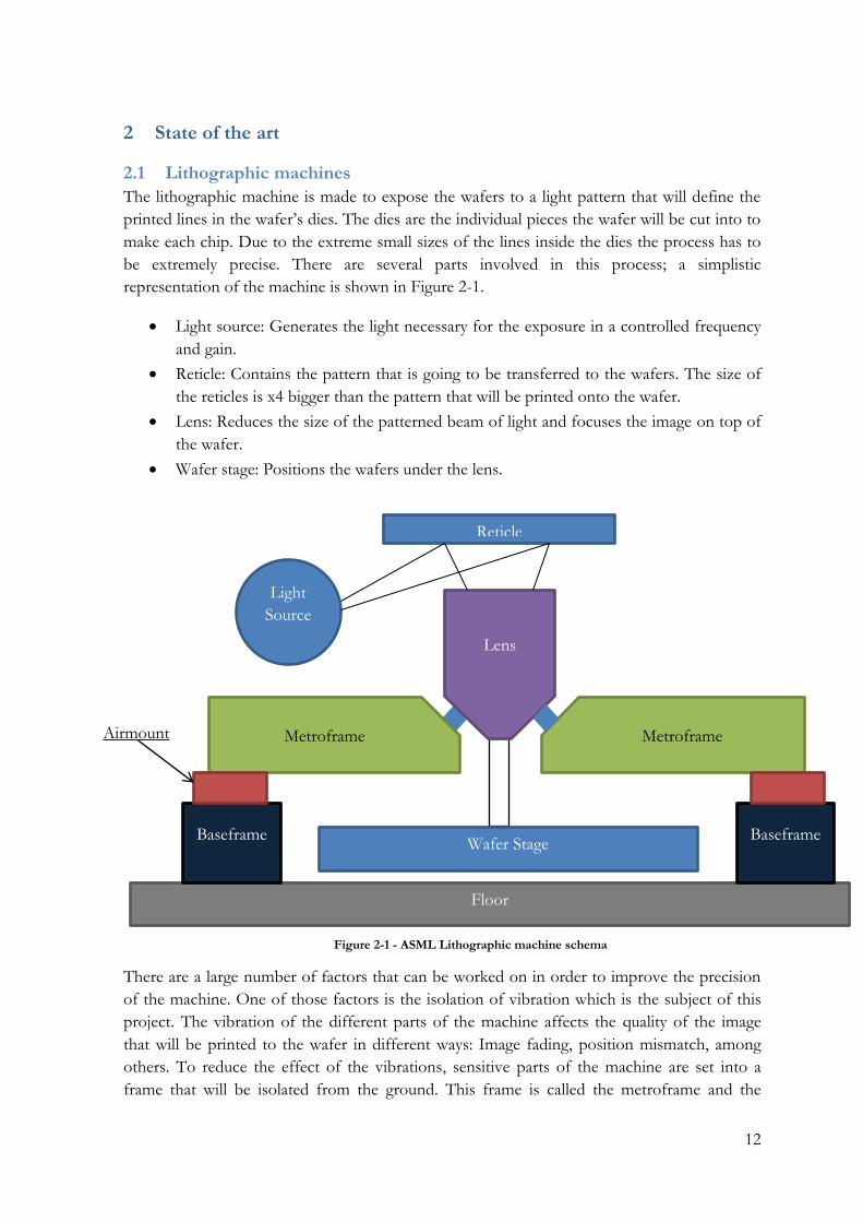
The lithographic machine is made to expose the wafers to a light pattern that will define the
printed lines in the wafer‟s dies. The dies are the individual pieces the wafer will be cut into to
make each chip. Due to the extreme small sizes of the lines inside the dies the process has to
be extremely precise. There are several parts involved in this process; a simplistic
representation of the machine is shown in Figure 2-1.
Light source: Generates the light necessary for the exposure in a controlled frequency
and gain.
Reticle: Contains the pattern that is going to be transferred to the wafers. The size of
the reticles is x4 bigger than the pattern that will be printed onto the wafer.
Lens: Reduces the size of the patterned beam of light and focuses the image on top of
the wafer.
Wafer stage: Positions the wafers under the lens.
There are a large number of factors that can be worked on in order to improve the precision
of the machine. One of those factors is the isolation of vibration which is the subject of this
project. The vibration of the different parts of the machine affects the quality of the image
that will be printed to the wafer in different ways: Image fading, position mismatch, among
others. To reduce the effect of the vibrations, sensitive parts of the machine are set into a
frame that will be isolated from the ground. This frame is called the metroframe and the
Floor
Baseframe
Metroframe Metroframe
Wafer Stage Baseframe
Lens
Airmount
s
Reticle
Light
Source
Figure 2-1 - ASML Lithographic machine schema

13
isolation of this metroframe will be achieved through the airmounts that are the support on
which the frame lies.
2.2 Metroframe
The metroframe is an isolated mass that gives support to a number of components within the
machine. Using a frame to support all the components makes it easier to handle as all the
vibration control power is focused on keeping just one big mass free of motion.
The metroframe weighs about 2000Kg. It is supported by three mounts (airmounts) which act
as a system of springs and dampers. They also contain active Lorentz actuators to allow for
active control of the movement of the frame.
The location of these airmounts within the metroframe is shown in Figure 2-2. With this
configuration the metroframe is capable of moving in six different degrees, three position
movements (x, y, z) and three rotational movements (χ, ψ, φ). This enables the metroframe to
be able to isolate from disturbances in all possible directions.
2.3 Isolation of the metroframe
x
y Lens
1
3
2
Figure 2-2 - Airmounts position and coordinate system of the metroframe

14
The different types of disturbances the metroframe has to be isolated from can be divided
into two types, disturbances from the ground
and disturbances affecting the metroframe
directly. To describe how these disturbances
affect the metroframe at different frequencies a
frequency response diagram will be used. Due
to the importance of these frequency responses
they will be called transmissibility and
compliance. In order to understand what kind
of information can be obtained from these plots
a simple 1 DOF model as shown in Figure 2-4
will be used to explain them.
Transmissibility is the transfer function from the position of the base to the position of the
metroframe. If the base movement is „XBF‟ and the position of the metroframe is „XMF‟
transmissibility would be described as
. (see Figure 2-3)
For low frequencies transmissibility starts at 0dB this means that for low frequencies the
metroframe will move with the base maintaining the same relative distance between them.
After the resonance there is a decoupling of the mass from the ground movement that can be
appreciated in the slope. This decrease in magnitude means that the high frequencies of the
vibrations are not being fully transmitted to the metroframe. Due to the existence of a damper
between the ground and the metroframe the magnitude of the resonance peak is reduced.
However it is also a source of vibration transmission to the metroframe, this can be seen in
k
m
b
FMF
XBF
Figure 2-4 - Mass-Spring-Damper schematic representation
XMF
-150
-100
-50
0
50
From: XBF
To: X
MF
10-1
100
101
102
-180
-135
-90
-45
0
To: X
MF
From: FMF
10-1
100
101
102
Bode Diagram
Frequency (Hz)
Magnitude (
dB
) ; P
hase (
deg)
Figure 2-3 - Transmissibility and compliance of a mass-spring damper model

15
the reduction of the slope‟s decrease from being a -2 (-40dB/decade) slope to being a -1 (-
20dB/decade) slope for higher frequencies.
Compliance is transfer function from the Force acting on the metroframe to the position of
the metroframe. If the force is „FMF‟ and the position of the metroframe is „XMF‟ compliance
would be described as
. The form of the compliance‟s
frequency response has a resemblance to the transmissibility however the meaning of results is
slightly different (see Figure 2-3). The flat line for low frequencies describes the resistance to
force that comes from the springs, thus this line is equal to 1/k (inverse of the spring
constant). The slope after the resonance peak is known as the mass line. This is because this
line represents the slope (1/m*s2) which comes from the formula F = m*a. This means that
for higher frequencies the displacement of the mass is minimized because of the resistance of
the mass to change position quickly.
What is expected to be seen in these transfer functions when the isolation of a mass is
improved complies with the following criteria, also schematically shown in Figure 2-5 and
Figure 2-6
1. Damping of the resonant peak
2. Shifting of the resonant peak to lower frequencies.
3. Faster decoupling of the mass from ground vibrations, equivalent to decreasing the
transmissibility‟s magnitude after the resonant peak.
4. For compliance, reductions in magnitude of the transfer function.
Figure 2-5 - Isolation improvements on transmissibility
10-1
100
101
102
-80
-60
-40
-20
0
20
40
From: XBF
To: XMF
(1)
Magnitu
de (
dB
)
Bode Diagram
Frequency (Hz)
1
3
2

16
2.3.1 Passive isolation
Passive isolation is the isolation that can be obtained by the use of different configurations of
springs and dampers. Therefore the tuning parameters are limited to only the stiffness
coefficient („k‟) of the spring and the damping coefficient („d‟) of the damper. Details on what
can be obtained by changing those parameters are shown below. This is done to show the
limitations of passive isolation.
10-1
100
101
102
-200
-150
-100
-50
From: FMF
To: XMF
(1)
Magnitu
de (
dB
)
Bode Diagram
Frequency (Hz)
Figure 2-6 - Isolation improvements on compliance
1
4
2
17
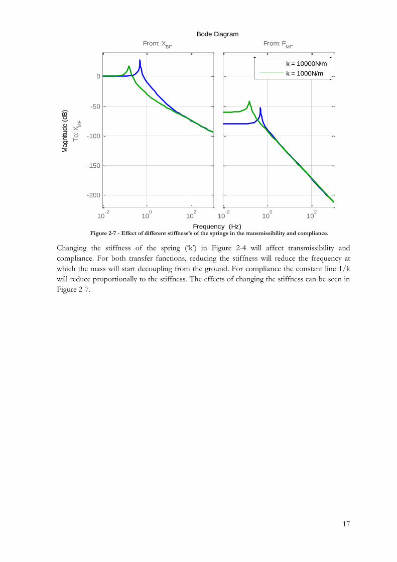
Changing the stiffness of the spring („k‟) in Figure 2-4 will affect transmissibility and
compliance. For both transfer functions, reducing the stiffness will reduce the frequency at
which the mass will start decoupling from the ground. For compliance the constant line 1/k
will reduce proportionally to the stiffness. The effects of changing the stiffness can be seen in
Figure 2-7.
Figure 2-7 - Effect of different stiffness’s of the springs in the transmissibility and compliance.
10-2
100
102
-200
-150
-100
-50
0
From: XBF
To: X
MF
10-2
100
102
From: FMF
Bode Diagram
Frequency (Hz)
Magnitu
de (
dB
)k = 10000N/m
k = 1000N/m
18
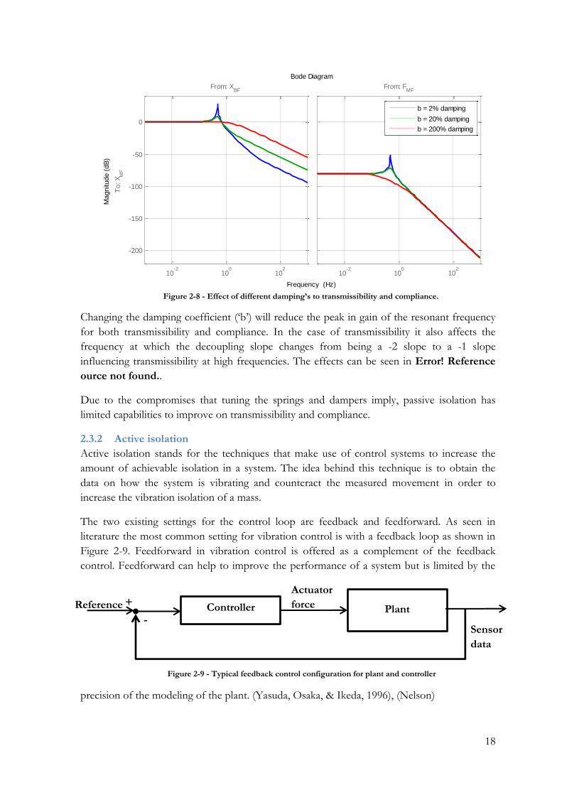
Changing the damping coefficient („b‟) will reduce the peak in gain of the resonant frequency
for both transmissibility and compliance. In the case of transmissibility it also affects the
frequency at which the decoupling slope changes from being a -2 slope to a -1 slope
influencing transmissibility at high frequencies. The effects can be seen in Error! Reference
ource not found..
Due to the compromises that tuning the springs and dampers imply, passive isolation has
limited capabilities to improve on transmissibility and compliance.
2.3.2 Active isolation
Active isolation stands for the techniques that make use of control systems to increase the
amount of achievable isolation in a system. The idea behind this technique is to obtain the
data on how the system is vibrating and counteract the measured movement in order to
increase the vibration isolation of a mass.
The two existing settings for the control loop are feedback and feedforward. As seen in
literature the most common setting for vibration control is with a feedback loop as shown in
Figure 2-9. Feedforward in vibration control is offered as a complement of the feedback
control. Feedforward can help to improve the performance of a system but is limited by the
precision of the modeling of the plant. (Yasuda, Osaka, & Ikeda, 1996), (Nelson)
Controller Plant
Figure 2-9 - Typical feedback control configuration for plant and controller
Reference +
- Sensor
data
Actuator
force
10-2
100
102
-200
-150
-100
-50
0
From: XBF
To: X
MF
10-2
100
102
From: FMF
Bode Diagram
Frequency (Hz)
Magnitu
de (
dB
)b = 2% damping
b = 20% damping
b = 200% damping
Figure 2-8 - Effect of different damping’s to transmissibility and compliance.
19
The main concerns for active vibration control systems are to maintain the stability and the
performance requirements of the system. Being able to do this under uncertain plants (plants
that have imprecise variables or unmodeled parts) is called Robust stability and Robust
performance respectively.
The first methods on vibration control made use of graphical representations to see the
effects of the designed controllers and then use the information to refine its performance.
Usually these graphs were shown in the frequency spectrum and made use of this information
to manipulate the controllers frequency response by adding different types of filters to the
loop. These methods were therefore called as loopshaping methods. (F.Franklin, Powell, &
Emami-Naeini), (C.Doyle, A.Francis, & R.Tannenbaum). These loopshaping methods were
focused on helping the designer to achieve stability while the performance was left to the
designer‟s ability. Robust stability was not ensured but obtained by adding margins to the
stability of the system. A major limitation of these methods is that they are not applicable to
MIMO systems.
As processes to be controlled grew in complexity the industry started to look for methods that
would help to create controllers that could obtain optimality in these multivariable
environments (Skogestad & Postelwaith). One of these methods is known as the H-infinity
synthesis method. This method is able to obtain optimal controllers through the application of
mathematical algorithms. The H-infinity method will be explained later on in 3.3.
The H-infinity method is not a strict method and different ways of making use of these
algorithms have been tried out. For instance, in (Ding C. , Damen, Bosch, & Janssen) a way of
combining H-infinity methods in combination with classical controllers is studied. The
intention is to create a stable system with the classic controller and add a second controller
that would take care of the non-linearity of the system.
There has also been research going on searching for the best configuration of actuators and
sensors to obtain the best performance. In (Wal & Heertjes) different configurations of
sensors were studied it is shown that the combination of relative position sensors and absolute
acceleration gave the best results.
2.4 Plant uncertainties and robustness The plant models created for the simulations are generally not perfect in their representation
of the real plant and the frequency responses differ more or less from one to another. All
these divergences are known as uncertainties. These uncertainties can come from very diverse
causes: unmodeled modes in the plant, resolution limitations of the sensors, non linearities,
etc… To make account of all these different uncertainties they can all be studied as dynamic
uncertainties.
Among the dynamic uncertainties these can be divided into two different types, unstructured
or structured uncertainties. Unstructured are the uncertainties whose origin is unknown or too
disperse and therefore affect the entire system at once. Structured uncertainties are
uncertainties that can be narrowed to only one transfer function within a system and therefore
studied individually.

20
Uncertainties can also be described as to where they are applied within the loop: as input
multiplicative uncertainties, output multiplicative, additive, etc… From now on additive
uncertainty will be used and it is expressed as follows:
PΔ symbolizes all the possible plants that the system tries to describe. P is the ideal plant and
is the uncertainty if the plant. The property of a controller to stabilize all the possible plants is
called robustness.
21
3 Control design method’s study
3.1 Introduction
Three different methods will be used to create a controller for the same plant. The intention is
to be able to afterwards compare the designing process of each of these methods. The
methods to be compared are the following.
1. Method 1 is the classical loopshaping method.
2. Method 2 is a simple approach to the H-infinity method
3. Method 3 intents to simplify the tuning process of the H-infinity method.
For any of the methods to be tried out, some initial specifications need to be set. These
specifications are the model for the simulation environment, the control system structure and
the performance goals to be achieved by the controller.
3.1.1 Simulation models
In order to be able to create a control system for the real plant it is necessary in the first place
to create a suitable simulation model. The model does not need to be a perfect representation
of the real life machine; it actually is beneficial to create a simplified model to make it is easier
to study the effect of the controllers.
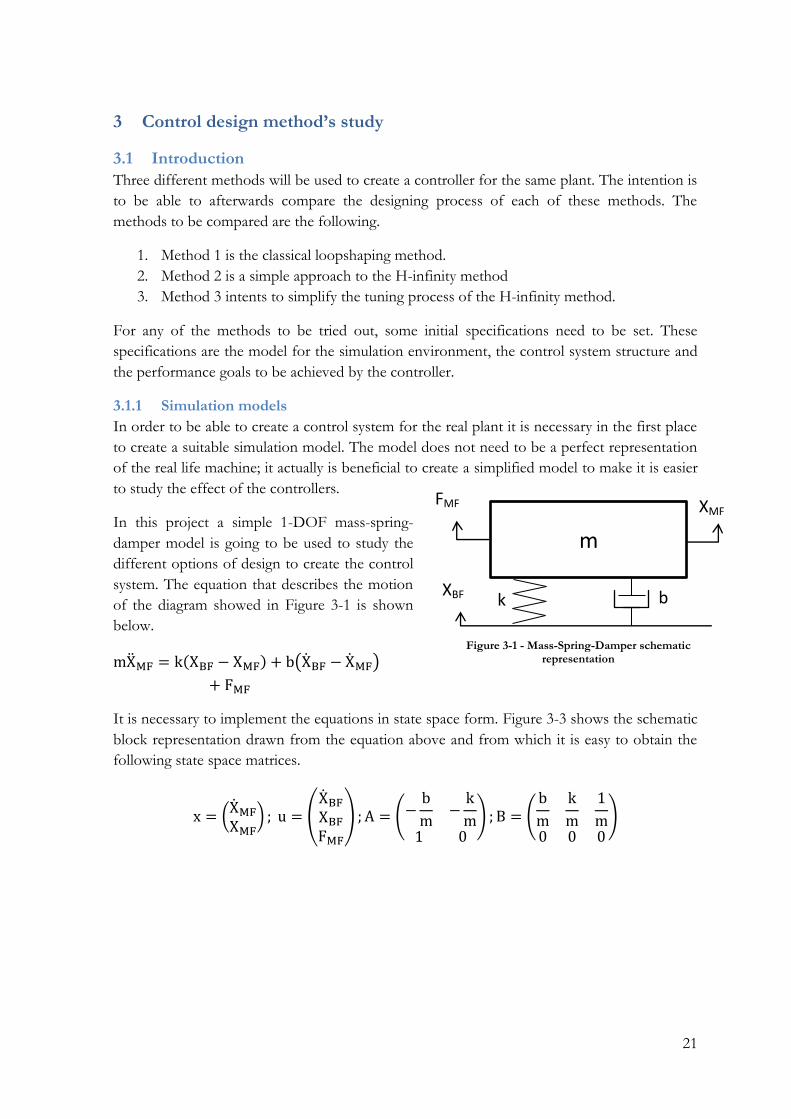
In this project a simple 1-DOF mass-spring-
damper model is going to be used to study the
different options of design to create the control
system. The equation that describes the motion
of the diagram showed in Figure 3-1 is shown
below.
mX k(X − X ) b(X − X )
F
It is necessary to implement the equations in state space form. Figure 3-3 shows the schematic
block representation drawn from the equation above and from which it is easy to obtain the
following state space matrices.
(X X
* (X X F
) (−b
m−k
m
+ (b
m
k
m
m
+
k
m
b
FMF
XBF
Figure 3-1 - Mass-Spring-Damper schematic representation
XMF
22
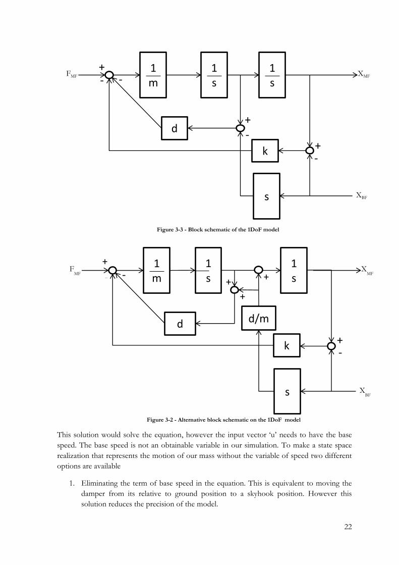
This solution would solve the equation, however the input vector „u‟ needs to have the base
speed. The base speed is not an obtainable variable in our simulation. To make a state space
realization that represents the motion of our mass without the variable of speed two different
options are available
1. Eliminating the term of base speed in the equation. This is equivalent to moving the
damper from its relative to ground position to a skyhook position. However this
solution reduces the precision of the model.
1
m
1
s
1
s
d
s
k
+
+
+
-
-
- -
Figure 3-3 - Block schematic of the 1DoF model
FMF XMF
XBF
1
m
1
s
1
s
d
s
k
+
+
+
-
- -
FMF
XMF
XBF
d/m
+
+
Figure 3-2 - Alternative block schematic on the 1DoF model
23
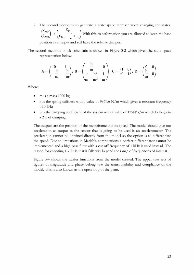
2. The second option is to generate a state space representation changing the states.
(X X
* (X
X −
X
) With this transformation you are allowed to keep the base
position as an input and still have the relative damper.
The second methods block schematic is shown in Figure 3-2 which gives the state space
representation below:
(
−k
m−b
m
+ (
b
m
k
m−b
m
m
, (
) ( b
m +
Where:
m is a mass 1000 kg.
k is the spring stiffness with a value of 9869.6 N/m which gives a resonant frequency
of 0.5Hz
b is the damping coefficient of the system with a value of 125N*s/m which belongs to
a 2% of damping.
The outputs are the position of the metroframe and its speed. The model should give out
acceleration as output as the sensor that is going to be used is an accelerometer. The
acceleration cannot be obtained directly from the model so the option is to differentiate
the speed. Due to limitations in Matlab‟s computations a perfect differentiator cannot be
implemented and a high pass filter with a cut off frequency of 1 kHz is used instead. The
reason for choosing 1 kHz is that it falls way beyond the range of frequencies of interest.
Figure 3-4 shows the trasfer functions from the model created. The upper two sets of
figures of magnitude and phase belong two the transmissibility and compliance of the
model. This is also known as the open loop of the plant.

24
3.1.2 Control system
The controller to be designed will have two inputs, one from the position sensor and another
from an accelerometer. The output of the controller will be force to the actuators that go into
the plant. The systems closed loop diagram is shown below.
3.1.3 Performance requirements
The main goal of the controller is to increase the isolation of a system. Therefore the
requirements on performance are the same as those shown in section 2.4 to improve on
isolation.
Other requirements that will affect the controller‟s design are:
Position (XMF-XBF)
Acceleration (AMF) Controller Plant
Force on metroframe
(FMF) Base Movement
(XBF)
Figure 3-5 - Classic closed loop configuration of plant and controller
Figure 3-4 – Transfer functions from the mass-spring-damper model.
-200
-100
0
From: XBF
To: X
MF
-180
-90
0
To: X
MF
-100
-50
0
50
To: A
MF
10-1
100
101
102
-180
0
180
To: A
MF
From: FMF
10-1
100
101
102
Bode Diagram
Frequency (Hz)
Magnitu
de (
dB
) ; P
hase (
deg)

25
1. Reduction of control gain to minimize the effect of sensor noise
2. Adding robustness to the system by not adding gain to the controller at frequencies
higher than 100 Hz.
3.1.4 Generic filter description
To be able to easily show the structure of a filter a generic description is going to be made.
This generic description is going to be used in the rest of the document. The generic transfer
function F(s) for these filters is shown below:
( ) ∏(
*
∏
(
*
g is the gain of the filter.
Each fi represents the frequency at which a zero is placed in the bode plot.
Each fj represents the frequency at which a pole is placed in the bode plot.
The format at which filters will be shown further on through the document is the following.
Example filter: {
( )
( )
( )
0
10
20
30
40
Magnitu
de (
dB
)
10-1
100
101
102
103
104
-90
-45
0
45
90
Phase (
deg)
Bode Diagram
Frequency (Hz)
Figure 3-6 - Filter example

26
In the case of a double pole or double zero the equation used instead of two single poles or
zeros is:
( ) ((
*
(
* )
((
*
( * )
Where the symbol is the damping coefficient and which would be ½ if not stated otherwise.
3.2 Method 1: Classical loopshaping design
Our controller is made out of two different control loops. This means that two controllers
have to be designed, one for the acceleration loop and another for the position loop. Each
loop has its own characteristics and will be therefore used to fulfill different requirements.
The accelerometer gives absolute readings. This gives the possibility to damp the metroframe
without affecting the transmissibility. For this reason the acceleration loop will be used to
damp the resonant peak. It will also be used as far as possible to damp at frequencies close to
the resonant peak.
The position loop gives relative data, adding gain to this loop has the same effects as
increasing the damping. Therefore adding gain to frequencies over 0.5 Hz must be avoided so
to not affect transmissibility. The position loop will be used to add integral action to the
controller to prevent from low frequency noises that can displace the metroframe.
The design process will be the following:
1. First the acceleration loop will be tuned on performance and stability.
2. Afterwards the position loop.
3. The performance and the stability of both controllers working in parallel will be tested.
If the system is either unstable or the performance is not considered good enough the
steps will be repeated.
4. Noise parameters will be added. The performance on noise cancellation will be
checked, in the case of unsatisfactory results the steps will be repeated.
With this method the best performance is going to be achieved through the iteration of the
steps in a trial and error manner.
The next sections will explain the thought process behind the decisions and show the final
controller for each loop.

27
3.2.1 Acceleration loop design
Acceleration loop controller: {
( )
( )
( )
Accelerometers offer acceleration data but for the damping of the resonance peak and its
surroundings speed has better frequency characteristics as can be seen in Figure 3-8. Using
speed can also be related to having the feedback loop act as a damper.
To obtain the transfer function of speed is the reason
to start the design of the controller with an
integrator. To avoid infinite gain on dc a high pass
filter is added. This high pass filter would not be
necessary in the ideal case but is essential when noise
is added. In our situation it is helpful to have the high
pass cut frequency at the highest frequency possible
to reduce the effect of the accelerometer‟s noise.
To increase the bandwidth at which the acceleration
loop has influence on the closed loop a zero and a
pole are added. The final result in the open loop of
the controller and plant can be seen in Figure 3-10.
The nyquist stability criterion (Figure 3-9) shows us that this controller is stable. Going back
to the open loop bode plot it becomes obvious that the loop obtains its stability because the
phase never passes through the 180⁰.
Integrator
• Integrates acceleration to obtain the transfer function of speed
High pass filter
• Eliminates the low frequency infinite gain of the integrator
• Reduces the effect of acceleration noise
Zero and pole
• Increases the bandwidth of the controller
Table 1 - Design process used for the acceleration loop controller
20
30
40
50
60
70
80
Magnitude (
dB
)
10-2
10-1
100
101
102
103
-90
-45
0
Phase (
deg)
Bode Diagram
Frequency (Hz)Figure 3-7 - Bode plot of Controller’s freq. response

28
-10 0 10 20 30 40 50 60
-20
-10
0
10
20
30
40
50
60
70 0 dB
-2 dB2 dB
From: FMF
To: Out(1)
Nyquist Diagram
Real Axis
Imagin
ary
Axis
-5 -4 -3 -2 -1 0 1 2 3 4
-2
-1.5
-1
-0.5
0
0.5
1
1.5
2
2.5 0 dB
-10 dB
-6 dB
-4 dB
-2 dB
10 dB
6 dB
4 dB
2 dB
From: FMF
To: Out(1)
Nyquist Diagram
Real Axis
Imagin
ary
Axis
Figure 3-9 - Open Loop Nyquist plot.
10-1
100
101
102
-130
-120
-110
-100
-90
-80
-70
-60
-50
-40
-30
From: FMF
To: A
MF
10-1
100
101
102
From: In(2)
Bode Diagram
Frequency (Hz)
Magnitu
de (
dB
)
Figure 3-8 - Plants acceleration and speed open loop transfer functions.
To Acceleration To Speed
From Force to the metroframe
10-2
10-1
100
101
102
103
-90
0
90
180
Phase (
deg)
Bode Diagram
Frequency (Hz)
-60
-40
-20
0
20
40System: untitled1
I/O: F_{MF} to Out(1)
Frequency (Hz): 12.6
Magnitude (dB): -0.086
System: untitled1
I/O: F_{MF} to Out(1)
Frequency (Hz): 0.211
Magnitude (dB): -0.245
From: FMF
To: Out(1)
Magnitu
de (
dB
)
Figure 3-10 - Open Loop diagram of the transmissibility with the acceleration controller.

29
3.2.2 Position loop design
Position loop controller: {
( )
( )
( )
The position loop has to add integral action to the controller, therefore starting with an
integrator is the natural choice. It also decreases gain towards high frequencies so having an
integrator is also desirable in this sense. This could be the final form of the controller;
however, in this state the closed loop is potentially unstable as shown in Figure 3-11. In the
Nyquist plot shows how adding a little bit of gain to the loop would make the graph encircle
the -1 value in the real axis (red cross) making the closed loop unstable. For this reason some
corrections to the controller have to be added to make it more robust.
Integrator
• Adds integral action to the control loop.
Zeros and poles
• Used to add stability to the closed loop.
Table 2 - Design process used for the position loop controller
-150
-100
-50
0
50
Magnitu
de (
dB
)
10-2
10-1
100
101
-270
-225
-180
-135
-90
Phase (
deg)
Bode Diagram
Frequency (Hz)
-1 -0.8 -0.6 -0.4 -0.2 0-2
-1.5
-1
-0.5
0
0.5
1
1.5
2
0 dB
-20 dB
-10 dB
-6 dB
-4 dB
-2 dB
20 dB
10 dB
6 dB
4 dB
2 dB
Nyquist Diagram
Real Axis
Imagin
ary
Axis
Figure 3-11 - Open Loop Bode and Nyquist plot with only the integral as controller.

30
The instability comes from the plants shift of -180 degrees at 0.5 Hz from the -90 degree line
that makes the phase go through the 180⁰ line. Therefore a good correction would be adding a
phase shift of 90 degrees at 0.5 Hz. This may be achieved adding a zero before the 0.5 Hz to
add phase, also a pole will be added at a symmetric distance to recover the -1 slope. To
accelerate the addition of phase and to narrow the band between the pole and zero we will
double the amount of poles and zeros.
Figure 3-12 is the final controller in the open loop.
3.2.3 Full controller stability analysis
The full controller is the sum of both, the AccController and the PosController. To be able to
study the stability of the system we are going to use the following configuration (Figure 3-13)
Xbf
3
ACCmf
2
Xmf
1
LTI System 2
sysIntegrator 1
1
s
Integrator
1
s
Control System 1
PosController
Control System
AccController
input 3Fmf1 2 Fbf 1
Figure 3-13 - Full controller open loop configuration.
-150
-100
-50
0
50
From: FMF
To: Out(1)
Magnitu
de (
dB
)
10-3
10-2
10-1
100
101
102
-270
-180
-90
0
90
Phase (
deg)
Bode Diagram
Frequency (Hz)
-3 -2 -1 0 1 2 3
-5
-4
-3
-2
-1
0
1
2 0 dB
-10 dB
-6 dB
-4 dB
-2 dB
10 dB
6 dB
4 dB
2 dB
From: FMF
To: Out(1)
Nyquist Diagram
Real Axis
Imagin
ary
Axis
Figure 3-12 - Open Loop Bode and Nyquist plot.
31
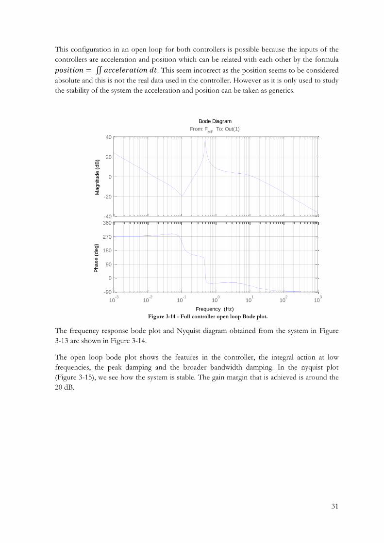
This configuration in an open loop for both controllers is possible because the inputs of the
controllers are acceleration and position which can be related with each other by the formula
∬ . This seem incorrect as the position seems to be considered
absolute and this is not the real data used in the controller. However as it is only used to study
the stability of the system the acceleration and position can be taken as generics.
The frequency response bode plot and Nyquist diagram obtained from the system in Figure
3-13 are shown in Figure 3-14.
The open loop bode plot shows the features in the controller, the integral action at low
frequencies, the peak damping and the broader bandwidth damping. In the nyquist plot
(Figure 3-15), we see how the system is stable. The gain margin that is achieved is around the
20 dB.
-40
-20
0
20
40
From: FMF
To: Out(1)
Magnitu
de (
dB
)
10-3
10-2
10-1
100
101
102
103
-90
0
90
180
270
360
Phase (
deg)
Bode Diagram
Frequency (Hz)
Figure 3-14 - Full controller open loop Bode plot.

32
-200
-150
-100
-50
0
50
From: Noise To: XMF
Magnitu
de (
dB
)
10-4
10-2
100
102
-90
0
90
180
270
Phase (
deg)
Bode Diagram
Frequency (Hz)
20
30
40
50
60
70
80
From: Noise To: FMF
Magnitu
de (
dB
)
10-4
10-2
100
102
0
90
180
270
Phase (
deg)
Bode Diagram
Frequency (Hz)
Figure 3-16 - Noise-Displacement frequency bode plots
3.2.4 Controller’s Results
Finally, the systems performance will be tested
to see how good it covers the design
specifications. In Figure 3-17 the closed loop
transmissibility and compliance plots (green)
are shown on top of the plants open loop plots
(blue) to show the improvements achieved.
The peak has been correctly damped and
shifted towards lower frequencies, in this case
to 0.2 Hz. The damping on higher frequencies
is an improvement in the isolation from
disturbances. The integral action from the
position controller can be seen in the
compliance as a decoupling from the Force
also at low frequencies starting at 0.01 Hz.
-20 -10 0 10 20 30 40 50 60-80
-60
-40
-20
0
20
40
60
80
0 dB
From: FMF
To: Out(1)
Nyquist Diagram
Real Axis
Imagin
ary
Axis
-5 -4 -3 -2 -1 0 1 2 3 4
-2
-1
0
1
2
30 dB
-10 dB
-6 dB
-4 dB
-2 dB
10 dB
6 dB
4 dB
2 dB
From: In(1) To: XMF
Nyquist Diagram
Real Axis
Imagin
ary
Axis
Figure 3-15 - Open Loop Nyquist plot.

33
Figure 3-16 shows the gain of the noise at different frequencies from the sensor to the
position of the metroframe. Logically the biggest gain in the noise will be around the
resonance where the controllers action is at its highest.
3.2.5 Conclusions
This method is highly intuitive and the relation between the results and the tuning process
itself is very strongly related. This gives a feel of control over the entire process. However,
reaching a balance on performance is not straightforward. In order to achieve the results just
described the number of iterations were very high, especially when the noise of the sensors
was added to the design because the number of variables to be taken into account were
doubled.
3.3 H-infinity Theory
The design process in the H-infinity methods is very different from the classical loopshaping
method seen previously. The way this method obtains its controllers and where the tuning
process lies will be shown in the following sections.
-250
-200
-150
-100
-50
0
50
From: XBF
To: X
MF
10-2
10-1
100
101
102
-180
-90
0
90
To: X
MF
From: FMF
10-2
10-1
100
101
102
Transmissibility and Compliance
Frequency (Hz)
Magnitu
de (
dB
) ; P
hase (
deg)
Figure 3-17 - Transmissibility and compliance of the classic loopshaping method controller

34
3.3.1 H-infinity norm
In the H-infinity method the controller is obtained through optimization algorithms. These
algorithms generate controllers that preserve internal stability while minimizing the H-infinity
norm of the system.
‖ ( )‖
( ( ))
The H-infinity norm seen above is the norm applied to a certain input output system, where
the norm is telling us the maximum gain of the frequency responses of the singular values of
the system i.e. the SISO interpretation of this norm is the maximum gain in the magnitude of
the frequency response of the system.
3.3.2 H-infinity design algorithms
The H-infinity algorithms make use of the following configuration of plant and controller
system shown in Figure 3-18, where the different signals
are:
w: Systems inputs
z: Systems outputs
u: Controllers output (actuators)
v: Controllers input (measurements)
The actual way that the H infinity controller design
algorithms generally work is the following. For the configuration of plant and controller
shown in Figure 3-18 an optimum achievable H-infinity value exists for the closed loop
transfers (w z). This value is unknown by the algorithm so it will try to approximate this
optimal value, thus not really obtaining an optimal controller but a good approximation. This
minimum H-infinity value obtained by the algorithm will be called gamma (γ). This gamma
will be obtained by iteratively giving a smaller value to gamma and studying the viability in
terms of stability and performance till a minimum is reached. Once the value is obtained the
algorithm will proceed to synthesize one of the infinite number of possible controllers for the
achieved gamma.
3.3.3 Augmented plant
As the controller is synthesized by the H-infinity algorithm the only way to add specifications
to that controller is by modifying the plant. This modification of the plant is done by adding
weighting functions to the inputs and outputs of the system as shown in Figure 3-19. The
blocks added (Ww and Wz) are matrices of filters for all inputs and outputs that give the
possibility to modify the closed loop transfer functions.
Figure 3-18 - H-infinity plant plus controller configuration
Augmented Plant
𝑧
Plant
Ww Wz 𝑤
𝑦 𝑢
Figure 3-19 - Augmented plant scheme
35
Adding gain to different frequencies in the weights will indicate that there has to be a tighter
control on those frequencies. It is equally important to specify frequencies where the
minimization is not necessary so to concentrate the control action on the bands of interest,
this is done by lower gains on the weights.
There will be a weighting function for each input to the plant, this is generally used to
characterize the inputs frequency response. Characterizing the inputs helps to optimize the
controller as there will be more control action at frequencies where the input has more gain.
The outputs from the plant and the frequencies at which they will have more or less gain are
given by the design requirements. For instance, if the acceleration of a system has to be
minimized at high frequencies the output z from the plant will be its acceleration and the
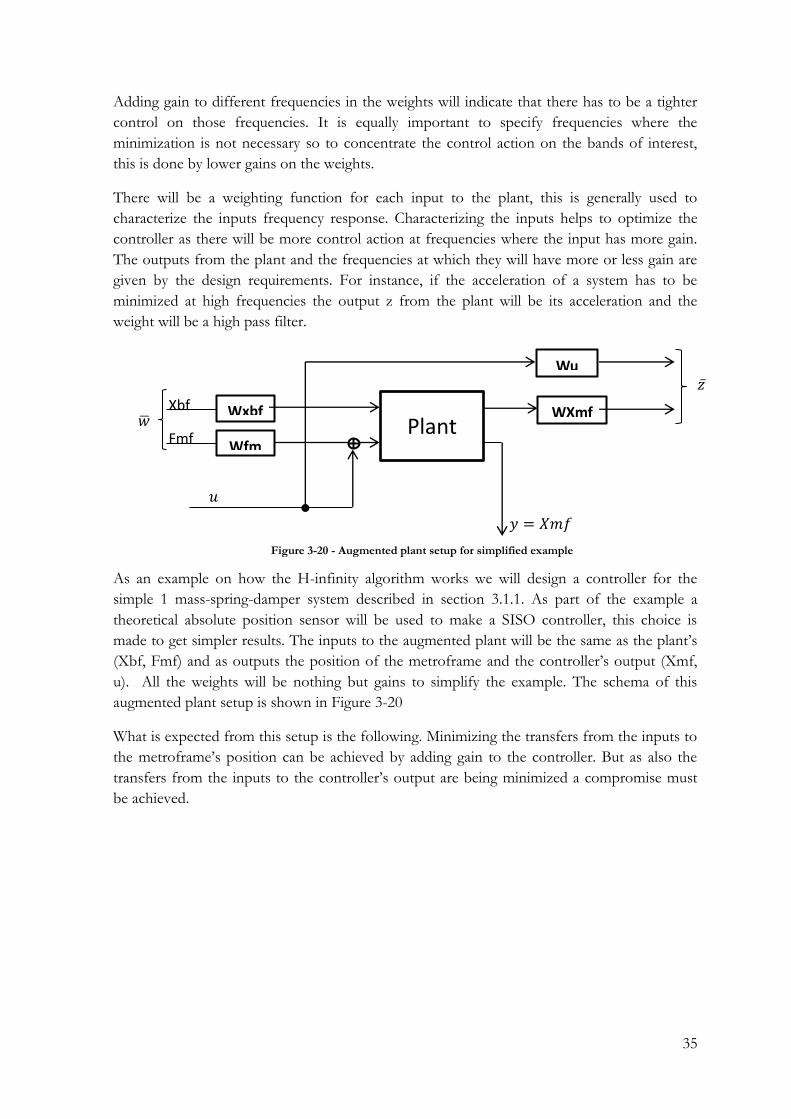
weight will be a high pass filter.
As an example on how the H-infinity algorithm works we will design a controller for the
simple 1 mass-spring-damper system described in section 3.1.1. As part of the example a
theoretical absolute position sensor will be used to make a SISO controller, this choice is
made to get simpler results. The inputs to the augmented plant will be the same as the plant‟s
(Xbf, Fmf) and as outputs the position of the metroframe and the controller‟s output (Xmf,
u). All the weights will be nothing but gains to simplify the example. The schema of this
augmented plant setup is shown in Figure 3-20
What is expected from this setup is the following. Minimizing the transfers from the inputs to
the metroframe‟s position can be achieved by adding gain to the controller. But as also the
transfers from the inputs to the controller‟s output are being minimized a compromise must
be achieved.
𝑢
Xbf
Fmf
Wxbf
WfmPlant
WXmf
Wu
Figure 3-20 - Augmented plant setup for simplified example
𝑤
𝑧
𝑦 𝑋𝑚𝑓

36
Figure 3-21 shows the loop without any controller (open loop) and on top the closed loop
with the H-infinity controller for every input to output of the augmented plant. This
comparison will let us see what the H-infinity algorithm tries to do with the transfer functions
of the augmented plant.
What happens is that the algorithm via means of the controller tries to minimize the transfer‟s
magnitude as much as possible. The stopping point is when adding more gain to the controller
will make the H-infinity norm increase its value instead of decreasing it. This is seen in our
example in the two left transfers, where adding gain would make the output to WU be bigger
in magnitude than the output to Wxmf.
On top of this minimization process which searches for the best performance the algorithm
will make sure that the system maintains its stability. A small detail to be noted, results for
vibration control would be excellent if the ideal absolute sensors as used for the example
existed.
3.3.4 Controllability and observability
Two properties that need to be fulfilled by the augmented plant in the design of a suitable H-
infinity controller are controllability and observability (Skogestad & Postelwaith). These
properties are defined as follows
Controllability – A system is considered controllable if and only if the system states can be varied by
changing the systems input.
-200
-150
-100
-50
0
50
From: XBF
To: W
XM
F
100
102
-120
-100
-80
-60
-40
To: W
U
From: FMF
100
102
Augmented Plant closed loops
Frequency (Hz)
Magnitu
de (
dB
)
No controller
H-inf Controller
Figure 3-21 - Augmented plat’s open Loop and H-infinity controller’s closed loop comparison.
-40 dB
-40 dB

37
Observability – A system is considered observable if and only if the initial state can be determined
from the observed system’s output through an interval of time for all the internal states.
Both these conditions have to be met by the augmented plant from the controller‟s point of
view, in order to be able to generate a stabilizing controller. The following analytical
procedures can be used.
For both the controllability and observability the matrices from the state space representation
will be used. Formerly {
where:
x is the state vector
y is the output vector
A is the states matrix
B is the input matrix
C is the output matrix
D is the feedforward matrix.
The A, B, C, D matrices enable us to easily characterize any model with two equations
independently from the amount of partial differential equations it may be composed of.
To determine controllability we will need to obtain the controllability matrix. And the system will be considered controllable when the controllability matrix is full rank. The controllability matrix is defined as follows, where A and B are the A,B matrices of the state-space description, p is the number of inputs and q the number of states.
Observability has an analog analysis to controllability. In this case the observability matrix will
be created. The system will be considered observable if the matrix is full rank. C and A are the
C, A matrices of the state space description and p is the number of inputs.
Observability and controllability are achieved for all augmented plants designed in the
following sections.
3.3.5 Robust stability analysis.
Once a controller has been designed it is necessary to check for robust stability. The small gain
theorem provides tools to do so, stated as following:

38
Let W1, W2 ϵ RH∞, PΔ=P0 + Δ for Δ ϵ RH∞ and K be a stabilizing controller
for P0. Then K is robustly stabilizing for all Δ ϵ 1/γ∙βRH∞
If and only if ||W2KSOW1||∞< γ
Where γ is the H-infinity value from 3.3.2 and RH∞ is the H infinity space which consists of all
proper and real rational stable transfer matrices.
What this property says is that for additive uncertainties a system that is nominally stable with
a certain maximum gain (γ) will also be robustly stable if the maximum gain of the disturbed
plant falls beneath 1. This theorem allows guaranteeing robust stability for unstructured
uncertainties. The problem with this kind of statement is that because of the unstructured
nature of the uncertainty the margin given to provide the robustness can be too conservative.
Because we know that the gamma value is the maximum gain of the system at just one
frequency we can make this statement more precise by extending it to more frequencies. In a
SISO system this can be seen as shown in the following example.
The zone marked in green would be were the uncertainity
of this random transfer function would be allowed to be
to keep robust stability in the system.
In the case of MIMO systems the visualization is not
possible as the maximum gain of the full system doesn‟t
Figure 3-22 - Example of allowable uncertainty in a SISO system
Figure 3-23 - Uncertainties in the LFT configuration.

39
have a graphical visualization. However in the disposition of Figure 3-23 (where M is the
closed loop of plant and controller) if the uncertainty has a structured nature it can be “pulled
out” of the system and visualized in the same fashion as the SISO systems.
3.4 Method 2: Minimization of metroframe’s movement design
To use the metroframe‟s absolute position to be minimized by the controller as seen in Figure
2-1. This approach has been used in (Wal & Heertjes) as base controller design method to
elaborate its study. In (Nakashima, Tsujino, & Fuji, 1996), (Pantazi, Sebastian, Pozidis, &
Eleftheriou, 2005)and (Watanabe & al., 1996) similar approaches are used, the idea is making
use of the optimal capabilities of the H-infinity method to minimize one of the variables in the
system. This seems like the obvious approach to H-infinity and that is why it has been
extensively used in applications in search of alternative methods of control.
The effect of changing the different weightings is the following
WXmf: Filters the frequency response of the position of the metroframe. Adding gain
to this weight will increase the control action at the selected frequencies. This weight is
the base for adding design requisites to the system in this configuration.
Wu: Affects the magnitude of the controllers. Adding gain to this weight reduces the
control action. Helps to set boundaries in frequency to limit the action of the
controllers in regions of less interest.
WXbf and WFmf: Related directly to the transmissibility and compliance. These
weights will be shaped to represent the actual behaviour of the inputs baseframe
movement and force to the metroframe.
WposN and WaccN: They will describe the real behaviour of the noises of the
sensors and reduce the controllers output where the noise is bigger in magnitude.
Figure 3-24 - Augmented plant for minimization of the metroframe
Xbf
Fmf
u
WXbf
WFmf Plant
y
WaccN Accnoise
Posnoise
WXmf
Wu
WposN

40
3.4.1 Weights used
The following weights have been applied.
Output weights:
Wxmf::{
( )
( )
( )
Our interest is centred from the
resonance frequency until around 100 Hz.
The passive response of the plant
decreases with a -2 slope from its
resonance frequency at 0.5 Hz. This
means that in the closed loop this slope is
also present reducing the importance for
the H-infinity algorithm of higher
frequencies at a rate of -40 dB per decade.
To even out the weight for all the band of
interest a +2 slope will be added from 0.5
Hz to a 100 Hz evening out the frequency
response for our region of interest, the result can be seen in Figure 3-25. On top of
this a high pass filter will be added. This filter will be used to emphasize the region of
interest building a difference in gain between low frequencies (less interesting) and
high frequencies (more interesting).
Wu: {
( )
( )
( )
This weight will be a first order high pass filter that will deal with unwanted control
action at high frequencies. The cut off frequency will be at 250 Hz. The gain of this
weight has been chosen through trial and error to obtain the desired results.
The input weights:
WXbf and WFmf: * ( )
Both these weights are just gains that relate to the inputs magnitudes 10 micrometers
for the baseframe‟s position movement and 10 Newton for the Force to the
metroframe.
WPosNoise: * ( )
Just a gain in order to replicate white noise.
100
102
-200
-150
-100
-50
From: FMF
To: XMF
Magnitu
de (
dB
)
Bode Diagram
Frequency (Hz)
Without w eight
With w eight
Figure 3-25 - Effect of evening out compliance´s -2 slope

41
WAccNoise: {
( )
( )
( )
The noise of the accelerometer is a √ ramp that decreases until 5Hz.
3.4.2 Results
In Figure 3-26 you can see the obtained transmissibility and compliance.
The transmissibility is worse in the closed loop than what the passive system offers and the
compliance doesn‟t show a big improvement. The result for transmissibility is obtained
because the algorithm decides that adding gain to the position loop - even though
transmissibility is worsened - is worth to reduce the H-infinity norm of the system.
The next figure (Figure 3-27) shows the open loop of the final implementation of controller
and plant. What is worth noticing here is the bandwidth of the system, this is determined by
10-1
100
101
102
103
-200
-150
-100
-50
0
From: XBF
To: X
MF
10-1
100
101
102
103
From: FMF
LMI - Transmissibility and Compliance - Gamma=0.56014
Frequency (Hz)
Magnitu
de (
dB
)
Open Loop passive
Closed Loop active
Figure 3-26 - Obtained transmissibility and compliance for the minimization of position approach
10-1
100
101
102
103
-120
-100
-80
-60
-40
-20
0
20
40
60
From: FMF
To: Out(1)
Magnitu
de (
dB
)
Open Loop
Frequency (Hz)
Position Loop
Acceleration Loop
Total
Figure 3-27 - Open loop for the minimization of position approach

42
the last frequency where the open loop falls below the 0dB, in the shown figure this happens
at 200Hz. This bandwidth is result of the weight on the controller output (Wu), without this
weight the bandwidth goes up to 10kHz.
Robust stability analysis
The controlled system with the controller obtained by this method is robustly stable if the
uncertainties obey the following rules.
The maximum allowable uncertainty gain for structured uncertainties for each input and
output is shown in Figure 3-28
The minimum gain for any input to output response at each frequency is the limit of the
maximum allowable unstructured uncertainty. This is shown in Figure 3-29. The maximum H-
infinity norm for the uncertainty must be lower than 1/gamma < 1.7852
0
20
40
60
80
100
120
140
From: XBF
To:
X MF
100
0
50
100
150
200
To:
Actu
ato
r F
orc
e
From: FMF
100
From: PosNoise
100
From: AccNoise
100
Allowable uncertainty
Frequency (rad/sec)
Mag
nitud
e (
dB
)
Figure 3-28 – Structured uncertainty limit for each input and output of the system.

43
3.4.3 Conclusions
The results on transmissibility and compliance are worse with this method compared to the
classic loopshaping method. Even the passive system delivers better results for transmissibility
than this controller. However, the tuning process was not so exhaustive, mainly because of the
lack of information on the frequency responses of the inputs. Having this information would
help to optimize the output. The exact reason is that without more precise information the
disturbances are assumed to be very broadband and therefore ask for control power at high
frequencies affecting therefore the output in the band of interest.
3.5 Method 3: Shaping with desired compliance and transmissibility design
10-1
100
101
102
103
0
5
10
15
20
25
30
35
40
45From: Actuator Force To: Out(1)
Mag
nitud
e (
dB
)
Maximum unstructured uncertainty
Frequency (rad/sec)
Figure 3-29 - Unstructured uncertainty limit of the system
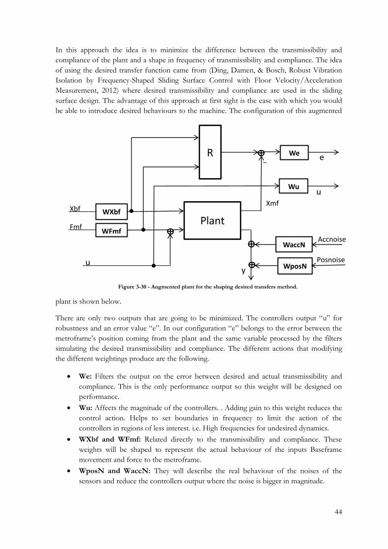
44
In this approach the idea is to minimize the difference between the transmissibility and
compliance of the plant and a shape in frequency of transmissibility and compliance. The idea
of using the desired transfer function came from (Ding, Damen, & Bosch, Robust Vibration
Isolation by Frequency-Shaped Sliding Surface Control with Floor Velocity/Acceleration
Measurement, 2012) where desired transmissibility and compliance are used in the sliding
surface design. The advantage of this approach at first sight is the ease with which you would
be able to introduce desired behaviours to the machine. The configuration of this augmented
plant is shown below.
There are only two outputs that are going to be minimized. The controllers output “u” for
robustness and an error value “e”. In our configuration “e” belongs to the error between the
metroframe‟s position coming from the plant and the same variable processed by the filters
simulating the desired transmissibility and compliance. The different actions that modifying
the different weightings produce are the following.
We: Filters the output on the error between desired and actual transmissibility and
compliance. This is the only performance output so this weight will be designed on
performance.
Wu: Affects the magnitude of the controllers. . Adding gain to this weight reduces the
control action. Helps to set boundaries in frequency to limit the action of the
controllers in regions of less interest. i.e. High frequencies for undesired dynamics.
WXbf and WFmf: Related directly to the transmissibility and compliance. These
weights will be shaped to represent the actual behaviour of the inputs Baseframe
movement and force to the metroframe.
WposN and WaccN: They will describe the real behaviour of the noises of the
sensors and reduce the controllers output where the noise is bigger in magnitude.
We
Plant
R
Xbf
Fmf
u y
Xmf WXbf
WFmf
e
Wu u
Figure 3-30 - Augmented plant for the shaping desired transfers method.
WaccN Accnoise
Posnoise WposN

45
3.5.1 Desired transmissibility and compliance
The desired transmissibility and compliance can be seen in Figure 3-31.
For both transmissibility and compliance the resonant peak is shifted from 0.5Hz to 0.3Hz.
For transmissibility the desired plant differs from the passive system till infinite high
frequencies, this would mean to have a controller that has loop gain until infinitely high
frequencies. This is not a reasonable assumption as the control for high frequencies has to be
avoided. However, it is important to realize that these desired transmissibilities and
compliances are just demands for the controller and that they will be approximated by the
controller‟s action within its limits and not necessarily followed precisely.
The demands for compliance are: preserved stiffness represented by the horizontal line at low
frequencies and reduced effect of the force for the frequencies above the resonance peak.
3.5.2 Weights used
Output weights:
10-2
100
102
-200
-150
-100
-50
0
From: XBF
To: X
MF
10-2
100
102
From: FMF
Transmissibility and compliance in R and plant
Frequency (Hz)
Magnitu
de (
dB
)
Passive system
Desired Transfers
Figure 3-31 - Desired transmissibility and compliance

46
We: {
( )
( )
( )
The reason for adding this growing slope for the output error is represented in Figure
3-32. The difference between the desired transmissibility and compliance may seem
equal in decibels, but is not in the absolute scale. The H-infinity norm is calculated for
the absolute values. Therefore this weight is added to compensate for the natural
decreasing slope of the system and so evening the difference from 0.5Hz up to 100Hz
that is where our region of interest lies.
Wu:{
( )
( )
( )
This weight will be a second order high pass filter that will deal with unwanted control
action at high frequencies. The cut off frequency will be at 250 Hz. The gain is chosen
by tuning.
The input weights:
WXbf and WFmf: * ( )
Both these weights are just gains that relate to the inputs magnitudes 10 micrometers
for the baseframes position and 10 Newton for the Force to the metroframe.
WposN:* ( )
Just a gain with the idea to replicate white noise.
10-2
10-1
100
101
102
103
-120
-100
-80
-60
-40
-20
0
20
40
From: XBF
To: XMF
Magnitu
de (
dB
)
Bode Diagram
Frequency (Hz)Figure 3-32 - Absolute difference versus logarithmic difference in bode plot.
10db(diff) = 0.1 absolute diff aprox.
10db(diff) = 0.001 absolute diff
aprox.

47
WaccN:{
( )
( )
( )
The noise of the accelerometer is a √ ramp that starts at 5Hz.
3.5.3 Results
The following figures show the results obtained with this method. Figure 3-33 shows the
obtained transmissibility and compliance in comparison with the passive and the desired plots.
The controlled response shows a good approximation to the desired transfers. For compliance
the obtained result almost mimics the desired plant‟s behaviour. For transmissibility the
response is not exactly the same as the desired response but it is still a big improvement. The
resonant peak has been shifted and damped correctly while there is still a reduction in the
magnitude for frequencies up to 100Hz.
10-1
100
101
102
103
-140
-120
-100
-80
-60
-40
-20
0
20
40
From: FMF
To: Out(1)
Magnitu
de (
dB
)
Open Loop
Frequency (Hz)
Position Loop
Acceleration Loop
Complete Loop
Figure 3-34 - Open loop for the desired transfers approach.
10-1
100
101
102
103
-200
-150
-100
-50
0
From: XBF
To: X
MF
10-1
100
101
102
103
From: FMF
LMI - Transmissibility and Compliance - Gamma=0.80009
Frequency (Hz)
Magnitude (
dB
)
Open Loop passive
Wanted
Closed Loop active
Figure 3-33 - Transmissibility and Compliance from the desired plant approach
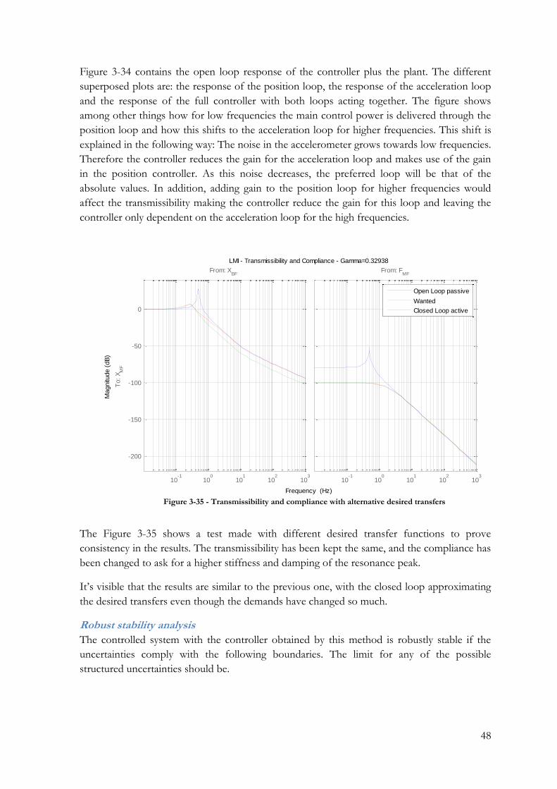
48
Figure 3-34 contains the open loop response of the controller plus the plant. The different
superposed plots are: the response of the position loop, the response of the acceleration loop
and the response of the full controller with both loops acting together. The figure shows
among other things how for low frequencies the main control power is delivered through the
position loop and how this shifts to the acceleration loop for higher frequencies. This shift is
explained in the following way: The noise in the accelerometer grows towards low frequencies.
Therefore the controller reduces the gain for the acceleration loop and makes use of the gain
in the position controller. As this noise decreases, the preferred loop will be that of the
absolute values. In addition, adding gain to the position loop for higher frequencies would
affect the transmissibility making the controller reduce the gain for this loop and leaving the
controller only dependent on the acceleration loop for the high frequencies.
The Figure 3-35 shows a test made with different desired transfer functions to prove
consistency in the results. The transmissibility has been kept the same, and the compliance has
been changed to ask for a higher stiffness and damping of the resonance peak.
It‟s visible that the results are similar to the previous one, with the closed loop approximating
the desired transfers even though the demands have changed so much.
Robust stability analysis
The controlled system with the controller obtained by this method is robustly stable if the
uncertainties comply with the following boundaries. The limit for any of the possible
structured uncertainties should be.
10-1
100
101
102
103
-200
-150
-100
-50
0
From: XBF
To: X
MF
10-1
100
101
102
103
From: FMF
LMI - Transmissibility and Compliance - Gamma=0.32938
Frequency (Hz)
Magnitu
de (
dB
)
Open Loop passive
Wanted
Closed Loop active
Figure 3-35 - Transmissibility and compliance with alternative desired transfers
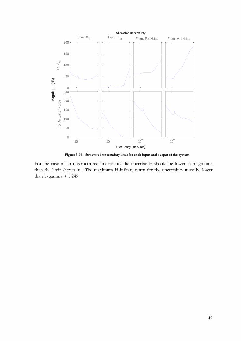
49
For the case of an unstructrured uncertainty the uncertainty should be lower in magnitude
than the limit shown in . The maximum H-infinity norm for the uncertainty must be lower
than 1/gamma < 1.249
0
50
100
150
200
From: XBF
To:
X MF
100
0
50
100
150
200
250
To:
Actu
ato
r F
orc
e
From: FMF
100
From: PosNoise
100
From: AccNoise
100
Allowable uncertainty
Frequency (rad/sec)
Mag
nitud
e (
dB
)
Figure 3-36 - Structured uncertainty limit for each input and output of the system.

50
3.5.4 Conclusions
This method allows us to easily shape the transmissibility and compliance of our system. The
results are comparable to the classical loopshaping method. And the tuning process is very
easy compared to the previous h-infinity method. The need of previous information on the
plants behaviour is not so high and this affects the tuning process making it far more
manageable.
One drawback on this method is that the optimality advantages of H-infinity are lost. The fact
of predesigning the transfer functions creates pre-established limitations to the isolation
capabilities of the system, more or less in the same fashion as with the classical methods.
3.6 Conclusions The new method created for controller design has showed us that it is possible to adapt the
optimal H-infinity method to become easier to tune without any loss in performance in
comparison to the classical loopshaping method. This method also gives the great advantage
of being scalable to MIMO while the classical method isn‟t.
Compared to the straightforward approach of the H-infinity method the new method needs a
lot less previous information on the behaviour of the plant leaving it more flexible to adapt to
unknown environments. But in both cases the results could improve a lot if more information
was provided, information on the frequency spectrums of the inputs or on known
uncertainties.
10-1
100
101
102
103
0
2
4
6
8
10
12
14
16From: Actuator Force To: Out(1)
Mag
nitud
e (
dB
)
Maximum unstructured uncertainty
Frequency (rad/sec)
Figure 3-37 - Unstructure uncertainty limit for the controlled system.
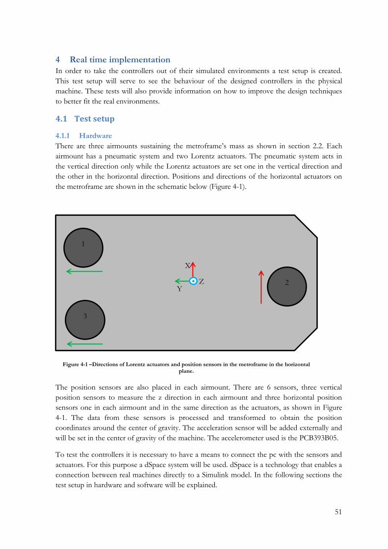
51
4 Real time implementation
In order to take the controllers out of their simulated environments a test setup is created.
This test setup will serve to see the behaviour of the designed controllers in the physical
machine. These tests will also provide information on how to improve the design techniques
to better fit the real environments.
4.1 Test setup
4.1.1 Hardware
There are three airmounts sustaining the metroframe‟s mass as shown in section 2.2. Each
airmount has a pneumatic system and two Lorentz actuators. The pneumatic system acts in
the vertical direction only while the Lorentz actuators are set one in the vertical direction and
the other in the horizontal direction. Positions and directions of the horizontal actuators on
the metroframe are shown in the schematic below (Figure 4-1).
The position sensors are also placed in each airmount. There are 6 sensors, three vertical
position sensors to measure the z direction in each airmount and three horizontal position
sensors one in each airmount and in the same direction as the actuators, as shown in Figure
4-1. The data from these sensors is processed and transformed to obtain the position
coordinates around the center of gravity. The acceleration sensor will be added externally and
will be set in the center of gravity of the machine. The accelerometer used is the PCB393B05.
To test the controllers it is necessary to have a means to connect the pc with the sensors and
actuators. For this purpose a dSpace system will be used. dSpace is a technology that enables a
connection between real machines directly to a Simulink model. In the following sections the
test setup in hardware and software will be explained.
1
3
2
Figure 4-1 –Directions of Lorentz actuators and position sensors in the metroframe in the horizontal plane.
Y
X
Z
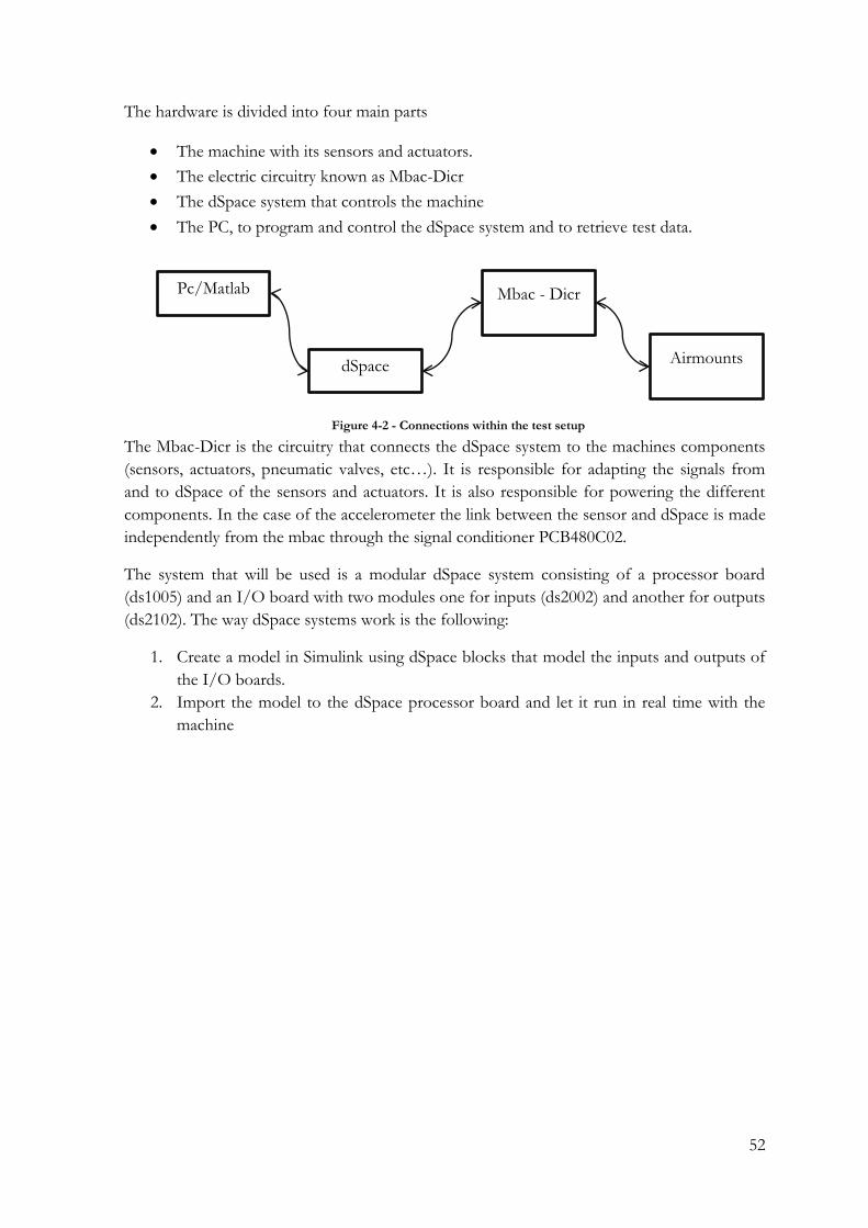
52
The hardware is divided into four main parts
The machine with its sensors and actuators.
The electric circuitry known as Mbac-Dicr
The dSpace system that controls the machine
The PC, to program and control the dSpace system and to retrieve test data.
The Mbac-Dicr is the circuitry that connects the dSpace system to the machines components
(sensors, actuators, pneumatic valves, etc…). It is responsible for adapting the signals from
and to dSpace of the sensors and actuators. It is also responsible for powering the different
components. In the case of the accelerometer the link between the sensor and dSpace is made
independently from the mbac through the signal conditioner PCB480C02.
The system that will be used is a modular dSpace system consisting of a processor board
(ds1005) and an I/O board with two modules one for inputs (ds2002) and another for outputs
(ds2102). The way dSpace systems work is the following:
1. Create a model in Simulink using dSpace blocks that model the inputs and outputs of
the I/O boards.
2. Import the model to the dSpace processor board and let it run in real time with the
machine
Airmounts
Mbac - Dicr
dSpace
Pc/Matlab
Figure 4-2 - Connections within the test setup

53
The dSpace system is the link between the hardware and the software so from the point the
signals reach the dSpace system it all runs in software.
Figure 4-3 - Accelerometer and signal conditioner
Figure 4-4 - Input and output board of the dSpace system

54
4.1.2 Software
In order to test the designed controllers a simulink model is created to close the loop between
the sensors and the machine. The model consists of the following parts.
Controller module
Pneumatic controllers
Lorentz controllers
Controller module
The controller module initializes the system. This means lifting the mass from the ground and
enabling the control loops. The order is the following:
1. Inflate the airmounts by opening the valves until the mass is no longer touching the
ground.
2. Enable the pneumatic controller to maintain the mass floating between the two
endpoints of the airmounts
3. Once the mass is stable enough enable the Lorentz controller.
This routine accelerates the initialization of the system and also prevents the Lorentz
controllers from using unnecessary force and possibly overheating i.e. when the machine is
not yet suspended the Lorentz motors would try to lift the 2 ton mass.
The control module is made with stateflow, it creates a finite state machine within the
simulink model. In this case the module receives information on the position of the machine
and reacts by setting offset values on the valves of the pneumatic system and enabling
systematically the controlled loops.
Pneumatic and Lorentz controllers
The pneumatic and Lorentz controllers are made out of 9 independent controllers for each
coordinate they control. Three controllers for the pneumatic control system and six for the
Lorentz control system.
setpoint physical _2_logical
OT_MS_6x6_IN 1
OT_MS_6x6_IN 2
OT_MS_6x6_IN 3
OT_MS_6x6_IN 4
OT_MS_6x6_IN 5
OT_MS_6x6_IN 6
OT_MS_6x6_OUT 1
OT_MS_6x6_OUT 2
OT_MS_6x6_OUT 3
OT_MS_6x6_OUT 4
OT_MS_6x6_OUT 5
OT_MS_6x6_OUT 6
sensor_interface
H1
V1
H2
V2
H3
V3
Out 1
Out 2
Out 3
Out 4
Out 5
Out 6
pneumatic actuator
interface
In 2
In 4
In 6
v 1
v 2
v 3
measurement system position
OT_MS_6x6_IN 1
OT_MS_6x6_IN 2
OT_MS_6x6_IN 3
OT_MS_6x6_IN 4
OT_MS_6x6_IN 5
OT_MS_6x6_IN 6
OT_MS_6x6_OUT 1
OT_MS_6x6_OUT 2
OT_MS_6x6_OUT 3
OT_MS_6x6_OUT 4
OT_MS_6x6_OUT 5
OT_MS_6x6_OUT 6
lorentz actuator system
OT_AS_6x6_IN 1
OT_AS_6x6_IN 2
OT_AS_6x6_IN 3
OT_AS_6x6_IN 4
OT_AS_6x6_IN 5
OT_AS_6x6_IN 6
OT_AS_6x6_OUT 1
OT_AS_6x6_OUT 2
OT_AS_6x6_OUT 3
OT_AS_6x6_OUT 4
OT_AS_6x6_OUT 5
OT_AS_6x6_OUT 6
lorentz actuator interface
In 1
In 2
In 3
In 4
In 5
In 6
h1
v 1
h2
v 2
h3
v 3
error measure pneumatic
Setpoint _V1Measured _V1Setpoint _V2
Measured _V2Setpoint _V3Measured _V3
error_V1
error_V2
error_V3
error measure logical
Setpoint _x
Measured _x
Setpoint _y
Measured _y
Setpoint _rz
Measured _rz
Setpoint _z
Measured _z
Setpoint _rx
Measured _rx
Setpoint _ry
Measured _ry
error_x
error_y
error_rz
error_z
error_rx
error_ry
dspace_in
-K-
Switch
Stateflow _control
position _sensor _v 1
position _sensor _v 2
position _sensor _v 3
EndSwitch
pneumatic _stable
Lorentz _enable
valve _offset _1
valve _offset _2
valve _offset _3
EnableLorentzControler
EnablePneumaticControler
Setpoints
[H1 V1 H2 V2 H3 V3]
-C-
RTI Data
Pre_ControllerPost_Noise
Post_Controller
Pneumatic controller
pneu _v 1_error
pneu _v 2_error
pneu _v 3_error
pneu_v 1_out
pneu_v 2_out
pneu_v 3_out
PneumStable
1
Lorentz _enable
0
Lorentz position controller
ctrl _in_x
ctrl _in_y
ctrl _in_rz
ctrl _in_z
ctrl _in_rx
ctrl _in_ry
ctrl _out _x
ctrl _out _y
ctrl _out _rz
ctrl _out _z
ctrl _out _rx
ctrl _out _ry
LTI System
Noise_filter
Inflate /Deflate
1
Ground 2
Ground 1
Ground
DS2102 _B2
Bad Link
DS2102 _B1
Bad Link
DS2002 _B1
Bad Link
Control _Out _Enable
1Constant
0
Band -Limited
White Noise
Acceleration offset
-C-
Accelero Data
Figure 4-5 - Stateflow chart for the initialization of the system

55
The three controllers working for the pneumatic system work in parallel. One controller for
each airmount „s vertical direction. These controllers are in charge of positioning the mass at
the correct height. They operate at very low frequencies leaving the active isolation to the
Lorentz actuators. The information they receive is directly the position coming from the
sensors in each airmount.
From the six controllers for the Lorentz actuators each controller operates on one of the
coordinates that the machine can move on, these are the three displacement coordinates
(x,y,z) and the three rotational coordinates (χ, ψ, φ). In order to use information of the
position of the metroframe in its center of gravity a transformation matrix needs to be used to
translate the information coming from the position sensors at each airmount to the desired
position.
pneu _v3_out
3
pneu _v2_out
2
pneu _v1_out
1
pneumatic _controller _v3
OT_CO_CTL _IN
OT_CO _CTL_OUT
P_out
I_out
pneumatic _controller _v2
OT_CO_CTL _IN
OT_CO _CTL_OUT
P_out
I_out
pneumatic _controller _v1
OT_CO_CTL _IN
OT_CO _CTL_OUT
P_out
I_out
Terminator 5
Terminator 4
Terminator 3
Terminator 2
Terminator 1
Terminator
Enable
pneu _v3_error
3
pneu _v2_error
2
pneu _v1_error
1
Figure 4-6 - Pneumatic controllers on the Simulink model
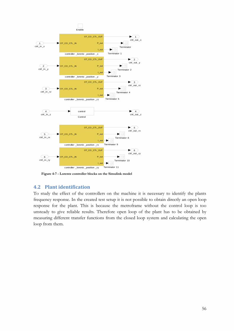
56
4.2 Plant identification To study the effect of the controllers on the machine it is necessary to identify the plants
frequency response. In the created test setup it is not possible to obtain directly an open loop
response for the plant. This is because the metroframe without the control loop is too
unsteady to give reliable results. Therefore open loop of the plant has to be obtained by
measuring different transfer functions from the closed loop system and calculating the open
loop from them.
ctrl_out _ry
6
ctrl_out _rx
5
ctrl_out _z
4
ctrl_out _rz
3
ctrl_out _y
2
ctrl_out _x
1
controller _lorentz _position _y
OT_CO_CTL _IN
OT_CO _CTL_OUT
P_out
I_out
controller _lorentz _position _x
OT_CO_CTL _IN
OT_CO _CTL_OUT
P_out
I_out
controller _lorentz _position _rz
OT_CO_CTL _IN
OT_CO _CTL_OUT
P_out
I_out
controller _lorentz _position _ry
OT_CO_CTL _IN
OT_CO _CTL_OUT
P_out
I_out
controller _lorentz _position _rx
OT_CO_CTL _IN
OT_CO _CTL_OUT
P_out
I_out
Terminator 9
Terminator 8
Terminator 5
Terminator 4
Terminator 3
Terminator 2
Terminator 11
Terminator 10
Terminator 1
Terminator
Control
control
Enable
ctrl_in_ry
6
ctrl_in_rx
5
ctrl_in_z
4
ctrl_in_rz
3
ctrl_in_y
2
ctrl_in_x
1
Figure 4-7 - Lorentz controller blocks on the Simulink model

57
To obtain these closed loop transfer functions, white Gaussian noise will be added to the
loop as shown in the schematic in Figure 4-8. The transfer functions that can be obtained are
the frequency responses from the input (wgn) to the three outputs shown in the schematic
(a,b,c). The transfer functions obtained are the following:
−
( )
b
−
( )
*P = plants transfer function; C = controller transfer function; n = noise input.
To obtain P the following can be done
−
−
The obtained transfer function for the plant is the response from the force of the actuators to
the position of the metroframe. This is the compliance of the plant. The transmissibility
cannot be obtained because it is not possible to add noise to the floor vibrations.
In the case of the frequency response from the force to the acceleration of the metroframe it
is possible to directly read the information from the accelerometer in an open loop. This is
because the metroframe is already controlled by the position control loop and the
accelerometer is set independent from the loop.
To obtain the plants frequency response a measurement of 15 minutes has been made with a
white Gaussian noise of 5N amplitude in the Lorentz actuator.
Controller Plant
Figure 4-8 – Gaussian noise added to the closed loop within the dspace environment
-
WGN
dSpace environment
a
b c

58
The process shown in Figure 4-9 has been used to obtain the frequency response. The
measured signal is divided into pieces, in this case in 15 parts of 60 seconds each. Each signal
is filtered and then its Fourier transform is calculated. Finally the frequency responses of each
piece are merged together. The result is a frequency response where the external noises are
reduced. This process is used to calculate all the frequency responses needed to calculate the
plant (a,b,c and n) as shown before.
4.2.1 Non-linearity’s and limitations in the setup
In the real setup there are some nonliearity‟s that were not present in the simulation
environment and may affect the output of the plant‟s identification. These non-linearity‟s are
saturation levels of the actuators, maximum metroframe displacements, sensor errors and
sampling rates.
Actuator saturation levels
The saturation levels of the actuators limit the maximum amount of newton of force the
actuators can generate. These saturation levels are not only limited by the capacity of the
actuators but its limit is set even lower by the software. This is done to avoid excessive force
output that could overheat the Lorentz actuators. The saturation levels are set to be ±10N for
the vertical actuators of each airmount.
In the simulated environment there was no limitation on the amount of force the controllers
could ask the actuators to apply. Thus this will bring problems when applying the created
controllers to the real time environment.
0 100 200 300 400 500 600 700 800 900-4
-2
0
2
4x 10
-4
900s
0 1 2 3 4 5 6
x 104
-2
0
2x 10
-4
60s
…
0 1 2 3 4 5 6
x 104
-2
0
2
4x 10
-4
60s
1.
15.
Hanning Filter
+ Fourier
transform
Mean
Figure 4-9 - Process used to obtain cleaner frequency responses from measured data
Hanning Filter
+ Fourier transfor

59
Metroframe’s end stops
The metroframe has limited movement in all directions. The maximum displacement is
around ±2cm around the centre for the vertical direction. This limits the amount of input
noise that is used for the identification.
In the simulations the displacement was around the micrometers so this limitation should not
affect the controlled system.
Sensor errors
The accelerometer sensor used has an unexpected offset. This offset does not affect the
identification. However, this offset although small affects the controllers behaviour. The
effects on the output of the controllers from this offset have been tested in the simulated
environment. The offset is seen by the controllers as a great acceleration at the start producing
a peak as an initial response. After this the ouput is steady and the offset is no longer a
problem.
There are two possible solutions for this problem. One would be to connect the controllers to
the sensors without closing the loop until the controllers output is stabilized. And the other
would be to calculate the offset and manually eliminate it from the accelerometer‟s signal by
substraction. Because the offset is steady in between measurements the latter solution has
been used.
Sampling rates
In the design controllers have been assumed to be in continuous time. In the real time
implementation because there is a need to digitalize the information sampling rates exist.
These sampling rates limit the maximum frequencies at which the controllers can operate.
The sampling rate of the machine is 1250 Hz. This frequency lies higher than the bandwidth
of interest of our design. However, in the case of the H-infinity methods the controllers have
poles and zeros lying beyond this frequency. These high frequency poles and zeros generate
unexistent peaks in the frequency responses.
In order to prevent strange behaviours coming from the undersampling of the high
frequencies in the machine when run through the controllers, the poles from the controllers
with frequencies higher than 100Hz have been eliminated. The results of this reduction are
shown in Figure 4-10.

60
This reduction brings no changes to the magnitude or the phase of the frequency response for
frequencies lower than 100 Hz.
4.2.2 Identification results
The magnitude, phase and coherence of the frequency responses are shown in Figure 4-11
and Figure 4-12.
The obtained frequency responses of the plant of the real time machine are shown in. The
responses are linear for the frequencies between the 0.1 Hz and 10 Hz. Above and below
these frequencies the coherence is reduced for the following reasons.
For the low frequencies this comes from the size of the samples used to obtain the
frequency response. The bigger the data string of the sample the better resolution at
lower frequencies you can get. The limit is set by 1/(data length) in this case 1/45 =
0.0222 Hz
For the higher frequencies this is due to mechanics that produce nonlinear behaviours.
In the case of the acceleration, the increasing magnitude at low frequencies comes
from the noise from the accelerometer.
Figure 4-10 - Results from high frequency pole elimination in H-infinity controllers
-200
-150
-100
-50
0
50
100
System: controlzpk
I/O: In(1) to Out(1)
Frequency (Hz): 20.5
Magnitude (dB): 53.4
From: In(1)
To: O
ut(
1)
10-2
100
102
104
-360
-270
-180
-90
0
90
180
270
360
450
To: O
ut(
1)
From: In(2)
10-2
100
102
104
Bode Diagram
Frequency (Hz)
Magnitu
de (
dB
) ; P
hase (
deg)

61
10-2
10-1
100
101
102
103
-300
-200
-100
0M
agnitude [
dB
]
Force to Position frequency response
10-2
10-1
100
101
102
103
-200
0
200
Phase [
deg]
10-2
10-1
100
101
102
103
0
0.5
1
Cohere
nce [
-]
Freq [Hz]
Figure 4-11 - Measured plant frequency response from Force to Position
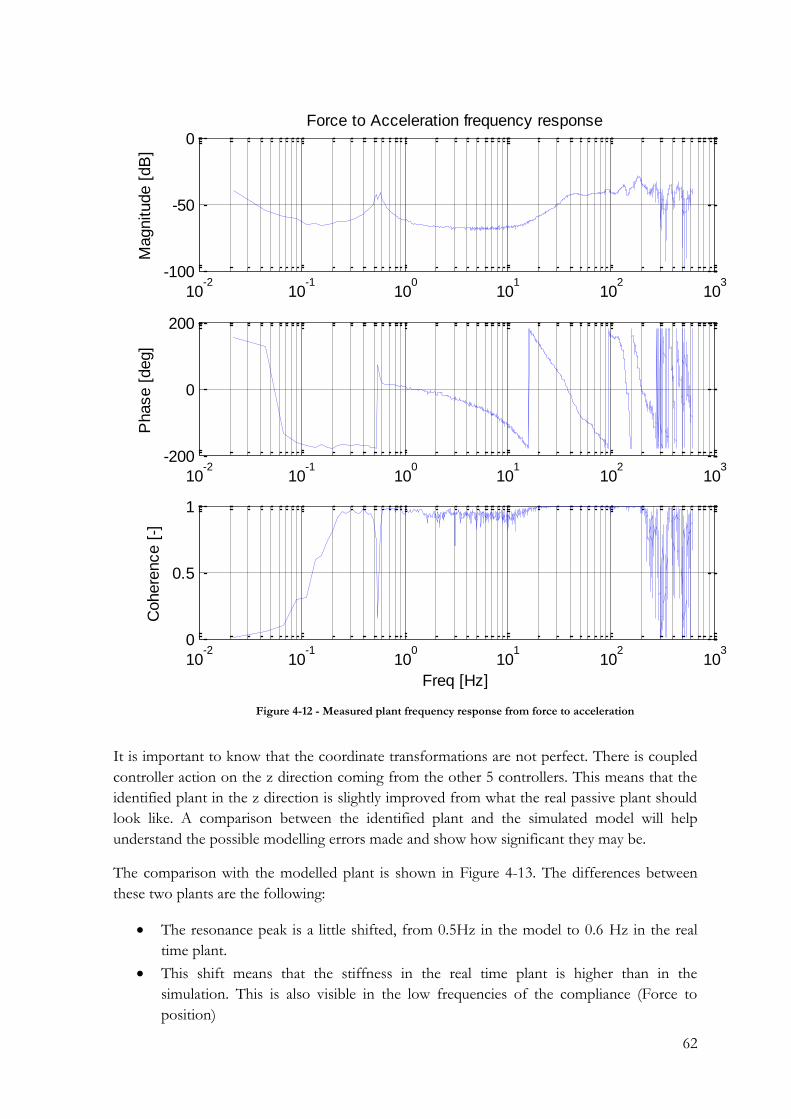
62
It is important to know that the coordinate transformations are not perfect. There is coupled
controller action on the z direction coming from the other 5 controllers. This means that the
identified plant in the z direction is slightly improved from what the real passive plant should
look like. A comparison between the identified plant and the simulated model will help
understand the possible modelling errors made and show how significant they may be.
The comparison with the modelled plant is shown in Figure 4-13. The differences between
these two plants are the following:
The resonance peak is a little shifted, from 0.5Hz in the model to 0.6 Hz in the real
time plant.
This shift means that the stiffness in the real time plant is higher than in the
simulation. This is also visible in the low frequencies of the compliance (Force to
position)
10-2
10-1
100
101
102
103
-100
-50
0M
agnitude [
dB
]
Force to Acceleration frequency response
10-2
10-1
100
101
102
103
-200
0
200
Phase [
deg]
10-2
10-1
100
101
102
103
0
0.5
1
Cohere
nce [
-]
Freq [Hz]
Figure 4-12 - Measured plant frequency response from force to acceleration

63
There is a big mass decoupling at around 40Hz that has not been modelled for the
simulation.
When comparing the phases it is apparent that they are very different. This is
problematic for the stability of the controlled system as the phase makes constant shits
of 360 degrees whereas in the simulation it keeps constant.
10-2
10-1
100
101
102
103
-250
-200
-150
-100
-50Force to Position
10-2
10-1
100
101
102
103
-120
-100
-80
-60
-40
-20Force to Acceleration
Modelled plant
Identified plant
Figure 4-13 - Modelled vs identified plant frequency response magnitude

64
4.3 Closed loop Finally the controllers have been set on the closed loop. The results are the following:
The frequency response of the manually shaped controller is shown in Figure 4-15. The
results show that the manually tuned controller does not improve on the open loop response.
Except at high frequencies, but the region of interest remains the same.
In the case of the H-infinity methods they both ended up being unstable. This is because the
methods are very dependent on the plant´s model and the used model is not all that accurate.
Figure 4-14 - Modelled vs identified plant frequency response phase
10-2
10-1
100
101
102
103
-200
-100
0
100
200Force to Position
10-2
10-1
100
101
102
103
-200
-100
0
100
200Force to Acceleration

65
10-2
10-1
100
101
102
103
104
-250
-200
-150
-100
-50Force to position
Open Loop
Closed Loop
10-2
10-1
100
101
102
103
104
-150
-100
-50
0
50Force to acceleration
Figure 4-15 - Manually tuned controller closed loop.

66
5 Conclusiones y trabajo futuro En la fase de diseño se crearon tres controladores mediante tres métodos distintos diseñados
para aumentar el aislamiento de un modelo simplificado a una sola dirección.
El método clásico debido a su naturaleza iterativa es exigente en el tuneado aunque finalmente
se obtuvo un buen rendimiento en el aislamiento de vibraciones.
El método de H-infinito básico se centraba en minimizar el movimiento de la masa a aislar. El
controlador obtenido mediante este método no mejora el rendimiento del aislamiento. Esto se
debe a la reducida cantidad de información sobre el modelo a aislar que se insertó en la planta
aumentada. La intención a partir de aquí era la de mejorar este método para reducir la cantidad
de estudio previo necesario para los métodos de H-infinito además de aumentar la relación
entre el método y las respuestas en frecuencia de la planta a aislar.
El método de H-infinito mejorado crea un controlador bajo la premisa de minimizar la
diferencia entre las respuestas en frecuencia del modelo y las respuestas en frecuencia
deseadas. El controlador obtenido obtiene un rendimiento parecido al obtenido mediante el
método clásico. Lo que se extrae de estos resultados es que el método creado se puede utilizar
para generar controladores con la misma confianza que los métodos clásicos con la ventaja de
que los métodos H-infinito son escalables a modelos más complejos sin añadir complejidad al
tuneado.
Una vez obtenidos los controladores en la simulación se procedió a probarlos en tiempo real
sobre un maquina física.
En el entorno real los controladores resultaron ser o inestables o no proporcionaban un
aislamiento mejorado. La razón por la que esto ocurre es que la diferencia que existe entre el
modelo simulado y la máquina física es mayor que el margen permitido para la incertidumbre.
Para poder comprobar si es posible crear controladores para las máquinas físicas es necesario
crear un modelo más preciso. Además en el estudio llevado a cabo no se añadió ninguna
información sobre incertidumbre. Para evitar las posibles inestabilidades es necesario estudiar
la incertidumbre de la máquina física para poder añadirla al diseño del controlador.
Trabajos futuros
Hay distintas vertientes que se pueden ser la continuación de este proyecto todas basadas en el
método de H-infinito basados en distintas características del método. Como son la posibilidad
de añadir conocimiento sobre la incertidumbre del modelo o la facilidad con la que se puede
escalar a modelos más complejos. También es aprovechable la capacidad de este tipo de
modelos de otorgar siempre controladores óptimos para estudiar otros aspectos que afectan
de forma paralela al aislamiento activo. Los temas que se podrían tratar son los siguientes.
Mejorar el método de H-infinito de modelado de respuestas en frecuencia añadiendo
conocimiento sobre la incertidumbre visto que esta información es necesaria para la
estabilidad de los sistemas controlados.

67
Expandir el modelo para diseñar controladores para modelos con seis grados de
libertad que se aproximen más a la máquina física
Es posible estudiar otras limitaciones al aislamiento activo como serían las
características de los acelerómetros (niveles de ruido, sensibilidad.)

68
5 Conclusions and future work The designing phase showed how it is possible to design a controller using optimal control
design methods that provide good isolation results. The obtained results for the optimal
controllers did not improve on the loop shaping method. However this is due to the simple
approach taken on the H-infinity methods where the information used to characterize the
plant was very little with only some characterization on the sensor noise and some
performance requirements.
In the test setup the designed controllers where set on a real machine. The designed
controllers turned out to be unstable or did not provide increased isolation. The reason for
this is that the margins given for divergences between the real plant and the simulation where
too small. That means that the controllers were not designed for the real machine and that
makes their behaviour unpredictable.
For further research if the controllers in the design phase want to be optimized more
information about the inputs and uncertainties of the machine should be studied. The study of
the uncertainties of the plant by identifying the plant is very important to avoid obtaining
controllers that end up being unstable.
The best way to design a controller through H-infinity methods is to start by making an
extensive study on the frequency characteristics of the plant that it is going to be applied to.
Of especial importance are obtaining a precise model of the plant as the H-infinity method is
so dependent on it and the uncertainty bounds which provide the so much needed robust
stability.
Once a good controller has been created for the 1DoF models it can be very interesting to
extend the methods to 6DoF models. Using the H-infinity method to create a controller for
6DOF should not be much harder than doing it for a 1DOF. And a single controller created
for 6DoF should also provide better results than those existing. This is because the couplings
between the coordinates of the machine would also be optimized within the H-infinity
algorithms.
69
6 Works Cited A.Joanknecht, H. (n.d.). Performance optimization of active vibration isolators using modern control
techniques.
C.Doyle, J., A.Francis, B., & R.Tannenbaum, A. (n.d.). Feedback control Theory. Macmillan.
Damen, A., & Weiland, S. (n.d.). Robust Control.
Ding, C., Damen, A., & Bosch, P. v. (2012). Robust Vibration Isolation by Frequency-Shaped Sliding
Surface Control with Floor Velocity/Acceleration Measurement.
Ding, C., Damen, A., Bosch, P. v., & Janssen, J. (n.d.). Vibration Isolation of an Electomagnetic
Actuator with Passive Gravity Compensation.
F.Franklin, G., Powell, J. D., & Emami-Naeini, A. (n.d.). Feedback Control of Fynamic Systems.
Addison Wesley.
Meirovithc, L. (2003). Fundamentals of Vibrations. McGrawHill.
Nakashima, K., Tsujino, T., & Fuji, T. (1996). Multivariable Control of a Magnetic Levitation
System Using Closed Loop Identificantion and H-infinity Control Theory. Conference on
Decision and Control. Kobe, Japan.
Nelson, P. G. (n.d.). (TMC) Retrieved June 2013, from
http://www.techmfg.com/techbkgd/techbkgd_5.html#figure17
Pantazi, A., Sebastian, A., Pozidis, H., & Eleftheriou, E. (2005). Two-sensor-based H-infiniti
control for nanopositioning in probe storage. European Control Conference. Seville, Spain.
Peña, R. S., & Sznaier, M. (n.d.). Robust Systems: Theory and Applications. Wiley.
Skogestad, S., & Postelwaith, I. (n.d.). Multivariable Feedback Control. Wiley.
Wal, M. v., & Heertjes, M. (n.d.). The effect of sensor selection on the achievable performance of vibration
isolators.
Watanabe, K., & al., e. (1996). Combination of H-infinity en PI Control for an
Electromechanically Levitated Vibration Isolation System. Conference on Decision and
Control. Kobe, Japan.
Yasuda, M., Osaka, T., & Ikeda, M. (1996). Feedforward Control of a Vibration Isolation
System for Disturbance Suppresion. Conference on Decision and Control. Kobe, Japan.
Zhou, K., & Doyle, J. C. (1999). Essentials of Robust Control. Prentice Hall.

70
7 PRESUPUESTO 1) Ejecución Material
Licencia Matlab....... ....................................................................................... 2.000 €
Sistema dSpace (RTI) .................................................................................... 10000 €
Ordenador ........................................................................................................ 1500 €
Componetes (sensores, cables etc…) ............................................................. 400 €
Total de ejecución material ......................................................................... 13900 €
2) Gastos generales
16 % sobre Ejecución Material .............................................................. 2224 €
3) Beneficio Industrial
6 % sobre Ejecución Material .................................................................. 834 €
4) Honorarios Proyecto
1500 horas a 15 € / hora ....................................................................... 22500 €
5) Material fungible
Gastos de impresión .................................................................................... 60 €
Encuadernación ......................................................................................... 200 €
6) Subtotal del presupuesto
Subtotal Presupuesto ............................................................................. 39718 €
7) I.V.A. aplicable
21% Subtotal Presupuesto ................................................................ 8340,78 €
8) Total presupuesto
Total Presupuesto ............................................................................. 48058,78 €
Madrid, Septiembre de 2013
El Ingeniero Jefe de Proyecto
Fdo.: Pablo Wildschut
Ingeniero Superior de Telecomunicación

8 PLIEGO DE CONDICIONES
Este documento contiene las condiciones legales que guiarán la realización, en este
proyecto, de un método de diseño de controladores. En lo que sigue, se supondrá que el
proyecto ha sido encargado por una empresa cliente a una empresa consultora con la finalidad
de realizar dicho sistema. Dicha empresa ha debido desarrollar una línea de investigación con
objeto de elaborar el proyecto. Esta línea de investigación, junto con el posterior desarrollo de
los programas está amparada por las condiciones particulares del siguiente pliego.
Supuesto que la utilización industrial de los métodos recogidos en el presente
proyecto ha sido decidida por parte de la empresa cliente o de otras, la obra a realizar se
regulará por las siguientes:
8.1 Condiciones generales
1. La modalidad de contratación será el concurso. La adjudicación se hará, por tanto, a la
proposición más favorable sin atender exclusivamente al valor económico, dependiendo de las
mayores garantías ofrecidas. La empresa que somete el proyecto a concurso se reserva el derecho
a declararlo desierto.
2. El montaje y mecanización completa de los equipos que intervengan será realizado
totalmente por la empresa licitadora.
3. En la oferta, se hará constar el precio total por el que se compromete a realizar la obra
y el tanto por ciento de baja que supone este precio en relación con un importe límite si este se
hubiera fijado.
4. La obra se realizará bajo la dirección técnica de un Ingeniero Superior de
Telecomunicación, auxiliado por el número de Ingenieros Técnicos y Programadores que se
estime preciso para el desarrollo de la misma.
5. Aparte del Ingeniero Director, el contratista tendrá derecho a contratar al resto del
personal, pudiendo ceder esta prerrogativa a favor del Ingeniero Director, quien no estará
obligado a aceptarla.
6. El contratista tiene derecho a sacar copias a su costa de los planos, pliego de
condiciones y presupuestos. El Ingeniero autor del proyecto autorizará con su firma las copias
solicitadas por el contratista después de confrontarlas.

72
7. Se abonará al contratista la obra que realmente ejecute con sujeción al proyecto que
sirvió de base para la contratación, a las modificaciones autorizadas por la superioridad o a las
órdenes que con arreglo a sus facultades le hayan comunicado por escrito al Ingeniero Director
de obras siempre que dicha obra se haya ajustado a los preceptos de los pliegos de condiciones,
con arreglo a los cuales, se harán las modificaciones y la valoración de las diversas unidades sin
que el importe total pueda exceder de los presupuestos aprobados. Por consiguiente, el número
de unidades que se consignan en el proyecto o en el presupuesto, no podrá servirle de
fundamento para entablar reclamaciones de ninguna clase, salvo en los casos de rescisión.
8. Tanto en las certificaciones de obras como en la liquidación final, se abonarán los
trabajos realizados por el contratista a los precios de ejecución material que figuran en el
presupuesto para cada unidad de la obra.
9. Si excepcionalmente se hubiera ejecutado algún trabajo que no se ajustase a las
condiciones de la contrata pero que sin embargo es admisible a juicio del Ingeniero Director de
obras, se dará conocimiento a la Dirección, proponiendo a la vez la rebaja de precios que el
Ingeniero estime justa y si la Dirección resolviera aceptar la obra, quedará el contratista obligado
a conformarse con la rebaja acordada.
10. Cuando se juzgue necesario emplear materiales o ejecutar obras que no figuren en el
presupuesto de la contrata, se evaluará su importe a los precios asignados a otras obras o
materiales análogos si los hubiere y cuando no, se discutirán entre el Ingeniero Director y el
contratista, sometiéndolos a la aprobación de la Dirección. Los nuevos precios convenidos por
uno u otro procedimiento, se sujetarán siempre al establecido en el punto anterior.
11. Cuando el contratista, con autorización del Ingeniero Director de obras, emplee
materiales de calidad más elevada o de mayores dimensiones de lo estipulado en el proyecto, o
sustituya una clase de fabricación por otra que tenga asignado mayor precio o ejecute con
mayores dimensiones cualquier otra parte de las obras, o en general, introduzca en ellas cualquier
modificación que sea beneficiosa a juicio del Ingeniero Director de obras, no tendrá derecho sin
embargo, sino a lo que le correspondería si hubiera realizado la obra con estricta sujeción a lo
proyectado y contratado.
12. Las cantidades calculadas para obras accesorias, aunque figuren por partida alzada en
el presupuesto final (general), no serán abonadas sino a los precios de la contrata, según las
condiciones de la misma y los proyectos particulares que para ellas se formen, o en su defecto,
por lo que resulte de su medición final.

73
13. El contratista queda obligado a abonar al Ingeniero autor del proyecto y director de
obras así como a los Ingenieros Técnicos, el importe de sus respectivos honorarios facultativos
por formación del proyecto, dirección técnica y administración en su caso, con arreglo a las
tarifas y honorarios vigentes.
14. Concluida la ejecución de la obra, será reconocida por el Ingeniero Director que a tal
efecto designe la empresa.
15. La garantía definitiva será del 4% del presupuesto y la provisional del 2%.
16. La forma de pago será por certificaciones mensuales de la obra ejecutada, de acuerdo
con los precios del presupuesto, deducida la baja si la hubiera.
17. La fecha de comienzo de las obras será a partir de los 15 días naturales del replanteo
oficial de las mismas y la definitiva, al año de haber ejecutado la provisional, procediéndose si no
existe reclamación alguna, a la reclamación de la fianza.
18. Si el contratista al efectuar el replanteo, observase algún error en el proyecto, deberá
comunicarlo en el plazo de quince días al Ingeniero Director de obras, pues transcurrido ese
plazo será responsable de la exactitud del proyecto.
19. El contratista está obligado a designar una persona responsable que se entenderá con
el Ingeniero Director de obras, o con el delegado que éste designe, para todo relacionado con
ella. Al ser el Ingeniero Director de obras el que interpreta el proyecto, el contratista deberá
consultarle cualquier duda que surja en su realización.
20. Durante la realización de la obra, se girarán visitas de inspección por personal
facultativo de la empresa cliente, para hacer las comprobaciones que se crean oportunas. Es
obligación del contratista, la conservación de la obra ya ejecutada hasta la recepción de la
misma, por lo que el deterioro parcial o total de ella, aunque sea por agentes atmosféricos u
otras causas, deberá ser reparado o reconstruido por su cuenta.
21. El contratista, deberá realizar la obra en el plazo mencionado a partir de la fecha del
contrato, incurriendo en multa, por retraso de la ejecución siempre que éste no sea debido a
causas de fuerza mayor. A la terminación de la obra, se hará una recepción provisional previo
reconocimiento y examen por la dirección técnica, el depositario de efectos, el interventor y el
jefe de servicio o un representante, estampando su conformidad el contratista.

74
22. Hecha la recepción provisional, se certificará al contratista el resto de la obra,
reservándose la administración el importe de los gastos de conservación de la misma hasta su
recepción definitiva y la fianza durante el tiempo señalado como plazo de garantía. La recepción
definitiva se hará en las mismas condiciones que la provisional, extendiéndose el acta
correspondiente. El Director Técnico propondrá a la Junta Económica la devolución de la fianza
al contratista de acuerdo con las condiciones económicas legales establecidas.
23. Las tarifas para la determinación de honorarios, reguladas por orden de la Presidencia
del Gobierno el 19 de Octubre de 1961, se aplicarán sobre el denominado en la actualidad
“Presupuesto de Ejecución de Contrata” y anteriormente llamado ”Presupuesto de Ejecución
Material” que hoy designa otro concepto.
8.2 Condiciones particulares
La empresa consultora, que ha desarrollado el presente proyecto, lo entregará a la
empresa cliente bajo las condiciones generales ya formuladas, debiendo añadirse las
siguientes condiciones particulares:
1. La propiedad intelectual de los procesos descritos y analizados en el presente trabajo,
pertenece por entero a la empresa consultora representada por el Ingeniero Director del
Proyecto.
2. La empresa consultora se reserva el derecho a la utilización total o parcial de los
resultados de la investigación realizada para desarrollar el siguiente proyecto, bien para su
publicación o bien para su uso en trabajos o proyectos posteriores, para la misma empresa cliente
o para otra.
3. Cualquier tipo de reproducción aparte de las reseñadas en las condiciones generales,
bien sea para uso particular de la empresa cliente, o para cualquier otra aplicación, contará con
autorización expresa y por escrito del Ingeniero Director del Proyecto, que actuará en
representación de la empresa consultora.
4. En la autorización se ha de hacer constar la aplicación a que se destinan sus
reproducciones así como su cantidad.

75
5. En todas las reproducciones se indicará su procedencia, explicitando el nombre del
proyecto, nombre del Ingeniero Director y de la empresa consultora.
6. Si el proyecto pasa la etapa de desarrollo, cualquier modificación que se realice sobre
él, deberá ser notificada al Ingeniero Director del Proyecto y a criterio de éste, la empresa
consultora decidirá aceptar o no la modificación propuesta.
7. Si la modificación se acepta, la empresa consultora se hará responsable al mismo nivel
que el proyecto inicial del que resulta el añadirla.
8. Si la modificación no es aceptada, por el contrario, la empresa consultora declinará
toda responsabilidad que se derive de la aplicación o influencia de la misma.
9. Si la empresa cliente decide desarrollar industrialmente uno o varios productos en los
que resulte parcial o totalmente aplicable el estudio de este proyecto, deberá comunicarlo a la
empresa consultora.
10. La empresa consultora no se responsabiliza de los efectos laterales que se puedan
producir en el momento en que se utilice la herramienta objeto del presente proyecto para la
realización de otras aplicaciones.
11. La empresa consultora tendrá prioridad respecto a otras en la elaboración de los
proyectos auxiliares que fuese necesario desarrollar para dicha aplicación industrial, siempre que
no haga explícita renuncia a este hecho. En este caso, deberá autorizar expresamente los
proyectos presentados por otros.
12. El Ingeniero Director del presente proyecto, será el responsable de la dirección de la
aplicación industrial siempre que la empresa consultora lo estime oportuno. En caso contrario, la
persona designada deberá contar con la autorización del mismo, quien delegará en él las
responsabilidades que ostente.


