Pumped thermal grid storage with heatexchange Cite as: J. Renewable Sustainable Energy 9, 044103 (2017); https://doi.org/10.1063/1.4994054Submitted: 03 July 2017 . Accepted: 05 July 2017 . Published Online: 02 August 2017
Robert B. Laughlin
COLLECTIONS
This paper was selected as Featured
ARTICLES YOU MAY BE INTERESTED IN
Nobel laureate brings in Brayton physics for inexpensive renewable energy storageScilight 2017, 060005 (2017); https://doi.org/10.1063/1.4996272
In search of the wind energy potentialJournal of Renewable and Sustainable Energy 9, 052301 (2017); https://doi.org/10.1063/1.4999514
Highly-efficient thermoelectronic conversion of solar energy and heat into electric powerJournal of Renewable and Sustainable Energy 5, 043127 (2013); https://doi.org/10.1063/1.4817730
Department of Physics, Stanford University, Stanford, California 94305, USA
(Received 3 July 2017; accepted 5 July 2017; published online 2 August 2017)
A thermal heat-pump grid storage technology is described based on closed-cycle
Brayton engine transfers of heat from a cryogenic storage fluid to molten solar salt.
Round-trip efficiency, computed as a function of turbomachinery polytropic efficiency
and total heat exchanger steel mass, is found to be competitive with that of pumped
hydroelectric storage. The cost per engine watt and cost per stored joule based are
estimated based on the present-day prices of power gas turbines and market prices of
steel and nitrate salt. Comparison is made with electrochemical and mechanical grid
storage technologies. VC 2017 Author(s). All article content, except where otherwisenoted, is licensed under a Creative Commons Attribution (CC BY) license (http://creativecommons.org/licenses/by/4.0/). [http://dx.doi.org/10.1063/1.4994054]
I. INTRODUCTION
It is widely understood that facilities for storing very large amounts of electric energy are
key to any long-term plan to supplant fossil fuel with renewable energy.1–3 The desirability of
switching to renewable sources is, of course, controversial, and it is not clear that eliminating
fossil fuel is economically feasible at this time.4–7 But without storage, it is also impossible.8
The intermittencies of energy sources like wind and sun are fundamentally incompatible with
the electricity industry’s need to supply power to customers—the instant demands by custom-
ers. The overriding importance of timing is demonstrated by the frequent development of nega-
tive spot prices for electric energy in markets with large wind deployments.9–12
The purpose of this paper is to discuss a specific storage technology and make the case
that it has the right engineering compromises to prevail when the need for storage eventually
becomes acute. It is an implementation of pumped thermal storage, an idea already in the litera-
ture and under development in industry, and differs from others chiefly in the substitution of
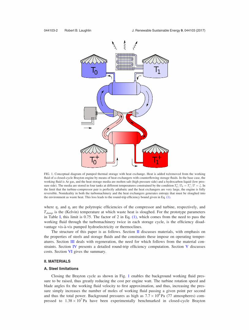
heat exchangers for thermoclines13–17 (Fig. 1). Instead of pumping water uphill from a low res-
ervoir to a higher one to store energy, as occurs in pumped hydroelectricity, one pumps heat
from a cold body to a hot one by means of a heat engine. In either case, the process is revers-
ible so that energy banked can be withdrawn later to satisfy demand.
The reasoning leading to the “Brayton Battery,” as it might be called, applies the metrics
of safety, low cost, and high efficiency, in this order. The average power delivered to a large
metropolitan area such as Los Angeles or New York is about 1.4� 1010 W.18 Storing this
power for only one hour gives 5.04� 1013 J or one Hiroshima-sized atomic bomb.19 It is abso-
lutely essential that explosive release of this stored energy be physically impossible. Once this
safety criterion is met, capital and maintenance costs must be brutally minimized, even at the
price of a small hit in round-trip efficiency, because storage of electricity is fundamentally
about value, not about conserving energy.
The round-trip storage efficiency gstore of the configuration in Fig. 1 satisfies
where gc and gt are the polytropic efficiencies of the compressor and turbine, respectively, and
Tdump is the (Kelvin) temperature at which waste heat is sloughed. For the prototype parameters
in Table I, this limit is 0.75. The factor of 2 in Eq. (1), which comes from the need to pass the
working fluid through the turbomachinery twice in each storage cycle, is the efficiency disad-
vantage vis-�a-vis pumped hydroelectricity or thermoclines.
The structure of this paper is as follows. Section II discusses materials, with emphasis on
the properties of steels and storage fluids and the constraints these impose on operating temper-
atures. Section III deals with regeneration, the need for which follows from the material con-
straints. Section IV presents a detailed round-trip efficiency computation. Section V discusses
costs. Section VI gives the summary.
II. MATERIALS
A. Steel limitations
Closing the Brayton cycle as shown in Fig. 1 enables the background working fluid pres-
sure to be raised, thus greatly reducing the cost per engine watt. The turbine rotation speed and
blade angles fix the working fluid velocity to first approximation, and thus, increasing the pres-
sure simply increases the number of moles of working fluid passing a given point per second
and thus the total power. Background pressures as high as 7.7� 106 Pa (77 atmospheres) com-
pressed to 1.38� 107 Pa have been experimentally benchmarked in closed-cycle Brayton
FIG. 1. Conceptual diagram of pumped thermal storage with heat exchange. Heat is added to/removed from the working
fluid of a closed-cycle Brayton engine by means of heat exchangers with counterflowing storage fluids. In the base case, the
working fluid is Ar gas, and the heat storage media are molten salt (high pressure side) and a hydrocarbon liquid (low pres-
sure side). The media are stored in four tanks at different temperatures constrained by the condition Tþ0 =T0 ¼ Tþ1 =T ¼ n. In
the limit that the turbine-compressor pair is perfectly adiabatic and the heat exchangers are very large, the engine is fully
reversible. Nonideality in both the turbomachinery and the heat exchangers generates entropy that must be sloughed into
the environment as waste heat. This loss leads to the round-trip efficiency bound given in Eq. (1).
044103-2 Robert B. Laughlin J. Renewable Sustainable Energy 9, 044103 (2017)
engines using supercritical CO2.20 Pressures approaching 3.0� 107 Pa (300 atm) are routine in
modern supercritical steam power plants.21
However, the use of high pressure severely limits the temperatures that one can employ.
As shown in Fig. 2, raising the temperature of a steel eventually causes it to exhibit creep, a
slow plastic deformation that presages full mechanical failure at higher temperatures. This
effect is irrelevant on short time scales but is a major design constraint on the scale of
40 years.22 Creep is what prevents conventional carbon steels from being used in high-pressure
thermal applications at temperatures above about 700 K (427 �C). This limit can be raised to
about 800 K (527 �C) by adding impurities in percent amounts that block grain boundary
motion, but maximum resistance to creep requires full alloying with Cr and Ni to make stain-
less steels.22 The creep limitations of alloy steels may be seen from Fig. 2 to apply universally,
including to Inconels. Thus, pressure vessels constructed from steel become problematic for
TABLE I. Prototype design parameters assumed throughout this paper. The differences between charge and discharge are
ignored for clarity, as is the need to make Tdump higher than ambient to slough heat effectively. The compressor polytropic
efficiency gc is the ratio of ideal compressive work to actual work in the limit of small compression (i.e., for a single stage).
The turbine polytropic efficiency gt is the inverse of this ratio in the limit of small expansion. These particular values gc
and gt are industry standards discussed further in Sec. IV B.59–63
Ar N2
T0 180 K 180 K
Tþ0 300 K 300 K
T1 495 K 495 K
Tþ1 823 K 823 K
Tdump 300 K 300 K
n 1.66 1.66
gc 0.91 0.91
gt 0.93 0.93
p0 1.00 � 105 Pa 1.00 � 105 Pa
pl 1.00 � 106 Pa 1.00 � 106 Pa
ph 3.55 � 106 Pa 6.52 � 105 Pa
FIG. 2. Maximum steel stress allowed by the 2007 ASME Boiler and Pressure Vessel Code, Part II, Section D, Tables 1A
and 1B for a representative selection of steels (seamless tubing).22 The “creep cliff” at T¼ 873 K (600 �C) is clearly visible.
Black: Carbon steels, UNS Nos. K01201, K02707, and K03501. Red: Low-alloy steels, UNS Nos. K11522, K11547,
K11597, and K21590. Blue: Stainless steels, UNS Nos. S30409, S30815, S31609, S32109, S34709, and N08810 (Incalloy
800H).
044103-3 Robert B. Laughlin J. Renewable Sustainable Energy 9, 044103 (2017)
temperatures much above 873 K (600 �C). This is a major consideration in present-day super-
critical steam plants.21
B. Solar salt
The temperature limitations of steels make solar salt, the elementary NaNO3/KNO3 eutectic
storage medium of the concentrating solar industry, to be a particularly good choice for the
high-temperature storage medium.23–25 All solid and liquid substances have heat capacities of
approximately 3R per mole of atoms, where R is the ideal gas constant, in the temperature
range of interest, so virtually, anything will act as a thermal storage medium, including rocks.
However, the cost of either gravel or salt is much less than the cost of the engine for storage
times less than 1 day, and salt has the great advantage of being liquid, thus enabling heat trans-
fer by counterflow, minimizing entropy creation. Solar salt has a well-known list of other
advantages such as low vapor pressure, high compatibility with steels, and environmental
friendliness. It does not disintegrate in response to thermal cycling stresses the way a solid
would. It creates no explosion hazard.
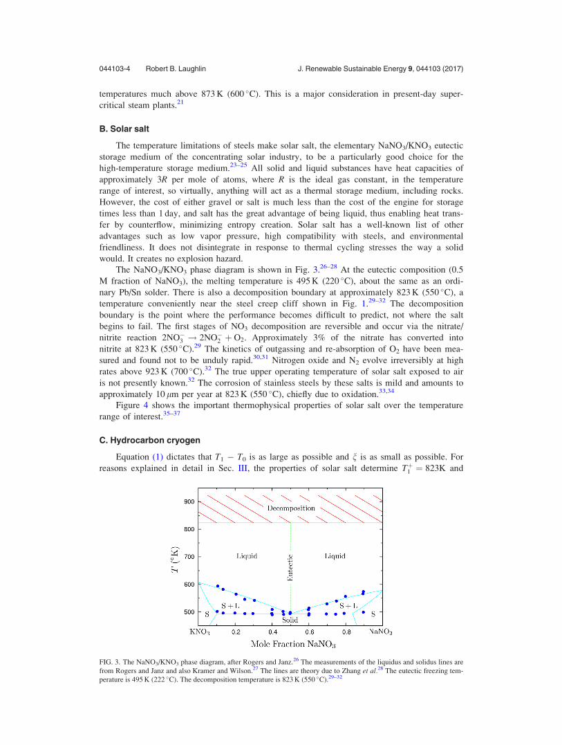
The NaNO3/KNO3 phase diagram is shown in Fig. 3.26–28 At the eutectic composition (0.5
M fraction of NaNO3), the melting temperature is 495 K (220 �C), about the same as an ordi-
nary Pb/Sn solder. There is also a decomposition boundary at approximately 823 K (550 �C), a
temperature conveniently near the steel creep cliff shown in Fig. 1.29–32 The decomposition
boundary is the point where the performance becomes difficult to predict, not where the salt
begins to fail. The first stages of NO3 decomposition are reversible and occur via the nitrate/
nitrite reaction 2NO�3 ! 2NO�2 þ O2. Approximately 3% of the nitrate has converted into
nitrite at 823 K (550 �C).29 The kinetics of outgassing and re-absorption of O2 have been mea-
sured and found not to be unduly rapid.30,31 Nitrogen oxide and N2 evolve irreversibly at high
rates above 923 K (700 �C).32 The true upper operating temperature of solar salt exposed to air
is not presently known.32 The corrosion of stainless steels by these salts is mild and amounts to
approximately 10 lm per year at 823 K (550 �C), chiefly due to oxidation.33,34
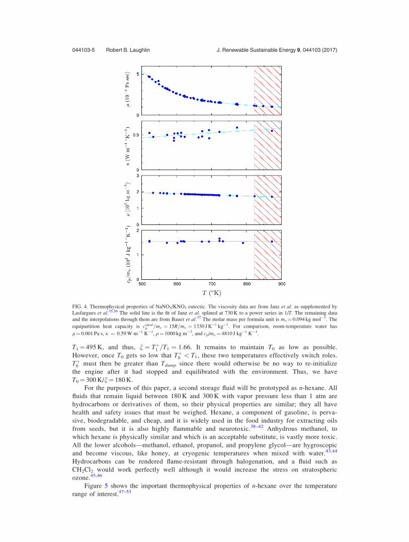
Figure 4 shows the important thermophysical properties of solar salt over the temperature
range of interest.35–37
C. Hydrocarbon cryogen
Equation (1) dictates that T1 � T0 is as large as possible and n is as small as possible. For
reasons explained in detail in Sec. III, the properties of solar salt determine Tþ1 ¼ 823K and
FIG. 3. The NaNO3/KNO3 phase diagram, after Rogers and Janz.26 The measurements of the liquidus and solidus lines are
from Rogers and Janz and also Kramer and Wilson.27 The lines are theory due to Zhang et al.28 The eutectic freezing tem-
perature is 495 K (222 �C). The decomposition temperature is 823 K (550 �C).29–32
044103-4 Robert B. Laughlin J. Renewable Sustainable Energy 9, 044103 (2017)
T1¼ 495 K, and thus, n ¼ Tþ1 =T1 ¼ 1:66. It remains to maintain T0 as low as possible.
However, once T0 gets so low that Tþ0 < T1, these two temperatures effectively switch roles.
Tþ0 must then be greater than Tdump since there would otherwise be no way to re-initialize
the engine after it had stopped and equilibrated with the environment. Thus, we have
T0¼ 300 K/n¼ 180 K.
For the purposes of this paper, a second storage fluid will be prototyped as n-hexane. All
fluids that remain liquid between 180 K and 300 K with vapor pressure less than 1 atm are
hydrocarbons or derivatives of them, so their physical properties are similar; they all have
health and safety issues that must be weighed. Hexane, a component of gasoline, is perva-
sive, biodegradable, and cheap, and it is widely used in the food industry for extracting oils
from seeds, but it is also highly flammable and neurotoxic.38–42 Anhydrous methanol, to
which hexane is physically similar and which is an acceptable substitute, is vastly more toxic.
All the lower alcohols—methanol, ethanol, propanol, and propylene glycol—are hygroscopic
and become viscous, like honey, at cryogenic temperatures when mixed with water.43,44
Hydrocarbons can be rendered flame-resistant through halogenation, and a fluid such as
CH2Cl2 would work perfectly well although it would increase the stress on stratospheric
ozone.45,46
Figure 5 shows the important thermophysical properties of n-hexane over the temperature
range of interest.47–53
FIG. 4. Thermophysical properties of NaNO3/KNO3 eutectic. The viscosity data are from Janz et al. as supplemented by
Lasfargues et al.35,36 The solid line is the fit of Janz et al. splined at 730 K to a power series in 1/T. The remaining data
and the interpolations through them are from Bauer et al.37 The molar mass per formula unit is m�¼ 0.094 kg mol�1. The
equipartition heat capacity is cidealp =m� ¼ 15R=m� ¼ 1330 J K�1 kg�1. For comparison, room-temperature water has
l¼ 0.001 Pa s, j ¼ 0.59 W m�1 K�1, q¼ 1000 kg m�3, and cp/m�¼ 4810 J kg�1 K�1.
044103-5 Robert B. Laughlin J. Renewable Sustainable Energy 9, 044103 (2017)
D. Working fluid
The working fluid in this application is limited to gases that are extremely stable at high
temperatures and far from liquefaction or solidification phase transitions at mildly cryogenic
ones. The mechanical advantages of working near a critical point are outweighed in this case
by danger of fluid raining or snowing out and damaging the turbine blades. This eliminates, in
particular, CO2, which has both liquefaction and freezing transitions in the range of 200–300 K.
These considerations plus requirements of chemical inertness, cheapness, and environmental
friendliness restrict the possibilities to Ar and N2. The advantages of a lowered compression
ratio and, potentially, higher adiabatic efficiency by using a gas with no internal degrees of
freedom point to Ar as the preferred choice. However, N2 has the advantage of requiring only
minor modifications of rotor and stator airfoil shapes already optimized for use in air-breathing
jet engines.54
Table II shows the thermophysical properties of Ar and N2 over the temperature and pres-
sure range of interest.53 Both gases are functionally ideal (and thus polytropic) except at the
lowest temperatures. The correct low-temperature equation of state must be used in fine-tuning
the turbomachinery, but the ideal equation of state is sufficient for making efficiency and cost
estimates.
FIG. 5. Thermophysical properties of n-hexane (C6H14). The melting and boiling temperatures at 1 atm are 179 K and
350 K, respectively. The data are from various sources in the literature.47–52 The lines are from the NIST standard reference
database.53 The temperature calibration of Giller and Drickamer has been adjusted 3% to agree with the accepted melting
temperature.49 The molar mass per formula unit is m�¼ 0.086 kg mol�1. The equipartition capacity with hydrogen motion
frozen is cidealp =m� ¼ 18R=m� ¼ 1740 J K�1 kg�1.
044103-6 Robert B. Laughlin J. Renewable Sustainable Energy 9, 044103 (2017)
III. REGENERATION
The practical material limitations described in Sec. II require Tþ0 < T1. As shown in
Fig. 6, this condition causes heat transfers on the high-pressure and low-pressure sides of the
circuit to overlap, thus eliminating the need to actually transfer heat to or from the storage
fluids over this temperature range. Instead, heat may simply be transferred directly from one
side of the circuit to the other through a gas-gas heat exchanger, referred to as a regenerator,
or a recuperator.58 In the limit that the entropy generation by the heat exchangers is zero,
regeneration has no effect at all on the round-trip efficiency but simply reduces the amount
of heat exchanger steel required. It also reduces the temperature ranges over which the stor-
age fluids are required to be liquid. A modified version of Fig. 1 with regeneration included
is shown in Fig. 7.
Figures 6 and 7 clarify why Tþ0 cannot exceed Tdump. An engine powered down and equili-
brated to Tdump could easily be re-initialized by heating the (frozen) solar salt from Tdump to T1,
but it could not be easily re-initialized if Tþ0 had to be cooled to a value less than Tdump.
Figure 6 justifies choosing T1 to be the solar salt melting point. With Tþ1 and Tþ0 fixed at
the solar salt decomposition temperature and ambient, respectively, Eq. (1) is maximized
when nlnðnÞ=n� 1Þ is minimized. However, it may be seen from the plot of this function in
Fig. 8 that the minimum occurs when n ! 1. Other costs not included in the calculation run
away in this limit, so the specific value n¼ 1 is not meaningful. However, the convergence of
the function itself to 1 in this limit has an important implication that there is no significant
round-trip efficiency penalty for 1< n< 2. Virtually, any value of n in this range will do.
Moreover, lowering T1 degrades the efficiency rather than improving it. There is thus no effi-
ciency advantage in employing specialty salts with lower melting temperatures.
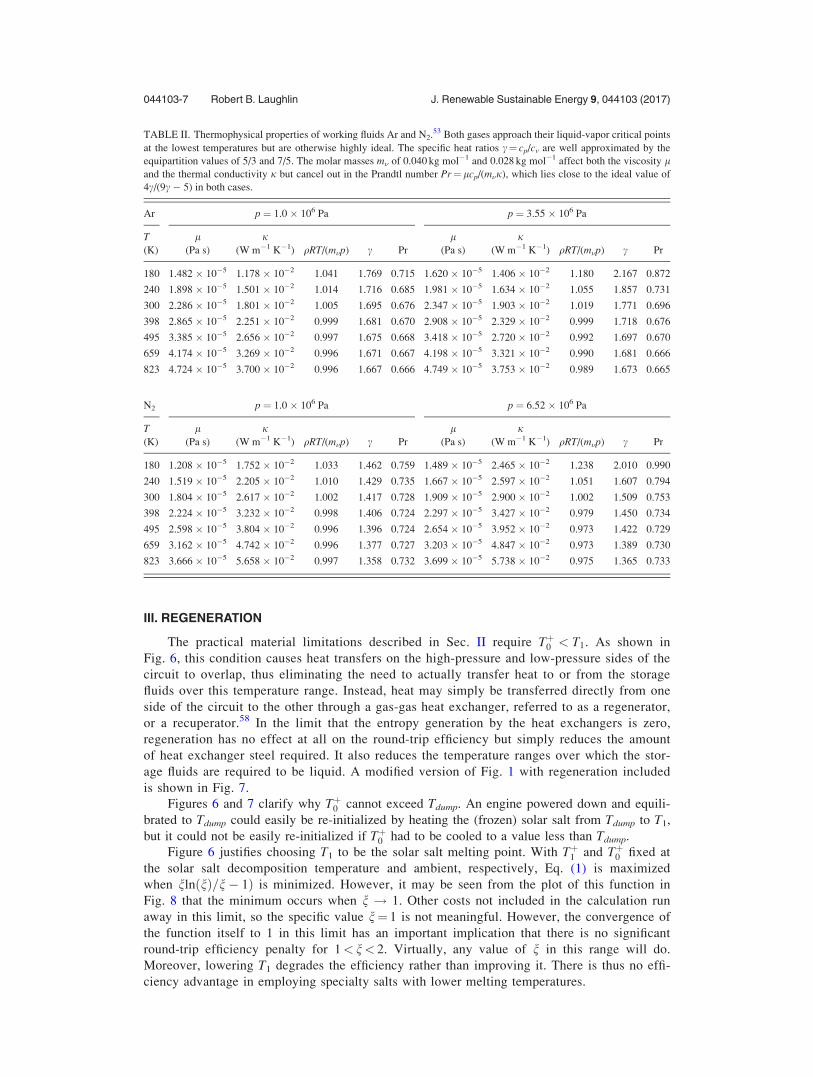
TABLE II. Thermophysical properties of working fluids Ar and N2.53 Both gases approach their liquid-vapor critical points
at the lowest temperatures but are otherwise highly ideal. The specific heat ratios c¼ cp/cv are well approximated by the
equipartition values of 5/3 and 7/5. The molar masses m� of 0.040 kg mol�1 and 0.028 kg mol�1 affect both the viscosity land the thermal conductivity j but cancel out in the Prandtl number Pr¼lcp/(m�j), which lies close to the ideal value of
4c/(9c � 5) in both cases.
Ar p ¼ 1.0 � 106 Pa p ¼ 3.55 � 106 Pa
T l jqRT/(m�p) c Pr
l jqRT/(m�p) c Pr(K) (Pa s) (W m�1 K�1) (Pa s) (W m�1 K�1)
044103-7 Robert B. Laughlin J. Renewable Sustainable Energy 9, 044103 (2017)
IV. ROUND-TRIP EFFICIENCY
A. Fictive temperature
The round-trip storage efficiency gstore is most simply computed through the entropy bud-
get. The system entropy S must be the same before and after a storage cycle because it is a
property of state, so any entropy DS generated during the cycle must be discarded as waste
heat TdumpDS, where Tdump is the slough temperature, roughly ambient. This heat represents a
loss from the stored energy Estore that cannot be re-transmitted as grid power. We thus have
gstore < 1� Tdump
Tf
1
Tf¼ DS
Estore
� �: (2)
The main contributions to the fictive temperature Tf come from the turbomachinery and three
heat exchangers,
1
Tf¼ 1
Tturbof
þX 1
Thxf
: (3)
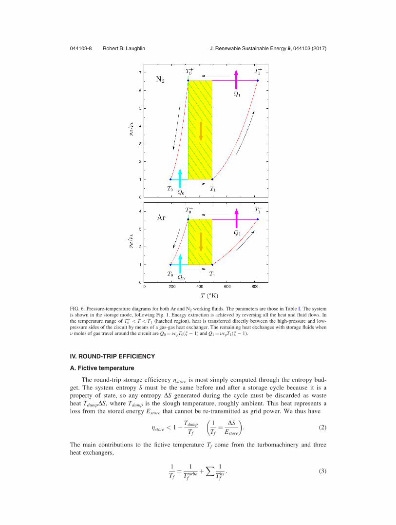
FIG. 6. Pressure-temperature diagrams for both Ar and N2 working fluids. The parameters are those in Table I. The system
is shown in the storage mode, following Fig. 1. Energy extraction is achieved by reversing all the heat and fluid flows. In
the temperature range of Tþ0 < T < T1 (hatched region), heat is transferred directly between the high-pressure and low-
pressure sides of the circuit by means of a gas-gas heat exchanger. The remaining heat exchanges with storage fluids when
� moles of gas travel around the circuit are Q0¼ �cpT0(n � 1) and Q1¼ �cpT1(n � 1).
044103-8 Robert B. Laughlin J. Renewable Sustainable Energy 9, 044103 (2017)
Other losses such as generator/motor inefficiency, unmanaged turbulence, and viscous drag in
the conduits are percent-level corrections.
B. Turbomachinery
In an adiabatic (entropy-conserving) compression or expansion, the temperature change dTresulting from a pressure change dp satisfies
dT
T¼ c� 1
c
� �dp
p; (4)
FIG. 7. Diagram of pumped thermal storage with heat exchange and regeneration. It is conceptually the same as Fig. 1 but
has T1 and Tþ0 reversed. The heat flows are as shown in Fig. 6.
FIG. 8. Plot of the merit function nlnðnÞ=ðn� 1Þ implicit in Eq. (1) with the values of Tþ0 and Tþ1 held fixed. The two circles cor-
respond to n¼ 823 K/495 K¼ 1.66 and n¼ 823 K/300 K¼ 2.74. This shows that NaNO3/KNO3 eutectic is nearly optimal as a
storage medium and that round-trip efficiency is actually degraded by the substitution of specialty salts with lower melting points.
044103-9 Robert B. Laughlin J. Renewable Sustainable Energy 9, 044103 (2017)
where c¼ cp/cv. In the limit that the turbomachinery is perfectly adiabatic, the temperature ratio
n in Fig. 1 is thus related to the ratio of the upper and lower pressures ph/pl by
n ¼ Tþ0 =T0 ¼ Tþ1 =T1 ¼ph
pl
� � c�1ð Þ=c: (5)
In a real turbocompressor, Eq. (4) is modified to
dT
T¼ 1
gc
c� 1
c
� �dp
p; (6)
where gc is the compressor polytropic efficiency. This slightly elevates the discharge tempera-
ture with respect to the ideal one for a given compression ratio. Integrating between the ideal
temperature and the actual one at a constant pressure gives the entropy created when � moles
of gas pass through the compressor
DSc ¼ð�cp
TdT ¼ �cp
1
gc
� 1
� �ln nð Þ: (7)
From the version of Eq. (6) appropriate for the turbine
dT
T¼ gt
c� 1
c
� �dp
p; (8)
one obtains similar entropy created when � moles of gas expand through the turbine
DSt ¼ð�cp
TdT ¼ �cp 1� gtð Þln nð Þ: (9)
Since the energy stored by cycling � moles of gas is Estore ¼ ðT1 � T0Þðn� 1Þ�cp, the inverse
fictive temperature of the turbomachinery is
1
Tturbof
¼ 2 DSc þ DStð ÞEstore
¼ 2
T1 � T0
1
gc
� gt
� �ln nð Þn� 1
: (10)
The factor of 2 accounts for summing the entropy generated during the storage and extraction
steps. Equation (1) is obtained by substituting this expression into Eq. (2).
The parameters of Table I give
Tturbof ¼ 1210 K: (11)
The values of gc and gt leading to this result lie at the extreme high end of present-day gas tur-
bine technology.59–63 They are benchmarked in the GE 90 aircraft engine. They are not charac-
teristics of turbomachinery generally, however, so custom design is required to achieve them in
practice. Turbomachinery bought off the shelf is a product fine-tuned to specific market needs
that require a different set of compromises. There are theoretical indications that each gc and gt
could be improved a further 1%.64–67
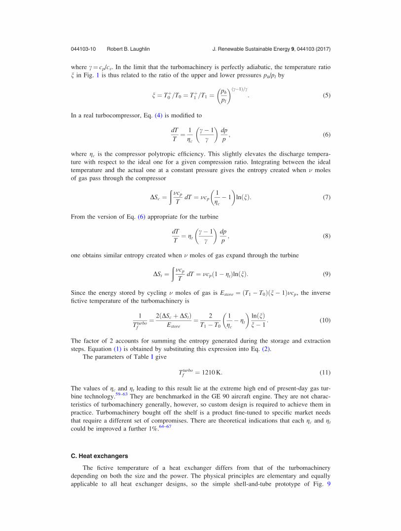
C. Heat exchangers
The fictive temperature of a heat exchanger differs from that of the turbomachinery
depending on both the size and the power. The physical principles are elementary and equally
applicable to all heat exchanger designs, so the simple shell-and-tube prototype of Fig. 9
044103-10 Robert B. Laughlin J. Renewable Sustainable Energy 9, 044103 (2017)
suffices for estimating the amount of steel required to achieve a given fictive temperature, even
if more advanced designs are actually employed.70,71
The laminar and turbulent cases are both important. The Reynolds number inside a heat
exchanger tube is
Re ¼ 2
Npa
m� _�
l
� �; (12)
where a is the tube’s inner radius, N is the number of tubes, and _� is the number of moles of
working fluid passing through the circuit per unit time. The flow is laminar if Re< 2000, turbu-
lent if Re> 3000, and intermittent otherwise. For this particular application, the effects of tur-
bulence are adequately accounted for by replacing l and j in the laminar expressions by the
Darcy-Weisbach formula55,56
~l ¼ lRe
64
� �f
� �(13)
with the Swamee-Jain approximation for the Darcy friction factor
f ¼ 0:25 log10
�
7:4aþ 5:74
Re0:9
� �� ��2
(14)
and the Gnielinski correlation
~j ¼ j11
48
� �f=8ð Þ Re� 1000ð ÞPr
1:0þ 12:7 f=8ð Þ1=2 Pr2=3 � 1ð Þ
" #; (15)
where Pr¼ lcp/(m�j) is the Prandtl number. Figure 10 shows these modifications to l and jfor various values of the tube surface roughness parameter �.
The laminar case follows from elementary considerations. Assuming a pressure gradient
@p/@z along the tube and solving the Navier-Stokes equation
l@2
@r2þ 1
r
@
@r
� �vz ¼
@p
@z(16)
FIG. 9. Illustration of the shell-and-tube prototype for the heat exchanger. The number of tubes shown is N¼ 151. The
lower right shows the case of b/a¼ 1.224 and d/b¼ 1.25. The lower left shows the case of b/a¼ 1.491.
044103-11 Robert B. Laughlin J. Renewable Sustainable Energy 9, 044103 (2017)
with a no-slip boundary condition, one obtains Hagen-Poiseuille flow
vz ¼1
4l@p
@z
� �r2 � a2ð Þ (17)
and an entropy generation due to viscous drag inside the tubes of
_Sinð Þ
visc ¼ �2pN
T
ða
0
@p
@z
� �vz rdr ¼ 8l
pa4
� �TL
N
R _�
p
� �2
: (18)
Assuming a temperature gradient @T/@z along the tube and similarly solving the heat flow
equation
j@2
@r2þ 1
r
@
@r
� �dT ¼ cp
p
RT
� �@T
@z
� �vz; (19)
one obtains the Graetz solution
dT ¼ 1
j@T
@z
� �cp _�
N
� �r2 r2 � 4a2 þ 3a4ð Þ
8pa4(20)
from which the entropy generation due to the thermal resistance inside the tubes is computed to be
_Sinð Þ
therm ¼ �2pjNL
T2
ða
0
@ dTð Þ@r
� �2
rdr
¼ 11
48pjL
N
� �@T
@z
� �cp _�
T
� �2
:
(21)
These two contributions to _SðinÞ
become equal when the heat exchanger length is L0, defined by
ffiffiffiffiffiffiffiffi384
11
r‘L0
a2¼ c
c� 1
� �DT
T; (22)
FIG. 10. Plot of turbulent enhancements of l and j defined by Eqs. (13) and (15) for Pr¼ 2/3 and surface roughness values
�/(2a)¼ 0.00, 0.01, 0.02, 0.03, 0.04, and 0.05.
044103-12 Robert B. Laughlin J. Renewable Sustainable Energy 9, 044103 (2017)
where DT is the temperature difference between the two ends of the heat exchanger and
‘ ¼ffiffiffiffiffiffiffiffiffijlTp
p(23)
is the working fluid scattering mean free path.57 The entropy creation outside the tube is a mul-
tiple of _SðinÞ
obtained by solving Eqs. (16) and (19) numerically for a given value of d. The
result is summarized in Table III. The fictive temperature is then
1
Thxf
¼ 11
24pjDT
T
1
T1 � T0ð Þ n� 1ð Þ
� �2
1þ_S
outð Þ
_Sinð Þ
" #1þ L2
L20
!_E
NL; (24)
where _E is the engine power. The factor of 2 accounts for entropy creation during both the stor-
age and extraction steps. Entropy creation due to heat flow in the steel is too small to matter in
this application.
There is no need to make the heat exchanger fictive temperature more than about 30 times
Tturbof . A set of parameters that give Thx
f in this range for laminar flow is shown Table III. The
important quantity for costing purposes is the steel mass per engine watt
M_E¼ qsteel p b2 � a2ð ÞL N
_E
� �: (25)
Here, N= _E is the number of tubes per engine watt, given by
N_E¼ 2
pa Re
m�
cpl
� �1
T1 � T0ð Þ n� 1ð Þ (26)
per Eq. (12). Both M= _E and Thxf remain unchanged if L is made smaller by keeping NL fixed
(which requires lowering Re). Thus, Table III actually describes a family of designs with differ-
ent aspect ratios but with similar performance characteristics.
Making L longer and keeping NL fixed push Re over the turbulence threshold. As shown in
Table IV, this causes a 50% reduction in M= _E for the same value of Tf. This occurs because
the turbulent enhancement of the thermal conductivity matters more than the turbulent enhance-
ment of the viscosity when L<L0. Thus, the optimal design with respect to steel mass has Rejust above the turbulence threshold. Further, cost compromise at this value of Re may result in
shortening of L keeping N fixed, reducing both Tf and M= _E proportionately.
The choice of tube inner and outer radii a and b has no effect on Tf if Re and L are held
fixed (and if L<L0), but it has a large effect on M= _E. Accordingly, the total cost of steel is
minimized by making a as small as possible. The minimum value of b/a required for creep
resistance is determined by
b2 � a2
b2 þ a2� Dp
rmax; (27)
where Dp is the pressure difference between the inside and outside of the tube and rmax is the
maximum stress allowed in the tube steel, shown in Fig. 2. To this minimal, b/a must be added
a mill tolerance margin, the default for which is a factor of 1.25 (12.5% of diameter), and a
salt corrosion margin, which is 4.0� 10�4 m for a 40-year lifespan.68,69 Thus, it is impractical
to make a much smaller than 1.5� 10�3 m in the high-temperature heat exchanger. The regen-
erator and low-temperature heat exchanger may involve microchannel designs of
a¼ 5.0� 10�4 m, thus potentially lowering M= _E in those cases.70,71
V. COST
The cost C of grid storage has two distinct metrics: the cost per engine watt @C=@ _E and the
cost per stored joule @C=@E. The first is characteristic of the engine and depends only on how
044103-13 Robert B. Laughlin J. Renewable Sustainable Energy 9, 044103 (2017)
fast energy is transferred to and from the grid, not on how much energy is stored or for how
long. The second characterizes the storage medium and is completely independent of how fast
energy is transferred in or out. One imagines first building the engine at a certain power rating
(and cost) and then adding as much storage capacity as circumstances warrant.
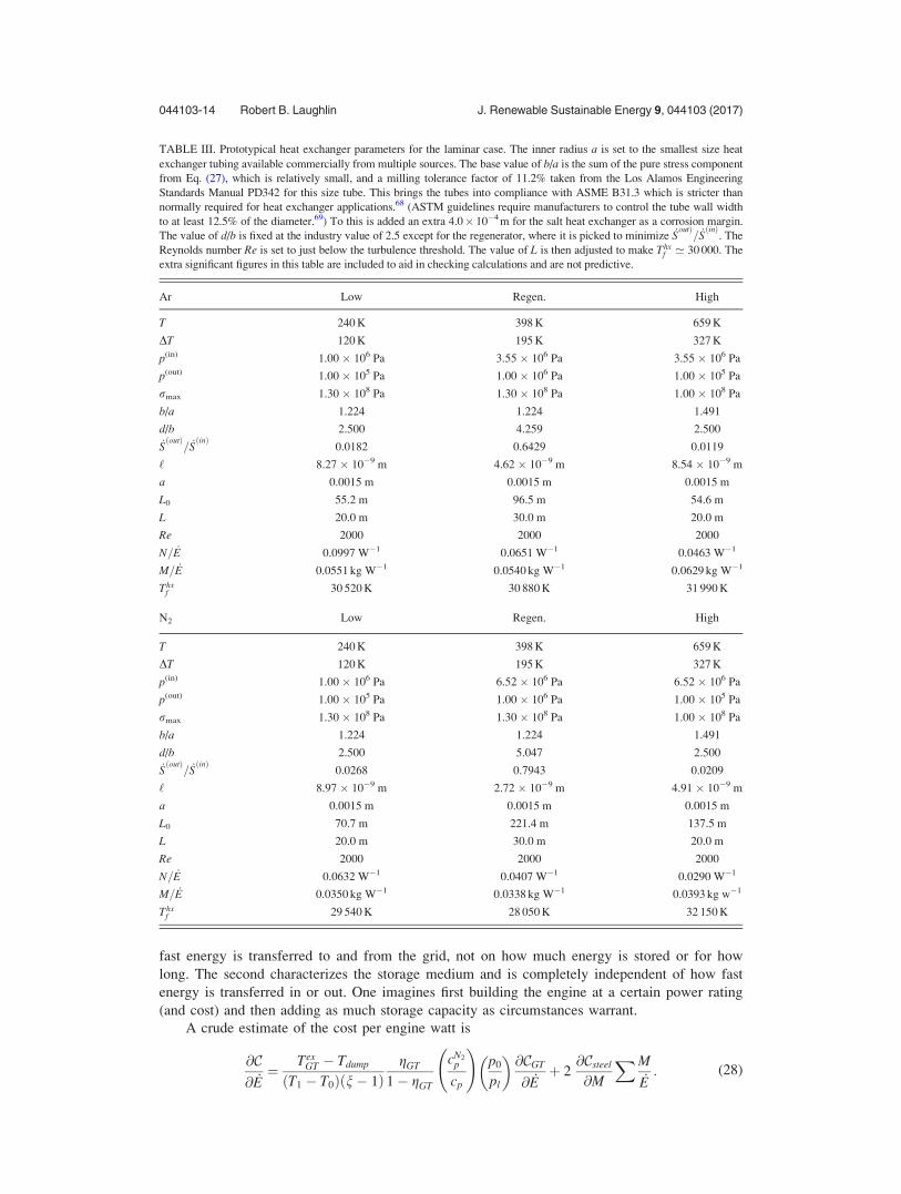
A crude estimate of the cost per engine watt is
@C@ _E¼ Tex
GT � Tdump
T1 � T0ð Þ n� 1ð ÞgGT
1� gGT
cN2p
cp
!p0
pl
� �@CGT
@ _Eþ 2
@Csteel
@M
XM_E: (28)
TABLE III. Prototypical heat exchanger parameters for the laminar case. The inner radius a is set to the smallest size heat
exchanger tubing available commercially from multiple sources. The base value of b/a is the sum of the pure stress component
from Eq. (27), which is relatively small, and a milling tolerance factor of 11.2% taken from the Los Alamos Engineering
Standards Manual PD342 for this size tube. This brings the tubes into compliance with ASME B31.3 which is stricter than
normally required for heat exchanger applications.68 (ASTM guidelines require manufacturers to control the tube wall width
to at least 12.5% of the diameter.69) To this is added an extra 4.0� 10�4 m for the salt heat exchanger as a corrosion margin.
The value of d/b is fixed at the industry value of 2.5 except for the regenerator, where it is picked to minimize _SoutÞ= _SðinÞ
. The
Reynolds number Re is set to just below the turbulence threshold. The value of L is then adjusted to make Thxf ’ 30 000. The
extra significant figures in this table are included to aid in checking calculations and are not predictive.
Ar Low Regen. High
T 240 K 398 K 659 K
DT 120 K 195 K 327 K
p(in) 1.00 � 106 Pa 3.55 � 106 Pa 3.55 � 106 Pa
p(out) 1.00 � 105 Pa 1.00 � 106 Pa 1.00 � 105 Pa
rmax 1.30 � 108 Pa 1.30 � 108 Pa 1.00 � 108 Pa
b/a 1.224 1.224 1.491
d/b 2.500 4.259 2.500
_SðoutÞ
= _SðinÞ
0.0182 0.6429 0.0119
‘ 8.27 � 10�9 m 4.62 � 10�9 m 8.54 � 10�9 m
a 0.0015 m 0.0015 m 0.0015 m
L0 55.2 m 96.5 m 54.6 m
L 20.0 m 30.0 m 20.0 m
Re 2000 2000 2000
N= _E 0.0997 W�1 0.0651 W�1 0.0463 W�1
M= _E 0.0551 kg W�1 0.0540 kg W�1 0.0629 kg W�1
Thxf 30 520 K 30 880 K 31 990 K
N2 Low Regen. High
T 240 K 398 K 659 K
DT 120 K 195 K 327 K
p(in) 1.00 � 106 Pa 6.52 � 106 Pa 6.52 � 106 Pa
p(out) 1.00 � 105 Pa 1.00 � 106 Pa 1.00 � 105 Pa
rmax 1.30 � 108 Pa 1.30 � 108 Pa 1.00 � 108 Pa
b/a 1.224 1.224 1.491
d/b 2.500 5.047 2.500
_SðoutÞ
= _SðinÞ
0.0268 0.7943 0.0209
‘ 8.97 � 10�9 m 2.72 � 10�9 m 4.91 � 10�9 m
a 0.0015 m 0.0015 m 0.0015 m
L0 70.7 m 221.4 m 137.5 m
L 20.0 m 30.0 m 20.0 m
Re 2000 2000 2000
N= _E 0.0632 W�1 0.0407 W�1 0.0290 W�1
M= _E 0.0350 kg W�1 0.0338 kg W�1 0.0393 kg w�1
Thxf 29 540 K 28 050 K 32 150 K
044103-14 Robert B. Laughlin J. Renewable Sustainable Energy 9, 044103 (2017)
The definitions of these parameters and their values are summarized in Tables I
and V.72–77 The idea behind this expression is that the turbomachinery should cost about the
same as a present-day commercial gas turbine of the same size. Thus, one scales the present-
day gas turbine cost by the number of moles per second _� required to give the given power.
The marginal cost of the (very large) heat exchangers required is estimated at 2 times the cost
of the steel used to make them. This is unrealistically low in the context of present-day heat
exchanger markets, but it is a reasonable expectation for large-volume production. This is con-
sistent with $2 kg�1 implicit in the heat-exchanger price figures in the study by Loh et al.,assuming a tube width of 0.125 times the tube diameter, the standard ASME milling margin.78
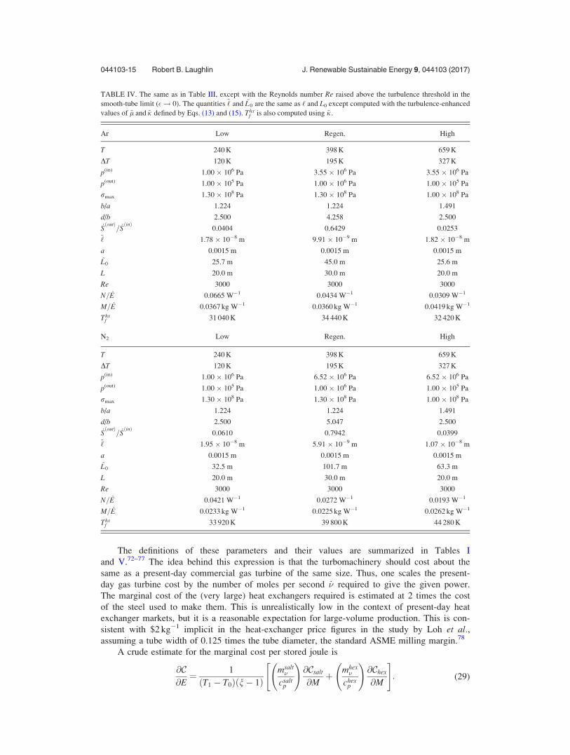
A crude estimate for the marginal cost per stored joule is
@C@E¼ 1
T1 � T0ð Þ n� 1ð Þmsalt�
csaltp
!@Csalt
@Mþ mhex
�
chexp
!@Chex
@M
" #: (29)
TABLE IV. The same as in Table III, except with the Reynolds number Re raised above the turbulence threshold in the
smooth-tube limit (�! 0). The quantities ~‘ and ~L0 are the same as ‘ and L0 except computed with the turbulence-enhanced
values of ~l and ~j defined by Eqs. (13) and (15). Thxf is also computed using ~j.
Ar Low Regen. High
T 240 K 398 K 659 K
DT 120 K 195 K 327 K
p(in) 1.00 � 106 Pa 3.55 � 106 Pa 3.55 � 106 Pa
p(out) 1.00 � 105 Pa 1.00 � 106 Pa 1.00 � 105 Pa
rmax 1.30 � 108 Pa 1.30 � 108 Pa 1.00 � 108 Pa
b/a 1.224 1.224 1.491
d/b 2.500 4.258 2.500
_SðoutÞ
= _SðinÞ
0.0404 0.6429 0.0253
~‘ 1.78 � 10�8 m 9.91 � 10�9 m 1.82 � 10�8 m
a 0.0015 m 0.0015 m 0.0015 m
~L0 25.7 m 45.0 m 25.6 m
L 20.0 m 30.0 m 20.0 m
Re 3000 3000 3000
N= _E 0.0665 W�1 0.0434 W�1 0.0309 W�1
M= _E 0.0367 kg W�1 0.0360 kg W�1 0.0419 kg W�1
Thxf 31 040 K 34 440 K 32 420 K
N2 Low Regen. High
T 240 K 398 K 659 K
DT 120 K 195 K 327 K
p(in) 1.00 � 106 Pa 6.52 � 106 Pa 6.52 � 106 Pa
p(out) 1.00 � 105 Pa 1.00 � 106 Pa 1.00 � 105 Pa
rmax 1.30 � 108 Pa 1.30 � 108 Pa 1.00 � 108 Pa
b/a 1.224 1.224 1.491
d/b 2.500 5.047 2.500
_SðoutÞ
= _SðinÞ
0.0610 0.7942 0.0399
~‘ 1.95 � 10�8 m 5.91 � 10�9 m 1.07 � 10�8 m
a 0.0015 m 0.0015 m 0.0015 m
~L0 32.5 m 101.7 m 63.3 m
L 20.0 m 30.0 m 20.0 m
Re 3000 3000 3000
N= _E 0.0421 W�1 0.0272 W�1 0.0193 W�1
M= _E 0.0233 kg W�1 0.0225 kg W�1 0.0262 kg W�1
Thxf 33 920 K 39 800 K 44 280 K
044103-15 Robert B. Laughlin J. Renewable Sustainable Energy 9, 044103 (2017)
The definitions of these parameters and their values are summarized in Tables I and V. The
idea behind this expression is that the asymptotic cost per stored joule is simply the cost of the
medium in which it is stored. Specifically omitted from this estimate because they are too small
to matter are the costs of large storage tanks ($50 m�3) and excavation ($2.4 m�3).78–80
Equations (28) and (29) are oversimplified, and they leave out many obvious costs—flow
handling, cooling structures, tanks, insulation, pumps, site preparation, and small loss account-
ing. However, they are sufficiently accurate to reveal the broad-brush picture: the cost of the
turbomachinery is lowered by the elevated pressure in the closed Brayton loop so much that the
cost per engine watt becomes dominated by the cost of the heat exchangers. The latter are con-
ceptually trivial and scale up easily to arbitrarily large sizes. They become arbitrarily efficient
when they do. Heat exchangers large enough to contribute negligibly to the total entropy budget
can be built for a total cost per engine watt comparable to that of a present-day simple-cycle
gas turbine. The marginal cost per stored joule, dominated by the cost of the storage fluids, is
about $3.54� 10�6 J�1 ($12.7 per kWh).
The plant cost curves associated with Table V are shown in Fig. 11. With the understand-
ing that these are only illustrations, on account of the large error bars, one can see that the cost
TABLE V. Top: Parameters used in Eq. (28) to estimate the cost per engine watt @C=@ _E. The total fictive temperature Tf is
computed with Eq. (3) using values in Table IV. The total mass per engine wattP
M= _E is obtained by summing the values
in Table IV. The standard gas turbine exhaust temperature TexGT and thermodynamic efficiency gGT are from Brooks.72 The
gas turbine cost per engine watt @CGT= _E is from Black and Veach, as reported by NREL.73 The Black and Veach cost of
0.60 W�1 for a simple cycle power plant upon which this estimate is based also agrees with Tidball et al.74 The cited steel
tubing price per kilogram @C/@M is on the extreme low edge of the market range. Fenton quotes $0.6 kg�1 as the carbon
steel price.75 The price of stainless steel is typically 5 times the price of carbon steel. Bottom: Parameters used in Eq. (29)
to estimate the marginal cost per stored joule @C=@E. The nitrate eutectic cost per kilogram @Csalt=@M is from Apodaca.76
The hexane cost per kilogram @Chex=@M is taken to be the price of gasoline reported by the U.S. EIA.77
Ar N2
Tf 1089 K 1107 KPM= _E 0.1136 kg W�1 0.0720 kg W�1
TexGT 873 K 823 K
gGT 0.38 0.038
@CGT=@ _E $0.25 W�1 $0.25 W�1
@Csteel=@M $1.00 kg�1 $1.00 kg�1
@C=@ _E $0.27 W�1 $0.20 W�1
@Csalt=@M $0.61 kg�1 $0.61 kg�1
@Chex=@M $0.70 kg�1 $0.70 kg�1
@C=@E $3.54 � 10�6 J�1 $3.54 � 10�6 J�1
FIG. 11. Cost structure implicit in Table V. This should be understood as an illustration only because the error bars of
Table V are very large. The base costs per engine watt @C=@ _E for Ar and N2 correspond to the two solid line intercepts at 0
h of storage time. The upper line is Ar. The slopes of these lines correspond to the marginal cost per stored joule @C=@E.
The dashed lines represent these quantities with $0.35 W�1 of infrastructure cost added (baffles, tanks, switchyard, build-
ings, etc.), the value needed to convert a $0.24 W�1 gas turbine into a full $0.6 W�1 simple-cycle power plant.73,74
044103-16 Robert B. Laughlin J. Renewable Sustainable Energy 9, 044103 (2017)
of the storage is negligible for storage times less than a day and thus that only the costs per
engine watt and plant infrastructure matter. There is, in particular, no significant economic
advantage in substituting rocks for solar salt and hexane.
VI. DISCUSSION
A. Physical constraints
Which storage technology actually prevails in the end will depend ultimately on cost, and
this is something difficult to assess correctly without actually building machines and testing
them. Thus, it is not possible to make a purely economic case that the technology described
here, which exists only as a concept, will win out. Rather the argument rests partly on such
cost analysis as one can do combined with a little common sense.
It is highly reasonable, for example, from a physics perspective that the mechanical parts
of thermal storage with heat exchange should cost less than pumped hydroelectric storage, the
technology with which it is most closely related. The turbines are smaller by virtue of turning
faster and having greater blade and fluid velocities. They require no burners or blade cooling.
Salt and hexane store energy more compactly than water does when pumped uphill: one kg of
water lifted 380 m, a typical pumped storage elevation drop, stores 0.7% of the energy that one
kg of nitrate salt does when heated from T1 to Tþ1 . One kg of water falling 380 m transmits
3.4% of the energy to the turbine blades that 1 kg of Ar working fluid does when it travels
around the Brayton circuit. In the case of N2 working fluid, it is 1.7%. Thermal storage also
uses less land than pumped hydroelectricity does—and, of course, requires no mountains or
water supplies. This is shown explicitly in Fig. 12, where the footprint of a prototypical storage
FIG. 12. Illustration of a thermal storage facility footprint showing the size scales involved. The parameters are those of
Tables IV and V. The power is 2.5� 108 W. The storage time is 24 h. The working fluid is Ar. The circles are oil depot stor-
age tanks 14.0 meters tall and 30.0 m in radius.79 The two hatched ones are for the nitrate salt (one each for two salt tanks
in Figs. 1 and 7). The remaining four blue ones are for hexane. The heat exchanger units are cylinders of 20 m long and 2 m
radius, ganged in parallel. The turbomachinery is too compact to be drawn meaningfully in this diagram, but the turbine,
compressor, and generator together are about the size of one heat exchanger unit. The energy stored per unit of footprint is
2.5� 108 J m�2 or about 2–10 times the typical pumped hydroelectric storage value, reckoned from the upper reservoir
area.81 For reasons of minimizing mechanical load cycling on the tanks, a realistic design would probably store the hot and
cold salt in the same tank with a thermal barrier between them and similar to hexane, thus halving the number of tanks. The
entire facility would also likely be underground, for thermal insulation reasons in the case of the tanks and for safety rea-
sons in the case of the heat exchangers.
044103-17 Robert B. Laughlin J. Renewable Sustainable Energy 9, 044103 (2017)
facility based on oil depot storage tanks is sketched out.79 Depending on construction details,
the thermal storage land requirement can be 10% or less than the equivalent pumped hydroelec-
tric storage requirement, reckoned from the upper reservoir area.81
It is also reasonable that the heat exchangers should cost only slightly more than the steel
used to make them. This is so even though large heat exchangers with the specifications in
Table IV do not presently exist as products at any price. Heat exchangers are the mechanical
engineering equivalent of semiconductor memory chips or flat-panel displays: one makes them
by repeating the same simple step over and over again millions of times. This means that their
manufacture can be automated. Their manufacture has not yet been automated, but this is only
because there is no market for such products. It would be quite straightforward to program
industrial robots to perform this task at an extremely low cost. A facility with the size shown in
Fig. 12 would require about 3.0� 107 tubes of length 20 m or a total length of 6.0� 108 m,
enough to circle the earth 15 times.
B. Heat versus electrochemistry
Were batteries ever to beat the marginal cost per stored joule of pumped hydroelectric stor-
age, the comparison with the latter would become moot. However, they have not done so yet.
The continued construction of new pumped storage facilities around the world demonstrates
this.82–85
There are two reasons why the battery cost problem remains so intractable. One is that all
batteries require an expensive internal infrastructure that cannot be eliminated without causing
the battery to short and explode. The stored energy per unit mass of a battery varies between
1.4� 105 J kg�1 for cheap lead-acid car batteries to 9.5� 105 J kg�1 for high-end Li-ion batter-
ies.86–88 This is not significantly different from cp=m�ðT1 � T0Þðn� 1Þ ¼ 3:22� 105 J kg�1 of
nitrate salt, notwithstanding the fact that an active atom in a battery stores 10 times more
energy than the atom of nitrate salt does. The extra mass is due to atoms that do not actually
store any energy but guide electrons to the atoms that do. The second is that battery electrodes
mechanically degrade, particularly if the battery is deeply cycled, thus creating long-term main-
tenance issues.89 This occurs because the electrode surface, the place where electron motion
converts into ion motion, is a scene of terrible violence on the scale of the atoms. Flow batter-
ies and liquid metal batteries reduce the collateral damage of this violence, but they do so by
means of engineering compromises that increase other costs.90–93 It is not clear whether they
will be cheaper than mass-produced Li-ion batteries.94
Batteries also have environmental issues associated with their metal ions that have led to
mandatory recycling and the banning of household battery disposal in landfills.95–99 This issue
does not exist with pumped thermal storage with heat exchange. If the facility shown in Fig. 12
had a catastrophic tank breach (and no fire), the stored energy would dissipate harmlessly as
heat, and the result would be a patch of cold nitrate fertilizer that could be easily cleaned up
and re-used. If, on the other hand, a vanadium flow battery of the same capacity (two such
tanks are required) had such a breach, 8.0� 106 kg of vanadium ions would be dumped on the
ground along with a comparable mass of sulfuric acid.
Thus, while batteries have an advantage over all other forms of storage at small scales in
having no significant entry cost per engine watt, this advantage disappears once the scale
becomes large enough that the cost entry barrier is surmounted.
C. Explosion danger
With the exception of hydrogen electrolysis, which has cost and electrode issues similar to
batteries, all other methods for storing grid-scale energy have nuclear-scale explosion dangers.100
This includes, in particular, flywheels, high pressure tanks, and all purely electrical media such
as supercapacitors and superconducting magnetic coils.101,102 These media also have lower
energy storage densities, which is a secondary concern. In the case of flywheels and pressure
vessels made out of steel, the maximum energy stored per unit mass of steel is rmax/qsteel or
044103-18 Robert B. Laughlin J. Renewable Sustainable Energy 9, 044103 (2017)
about 2.5% of the energy stored thermally per unit mass of nitrate salt. For supercapacitors, this
factor is about 10%.
Deliberately excluded from the list of explosive technologies is compressed air storage in
underground caverns.103,104 This is a special case both because it is underground (and thus not
explosive) and because it is physically equivalent to thermal storage with heat exchange. It is
well known that the energy expended in compressing any gas is stored in its heat. This is why
adiabatically compressing N2 from 1.0� 105 Pa to 7.0� 106 Pa (70 atmospheres), the typical
underground storage pressure, raises its temperature from 300 K to 1101 K. Placing such hot
gas underground just to cool off there would make no sense. Thus, all compressed air storage
technologies with high round-trip efficiencies employ above-ground heat exchangers like those
in Figs. 1 and 7 to cool the gas (extract energy from it) before pumping it underground.105–109
Heat is then added back to the gas as it expands in the extraction step. The physical difference
between underground storage and pure thermal storage with heat exchange is that the latter
sends the working fluid through the Brayton cycle twice so as to eliminate the need to store
working fluid at pressure at all—and thus to eliminate the need for the cavern.
Pumped thermal storage with heat exchange does have explosion danger. It is associated
with the heat exchangers, however, not the storage media, so it scales with engine power rather
than total stored energy. The parameters in Table IV give a total explosive energy of 90 s worth
of generation at the design power, whatever it is, for Ar and 166 s for N2. Thus, for the configu-
ration of Fig. 12, the explosive power for Ar is 2.25� 1010 J or 4.8 tons of TNT. Heat
exchange units of this size and pressure are common in the petrochemical industry, and it is
known that they explode rarely, but that when they do the result is catastrophic.110 Thus, pre-
cautions must be taken to make sure that any tank explosion that might occur does not cascade,
for example, by siting the units underground.
Another serious difficulty is the cost associated with managing the working fluid inventory
in the case of breach. Both Ar and N2 are asphyxiating gases. They are quite deadly until they
dissipate in the atmosphere. The total working fluid inventory in the case of Fig. 12 is
2.7� 105 kg of Ar. For comparison, the total amount of CO2 released in the Lake Nyos disaster
is estimated to be 109 kg.111
D. Additional technical issues
The power of pumped thermal storage with heat exchange is governed by adjusting the
working fluid inventory up and down. The large heat capacity of the heat exchanger steel and
corresponding slow thermal response call for regulating the storage fluid flow so as to keep the
temperatures fixed. The power the working fluid delivers to the grid or absorbs from it is then
directly proportional to the number of moles passing a given point per second. Since a motor/
generator connected to the grid is phase-locked with other generators through electric forces
propagating through the grid at the speed of light, the working fluid flow velocity is essentially
fixed, and this means that one governs the power by reducing or increasing the background
pressure of the working fluid in the circuit.
Two sets of turbomachinery may be required, one for storage and the other for extraction.
For the parameters in Tables IV and V, this would increase the cost per engine watt by about
$0.05 W�1. In contrast to the situation in pumped hydroelectricity, the turbomachinery in this
case cannot be automatically reversed because the blades are air foils carefully crafted for max-
imum efficiency under specific operating conditions, notably flow direction and Mach number.
It is possible to design reversible airfoils, but it is not presently known how much efficiency
compromise would be required to make machinery that worked equally well in both directions.
The worst-case scenario is that no set of air foils would perform this task adequately, in which
case two sets of turbomachinery would be required. The cost of doubling the turbomachinery
becomes less and less of an issue as the pressure is raised.
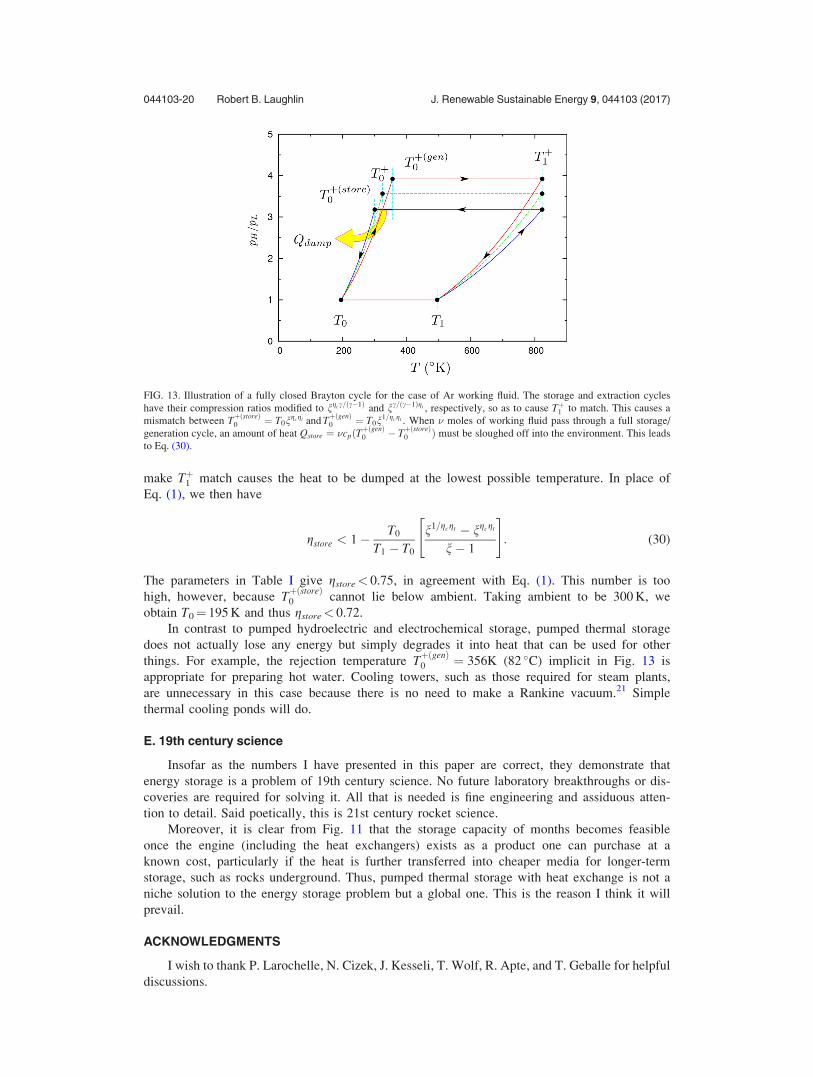
The Brayton cycle requires closing. This is most conveniently accomplished using slightly
different compression ratios for storage and generation, as shown in Fig. 13. Choosing these to
044103-19 Robert B. Laughlin J. Renewable Sustainable Energy 9, 044103 (2017)
make Tþ1 match causes the heat to be dumped at the lowest possible temperature. In place of
Eq. (1), we then have
gstore < 1� T0
T1 � T0
n1=gcgt � ngcgt
n� 1
" #: (30)
The parameters in Table I give gstore< 0.75, in agreement with Eq. (1). This number is too
high, however, because TþðstoreÞ0 cannot lie below ambient. Taking ambient to be 300 K, we
obtain T0¼ 195 K and thus gstore< 0.72.
In contrast to pumped hydroelectric and electrochemical storage, pumped thermal storage
does not actually lose any energy but simply degrades it into heat that can be used for other
things. For example, the rejection temperature TþðgenÞ0 ¼ 356K (82 �C) implicit in Fig. 13 is
appropriate for preparing hot water. Cooling towers, such as those required for steam plants,
are unnecessary in this case because there is no need to make a Rankine vacuum.21 Simple
thermal cooling ponds will do.
E. 19th century science
Insofar as the numbers I have presented in this paper are correct, they demonstrate that
energy storage is a problem of 19th century science. No future laboratory breakthroughs or dis-
coveries are required for solving it. All that is needed is fine engineering and assiduous atten-
tion to detail. Said poetically, this is 21st century rocket science.
Moreover, it is clear from Fig. 11 that the storage capacity of months becomes feasible
once the engine (including the heat exchangers) exists as a product one can purchase at a
known cost, particularly if the heat is further transferred into cheaper media for longer-term
storage, such as rocks underground. Thus, pumped thermal storage with heat exchange is not a
niche solution to the energy storage problem but a global one. This is the reason I think it will
prevail.
ACKNOWLEDGMENTS
I wish to thank P. Larochelle, N. Cizek, J. Kesseli, T. Wolf, R. Apte, and T. Geballe for helpful
discussions.
FIG. 13. Illustration of a fully closed Brayton cycle for the case of Ar working fluid. The storage and extraction cycles
have their compression ratios modified to ngcc=ðc�1Þ and nc=ðc�1Þgt , respectively, so as to cause Tþ1 to match. This causes a
mismatch between TþðstoreÞ0 ¼ T0n
gcgt and TþðgenÞ0 ¼ T0n
1=gcgt . When � moles of working fluid pass through a full storage/
generation cycle, an amount of heat Qstore ¼ �cpðTþðgenÞ0 � T
þðstoreÞ0 Þ must be sloughed off into the environment. This leads
to Eq. (30).
044103-20 Robert B. Laughlin J. Renewable Sustainable Energy 9, 044103 (2017)
1D. Lindley, “The energy storage problem,” Nature 463, 18 (2010).2R. M. Dell and D. A. J. Rand, “Energy storage—a key technology for global energy sustainability,” J. Power Sources100, 2 (2001).
3Z. Luo, J. Wang, M. Dooner, and J. Clarke, “Overview of current development in electrical energy storage technologiesand the application potential in power system operation,” Appl. Energy 137, 511 (2015).
4M. Carbajales-Dale, C. J. Barnhart, and S. M. Benson, “Can we afford storage? A dynamic net energy analysis of renew-able electricity generation supported by energy storage,” Energy Environ. Sci. 7, 1538 (2014).
5D. Weissbach, G. Ruprecht, A. Huke, K. Czerski, S. Gottlieb, and A. Hussein, “Energy intensities, EROIs (EnergyReturn on Invested), and energy payback times of electricity generating power plants,” Energy 52, 210 (2013).
6E. Hittinger and R. Lueken, “Is inexpensive natural gas hindering the grid energy storage industry?,” Energy Policy 87,140 (2015).
7G. Locatelli, E. Palerma, and M. Mancini, “Assessing the economics of large energy storage plants with an optimisationmethodology,” Energy 83, 15 (2015).
8P. Denholm and M. Hand, “Grid flexibility and storage required to achieve very high penetration of variable renewableenergy,” Energy Policy 39, 1817 (2011).
9Renewable Energy Integration, edited by L. E. Jones (Academic Press, New York, 2014).10G. Swindle, Valuation and Risk Management in Energy Markets (Cambridge University Press, Cambridge, 2014).11E. Barbour, G. Wilson, P. Hall, and J. Radcliffe, “Can negative electricity prices encourage inefficient electrical storage
devices?,” Int. J. Environ. Stud. 71, 862 (2014).12D. Droste-Franke, Balancing Renewable Energy (Springer Verlag, Heidelberg, 2012).13J. Howes, “Concept and development of a pumped heat electricity storage device,” Proc. IEEE 100, 493 (2011).14T. Desrues, J. Ruer, P. Marty, and J. F. Fourmogu�e, “A thermal energy storage process for large scale electric
applications,” Appl. Therm. Eng. 30, 425 (2010).15C. P�erilhon, S. Lacour, P. Podevin, and G. Descombes, “Thermal electricity storage by a thermodynamic process: Study
of temperature impact on the machines,” Energy Procedia 36, 923 (2013).16A. Thess, “Thermodynamic efficiency of pumped heat electricity storage,” Phys. Rev. Lett. 111, 110602 (2013).17A. White, G. Parks, and C. N. Markides, “Thermodynamic analysis of pumped thermal electricity storage,” Appl.
Therm. Eng. 53, 291 (2013).18National Academy of Sciences, National Academy of Engineering, and National Research Council, Real Prospects for
Energy Efficiency in the United States (National Academies Press, Washington, DC, 2010), p. 280.19R. L. Garwin and G. Charpak, Megawatts and Megatons (University of Chicago Press, Chicago, 2002).20S. A. Wright, R. F. Radel, M. E. Vernon, G. E. Rochau, and P. S. Pickard, “Operation and analysis of a supercritical
CO2 Brayton cycle,” Sandia National Laboratories, Report No. SAND2010-0171 (2010).21A. S. Leyzerovich, Steam Turbines for Modern Fossil Fuel Power Plants (CRC Press, Boca Raton, FL, 2007).22ASME, 2007 Boiler and Pressure Vessel Code (with Addenda for 2008) (ASME, New York, 2007), Part II, Sec. D,
Subpart 1, Tables 1A and 1B.23H. M€uller-Steinhagen, “Concentrating thermal power,” Philos. Trans. R. Soc. A 371, 20110433 (2013).24R. W. Bradshaw and N. P. Siegel, “Molten nitrate salt development for thermal energy storage in parabolic trough solar
power systems,” Sandia National Laboratory, Report No. ES2008-54174 (2008).25T. Bauer, D. Liang, and R. Tamme, “Recent progress in alkali nitrate/nitrite developments for solar thermal power
applications,” in Molten Salts Chemistry and Technology, edited by M. Gaune-Escard and G. M. Haarberg (Wiley,2014).
26D. J. Rogers and G. J. Janz, “Melting-crystallization and premelting properties of NaNO3–KNO3 enthalpies and heatcapacities,” J. Chem. Eng. Data 27, 424 (1982).
27C. M. Kramer and C. J. Wilson, “The phase diagram of NaNO3–KNO3,” Thermochim. Acta 42, 253 (1980).28X. Zhang, J. Tian, K. Xu, and Y. Gao, “Thermodynamic evaluation of phase equilibria in Na NO3–KNO3 system,”
J. Phase Equilib. 24, 441 (2003).29D. A. Nissen and D. E. Meeker, “Nitrate/nitrite chemistry in NaNO3–KNO3 Melts,” Inorg. Chem. 22, 716 (1983).30E. S. Freeman, “The kinetics of the thermal decomposition of potassium nitrate and of the reaction between potassium
nitrite and oxygen,” J. Phys. Chem. 60, 1487 (1956).31P. Gimenez and S. Fereres, “Effect of heating rates and composition on the thermal decomposition of nitrate based mol-
ten salts,” Energy Procedia 69, 654 (2015).32R. I. Olivares, “The thermal stability of molten nitrite/nitrates salt for solar thermal energy storage in different atmos-
pheres,” Sol. Energy 86, 2576 (2012).33S. H. Goods and R. W. Bradshaw, “Corrosion of stainless steels and carbon steel by molten mixtures of commercial
nitrate salts,” J. Mater. Eng. Perform. 13, 78 (2004).34A. Kruizenga and D. Gill, “Corrosion of iron stainless steels in molten nitrate salt,” Energy Procedia 49, 878 (2014).35G. L. Janz, U. Krebs, H. F. Siegenthaler, and R. P. T. Tomkins, “Molten salts: Volume 3, nitrates, nitrites, and mixtures,”
J. Phys. Chem. Ref. Data 1, 581 (1972).36M. Lasfargues, H. Cao, Q. Geng, and Y. Ding, “Rheological analysis of binary eutectic mixture of sodium and
potassium nitrate and the effect of low concentration CuO nanoparticle addition to its viscosity,” Materials 8, 5194(2015).
37T. Bauer, N. Pfleger, N. Breidenbach, M. Eck, D. Liang, and S. Kaesche, “Material aspects of solar salt for sensible heatstorage,” Appl. Energy 111, 1114 (2013).
38Agency for Toxic Substances and Disease Registry, Toxicological Profile for n-Hexane (U.S. Department of Health andHuman Services, 1999).
39P. Arlien-Søborg, Solvent Neurotoxicity (CRC Press, 1991).40E. J. Conkerton, P. J. Wan, and O. A. Richard, “Hexane and heptane as extraction solvents for cottonseed: A laboratory-
scale study,” J. Am. Oil Chem. Soc. 72, 963 (1995).41H. Dominguez, M. J. Nu~nez, and J. M. Lema, “Enzyme-assisted hexane extraction of soya bean oil,” Food Chem. 54,
223 (1995).
044103-21 Robert B. Laughlin J. Renewable Sustainable Energy 9, 044103 (2017)
42A. Rosenthal, D. L. Pyle, and K. Niranjan, “Aqueous and enzymatic processes for edible oil extraction,” EnzymeMicrob. Technol. 19, 402 (1996).
43T. W. Yergovich, G. W. Swift, and F. Kurata, “Density and viscosity of aqueous solutions of methanol and acetone fromthe freezing point to 10 �C,” J. Chem. Eng. Data 16, 222 (1971).
44F. A. M. M. Goncalves, A. R. Trindade, C. S. M. F. Costa, J. C. S. Bernardo, and I. Johnson, “PVT, viscosity, and sur-face tension of ethanol: New measurements and literature data evaluation,” J. Chem. Thermodyn. 42, 1039 (2010).
45C. W. Kanolt, “Nonflammable liquids for cryostats,” Sci. Pap. Bur. Stand. 20, 619 (1925).46R. Hossaini, M. P. Chipperfield, S. A. Montzka, A. Rap, S. Dhomse, and W. Fang, “Efficiency of short-lived halogens at
influencing climate through depletion of stratospheric ozone,” Nat. Geosci. 8, 186 (2015).47V. P. Brykov, G. K. Mukhamedzyanov, and A. G. Usmanov, “Experimental investigation of the thermal conductivity of
organic fluids at low temperatures,” J. Eng. Phys. 18, 62 (1970) [Inzh.-Fiz. Zh. 18, 82 (1970)].48M. J. Assael, E. Charitidou, C. A. N. de Castro, and W. A. Wakeman, “The thermal conductivity of n-hexane, n-heptane,
and n-decane by the transient hot-wire method,” Int. J. Thermophys. 8, 663 (1987).49E. B. Giller and H. G. Drickamer, “Viscosity of normal paraffins near the freezing point,” Ind. Eng. Chem. 41, 2067
(1949).50B. Knapstad, P. A. Skjølsvik, and H. A. Øye, “Viscosity of pure hydrocarbons,” J. Chem. Eng. Data 34, 37 (1989).51B. Kalinowska, J. Jeli�nska, W. W�oycicki, and J. Stecki, “Heat capacities of liquids at temperatures between 90 and
300 K and at atmospheric pressure I. Method and apparatus, and the heat capacities of n-heptane, n-hexane, and n-prop-anol,” J. Chem. Thermodyn. 12, 891 (1980).
52H. Crauber, “Densitometer for absolute measurements of the temperature dependence of density, partial volumes, andthe thermal expansitivity of solids and liquids,” Rev. Sci. Instrum. 57, 2817 (1986).
53E. W. Lemmon, M. O. McLinden, and D. G. Friend, “Thermophysical properties of fluid systems,” in NIST ChemistryWebbook, NIST Standard Reference Database Number 69, edited by P. J. Linstrom and W. G. Mallard (U.S. NationalInstitute of Standards and Technology, 2013).
54S. K. Roberts and S. A. Sjolander, “Effect of the specific heat ratio on the aerodynamic performance of turbomachinery,”J. Eng. Gas Turbines Power 127, 773 (2005).
55F. P. Incropera and D. P. DeWitt, Fundamentals of Heat and Mass Transfer (Wiley, 2006).56B. J. Mckeon, C. J. Swanson, M. V. Zagarola, R. J. Donnelly, and A. J. Smits, “Friction factors for smooth pipe flow,”
J. Fluid Mech. 511, 41 (2004).57K. Huang, Statistical Mechanics (Wiley, 1963), p. 107.58D. Beck and D. G. Wilson, Gas Turbine Regenerators (Springer, 2011).59L. H. Smith, Jr., “Axial compressor aerodesign evolution at general electric,” J. Turbomach. 124, 321 (2002).60A. R. Wadia, D. P. Wolf, and F. G. Haaser, “Aerodynamic design and testing of an axial flow compressor with pressure
ratio of 23:3:1 for the LM2500þ gas turbine,” J. Turbomach. 124, 331 (2002).61A. F. El-Sayed, Aircraft Propulsion and Gas Turbine Engines (CRC Press, 2008), p. 273.62D. Eckhardt, Gas Turbine Powerhouse, 2nd ed. (Oldenbourg Wissenschaftsverlag, 2014), p. 152.63J. K. Schweitzer and J. D. Smith, “Advanced industrial gas turbine technology readiness demonstration program: Phase
II final report, compressor rig fabrication, assembly and test,” U.S. Department of Energy, Report No. DOE/OR/05035-T2 (1981).
64D. K. Hall, E. M. Greitzer, and C. S. Tan, “Performance limits of axial turbomachine stages,” in Proceedings of theASME Turbo Expo: Part A (ASME, 2012), Vol. 8, p. 479.
65J.-M. Tournier and M. S. El-Genk, “Axial flow, multi-stage turbine and compressor models,” Energy Convers. Manage.51, 16 (2010).
66M. P. Boyce, Gas Turbine Engineering Handbook, 4th ed. (Butterworth-Heinemann, 2011).67L. M. Larosiliere, J. R. Wood, M. D. Hathaway, A. J. Medd, and T. Q. Dang, “Aerodynamic design study of advanced
multistage axial compressor,” National Aeronautics and Space Administration, Report No. NASA/TP-2002-211568(2002).
68ASME, ASME Code for Pressure Piping, B31: An American National Standard (ASME, 2008).69ASTM International, Standard Specification for Seamless Carbon Steel Pipe for High Temperature Service (American
Society for Testing and Materials, ASME, 2006), Paragraph 16-3.70A. Aquaro and M. Pieve, “High temperature heat exchangers for power plants: performance and advanced metallic recu-
perators,” Appl. Therm. Eng. 27, 389 (2007).71N. Tsuzuki, Y. Kato, and T. Ishiduka, “High performance printed circuit heat exchanger,” Appl. Therm. Eng. 27, 1702
(2007).72F. J. Brooks, “GE gas turbine performance characteristics,” GE Power Systems, Report No. GER-3567H (2000).73Black and Veach, Cost and Performance Data for Power Generation Technologies (U.S. National Renewable Energy
Laboratory, 2012).74R. Tidball, J. Bluestein, N. Rodriguez, and S. Knoke, “Cost and performance assumptions for modeling electricity gener-
ation technologies,” U.S. National Renewable Energy Laboratory, Report No. NREL/SR-6A20-48595 (2010).75M. D. Fenton, “Iron and steel,” in 2013 Minerals Yearbook (U.S. Geological Survey, 2015).76L. E. Apodaca, “Nitrogen,” in 2013 Minerals Yearbook (U.S. Geological Survey, 2015).77EIA, Petroleum Marketing Monthly January 2016 (U.S. Energy Information Administration, 2016).78H. P. Loh, J. Lyons, and C. W. White III, “Process equipment cost estimation: Final report,” U.S. National Energy
Technology Laboratory, Report No. DOE/NETL-2002/1169 (2002).79API Standard 650, Welded Steel Tanks for Oil Storage (API Standard, 2012).80B. Christensen, Cost Estimating Guide for Road Construction (U.S. Forest Service, Northern Region Engineering, U.S.
Department of Agriculture, 2011).81Task Committee on Pumped Storage of the Hydropower Committee of the energy Division of the American Society of
Civil Engineers, Compendium of Pumped Storage Plants in the United States (ASCE, 1993).82B. Dunn, H. Kamath, and J.-M. Tarascon, “Electrical energy storage for the grid: A battery of choices,” Science 334,
928 (2011).
044103-22 Robert B. Laughlin J. Renewable Sustainable Energy 9, 044103 (2017)
83D. Rastler, “Electricity energy storage: Technology options,” Electric Power Research Institute, Report No. 1020676(2010).
84J. P. Deane, B. P. O. Gallach�oir, and E. J. McKeogh, “Techno-economic review of existing and new pumped hydroenergy storage plant,” Renewable Sustainable Energy Rev. 14, 1293 (2010).
85S. Rahman, L. M. Al-Hadhrami, and M. M. Alam, “Pumped hydro energy storage system: A technological review,”Renewable Sustainable Energy Rev. 44, 586 (2015).
86T. Reddy, Linden’s Handbook of Batteries, 4th ed. (McGraw-Hill, 2010).87K. E. Aifantis, S. A. Hackney, and R. V. Kumar, High Energy Density Lithium Batteries: Materials, Engineering,
Applications (Wiley-VCH, 2010), p. 72.88R. Van Noorden, “A better battery,” Nature 507, 26 (2014).89E. M. Krieger, J. Cannarella, and C. B. Arnold, “A comparison of lead-acid and lithium-based battery behavior and
capacity fade in off-grid renewable charging applications,” Energy 60, 492 (2013).90G. I. Soloveichik, “Flow batteries: Current status and trends,” Chem. Rev. 115, 11533 (2015).91A. Z. Weber, M. M. Mench, J. P. Meyers, P. N. Ross, J. R. Gostick, and Q. Liu, “Redox flow batteries: A Review,”
J. Appl. Electrochem. 41, 1137 (2011).92K. Gong, X. Ma, K. M. Conforti, K. J. Kuttler, J. B. Grunewald, K. L. Yeager, M. Z. Bazant, S. Gu, and Y. Yan, “A
zinc-iron redox-flow battery under $100 per kWh of system capital cost,” Energy Environ. Sci. 8, 2941 (2015).93H. Kim, D. A. Boysen, J. M. Newhouse, B. L. Spatocco, B. Chung, P. J. Burke, D. J. Bradwell, K. Jiang, A. A.
Tomaszowska, K. Wang, W. Wei, L. A. Ortiz, S. A. Barriga, S. M. Poizeau, and D. R. Sadoway, “Liquid metal batteries:Past, present and future,” Chem. Rev. 113, 2075 (2013).
94D. I. Wood III, J. Li, and C. Daniel, “Prospects for reducing the processing cost of lithium ion batteries,” J. PowerSources 275, 234 (2015).
95G. Pistoia, J.-P. Wiaux, and S. P. Wolsky, Used Battery Collection and Recycling (Elsevier, 2001).96International Review of Experimental Pathology: Transition Metal Toxicity, edited by G. W. Richter and K. Solez
(Academic Press, 1990), Vol. 31.97C. J. Rydh, “Environmental assessment of vanadium redox and lead-acid batteries for stationary energy storage,”
J. Power Sources 80, 21 (1999).98G. Majeau-Bettez, T. R. Hawkins, and A. H. Stromman, “Life cycle environmental assessment of lithium-ion and nickel
metal hydride batteries for plug-in hybrid and battery electric vehicles,” Environ. Sci. Technol. 45, 4548 (2011).99D. A. Notter, M. Grauch, R. Widmer, P. W€ager, A. Stamp, R. Zah, and A.-J. Althaus, “Contribution of Li-ion batteries
to the environmental impact of electric vehicles,” Environ. Sci. Technol. 44, 6550 (2010).100G. Saur and T. Ramsden, “Wind electrolysis: hydrogen cost optimization,” U.S. National Renewable Energy
Laboratory, Report No. NREL/TP-5600-50408 (2011).101P. W. Parfomak, “Energy storage for power grids and electric transportation: A technology assessment,” Congressional
Research Service, CRS Report for Congress. Report No. R42455 (2012).102A. A. Akhil, G. Huff, A. B. Currier, B. C. Kaun, D. M. Rastler, S. B. Chen, A. L. Cotter, D. T. Bradshaw, and W. T.
Gauntlett, “DOE/EPRI electricity storage handbook in collaboration with NRECA,” Sandia National Laboratory, ReportNo. SAND2013-5131 (2015).
103F. S. Barnes and J. G. Levine, Large Energy Storage Systems Handbook (CRC Press, 2011), p. 111.104J. O. Goodson, “History of first U.S. compressed air energy storage (CAES) plant,” Electric Power Research Institute,
Report No. EPRI TR-101751 (1992).105G. Grazzini and A. Milazzo, “A thermodynamic analysis of multistage adiabatic CAES,” Proc. IEEE 100, 461 (2012).106E. Barbour, D. Mignard, Y. Ding, and Y. Li, “Adiabatic compressed air energy storage with packed bed thermal energy
storage,” Appl. Energy 155, 804 (2015).107W. Liu, L. Liu, L. Zhou, J. Huang, U. Zhang, G. Xu, and Y. Yang, “Analysis and optimization of a compressed air
energy storage-combined cycle system,” Entropy 16, 3103 (2014).108B. P. McGrail, C. L. Davidson, D. H. Bacon, M. A. Chamness, S. P. Reidel, F. A. Spane, J. E. Cabe, F. S. Knudsen, M.
D. Bearden, J. A. Horner, H. T. Schaef, and P. D. Thorne, “Techno-economic performance evaluation of compressed airenergy storage in the pacific northwest,” Pacific Northwest National Laboratory, Report No. PNNL-22235 (2013).
109H. Safaei, D. W. Keith, and R. J. Hugo, “Compressed air energy storage (CAES) with compressors distributed at heatloads to enable waste heat utilization,” Appl. Energy 103, 165 (2013).
110CSB, Case Study: Heat Exchanger Rupture and Ammonia Release in Houston, Texas (U.S. Chemical Safety and HazardInvestigation Board, 2011).
111R. X. Faivre Pierret, P. Berne, C. Roussel, and F. Le Guern, “The lake Nyos disaster: Model calculations for the flow ofcarbon dioxide,” J. Vulcanol. Geotherm. Res. 51, 161 (1992).
044103-23 Robert B. Laughlin J. Renewable Sustainable Energy 9, 044103 (2017)