Pyfas Documentation - Read the Docs · •Pipesim (via OpenLink, for all the versions

Pyfas DocumentationRelease 0.2.3

Giuseppe Pagliuca

May 17, 2019

Contents:

1 Introduction to Pyfas 11.1 Wrappers . . . . . . . . . . . . . . . . . . . . . . . . . . . . . . . . . . . . . . . . . . . . . . . . . 11.2 Utilities . . . . . . . . . . . . . . . . . . . . . . . . . . . . . . . . . . . . . . . . . . . . . . . . . . 1

2 Installation 3

3 OLGA tpl files, examples and howto 53.1 Tpl loading . . . . . . . . . . . . . . . . . . . . . . . . . . . . . . . . . . . . . . . . . . . . . . . . 5

4 OLGA ppl files, examples and howto 114.1 Ppl loading . . . . . . . . . . . . . . . . . . . . . . . . . . . . . . . . . . . . . . . . . . . . . . . . 11

5 Unisim usc files 175.1 Usc loading . . . . . . . . . . . . . . . . . . . . . . . . . . . . . . . . . . . . . . . . . . . . . . . . 17

6 Tab files 196.1 Tab file loading . . . . . . . . . . . . . . . . . . . . . . . . . . . . . . . . . . . . . . . . . . . . . . 19

7 GAP interface 23

8 PipeSim interface (via Openlink) 258.1 Run a case . . . . . . . . . . . . . . . . . . . . . . . . . . . . . . . . . . . . . . . . . . . . . . . . 268.2 Node results . . . . . . . . . . . . . . . . . . . . . . . . . . . . . . . . . . . . . . . . . . . . . . . 26

9 SFC interface 27

10 Utilities 29

11 Indices and tables 31

i

ii

CHAPTER 1

Introduction to Pyfas

Pyfas is a python toolbox for flow assurance engineers.

1.1 Wrappers

At this moment in time the toolbox contains wrappers for:

• OLGA

• Unisim Design

• Gap (not yet available)

• Pipesim (via OpenLink, for all the versions <= 2012.4)

• SFC

Olga is the standard de facto for the dynamic simulations of multiphase systems (single pipelines or complex network)in the oil and gas indistry. The simulator has text input and output files; with pyfas you can expose Olga results topython (both trends and profiles) or dump all the results to excel/csv for your post-precessing.

UnisimDesign is mainly a process simulator but can be used also to simulate pipelines or networks in particularproviding some external components. Differently from Olga Unisim (unfortunately) does not use text input or outputfiles, the only way to communicate with the software is via a COM interface using pywin32. Pyfas does not pretendto exposes all the possible functionalities of Unisim, only a very limited subset is available at the moment.

PipeSim is a steady state simulator for both single branches or networks

1.2 Utilities

• Surge volume calculation

• PIRead functionality

1

Pyfas Documentation, Release 0.2.3

Tab files are look-up tables with specific thermodynamic properties at given pressure and temperature intervals usedfor flash calculations by dynamic simulators. These files are generated by thermodynamic simulators (like PTVTsim)and it is good practice to have a look on this information before a dynamic simulation. With pyfas it is possible togenerate 3d plots of all the properties and examine more in detail critical ones.

The surge volume calculation utility returns the surge volume given a drain rate and a liquid flowrate time series. Notmore than a simple discrete integration.

With PIRead it is possible to retrieve PI values from a PI server.

A live demo should be available here below (no installation required)

2 Chapter 1. Introduction to Pyfas

http://mybinder.org:/repo/gpagliuca/pyfas

CHAPTER 2

Installation

pip install pyfas

[ ]:

[1]: import pyfas as faimport pandas as pdimport matplotlib.pyplot as plt

3


4 Chapter 2. Installation

CHAPTER 3

OLGA tpl files, examples and howto

For an tpl file the following methods are available:

• filter_data - return a filtered subset of trends

• extract - extract a single trend variable

• to_excel - dump all the data to an excel file

The usual workflow should be:

1. Load the correct tpl

2. Select the desired variable(s)

3. Extract the results or dump all the variables to an excel file

4. Post-process your data in Excel or in the notebook itself

3.1 Tpl loading

To load a specific tpl file the correct path and filename have to be provided:

[2]: tpl_path = '../../pyfas/test/test_files/'fname = '11_2022_BD.tpl'tpl = fa.Tpl(tpl_path+fname)

3.1.1 Trend selection

A tpl file may contain hundreds of trends, in particular for complex networks. For this reason a filtering method isquite useful. A trend can be specified in an OLGA input files in differnet ways, the identification of a single trendmay be not trivial.

5


The easiest way is to filter all the trends using patters, the command tpl.filter_trends("PT") filters all thepressure trends (or better, all the trends with “PT” in the description, if you have defined a temperature trend in theposition “PTTOPSIDE”, for example, this trend will be selected too). The resulting python dictionaly will have aunique index for each filtered trend that can be used to identify the interesting trend(s). In case of an emply pattern allthe available trends will be reported.

[3]: tpl.filter_data('PT')

[3]: {9: "PT 'POSITION:' 'EXIT' '(PA)' 'Pressure'\n",37: "PT 'POSITION:' 'BOTTOMHOLE' '(PA)' 'Pressure'\n",38: "PT 'POSITION:' 'TUBINGHEAD' '(PA)' 'Pressure'\n",39: "PT 'POSITION:' 'DC6' '(PA)' 'Pressure'\n",40: "PT 'POSITION:' 'DC7' '(PA)' 'Pressure'\n",41: "PT 'POSITION:' 'DC8' '(PA)' 'Pressure'\n",42: "PT 'POSITION:' 'DC9' '(PA)' 'Pressure'\n",43: "PT 'POSITION:' 'RBM' '(PA)' 'Pressure'\n",44: "PT 'POSITION:' 'EXIT' '(PA)' 'Pressure'\n"}

or

[4]: tpl.filter_data("'POSITION:' 'EXIT'")

[4]: {3: "GLT 'POSITION:' 'EXIT' '(KG/S)' 'Total liquid mass flow'\n",4: "GLTHL 'POSITION:' 'EXIT' '(KG/S)' 'Mass flow rate of oil'\n",5: "GLTWT 'POSITION:' 'EXIT' '(KG/S)' 'Mass flow rate of water excluding vapour'\n",6: "GLWVT 'POSITION:' 'EXIT' '(KG/S)' 'Total mass flow rate of water including Vapour→˓'\n",7: "GT 'POSITION:' 'EXIT' '(KG/S)' 'Total mass flow'\n",8: "HOL 'POSITION:' 'EXIT' '(-)' 'Holdup (liquid volume fraction)'\n",9: "PT 'POSITION:' 'EXIT' '(PA)' 'Pressure'\n",10: "QLT 'POSITION:' 'EXIT' '(M3/S)' 'Total liquid volume flow'\n",11: "TM 'POSITION:' 'EXIT' '(C)' 'Fluid temperature'\n",12: "UL 'POSITION:' 'EXIT' '(M/S)' 'Average liquid film velocity'\n",20: "HOL 'POSITION:' 'EXIT' '(-)' 'Holdup (liquid volume fraction)'\n",28: "HOLWT 'POSITION:' 'EXIT' '(-)' 'Water volume fraction'\n",36: "ID 'POSITION:' 'EXIT' '(-)' 'Flow regime: 1=Stratified, 2=Annular, 3=Slug,→˓4=Bubble.'\n",44: "PT 'POSITION:' 'EXIT' '(PA)' 'Pressure'\n",52: "Q2 'POSITION:' 'EXIT' '(W/M2-C)' 'Overall heat transfer coefficient'\n",60: "TM 'POSITION:' 'EXIT' '(C)' 'Fluid temperature'\n",68: "TU 'POSITION:' 'EXIT' '(C)' 'Ambient temperature'\n",76: "TWS 'POSITION:' 'EXIT' '(C)' 'Inner wall surface temperature'\n",84: "QGST 'POSITION:' 'EXIT' '(SM3/S)' 'Gas volume flow at standard conditions'\n",92: "QOST 'POSITION:' 'EXIT' '(SM3/S)' 'Oil volume flow at standard conditions'\n",100: "QWST 'POSITION:' 'EXIT' '(SM3/S)' 'Water volume flow at standard conditions'\n→˓",108: "AL 'POSITION:' 'EXIT' '(-)' 'Void (gas volume fraction)'\n",116: "GG 'POSITION:' 'EXIT' '(KG/S)' 'Gas mass flow'\n",124: "GLT 'POSITION:' 'EXIT' '(KG/S)' 'Total liquid mass flow'\n",132: "GT 'POSITION:' 'EXIT' '(KG/S)' 'Total mass flow'\n",140: "DTHYD 'POSITION:' 'EXIT' '(C)' 'Difference between hydrate and section→˓temperature'\n"}

The same outpout can be reported as a pandas dataframe:

[5]: pd.DataFrame(tpl.filter_data('PT'), index=("Trends",)).T

6 Chapter 3. OLGA tpl files, examples and howto


[5]: Trends9 PT 'POSITION:' 'EXIT' '(PA)' 'Pressure'\n37 PT 'POSITION:' 'BOTTOMHOLE' '(PA)' 'Pressure'\n38 PT 'POSITION:' 'TUBINGHEAD' '(PA)' 'Pressure'\n39 PT 'POSITION:' 'DC6' '(PA)' 'Pressure'\n40 PT 'POSITION:' 'DC7' '(PA)' 'Pressure'\n41 PT 'POSITION:' 'DC8' '(PA)' 'Pressure'\n42 PT 'POSITION:' 'DC9' '(PA)' 'Pressure'\n43 PT 'POSITION:' 'RBM' '(PA)' 'Pressure'\n44 PT 'POSITION:' 'EXIT' '(PA)' 'Pressure'\n

The view_trends method provides the same info better arranged:

[18]: tpl.view_trends('PT')

[18]: Index Variable Position Unit DescriptionFilter: PT0 37 PT POSITION - BOTTOMHOLE PA Pressure1 38 PT POSITION - TUBINGHEAD PA Pressure2 39 PT POSITION - DC6 PA Pressure3 40 PT POSITION - DC7 PA Pressure4 9 PT POSITION - EXIT PA Pressure5 41 PT POSITION - DC8 PA Pressure6 43 PT POSITION - RBM PA Pressure7 44 PT POSITION - EXIT PA Pressure8 42 PT POSITION - DC9 PA Pressure

3.1.2 Dump to excel

To dump all the variables in an excel file use tpl.to_excel() If no path is provided an excel file with the samename of the tpl file is generated in the working folder. Depending on the tpl size this may take a while.

3.1.3 Extract a specific variable

Once you know the variable(s) index you are interested in (see the filtering paragraph above for more info) you canextract it (or them) and use the data directly in python.

Let’s assume you are interested in the inlet pressure and the outlet temperature:

[17]: tpl.view_trends('TM')

[17]: Index Variable Position Unit DescriptionFilter: TM0 59 TM POSITION - RBM C Fluid temperature1 53 TM POSITION - BOTTOMHOLE C Fluid temperature2 54 TM POSITION - TUBINGHEAD C Fluid temperature3 55 TM POSITION - DC6 C Fluid temperature4 56 TM POSITION - DC7 C Fluid temperature5 57 TM POSITION - DC8 C Fluid temperature6 58 TM POSITION - DC9 C Fluid temperature7 11 TM POSITION - EXIT C Fluid temperature8 60 TM POSITION - EXIT C Fluid temperature

3.1. Tpl loading 7


[14]: tpl.view_trends('PT')

[14]: Index Variable Position Unit DescriptionFilter: PT0 37 PT POSITION - BOTTOMHOLE PA Pressure1 38 PT POSITION - TUBINGHEAD PA Pressure2 39 PT POSITION - DC6 PA Pressure3 40 PT POSITION - DC7 PA Pressure4 9 PT POSITION - EXIT PA Pressure5 41 PT POSITION - DC8 PA Pressure6 43 PT POSITION - RBM PA Pressure7 44 PT POSITION - EXIT PA Pressure8 42 PT POSITION - DC9 PA Pressure

Our targets are:

variable 11 - TM ‘POSITION:’ ‘EXIT’ ‘(C)’ ‘Fluid temperature’

and

variable 38 - PT ‘POSITION:’ ‘TUBINGHEAD’ ‘(PA)’ ‘Pressure’

Now we can proceed with the data extraction:

[8]: # single trend extractiontpl.extract(11)tpl.extract(38)

# multiple trends extractiontpl.extract(12, 37)

The tpl object now has the four trends available in the data attribute:

[11]: tpl.data.keys()

[11]: dict_keys([11, 12, 37, 38])

while the label attibute stores the variable type as a dictionary:

[15]: tpl.label

[15]: {11: 'TM POSITION: EXIT (C) Fluid temperature',12: 'UL POSITION: EXIT (M/S) Average liquid film velocity',37: 'PT POSITION: BOTTOMHOLE (PA) Pressure',38: 'PT POSITION: TUBINGHEAD (PA) Pressure'}

3.1.4 Data processing

The results available in the data attribute are numpy arrays and can be easily manipulated and plotted:

[49]: %matplotlib inline

pt_inlet = tpl.data[38]tm_outlet = tpl.data[11]

fig, ax1 = plt.subplots(figsize=(12, 7));ax1.grid(True)p0, = ax1.plot(tpl.time/3600, tm_outlet)

(continues on next page)



(continued from previous page)

ax1.set_ylabel("Outlet T [C]", fontsize=16)ax1.set_xlabel("Time [h]", fontsize=16)

ax2 = ax1.twinx()p1, = ax2.plot(tpl.time/3600, pt_inlet/1e5, 'r')ax2.grid(False)ax2.set_ylabel("Inlet P [bara]", fontsize=16)

ax1.tick_params(axis="both", labelsize=16)ax2.tick_params(axis="both", labelsize=16)

plt.legend((p0, p1), ("Outlet T", "Inlet P"), loc=4, fontsize=16)plt.title("Inlet P and Outlet T for case FC1", size=20);

[4]: import pyfas as faimport pandas as pdimport matplotlib.pyplot as pltpd.options.display.max_colwidth = 120

3.1. Tpl loading 9



CHAPTER 4

OLGA ppl files, examples and howto

For an tpl file the following methods are available:

• filter_data - return a filtered subset of trends

• extract - extract a single trend variable

• to_excel - dump all the data to an excel file

The usual workflow should be:

1. Load the correct tpl

2. Select the desired variable(s)

3. Extract the results or dump all the variables to an excel file

4. Post-process your data in Excel or in the notebook itself

4.1 Ppl loading

To load a specific tpl file the correct path and filename have to be provided:

[5]: ppl_path = '../../pyfas/test/test_files/'fname = 'FC1_rev01.ppl'ppl = fa.Ppl(ppl_path+fname)

4.1.1 Profile selection

As for tpl files, a ppl file may contain hundreds of profiles, in particular for complex networks. For this reason afiltering method is quite useful.The easiest way is to filter on all the profiles using patters, the command ppl.filter_trends("PT") filters allthe pressure profiless (or better, all the profiles with “PT” in the description, if you have defined a temperature profilein the position “PTTOPSIDE”, for example, this profile will be selected too). The resulting python dictionaly will

11


have a unique index for each filtered profile that can be used to identify the interesting profile(s). In case of an emplypattern all the available profiles will be reported.

[6]: ppl.filter_data('PT')

[6]: {4: "PT 'SECTION:' 'BRANCH:' 'old_offshore' '(PA)' 'Pressure'\n",12: "PT 'SECTION:' 'BRANCH:' 'riser' '(PA)' 'Pressure'\n",20: "PT 'SECTION:' 'BRANCH:' 'new_offshore' '(PA)' 'Pressure'\n",28: "PT 'SECTION:' 'BRANCH:' 'to_vent' '(PA)' 'Pressure'\n",36: "PT 'SECTION:' 'BRANCH:' 'dry' '(PA)' 'Pressure'\n",44: "PT 'SECTION:' 'BRANCH:' 'tiein_spool' '(PA)' 'Pressure'\n"}

The same outpout can be reported as a pandas dataframe:

[7]: pd.DataFrame(ppl.filter_data('PT'), index=("Profiles",)).T

[7]: Profiles4 PT 'SECTION:' 'BRANCH:' 'old_offshore' '(PA)' 'Pressure'\n12 PT 'SECTION:' 'BRANCH:' 'riser' '(PA)' 'Pressure'\n20 PT 'SECTION:' 'BRANCH:' 'new_offshore' '(PA)' 'Pressure'\n28 PT 'SECTION:' 'BRANCH:' 'to_vent' '(PA)' 'Pressure'\n36 PT 'SECTION:' 'BRANCH:' 'dry' '(PA)' 'Pressure'\n44 PT 'SECTION:' 'BRANCH:' 'tiein_spool' '(PA)' 'Pressure'\n

4.1.2 Dump to excel

To dump all the variables in an excel file use ppl.to_excel() If no path is provided an excel file with the samename of the tpl file is generated in the working folder. Depending on the tpl size this may take a while.

4.1.3 Extract a specific variable

Once you know the variable(s) index you are interested in (see the filtering paragraph above for more info) you canextract it (or them) and use the data directly in python.

Let’s assume you are interested in the pressure and the temperature profile of the branch riser:

[8]: pd.DataFrame(ppl.filter_data("TM"), index=("Profiles",)).T

[8]: Profiles5 TM 'SECTION:' 'BRANCH:' 'old_offshore' '(C)' 'Fluid temperature'\n13 TM 'SECTION:' 'BRANCH:' 'riser' '(C)' 'Fluid temperature'\n21 TM 'SECTION:' 'BRANCH:' 'new_offshore' '(C)' 'Fluid temperature'\n29 TM 'SECTION:' 'BRANCH:' 'to_vent' '(C)' 'Fluid temperature'\n37 TM 'SECTION:' 'BRANCH:' 'dry' '(C)' 'Fluid temperature'\n45 TM 'SECTION:' 'BRANCH:' 'tiein_spool' '(C)' 'Fluid temperature'\n

[9]: pd.DataFrame(ppl.filter_data("PT"), index=("Profiles",)).T

[9]: Profiles4 PT 'SECTION:' 'BRANCH:' 'old_offshore' '(PA)' 'Pressure'\n12 PT 'SECTION:' 'BRANCH:' 'riser' '(PA)' 'Pressure'\n20 PT 'SECTION:' 'BRANCH:' 'new_offshore' '(PA)' 'Pressure'\n28 PT 'SECTION:' 'BRANCH:' 'to_vent' '(PA)' 'Pressure'\n


12 Chapter 4. OLGA ppl files, examples and howto



36 PT 'SECTION:' 'BRANCH:' 'dry' '(PA)' 'Pressure'\n44 PT 'SECTION:' 'BRANCH:' 'tiein_spool' '(PA)' 'Pressure'\n

Our targets are:

variable 13 for the temperature

and

variable 12 for the pressure

Now we can proceed with the data extraction:

[10]: ppl.extract(13)ppl.extract(12)

The ppl object now has the two profiles available in the data attribute:

[11]: ppl.data.keys()

[11]: dict_keys([12, 13])

while the label attibute stores the variable type:

[12]: ppl.label[13]

[12]: "TM 'SECTION:' 'BRANCH:' 'riser' '(C)' 'Fluid temperature'"

4.1.4 Ppl data structure

The ppl data structure at the moment contains:

• the geometry profile of the branch as ppl.data[variable_index][0]

• the selected profile at the timestep 0 as ppl.data[variable_index][1][0]

• the selected profile at the last timestep as ppl.data[variable_index][1][-1]

In other words the first index is the variable, the second is 0 for the geometry and 1 for the data, the last one identifiesthe timestep.

4.1.5 Data processing

The results available in the data attribute are numpy arrays and can be easily manipulated and plotted:

[13]: %matplotlib inline

geometry = ppl.data[12][0]pt_riser = ppl.data[12][1]tm_riser = ppl.data[13][1]

def ppl_plot(geo, v0, v1, ts):fig, ax0 = plt.subplots(figsize=(12, 7));ax0.grid(True)p0, = ax0.plot(geo, v0[ts])ax0.set_ylabel("[C]", fontsize=16)ax0.set_xlabel("[m]", fontsize=16)


4.1. Ppl loading 13



ax1 = ax0.twinx()p1, = ax1.plot(geo, v1[ts]/1e5, 'r')ax1.grid(False)ax1.set_ylabel("[bara]", fontsize=16)ax1.tick_params(axis="both", labelsize=16)ax1.tick_params(axis="both", labelsize=16)plt.legend((p0, p1), ("Temperature profile", "Pressure profile"), loc=3,

→˓fontsize=16)plt.title("P and T for case FC1", size=20);

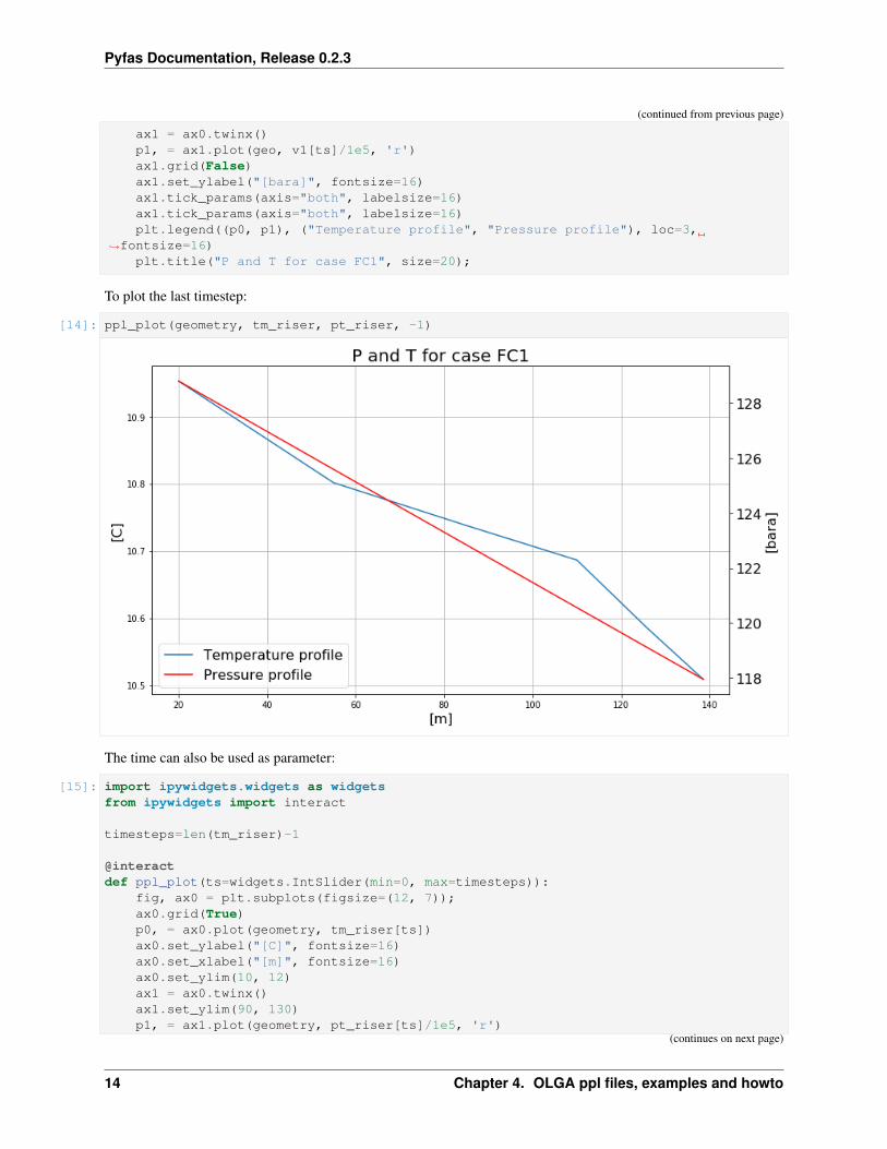
To plot the last timestep:

[14]: ppl_plot(geometry, tm_riser, pt_riser, -1)

The time can also be used as parameter:

[15]: import ipywidgets.widgets as widgetsfrom ipywidgets import interact

timesteps=len(tm_riser)-1

@interactdef ppl_plot(ts=widgets.IntSlider(min=0, max=timesteps)):

fig, ax0 = plt.subplots(figsize=(12, 7));ax0.grid(True)p0, = ax0.plot(geometry, tm_riser[ts])ax0.set_ylabel("[C]", fontsize=16)ax0.set_xlabel("[m]", fontsize=16)ax0.set_ylim(10, 12)ax1 = ax0.twinx()ax1.set_ylim(90, 130)p1, = ax1.plot(geometry, pt_riser[ts]/1e5, 'r')





ax1.grid(False)ax1.set_ylabel("[bara]", fontsize=16)ax1.tick_params(axis="both", labelsize=16)ax1.tick_params(axis="both", labelsize=16)plt.legend((p0, p1), ("Temperature profile", "Pressure profile"), loc=3,

→˓fontsize=16)plt.title("P and T for case FC1 @ timestep {}".format(ts), size=20);

The above plot has an interactive widget if executed

4.1. Ppl loading 15



CHAPTER 5

Unisim usc files

Unisim Design provides some old-fashion API via a COM interface to handle usc files. This interface works only onWindows and more info can be found here (a free registration is required). The Usc class of pyfas exposes in pythona minimal subset of API.

The available methods are:

• extract_profiles

• extract_stripchart

• run_until

• close

• save

Warning: Save and close any Unisim instance before using this class!

5.1 Usc loading

To load a specific usc file the correct path and filename have to be provided:

usc_path = '../../pyfas/test/test_files/'

fname = 'test_case.usc'

usc = fa.Usc(usc_path+fname)

5.1.1 Extract Profiles

Profiles can be extracted with the extract_profiles method: the pipeline name is required

17

http://unisim.supportportal.com/


5.1.2 Extract stripchart

Stripcharts can be extracted with the extract_stripchart method: the defaul stripchart name is overall

5.1.3 Run until

With run_until the simulation is started until the specified endtime (in minures) is reached.

[2]: import pandas as pdimport pyfas as fa

18 Chapter 5. Unisim usc files

CHAPTER 6

Tab files

A tab file contains thermodynamic properties pre-calculated by a thermodynamic simulator like PVTsim. It is goodpractice to analyze these text files before using them. Unfortunately there are several file layouts (key, fixed, withjust a fluid, etc.). The Tab class handles some (most?) of the possible cases but not necessarily all the combinations.The only public method is extract_all and returns a pandas dataframe with the thenrmodynamic properties. Atthis moment in time the dtaframe obtained is not unique, it depends on the tab format and on the number of fluids inthe original tab file. Room to improve here.

6.1 Tab file loading

[14]: tab_path = '../../pyfas/test/test_files/'fname = '3P_single-fluid_key.tab'tab = fa.Tab(tab_path+fname)

6.1.1 Extraction

[15]: tab.export_all()

[16]: tab.data

[16]: "1"CPG [1898.12, 1905.92, 1913.71, 1921.51, 1929.3, 1...CPHL [1610.0, 1617.06, 1623.76, 1630.02, 1635.79, 1...CPWT [3454.74, 3458.93, 3463.33, 3467.94, 3472.76, ...DROGDP [8.4946e-06, 8.42111e-06, 8.34888e-06, 8.27788...DROGDT [-0.000323057, -0.000317492, -0.00031207, -0.0...DROHLDP [4.47091e-07, 4.5376e-07, 4.60533e-07, 4.67363...DROHLDT [-0.694011, -0.693068, -0.691885, -0.69043, -0...DROWTDP [5.24381e-07, 5.22483e-07, 5.1907e-07, 5.14565...DROWTDT [0.158913, 0.142489, 0.120409, 0.0942844, 0.06...


19



HG [-19279.3, -14920.5, -10543.9, -6149.34, -1736...HHL [-317877.0, -313080.0, -308335.0, -303637.0, -...HWT [-1395510.0, -1387580.0, -1379650.0, -1371710....PT [10000.0, 10000.0, 10000.0, 10000.0, 10000.0, ...ROG [0.0849146, 0.0841808, 0.0834595, 0.0827506, 0...ROHL [899.718, 900.424, 901.309, 902.434, 903.838, ...ROWT [813.363, 812.66, 811.929, 811.17, 810.382, 80...RS [0.999977, 0.999979, 0.99998, 0.999982, 0.9999...RSW [0.000692485, 0.000692485, 0.000692484, 0.0006...SEG [1185.33, 1201.82, 1218.24, 1234.58, 1250.85, ...SEHL [-587.526, -570.743, -554.118, -537.594, -521....SEWT [-4115.44, -4085.47, -4055.71, -4026.17, -3996...SIGGHL [0.0280944, 0.0280288, 0.0279906, 0.0279847, 0...SIGGWT [0.0698809, 0.0690383, 0.0682086, 0.0673915, 0...SIGHLWT [0.0551154, 0.0550872, 0.0550879, 0.0551306, 0...TCG [0.0277744, 0.028032, 0.0282904, 0.0285496, 0....TCHL [0.0969043, 0.0960938, 0.0953334, 0.094616, 0....TCWT [0.548681, 0.553425, 0.558072, 0.562624, 0.567...TM [-10.0, -7.70833, -5.41667, -3.125, -0.833333,...VISG [1.01832e-05, 1.02634e-05, 1.03434e-05, 1.0423...VISHL [0.220481, 0.227562, 0.234135, 0.240676, 0.247...VISWT [0.0010661, 0.00101649, 0.000970794, 0.0009286...

Some key info about the tab file are provided as tab.metadata

[17]: tab.metadata

[17]: {'fluids': [' "1"'],'nfluids': 1,'p_array': array([ 1.00000000e+04, 1.01325000e+05, 7.38958000e+05,

1.46792000e+06, 2.19688000e+06, 2.92583000e+06,3.65479000e+06, 4.38375000e+06, 5.11271000e+06,5.84167000e+06, 6.57063000e+06, 7.29958000e+06,8.02854000e+06, 8.75750000e+06, 9.48646000e+06,1.02154000e+07, 1.09444000e+07, 1.16733000e+07,1.24023000e+07, 1.31313000e+07, 1.38602000e+07,1.45892000e+07, 1.53181000e+07, 1.60471000e+07,1.67760000e+07, 1.75050000e+07, 1.82340000e+07,1.89629000e+07, 1.96919000e+07, 2.04208000e+07,2.11498000e+07, 2.18788000e+07, 2.26077000e+07,2.33367000e+07, 2.40656000e+07, 2.47946000e+07,2.55235000e+07, 2.62525000e+07, 2.69815000e+07,2.77104000e+07, 2.84394000e+07, 2.91683000e+07,2.98973000e+07, 3.06263000e+07, 3.13552000e+07,3.20842000e+07, 3.28131000e+07, 3.35421000e+07,3.42710000e+07, 3.50000000e+07]),

'p_points': 50,'properties': ['PT','TM','ROG','ROHL','ROWT','DROGDP','DROHLDP','DROWTDP','DROGDT','DROHLDT',


20 Chapter 6. Tab files



'DROWTDT','RS','RSW','VISG','VISHL','VISWT','CPG','CPHL','CPWT','HG','HHL','HWT','TCG','TCHL','TCWT','SIGGHL','SIGGWT','SIGHLWT','SEG','SEHL','SEWT'],

't_array': array([ -10. , -7.70833 , -5.41667 , -3.125 , -0.833333,1.45833 , 3.75 , 6.04167 , 8.33333 , 10.625 ,

12.9167 , 15.2083 , 15.56 , 17.5 , 19.7917 ,22.0833 , 24.375 , 26.6667 , 28.9583 , 31.25 ,33.5417 , 35.8333 , 38.125 , 40.4167 , 42.7083 ,45. , 47.2917 , 49.5833 , 51.875 , 54.1667 ,56.4583 , 58.75 , 61.0417 , 63.3333 , 65.625 ,67.9167 , 70.2083 , 72.5 , 74.7917 , 77.0833 ,79.375 , 81.6667 , 83.9583 , 86.25 , 88.5417 ,90.8333 , 93.125 , 95.4167 , 97.7083 , 100. ]),

't_points': 50}

6.1.2 Plotting

Here under an example of a 3D plot of the liquid hydropcarbon viscosity

[48]: import matplotlib.pyplot as pltfrom mpl_toolkits.mplot3d import Axes3Dimport itertools as it

def plot_property_keyword(pressure, temperature, thermo_property):fig = plt.figure(figsize=(16, 12))ax = fig.add_subplot(111, projection='3d')X = []Y = []for x, y in it.product(pressure, temperature):

X.append(x/1e5)Y.append(y)

ax.scatter(X, Y, thermo_property)ax.set_ylabel('Temperature [C]')ax.set_xlabel('Pressure [bar]')ax.set_xlim(0, )ax.set_title('ROHL')return fig

6.1. Tab file loading 21


[49]: plot_property_keyword(tab.metadata['p_array'],tab.metadata['t_array'],tab.data.T['ROHL'].values[0])

[49]:

[ ]:

22 Chapter 6. Tab files

CHAPTER 7

GAP interface

GAP provides a comfortable set of API via the OpenServer interface. This interface works, of course, only on Windowsand provides a CLI access to most of the simulator features. Pyfas is not required to use OpenServer.

This example uses pywin32, but any package providing a COM interface should work:

# Connecting to the open GAP file

from win32com.client import Dispatch

gap = Dispatch('PX32.OpenServer.1')

The previous command gives the possibility to interact with an open GAP model (open via the UI). In case more thanone model is open, the last one opened is considered.It is also possible to access to closed models:

gap.docommand('GAP.START')

gap.docommand(r'GAP.OpenFile("C:\example\example.gap")')

Two basic operations are possible:

• getvalue

• setvalue

Pretty straightforward, isn’t it?

# This command shows the flow correlation for the Pipe1 of the model {PROD}

gap.getvalue("GAP.MOD[{PROD}].PIPE[1].PIPECORR")

Out[4]: 'MukerjeeBrill'

23


To set a value instead:

# This command sets the flowrate of SOURCE1 to 10 (it uses predefined unit)

gap.setvalue("GAP.MOD[{PROD}].SOURCE[{Source1}].Rate", 10)

It looks complicated but a good reference guide is available and, even better, with the right click in the GUI thecorresponding OpenServer command can be showed in the OpenServer window:

24 Chapter 7. GAP interface

CHAPTER 8

PipeSim interface (via Openlink)

The OpenLink functionality (available for all the PipeSim versions <= 2012.4) provides a COM interface to both singlebranch and network models.

Like for other COM interfaces the Dispatch method of the pywin32 module can be used to communicate withPipeSim. For example to open the a network model called base_model.bpn you can:

o = Dispatch("NET32COM.INetModel")

o.OpenModel(path_to/base_model.bpn)

Once loaded the model all the the different elements can be checked or modified: o.GetNameList(i) returns a2-elements tuple containing the all the names and the number of elements corresponding to the index i. For example:

o.GetNameList(2)[0]

would return all the names of the sources of the model.

Once the name of the source you want to modify is known it is possilbe to use o.SetBoundaryFluidrate todefine a new fluid rate:

o.SetBoundaryFluidrate(source_name, 0, new_value, 'STB/d')

SetBoundaryFluidrate as second parameter accepts an integer:

• 0 for liquid flowrate

• 1 for gas flowrate

o.SaveModel

can be use to save as (it requires as parameter the path and the new name of the model as a string)

25


8.1 Run a case

To run a case in the background:

o.RunNetwork2(False, "-B")

and to check if it is still simulating:

o.GetIsModelRunning()

8.2 Node results

Node results can be estracted using the Dispatch("PNSREADER.PNSCom"):

results.ReadPnsFile(pns_file_path)

idx = results.GetNodeIndex(interesting_node)

pt = results.GetNodeVariableValue(idx, 'Pressure')

26 Chapter 8. PipeSim interface (via Openlink)

CHAPTER 9

SFC interface

Prvinding you have available the SFC dlls this wrapper allows you to run SFC directly from python.

Here an example (Win platform only):

import pyfas as fasfc = fa.SFC()case = sfc.default_input()df = sfc.run(**case)dp_fr = df[“Frictional pressure gradient (> 0 for dp_f/dx < 0) [N/m3]”]hol = df[“Liquid volume fraction [fraction]”]

A pandas dataframe with all the input and potential output is returned.

[33]: import pyfas as faimport pandas as pdimport matplotlib.pyplot as plt

27


28 Chapter 9. SFC interface

CHAPTER 10

Utilities

29


30 Chapter 10. Utilities

CHAPTER 11

Indices and tables

• genindex

• modindex

• search

31

Date post:	22-Mar-2020
Category:	Documents
Upload:	others
View:	39 times
Download:	0 times

Pyfas Documentation - Read the Docs · •Pipesim (via OpenLink, for all the versions

Documents