ABSTRACTKernel density visualization, or KDV, is used to view andunderstand data points in various domains, including trafficor crime hotspot detection, ecological modeling, chemicalgeology, and physical modeling. Existing solutions, whichare based on computing kernel density (KDE) functions, arecomputationally expensive. Our goal is to improve the perfor-mance of KDV, in order to support large datasets (e.g., one mil-lion points) and high screen resolutions (e.g., 1280 × 960 pix-els). We examine two widely-used variants of KDV, namelyapproximate kernel density visualization (ϵKDV) and thresh-olded kernel density visualization (τKDV). For these twooperations, we develop fast solution, called QUAD, by deriv-ing quadratic bounds of KDE functions for different typesof kernel functions, including Gaussian, triangular etc. Wefurther adopt a progressive visualization framework for KDV,in order to stream partial visualization results to users con-tinuously. Extensive experiment results show that our newKDV techniques can provide at least one-order-of-magnitudespeedup over existing methods, without degrading visual-ization quality. We further show that QUAD can producethe reasonable visualization results in real-time (0.5 sec) bycombining the progressive visualization framework in singlemachine setting without using GPU and parallel computation.ACM Reference Format:Tsz Nam Chan, Reynold Cheng and Man Lung Yiu. 2019. QUAD:Quadratic-Bound-based Kernel Density Visualization. In Proceed-ings of ACM (SIGMOD). ACM, New York, NY, USA, 18 pages.https://doi.org/10.1145/nnnnnnn.nnnnnnn1 INTRODUCTIONData visualization [8, 24, 25] is an important tool for un-derstanding a dataset. In this paper, we study kernel-density-estimation-based visualization [43] (termed kernel density
visualization (KDV) here), which is one of the most com-monly used data visualization solutions. KDV is often usedin hotspot detection (e.g., in criminology and transporta-tion) [4, 20, 45, 49, 51] and data modeling (e.g., in ecology,chemistry, and physics) [3, 10, 29, 30, 46]. Most of these ap-plications restrict the dimensionality of datasets to be smallerthan 3 [4, 20, 29, 30, 45, 46, 49, 51].1 Figure 1 shows theuse of KDV in analyzing motor vehicle thefts in Arlington,Texas in 2007. Here, each black dot is a data point, whichdenotes the place where a crime has been committed. A colormap, which represents the criminal risk in different places,is generated by KDV; for instance, a red region indicatesthe highest risk of vehicle thefts in that area. As discussedin [4, 20], color maps are often used by social scientists orcriminologists for data analysis.
Table 1 summarizes the usage of KDV in different domains.Due to its wide applicability, KDV is often provided in dataanalytics platforms, including Scikit-learn 2, ArcGIS 3, andQGIS 4.
Table 1: KDV ApplicationsType domain Usage Ref.
Hotspot Criminology Detection of crime regions [4, 20, 53]detection Transportation Detection of traffic hotspots [45, 49, 51]
Data Ecology Visualization of polluted [21, 29, 30]modeling regions
Chemistry Visualization of detrial [46]age distributions
Physics Particle searching [3, 10]
To generate a color map (e.g., Figure 1), KDV determinesthe color value of each pixel q on the two-dimensional com-puter screen by a kernel density (KDE) function, denoted byFP (q) [43]. Equation 1 shows one example of FP (q) withGaussian kernel, where P and dist(q, pi) are the set of two-dimensional data points and Euclidean distance respectively.
FP (q) =∑pi∈P
w · exp(−γdist(q, pi)2) (1)
1For high-dimensional dataset, one approach is to first use dimension reduc-tion techniques (e.g., [48]) to reduce the dimension to 1 or 2 and then utilizeKDV to generate color map.2https://scikit-learn.org/3http://pro.arcgis.com/en/pro-app/tool-reference/spatial-analyst/how-kernel-density-works.htm4https://docs.qgis.org/2.18/en/docs/user_manual/plugins/plugins_heatmap.html
SIGMOD, 2020 Tsz Nam Chan, Reynold Cheng and Man Lung Yiu
Figure 1: A color map for motor vehicle thefts (blackdots) in Arlington, Texas in 2007 (Cropped from [20])
In this paper, we will also consider FP (q) with other kernelfunctions in Section 5. As a remark, all kernel functions, thatwe consider in this paper, are adopted in famous software,e.g., Scikit-learn [35] and QGIS [40].
A higher FP (q) value indicates a higher density of datapoints in the region around q. The above KDE function is com-putationally expensive to compute. Given a data set with 1 mil-lion 2D points, KDV involves over 2 trillion operations [36]on a 1920×1080 screen. As pointed out in [13, 16, 52, 55, 56],KDV cannot scale well to handle many data points and dis-play of color maps on high-resolution screens. To addressthis problem, researchers have proposed two variants of KDV,which aim to improve its performance:• ϵKDV: This is an approximate version of KDV. A relativeerror parameter, ϵ , is used, such that for each pixel q, thepixel color is within (1± ϵ) of FP (q). Figure 2a shows a colormap generated by the original (exact) KDV, while Figure2b illustrates the corresponding color map for ϵKDV withϵ equal to 0.01. As we can see, the two color maps do notlook different. ϵKDV runs faster than exact KDV [7, 17, 54–56], and is also supported in data analytics software (e.g.,Scikit-learn [35]).• τKDV: In tasks such as hotspot detection [4, 20], a datavisualization user only needs to know which spatial regionhas a high density (i.e., hotspot), and not the other areas. Onesuch hotspot is the red region in Figure 1. A color map withtwo colors are already sufficient. Figure 2c shows such acolor map. To generate this color map, the τKDV can be used,where a threshold, τ , detemines the color of a pixel: a colorfor q when FP (q) ≥ τ (to indicate high density), and anothercolor otherwise. This method, recently studied in [7, 13], isshown to be faster than exact KDV.
Although ϵKDV and τKDV perform better than exact KDV,they still require a lot of time. On a 270k-point crime dataset[1], displaying a color map on a screen with 1280× 960 pixelstakes over an hour for most methods, including the ϵKDV so-lution implemented in Scikit-learn. In fact, these existing
methods often cannot deliver real-time performance, whichallows color maps to be generated quickly, thereby saving theprecious waiting time of data analysts.
Our contributions. In this paper, we develop a solution,called QUAD, in order to improve the performance of ϵKDVand τKDV. The main idea is to derive lower and upper boundsof the KDE function (i.e., Equation 1) in terms of quadraticfunctions (cf. Section 4). These quadratic bounds are theo-retically tighter than the existing ones (in aKDE [17], tKDC[13], and KARL [7]), enabling faster pruning. In addition,many KDV-based applications [11, 15, 20, 27] also utilizeother kernel functions, including triangular, cosine kernelsetc. Therefore, we extend our techniques to support otherkernel functions (cf. Section 5), which cannot be supportedby the state-of-the-art solution, KARL [7]. In our experimentson large datasets in a single machine, QUAD is at least one-order-of-magnitude faster than existing solutions. For ϵKDV,QUAD takes 100-1000 sec to generate color map for eachlarge-scale dataset (0.17M to 7M) with 2560 × 1920 pixels,using small relative error ϵ = 0.01. However, most of theother methods fail to generate the color map within 2 hoursunder the same setting. For τKDV, QUAD can achieve nearly10 sec with 1280 × 960 pixels, using different thresholds.
We further adopt a progressive visualization framework forKDV (cf. Section 6), in order to continuously output partialvisualization results (by increasing the resolution). A user canterminate the process anytime, once the partial visualizationresults are satisfactory, instead of waiting for the precise colormap to be generated. Experiment results show that we canachieve real-time (0.5 sec) in single machine without usingGPU and parallel computation by combining this frameworkwith our solution QUAD.
The rest of the paper is organized as follows. We first reviewexisting work in Section 2. We then discuss the backgroundin Section 3. Later, we present quadratic bound functions forKDE in Section 4. After that, we extend our quadratic boundsto other kernel functions in Section 5. We then discuss ourprogressive visualization framework for KDV in Section 6.Lastly, we show our results in Section 7, and conclude inSection 8. The appendix is shown in Section 9.2 RELATED WORKKernel density visualization (KDV) is widely used in manyapplication domains, such as: ecological modeling [29, 30],crime [4, 20, 53] or traffic hotspot detection [45, 49, 51],chemical geology [46] and physical modeling [10]. For eachapplication, they either need to compute the approximatekernel density values with theoretical guarantee [17] (ϵKDV)or test whether density values are above a given threshold [13](τKDV) in the spatial region. Due to the high computationalcomplexity, many existing algorithms have been developedfor efficient computation of these two variants of KDV, whichcan be divided into three camps (cf. Table 2).
QUAD: Quadratic-Bound-based Kernel Density Visualization SIGMOD, 2020
(a) Exact KDV (b) εKDV, ε=0.01 (c) KDV
Figure 2: Illustrating ϵKDV and τKDVTable 2: Existing methods in KDV
In the first camp, researchers propose function approxima-tion methods for KDE function (cf. Equation 1). Raykar etal. [41] and Yang et al. [50] propose using fast Gauss trans-form to efficiently and approximately compute KDE function.However, this type of methods normally does not provide thetheoretical guarantee between the returned value and exactresult.
In the second camp, researchers propose efficient algorithmby sampling the original datasets. Zheng et al. [54–56] andPhillips et al. [37–39] pre-sample the datasets into smallersizes and apply exact KDV for the reduced datasets. Theyproved that the output result is near the exact KDE value foreach pixel in original datasets. However, their work [37, 54–56] only aim to provide the probabilistic error guarantee (e.g.,ϵ = 0.01 with probability 0.8). On the other hand, determin-istic guarantee (e.g., ϵ = 0.01), used in our problem settings[7, 13, 17], are adopted in existing software, e.g., Scikit-learn[35]. Moreover, their algorithms still need to evaluate theexact KDV for the reduced datasets, which can still be time-consuming. Some other research studies [33, 34] also adoptthe sampling methods for different tasks (e.g., visualizationand query processing). Park et al. [33] propose advancedmethod for sampling the datasets in the preprocessing stage,which is possible to further reduce the sample size, and gen-erate the visualization in the online stage. However, the largepreprocessing time is not acceptable in our setting, since thevisualized datasets are not known in advance for the scientificapplications (cf. Table 1) and software (e.g., Scikit-learn, Ar-cGIS and QGIS). In addition, unlike the sampling methods forKDV (e.g., [54]), since these methods [33, 34] do not discusshow to appropriately update the weight value for each datapoint in the output sample set for the new kernel aggregationfunction 5, they cannot support KDV.
In the third camp, which we are interested in, researcherspropose different efficient lower and upper bound functions5We replace P andw by output sample set andwi in Equation 1 respectively.
with index structure (e.g., kd-tree) to evaluate KDE functions(e.g., Equation 1). Albeit there are many existing work fordeveloping new bound functions [7, 13, 17], there is one keydifference between our proposal QUAD and these methods.Our proposed quadratic bound functions are tighter than all ex-isting bound functions in previous literatures [7, 13, 17] withonly a slight overhead (O(d2) time complexity) for Gaussiankernel, which is affordable as the dimensionality d is normallysmall (d < 3) in KDV, and only in O(d) time complexity forother kernel functions (e.g., triangular and cosine kernels).On the other hand, some other research studies in approxi-mation theory [9, 47] also focus on utilizing the polynomialfunctions to approximate the more complicated functions,e.g., interpolation and curve-fitting. However, these methodscannot provide the correctness guarantee of lower and upperbounds for kernel aggregation function (cf. Equation 1). Inaddition, high-order polynomial functions cannot provide fastevaluation in our setting (e.g., O(d2) time complexity).
Interactive visualization is a well-studied problem [12, 14,24–26, 36, 48, 57]. Users can control the visualization qualityunder different resolutions (e.g., 256 × 256 or 512 × 512) [36].However, existing work either utilize modern hardware (e.g.,GPU) [26, 36]/distributed algorithms (e.g., MapReduce) [36]to support KDV in real-time or do not focus on KDV [12,14, 24, 25, 48, 57]. In this work, we adopt a progressivevisualization framework for KDV which aims to continuouslyprovide coarse-to-fine partial visualization results to users.Users can stop the process at any time once they are satisfiedwith the visualization results. By using our solution QUADand this framework, we can achieve satisfactory visualizationquality (nearly no degradation) in real-time (0.5 sec) in singlemachine setting without using GPU and parallel computation.
There are also many other studies for utilizing paral-lel/distributed computation, e.g., MapReduce [54], and mod-ern hardware, e.g., GPU [52] and FPGA [16], to further boostthe efficiency evaluation of exact KDV. In this work, we focuson single machine setting with CPU and leave the combina-tion of our method QUAD with these optimization opportuni-ties in our future work.
In both database and visualization communities, there arealso many recent visualization tools, which are not basedon KDV [18, 19, 23, 28, 31, 32, 42, 48]. This type of workmainly focuses on avoiding the overplotting effect (i.e., too
SIGMOD, 2020 Tsz Nam Chan, Reynold Cheng and Man Lung Yiu
many points in the spatial region) of the visualization of datapoints in maps or scatter plots. Some other visualization toolsare also summarized in the book [44]. However, in someapplications, e.g., hotspot detection and data modeling (cf.Table 1), the users mainly utilize KDV for visualizing thedensity of different regions in which these work cannot beapplied in this scenario.
3 PRELIMINARIESIn this section, we first revisit the concepts [7, 13, 17] ofbound functions (cf. Section 3.1) and the indexing framework(cf. Section 3.2). Then, we also illustrate the state-of-the-artbound functions [7] (cf. Section 3.3), which are mostly relatedto our work.
3.1 Bound FunctionsIn existing literatures [7, 13, 17], they develop the lowerbound LB(q) and upper bound UB(q) for FP (q) (cf. Equa-tion 1), given the pixel q, which must fulfill the followingcorrectness condition:
LB(q) ≤ FP (q) ≤ UB(q)
For ϵKDV and τKDV, we can avoid evaluating the compu-tationally expensive operation FP (q) ifUB(q) ≤ (1 + ϵ)LB(q)for ϵKDV and LB(q) ≥ τ or UB(q) ≤ τ for τKDV [7]. There-fore, once the bound functions are (1) tighter (near the exactFP (q)) and (2) fast to evaluate (much faster than FP (q)), wecan achieve significant speedup compared with the exact eval-uation of FP (q).
3.2 Indexing Framework for BoundFunctions
Existing literatures [7, 13, 17] adopt the hierarchical indexstructures (e.g., kd-tree) to index the point set P (cf. Figure3).6 We illustrate the running steps (cf. Table 3) for evaluatingthe ϵKDV and τKDV in this indexing framework. In thefollowing, we denote the exact value, lower and upper boundsbetween the pixel q and node Ri to be FRi (q), LBRi (q) andUBRi (q) respectively, where: LBRi (q) ≤ FRi (q) ≤ UBRi (q).
R5
p1 p2 … p5
Rroot
p6 p7 … p9
leaf R1
p10 p11 … p13 p14 p15 … p18
leaf R3leaf R2 leaf R4
R6
Figure 3: Hierarchical index structure for differentbound functions [7, 13, 17]
6The data analytics software, Scikit-learn [35], utilizes kd-tree by default forsolving ϵKDV.
Initially, the algorithm evaluates the bound functions of rootnode Rroot and then pushes back this node into the priorityqueue. This priority queue manages the evaluation order ofdifferent nodes Ri based on the decreasing order of bounddifferenceUBRi (q) −LBRi (q). In each iteration, the algorithmpops out the node with the highest priority, pushes back itschild nodes and maintain the incremental bound values lb andub (e.g., Rroot is popped, its child nodes R5 and R6 are addedand the bounds lb and ub are updated in step 2). Once thepopped node is the leaf (e.g., R1 in step 4), the exact value forthat node is evaluated.Table 3: Running steps for each q in the indexing frame-work
Step Priority Maintenance of lower bound lb Poppedqueue and upper bound ub node
The algorithm terminates for each pixel q in (1) ϵKDVand (2) τKDV once the incremental bounds satisfy (1) ub ≤
(1+ϵ)lb and (2) lb ≥ τ or ub ≤ τ respectively (cf. Section 3.1).Since we follow the same indexing framework as [7, 13, 17],we omit the detailed algorithm here. Interested readers canrefer to the algorithm from the supplementary notes7 of [7].Similar technique can be also found in similarity search com-munity [5, 6]. Even though the worst case time complexityof this algorithm for a given pixel q is O(nB logn + nd) time(B is the evaluation time of each LBRi (q)/UBRi (q)), whichis even higher than directly evaluating FP (q) (O(nd) time),this algorithm is very efficient if we utilize the fast and tightbound functions.3.3 State-of-the-art Bound FunctionsAmong most of the existing bound functions, Chan et al. [7]developed the most efficient and tightest bound functionsfor Equation 1. They utilize the linear function Linm,k (x) =mx + k to approximate the exponential function exp(−x). Wedenote EL(x) = mlx + kl and EU (x) = mux + ku for thelower and upper bounds of exp(−x) respectively, i.e., EL(x) ≤exp(−x) ≤ EU (x), as shown in Figure 4.
Once they set x = γdist(q, pi)2, they can obtain the lin-ear lower and upper bound functions FLP (q, Linm,k ) =∑
pi∈P w(mγdist(q, pi)2 + k) for FP (q) =∑
pi∈P w exp(−γ ·
dist(q, pi)2), given the suitable choices of m and k. They
QUAD: Quadratic-Bound-based Kernel Density Visualization SIGMOD, 2020
0
0.2
0.4
0.6
0.8
1
0.0 0.5 1.0 1.5 2.0
x axis
function value
function
exp(–x)𝐸𝐿(𝑥)= ml x + kl
xmin
x1
x2
x3 xmax
0
0.2
0.4
0.6
0.8
1
0.0 0.5 1.0 1.5 2.0
x axis
function value
function
exp(–x)
xmin
x1
x2
x3
xmax
𝐸𝑈(𝑥) = mu x + ku
(a) Linear lower bound (b) Linear upper bound
Figure 4: Linear lower and upper bound functions for exponential function exp(−x) (from [7])
prove that these bounds are tighter than existing bound func-tions [13, 17]. In addition, they also prove that their linearbounds FLP (q, Linm,k ) can be computed in O(d) time [7](cf. Lemma 1). More details can be found from [7]7.
LEMMA 1. [7] Given two values m and k,FLP (q, Linm,k ) =
∑pi∈P w(mγdist(q, pi)2 + k) can be
computed in O(d) time.
The main idea of achieving these efficient bounds is basedon the fast evaluation of the sum of squared distance, whichcan be achieved in O(d) time [7], given the precomputedaP =
∑pi∈P pi, bP =
∑pi∈P | |pi | |2 and |P |.∑
pi∈P
dist(q, pi)2 =∑pi∈P
(| |q| |2 − 2q · pi + | |pi | |2)
= |P | · | |q| |2 − 2q · aP + bP
4 QUADRATIC BOUNDSAs illustrated in Section 3, if we can develop the fast andtighter bound functions for FP (q), we can achieve significantspeedup for solving both ϵKDV and τKDV. Therefore, we aska question, can we develop the new bound functions, whichare fast and tighter, compared with the state-of-the-art linearbounds [7] (i.e., FLP (q, Linm,k ))? To answer this question,we utilize the quadratic function Q(x) = ax2 +bx +c, (a > 0),to approximate the exponential function exp(−x). Observefrom Figure 5, quadratic function can achieve the lower andupper bounds (QL(x) and QU (x) respectively) of exp(−x)with the suitable choice of the parameters a, b and c, given[xmin, xmax ] as the bounding interval of xi = γdist(q, pi)2
(white circle), i.e., xmin ≤ xi ≤ xmax , where xmin and xmaxare based on the minimum and maximum distances between qand the bounding rectangle of pi respectively [7] (O(d) time).In this paper, we let QL(x) and QU (x) be:
QL(x) = aℓx2 + bℓx + cℓ
QU (x) = aux2 + bux + cu
0
0.2
0.4
0.6
0.8
1
0 1 2 3 4xmin xmaxx1 x2 x3
𝑄𝐿 𝑥 = 0.2𝑥2 − 0.82𝑥 + 0.97
𝑄𝑈 𝑥 = 0.1𝑥2 − 0.56𝑥 + 0.86
function value
function: exp(−𝑥)
Figure 5: Quadratic lower (red) and upper (purple)bound functions of exp(−x) in the range [xmin, xmax ]
We define the aggregation of the quadratic function as:
FQP (q,Q) =∑pi∈P
w(a(γdist(q, pi)2)2 + bγdist(q, p)2 + c
)(2)
With the above concept, FQP (q,QL) and FQP (q,QU ) canserve as the lower and upper bounds respectively for FP (q),as stated in Lemma 2. We include the formal proof of Lemma2 in Section 9.1.
LEMMA 2. If QL(x) and QU (x) are the lower and upperbounds for exp(−x) respectively, we have FQP (q,QL) ≤
FP (q) ≤ FQP (q,QU ).
4.1 Fast Evaluation of Quadratic BoundsIn the following lemma, we illustrate how to efficiently com-pute the bound function FQP (q,Q) inO(d2) time in the querystage (cf. Lemma 3). We leave the proof in Section 9.2.
LEMMA 3. Given the coefficients a, b and c of quadraticfunction Q , FQP (q,Q) can be computed in O(d2) time.
Although the computation time of FQP (q,Q) is slightlyworse than [7], which is only in O(d) time, this overhead isnegligible as the dimensionality of datasets is smaller than 3
SIGMOD, 2020 Tsz Nam Chan, Reynold Cheng and Man Lung Yiu
in KDV. However, as we will show in the following sections,our bounds are tighter than the existing bound functions [7].
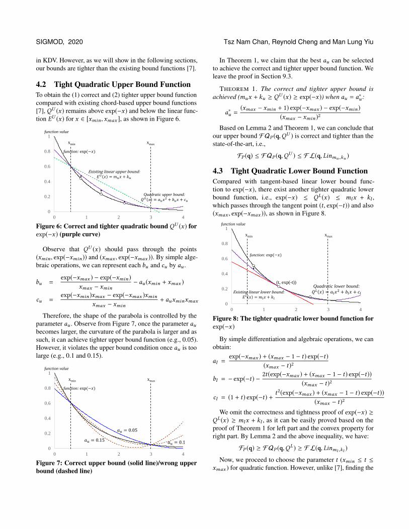
4.2 Tight Quadratic Upper Bound FunctionTo obtain the (1) correct and (2) tighter upper bound functioncompared with existing chord-based upper bound functions[7], QU (x) remains above exp(−x) and below the linear func-tion EU (x) for x ∈ [xmin, xmax ], as shown in Figure 6.
Observe that QU (x) should pass through the points(xmin, exp(−xmin)) and (xmax , exp(−xmax )). By simple alge-braic operations, we can represent each bu and cu by au .
bu =exp(−xmax ) − exp(−xmin)
xmax − xmin− au (xmin + xmax )
cu =exp(−xmin)xmax − exp(−xmax )xmin
xmax − xmin+ auxminxmax
Therefore, the shape of the parabola is controlled by theparameter au . Observe from Figure 7, once the parameter aubecomes larger, the curvature of the parabola is larger and assuch, it can achieve tighter upper bound function (e.g., 0.05).However, it violates the upper bound condition once au is toolarge (e.g., 0.1 and 0.15).
In Theorem 1, we claim that the best au can be selectedto achieve the correct and tighter upper bound function. Weleave the proof in Section 9.3.
THEOREM 1. The correct and tighter upper bound isachieved (mux + ku ≥ QU (x) ≥ exp(−x)) when au = a∗u :
a∗u =(xmax − xmin + 1) exp(−xmax ) − exp(−xmin)
(xmax − xmin)2
Based on Lemma 2 and Theorem 1, we can conclude thatour upper bound FQP (q,QU ) is correct and tighter than thestate-of-the-art, i.e.,
FP (q) ≤ FQP (q,QU ) ≤ FL(q, Linmu ,ku )
4.3 Tight Quadratic Lower Bound FunctionCompared with tangent-based linear lower bound func-tion to exp(−x), there exist another tighter quadratic lowerbound function, i.e., exp(−x) ≤ QL(x) ≤ mlx + kl ,which passes through the tangent point (t, exp(−t)) and also(xmax , exp(−xmax )), as shown in Figure 8.
We omit the correctness and tightness proof of exp(−x) ≥QL(x) ≥ mlx + kl , as it can be easily proved based on theproof of Theorem 1 for left part and the convex property forright part. By Lemma 2 and the above inequality, we have:
FP (q) ≥ FQP (q,QL) ≥ FL(q, Linml ,kl )
Now, we proceed to choose the parameter t (xmin ≤ t ≤
xmax ) for quadratic function. However, unlike [7], finding the
QUAD: Quadratic-Bound-based Kernel Density Visualization SIGMOD, 2020
best t is very tedious, which does not have close form solution.We therefore follow [7] and choose t to be t∗, where:
t∗ =γ
|P |
∑pi∈P
dist(q, pi)2 (3)
5 OTHER KERNEL FUNCTIONSIn previous sections, we mainly focus on the Gaussian kernelfunction. However, many existing literatures [11, 15, 20, 27]also use other kernel functions, e.g., triangular kernel, cosinekernel, for hotspot detection or ecological modeling. There-fore, different types of existing software, including QGIS,ArcGIS and Scikit-learn, also support different kernel func-tions. In this section, we study the problems ϵKDV and τKDVwith the following kernel aggregation function.
FP (q) =∑pi∈P
w · K(q, p) (4)
where different K(q, p) functions are defined in Table 4.
Table 4: Types of kernel functionsKernel function Equation (K(q, p)) Used in
Triangular max(1 − γ · dist(q, p), 0) [15, 20]
Cosine
{cos(γdist(q, p)) if dist(q, pi) ≤ π
2γ0 otherwise
[11, 20, 27]
Exponential exp(−γ · dist(q, p)) [20]
We first illustrate the weakness of existing methods [7, 13,17] in Section 5.1 and explore how to extend our quadraticbounds for these kernel functions in Section 5.2.
5.1 Weakness of Existing MethodsRecall from Lemma 1 (cf. Section 3.3), the state-of-the-artlinear bound functions [7] can be efficiently evaluated (inO(d) time) with Gaussian kernel function due to the efficientevaluation of the term
∑pi∈P dist(q, pi)
2. However, observefrom Table 4, all these kernel functions only depend on theterm dist(q, p) rather than dist(q, p)2. Therefore, the linearbound function [7] for Equation 4 with these kernel functionscan be derived as (by setting xi = γdist(q, pi)):
FLP (q, Linm,c ) =∑pi∈P
w(m · γdist(q, pi) + k)
Since∑
pi∈P dist(q, pi) cannot be efficiently evaluated, thestate-of-the-art lower and upper bound functions [7] cannotachieve O(d) time for these kernel functions. Therefore, wecan only choose other approach [13, 17], which utilizes xminand xmax , to efficiently evaluate the bound functions for Equa-tion 4 in O(d) time, where xmin and xmax are based on theminimum and maximum distances between q and the mini-mum bounding rectangle of all pi respectively. Using triangu-lar kernel function as an example, the lower and upper boundfunctions for FP (q) are:
LBR (q) = w |P |max(1 − xmax , 0) (5)UBR (q) = w |P |max(1 − xmin, 0) (6)
However, these bound functions are not tight. Therefore,one natural question is whether we can develop the efficientand tighter quadratic bounds (e.g., O(d) time) for these kernelfunctions.5.2 Quadratic Bounds for Other Kernel
FunctionsIn this section, we mainly focus on the triangular kernelfunction, but our techniques can also be extended to otherkernel functions in Table 4 (cf. Section 5.2.3). To avoidthe term
∑pi∈P dist(q, pi), we utilize the quadratic function
Q(x) = ax2 + c (a < 0), which sets the coefficient b to 0, toapproximate the function max(1 − x, 0), as shown in Figure 9.
function value
0
0.2
0.4
0.6
0.8
1
0 0.2 0.4 0.6 0.8 1 1.2
x1
x2
x3
function
max(1-x,0)
Quadratic upper bound:
𝑄𝑈 𝑥 = 𝑎𝑢𝑥2 + 𝑐𝑢
Quadratic lower bound:
𝑄𝐿 𝑥 = 𝑎𝑙𝑥2 + 𝑐𝑙
xmin xmax
Figure 9: Quadratic lower (red) and upper (blue) boundfunctions of max(1 − x, 0) in the range [xmin, xmax ]
With xi = γdist(q, pi), we redefine the aggregation of qua-dratic function as:
FQP (q,Q) =∑pi∈P
w(a(γdist(q, pi))2 + c) (7)
Observe that this bound function only depends on∑pi∈P dist(q, pi)
2, therefore, it can be evaluated in O(d) time(cf. Section 3.3), as stated in Lemma 4.
LEMMA 4. The bound function FQP (q,Q) (cf. Equation7) can be computed in O(d) time.
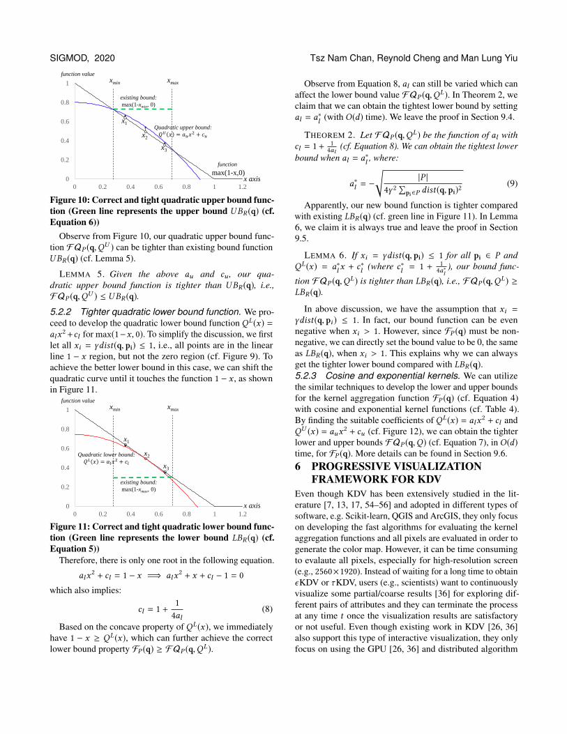
5.2.1 Tighter quadratic upper bound function. To en-sure QU (x) to be the correct and tight upper bound ofmax(1− x, 0), the quadratic function should pass through twopoints (xmin,max(1−xmin, 0)) and (xmax ,max(1−xmax , 0)),as shown in Figure 10.
Therefore, we can obtain the parameters au and cu by somealgebraic operations:
SIGMOD, 2020 Tsz Nam Chan, Reynold Cheng and Man Lung Yiu
0
0.2
0.4
0.6
0.8
1
0 0.2 0.4 0.6 0.8 1 1.2
xmin xmax
x1
x2
x3
function value
function
max(1-x,0)
existing bound:
max(1-xmin, 0)
x axis
Quadratic upper bound:
𝑄𝑈 𝑥 = 𝑎𝑢𝑥2 + 𝑐𝑢
Figure 10: Correct and tight quadratic upper bound func-tion (Green line represents the upper bound UBR (q) (cf.Equation 6))
Observe from Figure 10, our quadratic upper bound func-tion FQP (q,QU ) can be tighter than existing bound functionUBR (q) (cf. Lemma 5).
LEMMA 5. Given the above au and cu , our qua-dratic upper bound function is tighter than UBR (q), i.e.,FQP (q,QU ) ≤ UBR (q).
5.2.2 Tighter quadratic lower bound function. We pro-ceed to develop the quadratic lower bound function QL(x) =alx
2+cl for max(1−x, 0). To simplify the discussion, we firstlet all xi = γdist(q, pi) ≤ 1, i.e., all points are in the linearline 1 − x region, but not the zero region (cf. Figure 9). Toachieve the better lower bound in this case, we can shift thequadratic curve until it touches the function 1 − x , as shownin Figure 11.
0
0.2
0.4
0.6
0.8
1
0 0.2 0.4 0.6 0.8 1 1.2
xmin xmax
existing bound:
max(1-xmax, 0)
x1
x2
x3
function value
x axis
Quadratic lower bound:
𝑄𝐿 𝑥 = 𝑎𝑙𝑥2 + 𝑐𝑙
Figure 11: Correct and tight quadratic lower bound func-tion (Green line represents the lower bound LBR (q) (cf.Equation 5))
Therefore, there is only one root in the following equation.
alx2 + cl = 1 − x =⇒ alx
2 + x + cl − 1 = 0which also implies:
cl = 1 +14al
(8)
Based on the concave property of QL(x), we immediatelyhave 1 − x ≥ QL(x), which can further achieve the correctlower bound property FP (q) ≥ FQP (q,QL).
Observe from Equation 8, al can still be varied which canaffect the lower bound value FQP (q,QL). In Theorem 2, weclaim that we can obtain the tightest lower bound by settingal = a∗l (with O(d) time). We leave the proof in Section 9.4.
THEOREM 2. Let FQP (q,QL) be the function of al withcl = 1+ 1
4al (cf. Equation 8). We can obtain the tightest lowerbound when al = a∗l , where:
a∗l = −
√|P |
4γ 2 ∑pi∈P dist(q, pi)
2 (9)
Apparently, our new bound function is tighter comparedwith existing LBR (q) (cf. green line in Figure 11). In Lemma6, we claim it is always true and leave the proof in Section9.5.
LEMMA 6. If xi = γdist(q, pi) ≤ 1 for all pi ∈ P andQL(x) = a∗l x + c∗l (where c∗l = 1 + 1
4a∗l), our bound func-
tion FQP (q,QL) is tighter than LBR (q), i.e., FQP (q,QL) ≥
LBR (q).
In above discussion, we have the assumption that xi =γdist(q, pi ) ≤ 1. In fact, our bound function can be evennegative when xi > 1. However, since FP (q) must be non-negative, we can directly set the bound value to be 0, the sameas LBR (q), when xi > 1. This explains why we can alwaysget the tighter lower bound compared with LBR (q).5.2.3 Cosine and exponential kernels. We can utilizethe similar techniques to develop the lower and upper boundsfor the kernel aggregation function FP (q) (cf. Equation 4)with cosine and exponential kernel functions (cf. Table 4).By finding the suitable coefficients of QL(x) = alx
2 + cl andQU (x) = aux
2 + cu (cf. Figure 12), we can obtain the tighterlower and upper bounds FQP (q,Q) (cf. Equation 7), in O(d)time, for FP (q). More details can be found in Section 9.6.6 PROGRESSIVE VISUALIZATION
FRAMEWORK FOR KDVEven though KDV has been extensively studied in the lit-erature [7, 13, 17, 54–56] and adopted in different types ofsoftware, e.g. Scikit-learn, QGIS and ArcGIS, they only focuson developing the fast algorithms for evaluating the kernelaggregation functions and all pixels are evaluated in order togenerate the color map. However, it can be time consumingto evalaute all pixels, especially for high-resolution screen(e.g., 2560×1920). Instead of waiting for a long time to obtainϵKDV or τKDV, users (e.g., scientists) want to continuouslyvisualize some partial/coarse results [36] for exploring dif-ferent pairs of attributes and they can terminate the processat any time t once the visualization results are satisfactoryor not useful. Even though existing work in KDV [26, 36]also support this type of interactive visualization, they onlyfocus on using the GPU [26, 36] and distributed algorithm
QUAD: Quadratic-Bound-based Kernel Density Visualization SIGMOD, 2020
0
0.2
0.4
0.6
0.8
1
0 0.5 1 1.5 2
function value xminxmax
𝑄𝐿 𝑥 = 𝑎𝑙𝑥2 + 𝑐𝑙
function: cos 𝑥
existing lower bound:
cos xmax
x axis
𝑄𝑈 𝑥 = 𝑎𝑢𝑥2 + 𝑐𝑢
existing upper bound:
cos xmin
0
0.2
0.4
0.6
0.8
1
0 0.5 1 1.5 2
x axis
function: exp(−𝑥)
xmin xmax
existing lower bound:
𝑒𝑥𝑝 −xmax
existing upper bound:
𝑒𝑥𝑝 −xmin
𝑄𝐿 𝑥 = 𝑎𝑙𝑥2 + 𝑐𝑙
𝑄𝑈 𝑥 = 𝑎𝑢𝑥2 + 𝑐𝑢
function value
(a) Quadratic bounds for cos(x) (b) Quadratic bounds for exp(−x)
Figure 12: Quadratic bounds for cosine and exponential kernel functions
[36] to achieve real-time performance. In this section, weshow that, by considering the proper pixel evaluation order,the progressive visualization framework can achieve high vi-sualization quality in single machine setting without usingGPU and parallel computation, even though the time t is verysmall.
To simplify the discussion, we assume the resolution forthe visualized region is 2r × 2r , where r is the positive integer.However, our method can also handle all other resolutions.Instead of using row/column-major order to evaluate densityvalue of each pixel in the visualized region, we adopt thequad-tree like order [12] to perform the evaluation since twoclose spatial coordinates normally have similar KDE value (cf.Figure 1). Initially, our algorithm evaluates the approximateKDE value (e.g., ϵ = 0.01) in the central pixel (cf. (1) inFigure 13) as an approximation in the whole region. Then, ititeratively evaluates more density values ((2), (3), (4), (5)... inFigure 13) when more time is provided. Our algorithm stopsonce the user terminates the process or all density values(pixels) are evaluated.
…
1 1 2 2 4 4
(1)
(2) (3)
(4) (5)
Figure 13: A progressive approach to evaluate the densityvalue of each pixel (blue) in the visualized region (with or-der (1), (2),...), each density value of blue pixels representsthe density value in the corresponding sub-region, exceptfor red pixels, in which the density values have been eval-uated.
7 EXPERIMENTAL EVALUATIONWe first introduce the experimental setting in Section 7.1.Later, we demonstrate the efficiency performance in differentmethods for ϵKDV and τKDV in Section 7.2. After that, we
compare the tightness of the state-of-the-art bound functionsKARL and our proposal QUAD in Section 7.3. Next, we pro-vide the quality comparison with QUAD and other methods inSection 7.4. Then, we demonstrate the quality performance ofprogressive visualization framework with different methodsin Section 7.5. After that, we test the efficiency performancefor other kernel functions (e.g., triangular and cosine kernelfunctions) in Section 7.6. Lastly, we further test whether oursolution QUAD can still be efficient, compared with othermethods, for general kernel density estimation, with higherdimensions in Section 7.7.7.1 Experimental SettingWe use four large-scale real datasets (up to 7M) for conduct-ing the experiments, as shown in Table 5. In the followingexperiments, we choose two attributes for each dataset forvisualization. We adopt the Scott’s rule [7, 13] to obtain theparameter γ and the weighting parameter w . By default, weset the resolution to be 1280 × 960. In addition, we focus onGaussian kernel function in Sections 7.2-7.5, 7.7 and otherkernel functions in Section 7.6.
Table 5: DatasetsName n Selected attributes (2d)
El nino [2] 178080 sea surface temperature (depth=0/500)crime [1] 270688 latitude/longitudehome [2] 919438 temperature/humidityhep [2] 7000000 1st /2nd dimensions
In our experimental study, we compare different state-of-the-art methods with our solution, as shown in Table 6. EX-ACT is the sequential scan method, which does not adopt anyefficient algorithm. Scikit-learn (abbrev. Scikit) [35] is themachine learning software which can also support ϵKDV. Z-order [54, 55] is the state-of-the-art dataset sampling methodwhich provides probabilistic error guarantee for ϵKDV. tKDC[13] and aKDE [17] are indexing-based methods for τKDVand ϵKDV respectively. In the offline stage, they pre-buildone index, e.g., kd-tree, on the dataset. Each index node stores
SIGMOD, 2020 Tsz Nam Chan, Reynold Cheng and Man Lung Yiu
the information, e.g., bounding rectangles, for the bound func-tions. This approach facilitates the bound evaluations in theonline stage. Both KARL [7] and this paper also follow thisapproach and utilize the indexing structure to provide speedupfor bound evaluations. The main difference between our workQUAD and existing work aKDE, tKDC and KARL is thenewly developed tighter bound functions. We implementedall methods in C++ (except for Scikit, which is originallyimplemented in Python) and conducted experiments on anIntel i7 3.4GHz PC using Ubuntu. In this paper, we use theresponse time (sec) to measure the efficiency of all methodsand only report the response time which is smaller than 7200sec (i.e., 2 hours).
Table 6: Existing methods for two variants of KDVType EXACT Scikit Z-Order aKDE tKDC KARL QUAD
[35] [54, 55] [17] [13] [7] (ours)ϵKDV X X X X × X XτKDV X × × × X X X
7.2 Efficiency for ϵKDV and τKDVIn this section, we investigate the following four researchquestions of efficiency issues for ϵKDV and τKDV.
(1) How does the relative error ϵ affect the efficiency per-formance of all methods in ϵKDV?
(2) How does the threshold τ affect the efficiency perfor-mance of all methods in τKDV?
(3) How scalable can QUAD achieve in different resolu-tions compared with all other existing methods?
(4) How scalable can QUAD achieve in different datasetsizes compared with all other existing methods?
As a remark, both EXACT and Scikit always run out oftime (> 7200 sec). Therefore, these two curves are not shownin most of the following experimental figures.Varying ϵ for ϵKDV:
We vary the relative error ϵ for ϵKDV from 0.01 to 0.05.Figure 14 shows the response time of all methods. Eventhough Z-Order method downsamples the original datasetto the small scale dataset, they still need to evaluate the ex-act KDE (EXACT) in this reduced dataset for each pixel.Therefore, the evaluation time is still long compared withour method QUAD. On the other hand, due to the superiortightness for our bounds compared with the state-of-the-artbound functions (cf. Sections 4.2 and 4.3), QUAD can pro-vide another one order of magnitude speedup compared withKARL. Even though we choose the relative error ϵ to be 0.01,which is very small, QUAD can achieve 100-400 sec for eachlarge-scale dataset in a single machine.Varying τ for τKDV:
In order to test the efficiency performance for τKDV, weselect seven thresholds (µ−0.3σ , µ−0.2σ , µ−0.1σ , µ, µ+0.1σ ,µ + 0.2σ , µ + 0.3σ ) for each dataset, where:
µ =
∑q∈Q FP (q)
|Q |and σ =
√∑q∈Q (FP (q) − µ)2
|Q |
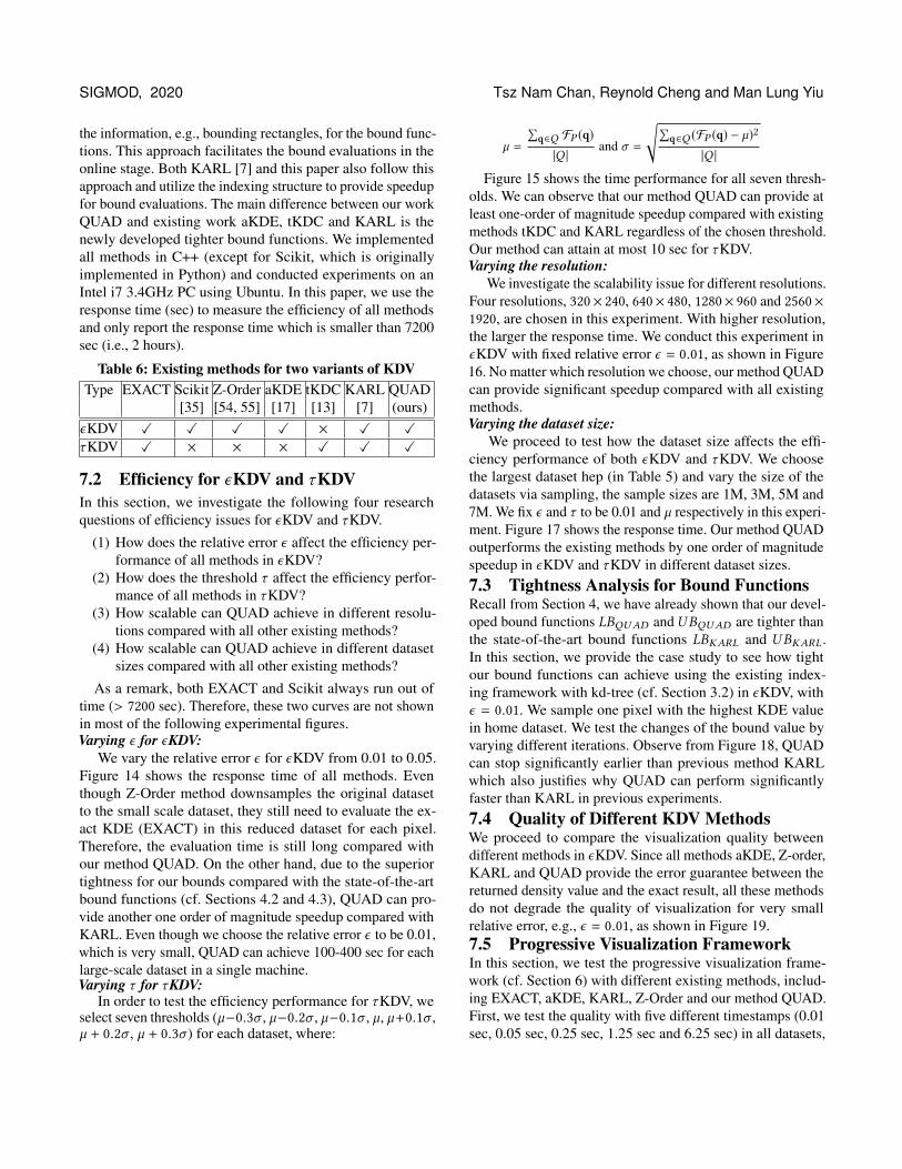
Figure 15 shows the time performance for all seven thresh-olds. We can observe that our method QUAD can provide atleast one-order of magnitude speedup compared with existingmethods tKDC and KARL regardless of the chosen threshold.Our method can attain at most 10 sec for τKDV.Varying the resolution:
We investigate the scalability issue for different resolutions.Four resolutions, 320× 240, 640× 480, 1280× 960 and 2560×1920, are chosen in this experiment. With higher resolution,the larger the response time. We conduct this experiment inϵKDV with fixed relative error ϵ = 0.01, as shown in Figure16. No matter which resolution we choose, our method QUADcan provide significant speedup compared with all existingmethods.Varying the dataset size:
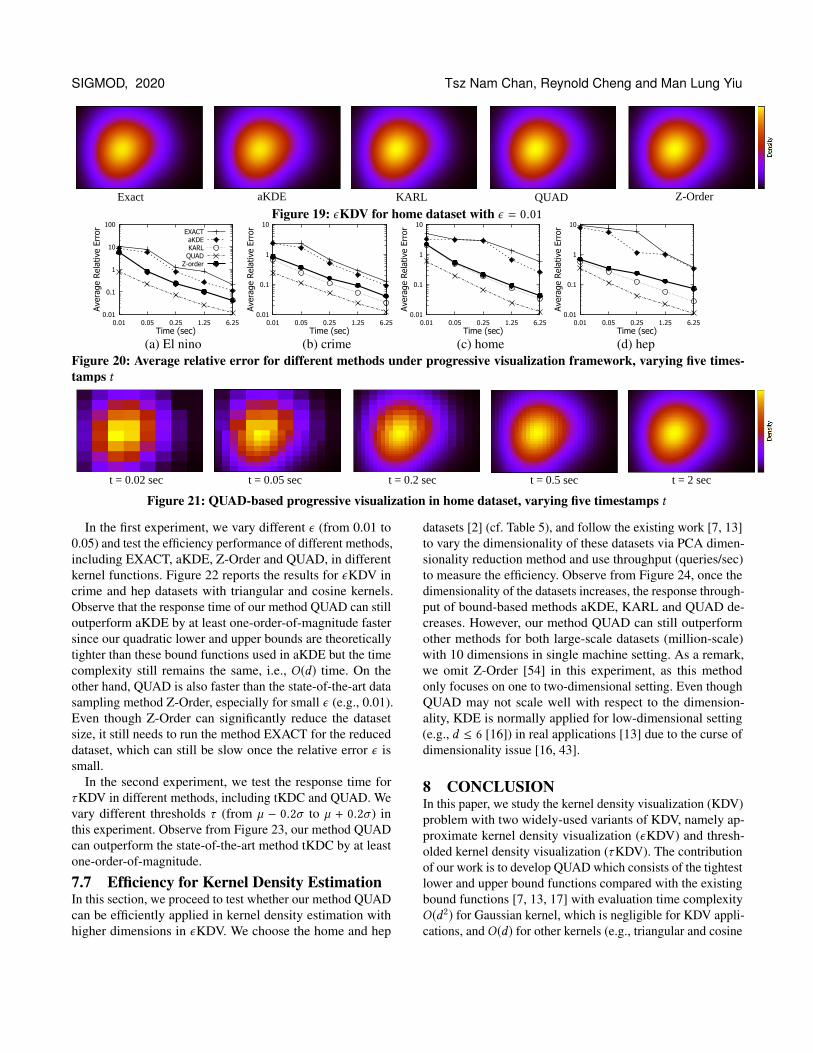
We proceed to test how the dataset size affects the effi-ciency performance of both ϵKDV and τKDV. We choosethe largest dataset hep (in Table 5) and vary the size of thedatasets via sampling, the sample sizes are 1M, 3M, 5M and7M. We fix ϵ and τ to be 0.01 and µ respectively in this experi-ment. Figure 17 shows the response time. Our method QUADoutperforms the existing methods by one order of magnitudespeedup in ϵKDV and τKDV in different dataset sizes.7.3 Tightness Analysis for Bound FunctionsRecall from Section 4, we have already shown that our devel-oped bound functions LBQUAD and UBQUAD are tighter thanthe state-of-the-art bound functions LBKARL and UBKARL .In this section, we provide the case study to see how tightour bound functions can achieve using the existing index-ing framework with kd-tree (cf. Section 3.2) in ϵKDV, withϵ = 0.01. We sample one pixel with the highest KDE valuein home dataset. We test the changes of the bound value byvarying different iterations. Observe from Figure 18, QUADcan stop significantly earlier than previous method KARLwhich also justifies why QUAD can perform significantlyfaster than KARL in previous experiments.7.4 Quality of Different KDV MethodsWe proceed to compare the visualization quality betweendifferent methods in ϵKDV. Since all methods aKDE, Z-order,KARL and QUAD provide the error guarantee between thereturned density value and the exact result, all these methodsdo not degrade the quality of visualization for very smallrelative error, e.g., ϵ = 0.01, as shown in Figure 19.7.5 Progressive Visualization FrameworkIn this section, we test the progressive visualization frame-work (cf. Section 6) with different existing methods, includ-ing EXACT, aKDE, KARL, Z-Order and our method QUAD.First, we test the quality with five different timestamps (0.01sec, 0.05 sec, 0.25 sec, 1.25 sec and 6.25 sec) in all datasets,
QUAD: Quadratic-Bound-based Kernel Density Visualization SIGMOD, 2020
1
10
100
1000
10000
0.01 0.02 0.03 0.04 0.05
Tim
e (s
ec)
ε
aKDEKARL
QUADZ-order
1
10
100
1000
10000
0.01 0.02 0.03 0.04 0.05
Tim
e (s
ec)
ε
1
10
100
1000
10000
0.01 0.02 0.03 0.04 0.05
Tim
e (s
ec)
ε
1
10
100
1000
10000
0.01 0.02 0.03 0.04 0.05
Tim
e (s
ec)
ε
(a) El nino (b) crime (c) home (d) hep
Figure 14: Response time for ϵKDV with resolution 1280 × 960, varying the relative error ϵ
1
10
100
1000
μ-0.2σ μ-0.1σ μ μ+0.1σ μ+0.2σ
Tim
e (s
ec)
τ
tKDCKARL
QUAD 1
10
100
1000
10000
μ-0.2σ μ-0.1σ μ μ+0.1σ μ+0.2σ
Tim
e (s
ec)
τ
1
10
100
1000
10000
μ-0.2σ μ-0.1σ μ μ+0.1σ μ+0.2σ
Tim
e (s
ec)
τ
1
10
100
1000
μ-0.2σ μ-0.1σ μ μ+0.1σ μ+0.2σ
Tim
e (s
ec)
τ
(a) El nino (b) crime (c) home (d) hep
Figure 15: Response time for τKDV with resolution 1280 × 960, varying the threshold τ
1
10
100
1000
10000
320x240 640x480 1280x960 2560x1920
Tim
e (s
ec)
Resolution
aKDEKARL
QUADZ-order
1
10
100
1000
10000
320x240 640x480 1280x960 2560x1920
Tim
e (s
ec)
Resolution
1
10
100
1000
10000
320x240 640x480 1280x960 2560x1920
Tim
e (s
ec)
Resolution
1
10
100
1000
10000
320x240 640x480 1280x960 2560x1920
Tim
e (s
ec)
Resolution
(a) El nino (b) crime (c) home (d) hep
Figure 16: Response time for ϵKDV with fixed relative error ϵ = 0.01, varying the resolution
1
10
100
1000
10000
1 3 5 7
Tim
e (s
ec)
Dataset size (x106)
aKDEKARL
QUADZ-order
1
10
100
1000
10000
1 3 5 7
Tim
e (s
ec)
Dataset size (x106)
tKDCKARL
QUAD
(a) ϵKDV (b) τKDVFigure 17: Response time for ϵKDV with ϵ = 0.01 andτKDV with τ = µ in hep dataset, varying the dataset size
012345678
0 20 40 60 80 100 120 140 160 180 200
QUAD stops KARL stops
Boun
d Va
lue
(x10
5 )
Iteration
LBKARLUBKARL
LBQUADUBQUAD
Figure 18: Bound values of KARL and QUAD v.s. thenumber of iterations in ϵKDV, ϵ = 0.01, in home dataset
as shown in Figure 20. We use the average relative error1|Q |
∑q∈Q
|R(q)−FP (q) |FP (q)
for the quality measure, where R(q) isthe returned result of pixel q. For each approximation method,we select the relative error parameter ϵ = 0.01. In this exper-iment, we fix the resolution to be 1280 × 960. Since QUADis faster than all other methods, it can evaluate more pixelsunder the same time limit t . Therefore, it explains why theaverage relative error is smaller than other methods with thesame t .
Figure 21 shows five visualization figures, which corre-spond to five timestamps (0.02 sec, 0.05 sec, 0.2 sec, 0.5 secand 2 sec), in home dataset with our best method QUAD. Wecan notice that once the time t is set to be 0.5 sec, QUAD canalready be able to produce the reasonable visualization result.
7.6 Efficiency for Other Kernel FunctionsIn this section, we conduct the efficiency experiments forother kernel functions, as stated in Table 4. Recall from Sec-tion 5.1, KARL [7] cannot provide the efficient linear boundsfor these kernel functions. Therefore, we omit the comparisonof this method in this section. We only report the results fortriangular and cosine kernel functions in this section. Someadditional experiment results are reported in Section 9.7.
SIGMOD, 2020 Tsz Nam Chan, Reynold Cheng and Man Lung Yiu
Exact KARLaKDE QUAD Z-Order
Figure 19: ϵKDV for home dataset with ϵ = 0.01
0.01
0.1
1
10
100
0.01 0.05 0.25 1.25 6.25
Aver
age
Rel
ativ
e Er
ror
Time (sec)
EXACTaKDEKARL
QUADZ-order
0.01
0.1
1
10
0.01 0.05 0.25 1.25 6.25
Aver
age
Rel
ativ
e Er
ror
Time (sec)
0.01
0.1
1
10
0.01 0.05 0.25 1.25 6.25
Aver
age
Rel
ativ
e Er
ror
Time (sec)
0.01
0.1
1
10
0.01 0.05 0.25 1.25 6.25
Aver
age
Rel
ativ
e Er
ror
Time (sec)
(a) El nino (b) crime (c) home (d) hepFigure 20: Average relative error for different methods under progressive visualization framework, varying five times-tamps t
t = 0.02 sec t = 0.05 sec t = 0.2 sec t = 0.5 sec t = 2 sec
Figure 21: QUAD-based progressive visualization in home dataset, varying five timestamps t
In the first experiment, we vary different ϵ (from 0.01 to0.05) and test the efficiency performance of different methods,including EXACT, aKDE, Z-Order and QUAD, in differentkernel functions. Figure 22 reports the results for ϵKDV incrime and hep datasets with triangular and cosine kernels.Observe that the response time of our method QUAD can stilloutperform aKDE by at least one-order-of-magnitude fastersince our quadratic lower and upper bounds are theoreticallytighter than these bound functions used in aKDE but the timecomplexity still remains the same, i.e., O(d) time. On theother hand, QUAD is also faster than the state-of-the-art datasampling method Z-Order, especially for small ϵ (e.g., 0.01).Even though Z-Order can significantly reduce the datasetsize, it still needs to run the method EXACT for the reduceddataset, which can still be slow once the relative error ϵ issmall.
In the second experiment, we test the response time forτKDV in different methods, including tKDC and QUAD. Wevary different thresholds τ (from µ − 0.2σ to µ + 0.2σ ) inthis experiment. Observe from Figure 23, our method QUADcan outperform the state-of-the-art method tKDC by at leastone-order-of-magnitude.
7.7 Efficiency for Kernel Density EstimationIn this section, we proceed to test whether our method QUADcan be efficiently applied in kernel density estimation withhigher dimensions in ϵKDV. We choose the home and hep
datasets [2] (cf. Table 5), and follow the existing work [7, 13]to vary the dimensionality of these datasets via PCA dimen-sionality reduction method and use throughput (queries/sec)to measure the efficiency. Observe from Figure 24, once thedimensionality of the datasets increases, the response through-put of bound-based methods aKDE, KARL and QUAD de-creases. However, our method QUAD can still outperformother methods for both large-scale datasets (million-scale)with 10 dimensions in single machine setting. As a remark,we omit Z-Order [54] in this experiment, as this methodonly focuses on one to two-dimensional setting. Even thoughQUAD may not scale well with respect to the dimension-ality, KDE is normally applied for low-dimensional setting(e.g., d ≤ 6 [16]) in real applications [13] due to the curse ofdimensionality issue [16, 43].
8 CONCLUSIONIn this paper, we study the kernel density visualization (KDV)problem with two widely-used variants of KDV, namely ap-proximate kernel density visualization (ϵKDV) and thresh-olded kernel density visualization (τKDV). The contributionof our work is to develop QUAD which consists of the tightestlower and upper bound functions compared with the existingbound functions [7, 13, 17] with evaluation time complexityO(d2) for Gaussian kernel, which is negligible for KDV appli-cations, and O(d) for other kernels (e.g., triangular and cosine
QUAD: Quadratic-Bound-based Kernel Density Visualization SIGMOD, 2020
1
10
100
1000
10000
0.01 0.02 0.03 0.04 0.05
Tim
e (s
ec)
ε
aKDEQUAD
Z-order 1
10
100
1000
10000
0.01 0.02 0.03 0.04 0.05
Tim
e (s
ec)
ε
1
10
100
1000
10000
0.01 0.02 0.03 0.04 0.05
Tim
e (s
ec)
ε
1
10
100
1000
10000
0.01 0.02 0.03 0.04 0.05
Tim
e (s
ec)
ε
(a) crime (triangular) (b) hep (triangular) (c) crime (cosine) (d) hep (cosine)
Figure 22: Response time for different methods in crime and hep datasets, varying the relative error ϵ and using trian-gular and cosine kernel functions
1
10
100
1000
μ-0.2σ μ-0.1σ μ μ+0.1σ μ+0.2σ
Tim
e (s
ec)
τ
tKDCQUAD
1
10
100
1000
10000
μ-0.2σ μ-0.1σ μ μ+0.1σ μ+0.2σ
Tim
e (s
ec)
τ
1
10
100
1000
μ-0.2σ μ-0.1σ μ μ+0.1σ μ+0.2σ
Tim
e (s
ec)
τ
1
10
100
1000
10000
μ-0.2σ μ-0.1σ μ μ+0.1σ μ+0.2σ
Tim
e (s
ec)
τ
(a) crime (triangular) (b) hep (triangular) (c) crime (cosine) (d) hep (cosine)
Figure 23: Response time for different methods in crime and hep datasets, varying the threshold τ and using triangularand cosine kernel functions
1
10
100
1000
10000
2 4 6 8 10
Thro
ughp
ut (
Que
ries/
sec)
dimensionality
SCANaKDEKARL
QUAD
0.1
1
10
100
1000
10000
100000
2 4 6 8 10
Thro
ughp
ut (
Que
ries/
sec)
dimensionality
(a) home (b) hep
Figure 24: Response throughput (queries/sec) for differ-ent methods in home and hep datasets (with Gaussiankernel and ϵ = 0.01), varying the dimensionality
kernels). Our method QUAD can provide at least one-order-of-magnitude speedup compared with different state-of-the-artmethods under small relative error ϵ and different thresholdsτ . The combination of QUAD and progressive visualizationframework can further provide reasonable visualization re-sults with real-time performance (0.5 sec) in single machinesetting without using GPU and parallel computation.
In the future, we will further apply QUAD to other kernel-based machine learning models, e.g., kernel regression, kernelSVM and kernel clustering. Moreover, we will explore theoppontunity to utilize the parallel/distributed computation[54] and modern hardware [16, 52] to further speed up oursolution.
9 APPENDIX9.1 Proof of Lemma 2
PROOF. We only prove the upper bound FP (q) ≤
FQP (q,QU ) but it can be extended to lower bound in a
straightforward way. We first substitute x = γdist(q, pi)2 inthe following inequality, exp(−x) ≤ QU (x) = aux
2+bux +cu .Then, we have:
exp(−γdist(q, pi)2) ≤ au (γdist(q, pi)2)2+buγdist(q, pi)2+cu
By taking the summation in both sides with respect to eachpi ∈ P and then multiplying both sides with the constant w ,we can prove FP (q) ≤ FQP (q,QU ). �
9.2 Proof of Lemma 3PROOF. From Equation 2, we have:
pi∈P | |pi | |4. All of these terms only depend onP and can be computed once and stored when we build theindexing structure (cf. Figure 3). As such, the first five termscan be computed in O(d) time in the query stage. We nowshow that the last term can be computed in O(d2) time.∑pi∈P
(qT pi)2 =∑pi∈P
(qT pi)(piT q) = qT( ∑pi∈P
pipiT)q = qTCq
SIGMOD, 2020 Tsz Nam Chan, Reynold Cheng and Man Lung Yiu
where C is the matrix which depends on P and can be com-puted when we build the indexing structure.
In the query stage, the computation time of qTCq isin O(d2) time. Hence, the time complexity for evaluatingFQP (q,Q) is O(d2). �
9.3 Proof of Theorem 1PROOF. We first investigate the slope (1st derivative)
curves of both exp(−x) and QU (x) = aux2 + bux + cu which
are − exp(−x) and 2aux +bu respectively, as shown in Figure25.
-1
-0.8
-0.6
-0.4
-0.2
0
0.2
0 1 2 3 4
slope value
1st derivative:
−exp(−𝑥)
𝑑𝑄𝑈(𝑥)
𝑑𝑥= 2𝑎𝑢𝑥 + 𝑏𝑢
Region I Region II Region III
Figure 25: The slope curves of both QU (x) and exp(−x)In general, 2aux + bu may not intersect with − exp(−x) by
two points. However, it is impossible here. Once the slope ofQU (x) is always larger than the slope of exp(−x), QU (x) andexp(−x) can only intersect with at most one point. However,QU (x) must intersect with exp(−x) by (xmin, exp(−xmin)) and(xmax, exp(−xmax)), which leads to contradiction. As such,2aux + bu must intersect with − exp(−x) by two points.
Observe from Figure 25, the slope of one curve is alwayslarger than another one in each region. Therefore, once theyhave the intersection point in this region, they must not haveanother intersection point again in this region as one curvealways move “faster” than another one.
LEMMA 7. For each region in Figure 25, there is at mostone intersection point in exp(−x) and QU (x).
Once we have Lemma 7, we can use it to prove this theorem(correctness and tightness).
Correct upper bound for our chosen a∗u : Observe from Fig-ure 7, we have two conditions for the correct upper boundfunction.
• The slope of quadratic function dQU (x )dx at the point
(xmax, exp(−xmax)) must be more negative than theslope of exp(−x).
• There is no other intersection point, except(xmin, exp(−xmin)) and (xmax, exp(−xmax)), forthe functions exp(−x) and QU (x) in the interval[xmin, xmax].
Based on the first condition, xmax must be in region II inFigure 25. By Lemma 7, xmin can only be in region I and
there is no other intersection point between xmin and xmax,which fulfills the second condition. Therefore, we conclude:
LEMMA 8. IfQU (x) is the proper upper bound of exp(−x),xmax must be in region II.
Since xmax must be in region II, we have:dQU (x)
dx
���x=xmax
≤ − exp(−xmax)
2auxmax + bu ≤ − exp(−xmax)
By substituting bu in terms of the function of au (cf. Section4.2), we have au ≤ a∗u . Therefore, our selected a∗u is withinthis region and hence it achieves correct upper bound function.
The tighter upper bound for our chosen au = a∗u : To provethis part, we substitute bu and cu with respect to au intoQU (x) = aux
2 + bux + cu . Then, we have:
QU (x) = au (x − xmin)(x − xmax) +mux + ku
where mu and ku are the slope and intercept, respec-tively, of the linear line (chord) which passes through(xmin, exp(−xmin)) and (xmax, exp(−xmax)).
Note that only the first term in QU (x) depends on au andthe term (x − xmin)(x − xmax) < 0 for every x in the range[xmin, xmax]. Since au > 0, QU (x) is smaller once au is larger,and thus the upper bound is tighter. However, as stated inthe correctness proof, the largest possible au should be a∗u .Hence, we can achieve the tighter bound once au = a∗u , sincethe linear function mux + ku is in fact the special case ofQU (x) with au = 0 ≤ a∗u . �
9.4 Proof of Theorem 2PROOF. Let H (al ) = FQP (q,QL), we have:
H (al ) =∑pi∈P
w(al (γdist(q, pi))
2 +(1 +
14al
))dH (al )
dal= wγ 2
∑pi∈P
dist(q, pi)2 −w |P |
4a2l
By setting dH (al )dal
= 0, we can obtain:
al = a∗l = −
√|P |
4γ 2∑pi∈P dist(q, pi)
2
Based on the basic differentiation theory, we conclude thatal = a∗l can achieve the maximum for FQP (q,QL). �
9.5 Proof of Lemma 6PROOF. By substituting a∗l (cf. Equation 9) and c∗l (cf.
Equation 8) in FQP (q,QL) (cf. Equation 7), we can obtain:
FQP (q,QL) = w |P | −w
√|P |
∑pi∈P
(γdist(q, pi))2
≥ w |P |(1 − xmax) = LBR (q)
The last equality is based on the assumption xi =γdist(q, pi) ≤ 1. �
QUAD: Quadratic-Bound-based Kernel Density Visualization SIGMOD, 2020
9.6 Correct and Tight Quadratic Bounds forCosine and Exponential Kernel Functions
Recall from Section 5.2.3, we can obtain the correct and tightlower and upper bound functions for FP (q) (cf. Equation4), if we can find the suitable parameters al , cl and au , curespectively. In this section, we illustrate how to obtain theseparameters in order to achieve the correct and tight quadraticbounds.
9.6.1 Quadratic upper bound for cosine kernel. Ob-serve from Figure 12a, once QU (x) (blue curve) passesthrough two points (xmin, cos(xmin)) and (xmax, cos(xmax)), itis possible for this curve to act as the upper bound function forcos(x). Therefore, by simple algebraic operations, we have:
au =cos(xmax) − cos(xmin)
x2max − x2min(10)
cu =x2max cos(xmin) − x2min cos(xmax)
x2max − x2min(11)
In Lemma 9, we formally show that QU (x) can act as thecorrect upper bound for cos(x), using the above au and cu .
LEMMA 9. If we set au and cu to be Equations 10 and 11respectively, we have QU (x) ≥ cos(x), where 0 ≤ x ≤ π
2 .
PROOF. We let H (x) = aux2 + cu − cos(x). Since we set
au and cu to be Equations 10 and 11, it implies:
H (xmin) = 0 and H (xmax) = 0
To prove the correctness of this lemma, we need to ensureH (x) ≥ 0 if 0 ≤ x ≤ π
2 . We first compute the derivation ofH (x):
dH (x)
dx= 2aux + sin(x) = x
(2au +
sin(x)x
)Then, we set dH (x )
dx
���x=x ∗
= 0 in order to achieve local opti-mal for H (x), i.e.
sin(x∗)x∗
= −2au
We plot the sin(x )x function and its possible local optimal
point in Figure 26. Observe that this function is monotonicdecreasing function for 0 ≤ x ≤ π . There are three possiblecases for the positions of xmin and xmax.
Case 1 (xmax ≤ x∗): Observe from Figure 26, we noticethat sin(x )
x > −2au since x ≤ xmax ≤ x∗. Therefore, we havedH (x )dx > 0, i.e. H (x) is monotonic increasing function. We
can conclude H (x) ≥ H (xmin) = 0.Case 2 (xmin ≥ x∗): Using the similar technique as Case 1,
we conclude sin(x )x < −2au . As such H (x) is the monotonic
decreasing function. Therefore, H (x) ≥ H (xmax) = 0.Case 3 (xmin ≤ x ≤ xmax): Observe from Figure 26,
sin(x )x ≥ −2au when x ≤ x∗ and sin(x )
x ≤ −2au when x ≥ x∗,
0
0.2
0.4
0.6
0.8
1
1.2
0 0.5 1 1.5 2 2.5 3 3.5
function: sin 𝑥
𝑥
-2au(x*,-2au)
function value
Figure 26: The function sin(x )x
we conclude that x∗ is the local maximum, the global mini-mum point can be achieved in the extreme points, i.e. xminand xmax. Therefore, H (x) ≥ min(H (xmin),H (xmax)) = 0. Weconclude QU (x) = aux + cu ≥ cos(x). �
Since QU (x) is the monotonic decreasing function andQU (xmin) = cos(xmin), we can also show that QU (x) ≤
cos(xmin), given xmin ≤ x ≤ xmax, i.e., QU (x) is alwaystighter than the state-of-the-art bound function cos(xmin) (cf.Figure 12a).
9.6.2 Quadratic lower bound for cosine kernel. Toachieve the correct lower bound for cosine kernel, we restrictthe quadratic curve to pass though the point (xmax, cos(xmax))in which the slope of two curves are the same at this point(cf. Figure 12a). Therefore, by simple algebraic and calculusoperations, we obtain:
al =− sin(xmax)
2xmax(12)
cl = cos(xmax) +xmax sin(xmax)
2(13)
Now, we claim that the quadratic function can achieve thecorrect lower bound functions by using the above al and cl(cf. Lemma 10).
LEMMA 10. If we set al and cl to be Equations 12 and 13respectively, we have QL(x) ≤ cos(x), where 0 ≤ x ≤ π
2 .
PROOF. We let H (x) = ax2 + c − cos(x). Recall from Fig-ure 26, the maximum point, for 0 ≤ x ≤ π
2 is x∗, wheredH (x )dx
���x=x ∗
= 0. However, we notice that:
dQL(x)
dx
���x=xmax
= − sin(xmax) ⇐⇒dH (x)
dx
���x=x ∗
= 0
Therefore, we have x∗ = xmax. As such, H (x) ≤ H (xmax) = 0which implies QL(x) ≤ cos(x). �
SIGMOD, 2020 Tsz Nam Chan, Reynold Cheng and Man Lung Yiu
Since QL(x) is the monotonic decreasing function andQL(xmax) = cos(xmax), we have QL(x) ≥ cos(xmax), givenxmin ≤ x ≤ xmax. Therefore, we show that QL(x) is tighterthan the state-of-the-art bound function cos(xmax).
9.6.3 Quadratic upper bound for exponential kernel.Observe from Figure 12b, once the quadratic function QU (x)(blue curve) passes through two points (xmin, exp(−xmin)) and(xmax, exp(−xmax)), it is possible for QU (x) to act as the cor-rect upper bound for exp(−x), given xmin ≤ x ≤ xmax. There-fore, by simple algebraic operations, we can obtain:
au =exp(−xmax) − exp(−xmin)
x2max − x2min(14)
cu =x2max exp(−xmin) − x2min exp(−xmax)
x2max − x2min(15)
In Lemma 11, we further show that this QU (x) can achievethe correct upper bound function, using the above parametersau and cu .
LEMMA 11. If au and cu are set to Equations 14 and 15respectively, QU (x) ≥ exp(−x).
PROOF. Note that the linear line which passes though(xmin, exp(−xmin)) and (xmax, exp(−xmax)) also acts as the up-per bound of exp(−x). Moreover, QU (x) = aux
2 + cu is theconcave function which acts as the upper bound of this linearline. Therefore, we conclude QU (x) ≥ exp(−x). �
For the tightness of the quadratic upper bound, we ob-serve that QU (x) is the monotonic decreasing function andQU (xmin) = exp(−xmin). Therefore, we can show that QU (x)is always tighter than the state-of-the-art upper bound func-tion exp(−xmin).
9.6.4 Quadratic lower bound for exponential kernel.Observe from Figure 12b, the quadratic function QL(x) =alx
2 + cl (red curve) can act as the lower bound of exp(−x)once this curve passes through the tangent point (t, exp(−t)).Therefore, we have:
al =− exp(−t)
2t(16)
cl =12(t + 2) exp(−t) (17)
In Lemma 12, we show that QL(x) can act as the correctlower bound if we choose the above parameters al and cl .
LEMMA 12. If al and cl are set to Equations 16 and 17respectively, QL(x) ≤ exp(−x).
PROOF. Since the linear line which passes through thetangent point (t, exp(−t)) also acts as the lower bound ofexp(−x) and QL(x) is the lower bound of this linear line (dueto the concave property), we can conclude QL(x) ≤ exp(−x).
�
In Equations 16 and 17, both al and cl still depend onthe tangent parameter t . We observe that once we chooset = xmax, we can show that this QL(x) can achieve the tighterlower bound compared with the state-of-the-art lower boundfunction exp(−xmax), due to the monotonic decreasing prop-erty ofQL(x) andQL(xmax) = exp(−xmax). In order to achievethe tightest lower bound, we choose the best t = t∗ (cf. Equa-tion 18):
t∗ =
√γ 2
∑pi∈P dist(q, pi)
2
|P |(18)
We omit the proof for the best t = t∗ as this is similar withthe proof in Theorem 2.
9.7 Additional experiments for exponentialkernel function
In this section, we test the efficiency performance for bothϵKDV and τKDV for exponential kernel function, which isomitted in Section 7.6. As shown in Figure 27, our methodcan at least provide one-order-of-magnitude speedup com-pared with existing methods. In Figure 27d, the state-of-the-art method tKDC is still slower than 7200 sec for all thresh-olds and thus, we do not report the response time in thisfigure.
1
10
100
1000
10000
0.01 0.02 0.03 0.04 0.05
Tim
e (s
ec)
ε
aKDEQUAD
Z-order 1
10
100
1000
10000
0.01 0.02 0.03 0.04 0.05Ti
me
(sec
)ε
(a) crime (ϵKDV) (b) hep (ϵKDV)
1
10
100
1000
10000
μ-0.2σ μ-0.1σ μ μ+0.1σ μ+0.2σ
Tim
e (s
ec)
τ
tKDCQUAD
1
10
100
1000
μ-0.2σ μ-0.1σ μ μ+0.1σ μ+0.2σ
Tim
e (s
ec)
τ
(c) crime (τKDV) (d) hep (τKDV)
Figure 27: Response time for different methods in crimeand hep datasets for ϵKDV (a and b) and τKDV (c andd), using exponential kernel function
ACKNOWLEDGEMENTWe would like to thank Zichen Zhu for the help in someof the proofs in Section 9.6. Tsz Nam Chan and ReynoldCheng were supported by the Research Grants Council ofHong Kong (RGC Projects HKU 17229116, 106150091,and 17205115), the University of Hong Kong (Projects
QUAD: Quadratic-Bound-based Kernel Density Visualization SIGMOD, 2020
104004572, 102009508, and 104004129), and the Innova-tion and Technology Commission of Hong Kong (ITF projectMRP/029/18). Man Lung Yiu was supported by grant GRF152050/19E from the Hong Kong RGC.
REFERENCES[1] Atlanta police department open data. http://opendata.atlantapd.org/.[2] UCI machine learning repository. http://archive.ics.uci.edu/ml/index.
php.[3] Comparison of density estimation methods for astronomical datasets.
Astronomy and Astrophysics, 531, 7 2011.[4] S. Chainey, L. Tompson, and S. Uhlig. The utility of hotspot mapping
for predicting spatial patterns of crime. Security Journal, 21(1):4–28,Feb 2008.
[5] T. N. Chan, M. L. Yiu, and K. A. Hua. A progressive approach forsimilarity search on matrix. In SSTD, pages 373–390. Springer, 2015.
[6] T. N. Chan, M. L. Yiu, and K. A. Hua. Efficient sub-window nearestneighbor search on matrix. IEEE Trans. Knowl. Data Eng., 29(4):784–797, 2017.
[7] T. N. Chan, M. L. Yiu, and L. H. U. KARL: fast kernel aggregationqueries. In ICDE, pages 542–553, 2019.
[8] W. Chen, F. Guo, and F. Wang. A survey of traffic data visualiza-tion. IEEE Trans. Intelligent Transportation Systems, 16(6):2970–2984,2015.
[9] E. Cheney and W. Light. A Course in Approximation Theory. Mathe-matics Series. Brooks/Cole Publishing Company, 2000.
[10] K. Cranmer. Kernel estimation in high-energy physics. 136:198–207,2001.
[11] M. D. Felice, M. Petitta, and P. M. Ruti. Short-term predictability ofphotovoltaic production over italy. Renewable Energy, 80:197 – 204,2015.
[12] S. Frey, F. Sadlo, K. Ma, and T. Ertl. Interactive progressive visualiza-tion with space-time error control. IEEE Trans. Vis. Comput. Graph.,20(12):2397–2406, 2014.
[13] E. Gan and P. Bailis. Scalable kernel density classification via threshold-based pruning. In ACM SIGMOD, pages 945–959, 2017.
[14] E. R. Gansner, Y. Hu, S. C. North, and C. E. Scheidegger. Multilevelagglomerative edge bundling for visualizing large graphs. In PacificVis,pages 187–194, 2011.
[15] W. Gong, D. Yang, H. V. Gupta, and G. Nearing. Estimating informationentropy for hydrological data: One-dimensional case. Water ResourcesResearch, 50(6):5003–5018, 2014.
[16] A. Gramacki. Nonparametric Kernel Density Estimation and Its Compu-tational Aspects. Studies in Big Data. Springer International Publishing,2017.
[17] A. G. Gray and A. W. Moore. Nonparametric density estimation:Toward computational tractability. In SDM, pages 203–211, 2003.
[18] T. Guo, K. Feng, G. Cong, and Z. Bao. Efficient selection of geospatialdata on maps for interactive and visualized exploration. In SIGMOD,pages 567–582, 2018.
[19] T. Guo, M. Li, P. Li, Z. Bao, and G. Cong. Poisam: a system for efficientselection of large-scale geospatial data on maps. In SIGMOD, pages1677–1680, 2018.
[20] T. Hart and P. Zandbergen. Kernel density estimation and hotspotmapping: examining the influence of interpolation method, grid cellsize, and bandwidth on crime forecasting. Policing: An InternationalJournal of Police Strategies and Management, 37:305–323, 2014.
[21] Q. Jin, X. Ma, G. Wang, X. Yang, and F. Guo. Dynamics of major airpollutants from crop residue burning in mainland china, 2000–2014.Journal of Environmental Sciences, 70:190 – 205, 2018.
[22] S. C. Joshi, R. V. Kommaraju, J. M. Phillips, and S. Venkatasubrama-nian. Comparing distributions and shapes using the kernel distance. InSOCG, pages 47–56, 2011.
[23] P. K. Kefaloukos, M. A. V. Salles, and M. Zachariasen. Declarativecartography: In-database map generalization of geospatial datasets. InICDE, pages 1024–1035, 2014.
[24] J. Kehrer and H. Hauser. Visualization and visual analysis of multi-faceted scientific data: A survey. IEEE Trans. Vis. Comput. Graph.,19(3):495–513, 2013.
[25] D. A. Keim. Visual exploration of large data sets. Commun. ACM,44(8):38–44, 2001.
[26] O. D. Lampe and H. Hauser. Interactive visualization of streaming datawith kernel density estimation. In PacificVis, pages 171–178, 2011.
[27] H. Lee and K. Kang. Interpolation of missing precipitation data usingkernel estimations for hydrologic modeling. Advances in Meteorology,pages 1–12, 2015.
[28] M. Li, Z. Bao, F. M. Choudhury, and T. Sellis. Supporting large-scalegeographical visualization in a multi-granularity way. In WSDM, pages767–770, 2018.
[29] Y.-P. Lin, H.-J. Chu, C.-F. Wu, T.-K. Chang, and C.-Y. Chen. Hotspotanalysis of spatial environmental pollutants using kernel density esti-mation and geostatistical techniques. International Journal of Environ-mental Research and Public Health, 8(1):75–88, 2011.
[30] Y. Ma, M. Richards, M. Ghanem, Y. Guo, and J. Hassard. Air pollu-tion monitoring and mining based on sensor grid in london. Sensors,8(6):3601–3623, 2008.
[31] A. Mayorga and M. Gleicher. Splatterplots: Overcoming overdrawin scatter plots. IEEE Transactions on Visualization and ComputerGraphics, 19(9):1526–1538, Sept 2013.
[32] L. Micallef, G. Palmas, A. Oulasvirta, and T. Weinkauf. Towardsperceptual optimization of the visual design of scatterplots. IEEE Trans.Vis. Comput. Graph., 23(6):1588–1599, 2017.
[33] Y. Park, M. J. Cafarella, and B. Mozafari. Visualization-aware samplingfor very large databases. In ICDE, pages 755–766, 2016.
[34] Y. Park, B. Mozafari, J. Sorenson, and J. Wang. Verdictdb: Universal-izing approximate query processing. In SIGMOD, pages 1461–1476,2018.
[35] F. Pedregosa, G. Varoquaux, A. Gramfort, V. Michel, B. Thirion,O. Grisel, M. Blondel, P. Prettenhofer, R. Weiss, V. Dubourg, J. Vander-Plas, A. Passos, D. Cournapeau, M. Brucher, M. Perrot, and E. Duch-esnay. Scikit-learn: Machine learning in python. Journal of MachineLearning Research, 12:2825–2830, 2011.
[36] A. Perrot, R. Bourqui, N. Hanusse, F. Lalanne, and D. Auber. Largeinteractive visualization of density functions on big data infrastructure.In LDAV, pages 99–106, 2015.
[37] J. M. Phillips. ϵ -samples for kernels. In SODA, pages 1622–1632,2013.
[38] J. M. Phillips and W. M. Tai. Improved coresets for kernel densityestimates. In SODA, pages 2718–2727, 2018.
[39] J. M. Phillips and W. M. Tai. Near-optimal coresets of kernel densityestimates. In SOCG, pages 66:1–66:13, 2018.
[40] QGIS Development Team. QGIS Geographic Information System.Open Source Geospatial Foundation, 2009.
[41] V. C. Raykar, R. Duraiswami, and L. H. Zhao. Fast computation ofkernel estimators. Journal of Computational and Graphical Statistics,19(1):205–220, 2010.
[42] A. D. Sarma, H. Lee, H. Gonzalez, J. Madhavan, and A. Y. Halevy.Efficient spatial sampling of large geographical tables. In SIGMOD,pages 193–204, 2012.
[43] D. Scott. Multivariate Density Estimation: Theory, Practice, and Visu-alization. A Wiley-interscience publication. Wiley, 1992.
SIGMOD, 2020 Tsz Nam Chan, Reynold Cheng and Man Lung Yiu
[44] A. C. Telea. Data Visualization: Principles and Practice, SecondEdition. A. K. Peters, Ltd., Natick, MA, USA, 2nd edition, 2014.
[45] L. Thakali, T. J. Kwon, and L. Fu. Identification of crash hotspots usingkernel density estimation and kriging methods: a comparison. Journalof Modern Transportation, 23(2):93–106, Jun 2015.
[46] P. Vermeesch. On the visualisation of detrital age distributions. Chemi-cal Geology, 312-313(Complete):190–194, 2012.
[47] I. A. S. Vladislav Kirillovich Dziadyk. Theory of Uniform Approxima-tion of Functions by Polynomials. Walter De Gruyter, 2008.
[48] M. Williams and T. Munzner. Steerable, progressive multidimensionalscaling. In InfoVis, pages 57–64, 2004.
[49] K. Xie, K. Ozbay, A. Kurkcu, and H. Yang. Analysis of traffic crashesinvolving pedestrians using big data: Investigation of contributing fac-tors and identification of hotspots. Risk Analysis, 37(8):1459–1476,2017.
[50] C. Yang, R. Duraiswami, and L. S. Davis. Efficient kernel machinesusing the improved fast gauss transform. In NIPS, pages 1561–1568,2004.
[51] H. Yu, P. Liu, J. Chen, and H. Wang. Comparative analysis of thespatial analysis methods for hotspot identification. Accident Analysis
and Prevention, 66:80 – 88, 2014.[52] G. Zhang, A. Zhu, and Q. Huang. A gpu-accelerated adaptive ker-
nel density estimation approach for efficient point pattern analysis onspatial big data. International Journal of Geographical InformationScience, 31(10):2068–2097, 2017.
[53] X. Zhao and J. Tang. Crime in urban areas: A data mining perspective.SIGKDD Explorations, 20(1):1–12, 2018.
[54] Y. Zheng, J. Jestes, J. M. Phillips, and F. Li. Quality and efficiency forkernel density estimates in large data. In SIGMOD, pages 433–444,2013.
[55] Y. Zheng, Y. Ou, A. Lex, and J. M. Phillips. Visualization of big spatialdata using coresets for kernel density estimates. In IEEE Symposiumon Visualization in Data Science (VDS ’17), to appear. IEEE, 2017.
[56] Y. Zheng and J. M. Phillips. L∞ error and bandwidth selection forkernel density estimates of large data. In SIGKDD, pages 1533–1542,2015.
[57] M. Zinsmaier, U. Brandes, O. Deussen, and H. Strobelt. Interactivelevel-of-detail rendering of large graphs. IEEE Trans. Vis. Comput.Graph., 18(12):2486–2495, 2012.