This Report has been prepared by RIVM, EFTEC, NTUA and IIASA in association with TME and TNO under contract with the Environment Directorate-General of the European Commission. Technical Report on Chemicals, Particulate Matter, Human Health, Air Quality and Noise RIVM report 481505015 Technical Report on Chemicals, Particulate Matter, Human Health, Air Quality and Noise W. Smeets, A. van Pul, H. Eerens, R. Sluyter, D.W. Pearce, A. Howarth, A. Visschedijk, M.P.J. Pulles, G. de Hollander May 2000 RIVM, P.O. Box 1, 3720 BA Bilthoven, telephone: 31 - 30 - 274 91 11; telefax: 31 - 30 - 274 29 71
Transcript
This Report has been prepared by RIVM, EFTEC, NTUA and IIASA in association withTME and TNO under contract with the Environment Directorate-General of the EuropeanCommission.
Technical Report on Chemicals, Particulate Matter, Human Health, Air Quality and Noise
RIVM report 481505015
Technical Report on Chemicals, Particulate Matter, HumanHealth, Air Quality and Noise
W. Smeets, A. van Pul, H. Eerens, R. Sluyter,D.W. Pearce, A. Howarth, A. Visschedijk,M.P.J. Pulles, G. de Hollander
Chemicals and particulate matterHuman health and Air quality
This Report has been prepared by RIVM, EFTEC, NTUA and IIASA in association with TME and TNO undercontract with the Environment Directorate-General of the European Commission. This report is one of a seriesof reports supporting the main report: (XURSHDQ�(QYLURQPHQWDO�3ULRULWLHV��DQ�,QWHJUDWHG�(FRQRPLF�DQG(QYLURQPHQWDO�$VVHVVPHQW. Reports in this series have been subject to limited peer review.
The report consists of four parts:Section 1: &KHPLFDOV�DQG�SDUWLFXODWH�PDWWHU
Prepared by Winand Smeets and Addo van Pul (RIVM)in close collaboration with Antoon Visschedijk and Tinus Pulles (TNO)with contributions from Drs. G.J. Reinds and Dr. W. de Vries (Alterra, The Netherlands).
Section 2: +XPDQ�KHDOWK�DQG�DLU�TXDOLW\Prepared by Hans Eerens and Rob Sluyter (RIVM);annex 3 by Guus de Hollander RIVM)
Section 3: %HQHILW�DVVHVVPHQWPrepared by D.W. Pearce, A. Howarth (EFTEC)
Section 4: 3ROLF\�DVVHVVPHQWPrepared by D.W. Pearce, A. Howarth (EFTEC)
ReferencesAll references made in the sections on benefit and policy assessment have been brought together in the7HFKQLFDO�5HSRUW�RQ 0HWKRGRORJ\��&RVW�%HQHILW�$QDO\VLV�DQG�3ROLF\�5HVSRQVHV. The references made in thesections 1 and 2 on environmental assessment follows at the end of their section.
1RWH�WR�WKH�UHDGHU�This ‘technical report’ provides background information on two issues in the main report: ‘Chemicals andparticulate matter’ and ‘Human Health and Air Quality’.There are four sections.Section 1 deals with a) emissions and costs of emission abatement of primary particulate matter and persistentorganic pollutants (POPs), such as dioxins, and b) emissions and depositions of heavy metals, which are oftenattached to primary particulate matter, and of some pesticides.Section 2 deals with air quality in urban and rural areas for a selected number of pollutants:• primary particulate matter, lead, B(a)P, and benzene and• secondary particulate matter (from SO2, NOx and NH3), and SO2, NOx, of which the emissions are dealt
with in the context of acidification and eutrophication (VHH�7HFKQLFDO�5HSRUW�$FLGLILFDWLRQ��(XWURSKLFDWLRQDQG�7URSRVSKHULF�2]RQH).
Economic Benefits with regard to human health are dealt with in Section 3, where also cost-benefit ratios(especially for particulate matter) are presented.Finally, Section 4 deals with a set of possible policy measures to reduce emissions of pollutants (VHH�VHFWLRQ��)beyond baseline levels.
The findings, conclusions, recommendations and views expressed in this report represent those of the authorsand do not necessarily coincide with those of the European Commission services.
Technical Report on Chemicals, Particulate Matter, Human Health, Air Quality and Noise
��� 0HWKRGRORJ\ �1.2.1 Emissions 81.2.2 Atmospheric transport and deposition 111.2.3 Critical loads 13
��� 5HVXOWV�DQG�DQDO\VLV ��1.3.1 Emission scenarios 141.3.2 Emissions and costs EU 181.3.3 Emissions and costs in accession countries 311.3.4 Emissions other countries 321.3.5 Depositions and critical loads 33
��� &RQFOXVLRQV ��
�� +80$1�+($/7+�$1'�$,5�32//87,21 ��
��� ,QWURGXFWLRQ ��2.1.1 Overview 392.1.2 Human health Indicators 392.1.3 Exposure indicators 402.1.4 Study outline 42
��� 0HWKRGV ��2.2.1 Emissions 422.2.2 Selected cities 432.2.3 Urban emission processing 442.2.4 Meteorological data 452.2.5 Modelling 452.2.6 Concentration calculation methodology 482.2.7 Conversion of annual means into percentiles 50
��� &RQFOXVLRQ�DQG�5HVXOWV ��2.3.1 Main trends 552.3.2 Urban Air Pollution: Road Transport Takes the Lead 55
This section on chemicals and particulate matter considers the future emission trends to air of primaryparticulate matter (PM), heavy metals (HMs) and persistent organic pollutants (POPs), and also briefly discussesdeposition for some selected HMs (cadmium, copper, lead), and POPs (dioxins/furans, atrazine, endosulfan,lindane, pentacholorophenol). In addition, impacts on forest soils are evaluated for cadmium, copper and lead.Human exposure to selected air pollutants (PM, Benz(a)Pyrene, benzene, lead) is dealt with in a separate section(VHH�VHFWLRQ��). Impacts of HMs and POPs on non-forest ecosystems have not been assessed.
Primary particulate matter consists of particles emitted from anthropogenic and natural sources such ascombustion, industrial processes, sea-salt spray and suspended soil dust. Secondary PM is formed by chemicalreaction from SO2, NOx, and NH3 gases, condensation of organic vapours emitted from various anthropogenicsources and photochemical reactions. This study uses PM10
1 as main indicator for the effects of human exposureto particulates. Emission trends presented in this section only relate to emissions from anthropogenic origin.
Chemicals are introduced into the environment through human activities. These include the release fromproduction and use, but also the dispersion as unwanted by-products during combustion and industrialprocesses. Chemicals are dispersed into the air, water and soil, and may lead to unwanted effects on humanhealth and ecosystems.
Among the large number of chemicals entering the environment, HMs and POPs represent two groups that areof particular importance due to their persistent, bio-accumulative and toxic characteristics. HMs and POPs areknown to be a threat to human health (blood and organ disorders, carcinogenic effects, birth defects, intellectualdevelopment) and the environment (forest ecosystem stress, reproductive impairment). Clearly, there are tens ofthousands of chemicals (including pesticides) that could be considered, but this study will focus on emissions ofheavy metals (HMs) and persistent organic pollutants (POPs) to air that are subject to EU, UN-ECE and otherinternational agreements and for which a reasonable amount of data exists. The environmental problems aroundchemicals (or hazardous substances) are presented in detail in the state-of-environment reports brought out bythe EEA (EEA, 1998; 1999). The risk assessments of new and existing non-assessed chemicals dealt with in EUregulations are GLVFXVVHG�LQ�%R[����.
Emission targets have been established for specific HMs and POPs under the auspices of the UN/ECEConvention on Long-Range Transboundary Air Pollution (CLRTAP). According to the protocols on HMs andPOPs, countries are obliged to reduce atmospheric emissions of lead (Pb), cadmium (Cd), mercury (Hg),dioxins/furans and polycyclic aromatic hydrocarbons (PAHs) to below a reference year, most probably 1990 forthe EU. Emissions of these substances, together with copper (Cu), which is not covered by the CLRTAPProtocol, are used as the main pressure indicators for chemicals in this study. Future emissions ofpolychlorinated biphenyls (PCBs) and pentachlorophenol (PCP) are only briefly referenced due to the effectivecontrol on emissions through current EU regulations. Four agricultural pesticides (atrazine, endosulfan, lindaneand pentachlorophenol (PCP)) have been considered in the baseline scenario only.
Three principal emission scenarios have been assessed in this study. Making use of a 1990-2010 timeframe,future trends in emissions under current legislation were assessed in the baseline scenario (BL), while thetechnology-driven scenario (TD) assumes full penetration of advanced end-of-pipe emission controltechnologies, such as high efficiency electrostatic precipitators, fabric filters and highly efficient wet scrubbers.The accelerated policy scenario (AP) takes into account the effects of policy action on climate change andacidification. Advanced end-of-pipe technologies to reduce emissions of primary PM10 and selected HMs andPOPs are considered in the AP scenario also.
1 PM10 are particles with diameter less than 10 µm that can follow the inhaled air into the respiratory system andthe lungs.
Technical Report on Chemicals, Particulate Matter, Human Health, Air Quality and Noise
The output of the chemical industry worldwide is almost 1500 billion per year. A 30% share in this outputmakes the EU a major player on the global market. Within the EU there is sufficient regulatory legislation toadequately reduce risks associated with chemical substances. Although existing assessment procedures impliedin current legislation can always be improved, they should not be regarded as a significant bottleneck in theproper handling of chemical risks. The efficacy of directives and international agreements in substantiallyreducing chemical risks varies greatly. Whereas risks associated with the introduction of new chemicals can belargely avoided, the degree of manageability of risks associated with existing substances is not sufficient.
Adequate management of chemical risks implies targeted risk reduction measures that are based on riskassessments when an apparent concern has been established for a given chemical. The EU started assessing therisks of the 100,000 existing chemicals in 1993, giving priority to the 2,500 so-called High Volume ProductionChemicals (HVPCs; >1,000 tonnes per year). Since then, the risks of some 30-40 chemicals have been assessed.For a few chemicals risks were sufficiently high to warrant proposal of proper risk management programmes tobe adopted by the Commission. At this pace it will take ages to assess all HVPCs adequately. Assessment costsvary from 100,000 for a basic set of toxicity data to an estimated 5 million for comprehensive toxicity testingof one substance.
Full risk assessment of more HVPCs is prevented due to inadequate toxicity information (for 75% of theseHVPCs minimal toxicity data for a preliminary assessment are lacking). In many cases where this informationis present, limited or lack of information on emissions and exposure prevents further action.
To overcome these obstacles, a joint EU-wide professional organisation is needed to promote and monitorprogress in producing adequate and free access (eco-) toxicity information on existing chemicals, and substancesthat fall into special categories, such as biocides, pharmaceuticals, etc. A recent study recommended improvingthe integration of the myriad of directives and regulations. The aim was to clarify definitions, provide clearguidance on the determination and weighing of advantages and implications of risk reductions measures and todevelop tools, including voluntary agreements, to speed up the slow chemical-by-chemical approach [VanLeeuwen et al., 1996].
Technical Report on Chemicals, Particulate Matter, Human Health, Air Quality and Noise
The environmental risks of PM10, selected HMs and selected POPs were evaluated following a Driving forces −Pressure − State − Impact − Response (DPSIR) analysis. The Driving forces and the subsequent 3UHVVXUH interms of the emissions to air were determined first (PM10, Cd, Cu, Pb, Hg, dioxins/furans, PAHs, benzene andthe pesticides atrazine, endosulfan, lindane and pentachlorophenol). Results of such calculations at the nationallevel are SUHVHQWHG�LQ�VHFWLRQ����. Urban emissions are discussed in a separate section on human health and airpollution (VHH�VHFWLRQ���RI�WKLV� WHFKQLFDO�UHSRUW). Section 1.3. also briefly discusses European-scale depositionfor some selected HMs (Cd, Cu, Pb), and POPs (dioxins/furans, atrazine, endosulfan, lindane, PCP) (6WDWH). Inaddition, exceedances of critical loads for accumulation of HMs (Cd, Cu, Pb) in forest soils are evaluated 2
(,PSDFW). Human exposure to selected air pollutants (PM10, B(a)P, benzene, Pb) is dealt with in a separatehuman health and air pollution section (VHH� VHFWLRQ��.). Impacts of HMs and POPs on non-forest ecosystemshave not been assessed.
������ (PLVVLRQV
�������� 0HWKRGRORJ\�IRU�HPLVVLRQ�FDOFXODWLRQ
3ROOXWDQW�GHILQLWLRQFor PAHs only a limited set of indicator components have been studied: benz(a)pyrene, benzo(b)fluoranthene,benzo(ghi)perylene, benzo(k)fluoranthene, fluoranthene, indeno(1,2,3-c,d)perylene. These six are known as the‘6 Borneff PAH’. In the case of PCB either all PCB (when dealing with leakage) or six indicator PCB (PCB 28,52, 101, 118, 153 and 180) have been selected. Emissions of different congeners of dioxins/furans are given intoxicity equivalents (TEQ) in comparison to the most toxic 2,3,7,8-tetrachloordibenzo-p-dioxine (2,3,7,8-TCDD) using the system proposed by the NATO Committee on the Challenges of Modern Society (NATO-CCMS) in 1988. PM10 are defined as particles with a diameter less than 10 µm that can follow the inhaled airinto the respiratory system and the lungs
����Emission estimates for the base year 1990 have their origin in emission inventories carried out earlier by TNO(Visschedijk et al., 1998; Berdowski et al., 1997a,b). Emissions for selected HMs and POPs are based on aEuropean emission inventory carried out within the framework of OSPARCOM, HELCOM and the UN-ECE(Berdowski et al, 1997b). This inventory was based on emission estimates produced by the countriesthemselves. However, if these data were not available default TNO-estimates were used.
Emissions for PM10 are based on a European inventory carried out within the framework of a Dutch researchprogram on PM10 (Berdowski et al., 1997a). PM10 emissions were estimated using country statistics and adefault set of emission factors. Due to information lacking, this study could only make a general distinctionbetween emission factors for Western Europe and Central/Eastern Europe; no further distinction in country-specific emission factors was made.
In the study prepared by TNO, emission estimates for 1990 were partly revised by RIVM3. Total EU 1990emissions for Cu, Cd, Pb, PAHs (and future trends) turned out to be dominated by one single sector in aparticular country. Emissions for copper, cadmium and lead were dominated by the ‘other transport’ sector inSpain, and emissions for PAHs by combustion in ‘the residential, commercial and other’ sector in France. Sincesuch figures seemed unlikely, it was decided to bring those high figures in line with much lower emissionsreported for other countries. PM10 emissions for agriculture were revised on the basis of new knowledge on theemissions from livestock stables. Details are presented in $SSHQGL[�'.
2 The critical load of a heavy metal equals the load causing a concentration in a compartment (soil, soil solution,groundwater, plant etc.) that does not exceed the critical limit set for that heavy metal.3 These revisions are not accounted for in the 1998 State of the Environment report for the EU (EEA, 1999)
Technical Report on Chemicals, Particulate Matter, Human Health, Air Quality and Noise
����The Baseline scenario (BL) has been reported by the European Environment Agency (EEA, 1999). It was basedon the socio-economic and energy scenario described in this study (VHH�7HFKQLFDO�5HSRUW�RQ�6RFLR�(FRQRPLF7UHQGV��0DFUR�(FRQRPLF�,PSDFWV�DQG�&RVW�,QWHUIDFH for details of these scenarios). Results of the work done byTNO and methodological aspects have been reported in a separate background document for this studyprepared by TNO (Visschedijk et al., 1998).
As mentioned earlier, emission projections prepared by TNO were revised by RIVM for the followingsubstances: PM10, Cu, Cd, Pb and PAHs. Details on these revisions are presented in DSSHQGL[�'. In addition,RIVM calculated the spill-over effects of policy actions in the field of acidification. These were not reflected inthe TNO-calculations.
Effects and costs of possible further emission control options for hazardous substances have been estimated byTNO on the basis of the results of earlier TNO studies performed for the Dutch Government in the framework ofthe UN/ECE HM and POP protocols (Berdowski et al., 1997c and 1998).
6SDWLDO�DOORFDWLRQFor the purpose of atmospheric transport modelling it is neccessary that results of the inventories andprojections, calculated on a country level, are spatially distributed. Therefore, national emissions (calculated perdetailed source category) have been allocated to point and/or area sources based on stored information in theTNO-databases (Visschedijk et al, 1998). Emissions from power generation and waste incineration have fullybeen treated as point sources. The major part of combustion and process emissions from industry (SNAP3 andSNAP4) have also been treated as point sources; remaining industrial emissions have been treated as diffusesources and distributed according to population density. Emissions from residential, commercial andinstitutional combustion (SNAP2), solvent use (SNAP6), road transport (SNAP7) and other transport (SNAP8)have been treated as area sources and distributed according to population density. Agriculture related emissions(SNAP 10) have been treated as area sources and allocated according to the distribution of arable land.
Results have been prepared for air quality modelling as point and area source emission data per UN/ECE-sourcecategory (SNAP90 level 1). The resolution used for area sources was 10 x 0.50 longitude-latitude grid.
�������� 8QFHUWDLQWLHV�LQ�HPLVVLRQ�HVWLPDWHV
The uncertainty in emissions varies per substance, source category and region or country in Europe. Theavailable data for emissions of PM10, HM and POP do not enable an in-depth uncertainty analysis. However,based on mainly TNO-work an effort was made to give a first order quantitative indication of uncertainties(Berdowski et al, 1997a and 1997b; Wesselink et al., 1998). Uncertainty factors presented apply in principle tothe baseyear 1990 and the country level, and should only be considered as an indication of the degree ofuncertainty. An uncertainty factor of 4 indicates in this study that there is a 95% chance of the real valuedeviating by no more than a factor of ¼ (25%) or 4 (400%) from the estimated value.
30��
8QNQRZQ�30����VRXUFHVThe bulk of the anthropogenic PM10 sources are expected to find inclusion in this study. However, somepotential sources for which almost no information is available have not been considered. Such sources areresuspension of dust due to the motion of vehicles along the road, agricultural activities (blown-up dust frombare agricultural land areas, land preparation and harvesting), mining and quarrying, and finally, constructionsites. Emissions of natural sources have not been estimated in this study. Important natural sources may beblown-up dust from non-cultivated land, sea-salt and biological particles such as pollen grains, fungal spores,bacteria and viruses (QUARG, 1996). Results from the Dutch research programme on particulates show thatcomputed concentrations of PM10 (primary plus secondary) explain only 50 (rural) to 75% (industrial areas) ofmeasured concentrations (Bloemen et al., 1998). The observed gap in concentration levels is assumed to bepartly explained by unknown natural sources.
.QRZQ�30����VRXUFHV
Technical Report on Chemicals, Particulate Matter, Human Health, Air Quality and Noise
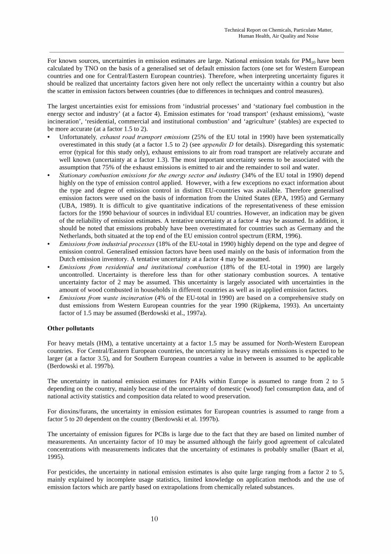
For known sources, uncertainties in emission estimates are large. National emission totals for PM10 have beencalculated by TNO on the basis of a generalised set of default emission factors (one set for Western Europeancountries and one for Central/Eastern European countries). Therefore, when interpreting uncertainty figures itshould be realized that uncertainty factors given here not only reflect the uncertainty within a country but alsothe scatter in emission factors between countries (due to differences in techniques and control measures).
The largest uncertainties exist for emissions from ‘industrial processes’ and ‘stationary fuel combustion in theenergy sector and industry’ (at a factor 4). Emission estimates for ‘road transport’ (exhaust emissions), ‘wasteincineration’, ‘residential, commercial and institutional combustion’ and ‘agriculture’ (stables) are expected tobe more accurate (at a factor 1.5 to 2).• Unfortunately��H[KDXVW�URDG� WUDQVSRUW�HPLVVLRQV (25% of the EU total in 1990) have been systematically
overestimated in this study (at a factor 1.5 to 2) (see DSSHQGL[�' for details). Disregarding this systematicerror (typical for this study only), exhaust emissions to air from road transport are relatively accurate andwell known (uncertainty at a factor 1.3). The most important uncertainty seems to be associated with theassumption that 75% of the exhaust emissions is emitted to air and the remainder to soil and water.
• 6WDWLRQDU\�FRPEXVWLRQ�HPLVVLRQV�IRU�WKH�HQHUJ\�VHFWRU�DQG�LQGXVWU\ (34% of the EU total in 1990) dependhighly on the type of emission control applied. However, with a few exceptions no exact information aboutthe type and degree of emission control in distinct EU-countries was available. Therefore generalisedemission factors were used on the basis of information from the United States (EPA, 1995) and Germany(UBA, 1989). It is difficult to give quantitative indications of the representativeness of these emissionfactors for the 1990 behaviour of sources in individual EU countries. However, an indication may be givenof the reliability of emission estimates. A tentative uncertainty at a factor 4 may be assumed. In addition, itshould be noted that emissions probably have been overestimated for countries such as Germany and theNetherlands, both situated at the top end of the EU emission control spectrum (ERM, 1996).
• (PLVVLRQV�IURP�LQGXVWULDO�SURFHVVHV (18% of the EU-total in 1990) highly depend on the type and degree ofemission control. Generalised emission factors have been used mainly on the basis of information from theDutch emission inventory. A tentative uncertainty at a factor 4 may be assumed.
• (PLVVLRQV� IURP� UHVLGHQWLDO� DQG� LQVWLWXWLRQDO� FRPEXVWLRQ (18% of the EU-total in 1990) are largelyuncontrolled. Uncertainty is therefore less than for other stationary combustion sources. A tentativeuncertainty factor of 2 may be assumed. This uncertainty is largely associated with uncertainties in theamount of wood combusted in households in different countries as well as in applied emission factors.
• (PLVVLRQV� IURP�ZDVWH� LQFLQHUDWLRQ (4% of the EU-total in 1990) are based on a comprehensive study ondust emissions from Western European countries for the year 1990 (Rijpkema, 1993). An uncertaintyfactor of 1.5 may be assumed (Berdowski et al., 1997a).
2WKHU�SROOXWDQWV
For heavy metals (HM), a tentative uncertainty at a factor 1.5 may be assumed for North-Western Europeancountries. For Central/Eastern European countries, the uncertainty in heavy metals emissions is expected to belarger (at a factor 3.5), and for Southern European countries a value in between is assumed to be applicable(Berdowski et al. 1997b).
The uncertainty in national emission estimates for PAHs within Europe is assumed to range from 2 to 5depending on the country, mainly because of the uncertainty of domestic (wood) fuel consumption data, and ofnational activity statistics and composition data related to wood preservation.
For dioxins/furans, the uncertainty in emission estimates for European countries is assumed to range from afactor 5 to 20 dependent on the country (Berdowski et al. 1997b).
The uncertainty of emission figures for PCBs is large due to the fact that they are based on limited number ofmeasurements. An uncertainty factor of 10 may be assumed although the fairly good agreement of calculatedconcentrations with measurements indicates that the uncertainty of estimates is probably smaller (Baart et al,1995).
For pesticides, the uncertainty in national emission estimates is also quite large ranging from a factor 2 to 5,mainly explained by incomplete usage statistics, limited knowledge on application methods and the use ofemission factors which are partly based on extrapolations from chemically related substances.
Technical Report on Chemicals, Particulate Matter, Human Health, Air Quality and Noise
�������� 0HWKRGRORJ\�IRU�FDOFXODWLQJ�WUDQVSRUW�DQG�GHSRVLWLRQThe general concept of the atmospheric transport models EUTREND and EUROS centres on the concentrationof substances in air being calculated from its emissions and subsequently transported by the mean wind flow anddispersed by atmospheric turbulence. Meanwhile, the substance is removed from the atmosphere by dry and wetdeposition and (photo-)chemical degradation.
(875(1'
Heavy metals, dioxins/furans, B(a)P and atrazine were calculated with the EUTREND model (Van Jaarsveld,1995), used in many studies on the deposition of contaminants over Europe and the seas forming its borders(Warmenhoven et al., 1989; Van den Hout et al., 1994; Van Jaarsveld et al., 1997). Recently, the EUTRENDmodel has been used for the calculation of the depositions of heavy metals to the convention waters in theframework of OSPARCOM (Van Pul et al., 1998). The model also participated in the model intercomparisonstudy carried out by EMEP/MSC-E (Sofiev et al., 1996).
In the model the dispersion and advection at a long range are described using trajectories assuming a well-mixedboundary layer, while local transport and dispersion is described with a Gaussian plume model. The latter describesthe air concentration as a function of source height and meteorology-related dispersion parameters but, in the caseof high stacks, it also allows for (temporary) transport of pollutants above the well-mixed boundary layer.
Transport and deposition of particles is calculated separately by the model for five different size-classes separately,each with specific deposition parameters. Particle growth is not incorporated in the model but is implicitly assumedto take place in the lowest size-class (d < 10m). The particle size distribution which has to be specified is thedistribution of the particles as they are primarily emitted. As the larger particles tend to be removed faster thansmall particles, the actual size distribution is a function of transport distance and hence also of the effectivedeposition velocity. Size distributions used in this study, based on measured values in the Netherlands, are takenfrom Van Jaarsveld et al. (1986).
The deposition velocity is also a function of the roughness of the receptor area. The deposition velocity abovegrass, which is the dominant land cover, is taken for use in the EUTREND model domain. However, thedeposition velocity above forests is considerably larger i.e. typically a factor of 2 to 3 (Ruijgrok et al., 1994)�Therefore adjustments using a factor 2 and 3 of the deposition to forests were made to the original calculationsof the deposition.
(8526
The pesticides endosulfan, lindane and PCP were calculated with the EUROS model. EUROS is an Eulerianatmospheric transport model which describes the advection and dispersion of substances in the lowertroposphere. This model has been used for acidification and ozone calculations (De Leeuw and Van RheineckLeyssius, 1990; Van Loon, 1996) and has recently been extended to describe the deposition of persistent organicpollutants (POP) as well (Jacobs and Van Pul, 1996). Part of this model development is carried out incoöperation with MSC-E of the UN-ECE/EMEP framework.
Since many POP are semi-volatile at atmospheric conditions they may be re-emitted from the soil and watersurfaces where they have been deposited. Due to the deposition and re-emission cycling of POP, the descriptionof the deposition process generally used for components which only deposit, such as most acidifyingcomponents and heavy metals, cannot be applied. Instead, deposition should be considered as a net deposition,i.e. the sum of the deposition and re-emission fluxes. For this reason, a dynamic model which describes thegaseous exchange of POP at soil and sea surfaces (dry-deposition and re-emission) was coupled to the EUROSmodel (Jacobs and Van Pul, 1996).
Technical Report on Chemicals, Particulate Matter, Human Health, Air Quality and Noise
The uncertainties in modelling depositions of HMs and POPs are very large, particularly for POPs. The totaluncertainty in the deposition calculations is caused by:a) uncertainties introduced by the model concept,b) uncertainties in substance-specific parameters,c) uncertainties in emissions.
Ad a) This includes all the processes relevant in describing dispersion and deposition. Such general aspects canbe tested using the model for substances such as SO2, for which much more reliable data (emissions andmeasurements) are available. This type of uncertainty is expected to be relatively small (in the order of ± 30%for the deposition on a yearly basis). The range in the deposition data due to different meteorological conditionsis also included in this figure.
Ad b) The choice of deposition parameters has a great impact on the calculated deposition. The dry and wetdeposition rates of the HM are highly dependent on the particle size. The uncertainty of the particle sizedistribution of the emitted compounds could cause a range in the deposition of 30-50%.For POP, the dry and wet deposition rates are also dependent on the physicochemical properties of the substanceand properties of the receiving surface. The uncertainty in the yearly deposition data is estimated at a typicalfactor of 2.
Ad c) The uncertainties in the emissions are large as has been discussed in VHFWLRQ���������
A comparison between calculated and measured heavy metal concentrations in air (EMEP/CCC andOSPAR/CAMP networks) showed, in general, a good correlation (R2 = 0.6-0.7) close to the 1:1 line. Practicallyall calculated depositions are within a factor of 2 of the measurements. However, for Cd and Pb two distinctregions in concentration levels are found: lower values in NW Europe (coastal stations) and higher values inCentral Europe. For Cd, this means that the calculations underestimate the measurements by a factor of 2. Thiswas also found in the study on deposition to the Convention Waters of OSPARCOM (Van Pul et al., 1998).
PAH and dioxins/furans do not form part of any monitoring programme in Europe. Therefore very limitedmeasurement data (mostly urban and data for campaigns) are available to check the model results on a Europeanscale. Van Jaarsveld and Schutter (1993) and Van Jaarsveld et al. (1997) have carried out a validation of theirEUTREND model calculations for B(a)P and dioxins using soil data and some national monitoring data. Theyconcluded that the agreement between modelled and calculated levels, in general, was fairly good. For B(a)Pconcentrations were found to be underpredicted in remote areas and overpredicted in industrial areas. Since thesame model is used in this study, deviations from the above findings will be mainly due to a difference inemission data.Of the pesticides only for lindane are a few measurements available from the EMEP/OSPAR network (Nordiccountries and locations round the North Sea). This comparison between model calculations and methods showedcalculations to approximately overestimate the measurements by a factor of 3. For endosulfan and PCP no datacould be found. Since both substances have similar physicochemical properties to lindane, it is expected that theuncertainty in the results will be in the same order of magnitude as for lindane, i.e. where the uncertainty in theemissions is not taken into account. Previous calculations for atrazine showed the EUTREND modelledconcentrations to be seemingly in reasonable agreement with measured data (within a factor of 2 of 3) in theNetherlands and Northern Germany (Baart et al, 1995).
Technical Report on Chemicals, Particulate Matter, Human Health, Air Quality and Noise
�������� 0HWKRGRORJ\�IRU�FDOFXODWLQJ�FULWLFDO�ORDGVThe critical loads for cadmium, lead and copper were calculated with both a steady-state and simple dynamicapproach as described in detail by De Vries and Bakker (1998). Critical loads are computed on the basis ofeither:• critical dissolved metal concentrations, since these criteria are good indicators of ecotoxicological effects.
Using this steady-state approach implies that adsorption and complexation descriptions are not needed, andthat critical load is mainly dependent on hydrological and vegetation data.
• a simple dynamic approach in which the accumulation up to a given critical metal content in the soil isaccepted in a finite period (100 years) as preferred to an infinite period (steady-state approach). Thisapproach, which implies the use of metal content present, may be regarded as one of the methods to derivetarget loads.
At the Bad Harzburg workshop it was recommended to calculate the target loads using the simple dynamicapproach for a time frame of 50-100 years and the steady-state critical loads for infinity.In this study all critical load maps were calculated with the simple dynamic approach using a time frame of 100years.
�������� 8QFHUWDLQWLHV�LQ�FULWLFDO�ORDGVVarious sources of uncertainty in deriving critical loads exist, namely critical limits, calculation methods andinput data. Uncertainties due to differences in critical limits can be very large. Uncertainties in calculationmethods due to assumptions, such as equilibrium partitioning in a homogeneously mixed system, may give riseto a high uncertainty in certain situations. The uncertainty in data, either by spatial variability or because of lackof knowledge, can be quantified through an uncertainty analysis. Such an analysis, which also gives insight intowhich parameters are main determinants of the uncertainty in the resulting critical load, has been performed forcadmium and copper (Groenenberg 1999, in prep.). This uncertainty analysis was carried out for critical loadscalculated with (i) a steady-state model, using background concentrations in the soil solid phase as critical limitsand (ii) a simple dynamic model, using effect-based critical concentrations in the soil solution, including anacceptable net accumulation in the soil. Results showed that parameters describing the adsorption are generallyof importance for both cadmium and copper, and both types of models and critical limits. Additionally,complexation plays a dominant role for copper, whereas hydrological parameters are important for cadmium,especially when using a dynamic model combined with a critical limit for the soil solution.
Technical Report on Chemicals, Particulate Matter, Human Health, Air Quality and Noise
The primary objectives of the emission calculations performed are:• to assess future trends in emissions of primary PM10
4 and selected HMs and POPs based on existing EU andECE policies, and to compare these baseline trends with emission targets insofar as such targets have beenset,
• to assess spill-over effects of policy action in the field of climate change (Kyoto targets) and acidification(proposed EU National Emission Ceilings directive),
• to address further policy measures for emissions control of primary PM10 and selected HMs and POPs.
Three principal emission scenarios have been assessed in this study (VHH�%R[����). Making use of a 1990-2010timeframe, future trends in emissions under current legislation were assessed in the baseline scenario (BL),while the technology-driven scenario (TD) assumes full penetration of advanced end-of-pipe emission controltechnologies, such as high efficiency electrostatic precipitators, fabric filters and highly efficient wet scrubbers.The accelerated policy scenario (AP) takes into account the effects of accelerated policy action on climatechange (Kyoto targets) and acidification (proposal for NEC-directive). Advanced end-of-pipe technologies toreduce emissions of PM10 and selected HMs and POPs are considered in the AP-scenario also5. Assessedcontrol options are presented in detail LQ�VHFWLRQ��������.
Calculations have been performed at the country level. A description of projected baseline changes to basicsocio-economic parameters such as population, GDP growth and energy consumption is presented LQ�7HFKQLFDO5HSRUW�6RFLR�(FRQRPLF�7UHQGV��0DFUR�(FRQRPLF� ,PSDFWV�DQG�&RVW� ,QWHUIDFH. The scenarios BL and TD arebased on the ‘pre-Kyoto Business-as-Usual’ energy scenario (BAU). The AP-scenario is based on the ‘post-Kyoto no-trade’ energy scenario. For this ‘post-Kyoto no-trade’ energy scenario it was assumed that theprovisions of the Kyoto protocol are met assuming no-trade in GHG emissions. Details incl. costs concerningassumed control measures for the attainment of Kyoto protocol targets and NEC-targets are evaluated in thecontext of the technical reports on Acidification, Eutrophication and Tropospheric Ozone and Climate Changerespectively.
The ‘post-Kyoto no-trade’ energy scenario differs substantially from the BAU-scenario. Total primary energysupply for the ‘post-Kyoto no-trade’ energy scenario is about 10% decreased when compared to BAU (6700PJ); consumption of coal and oil (for energy purposes) falls by 46% (3100 PJ) and 16% (4200 PJ), respectively,and consumption of gas (for energy purposes) is more or less unchanged. The use of other fuels such as wasteand biomass rises about 30% (700 PJ).
Under the AP-scenario, spill-over effects from policy action on climate change and acidification were analysedseparately from the effects of full application of advanced abatement technologies for control of PM10 andselected HMs and POPs. Results of the spill-over calculations are presented as separate scenarios in thisbackground report (see box). The Spill-Over Kyoto Protocol scenario (SO-KP) considers spill-over effects ofKyoto protocol targets only. The Spill-Over scenario (SO) considers effects of Kyoto Protocol targets as well asproposed national emission targets for acidification specified in the proposal for the EU-National EmissionCeilings directive.
4 Particles with diameter less than 10 µm (<0.01 mm) that can follow the inhaled air into the respiratory systemand the lungs5 For the macro-economic feedback only costs involved with PM emission control have been taken into account.
Technical Report on Chemicals, Particulate Matter, Human Health, Air Quality and Noise
Control measures included in the various scenarios will be overviewed here.
Hazardous chemicals are largely emitted in solid form adsorbed onto particles and thus may be effectivelycontrolled by dust arresters such as electrostatic filters, fabric filters and scrubbers. This applies to most heavymetals. However, a substantial amount of mercury is emitted in the vapour phase, just like organic pollutantssuch as dioxins/furans and PAHs. To minimize the emissions of these partly gaseous pollutants, specialtechniques should be installed in addition to dust arresters.
Dust emissions may be reduced by improved operation of the combustion or production process, or by cleaningof the flue gas. Cleaning of exhaust gases by some type of dust arrester is common practice in coal combustionin power plants and industry, and also in many industrial production processes. Oil-fired installations in powerplants and industry are, in general, not equipped with any dust cleaning device as is the case for firing devices inthe ‘residential, commercial and institutional’ sector and motor engines. Dust emissions by municipal wasteincineration are generally effectively controlled within the EU, although in some EU countries6 significantamounts of municipal waste are incinerated without an any type of emission control (Berdowski et al., 1997a,d).However, the situation in these countries is improving thanks to current EU legislation.
It should be noted that measures to reduce emissions of acidifying compounds, such as desulfurization processesand low-S fuels, also have substantial side-effects on emissions of particulates and adsorbed chemicals.
6 France, Italy, Spain, United Kingdom
Box 1.2.: Emission scenarios
The Baseline scenario (BL) is based on the Business-As-Usual socio-economic scenario presented inTechnical report on Socio Ecnonomic Trends, Macro Economic Impacts and Cost Interface, assuming thecontinued implementation of existing EU policies as of August 1997. All measures or policies agreed uponafter that date are not included in the Baseline scenario. Furthermore, spill-over effects resulting from thecontinued post-1990 implementation of current policies in the field of acidification have not been consideredin this scenario.
The Technology Driven scenario (TD) assesses maximum feasible emission reductions in the year 2010,assuming full application of advanced end-of-pipe emission control technologies for particulates, HMs andPOPs, against the background of the BAU-scenario.
The Spill-Over Kyoto Protocol scenario (SO-KP) has been developed to assess the spill-over effects ofpolicy action on climate change i.e. Kyoto Protocol targets, assuming no trade in GHG emissions. Spill-overeffects have been assessed by repeating BL-calculations using a ‘post-Kyoto no-trade’ energy scenario,keeping all other socio-economic parameters unchanged.
In addition, a Spill-Over scenario (SO) has been developed to assess spill-over effects of policy action onclimate change as well as on acidification. This scenario incorporates Kyoto Protocol targets and proposedEU national emission targets for acidification. In addition, this scenario incorporates new EURO-4particulates emission standards for motor vehicles to be introduced from 2005, as accepted by the Counciland the European Parliament in 1998.
Finally, an Accelerated Policy scenario (AP) has been developed to assess maximum feasible emissionreductions in 2010, assuming Kyoto targets are met, and also full application in 2010 of advanced emissioncontrol technologies for particulates and selected HMs and POPs. The AP scenario assumes an unrealisticrapid turnover rate for technologies: for example, the complete motor vehicle fleet has been assumed tocomply with EURO-4 emission standardsin 2010.
Technical Report on Chemicals, Particulate Matter, Human Health, Air Quality and Noise
%/��VWDWLRQDU\�VRXUFHV• Large Combustion Plants Directive (EC, 1988, 88/609/EEC); emission limits are 50 mg/Nm3 for dust for
new (post-1987) combustion plants > 500 MWth and 100 mg/Nm3 for new combustion plants between 50and 100 MWth. The majority of utility and industrial combustion plants in the EU already complied with these dustemission limit values in 19907 (Berdowski et al., 1998). Thus, there is no legal obligation to reduce dustemissions further. Nevertheless, it may be expected that dust emissions from large combustion installationswill decline substantially in the period 1990 to 2010 due to spill-over effects of SO2-related controlmeasures (SO2 emission standards). Such spill-over effects are not included in the baseline scenario.
• Municipal Waste Incineration directives for existing installations (EC, 1989b, 89/429/EEC) and for newinstallations (EC, 1989a, 89/369/EEC): general emission limit values of 30 mg/Nm3 for dust and 0.2mg/Nm3 for mercury have been applied. For dioxins/furans a limit value of 0.1 ng I-Teq/Nm3 has been usedin line with the Commission proposal for the amendment of current waste incineration directives8 (EC,1999a).
• Decreases in S-content of heavy fuel oil in oil refineries: a 40% reduction in the 1990 emission factor hasbeen assumed (Visschedijk et al., 1998).
%/��PRELOH�VRXUFHV• Compliance with EURO-3 particulates emission standards (phase-in from 2000) has been assumed for
passenger cars, light-duty vehicle and heavy-duty vehicles. A lifetime of 10 years has been assumed for allvehicles.
7HFKQRORJ\�'ULYHQ�VFHQDULR��7'� 7'��VWDWLRQDU\�VRXUFHV• High performance 4-field electrostatic precipitators have been assumed for coal and biomass combustion in
the ‘Public power, cogeneration and district heating’ and ‘Industrial combustion’ sectors, with an assumedparticle concentration in the flue gas of 20 mg/m3 (Visschedijk et al., 1998).
• Electrostatic precipitators have been assumed for heavy fuel oil combustion in the ‘Public power,cogeneration and district heating’ and ‘Industrial combustion’ sectors.
• Combustion systems with optimised burning rates have been assumed for coal and biomass combustion inthe ‘Residential, Commercial and Institutional combustion’ sector, with an assumed overall abatamentefficiency of 25% (UN/ECE, 1998b; Hulskotte et al., 1999).
• For reducing dust emissions from industrial processes9, many different control measures such as highperformance electrostatic precipitators, fabric filters, and highly efficient wet scrubbers combined withwaste gas collection systems have been assumed. In addition, specially designed techniques have beenassumed for the control of gaseous emissions (Visschedijk et al., 1998; Berdowski et al., 1997c; 1998).
• For municipal waste incineration, emission standards have been assumed to be in line with the proposal forthe amendment of current EU waste incineration directives: emission limit value of 10 mg/Nm3 for dust 10 ,0.05 mg/Nm3 for mercury and 0.1 ng I-Teq/Nm3 for dioxins/furans (EC, 1999a).
• A full switch to PAH-free techniques for wood preservation has been assumed.
7 With the exception of ‘industrial combustion’ and ‘industrial processes’ in southern Europe (Spain, Greece,Italy and Portugal) which in 1990 did not fully comply with requirements of the Large Combustion PlantDirective for dust.8 Strictly speaking, the emission limit value for dioxins/furans of 0.1 ng I-Teq/Nm3 should not be accounted forin the Baseline because this standard had not yet been decided on by the EU per August 1997.9 Non-combustion related emission sources in ferrous, non-ferrous, cement, glass, chloro-alkali and the oilrefining industry.10 TD-scenarios for waste incineration are by mistake based on a dust standard of 30 mg/Nm3 (=BL-value)although the stricter TD-value of 10 mg/Nm3 should have been used. However, effects on presented results arenegligible.
Technical Report on Chemicals, Particulate Matter, Human Health, Air Quality and Noise
7'��PRELOH�VRXUFHV• Compliance with EURO-4 particulates emission standards (phase-in from 2005) has been assumed for
passenger cars, light-duty and heavy-duty vehicles• Particulates emission standards in compliance with EURO-2 for heavy duty vehicles have been applied for
vehicles in the off-road transport sector. 6SLOO�RYHU�.\RWR�3URWRFRO�VFHQDULR���62�.3�
In addition to control measures listed for the BL scenario, the SO-KP scenario incorporates spill-over effectsfrom policy action on climate change i.e.:• Kyoto targets for reduction of GHG emissions, assuming no trade in emissions. 6SLOO�RYHU�VFHQDULR��62� In addition to spill-over effects from climate change, the SO-scenario incorporates spill-over effects fromacidification (proposed EU National Emission Ceilings Directive) i.e.:• Limit sulfur content in heavy fuel oil to 1% (EC, 1999b).• Spill-over effects are caused by the continued (post-1990) penetration of flue gas desulfurization techniques
(FGD) on coal combustion in the ‘Public power, cogeneration and district heating’ and ‘Industrialcombustion’ sectors. Spill-over effects have been calculated on the basis of IIASA estimates for thepenetration of FGD technology in the separate EU countries in the years 1990 and 2010 (VHH�7HFKQLFDO5HSRUW�RQ�$FLGLILFDWLRQ��(XWURSKLFDWLRQ�DQG�7URSRVSKHULF�2]RQH��(&������); with particle concentrationlevels in the exhaust gas -without and with FGD - of resp. 50 and 20 mg/Nm3 (EEA/EMEP, 1996).
• A realistic turnover rate of 10 years has been modelled for passenger cars, light-duty and heavy-dutyvehicles. Thus, half the vehicle fleet is anticipated to satisfy EURO-4 emission standards (phase-in from2005) in 2010; the other half is anticipated to comply with the less stringent EURO-3 standards (phase-infrom 2000).
• Particulates emission standards complying with EURO-2 for heavy duty vehicles have been applied forvehicles in off-road transport sector.
Spill-over effects caused by by an EU limit of 0.1% for the sulphur content of gasoil for stationary sources(directive on sulfur in liquid fuels) is not reflected in the AP-NT scenario, because of a lack of information onthe relationship between S-percentage for gasoil and particulates emissions. However, these effects, based onpreliminary calculations using available relationships for heavy fuel oil, are expected to be rather small.
$FFHOHUDWHG�3ROLF\�VFHQDULR��$3�
The AP scenario projects emissions, taking into account the effects of policy action on climate change andacidification. High performance technologies to reduce emissions are considered also (see list of controlmeasures mentioned above for the TD-scenario).
Technical Report on Chemicals, Particulate Matter, Human Health, Air Quality and Noise
This section on emissions and costs starts with a brief general analysis of the formation and emissions to air ofprimary PM10 and selected HMs and POPs. Next, main anthropogenioc source sectors in 1990 are assessed.Finally, results for the calculated emission scenarios are discussed.
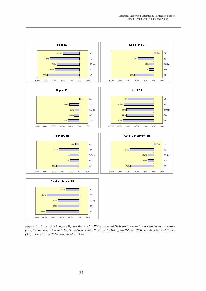
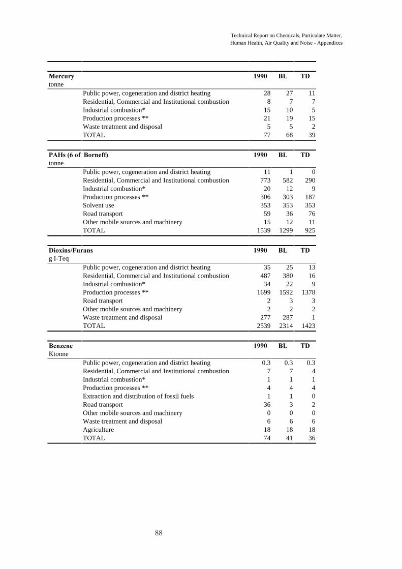
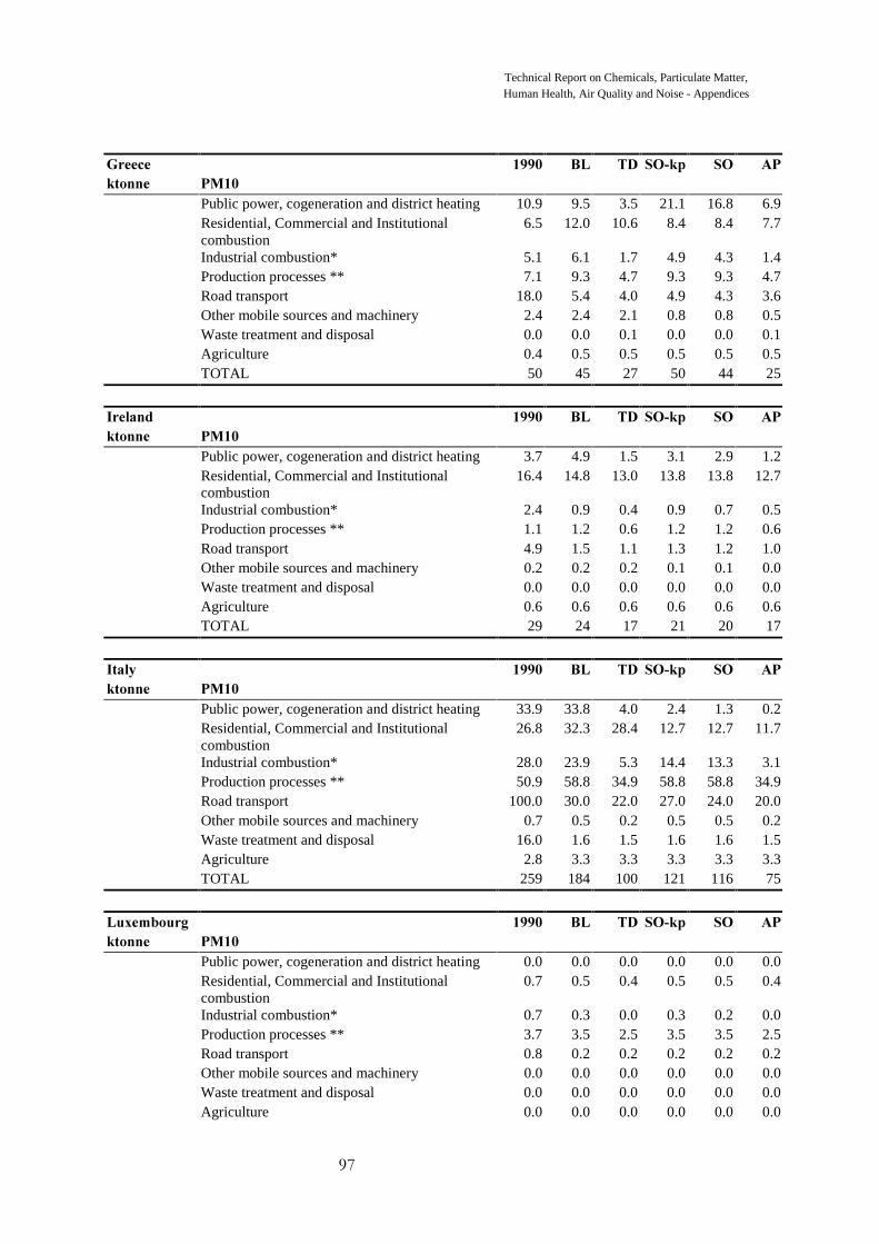
Emission tables for the base year 1990 and different scenarios are presented for the EU-region in $SSHQGL[�$��.For PM10, emissions are also presented by country (VHH�$SSHQGL[�%��). )LJXUH����� illustrates the differencesbetween scenarios for the EU-region in terms of percentage emission reduction in 2010 compared to 1990. Afurther analysis of results is presented in ILJXUHV������WR����� (contribution of sectors in EU-totals in 1990 and in2010, relevance of various source categories for overall EU-emission trends 1990-2010, percentage change inemissions by sector 1990-2010)
2ULJLQ�RI�HPLVVLRQV
Heavy metals are present in trace amounts as a natural element of fossil fuels and biomass, and raw materialssuch as iron, zinc, copper and lead ores. Consequently, combustion and industrial processes are, in principle,important potential emitters of heavy metals. Furthermore, metals are used in a variety of products such aspigments, batteries, fuel additives and fertilisers. These products end up in the waste stream and may ultimatelybe disposed of by incineration, giving rise to air emissions. Emission rates of heavy metals are determined bythe content of trace elements in the fuels or wastes combusted or the raw materials processed, by the appliedcombustion or production technology, and by the efficiency of the emission control equipment (dust abatementand specific techniques for capturing gaseous heavy metals).
The heavy metal content (expressed in terms of energy content of the fuel) for lead, copper and mercury is onaverage one order of magnitude higher in coal than in oil. Cadmium content of coal and oil are more comparable(EEA/EMEP, 1996). Heavy metal content of natural gas is negligible.
Dioxins/furans are emitted from thermal processes involving organic material and chlorine-containingsubstances as a result of incomplete combustion or chemical reactions. Dioxins/furans are emitted for the largerpart in the vapour phase, but also partly adsorbed onto dust particles. Approximately 80% of dioxins/furans isemitted in the gaseous phase at temperatures above 300 oC, while 90% is adsorbed onto dust particles attemperatues below 70%.
Emissions of PAHs are the result of incomplete combustion of fossil fuels, waste materials and other fuels suchas biomass, and the use of PAH-containing coal-tar products for wood preservation.
(8��EDVH�\HDU�����
Source categories used for this study are consistent with level 1 of the UN/ECE-source category classification(SNAP90; EEA, 1995; EEA/EMEP, 1996). Only the treatment of refineries is different from SNAP90; i.e.emissions for refineries have been fully accounted for in SNAP-sector 4 ‘production processes’. The followingsource categories have been distinguished in this study (with corresponding SNAP90 codes in parentheses anddeviations from SNAP90 in italics):• Public power, cogeneration and district heating (01)• Residential, Commercial and Institutional (RCO) combustion (02)• Industrial combustion �H[FO��FRPEXVWLRQ�LQ�SHWUROHXP�LQGXVWULHV�� (03)• Production processes (LQFO��FRPEXVWLRQ�LQ�SHWUROHXP�LQGXVWULHV�� (04)• Extraction and distribution of fossil fuels (05)• Solvent use (06)• Road transport (07)• Other mobile sources and machinery (08)• Waste treatment and disposal (09)• Agriculture (10)
Technical Report on Chemicals, Particulate Matter, Human Health, Air Quality and Noise
The contribution of various UN/ECE-source categories to total EU emissions in 1990 is illustrated in ILJXUH�����and will be briefly discussed below for the various compounds.
• 3DUWLFXODWH�PDWWHU������µP�PM10 emissions in EU countries are caused by different source categories, the most important sectors beingcombustion in the energy and industrial sectors (SNAP1/3 − 34% of EU-total), combustion in road transport(24%), combustion in households and services (SNAP2 − 18%) and industrial production processes (SNAP4−18%).
Emissions from combustion in stationary sources is mainly due to coal (70%). Oil and other fuels (such asbiomass) contribute 19% and 10%, respectively.
Emissions from industrial production processes are mainly due to the ferro and non-ferro industry (43%) and oilrefineries (43%).
In interpreting the PM10 results of this study, it should be realised that available information on non-exhaustemissions by road transport is very scarce. The magnitude of non-exhaust PM10 emissions in this study formsonly 5% of total road transport emissions (see $SSHQGL[�'). Non-exhaust is specified here as tyre, brake androad wear. Some information is available for these sources, although very scarce. However, in this study, noaccount is taken of resuspension of dust due to the motion of vehicles along the road.
• &DGPLXPCadmium emissions in the EU are mainly (38%) due to industrial production processes (40%); other significantsources are combustion in the energy sector and industry (25%) and road transport (19%); minor sources arewaste incineration (8%) and combustion in households and services (5%).
Emissions by combustion in stationary sources are caused by the combustion of oil (42%), coal (35%) and otherfuels, such as biomass (23%). The relative high contribution of oil to total emissions compared to other heavymetals is caused by the relative high cadmium emission factors for oil combustion.
Emissions by industrial production processes are almost completely (95%) due to the ferrous and non-ferrousmetal industry.
• &RSSHUAbout half the�copper emissions come from mobile sources (48%) i.e. road transport (26%) and other transport(22%); other significant sources are combustion in the energy sector and industry (25%) and industrialproduction processes (26%).
Emissions from stationary combustion sources are mainly due to combustion of coal (68%). Oil and other fuels(such as biomass) contribute 17% and 15%, respectively.
Emissions from industrial production processes are almost entirely caused by the ferrous and non-ferrous metalproduction industry (98%).
• /HDGLead emissions are largely (80%) caused by road transport i.e. lead in gasoline; industrial processes representthe other significant source (12%).
Emissions by industrial production processes are almost entirely caused by the ferrous and non-ferrous metalindustry (90%).
• 0HUFXU\Mercury emissions are mainly caused by industrial production processes in the non-ferrous metal (17%), cement(15%), chloro-alkali (11%) and iron and steel industries (3%). Other significant sources are combustion in theenergy sector and industry (32%), and waste incineration (17%).
Technical Report on Chemicals, Particulate Matter, Human Health, Air Quality and Noise
Emissions from stationary combustion sources are mainly due to combustion of coal (66%). Other fuels (such asbiomass) and oil contribute 30% and 4%, respectively.
• 'LR[LQV�)XUDQVEmissions of dioxins and furans (PCDD/Fs) are mainly caused by the waste incineration sector (41%). Othersources are combustion in the energy sector and industry (26%), industrial production processes (21%) andcombustion in households and services (10%).
Emissions by stationary combustion sources are largely caused by the combustion of other fuels (such asbiomass) (45%) and coal (38%). Emissions from oil are less important (17 %).
Emissions by industrial production processes arise mainly from the iron and steel industry (76%), non-ferroindustry (12%) and other industrial processes (11%).
• 3RO\F\FOLF�$URPDWLF�+\GURFDUERQV��3$+V�Emissions of Polycyclic Aromatic Hydrocarbons (Borneff 6 PAHs) are due to solvent use (39%), combustion inhouseholds and services (26%), road transport (19%) and industrial production processes (12%).
Emissions due to solvent use are determined primarily by wood preservation with PAH-containing coal-tarproducts. Emissions may occur during the impregnation process as well as during storage, handling and use ofthe impregnated wood. The most widely used coal-tar products are carbolineum and creosote.
Emissions from stationary combustion sources are primarily caused by the combustion of other fuels such aswood (62%) and coal (37%). Emissions from oil are negligible (1%). Furthermore, emissions from stationarycombustion are mainly caused by combustion in households (84%). This is the result of using small firinginstallations in households that are less optimized than installations used in the energy sector and industry; thisleads to more incomplete combustion and thus higher PAH emissions.
About half the emissions from industrial production processes are caused by non-ferrous metals production(52%), mainly in the aluminium industry. Other major industrial sources are the iron and steel industry (23%),primarily coke production, and asphalt road paving companies (26%).
• 3RO\FKORULQDWHGELSKHQ\OV��3&%V�Emissions of Polychlorinatedbiphenyls (PCBs)�are mainly (about 80%) caused by the leaks and spills fromclosed electrical equipment such as transformers and capacitors. The other major source is re-emission fromcontaminated water and soil. The formation of PCBs in high temperature processes (stationary combustion andwaste incineration) is relative unimportant in the baseyear 1990.
• 3HVWLFLGHVPesticides atrazine and endosulfan are mainly used in the agricultural sector. Pentachlorophenol and lindane arealso used by industry for various applications.
�������� (8��%DVHOLQH�VFHQDULR�IRU�������%/�
6FRSHThe Baseline scenario (BL) assesses future trends in emissions under current legislation. The BL is based on thebusiness-as-usual socio-economic scenario (VHH� 7HFKQLFDO� 5HSRUW� 6RFLR� (FRQRPLF� 7UHQGV�� 0DFUR� (FRQRPLF,PSDFWV� DQG�&RVW� ,QWHUIDFH); assuming the continued implementation of existing and proposed EU and ECEpolicies as of August 1997. All measures or policies agreed upon after that date are not accounted for in theBaseline.
Emission targets have been established for selected heavy metals (HM) and persistent organic pollutants (POP)in the framework of the United Nations Convention on Long Range Transboundary Air Pollution). According tothe UN/ECE-protocols on HM and POP (UNECE, 1998a,b) countries are obliged to reduce atmosphericemissions of lead, cadmium, mercury, dioxins/furans and polycyclic aromatic hydrocarbons below the levels ina reference year, most probably 1990 for the EU.
Technical Report on Chemicals, Particulate Matter, Human Health, Air Quality and Noise
The BL presented does not incorporate spill-over effects from the continued post-199011 penetration of controloptions in the field of acidification, such as flue gas desulfurization (FGD) techniques on coal boilers in theenergy sector and industry (effecting emissions of PM10, HM, POP) and the reduction of the sulfur content inheavy fuel oil to 1% (effecting PM10). Furthermore, the BL only reflects current emission standards laid down inEU directives and ECE protocols12; more stringent QDWLRQDO policies for emissions control of particulates, HMsand POPs are not accounted for. This methodology was decided on because detailed national data on a sectorbasis were not always available. The sectors ‘power generation’, ‘industrial combustion’, ‘industrial processes’and ‘residential, commercial and institutional combustion’ are estimated to have already complied with currentinternational standards in the base year 1990 (Berdowski et al., 1998). Consequently, no future improvement inthe emission has been modelled for these categories under the BL. For other major sectors, i.e. ‘road transport’and ‘waste incineration’, 1990 compliance with EU/ECE standards was estimated to be incomplete, makingmodelling of future reduction in emission factors under Baseline conditions necessary.
The chosen methodology of unchanged emission factors for stationary combustion sources and industrialprocesses should be considered to possibly lead to an overestimation of future emissions in specific countrieswith an advanced control strategy for particulates and hazardous substances. More stringent national, regional orlocal policies such as permitting requirements and national emission reduction agreements with sectors, maylead to reductions in emissions that go far beyond what may be expected based on EU/ECE requirements only.
$VVHVVPHQW�DQG�WUHQGV
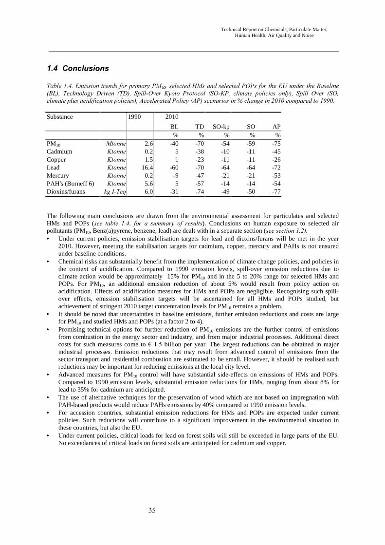
Under current policies, substantial emission reductions are expected by 2010 (compared to 1990) for PM10 (-40%), lead (-60%), dioxins/furans (-31%), and to a lesser degree for mercury (-9%). In addition, emissions ofPCBs, PCP and lindane should be almost negligible in 2010 due to current EU regulations13. With suchreductions, the EU is likely to meet emission stabilisation targets for these HMs and POPs, as established underthe UN ECE CLRTAP Protocols. However, the achievement of emission stabilisation targets for cadmium(+5%), copper (+1%) and PAHs (+5%) is not ensured under baseline conditions14.
The projected downward trend in PM10 emissions results primarily from lower transport emissions andstationary combustion emissions due to stricter emission standards15 and reduced coal use. The phasing out ofleaded gasoline explains the substantial reduction in lead emissions expected in 2010. The marked improvementin emission levels of dioxins/furans is explained by the application of efficient flue-gas cleaning technologies in2010. Reduced coal use and reduced emissions from the chloro-alkali industry, which has adopted an emissionabatement programme for mercury emissions, are expected to bring about lower mercury emissions by 2010.Under the BL, small increases in the emissions of cadmium and PAHs are expected due to growth in roadtransport (for Cd) and higher use of wood fuel in households (for PAHs).
Below, emission changes under current legislation are analysed in more detail in terms of sectoral contributions,and for main sectoral trends in terms of underlying driving forces (i.e. socio-economic developments and controlpolicies). The relevance of various sectors for overall EU-emission trends under baseline conditions is illustratedin )LJXUH����. The change in emissions per sector in the period 1990 to 2010 is presented in )LJXUH����� Thecontribution of various sectors to total EU-emissions is illustrated in )LJXUH����.
• 3DUWLFXODWH�PDWWHU������XP�Emissions of PM10 are expected to decrease substantially by 2010 compared to 1990 (-40%). The downwardtrend is explained by lower emissions from URDG�WUDQVSRUW and VWDWLRQDU\�FRPEXVWLRQ�sources (i.e. combustionin the energy sector and industry, and combustion in the ‘residential, commercial and institutional’ sector).Absolute emission reductions anticipated for both sectors are comparable.
11 Spill-over effects effectuated in the year 1990 are already accounted for in the 1990 emission inventory.12 Possible effects of the general EU-IPPC requirement to use BAT for major industrial activities have not beentaken into account.13 Emissions of atrazine and endosulfan are expected to stabilise.14 Due to new insights, baseline results in this study were revised for PM10, Cd, Hg, Cu, PAHs and thereforediffer from (EEA, 1999, see DSSHQGL[�')15 New post-2005 EURO-4 emission standards for freight and passenger road transport have not been taken intoaccount in the Baseline scenario; these standards were decided upon in 1998 and have been incorporated in theTD- and AP-scenarios.
Technical Report on Chemicals, Particulate Matter, Human Health, Air Quality and Noise
5RDG�WUDQVSRUW emissions are anticipated to decrease by 70% by 2010 compared to 1990, in spite of the highincrease in volume of passenger and freight transport (37% increase in road transport fuel use). This markeddrop in emissions is a result of EU emissions standards for road vehicles being sharpened up�
For VWDWLRQDU\�FRPEXVWLRQ�sourceV an emission reduction of 32% is expected; this is due to an anticipated sharpdecrease in coal use (-40%). A downward trend in coal use is projected for all stationary combustion categoriesi.e. energy sector, industry, and households plus services. The use of natural gas (with almost negligibleemissions) will increase, oil use will more-or-less stabilise. Although the contribution of other fuels (such asbiomass with high emission factors for particulates and also HM and POPs) to total emissions is low, it shouldbe considered that for the sector ‘residential, commercial and institutional combustion’ the effect of reducedcoal use is partly compensated by increased biomass use.
• &DGPLXP Cadmium emissions are anticipated to more or less stabilise in the period 1990 to 2010 (5%). The assessment ofsectoral trends shows that the projected small increase in Cadmium emissions (5%) is explained by a largeincrease in emissions for URDG� WUDQVSRUW that is largely counterbalanced by a decline in emissions for ZDVWHLQFLQHUDWLRQ. Emissions from URDG�WUDQVSRUW are expected to increase by 50% in the 1990-2010 period due tothe increase in the volume of transport. For ZDVWH�LQFLQHUDWLRQ, a decline in the emissions of 83% is projectedwith the introduction of advanced flue-gas cleaning technologies needed for compliance with EU wasteincineration directives. It should be noted that emissions from road transport reported by TNO and used for this study are largelyuncertain. According to the TNO-inventory, the contribution of road transport in total cadmium emissionsgreatly varies from country to country (from 3% for the UK to 65% for Denmark; 19% for the EU). Based onthe UK-inventory, which is well-founded using a survey of cadmium content of various fuels, it can be doubtedwhether road transport really is a major source of cadmium. If UK-results would be extrapolated to all the otherEU-countries road transport would no longer be a major source of cadmium (only 2%). Anticipated emissiontrends for cadmium emissions within the EU under Baseline-conditions would then change from an expectedincrease with 5% to a decrease with about 5%. • &RSSHU Emissions of copper are projected to stabilize by +1% in the 1990 to 2010 period. The assessment of sectoraltrends shows the anticipated large increase in copper emissions from road transport to be counterbalanced by adecline in the emissions from� FRPEXVWLRQ� LQ� WKH� HQHUJ\� VHFWRU� DQG� LQGXVWU\��Road transport emissions areexpected to increase by 52% due to the increase in the volume of transport. Emissions from FRPEXVWLRQ�LQ�WKHHQHUJ\�VHFWRU�DQG�LQGXVWU\ are expected to decrease by 31% due to an anticipated sharp decrease (-40%) in coaluse. • /HDG Emissions of lead will show a sharp decline by 2010 compared to 1990 (-60%) due the phasing out of leadedgasoline. • 0HUFXU\Emissions of mercury are expected to decrease slightly in the 1990 to 2010 period (-9%) due to anticipatedemission reductions for industrial production processes and for combustion emissions in the energy sector andindustry. Emissions for industrial production processes are anticipated to drop by 9% due to a decline in theemissions from the chloro-alkali industry, which has adopted an emission abatement program for mercuryemissions. Emissions for combustion in the energy sector and industry will decline by 18% due to theanticipated decrease in the use of coal.
• 'LR[LQV�)XUDQV Emissions of dioxins/furans are anticipated to show a marked decrease (31%) by 2010 compared to 1990 due toa large decline in emissions in the ZDVWH�LQFLQHUDWLRQ�sector��Emissions from ZDVWH�LQFLQHUDWLRQ are expected todecline by 96% in the 1990-2010 period due to requirements prescribing an emission limit value of 0.1 ng TEQdioxins/furans/Nm3 for municipal waste incineration. Advanced technologies for flue gas cleaning should beinstalled on waste incinerators comprising a combination of dedustment, wet scrubbing and the injection ofactive carbon in the flue gas in an entrained flow reactor followed by a fabric filter. The entrained flow reactoralso serves to remove other gaseous substances such as PAHs and gaseous metals (mainly mercury).
Technical Report on Chemicals, Particulate Matter, Human Health, Air Quality and Noise
• 3RO\F\FOLF�$URPDWLF�+\GURFDUERQV��3$+V�Emissions of PAHs are expected to increase slightly (+5%) in the 1990 to 2010 period. This anticipated smallincrease in emissions is caused by the anticipated large increase in the combustion of other fuels such as wood at44%. The contribution of biomass residential combustion to total PAH emissions is anticipated to increase from15% in 1990 to 28% in 2010.
• 3RO\FKORULQDWHGELSKHQ\OV��3&%V� Production and use of PolychlorinatedBiphenyls (PCBs) in EU countries was already tightly controlled in thebase year, 1990. Remaining emissions in 1990 were mainly due to accidental releases from PCBs used in oldclosed electrical equipment. Current EU regulations on disposal of PCBs ensures that almost all PCBs still inuse in old equipment will be de-contaminated by the year 2010. Therefore, PCB emissions will be almostnegligible in 2010 compared to 1990. Remaining PCB emissions in 2010 will be mainly due to re-emissionfrom contaminated waters and soils, and also due to formation of PCBs in high temperature stationarycombustion processes. • 3HVWLFLGHV Overall pesticide use – measured by mass of active gradient - appears to have been decreasing in most EUcountries over the past two decades (Thyssen, 1999; EEA, 1999). This trend may likely continue in the nearfuture. However, consumption in terms of mass does not necessarily reflect the environmental burden, as moreactive and more specific substances are being developed and penetrate on the market (EEA, 1999). Emissions of four pesticides (pentachlorophenol, lindane, atrazine and endosulfan) have been studied in moredetail in this study. The use of Pentachlorophenol (PCP) has already been strictly controlled by the EU. Unfortunately, emissiontrends for PCP shown in this study do not consider settled EU-directives imposing tight restrictions on the use ofPCP. It is expected that due to these strict regulations emissions of PCP will be largely reduced in 2010. Restrictions on the use of lindane imposed by the UN/ECE-POP-protocol have also not been taken into accountin the Baseline. This was decided upon because the POP-protocol was settled in 1998 and therefore did not fitthe definition of existing EU policies used for this study i.e. policies agreed upon as of August 1997.Nevertheless, it is expected that due to protocol requirements emissions in the EU will be almost negligible in2010. No change in emissions of atrazine and endosulfan is anticipated in the near future.
The 7HFKQRORJ\�'ULYHQ�VFHQDULR��7'� has been developed to assess future emissions assuming full penetrationof advanced end-of-pipe emission control technologies for particulates and hazardous chemicals, such as high-effciency electrostatic precipitators, fabric filters and highly efficient scrubbers. Results of this scenario for theyear 2010 are compared with the Baseline, illustrating the magnitude of the remaining technical potential forfurther emission control. Control strategies causing changes in the structure and levels of energy consumptionand economic activities have been excluded from this scenario. The relevance of various sectors for overallemission trends under TD conditions is illustrated LQ�)LJXUH����.. The change in emissions in the period 1990 to2010 per sector is presented in )LJXUH����� The contribution of various sectors to total EU-emissions isillustrated in )LJXUH�����
The full application of advanced control technologies would significantly reduce emissions of all pollutantsstudied in comparison to baseline results (VHH�)LJXUH������7'�FRPSDUHG�WR�%/). By 2010, 1990 emission levelsof PM10, lead and dioxins/furans would be reduced by about 70% (30-60% for BL); emissions of Hg and PAHswould be approximately 50% (10% for BL) while emissions for cadmium and copper would be reduced by 40%and 25%, respectively (0% for BL). These results clearly demonstrate the substantial technical potentialremaining for the further control of emissions from hazardous substances.
Technical Report on Chemicals, Particulate Matter, Human Health, Air Quality and Noise
Under the AP-scenario, spill-over effects from policy action on climate change and acidification were analysedseparately from the effects of full application of advanced abatement technologies for control of PM10 andselected HMs and POPs. Results of such calculations are presented as separate ‘spill-over’ scenarios (see box).The 6SLOO�2YHU�.\RWR�3URWRFRO��62�.3� scenario considers spill-over effects of Kyoto protocol targets only.The 6SLOO�2YHU��62� scenario�considers effects of Kyoto Protocol targets as well as proposed national emissiontargets for acidification specified in the proposal for the EU-National Emission Ceilings directive. In addition,the SO-scenario incorporates new EURO-4 emission standards for particulates for motor vehicles to beintroduced from 2005, as adopted by the Council and the European Parliament in 1998.
Results for the SO-KP scenario demonstrate that emissions of all hazardous substances studied are significantlylowered due to spill-over effects from climate action, i.e. the expected large decline in the consumption of coaland oil16. Compared to 1990 emission levels, estimated spill-over emission reductions due to Kyoto targetswould be significant �VHH� )LJXUH� ����� 62�.3� FRPSDUHG� WR� %/�, i.e. in the 10% to 20% range for fineparticulates, cadmium, copper, mercury, PAHs and dioxins/furans, and only 5% for lead.
Results for the SO-scenario demonstrate that emissions of all substances studied are significantly lower due tospill-over effects from action on climate change and acidification (VHH�)LJXUH������62� FRPSDUHG� WR�%/). ForPM10, estimated spill-over emission reductions are for about 75% due to climate change policies; the balancedue to acidification measures incl. EURO-4 particulates emission standards for vehicles. For HMs and POPs,estimated spill-over effects are almost completely explained by climate action. With such reductions, emissionstabilisation targets would be achieved for all studied substances, including cadmium, copper and PAHs, forwhich the achievement of targets was not ensured under baseline conditions.
Estimated spill-over emission reductions due to acidification measures for PM10 are for about half caused by thecontinued penetration of flue gas desulphurisation technologies; about one-quarter stems from the use of lowsulfur heavy fuel oil and the balance from EURO-4 particulates emission standards for vehicles.
Under the AP-scenario, spill-over effects from policy action on climate change and acidification were analysedfirst. Results have been presented as separate spill-over scenarios LQ� VHFWLRQ��������. Results demonstrate thatemissions of all studied hazardous substances are significantly lowered due to these spill-over effects (VHH�WDEOH����DQG�����). Costs of control measures for climate change and acidification are dealt with in the context ofthe 7HFKQLFDO� 5HSRUW� RQ� &OLPDWH� &KDQJH and the 7HFKQLFDO� 5HSRUW� RQ� $FLGLILFDWLRQ�� (XWURSKLFDWLRQ� DQG7URSRVSKHULF�2]RQH respectively.
The $FFHOHUDWHG�3ROLF\��$3� scenario shows the lower limit for future emissions, recognising spill-over effectsof policy action on climate change and acidification, as well as the full application of advanced abatementtechnologies for PM10, full control of gaseous PAHs and dioxins/furans in industry and the penetration of PAH-free wood preservation techniques. Such advanced control technologies for PM10, HMs and POPs are includedunder the AP scenario because the assessment of air concentration levels (VHH�VHFWLRQ���RQ�KXPDQ�KHDOWK�DQG�DLUSROOXWLRQ) demonstrates that even with such far-reaching measures, stringent 2010 target-concentration levels forPM10 of 20 µg/m3 will still be exceeded in most countries. The contribution of various sectors to total EU-emissions is illustrated in )LJXUH����.
16 The full trade variant was not estimated for chemical risk, but emission reductions can expected to becomparable to the no-trade variant because coal and oil consumption is comparable (see Technical report onSocio Economic Trends, Macro Economic Impacts and Cost Interface)
Technical Report on Chemicals, Particulate Matter, Human Health, Air Quality and Noise
The SO-scenario (VHH� VHFWLRQ� �������.) reflects spill-over effects of action in the field of climate change andacidification. Compared to this scenario, full application of advanced control technologies for control of PM10,HMs and POPs is expected to significantly reduce emissions of all substances studied (VHH� )LJXUH� ���: $3FRPSDUHG�WR�62). By 2010, emission levels for PM10, Pb and dioxins/furans compared to those for 1990 wouldbe reduced by about 75% (50-60% for the SO scenario); emissions for Hg and PAHs would be approximatelycut in half (15-20% for SO), while emissions for Cd and Cu would be reduced by approximately 45% and 25%,respectively (10% for SO). These results clearly demonstrate the substantial technical potential remaining forthe further control of emissions from hazardous substances, also under post-Kyoto conditions.
0HDVXUHV�DQG�FRVWV
Emission control technologies for PM10 and selected HMs and POPs evaluated in the AP scenario may bedistinguished into devices for catching dust in the off-gas and special designed methods for capturing chemicalsemitted in the gaseous phase (Visschedijk et al., 1998; Berdowski et al., 1997c,1998).
Technical measures to reduce emissions of PM10 and adsorbed HMs and POPs from stationary combustionsources evaluated in the AP scenario comprise high-efficient 4-field electrostatic precipitators (ESPs) for coaland biomass combustion in power plants and industry, ESPs for oil combustion in power plants and industry,and improved stoves for coal and biomass combustion in households. For industrial processes advanced dustcleaning methods, such as fabric filters, high performance electrostatic precipitators, and high efficient wetscrubbers have been assumed. (Visschedijk et al. , 1998; Rentz et at, 1996). For mobile sources, 100 percentimplementation of EURO-4 emission standards has been assumed under the AP scenario.
Techniques evaluated to reduce gaseous emissions of PAHs in the metallurgical industry have included ‘wastegas collection systems and vertical contact bolds’ for the Soederberg-process in the aluminium industry, and‘highly sealing oven doors, suction hoods and electrostatic tar filters’ for the production of cokes . Furthermore,a 100% shift to PAH-free techniques for preservation of wood is taken into account.
For the control of gaseous emissions of dioxins/furans in the ferrous and non-ferrous industry, techniques suchas ‘high efficiency wet scrubbers’ have been studied (Berdowski et al., 1997c).
Total PM10 reductions for the AP scenario compared to the Baseline and costs for advanced dust abatementtechnologies are summarised in 7DEOH������ It should be noted that uncertainties in emission reductions and costestimates are high: a factor of 2 to 4. Side-effects on particle-bound HMs are also presented. Costs of measuresto reduce PM10 emissions from transport (i.e. EURO-4 standards) are evaluated in the context of acidification(VHH�7HFKQLFDO�5HSRUW��RQ�$FLGLILFDWLRQ��(XWURSKLFDWLRQ��DQG�7URSRVSKHULF�2]RQH). No cost estimates have beenproduced for the optimisation of stoves in households. Control of PM10 will also have substantial side-effects onparticle-bound emissions of PAHs and dioxins/furans. However, for PAHs and dioxins/furans no informationwas available to distinguish such effects from the emission reductions due to the control of gaseous emissions.Therefore side-effects of PM10 measures on PAHs and dioxins/furans are not included separately in 7DEOH�����
Total reductions in PAHs and dioxins/furans for the AP scenario compared to the Baseline (side effects fromdust control measures and effects from specially designed techniques for reduding gaseous emissions) and costsfor control of gaseous emissions of these substances are summarised in 7DEOH������No cost estimates have beenproduced for the shift to PAH-free wood-preservation techniques.
The largest reduction of PM10 emissions can be achieved through further control of the emissions from majorindustrial production processes for which the existing Integrated Pollution Prevention and Control (IPPC)Directive contains only a general requirement to use the Best Available Technologies. An appropriate actioncould be to extend the IPPC-directive with binding emission standards for major industrial productioninstallations as already existent for other major source categories such as large new (post-1987) combustionplants (>50 MWth) in the energy sector and industry, waste incineration plants and mobile sources. The PM10
emission reduction that could be achieved by upgrading of industrial production sites with the most advancedcontrol technology amounts to about 7% of 1990 emissions. Such advanced measures for PM10 control will alsoreduce emissions of heavy metals, dioxins/furans and PAHs. Compared to 1990 emission levels, substantialemission reductions are expected for those substances ranging from about 7% for lead to 28% for cadmium.
Looking to cost effectiveness, further reduction of PM10 emissions may also be achieved in the sectors on‘Public power, cogeneration, and district heating’ and ‘Industrial combustion’. About 85% of the emission
Technical Report on Chemicals, Particulate Matter, Human Health, Air Quality and Noise
control potential for these two sectors mentioned in 7DEOH� ��� could be obtained by the replacement of dustarresters on coal and biomass-fired combustion installations with high performance arresters. The remaining15% could be obtained by the installation of dust arresters on oil-fired installations, which currently do not havesuch technologies installed. Such measures will also reduce emissions of HMs and POPs. Compared to 1990emission levels, emission reductions are anticipated for HMs ranging from 1% for lead to 7% for cadmium.
Results for the AP-scenario presented in this study suggest that emission reductions for PM10 which may resultfrom the installation of optimised burning systems in the residential, commercial and institutional sector, arerather low. However, it should be noted that presented emission reductions only relate to coal and biomass/woodcombustion. A further reduction of emissions from oil combustion has not been considered. Furthermore,uncertainties in emissions from households are rather high due to large uncertainties in the quantity ofbiomass/wood burned in residential stoves and in related emission factors. It should also be realised suchmeasures are important for reducing emissions at the local city level.
Finally, it should be considered that the use of available alternative techniques for the preservation of wood,which are not based on impregnation with PAH-based product, could reduce PAHs emission substantially.
Total costs for further emission control in the context of the Accelerated Policy scenario are about 14% lowerthan total costs in the TD scenario; this is due to the switch to less polluting fuels in the Accelerated Policyscenario (coal to gas).
Solvent use 0 0 0 2211 0 n.e.Transport 0 0 30 0 n.e.b 0TOTAL 1147 1673 1076 2875 1510 90n.e.: not estimated7KH�QXPEHU�RI�GLJLWV�LQ�WKH�HVWLPDWHV�GR�QRW�UHSUHVHQW�WKH�DFWXDO�DFFXUDF\�RI�HDFK�HVWLPDWH�EXW�DUH�VKRZQ�WR�SURYLGH�EHWWHULQVLJKW� LQ� FDOFXODWHG� ILJXUHV�� 6HH� VHFWLRQ� ��������� RI� WKLV� WHFKQLFDO� UHSRUW� IRU� D� GLVFXVVLRQ� RQ� XQFHUWDLQW\� � LQ� HPLVVLRQHVWLPDWHV� IRU� WKH� EDVH� \HDU�� 6HH� WHFKQLFDO� UHSRUW� IRU� FRVWV� RI� FRQWURO� PHDVXUHV� IRU� FOLPDWH� FKDQJH� DQG� DFLGLILFDWLRQUHVSHFWLYHO\�a Costs of specially designed techniques for capturing gaseous emissions of dioxins/furans and PAHs in metallurgicalprocessesb Costs of EURO-4 emission standards are part of acidification (VHH��).c Control Technologies (CT) reductions due to 1) advanced dust control technologies with side-effects on particle-boundPAHs and dioxins/furans, and 2) techniques designed specifically for the control of remaining gaseous emissions.d Spill-over (SO) reductions due to policy action on climate change (Kyoto targets no trade) and acidification (NEC-directive) (=SO compared to BL)
������ (PLVVLRQV�DQG�FRVWV�LQ�DFFHVVLRQ�FRXQWULHV
In general, emissions from stationary combustion sources are more important in accession countries than in theEU15, and emissions from transport and waste incineration are less important. Overall results for the tenaccession countries together are presented in $SSHQGL[�$�� for the base year 1990 and for the BL and the TDscenarios. For PM10, emission tables are also presented by country (VHH�$SSHQGL[�%��). Other scenarios (SO-KP, SO and AP) have been developed for the EU only.
Under current policies, substantial emission reductions are expected by 2010 with respect to 1990 for allsubstances studied except cadmium, for which a small increase in emissions is anticipated (VHH� 7DEOH� ���).Emission reductions for PM10, lead, and mercury will be similar to reductions expected for the EU; emissionsof copper and PAHs will likely decrease more and emissions of dioxins/furans will decrease less.
It should be noted that the Baseline scenario considers only emission control requirements of the secondUN/ECE sulfur protocol only; requirements of the UN-ECE protocols on HMs and POPs have not beenaccounted for in the Baseline. This was done so because these protocols were settled in 1998 and thus do not fitwith the definition of existing EU policies used throughout this study i.e. existing policies in place as of August1997.
Technical Report on Chemicals, Particulate Matter, Human Health, Air Quality and Noise
The projected downward trend in emissions for PM10, copper and mercury results primarily from lowercombustion emissions due to reduced coal use and the implementation of the second UN/ECE Sulphur Protocol(PM10, copper, mercury). The European wide elimination of the use of leaded gasoline explains the largereductions in lead emissions. For cadmium, positive effects of reduced coal use and S-protocol requirements onemissions will be undone by the increase in the use of fuel oils in households. As a result, a small increase in theemissions of cadmium is anticipated. The anticipated decline in emissions of PAHs and dioxins/furans isexplained primarily by reduced coal use in households.
No specific assessment has been made in this study of the consequences of enlargement on emissions, and theassociated costs. Enlargement could increase energy consumption and transport in accession countries, leadingto higher emissions of hazardous substances. On the other hand, enlargement implies that accession countrieshave to comply with emission standards specified in EU directives, of which the large combustion plantdirective, the vehicles directive, the waste incineration and fuel directives are the most important.Implementation will put emission reductions somewhere between the results for the Baseline and theTechnology Driven scenarios (VHH�7DEOH����).
It is also important to note that current emission requirements of the UN/ECE protocols on HMs and POPs areas stringent as requirements of EU regulations, except for transport. Studies of the impact and costs of theseHM and POP protocols (Berdowski et al., 1997c,1998) indicate the total annual costs for upgrading industrialinstallations and waste incineration plants to comply to emission standards for particulates and HM at about ¼100 million per year (capital investment: ¼���ELOOLRQ���6LPLODU�FRVW�HVWLPDWHV�KDYH�EHHQ�UHSRUWHG�IRU�VPDOOHUcoal-fired combustion installations in the energy sector and industry17. In addition, costs for upgrading wasteincineration plants to emission limit values for dioxins/furans are estimated at ¼����PLOOLRQ�SHU�\HDU��FDSLWDOinvestment: ¼�����PLOOLRQ���6XFK�ILJXUHV�DUH�ORZ�FRPSDUHG�WR�FRVWV�RI�DFLGLILFDWLRQ�PHDVXUHV�DQG�FRVWV�RImeasures to reduce emissions from transport; both of these are evaluated in the context of acidification (VHH7HFKQLFDO�5HSRUW�RQ�$FLGLILFDWLRQ��(XWURSKLFDWLRQ�DQG�7URSRVSKHULF�2]RQH��
Summarising, it may be concluded that due to reduced coal use and emission control requirements of theUN/ECE-protocols, large emission reductions for PM10, HMs and POPs can be expected for accession countries.For the near future, a major improvement in emission control technology can be expected in accession countriesfor all relevant major source sectors. The reduced emission of hazardous substances in the accession countrieswill contribute to a significant improvement in the environmental situation in these countries, but also in theEU15. Especially the particulate matter reductions are important for attaining EU policy objectives.
������ (PLVVLRQV�RWKHU�FRXQWULHVBL- and TD-scenarios have also been calculated for non-accession countries. Results can be found in $SSHQGL[$���DQG�%��. Results will not be further discussed here.
17 It has been estimated that compliance with S-protocol requirements will also lead to compliance with HM-protocol requirements for about 80% of the coal-fired and 100% of the heavy fuel oil-fired power-generatingcapacity in the energy sector and industry (TNO, 1998). Costs of such S-protocol measures have not beenincluded here.
Technical Report on Chemicals, Particulate Matter, Human Health, Air Quality and Noise
The deposition of heavy metals and POPs were calculated with atmospheric transport models using the aboveemissions for 1990 and 2010 Baseline scenario.
The transport from substances emitted to the atmosphere and the deposition to the European region wascalculated using RIVM atmospheric transport models (EUTREND/EUROS). The following substances wereconsidered: the heavy metals (HM) cadmium (Cd), copper (Cu) and lead (Pb) and the persistent organicpollutants (POPs) dioxines/furans, atrazine, endosulfan, lindane, pentachloorphenol (PCP). The uncertainty inthe modelled depositions of these substances is quite large. For dioxins/furans and pesticides, in particular, themeasurement data available are very limited for checking the model results on a European scale. Therefore thesemodel calculations should be considered as indicative of the yearly deposition, with a typical first-guessaccuracy, which is as large as the uncertainty in the emissions.
Critical loads were calculated only for the heavy metals. For POP the critical load approach is still underdiscussion. This means that the impact of the deposition of POP could not be indicated. The deposition as suchwas used in evaluating the environmental impact of POP deposition.
%/�GHSRVLWLRQV
All results shown and discussed here are for 1990 and 2010 Baseline scenario. It should be noted that originalpreliminary emission data prepared by TNO (Visschedijk et al., 1998) have been used for the atmospherictransport modelling. For the EU, such data are partly inconsistent with the final national emission data presentedin section 1.1.2.1.
+HDY\�PHWDOVThe deposition of cadmium and lead for 1990 and 2010 are shown in $SSHQGL[�& ()LJXUHV�&���D�E�F�G). Forcadmium the deposition in the EU is expected to more-or-less stabilize in the 1990 - 2010 period due tostabilising emissions in the EU and accession countries (see $SSHQGLFHV�$�DQG�%). No attention should be givento the moderate increase in Cd depositions for EU countries, illustrated in the maps shown in $SSHQGL[�&. Thesemaps do not account for the expected decreaese in Cd emissions from waste incineration. For lead, largedecreases in deposition levels are anticipated for the EU due to the decrease in transport emissions. Highdepositions are found in areas with a large traffic intensity, although the deposition in industrial areas becomesmore important in the future. Despite stabilizing EU emissions, EU depositions for copper will decreaesebecause of the anticipated emission reductions in the rest of Europe.
3HUVLVWHQW�2UJDQLF�3ROOXWDQWVThe deposition calculations for selected persistent organic substances are very uncertain, as discussed above.Therefore the results should be considered as indicative.
The deposition of dioxin/furans in 1990 and 2010 is depicted in $SSHQGL[�& ()LJXUH�&���H�I). For dioxins/furans,high deposition areas are largely associated with large point sources. The deposition in the EU is estimated todecrease by about 20% due to the control of emissions from waste incinerators.
For the pesticides atrazine, endosulfan, lindane and PCP only 1990 deposition maps were calculated. Thedepositions in the non-agricultural area for lindane and PCP are depicted in $SSHQGL[�&�()LJXUH�&���D�E). Thedeposition of pesticides is highest near the areas of application. However, large amounts of pesticides are alsotransported out of the application areas and deposited in countries where these pesticides are not used at all. Theuse of lindane is severely restricted under the UN/ECE POP protocol.
%/�H[FHHGDQFHV�RI�FULWLFDO�ORDGV�IRU�IRUHVW�VRLOV
For the assessment of the impact of the deposition of heavy metals on ecosystems the critical load method isused. The critical load is defined as�� D�TXDQWLWDWLYH� HVWLPDWH�RI�DQ� H[SRVXUH� WR�RQH�RU�PRUH�SROOXWDQWV�EHORZZKLFK�VLJQLILFDQW�KDUPIXO�HIIHFWV�RQ�VSHFLILHG�VHQVLWLYH�HOHPHQWV�RI�WKH�HQYLURQPHQW�GR�QRW�RFFXU�DFFRUGLQJ�WR
Technical Report on Chemicals, Particulate Matter, Human Health, Air Quality and Noise
SUHVHQW�NQRZOHGJH (Nilsson and Grenfelt, 1988). Critical loads for cadmium, lead and copper were calculatedfor European forest soils according to De Vries and Bakker (1998). At the UN/ECE-Working group of theEffects Workshop in Bad Harzburg in 1997, this method was discussed and accepted as the method with whichcritical limits and loads for heavy metals in terrestial and aquatic ecosystems can be calculated. According to theabove definition the critical load of a heavy metal equals the load causing a concentration in a compartment(soil, soil solution, groundwater, plant etc.) that does not exceed the critical limit set for that heavy metal. Sincethis is a newly accepted method, it has not been used frequently yet and no thorough uncertainty analyses andvalidations have taken place. Therefore, the critical load and exceedence maps should be considered aspreliminary maps; they are shown here to demonstrate the potential of the method.
For cadmium and lead the critical loads for forest soils (95-percentile of the forested area) over Europe aredepicted in $SSHQGL[�& ()LJXUHV�&����D�E�F�G). All maps are shown for the organic (top) layer, generally themost sensitive layer in terms of effects. The deposition was corrected for the higher deposition rate for forestedareas, i.e. the calculated deposition multiplied by a factor 2. The exceedances were calculated by subtracting thecritical loads from the deposition loads.
For cadmium, small areas of Poland are found where the critical load was exceeded in 199018. In the EU and therest of Europe almost no exceedances were observed. Exceedances in Poland are expected to increase in 2010due to the projected high increase in emissions from residential combustionFor lead, large areas in the EU were found where the critical load was exceeded in 1990. Such exceedances arealso observed in the rest of Europe, although to a lesser degree than in the EU. Exceedances will decreasesignificantly in 2010 throughout Europe due to the phase-out of leaded gasoline for transport. However, criticalloads will still be exceeded in 2010 in large parts of the EU.
No exceedances of critical loads have been found for copper.
18 High depositions for Poland are explained by the relatively high emissions in this country compared to othercomparable countries. No special analysis has been made in this study on the relaibility of the Poland estimates
Technical Report on Chemicals, Particulate Matter, Human Health, Air Quality and Noise
The following main conclusions are drawn from the environmental assessment for particulates and selectedHMs and POPs (VHH� WDEOH� ���. IRU� D� VXPPDU\� RI� UHVXOWV). Conclusions on human exposure to selected airpollutants (PM10, Benz(a)pyrene, benzene, lead) are dealt with in a separate section (VHH�VHFWLRQ������• Under current policies, emission stabilisation targets for lead and dioxins/furans will be met in the year
2010. However, meeting the stabilisation targets for cadmium, copper, mercury and PAHs is not ensuredunder baseline conditions.
• Chemical risks can substantially benefit from the implementation of climate change policies, and policies inthe context of acidification. Compared to 1990 emission levels, spill-over emission reductions due toclimate action would be approximately 15% for PM10 and in the 5 to 20% range for selected HMs andPOPs. For PM10, an additional emission reduction of about 5% would result from policy action onacidification. Effects of acidification measures for HMs and POPs are negligible. Recognising such spill-over effects, emission stabilisation targets will be ascertained for all HMs and POPs studied, butachievement of stringent 2010 target concentration levels for PM10 remains a problem.
• It should be noted that uncertainties in baseline emissions, further emission reductions and costs are largefor PM10 and studied HMs and POPs (at a factor 2 to 4).
• Promising technical options for further reduction of PM10 emissions are the further control of emissionsfrom combustion in the energy sector and industry, and from major industrial processes. Additional directcosts for such measures come to ¼�����ELOOLRQ� SHU� \HDU��7KH� ODUJHVW� UHGXFWLRQV� FDQ� EH� REWDLQHG� LQ�PDMRUindustrial processes. Emission reductions that may result from advanced control of emissions from thesector transport and residential combustion are estimated to be small. However, it should be realised suchreductions may be important for reducing emissions at the local city level.
• Advanced measures for PM10 control will have substantial side-effects on emissions of HMs and POPs.Compared to 1990 emission levels, substantial emission reductions for HMs, ranging from about 8% forlead to 35% for cadmium are anticipated.
• The use of alternative techniques for the preservation of wood which are not based on impregnation withPAH-based products would reduce PAHs emissions by 40% compared to 1990 emission levels.
• For accession countries, substantial emission reductions for HMs and POPs are expected under currentpolicies. Such reductions will contribute to a significant improvement in the environmental situation inthese countries, but also the EU.
• Under current policies, critical loads for lead on forest soils will still be exceeded in large parts of the EU.No exceedances of critical loads on forest soils are anticipated for cadmium and copper.
Technical Report on Chemicals, Particulate Matter, Human Health, Air Quality and Noise
Annema, J. et al, 1997. Verkeer en Vervoer in de Milieubalans 1997 (in Dutch), RIVM-report 251701033,RIVM, Bilthoven.
Baart, A. et al., 1995. Calculation of atmospheric deposition of contaminants on the North Sea, TNO-report TNO-MW-R95/138, Apeldoorn NLD, 118 pp.
Berdowski, J. et al., 1997a. Particulate matter emissions (PM10 – PM2.5 – PM0.1) in Europe in 1990 and 1993, february1997, TNO-report TNO-MEP-R 96/472, Apeldoorn NLD, 90 pp.
Berdowski, J. et al., 1997b. The European Emission Inventory of Heavy Metals and Persistent Organic Pollutants for1990, june 1997, Umweltforschungsplan des Bundesministers für Umwelt, Naturschutz und Reactorsicherkeit,Luftreinhaltung, Forschungsbericht 104 02 672/03, 266 pp.
Berdowski, J. et al., 1997c. Incremental cost and remaining emission in 2010 of Persistent Organic Pollutants(POP) resulting from the implementation of the draft POP Protocol under the UN/ECE Convention on Long-Range Transboundary Air Pollution, TNO-report TNO-MEP-R97/467, Apeldoorn NLD, 49 pp.
Berdowski, J. et al., 1997d. Abatement efficiencies and technologies for controlled particulate matter emissions inEurope. TNO-report TNO-MEP-R 96/473, Apeldoorn NLD, 19 pp..
Berdowski, J. et al., 1998. Incremental cost and remaining emission in 2010 of Heavy Metals (HM) resultingfrom the implementation of the draft HM Protocol under the UN/ECE Convention on Long-RangeTransboundary Air Pollution, TNO-report TNO-MEP-R98/020, Apeldoorn NLD, 69 pp.
Bloemen, H. et al., 1998. Fijn stof in Nederland – Een tussenbalans. RIVM-report 650010006 (in Dutch).
CBS (Central Bureau for Statistics), 1998. Methodiekbeschrijving van de berekening van de emissies doormobiele bronnen in Nederland in het kader van het Emissiejaarrapport (in Dutch), NLD
De Leeuw, F.A.A.M. and H.J. Van Rheineck Leyssius, 1990. Modelling study of SOx and NOx transport duringthe January 1985 smog episode. Water Air and Soil Pollut., 51, 357-371.
De Vries, W. and D.J. Bakker, 1998. Manual for calculating critical loads of heavy metals for terrestrialecosystems. Guidelines for environmental quality criteria, calculation methods and input data. DLO WinandStaring Centre, report 166, Wageningen, The Netherlands.
EC, 1988. Council Directive 88/609/EEC of 24 November 1988 on the limitation of emissions of certainpollutants into the air from large combustion plants.
EC, 1989a. Council Directive 89/369/EEC of 8 June 1989 on the prevention of air pollution from new municipalwaste incineration plants.
EC, 1989b. Council Directive 89/429/EEC of 21 June 1989 on the reduction of air pollution from existingmunicipal waste-incineration plants.
EC, 1999a. Amended proposal for a European Parliament and Council Directive on the incineration of waste.
EC, 1999b. Council Directive 1999/32/EC of 26 April 1999 relating to a reduction in the sulphur content ofcertain liquid fuels and amending Directive 93/12/EEC
EC (European Commission), 2000. European Environmental Priorities; an environmental and ecomic assessment,Report prepared by RIVM, EFTEC, NTUA amd IIASA in association with TME and TNO. EU, Brussel.
EEA, 1995. Corinair 90 summary report. Report to the European Environment Agency from the European TopicCentre on Air Emissions.
EEA (European Environment Agency), 1998. Europe’s Environment: The Second Assessment, EEA,Copenhagen
EEA (European Environment Agency), 1999. Environment in the European Union at the turn of the century,EEA, Copenhagen
EPA (Environmental Protection Agency), 1995. Compilation of Air Pollutant Emission Factors, AP-42, FifthEdition, 1995.
ERM (Environmental Resources Manangement), 1996. International comparison of Environmental Controls onIndustry, Ministry of VROM, De Hague, NLD
Groot Koerkamp, P. et al., 1996. De uitstoot van respirabel stof door de Nederlandse veehouderij in Dutch).IMAG-DLO rapport 96-10, Wageningen, NLD
Hulskotte, J. et al, 1999. Monitoringsystematiek openhaarden en houtkachels, TNO-report TNO-MEP-R99/170,Apeldoorn NLD, 37 pp.
Harrison, R. et al., 1996. Air Borne Particulate Matter in the United Kingdom, Third Report of the Quality of UrbanAir Review Group, Birmingham.
Hettelingh et al., Integrated Environmental Assessment of the Base Line Scenario for the EU State of theEnvironment 1998 report, PEEP5, june 1998
Israel, G. et al., 1994. Bedeutung des Reifenabtriebs für die Ruβemission des Kfz-Verkehs, Staub, 54, pp. 423-430, 1994.
Jacobs, C.M.J. and W.A.J. van Pul, 1996. Long-range atmospheric transport of persistent organic pollutants I:Description of surface-atmosphere exchange modules and implementation in EUROS. report 722401013 RIVM,Bilthoven, The Netherlands.
Nilsson, J. and P. Grennfelt, 1988. Critical loads for Sulphur and Nitrogen, report from Workshop at Skokloster,Sweden, 19-24 March 1988, Nord miljoerapport 1988:15, Nordic Council of Ministers, Copenhagen.
QUARG, (1996), Third report of the Quality of Urban Air Review Group. The University of Birmingham. ISBN0 9520771 3 2.
Rentz et al., 1996. Emission control at stationary sources in the Federal Republic of Germany, Volume II,Heavy metals emission, DFIU, 1996.
Rijpkema, L., 1993. The impact of a change in EC legislation on the combustion of municipal solid waste,TNO-report R93/312, Apeldoorn, NLD.
Ruijgrok, W., H. Tieben, P.Elsinga, 1994. Dry deposition of acidifying and alkaline particles to Douglas Fir- acomparison of measurements and model results. KEMA Report Dutch Priority Programme on Acidification.20159-KES/MLU 94-3216 No 83397.KC.17-94P02.
Sofiev, M., A. Maslyav, A. Gusev (1996),�+HDY\�PHWDO� LQWHUFRPSDULVRQ��0HWKRGRORJ\�DQG� UHVXOWV� IRU�3E� LQ����., EMEP/MSC-E report 2/96.
Thyssen, N., 1999. Pesticides in groundwater: an European overview. In IHOBE (ed.) Forum Book, 5th
International HCH and Pesticides Forum. June 1998, Bilbao. pp. 45-54.
UNECE, 1998b. Protocol to the Convention on Long-Range Transboundary Air Pollution on Persistent OrganicPollutants.
Van den Hout, K.D. (editor) (1994), 7KH�,PSDFW�RI�$WPRVSKHULF�'HSRVLWLRQ�RI�1RQ�$FLGLI\LQJ�3ROOXWDQWV�RQ�WKH4XDOLW\� RI�(XURSHDQ�)RUHVW� 6RLOV� DQG� WKH�1RUWK� 6HD ��0DLQ� UHSRUW� RI� WKH�(648$'�SURMHFW, TNO report nr.IMW-TNO R 93/329, TNO IMW, Delft, The Netherlands, 1994.
Van Jaarsveld, J.A., R.M. van Aalst, and D. Onderlinden (1986), 'HSRVLWLRQ�RI�PHWDOV�IURP�WKH�DWPRVSKHUH�LQWRWKH�1RUWK�6HD��PRGHO�FDOFXODWLRQV, RIVM Reportno. 842015002, RIVM, Bilthoven, The Netherlands, October1986.
Van Jaarsveld, J.A. and M.A.A. Schutter, 1993. Modelling the long-range transport and deposition of dioxins;first results for the North Sea and surrounding countries. Chemosphere, 27, 131-139.
Van Jaarsveld, J.A., 1995. Modelling the long-term atmospheric behaviour of pollutants on various spatialscales. PhD-thesis, University of Utrecht, The Netherlands.
Van Jaarsveld, J.A., W.A.J. van Pul and F.A.A.M. de Leeuw, 1997. Modelling transport and deposition ofpersistent organic pollutants in the European region. Atmos. Environ. 31, 1011-1024.
Van Leeuwen, J.C. et al., 1996. ‘Risk assessment and management of new and existing chemicals’. InEnvironmental Toxicology and Pharmacology, Vol 2.
Van Loon, M., 1996. Numerical methods in smog prediction. PhD-thesis, University of Amsterdam, TheNetherlands.
Visschedijk, A. et al., 1998. Emissions of selected Heavy Metals and Persistent Organic Pollutants in Europe –A Background study for the SoER98 and EU Priority Study Report. TNO Report TNO-MEP-R 98, ApeldoornNLD, 35 pp.
Van Pul, W.A.J., Nijenhuis, W.A.S. and F.A.A.M. de Leeuw, 1998. Deposition of heavy metals to theConvention Waters of OSPARCOM, Report 722401016, RIVM, Bilthoven, The Netherlands.
Warmenhoven, J.P., J.A. Duizer, L.Th. de Leu and C. Veldt (1989), 7KH� FRQWULEXWLRQ� RI� LQSXW� IURP� WKHDWPRVSKHUH�WR�WKH�FRQWDPLQDWLRQ�RI�WKH�1RUWK�6HD�DQG�WKH�'XWFK�:DGGHQ�6HD, TNO Report R 89/349 A, Delft ,The Netherlands.
Wesselink et al., 1998. Results workshop ‘uncertainty analysis Dutch emissieinventory for fine particulatematter’ d.d. 8-12-1998, RIVM, Bilthoven (in dutch).
Technical Report on Chemicals, Particulate Matter, Human Health, Air Quality and Noise
������ 2YHUYLHZ8UEDQ�6WUHVV��7KH�3UREOHPBy the year 2010, close to 7 billion people (1990: 5.3) will be living on this planet, and about 52% (43%) ofthem are expected to live in urban areas. 470 (290) metropolitan cities (above 1 million inhabitants) will inhabit1.4 (0.8) billion people or 40% (35%) of the world urban population. 67 (61) of these cities will be located inEurope. Europe is one of the most urbanised continents and today some 70% of its population (560 million) isurban (UN/ESA, 1997), while urban areas (with a population density above 100 inhabitants per km2) account forsome 25% of the EU’s territory (EEA, 1999).Important limits to a Europe-wide assessment of the urban stress problems still exist. The information base forthat purpose is largely unbalanced in that there is far more information on air quality issues and noise than on,for example, household waste (especially disposal problems), water use and waste water, or the extent ofderelict and contaminated land. The present chapter therefore presents a partial view of this integrated issuewhich touches the majority of Europe’s citizens. An increasing body of work on local sustainability indicatorsarises, developed for measuring progress on implementing Local Agenda 21; but a common analyticalframework for effective comparisons is yet to be adopted. The urban stress information in this technical reportis therefore limited to the air pollution problem.
$VVHVVPHQW�RI�WKH�VWDWH�RI�XUEDQ�DLU�SROOXWLRQUrban areas have high concentrations of man-made air pollution sources, such as power generation, motorvehicle traffic, residential heating and industry. Urban air pollution not only poses a threat to human health andthe urban environment, it also makes a significant contribution to regional and global atmospheric pollutionproblems. Most pollutants contributing to climate change, tropospheric ozone, and acidification originate fromurban emissions. On the other hand, regional background levels of SO2, NOx, and O3, for example, canaccentuate urban air pollution and associated health risks.As stated above a marked increase in urban population world-wide can be noticed, which will lead both to anincrease in the emissions of pollutants, and to an increase in the number of people exposed directly to the effectsof these pollutants.Urban air pollution is experienced in most of the urban agglomeration above 0.5 millions, which makes it aworld-wide problem and an issue of global concern.The actual occurrence and frequency of increased concentrations depend, in addition to the size and averageemission in the city, on local orography (e.g. flat terrain, basin, valley) and climate (e.g. average wind speed,frequency of calm weather conditions, occurrence of inversion layers) conditions.What is to be considered as 'high concentration' is dependent on the pollutant, the type of exposure to beexpected and the health or damage effects associated with this exposure.To have accurate knowledge on the status and trends in urban air pollution, the emission sources and potentialimpacts have to be assessed to guide policy makers on the (inter)national and urban scale. The followingassessments should therefore, ideally, be carried out:
1. assess the level of air pollution and its sources (such as energy, industry, transport, agriculture etc.)2. identify and assess major impacts of air pollution and investigate cause effects relationships in
order to set priorities for air pollution reduction strategies.3. identify and evaluate the feasibility, effectiveness as well as environmental and socio-economic
impacts of alternative reduction strategies.4. estimate and assess, to the extent feasible, the socio-economic impacts and costs of inaction.
In this report the above mentioned items are being described, at the extent possible, in the form of Urban AirQuality Indicators.
������ +XPDQ�KHDOWK�,QGLFDWRUVAs a starting point the World Health Organisation Air Quality Guidelines (WHO-AQG's) has been taken,extended and or replaced where possible by some newly (proposed) EU limit values (WHO 1997, EU, 1998,1999).
Technical Report on Chemicals, Particulate Matter, Human Health, Air Quality and Noise
In Table 2.1 an overview of the AQG’s of relevant pollutants is presented. Even if these and all other airpollutants in a city are below their AQG values, it is still not possible to guarantee a healthy urban air quality.The air of a city consists of thousands of components and for many of these the effects and their combinedinfluence on human health and ecosystems are still unknown. Some national limit values, as a precaution, aretherefore even lower than these WHO AQG values.
Table 2.1: threshold values (derived from EU- and WHO- AQ values) used in this studycomponent percentile Value derived annual averageNO2 annual average 40 ug/m3 40 ug/m3
NO2 99.9-1h 200 ug/m3 50 ug/m3
SO2 max-24h 125 ug/m3 24ug/m3
PM10 96-24h 50 ug/m3 20 ug/m3 (ref1)PM10 annual average 20 ug/m3 20 ug/m3(ref1)O3 Days with 8h >120 ug/m3 20 20Pb annual average 0.5 ug/m3 0.5 ug/m3
Benzene annual average 5 ug/m3 5 ug/m3
B(a)P annual average 1 ng/m3 1 ng/m3
The effects on material and buildings aswell as the effects on flora and fauna in and around a city have not beentaken into account in this study.
������ H[SRVXUH�LQGLFDWRUVThe actual exposure of the urban population to air pollutants is difficult to estimate. Next to estimating thespatial distribution and time variation of the pollutant concentration, the location and physical activity level (inrelation with inhalation volume rate) of the population should be known. Since detailed data about the activityand actual location of the population is not available, the description of exposure has been limited here to thedescription of ambient air concentrations in relation to population density. Indoor environment exposurecontributes dominantly to the exposure of the population; however, as mentioned before, an assessment of thisproblem is not within the scope of this report.Recent some epidemiological studies (PEACE, APHEA) have shown that quantitative assessment of urban airpollution effects on human health is possible. In this report, however, we have limit ourselves to describeexposure in relation to air quality guidelines (AQG) as given in Table 2.1. The pollutants used are representativefor three major air pollution exposure situations that may occur in European cities: 1) winter-type smog, 2)summer-type smog and 3) high annual average concentration levels.The choice of pollutants for which air pollution levels were calculated was dependent on the following pre-conditions:
Air Quality guidelines should have been set or proposed;Availability of emissions (and scenarios) needed as input for modelling;Exceedance of guidelines expected based on earlier calculations, monitoring results or expertjudgement.
Based on the above presented considerations the following components were distinguished in the study:Benzene annual average, exposure above 2 and 5 ug/m3
B(a)P annual average exposure above 1 ng/m3
NO2 annual average, exposure above 40 ug/m3
SO2 daily maximum, exposure above 125 ug/m3
PM10 annual average, exposure above 20 and 40 ug/m3
Secondary aerosols = the contribution of SOx, NOx and NH3 to PM10
Pb annual average, exposure above 0.5 ug/m3
O3 number of days with a 8 hour average above 120 ug/m3, the summer averageof the daily max 8 hour concentration
Notice that because secondary aerosols are a part of PM2.5 and PM2.5 is a part of PM10, the concentration ofsecondary aerosols is always lower than PM2.5 which, in turn, is lower than PM10.
Technical Report on Chemicals, Particulate Matter, Human Health, Air Quality and Noise
The indicators for all components is presented at the following spatial levels:EU15.Accession countries.Member State (MS) by MS.
Next, for each spatial level, the following sub-division has been made:Large agglomerations (>750.000 inhabitants).Cities between 100.000-750.000 inhabitantsRegional (remaining areas).
,QGLFDWRUV
For the components mentioned the following indicators are computed (annual emissions in appropriate units):Air concentration annual average in ug/m3 or ng/m3, weighted by population, i.e. larger cities contribute
more to the EU15 average than smaller ones.Exposure abovetargets
number of people exposed to levels above the targets19.
Share ofagglomerations intotal exposure
the share of large agglomerations in the total exposure, expressed in % of the population inthe EU15 that are exposed to levels above the target value. For example, a value of 78%indicates that 78% of the people that are exposed to values above the target are living inlarge agglomerations. This indicator shows whether the associated component is a typicalurban problem or not. Obviously, this indicator is defined at the level of largeagglomerations only.
MaximumExceedance
average highest level of exceedance in a 2 by 2 km2 grid expressed as a factor compared tothe target value([concentration-target value]/target value). The addition of ‘average’ refersto the fact that we do not compute the grid with the maximum exceedance, but wecompute (or assess) the average of all the ‘maximum exceedance’ grid cells in all citieswhich are covered by the indicator involved (depending on the spatial level). Thisindicator is the closest we can get to so called ‘hot-spots’ (i.e., busy streets).
It should be emphasised that the output of the RAINS model on ozone (VHH�7HFKQLFDO�5HSRUW�RQ�$FLGLILFDWLRQ�(XWURSKLFDWLRQ�DQG�7URSRVSKHULF�2]RQH) is used to compute the values of the ozone indicators here. In short,the method is as follows: the RAINS model computes AOT60 and AOT40 for all areas (at an EMEP grid). Thisoutput is directly translated into regional number of days above the 8 hour average of 120 ug/m3. For those gridsthat apply to cities and large agglomerations, the calculated regional results are interpreted as backgroundconcentrations and used as an input for the computation of ozone concentrations and exposures in cities andlarge agglomerations as needed for the human health assessment presented here.
7DUJHW�OHYHOV�It should be emphasised that target setting is an ongoing process and therefore some of the targets above areslightly outdated. Of special importance is that the European environmental ministers have adopted thefollowing new targets:
NO2: 200 ug/m3 should not be exceeded for more than 18 hrs/yr(derived annual average = 50 ug/m3)
SO2: 125 ug/m3 should not be exceeded for more than 3 days a year.PM10: 50 ug/m3 should not be exceeded at more than 35 days/yr (derived annual average = 30 ug/m3)O3: no limit value has been adopted. The value in table 2.1 is based on the proposed target value.
19 Exposure is calculated as the fraction of gridcells of 4 km2 in a city above target level. Next the calculatedfraction is applied to the number of inhabitants living in the city. The calculation method will therefore notdistinguish exceedances with a spatial dimension less then 4 km2, the socalled “hot spots” (e.g. a busy street oran industrial plant).
Technical Report on Chemicals, Particulate Matter, Human Health, Air Quality and Noise
������ 6WXG\�RXWOLQHPrime goals of this research were:1. To calculate ambient air pollutant concentrations in selected cities in the European Union and compare
calculated levels to WHO-AQGs or EU AQ limit values;2. To estimate the number of people living in cities in the European Union exposed to exceedances of WHO-
AQGs/EU limit values;3. To estimate ambient air pollutant concentrations in selected cities in the European Union compared to
guidelines and estimate the number of people exposed to those guidelines for various future scenarios20.The list of cities selected for this study is presented in section 2.2.Table 2.1 presents the selected pollutant and the threshold values (air quality guidelines) to which pollutantlevels were compared. The models used calculates annual average pollutant concentrations �VHH� DOVR� VHFWLRQ�����), so annual average thresholds needed to be derived from the actual thresholds as being defined by the EUand WHO respectively. In the final model calculation antrophogenic PM10 are be used to describe theconsequence for PM10 (action levels defined in case PM10 are substantially influenced by natural sources).
Calculations have been performed for all selected cities on a 2x2 km resolution resulting in the spatialdistribution of the average urban contribution to the total concentration field (when the rural backgroundconcentration is added to the urban contribution, the resulting concentration is often called XUEDQ�EDFNJURXQGconcentration).
Unless otherwise stated, the urban background concentration is meant throughout this report when referring topollutant concentrations in cities. Air pollutant concentrations on hot-spots like busy streets or near industrialsites can be much higher, depending on the pollutant.
In chapter 1.2.2 all methods used are described. This relates to the selection procedure of cities and processingof emission and meteorological data, needed to feed the dispersion model Eutrend, which characteristics are alsodescribed. The methodology used to calculate regional background concentrations and urban contribution to theconcentration field is presented. Algorithms for the conversion of annual means into percentiles are described.Results of this study for the base year and future scenarios are presented in Chapter 1.2.3. For furtherbackground reading on this study reference is made to (Eerens and Sluyter, 2000).
���� 0HWKRGV
������ (PLVVLRQVMore information on the collection and processing of national emissions including scenarios, can be found insection 1.1 on chemicals and particulate matter. For the purpose of calculating urban contributions to the totalair pollution field, emissions have been attributed to cities. The methodology is described in section 2.2.3.
Emission input to the Eutrend model is divided into four source categories:TrafficRefineries and power plantsHouseholdsAgriculture
Emissions available were grouped into ten SNAP categories. Anthropogenic source categories distinguished inthis study are as follows with corresponding SNAP90-codes added in brackets and deviations from SNAP90indicated in italics:
Public power, cogeneration and district heating (SNAP-01)Residential, Commercial and Institutional (RCO) combustion (SNAP-02)Industrial combustion �H[FO��FRPEXVWLRQ�LQ�SHWUROHXP�LQGXVWULHV� (SNAP-03)Production processes (LQFO��FRPEXVWLRQ�LQ�SHWUROHXP�LQGXVWULHV� (SNAP-04)Extraction and distribution of fossil fuels (SNAP-05)Solvent use (SNAP-06)
20 Within a scenario, measures taken with respect to Climate Change (see Technical Report on Climate Change),Acidification, Eutrophication and Tropospheric Ozone (see Technical Report on Acidification, Eutrophicationand Tropospheric Ozone) are of major importance to the results presented in this report (i.e. spill over effects).
Technical Report on Chemicals, Particulate Matter, Human Health, Air Quality and Noise
Road transport (SNAP-07)Other mobile sources and machinery (SNAP-08)Waste treatment and disposal (SNAP-09)Agriculture (SNAP-10)
The SNAP categories have been reallocated into four groups representing the four EUTREND categories:Group KRXVHKROGV: SNAP04Group UHILQHULHV��SRZHU�SODQWV: SNAP01+SNAP03+SNAP06+SNAP09Group WUDIILF: SNAP07+SNAP08+SNAP05Group DJULFXOWXUH: SNAP02+SNAP10
Eutrend uses standard emission heights for area sources. Using additional information on emission heightsavailable through this inventory (Smeets and van Pul (1999), the effect of changing the emission heights onresulting concentrations has been modelled and validated against measured concentrations. Correction factorshave been deduced and used to correct concentrations calculated by Eutrend.
Eutrend model calculations are based on the prerequisite of one surface roughness (roughness length for grass).To compensate for the higher surface roughness of cities, resulting concentrations have been corrected.
������ 6HOHFWHG�FLWLHVStarting point of the city selection process was the group of cities studied before as part of the Europe’sEnvironment programme (Dobris study; Sluyter et. al. (1995)). All pan-European conurbation’s with apopulation > 500.000 inhabitants were selected and described as part of the Europe’s Environment programme,and if no such city existed in a country, the capital city (105 cities in total). As a result detailed information onthe 105 cities is available (size, population, emissions, monitoring results).
The final selection for the purpose of this study was made on basis of the availability of recent air qualitymonitoring results from AIRBASE21 and in addition literature (air quality reports on the cities) available atRIVM.
It is not trivial to define a city, especially the city boundary. This is an important issue because existing(environmental) data is often available at the level of administrative units (municipalities) rather than on the citylevel. A conurbation can be made up of several municipalities. Modelling urban air quality, as has been carriedout within this study, requires a city definition (and data available) on the basis of the physical boundary level(built-up area).
In the framework of the Europe’s Environment studies, effort has been devoted in collecting information on thesize of the conurbation’s and number of inhabitants of cities. This was done by sending questionnaires to allmunicipal authorities of the selected cities and through literature research (ref Dobris). The variations found incity size and number of inhabitants between the various sources proved to be quite large and this poses aproblem when:
attributing (sub)-national emission amounts to urban areas (top-down approach).calculating the number of inhabitants exposed to exceedances of certain air quality levels;
In order to homogeneous the city data set as much as possible for population figures, area and by this emissionestimates, the following procedures were followed for estimating the number of inhabitants and the urban area:
3RSXODWLRQThe estimated number of inhabitants for the conurbation in 1990 as collected within the Europe’s Environmentstudies was taken as starting point. If data were missing or were to variable between various sources, UNpopulation statistics have been used (ref). UN population projections have been used for 1995, 2000 and 2010scenario calculations.
8UEDQ�DUHD
21 AIRBASE is the pan European air quality information system operated by the European Topic Centre on AirQuality, under contract to the European Environment Agency. The system can be accessed on-line through theInternet (http://www.etcaq.rivm.nl).
Technical Report on Chemicals, Particulate Matter, Human Health, Air Quality and Noise
Using a GIS, an overlay has been built between a coverage containing city centre co-ordinates & radius of thecity (estimations from the Europe’s Environment database) and a polygon coverage containing the land usecategory ‘built-up area’. All polygons falling at least 1% within the radius were labelled as urban. The resulting(vector)-coverage has been re-sampled to a 2x2 km grid. The total urban area for any of the selected cities hasbeen estimated by counting the 2x2 grids. Note that no predictive information is available on city size for 2010.
Table 2.2: EU-15 cities selected, number of inhabitants in 1990, population projections for (1995), 2000 and2010 (population x1000), area of the city and conurbation as used in the Europe’s Environment study, area ofthe conurbation after performing a GIS operation.
������ 8UEDQ�HPLVVLRQ�SURFHVVLQJUrban background air quality levels have been calculated on a city-by-city basis by using the Eutrend model(see section 1.2.2.3.2). In order to calculate the urban contribution to the total concentration field, emissionestimates were needed on a city-by-city basis. Emissions have been estimated by using a top-down approach.General information on the emission inventories used is given in section 2.2.1).
POINT SOURCESBy assumption, only those emissions from point sources within or nearby a city are considered important. Allpoint sources within the radius of the city plus 5 km were selected22.
AREA SOURCESThe total emission values of the area sources within the urban areas and total area sources were supplied byTNO (see also section 2.2.1). The urban emissions were re-allocated to the 2x2 km grid. Total area sources,needed to calculate background concentration fields, have been re-allocated to 1x0.5 degree longitude-latitudegrids.
The 1x0.5 degree emission file includes the 2x2km urban emission files. In order to avoid urban emissions beingused in the calculations twice (once for background modelling, once for urban modelling), the urban emissions
22 The radius of cities is calculated as the square root of the conglomeration area divided by π
Technical Report on Chemicals, Particulate Matter, Human Health, Air Quality and Noise
(within a NUTS3 region) have been subtracted from the emissions used for background modelling. If thesubtraction lead to a negative emission estimate, the emission amount was set at zero.
The surface of the 1x0.5 degree areas differs throughout Europe, because the latitude-longitude projection is notequivalent. The area to which the background emission applies thus differs depending upon the latitude. Thecorrect areas were calculated and used while attributing emissions to the input file used for backgroundmodelling.
������ 0HWHRURORJLFDO�GDWDMeteorological data available consists of series monitored on point locations (meteorological stations). In orderto use meteorological data as input to the Eutrend model, point data first has to be converted to data fields.Interpolation of meteorological data within this project was performed using an inverse distance weightingprocedure to grids with a resolution of 1°x0.5° lat/lon. Most emphasis in the method is put on selecting the mostrepresentative stations in the vicinity of the site under consideration.
For each interpolated grid point of the resulting meteorological data fields, the ten most nearby stations wereused for interpolation after a check on availability of data on precipitation, temperature, dew point temperatureand wind speed.
Stations with missing data for one of the parameters were deleted from the station set. The remaining stations ofthe ten which satisfied the data availability criteria were assigned to four quadrants (N, E, S, W) around the gridpoints and sorted depending on the distance from the grid point to the station location.
A maximum of four stations were selected for interpolation, one from each quadrant. If no stations remainedfrom the selection procedure, interpolation could not be performed and the parameter values were assigned ‘nonvalid’. If only one station remained from the selection procedure, the parameter values from this station wereassigned to the grid point. If two or more stations remained, a last check was performed. Stations, which wereseparated from the grid point by more than two times the average distance of the other remaining stations to thatpoint, were deleted.
Before interpolation, the data were screened in order to remove unrealistic outliers. Screening was performed onprecipitation, temperature and precipitation data. Finally, grid point interpolation was performed for each 6 hourtime step.
Eutrend divides Europe into 50 meteorological regions. For the centre point of each region, 96 hour backwardtrajectories were calculated for 6 hour time steps23. Each trajectory point was combined with the correspondinginterpolated meteorological data. The trajectories were uses as input for the Eutrend meteorological pre-processor, which calculates long-term statistics for all 50 regions. These are used as input in EUTREND (VanJaarsveld, 1989 and Potma, 1993).
������ 0RGHOOLQJ(875(1'�PRGHOThe long range transport model EUTREND is used for the calculation of the annual average air concentration of thegases SO2, NOx and benzene and for the aerosol mass concentrations of primary (PM10, PM2.5) and secondaryparticulates (calculated as the sum of SO4, NO3, NH4), lead, Cadmium and benz(a)pyrene over Europe on the basisof the earlier mentioned emissions inventory. The EUTREND model is an European version of the OperationalPriority Substances (OPS) (van Jaarsveld, 1995). This family of models can be characterised as Lagrangian modelsin which the transport equations are solved analytically. Contributions of the various sources are calculatedindependent of each other using backward trajectories, local dispersion is introduced via a Gaussian plumeformulation. Average concentrations are not determined from sequential (e.g. hourly) calculations but fromconcentrations calculated for a limited number of meteorological situations (classes) using a representativemeteorology for each of the classes. Meteorological data is taken partly from the Numerical Weather Predictionmodel of the European Centre for Medium Range Weather Forecasts (ECMWF) in Reading (UK) and partly fromobservations at meteorological stations all over Europe.Dry deposition, wet deposition and chemical transformation are incorporated as first order processes andindependent of concentrations of other species (Van Jaarsveld, 1995; Asman and Van Jaarsveld, 1992).
23 ECMWF wind fields were used for this purpose.
Technical Report on Chemicals, Particulate Matter, Human Health, Air Quality and Noise
For the aerosol calculations five particle size classes are used in the EUTREND model, each characterised by a(monodisperse) particle size with corresponding properties calculated by the semi-empirical model of Sehmel andHodgson (1980) which gives similar results as the more theoretical model of Slinn (1983). Concentrations anddepositions are calculated for each of these classes and weighted with the percentage of the total particle massappointed to the individual classes. Such an approach is especially useful for the modelling of primary-emittedparticles because they usually cover a broad range of particle sizes, often including a significant fraction of largeparticles. Particle growth is not incorporated in the present model but is implicitly assumed to take place in thelowest size-class (d < 1 µm). In earlier support of the European Commission (UHI� LYP�UHSRUW��1,/8�UHSRUW��XV�GXWFK�V\PS) the EUTREND model has been used to calculated the primary and secondary contribution of thesesources to the PM10 and PM2.5 concentration in Europe.
6HD�6DOW�FDOFXODWLRQAs part of its research on acidification RIVM has developed a method to determine the concentration of base-cations in ambient air from rain water measurements (Draaijers et al 1996), With some slight modifications thismethod has been applied to calculate the concentration of sea salt aerosols in ambient air.Earlier studies have found (e.g. Woolf et al., 1987) that the typical diameter of sea salt aerosol, that is producedat the ocean surface by the bursting of air bubbles (a minimum wind speed of 3 to 4 m.s-1 is required), is 1-2 µm(although extending to sizes greater than 10µm). Therefore long-range transport of sea-salt aerosol can beexpected. Using scavenging ratios, the air concentrations of these generated sea salt particles can be calculatedfrom precipitation concentrations. Ambient air concentrations derived this way will reflect the large scalebackground situation.The scavenging ratios were derived (Draaijers et al 1996) from simultaneous measurements of base-cationsconcentrations in precipitation and surface-level. This approach is based on the premise that cloud droplets andprecipitation efficiently scavenge particles resulting in a strong correlation between concentrations inprecipitation and the surface-level air (Eder and Dennis, 1990). Scavenging ratios have been found reasonablyconsistent when averaged over one year or longer (Galloway et al, 1993). For this reason annual meanprecipitation concentration has been used to infer annual mean air concentrations. The scavenging ratio (SR) isdefined as:
SR= [C]rain* Rho/[C]air [1]
Where [C]rain denotes the concentration in precipitation (mg/l, ~mg/kg), [C]air the concentration in ambient air(in ug/m3) and Rho the density of air, taken as 1200 g/m3. For the typical size range of sea salt particles thefollowing relationship between the scavenging ratio and mass median diameter (MMD, in um) can be derivedfrom data of Kane et al. (1994):
SR= 188 * e(0.227*MMD) [2]
Rearranging equation [1] and [2] gives a simple empirical model describing the relationship between airconcentration at one hand and precipitation concentration and MMD at the other hand (Draaijers et al 1996):
[C]air= ([C]rain*1200)/(188 * e(0.227*MMD)) [3]
Precipitation concentrations will reflect atmospheric concentrations of the entire atmospheric column fromcloud top to surface level and thus will reflect the large scale ‘background’ situation. A strong correlation withsurface level air concentrations will only be present in well-mixed conditions at sufficient distance from sources.Close to sources surface level air concentrations usually will be considerably higher. As a consequence, near thecoast the contribution of sea salt to the total suspended matter LQ�WKH�VXUIDFH�OHYHO air will be underestimated byusing the method described above. On the other hand rain occurs mainly during western wind circulation’s,leading to an RYHUHVWLPDWLRQ of the yearly average concentration.
6RLO�UHVXVSHQVLRQ�FRQWULEXWLRQ�WR�ILQH�SDUWLFXODWHVSoil dust production is connected to aeolian transport of soil grains. From a physical point of view, the particlesmotion initiated by wind is controlled by the forces acting on them. For a particle at rest, these forces are theweight, the interparticle cohesion forces and the wind shear stress on the surface. The first ones are sizedependent; the last one depends on the transfer of the wind energy to the erodible surface which is controlled bythe presence of roughness elements on the surface. All together determine the minimum threshold frictionvelocity (defined as the square root of the ratio of surface stress to air density), u*t, required to initiate particlemotion (Marticorena and Bergametti (1996).
Technical Report on Chemicals, Particulate Matter, Human Health, Air Quality and Noise
The fine suspended particles constitute the dust flux, which is referred as the vertical flux. Since dust productionexperiments can hardly be performed in wind tunnels, the physical processes of dust emission are not yet wellidentified and described.
CompositionThe chemical composition of soil dust will reflect the contributions of elements present in the earth’s crust,provided other contributions from e.g. anthropogenic or volcanic sources are negligible. However, this premisedoes not hold for all constituents of the soil dust aerosol. Some trace components are considerably enrichedcompared with their crustal abundance. For this purpose, a so-called enrichment factor (EF(x)) has been defined(Rahn, 1976):
EF(x) = (x)/(Ref)aerosols / (x)/Ref)source
where x is the element under consideration and Ref a reference element. An appropriate choice of referenceelements is required, as well as a tabulation of elemental compositions of source materials. Elements that areuseful as reference elements for crustal material include silicon, aluminium, iron, and titanium (Chow et al.,1994; Warneck, 1986). All these elements are abundant in rocks. A determination of the contribution of thecrustal component to atmospheric aerosol is difficult as a result of imprecise knowledge of the composition ofmaterial resulting from the wind erosion of soils. Usually a surrogate composition is used. Possibilities includethe average composition of crustal rocks, bulk soil, or the aerosol-size fraction of the soil. In most cases,globally averaged rock or soil is used. The elemental composition of the soil-derived fraction of aerosol,however, has been found to deviate appreciably from that of average crustal rock or average soil. The relativeabundance of the major elements have been found to differ individually by factors of about three (Warneck,1986). The EF(x) values should therefore only be regarded as order of magnitude estimates of crustal sources.The enrichment factor express the fraction of elemental mass for particles that are suspended in air to thefraction of elemental mass for all soil mass particles. The fraction of elements in suspended particles, however,will not be the same as the elemental fraction in the whole soil because the greatest part of the mass forsuspended particles will be for sizes < 10µm. It is known that the composition of soil varies as a function ofsize. Sand particles range in size from 50µm to 2mm. The dominant composition of sand is quartz, which is ingeneral chemically inactive. Alkaline mass, for example, may be assumed completely associated with the siltand clay fractions of the soil (this is, particles < 50µm). It follows that a simple estimation of the enrichmentfactor would be the inverse of the fraction of silt and clay mass to the whole soil mass. since, by definition, siltplus clay fractions are equal to 1 - sand fraction, the enrichment factor computed for the soil texture is simply(1-s)-1, where s is the sand fraction of the soil mass. (Gillette et al., 1992).
Method of calculationBased on the average concentration of soil/rock specific components Ca, corrected for its abundance in Sea Saltaerosol, an estimate of the contribution of resuspended dust has been made. Based on measurements a ratio ofrespectively 0.65, 0.23, 0.35 for PM10/TSP PM2.5/TSP and PM2.5/PM10 has been used. The Ca concentrations hasbeen calculated with the infer method as described at the previous paragraph, the scavenger coefficients arederived from Erisman et. al., 1996.
The average concentration of the Ca indicator components in seasalt and soil and/or crustal material (handbookchemistry and Physics, 1995) is given in the table below, in the table also some other elements that can be usedfor the estimation of resuspended soil is presented.
Technical Report on Chemicals, Particulate Matter, Human Health, Air Quality and Noise
1At a salinity of 3.5 %* To derive at PM10 values the factor 32 has been used (49.3 multiplied by 0.65, the ratio between TSP en PM10)Validation: Cross-examination of the result has been used to estimate the validity of the results. The averageuncertainty is estimated to be not more than a factor two.
������ &RQFHQWUDWLRQ�FDOFXODWLRQ�PHWKRGRORJ\This study focuses on urban background air pollutant concentration fields; pollutant levels found in areas notdirectly influenced by sources like traffic and industry representative for levels to which citizens are at leastexposed. Urban background levels are described as being composed of two parts: a regional backgroundcontribution and an urban contribution.
REGIONAL BACKGROUND CONTRIBUTIONThe regional background concentrations in the vicinity of the selected cities has been calculated by running theEUTREND model (see section 2.2.5) The following procedure was followed:
1. For every city, four co-ordinates (North, East, South and West direction) were defined 10 km outsidethe city boundary by using an automatic GIS procedure,
2. The Eutrend model was used to calculate the annual average background concentrations for each of thefour locations and for the four source categories as defined in section 2.2.1,
3. The four concentrations were averaged to give the annual average regional background concentrationcontribution per source category.
URBAN CONTRIBUTIONThe contribution of the city itself to the urban background concentration level was calculated using thefollowing procedure:
Eutrend was used to calculate the annual average concentration for the four source categories andevery 2x2 km urban grid cell using the urban emissions input files (see also section 2.2.3 onemissions);The output (concentration values) have been corrected per source contribution and city to take intoaccount differences in roughness length in cities and non standard emission heights for emissions fromhouseholds24 (Eutrend does not take into account the high roughness length in cities and emissionheights, see also section 2.2.1);
24 We assumed that the higher the population density in a city the larger the variation in building height,resulting in increased roughness and average height of household emissions. Increased roughness results indecreased contribution from lower sources (e.g. traffic) and increased contribution from higher sources.
Technical Report on Chemicals, Particulate Matter, Human Health, Air Quality and Noise
The concentration values calculated for the gridcells have been averaged over all gridcells in a city andthe four source category contributions have been summed up resulting in the annual average urbancontribution.
SCENARIO CALCULATIONFor each source category the relative change in emission per country (compared to the 1990 situation) has beenscaled separately for the regional background and the city background contribution. The sum of the eightcontributions is considered to be representative for the new situation. The following scenario’s for 2010 hasbeen calculated according to the prescribed procedure:
%DVH�OLQH�3,33 (Policies in place and in pipeline)$3�17 (Accelerated Policies-No Trade)25: Spillover effects from Climate Change (VHH� 7HFKQLFDO� 5HSRUW� RQ&OLPDWH�&KDQJH�) and Acidification (VHH�7HFKQLFDO�5HSRUW�RQ�$FLGLILFDWLRQ��(XWURSKLFDWLRQ��DQG�7URSRVSKHULF2]RQH��policies will be maximal.$3�)7 (Accelerated Policies-Full Trade) As scenario 2, but assuming that a large share of the CO2 emissionreduction will be obtained by trading in emission rights. The result is that lower spillover effects from climatechange policies can be expected.7' (Technology Driven): For human health, spillover effects of TD measures taken for acidification andEutrophication abatement are important, especially for transport (catalysts). The measures as mentioned aboveare fully applied in the different sectors to maximally reduce PM-emissions (and related components, such asHMs and dioxines).
CALCULATION OF THE EUROPEAN POPULATION EXPOSUREThe exposure of the European population has been derived as follows:
1. The calculated average regional background per country is assumed to be representative for theexposure of the population living in rural communities and cities with less then 100.000inhabitants.
2. The calculated average, population weighted, concentration for cities with over 750.000inhabitants per country is considered to be representative for the population in a country living inagglomerations with more then 750.000 inhabitants.
3. The population of a country living in cities between 100.000 and 750.000 inhabitants is taken asthe average concentration of the regional background and the concentration in cities with morethen 750.000 inhabitants.
4. The number of inhabitants per category is presented in table 2.4.
25 For fine particulates two variants within the AP-NT scenario’s have been calculated, first the effects with only“spill-over” measures and a second calculation with some specific measures to reduces the emission of primaryparticles (see chapter chemical risk).
Technical Report on Chemicals, Particulate Matter, Human Health, Air Quality and Noise
������ &RQYHUVLRQ�RI�DQQXDO�PHDQV�LQWR�SHUFHQWLOHVApart from the long-term WHO-AQG for annual means, also short-term AQG exist. The specific statistic whichmust be evaluated to check for short-term exceedances depends on the compound in question. BecauseEUTREND only produces annual averages functional relations between annual averages and short-termstatistics, like 98-percentiles or maximum values, are desirable.For nitrogen-oxides a further complication is the fast chemical reactivity of these compounds with ozone. Due tothis, dispersion calculations by EUTREND are performed only for the conserved quantity NOx. Because AQGexist for NO2 a conversion between the annual means of NOx to NO2 is necessary.
Technical Report on Chemicals, Particulate Matter, Human Health, Air Quality and Noise
Below, for all compounds used in this study, where relevant, empirical relations between long- and short-termstatistics are discussed.CONVERSION ALGORITHMS
DQQXDO�DYHUDJHG�12[�→�DQQXDO�DYHUDJHG�12�
The following conversion methods was chosen:BUWAL, an empirical powerlaw relation between NOx and NO2 derived from measurements in Germany andSwitzerland.
Figure 2.1: Conversion from NOx to NO2. Shown are the data collected in this project together with the bestpowerlaw fit.
Figure 2.1 shows the available measured annual averaged NOx and NO2 data collected in this project (fromAmsterdam, London, Lisbon and Paris).The black line is the best powerlaw fit for the data. The correlationcoefficient of 0.84 is high enough to ensure that the conversion can be done in a reliable way and does notintroduce to large uncertainties in the data.The relation reads:
annual average (NO2) = 0.055*NOx +55*(1-e-0.0117*NOx)
Figure 2.2 shows a selection of the complete set of data on annual averaged NO2 versus hourly, annualmaximum values. A linear relation between the 1hr. maximum and the annual average is investigated by aregression analysis on these data. The full data set has not been used because the quality of some data isdoubtful or not representative. Especially the measurements from the Eastern European cities showed a clearlydifferent relation between the annual mean and hourly maximum values. Of the 65 available measurements, 52have been selected for the regression.The regression results read:
with a correlation coefficient of 0.70. The annual average corresponding to the maximum hourly value AQG of200 ug/m3 equals 38 ± 8 ug/m3. The max 1 hr value corresponding to the annual mean AQG of 40 ug/m3 equals210 ± 45 ug/m3. This shows that the short-term AQG is only marginally more stringent than the long-termAQG. In practise this implies that both statistics have to be checked for compliance.Figure 2.2: Annual average NO2 versus annual hourly maximum value for a selection of all available data. Thebest-fit linear relation is shown as a solid line as well as the parameters of the fit.
If we use for the short-term AQG, not the hourly maximum, but instead the eight largest hourly value in a year(8th max)26, the relation between long-term and short-term AQG changes. The 8th max value has been derivedfrom the maximum and the annual mean by assuming a lognormal distribution for the hourly averages.Using the same data set as before the linear regression result reads:
[NO2 8th max] = 4.1[NO2 annual average] - 4.6 ug/m3,correlation coefficient of 0.77 for N=52. Now, the annual average corresponding to the short-term AQG of 200ug/m3 equals 50 ± 8 ug/m3. The 8th maximum corresponding to the annual mean AQG of 40 ug/m3 equals 159± 28 ug/m3. This illustrates that for this choice for the short-term AQG the long-term AQG is more stringent
62�
For SO2, apart from the guideline for the annual average of 50 ug/m3, a short-term guideline exists for 24-houraverages27 of 125 ug/m3. In order to investigate the relation between these two parameters a linear regression hasbeen calculated on the measured urban concentrations gathered in this project. Figure 2.3 shows theseparameters for a selection of the available data together with the regression line.
26 In the final EU directive the 200 ug/m3 is allowed to be exceeded 18 times, underpinning the conclusion thatthe annual average has become the most stringent one.27 In the final EU directive the 125 ug/m3 is allowed to be exceeded 3 times a year, as a consequences theconclusion with regard to SO2 are to stringent.
12��DQQXDO�DYHUDJH�YHUVXV�PD[��KU�
y = 5.4x - 6.9
R2 = 0.70N = 52
0
100
200
300
400
500
600
700
0 20 40 60 80 100 120
DQQXDO�DYHUDJH��XJ�P��
PD[��KU���XJ�P��
Technical Report on Chemicals, Particulate Matter, Human Health, Air Quality and Noise
The fit yields:[SO2 max 24 hr] = 4.7[SO2 annual average] + 13 ug/m3,
with a correlation coefficient r2 = 0.71, for N = 64. Also here, a number of stations, mainly Eastern European,have not been included in the analysis. These stations showed a clearly higher ratio short/long term statistic. Theannual average corresponding to the maximum 24 hr value of 125 ug/m3 equals 24 ± 4 ug/m3. The maximum 24hr value corresponding to the annual mean AQG of 50 ug/m3 equals 250 ± 28 ug/m3. This shows that the short-term AQG is exceeded earlier than the long-term AQG.
Figure 2.3: Annual average SO2 versus annual 24-hour maximum value for a selection of all available data. Thebest-fit linear relation line is shown as a solid line accompanied by the parameters of the fit.
PM10
For PM10 the long-term AQG equals 20 (40)ug/m3 and the short-term AQG, calculated as the maximal 24 hraverage, equals 50 ug/m3 (respectively 7 and 35 exceedances allowed). Using experimental PM10 data collectedin this project a linear relation between 24 hr maxima and annual means is investigated by linear regression. Alimit number of measurements is available for PM10, so a few stations are added in the analysis in cities that arenot further included in this project. Data from Warsaw and Istanbul are not included due to their stronglydeviating ratio short/long term.The regression results based on 11 measurements read:
[PM10 max 24 hr] = 2.8[PM10 annual average] + 3.8 ug/m3,with a correlation coefficient r2 = 0.91.The annual average corresponding to the maximum 24 hr value of 50 ug/m3 equals 17 ± 3 ug/m3. The maximum24 hr value corresponding to the annual mean AQG of 20 ug/m3 equals 60 ± 12 ug/m3. This shows that the
6XOSKXU�GLR[LGH
y = 4.7x + 13
R2 = 0.71N=64
0
50
100
150
200
250
300
350
400
450
500
0 10 20 30 40 50 60 70 80DQQXDO�DYHUDJH��XJ�P��
PD[����KU��XJ�P��
short-term AQG
Technical Report on Chemicals, Particulate Matter, Human Health, Air Quality and Noise
short-term AQG is exceeded earlier than the long-term AQG, though for the 20 ug/m3 not by far. Thecorresponding annual mean for the 7 and 35 allowed exceedances of the 50 ug/m3 can be read from figure 2.4:20 and 29 ug/m3 respectively.
Figure 2.4: Annual average PM10 versus annual 24-hour 25th and 35th maximum value for a selection of allavailable data. The best-fit linear relation line is shown as a solid line accompanied by the parameters of the fit.
������ 0DLQ�WUHQGVEurope is one of the most urbanised continents and today some 70% of its population (560 million) is urban(UN/ESA, 1997) Important limits to a Europe-wide assessment of the urban environment still exist.Most of the problems are similar in urban and rural areas but they are largely more pronounced in the formerbecause of greater population densities, attracting the services such as transport hubs and commercial services.The downwards trend in the concentration of and exposure to air pollutants over de past 10 years is expected tocontinue, although exceedances of the limit values is still expected by 2010 in the baseline scenario.Accelerated policies can reduces the concentration further but even then PM10 and Ozone turnout to bepersistent problems wherefore the solution requires a time horizon beyond 2010.
������ 8UEDQ�$LU�3ROOXWLRQ��5RDG�7UDQVSRUW�7DNHV�WKH�/HDGAir pollution on the urban scale is the source of a range of problems both within cities as well as outside asemissions from cities lead to an increase of the regional background concentration levels of many pollutants.These problems include damage to flora and fauna, decomposition of materials, buildings, historicalmonuments, weather and climatic changes and most important health risks mostly associated with inhalation ofgases and particles. Most of these issues are not covered in this report.Health effects which arise from exposure to air pollution can be classified as: irritation and annoyance, loss oforgan functions (e.g., reduced lung capacity), morbidity and mortality. Some of these effects can be acute andreversible, while others develop gradually into irreversible chronic conditions. The respiratory system and theeyes are the main organs affected by air pollution, while systemic effects (cardiovascular problems,carcinogeneses etc.) may also be evoked. The population in rural areas is also affected, although in a lesserextent, as the urban pollution contributes to the enhancement of the regional air pollution charges.Many historic monuments and buildings are affected by air pollutants and in particular the sulphur compounds,especially those made from marble, calcareous sandstone, or other materials susceptible to damage. Many ofthese objects are situated in heavily or moderately polluted areas and thus are subject to serious deterioration.Examples from the UNESCO cultural heritage list are the Acropolis in Athens, Cologne Cathedral, and wholecities, such as Cracow and Venice.Past and present situationAlthough air quality in Europe and particularly in the large European urban areas has improved in recentdecades, nearly 350 million people in the EU are still experience exceedance of the air quality target values forat least one pollutant every year and an average of 180 million people are exposed at levels above the targetvalue for at least 6 pollutants.There are considerable improvements acquired in the ambient concentrations of sulphur dioxide (SO2), lead andparticulates over the last decade. The main sources of SO2 and particulates in the past being industry and energyproduction from coal and heavy fuels combustion, emission reduction mostly relied on the emergence of newclean energy sources and more efficient combustion technologies. In a similar way, lead levels in theatmosphere were controlled by reducing its content in the fuels.However, the levels of so-called "photochemical pollutants" (NOx, NMVOC, CO and O3) remain high in mostEuropean cities (EEA, 1998a). Exceedances of the short term WHO air quality guidelines are recorded in themajority of the large European cities. Road traffic emissions is the dominant source category for this new formof air pollution.National and EU-level regulations aiming at automobile emissions reduction, such as introduction of catalyticconverters (EC Directive 91/441/EEC), or unleaded petrol (EC Directive 85/210/EEC), resulted in considerablylower vehicle emission factors. The continuous expansion of the vehicle fleet, however, wrestles theseimprovements.NOx and NMVOC emissions, in contrast to the clear and continuous downward trend in the SO2 emissions percapita, increase until about 1990. Their decline from that year on is much smoother than the SO2 emissiondecrease. It is important noticing the SO2 emission decrease in the ten accession countries starts much later thanin the EU15+EFTA4 countries, while for NOx and NMVOC approximately the same trend is recorded for bothcountry groups. For NOx in particular, the reduction of the emissions in the accession countries is faster than inEU15+EFTA4 countries as a result of the relatively more recent renewal of vehicle fleet.In line with decreasing emissions, SO2 concentrations exhibit decreasing trends; although many Europeanagglomerations experience exceedances of the short-term WHO air quality guidelines for winter-smog in 1995(EEA,1998a).
Technical Report on Chemicals, Particulate Matter, Human Health, Air Quality and Noise
Comparing statistical monitoring results in the case of particulates is complicated since very often only thesmaller particulate fraction (e.g. PM10) is being sampled in view of the fact that this fraction represents withozone the most serious threat for human health. Furthermore, particulate matter concentrations are alsoinfluenced by natural sources. Therefore, the situation in a given urban area depends on its actual geographiclocation and the characteristics of its land cover. A comparison of several annual average concentrations ofparticulate matter monitored in European cities over the last decade shows mainly downward trends (EEA,1998c) despite the fact that, in 1995, the short term WHO air quality guidelines was exceeded in the majority ofthe large European cities (EEA, 1998a).As a result of the EC Directive for the unleaded petrol coming into force, lead concentrations have droppedsharply after 1986 in the majority of the European cities. In 1995, no city experiences exceedance of the longterm WHO air quality guidelines.Controlling air pollution from road traffic (e.g. NOx, NMVOC and indirectly O3 levels) is identified as thesingle biggest and most complex issue (CEC-DGXI-The European AQ Management Project). A variety ofmethods include improving public transport, diverting traffic from city centres by building ring roads, reducingcar use by means of parking policies or stimulating bicycle use, have been used for dealing with the problemscaused by the ever increasing number of car on the roads of Europe with varying degrees of success. The resultis a modest and statistically disputable downward trend in NOx and O3 levels from 1990 to 1995. By 2010, expectations to improve the situationFuture trends of the main air quality indicators have been computed by the aid of the EUTREND model for theyear 2010. The models results are summarised in table 2.5 Most indicators are above their target in 1990 but thepolicies in place and pipeline are expected to improve the situation considerably. The average exposure ofinhabitants of large agglomerations in the EU to concentrations above the recommended level will go downfrom 180 million in 1990 to 100 million in the PIPP scenario for 2010, 80 million in the AP scenario for 2010and 70 million in the TD scenario for 2010. The most significant exceedances to be expected in 2010 areparticulates and ozone. For lead, SO2 and benzene a substantial improvement can be expected. NO2 exceedancewill go down considerable but still substantial exceedances will still exists in 2010.Additional information concerning the expected emission, concentration, exposure and exceedance can be foundin the technical report.
Table 2.5 Expected exposure in the EU-15 to air pollutants in the period 1990-2010 under various scenario’s
Berdowski, J.J.M., W. Mulder Ing C. Veldt, A.J.H. Visschedijk, P.Y.J. Zandveld� "Particulate matter emissions(PM10 – PM2.5 – PM0.1) in Europe in 1990 and 1993", Apeldoorn, the Netherlands, TNO/MEP R 96/472, 1997a
Brimblecombe, P., The Big Smoke: A history of air pollution in London since medievaltimes, University Press,Manchester, 1987, ISBN 0-416-90080-1
CEC (1995). 7RZDUGV�DQG�(IILFLHQW�3ULFLQJ�LQ�7UDQVSRUW���3ROLF\�2SWLRQV�IRU�,QWHUQDOLVLQJ�WKH�([WHUQDO�&RVWV�RI7UDQVSRUW� LQ� WKH� (XURSHDQ� 8QLRQ� �� *UHHQ� 3DSHU� &20�������� ILQDO. Commission of the EuropeanCommunities. Luxembourg, Luxembourg.
CEC (1998c). 6XVWDLQDEOH�8UEDQ�'HYHORSPHQW�LQ�WKH�(XURSHDQ�8QLRQ��D�)UDPHZRUN�IRU�$FWLRQ��&20��������ILQDO�. Commission of the European Communities. Luxembourg, Luxembourg.
Chang, Y.S., Arndt, R.L. and Carmichael, G.R. (1996), Mineral base-cation deposition in Asia. $WPRVSKHULF(QYLURQPHQW, 30, 2417-2427.
Chow, J.C., Watson, J.G., Fujita, E.M., Lu, Z., and Lawson, D.R. (1994), Temporal and spatial variations ofPM2.5 and PM10 aerosol in the southern California air quality study. $WPRVSKHULF�(QYLURQPHQW, 28, 2061-2080.
Draaijers, G.P.J, Leeuwen, E.P, Jong, P.G.H. de, Erisman, J.W., Deposition of base-cations in Europe and itsrole in acid neutralisation and forest nutrition, Bilthoven, RIVM, reportnr 722108017, 1996
Draaijers, G.P.J. and Hulskotte, J.H.J. (1997), A literature study on some anthropogenic and natural sources ofparticulate matter in the atmosphere. TNO report no R96/508.
Draaijers, G.P.J. and Hulskotte, J.H.J. (1997), A literature study on some anthropogenic and natural sources ofparticulate matter in the atmosphere. TNO report no R96/508.
Eder, B.K. and Dennis, R.L., On the use of scavenging ratios for the inference of surface-level concentrationsand subsequent dry deposition of Ca+, Mg2+, Na+ and K+, Water, Air and Soil Pollution, 52, 197-215.
Eerens, H.C and Sluyter, R. (eds); Urban Air Quality in Europe: 1990-2010, Bilthoven, RIVM, reportnr481505001, 2000 (in preperation).
Erisman, J.W., Draaijers, G.P.J., Mennen, M.G., Hogenkamp, J.E.M., Putten, E. van, Uiterwijk, W., Gillette,D.A. (1988), Threshold friction velocities for dust production for agricultural soils. -RXUQDO� RI� *HRSK\VLFDO5HVHDUFK, 93, 12645-12662.
EU/DGXI ,Ambient Air Pollution by Particulate Matter; position paper, concept report April 1997.
Galloway, J.N., Savoie, D.L., Keene, W.C., Prospero, J.M., The temporal and spatial variability of scavengingratios for nss sulphate, nitrate, methanesulfonate and sodium in the atmosphere over the North Atlantic Ocean,Atm. Environ., 25A, 2665-2670
Gillette, D.A. and Passi, R. (1988), Modelling dust emission caused by wind erosion. -RXUQDO�RI�*HRSK\VLFDO5HVHDUFK, 93, 14233-14242.
Gillette, D.A., Stensland, G.J., Williams, A.L., Bernard, W., Gatz, D., Sinclair, P.C. and Johnson, T.C. (1992),Emissions of alkaline elements calcium, magnesium, potassium, and sodium from open sources in thecontiguous United States. *OREDO�%LRJHRFKHPLFDO�&\FOHV, 6, 437-457.
Technical Report on Chemicals, Particulate Matter, Human Health, Air Quality and Noise
Hall, P. (1997). 0HJDFLWLHV��ZRUOG�FLWLHV�DQG�JOREDO�FLWLHV. Rotterdam, The Netherlands.http://www.megacities.nl/lecture_hall.htm
Handbook of Chemistry and Physics, 1996.
Kane, M.M., Rendell, A.R., Jickells, T.D. (1994), Atmospheric scavenging processes over the North Sea.$WPRVSKHULF�(QYLURQPHQW, 28, 2523-2530.
Kemkers, E., Wiese, H., Duyzer, J.H., Otjes, R., Wyers, G.P., Towards development of a deposition monitoringnetwork for air pollution of Europe; Deposition monitoring over the Speulder forest, Bilthoven, RIVM, Reportnr722108014, 1996
Kunzmann, K. (1997). "Contemporary Challenges to European Spatial Planning". In 1RUGLF�&HQWUH�IRU�6SDWLDO'HYHORSPHQW No 8, 1997. Stockholm, NordREFO. Sweden.
Lee, S.D., Schneider, T., Grant, L.D., Verkerk, P.J. (eds.) Aerosols, Research, Risk Assessment and ControlStrategies, Proceedings Second U.S.-Dutch International Symposium on Aerosols, Wiliamsburg, 1985, ISBN 0-87371-051-7, 1986.
Leeuwen, E.P. van, Potma, C., Draaijers, G.P.J., Erisman, J.W., Pul, W.A.J. van (1995), European wetdeposition maps based on measurements. RIVM report no. 722108006, Bilthoven, Netherlands
Mamame, Y. and Gottlieb, J. (1992), Nitrate formation on sea salt and mineral particles - a single particleapproach. $WPRVSKHULF�(QYLURQPHQW, 26A, 1763-1778.
Marticorena, B. and Bergametti, G. (1995), Modelling the atmospheric dust cycle: 1. Design of a soil-deriveddust emission scheme. -RXUQDO�RI�*HRSK\VLFDO�5HVHDUFK, 100, 16415-16430.
Personal communications H. Reinen, RIVM/LSO, 1996 Rahn, K.A. (1976), The chemical composition of theatmospheric aerosol. University Rhode Island. Technical report.
Romer, F.G., Winkel, B.W., dry deposition of aerosols on vegetation: acidifying components and basic cations,KEMA report no 63591-KES/MLU 93-3243, Arnhem, the Netherlands, 1994
Sehmel G.A. and Hodgson W.H. (1980) A model for predicting dry deposition of particles and gases toenvironmental surfaces. $,&K(�6\PSRVLXP�6HULHV 86, 218-230.
Slinn W.G.N (1983) Predictions for particle deposition to vegetative surfaces. $WPRVSKHULF�(QYLURQPHQW 16, 1785-1794.
Somhorst, M.H.M., Validatie van de neerslaghoeveelheden en hoofdcomponenten van het LMR: periode1993,Bilthoven, RIVM, reportnr 723101013, 1995
Stern, A.C., Wohlers, H.C., Boubel, R.W., Lowry, W.P.; Fundamentals of air pollution, Academic Press,London, 1973.
Thijsse, R., Huygen, C., Luchtverontreiniging tgv de uitworp van kolengestookte installaties, deelrapport 2:Onderzoek naar de grootschalige achtergrondconcentraties van spoorelementen- en verbindingen in deNederlandse buitenlucht, Delft, TNO/RIVM, reportnr R85/272, 1985.
UN/ESA (1997). 8UEDQ�DQG�5XUDO�$UHDV�����. United Nations Department of Economics and Social Affairs,Population Division. New York, USA.UNCED (1992). $JHQGD� ��. United Nations Conference on Environment and Development. Conches,Switzerland.Van Jaarsveld, J.A. van (1995), Modelling the long-term atmospheric behaviour of pollutants on various spatialscales. Ph.D. thesis, University of Utrecht, the Netherlands.
Technical Report on Chemicals, Particulate Matter, Human Health, Air Quality and Noise
Warneck, P. (1986), Chemistry of the natural atmosphere. ,QWHUQDWLRQDO�*HRSK\VLFDO�6HULHV, Volume Annema,J.A., Booij, H., Hesse, J.M., Meulen, A. van der, Slooff, W, Integrated Criteria Document Fine ParticulateMatter, National Institute of Public Health and the Environment, Bilthoven, the Netherlands, Report No.601014015, 1996.
WHO (1997). +HDOWK\� &LWLHV� ,QGLFDWRUV�� $QDO\VLV� RI� 'DWD� IURP� &LWLHV� DFURVV� (XURSH. World HealthOrganisation. Copenhagen, Denmark.
Williams, R. (1996). (XURSHDQ� 6SDWLDO� 3ROLF\� DQG� 3ODQQLQJ. Paul Chapman Publishing. London, UnitedKingdom.
Woolf, D.K., Bowyer, P.A., and Monahan, E.C. (1987), Discriminating between the film drops and jet dropsproduced by a simulated whitecap. -RXUQDO�RI�*HRSK\VLFDO�5HVHDUFK, 92, 5142-5150.
Technical Report on Chemicals, Particulate Matter, Human Health, Air Quality and Noise
Chemical and heavy metal risks are considered to be a middle-ranking issue in Europe today according toaverage public opinion. In two Eurobarometer surveys in 1992 and 1995, they were ranked 7th and 6th inimportance, respectively. This is supported by the survey in Ireland and that by the UK Department ofthe Environment at the time (both in 1993) which put chemical risks at 6th and 5th places in terms ofimportance, respectively. In 1995, the Danish rank chemical risk the highest at 4th. ISSP (1993) does notreport any ranking on chemical and heavy metal risks.
������ ([SHUW�RSLQLRQ
Chemical and heavy metal risks are not found in the lexicometric analysis presented in GEP et al (1997),which is the only report on expert opinion.
������ %HQHILW�HVWLPDWLRQ
7DEOH������� provides a summary of the benefit estimates for lead, cadmium, dioxins and pesticides.An indication of the level of confidence associated with the estimates is also provided.
Table 3.1.1 Summary of TD benefit estimate in 2010: ¼�PLOOLRQConfidence
Underestimate; benefit calculations consider avoided damagedue to airborne chemicals only.
/HDG: issue of thresholds remains unresolved:
3HVWLFLGHV: overestimate: TD emissions assumed to fall to zeroon the basis that alternatives are used. However, substitutes maybe more toxic than the existing pesticides
A suitable indicator for future research in this area would be the change in total toxicity loads of chemicals.
In principle, chemical risks cover a vast array of chemical and heavy metal risks. In practice, little is known aboutemissions for many of these pollutants and even less about dose-response relationships. Accordingly, we focus onthose pollutants where some reasonably reliable information is available. However, caution needs to be exercisedwhen interpreting the figures since, even where information is available and thought to be reliable, considerableuncertainties remain (RIVM, 1998).
For purposes of monetary valuation the focus is on the impacts to human health from the following chemicals andheavy metals dispersed through air:
• Heavy metals: lead and cadmium• Dioxins• Pesticides
Technical Report on Chemicals, Particulate Matter, Human Health, Air Quality and Noise
Air concentrations and emissions of lead in the Baseline and TD scenarios estimated by RIVM are given in 7DEOH������ Overall, there is an estimated 56% reduction in lead emissions between 1990 and 2010. This is primarily dueto the phasing out of leaded petrol (85/210/EEC).
Table 3.1.2 Lead concentrations in 1990 and 2010, EU-15 and wider Europe1990 2010BL 2010BL - 1990 2010TD 2010TD-2010 BL
/HDG�FRQFHQWUDWLRQV��µJ�P�
EU15 2.2 x 10⁻² 9.6 x 10⁻³ -1.24 x 10⁻² - -Europe 2.1 x 10⁻² 6.5 x 10⁻³ -1.45 x 10⁻² - -/HDG�HPLVVLRQV��WRQQHV���\HDU
Valuation studies on lead damage are scarce. EFTEC (1996) estimates marginal damage costs for UN ECEcountries. Damages cover reductions in childhood IQ, cardiovascular effects via high blood pressure andhypertension, and neo-natal deaths. Neo-natal deaths dominate the damages, and it is worth noting that the linksbetween airborne lead and premature birth are extremely uncertain, hence considerable uncertainty attaches to theestimates. Damage is presented in M¼�SHU���-9 grams/m3 air lead. The range of values for EU-15 is shown in 7DEOH����� along with the RIVM estimates of changes in airborne lead concentrations for the baseline scenario. 7DEOH����� suggests that there are substantial benefits from reducing airborne lead, some ¼������ELOOLRQ� LQ� WKH� WHUPLQDO2010. Since we also have data on the emission reductions giving rise to the change in concentrations (see 7DEOH�����) we are also able to estimate the economic value of a tonne of lead emitted. In EU-15, this is estimated to be ¼million 1.5 / tonne lead (i.e. the ’price’ of 1 tonne lead emitted = 14.5 x 10⁹ ¼���������WRQQHV� �¼�����PLOOLRQ�SHU�WRQQHlead).
Maddison et al (1996) estimate damage costs of £280 million in 1993 in the UK from traffic-related lead. Emissionsfrom petrol vehicles in that year were 1500 tonnes lead, suggesting an average figure of some £190,000 / tonne lead,¼���������SHU�WRQQH�������SULFHV���8VLQJ�WKLV�YDOXH�VXJJHVWV�WKH�EHQHILWV�RI�UHGXFLQJ�DLUERUQH�OHDG�DUH�VRPH�¼����billion in the terminal 2010. However, this figure excludes children's IQ change and neonatal mortality, whichdominate the EFTEC estimates given above.
Based on the lead concentrations given in 7DEOH�������, we present the estimates of airborne lead damage in 2010 in7DEOH������. Here, we compare the Baseline in 2010 with the 1990 situation. We assume no threshold values for leadhealth effects.
Technical Report on Chemicals, Particulate Matter, Human Health, Air Quality and Noise
Note: -ve sign indicates avoided damage to human health due to reduction in lead emissions. This is otherwiseinterpreted as a benefit of the Baseline scenario relative to 1990.
The use of lead dose response functions that exclude any consideration of thresholds is debatable. Data on urbanexposure to airborne lead in the EU (see Dobris 1, p225) show that most major cities were below the WHOGuideline by 1990 and all were below by 1995. If the WHO Guideline value is interpreted as a ’zero risk’ threshold,then damages currently should be zero. Inspection of the US EPA’s survey of the dose-response functions forairborne lead (US EPA, 1999) does not show the adoption of any thresholds. In light of this, we report two sets ofestimates. The first is for a risk threshold set by the WHO Guideline in which case damages, are zero. The second isfor a no threshold case, in which case the damage estimates are based on lead emissions (i.e. tonnes) multiplied bylow / high unit damage values for a tonne of lead (i.e. ¼�PLOOLRQ������������SHU�WRQQH�OHDG���7KH�UHVXOWV�RI�ZKLFK�DUHshown in 7DEOH������.
For comparison, US EPA (1999) estimates suggest that annual avoided effects in 1990 because of the control of leadunder the US Clean Air Act amounted to some $166 billion. Comparing policy benefits for lead reductions between1970 and 1990 (the US case) and 1990 and 2010 (this study) is hazardous.
Table 3.1.4 Benefit estimates of avoided airborne lead damage: ¼�ELOOLRQ1990 2010 BL 2010 TD Benefit of TD over baseline
in 2010EU 15 24.60 - 4.60 10.60 - 1.90 7.87 - 1.47 2.73 - 0.51Note: the results assume no threshold values for lead health effects
&DGPLXP
RIVM (1998) estimate emissions of cadmium (Cd) in the baseline and TD scenarios, these are given in7DEOH������.
Table 3.1.5 Cadmium emissions in EU-15: Tonnes / year1990 2010 Baseline 2010 TD Reduction in cadmium
emissions by moving fromBaseline to TD scenario
EU15 204 240 120 120
Technical Report on Chemicals, Particulate Matter, Human Health, Air Quality and Noise
Marginal damages for cadmium from incinerators are estimated by Rabl HW�DO (1998) at ¼��������SHU� WRQQH�&G�Actual costs depend on the location of the incinerator and the height of the stack. Thus rural sites involvemultiplying the value given by 0.3 and urban sites by 3, and other multipliers are provided for stack conditions.Finally, the reference value is for an area with a population density of 105 people/km2. Since we are seeking Europe-wide estimates, we adopt the reference value. A final complication, however, is that Rabl HW�DO adopt a ’value of acancer’ rather than the value of statistical life and they put this at ¼�����PLOOLRQ�������SULFH��L�H��¼�����PLOOLRQ������price). In ’6WUDWRVSKHULF�R]RQH�GHSOHWLRQ’ we discuss the problem of valuing cancers but the cancers there were skincancers and these are generally not as serious as other cancers. As it happens, Viscusi (1995) has conducted avaluation experiment in which individuals trade off cancers against risk of death. This suggests that a terminalcancer would have a value equivalent to the VOSL but that a curable cancer would have a value of 0.63 x VOSL. Inour case this would give the economic value of a cancer as being ¼�����PLOOLRQ��UHPDUNDEO\�FORVH�WR�WKH�¼�����PLOOLRQused by Rabl HW�DO. Hence we retain their figure here. Applying the ¼�������SHU� WRQQH�&G� ILJXUH� WR� WKH�HPLVVLRQestimates, the results are given in 7DEOH������.
Table 3.1.6 Benefit estimates of avoided airborne cadmium damage. ¼�PLOOLRQ1990 2010 Baseline 2010 TD Benefit of TD scenario over
Baseline in 2010EU 15 4.75 5.96 2.98 2.98
'LR[LQV
7DEOH������ reports the estimates for dioxin emissions in the Baseline and TD scenarios.
Table 3.1.7 Dioxins TEQ emissions in EU15. Grammes / year1990 2010 Baseline 2010 TD Reduction in dioxin emissions
moving from Baseline to TDscenario
EU 15 6, 020 4, 181 1, 537 -2, 644
Rabl HW�DO (1998) provide a reference value for damages from dioxins at ¼�����ELOOLRQ�SHU�WRQQH�GLR[LQV��UHIOHFWLQJthe toxicity of dioxin, and again using the ¼�����PLOOLRQ�������SULFH��YDOXH�RI�D�FDQFHU��$SSO\LQJ�WKLV�ILJXUH�WR�WKHdata above, the estimated damage values are given in 7DEOH������.
Table 3.1.8 Benefit estimates of avoided airborne dioxin damage. ¼�PLOOLRQ1990 2010 Baseline 2010 TD Benefit of TD scenario over
BaselineEU 15 125.0 92.8 34.1 58.7
3HVWLFLGHV
RIVM Baseline scenario data for pesticides are specific to particular pesticides: Penta-chlorine-phenyl, theinsecticides Lindane and Endosulfan, and the herbicide Atrazine. There are no economic studies that elicit thewillingness to pay to avoid VSHFLILF pesticides, and there are only a few studies that seek directly to value thedamages from pesticides generally.
(a) Costs of control approach: Atrazine
There is a study of the costs of the ban on Atrazine in Italy (S∧derqvist, 1994). Estimates of the costs of the ban forItaly as a whole range from 50 to 100 billion lire (1990), or 60-120 billion lire in 1997 prices. The estimates arederived from micro studies of the costs of switching to substitute herbicides and from an analysis of a system ofdemand equations. Average Italian consumption in the mid 1980s was some 3000 tonnes in Italy, suggesting that theban cost Italian farmers some 20-40,000 lire per kg of product, ¼������SHU�NJ��7KLV�LV�QRW�D�:73�HVWLPDWH�H[FHSW�LQthe sense that Italian ’society’, by banning Atrazine, implies this cost as a minimum willingness to pay to avoidAtrazine’s side effects. In cost-benefit terms, using control costs to measure damage costs is somewhat misleadingsince (a) it implies that the benefit cost ratio is always 1 or greater, and (b) even if interpreted as a WTP concept it is
Technical Report on Chemicals, Particulate Matter, Human Health, Air Quality and Noise
minimum WTP and not maximum WTP as required by economic theory. Hence the estimate should be used withconsiderable caution.
S∧derqvist (1994) compares his estimates to WTP estimates for removing trihalomethane from drinking water in theUSA (Mitchell and Carson, 1986). His per capita Italian cost comes to some 2683 lire in 1990, and Mitchell andCarson’s study estimated the equivalent dollar figure to be 2500 lire when converted at the prevailing exchange rateand expressed in 1990 prices.
7DEOH������ gives the emissions of atrazine in the Baseline scenario in 1990 and 2010. No additional targets aredefined for AP scenarios because they are achieved in the Baseline already.
Table 3.1.9 Emissions of Atrazine in EU15. Tonnes / year1990 2010 BL 2010 TD 2010 BL -
1990Reduction in atrazine
emissions: moving fromBL to TD
EU 15 1212 1250 0 38 1250
This study uses the estimate derived from S∧derqvist, the results are given in �������.
Table 3.1.10 Benefit estimates of airborne Atrazine damage. ¼�PLOOLRQ1990 2010 BL 2010 BL - 1990 Benefit of TD over
Emissions are assumed to fall to zero in 2010 in the TD scenario on the basis that agricultural practices are changedor substitutes are used. It is possible that the alternatives employed are more harmful to the environment than theexisting pesticides. Thus estimates of avoided damage associated with moving to the TD scenario are anoverestimate.
(b) Willingness to pay approach: pesticides
The RIVM Baseline scenario can be generalised to herbicides and pesticides in general. Analysis of the baselinescenario suggests that the four chemicals in question show only slight changes in 2010 ’emissions’ compared to 1990(i.e. 4.0kt in 1990 to 3.2kt in 2010 Baseline). This suggests that the Baseline scenario can be characterised by agenerally constant use of chemicals as herbicides and pesticides. According to Eurostat (1995), consumption of DOOpesticides (fungicides, herbicides and insecticides) in 1990 was some 500,000 tonnes. Clearly, the range ofindividual pesticides is enormous and they vary substantially in degrees of toxicity. Hence, seeking a WTP to avoid’one tonne’ of pesticide involves heroic assumptions about what it is that is being valued.
Studies of WTP to avoid pesticide use are surveyed in Pearce and Tinch (1998). ’Macroeconomic’ studies includethose by Pimentel HW�DO (1992) and Steiner HW�DO (1995) for the USA. These are broad brush studies and are open tocriticism (see Pearce and Tinch, 1998). Taking the Steiner study, annual externality costs from pesticides are put atsome $1.3 to $2.6 billion. US consumption was about 430 million kg in 1990, so that a ’benchmark’ figure forexternality costs per kg of pesticide would be $3-6 kg, (1990 prices) or some ¼���������SHU��NJ�������SULFHV���7KLV�LVslightly less than the Atrazine control cost estimate, (i.e. ¼�������SHU�NJ��JLYHQ�DERYH�
Smith (1992) estimates WTP for clean groundwater in the USA (nitrate and pesticide free) at $33 per annum perhousehold exposed to risk. This figure does not translate easily to a national aggregate since the stock of householdsat risk is not known. All other US studies of WTP relate to specific products (such as grapefruits or apples) and donot lend themselves to aggregation. The only available European study estimating WTP for pesticide reductions isby Foster et al. (1998). Using a contingent ranking exercise they estimate that consumers are WTP the equivalent ofsome £12 per kg of pesticide to avoid pesticide residues in food. The study was conducted so that separate reasonsfor WTP could be elicited: concern over risks to bird life proved to be more important than concerns about healthrisks. Foster et al. (1998) suggest a valuation of ¼����SHU�NJ��RU�¼�������SHU�WRQQH�RI�SHVWLFLGH��$�YDOXH�VLPLODU�WR�WKHmid estimate derived from S∧derqvist. 7DEOH������� reports the emissions of four pesticides, atrazine, endosulfan,lindane and penta-chlorine-phenyl.
Technical Report on Chemicals, Particulate Matter, Human Health, Air Quality and Noise
Table 3.1.11 Emissions of four pesticides in EU15. Tonnes / yearFour Pesticides: tonnes / year
1990 2010 BL 2010 TD 2010 BL -1990
Reduction of pesticide use dueto move from Baseline to TD in
2010EU 15 4,000 3,200 0 800 3,200
7DEOH������� reports the monetary estimates of avoided damage of moving from the Baseline to the TD scenario.The benefits of the TD scenario are considered to be an overestimate. This is because emissions are assumed to fallto zero on the basis that there is a change in agricultural practice and substitution of other chemicals. However, thealternative pesticides may have a similar impact on the environment as the existing chemicals.
Table 3.1.12 Benefit estimates of avoided damage due to four pesticides. ¼�PLOOLRQ1990 2010 BL Benefit of Baseline 2010 over
Baseline 1990Benefit of TD overBaseline in 2010
EU 15 60 51.2 8.8 51.2
The analysis of the Baseline scenario suggests that the four chemicals in question show only slight changes in 2010’emissions’ compared to 1990. If we assume the Baseline scenario is characterised by a generally constant use ofchemicals, herbicides and pesticides at 500,000 tonnes. This means that, applying the ¼���SHU�NJ�SHVWLFLGH�ILJXUH�WREU consumption of pesticides suggests annual damage costs of ¼���ELOOLRQ�
6XPPDU\�RI�UHVXOWV
7DEOH������� gives a summary of the avoided monetised impacts to human health resulting from exposure tosome chemicals and pesticides, moving from the Baseline scenario to the TD scenario in 2010.
Table 3.1.13 Summary benefits of TD scenario for lead, cadmium, dioxins and pesticides.¼�PLOOLRQ
%HQHILW�LQ������RQO\ assuming WHO guideline lead thresholdLead 500 - 2700 zero
Cadmium 2.98Dioxins 58.7Pesticides 13 - 51.2Total 575 - 2813 75 - 113Note: benefits relate to reduced impacts to human health only.
Technical Report on Chemicals, Particulate Matter, Human Health, Air Quality and Noise
Urban stress scores a very low ranking in the national and international public opinion surveys usedfor this analysis. Its position varies between last position in the ISSP survey (1993) and penultimate inall others considered.
������ ([SHUW�RSLQLRQ
GEP et al (1997) report ‘urban life and transport’ as a significant problem. This category includesboth noise and air pollution, mainly from motor vehicles and therefore seems directly applicable tothis environmental issue. It ranks as the sixth most important environmental issue at the global level.Europeans rank urban stress as the eighth most important issue, with Northern Europe showing moreconcern than Southern Europe. Interestingly, the respondents show a decreasing concern for thisenvironmental issue as the time horizon extends to the year 2050.
������ %HQHILW�DVVHVVPHQW
7DEOH� ����� gives a summary of the primary benefit estimates for the control of PM10 and thesecondary benefits from acidification and climate change related measures. Low / high values assumepremature mortality is valued with VOLY and VOSL respectively. 7DEOH������ also gives an estimateof the current level of damage in EU15 due to noise nuisance.
Table 3.2.1 Primary benefit estimates and secondary benefits to acidification and climate changeBenefit¼�ELOOLRQ
PM10
$FFHOHUDWHG�3ROLFLHV�VFHQDULR��$3�3ULPDU\�EHQHILWfrom the direct control of primary PM10
6HFRQGDU\�EHQHILWfrom acidification due to control of primary PM10
from climate change due to control of primary PM10
15.3 - 26.47HFKQRORJ\�'ULYHQ�VFHQDULR��7'�WRWDO�SULPDU\�DQG�VHFRQGDU\�EHQHILWV 14.0 - 24.2Noise NuisanceCurrent damage 13.2Note that the confidence for the PM10 benefits estimate is moderate due to the VOSL figure, although this ismodified due to age distribution of mortality incidence. Confidence for noise nuisance is low.
The two issues, PM10 and noise, are dealt with separately in the valuation section below. Monetarydamage estimates for other pollutants such as lead are dealt with in chemical and heavy metal risks.
Suitable indicators and valuation estimates for future research into air quality and noise nuisance, areas follows:
• PM10: life years at risk
Technical Report on Chemicals, Particulate Matter, Human Health, Air Quality and Noise
The benefit estimates are the avoided health damage secured by moving from the Baseline to the AP or TDscenario. The main health effects of PM10 are premature mortality and morbidity, measured in terms ofrespiratory hospital admissions (RHA), emergency room visits (ERV), restricted activity days (RAD),respiratory symptoms (RS), asthma attacks (AA) and chronic bronchitis (CB). PM10 also has effects onvisibility, this is not included in the benefits assessment due to the lack of European valuation work in this area.
The benefit calculations are based on PM10 concentrations (including PM2.5) in urban and rural areas and theaverage exposures of the European population, to the concentrations. The benefit estimates for PM10 are madeup of i) primary benefits and ii) secondary benefits from acidification and climate change related measures. Theprimary benefits estimates are due to end of pipe measures, such as filters, which reduce emissions of primaryPM10. There are two sets of secondary benefits. The first set arise due to climate and acidification relatedmeasures that reduce primary PM10 emissions, these secondary benefit estimates are added to the overallsecondary benefit estimates for climate change and acidification. The second set of secondary benefits arisesdue to climate and acidification related measures that reduce emissions of SOx and NOx and therefore reduce theconcentration of aerosols, otherwise known as secondary particulate matter. The secondary benefit estimates ofreduced secondary particulate matter due to acidification related measures are subsumed in the primary benefitestimates of acidification, whilst the reductions due to climate change are subsumed in the secondary benefitestimate for acidification due to climate change related measures. To avoid double counting, the secondarybenefit estimates of reduced secondary aerosols due to acidification and climate related measures are reported inthis technical report as an indication of their size only, they are not added to the overall secondary benefitestimates for climate change and acidification.
It is important to note that not all particulate matter is "anthropogenic", some arises as a natural backgroundlevel (e.g. dust) and is not generally subject to policy measures. This study considers the reduction of PM10
concentrations in the AP and TD scenarios according to a set of ’anthropogenic’ measures only. The non-anthropogenic part of PM10 is not affected by these measures and simply remains at the same level.
0RUWDOLW\�DQG�PRUELGLW\
The absolute change in mortality from PM10 is obtained as follows:
'+07� �%07���'30�����&05���323��������
where, d denotes ’change in’, Hmt is the mortality health end state, i.e. damage, bmt is the exposure-responsecoefficient and POP is population. CMR stands for crude mortality rate where, in 1990 the number of EU deathsper 1000 population is estimated as 10.2 (Eurostat 1997) in 1990. In 1995 the crude mortality rates as 10(Eurostat 1997). Since forecasts for this figure are lacking, we adopt the conservative estimate of 10 for 2010.The factor 100 converts b from a percentage to an absolute number.
Similarly, the estimated morbidity effects of PM10 are obtained using the following formula:
G+PE� �EPE���G30�����323
where Hmb is the measure of morbidity, bmb is the exposure-response coefficient and POP is the population at riskof specific morbidity effects.
Technical Report on Chemicals, Particulate Matter, Human Health, Air Quality and Noise
The fraction of European population in the various groups considered at special risk, such as the elderly,children and asthmatics, are taken from AEA Technology (1999). These are given as:
fraction of children in European population 0.2fraction of adults in European population 0.8fraction of people > 65 years in European population 0.14child asthmatics as fraction of UK population28 0.02adult asthmatics as fraction of UK population 0.04
The exposure-response coefficients required to estimate the number of cases are taken from Maddison et al(1997) and AEA Technology (1999). The former is based on a meta-analysis of several epidemiological studiesfrom America, South America and Europe, and reports a number of exposure response functions for PM10. SinceMaddison’s meta-analysis included some European studies (at least for mortality), it is fairly reasonable to adoptsuch exposure response functions in the EU context. AEA Technology (1999) adopt exposure responserelationships from the ExternE Project (European Commission, 1998). Thus two benefit estimates are calculatedusing the two different sets of exposure response functions. The main results are those based on Maddison et al(1997), whilst the results derived from AEA Technology (1999) are presented in the sensitivity analysis.
The relevant exposure response coefficients are given in 7DEOH������� The coefficient, E, should be interpretedhere as the increase in annual incidence of each symptom. For example, 1) morbidity: the coefficient is thenumber of cases / year. person.µg/m3 and 2) mortality: the coefficient is the % change in mortality rate / year.µg/m3.
Table 3.2.2 Exposure response coefficients for health end points caused by PM10
bcentral estimate
Maddison et al (1997)Mortality:(slope at 100 ug/m3) 0.032%RHA Respiratory hospital admissions: (general population) 2.94 x 10⁻⁶
AA asthma attacks: (asthmatics) 6.49 x 10⁻²
ERV Emergency room visits: (general population) 2.35 x 10⁻⁴
RAD Restricted activity days: (general population) 5.75 x 10⁻²
RAD Restricted activity day (adults) 0.025RHA Respiratory hospital admission (general population) 2.07 x 10⁻⁶
CVA Cerebrovascular hospital admission (general population) 5.04 x 10⁻⁶
Note that: Exposure response functions differ between the two sources. Importantly: AEA Technology citeexposure response functions for asthma attacks for asthmatics for tropospheric ozone only, whilst asthma attacks
28 The figures for asthma in the UK are assumed to apply throughout Europe, AEA Technology (1999).
Technical Report on Chemicals, Particulate Matter, Human Health, Air Quality and Noise
for the entire population due to exposure of PM10 are very uncertain, and are therefore not included in the ’core’set of reliable exposure response functions. The exposure response functions for emergency room visits are alsoconsidered unreliable and are also omitted from the ’core’ set.
Exposure response functions for health impacts due to PM10 reported by AEA Technology but omitted from thisstudy due to unreliable valuation data include chronic mortality to the general population. This requires a ’valueof reduction of life expectancy, of which there is currently only one estimate Johannesson M and Johansson P O(1995a,1996).
The benefit of the AP / TD scenario is estimated by using the above equations. 7DEOH������ presents the averagereduction in concentrations for PM10 in all areas due to AP and TD scenarios are. PM10 concentrations are splitinto, i) reduction of primary PM10 due to end-of-pipe measures, ii) reduction of primary PM10 due toacidification and climate change related measures (see column 3) and iii) reduction of secondary aerosols due toacidification and climate change related measures which reduce emissions of NOx and SOx and therefore reducethe concentration of secondary aerosols (see column 4).
Table 3.2.3 PM10 concentration reductions due to AP and TD scenariosPrimary PM10
ug/m3Secondary
Primary PM10
ug/m3
Secondarysecondaryaerosolsug/m3
Total PM10
reductionug/m3
AP 0.75 0.86 2.13 3.73TD - - - 3.42
Note that the PM10 reduction in the TD scenario is less than the AP scenario because there are no spill-overeffects from climate change related measures. Due to data limitations on PM10 emissions and concentrations forthe TD scenario it has not been possible to distribute the concentration reduction across the different sources.
7DEOH������ presents the relevant population data and groups of people considered at risk.
Table 3.2.4 Population at risk2010million
Population 386.7Fraction of children 77.3Fraction of adults 309.4Child asthmatics 7.7Adult asthmatics 15.5Elderly (+ 65 years) 54.1Annual death rate per 1000 population 10
The recommended value of statistical life is ¼�����PLOOLRQ�������SULFHV��� WKLV� LV�¼������PLOOLRQ� LQ������SULFHV�However, as discussed in Maddison et al (1997) pollution-related mortality affects largely the elderly (over 85%of premature deaths are in the over 65 group). There is some evidence that values of risk aversion are lower forthis age group at around 70% of the prevailing risk values (see Pearce 1998). This reduces the VOSL to ¼�����million (1997 prices).
Two sets of values for morbidity are reported in 7DEOH������. The first are based on the values for morbidity inthe US reported in Pearce et al (1996). These are converted to ¼������YDOXHV��9DOXHV�DUH�WKHQ�DGMXVWHG�IRU�WKHEuropean Union by reducing them by 40% as suggested by Navrud (1997)29. The second set are taken fromAEA Technology (1999), they use values based on work by Markandya (European Commission, 1998). Thesevalues are converted to ¼������SULFHV�
29 Navrud estimates some WTP values for respiratory diseases, that are in general not comparable with theexposure response functions in 7DEOH������. However, Navrud reports a WTP value to avoid asthma, the figureobtained by the Norwegian contingent valuation study is the same as the adjusted value reported in 7DEOH������.
Technical Report on Chemicals, Particulate Matter, Human Health, Air Quality and Noise
Table 3.2.5 Unit values for morbidity effectsMorbidity effects Estimation method Unit value
¼�����30Adjusted for EU unit
value ¼�����Pearce et al (1996)RHAsERVRADsAARSCB
adjusted COIadjusted COI
WTP + adjusted COIWTPWTPWTP
13,20649768.5319
200,000
7,92429841195
120,000Values based on European Commission (1998)BU as LRS 8 -C as LRS 8 -LRS WTP 8 -CHF Assume as RAD 562CB Rowe et al (1995) 112112 -CC - 240 -RAD WTP 80 -RHA Assume as RAD 803 -CVA Assume as RAD 3612 -
Note that for values based on European Commission (1998), all days in hospital for RHA, CHF and CVA arealso restricted activity days (RAD). Assume that the average stay for each is 10, 7 and 45 days respectively.
Two benefit estimates are calculated. The first set are based on the exposure response functions from Maddisonet al (1997) combined with the adjusted unit damage values based on Pearce et al (1996). The results arereported in 7DEOH� ������The second set are based on the exposure response functions from AEA Technology(1999) combined with the second set of morbidity values from European Commission (1998). The benefitestimates for the AP and TD scenario are reported in the sensitivity analysis.
Table 3.2.6. Benefit of AP and TD scenariosPrimary benefit
¼�ELOOLRQ
Secondarybenefit due toprimary PM10
¼�ELOOLRQ
Secondary benefitdue to secondary
aerosols¼�ELOOLRQ
Total benefit
¼�ELOOLRQAP0RUWDOLW\0RUELGLW\Total
0.1 - 2.43.0
3.1 - 5.3
������������
���������
������������
����������
0.7 - 11.814.6
15.3 - 26.4TD0RUWDOLW\0RUELGLW\Total
---
---
---
0.7 - 10.813.3
14.0 - 24.1Low / high estimates assume premature mortality is valued with VOLY, VOSL respectively.
Note that figures in italic represent secondary benefits from climate change and acidification related measures.These values are not included in the B/C analysis of PM10 control. Instead, the secondary benefits due toprimary PM10 are allocated to climate change and acidification based on the distribution in terms of emissionreduction, i.e. 75% is due to climate change and 25% due to acidification. They are added to the secondarybenefit estimates of climate change and acidification respectively. The secondary benefits due to the control ofsecondary aerosols from acidification and climate related measures are already subsumed in the primary benefits
30 The values are standardised as follows: all converted to 1997 values using 3% inflation. US values multipliedby the ratio of income per capita USA 1997 to EU average income. UK values multiplied by the ratio of UKincome per capita to average EU incomes. Norwegian values multiplied by ratio of Norwegian incomes to EUaverage. Per capita GNP from Europe in Figures, ch 16, purchasing power parity estimates. Norwegian percapita GNP from World Bank, World Development Report 1997, purchasing power parity estimates.
Technical Report on Chemicals, Particulate Matter, Human Health, Air Quality and Noise
estimate for acidification and the secondary benefits of climate to acidification respectively. Values are reportedhere as an indication of their size only.
In the AP scenario, the primary benefits due to end-of-pipe measures to control primary PM10 amount to roughly¼���WR���ELOOLRQ��7KH�EHQHILW�HVWLPDWHV�IRU�WKH�7'�VFHQDULR��¼����WR����ELOOLRQ��DUH�D�FRPELQDWLRQ�RI�L��SULPDU\benefits due to end-of-pipe measures to reduce primary PM10, ii) secondary benefits from acidification andclimate change related measures that reduce primary PM10 and iii) secondary benefits from acidification andclimate change related measures that reduce secondary aerosol.
������ %HQHILW�DVVHVVPHQW�QRLVH�QXLVDQFH
8QLW�YDOXHV�IRU�QRLVH�QXLVDQFH
The environmental assessments in this study do not estimate noise exposure by scenario but, given the policyrelevance of noise nuisance, we explore some of the possible damage costs.
Maddison et al (1996) set out a methodology for evaluating the monetary value cost of noise nuisance. The essentialcalculation is:
Noise cost per annum = (POP/HHOLDSIZE).HPRICE.NDSI (dB - 55).A
Where: POP is the population exposed to noise in a given noise band, HHOLDSIZE is the household size in persons/ household. HPRICE is the average house price, NDSI is the noise depreciation sensitivity index, i.e. percentagedepreciation in price for each decibel (dB) of noise above the baseline level. dB is the actual decibel exposure level,55 is 55dB, the assumed baseline noise exposure level below which NDSI = 0 and A is the annuitisation factor.
As an example, Maddison HW�DO (1996) estimate that 17.2 million people in the UK are exposed to noise levels in the55-60 dB range. At 2.4 persons per household (Eurostat, 1995) this corresponds to 7.1 million households. Averagehouse prices are put at £61,000 and the noise depreciation sensitivity index (NDSI) is taken from a meta-analysis ofhedonic house price depreciation studies and is NDSI = 0.0067. Average exceedance above the baseline noise levelis then (60-55)/2 = 2.5. This gives a total capital loss of £7.3 billion which, at 8% annuity, is £0.584 billion for thisnoise band. Note that the baseline level of 55 dBA is probably high. Tinch (1995) adopts a baseline of 50 dBAwhich adds around £400 million to the total costs in the UK. Tinch's results are otherwise entirely consistent withthose of Maddison HW�DO.
Maddison HW�DO (1996) use an NDSI of 0.67% which is based on a review by CSERGE/EFTEC (1994). With someexceptions, other studies not in this meta-analysis lend support to this value of the NDSI - see 7DEOH������.
Table 3.2.7 Recent Noise Valuation Studies in EuropeStudy Country NDSI: hedonic NDSI:CVM
Vainio (1995) Weinberger et al (1991)Collins and Evans (1994) Soguel(1994)Pommerehne (1987)Saelensminde and Hammer(1994), Saelensminde(1997)
Grue et al. (1997) Lambert (1992)
FinlandGermany
UKSwitzerlandSwitzerland
Norway
Norway France
0.35%0.5-1.3%
0.65-1.28%0.91%1.26%
-
0.24-0.541.0%
0.7-1.0520 DM/pp/pa/pdB
-23 SWFR pp/pa/pdB
-225-400NOKpp/pa/dB
--
Bertrand (1997) conducts a meta-analysis of noise valuation studies and finds a fitted equation of:
MWTP = e2.348+0.00000509Y + 0.0497N
Technical Report on Chemicals, Particulate Matter, Human Health, Air Quality and Noise
where MWTP is marginal willingness to pay, Y is income and N is noise in dB. Given the mean values for Y and N(50,348 US$, 1993 values and 71.8 dB) this gives an income elasticity of MWTP of 0.26 and an elasticity of MWTPwith respect to noise of 3.57.
�3RSXODWLRQ�H[SRVXUH�WR�QRLVH�QXLVDQFH�E\�G%�EDQV
Data on population exposure to traffic, airport and railway noise are provided in OECD’s (QYLURQPHQWDO� 'DWD&RPSHQGLXP�����. The coverage is incomplete and data comes from various years. Mauch and Rothengatter (1994)update the OECD data from other sources and via interpolation of values. We take the Mauch / Rothengatter dataand convert them to numbers of KRXVHKROGV exposed to noise, as opposed to people, by dividing by estimatedhousehold size in 1990 (Eurostat, 1995, Table 26.1). We also take all forms of noise - road, rail and aircraft. Trafficnoise tends to dominate but aircraft noise exposure in the Netherlands and the UK is important. 7DEOH������ providesthe adjusted data, along with the household size data and figures for average values of the housing stock.
Table 3.2.8 Households exposed to combined road, rail and aircraft noise,�c1990.�Millions.
Country 55-60dBA 60-65dBA 65-70dBA 70-75dBA 75dBA + H’holdsize
6RXUFH� noise exposure data from Mauch and Rothengatter (1994); household size and average house values fromEurostat (1995). Values relate to 1990 prices.
To calculate the FDSLWDO�YDOXH of noise damage in 1990 we need to multiply average noise exceedance above 55 dBAin each noise band, by the relevant house price, and by the depreciation factor 0.0067.
1RLVH�GDPDJH��DQ�H[DPSOH�FDOFXODWLRQ
As an example, we consider Austria. 7DEOH������� gives an illustration of noise cost estimates
Table 3.2.9. Noise cost estimates for Austria: an illustrationNoiseband dBA
Average XExceed dBA
No H’holds X106
0.0067 X Av price¼
= ¼�PLOOLRQ
55-6060-6565-7070-7575+
2.57.512.517.522.5
0.290.220.350.130.05
0.00670.00670.00670.00670.0067
36,68536,68536,68536,68536,685
178.2404.61075.3559.2276.5
Total noise cost (capital values) 2493.8
Technical Report on Chemicals, Particulate Matter, Human Health, Air Quality and Noise
The total cost is a capital cost which, needs to be annuitised to secure annual damage costs. We choose a 6% realannuity rate to reflect actual interest rates in the housing market and a lifetime of 30 years. The annuitisation factor isthen 13.76. Annual noise costs for Austria are then 2493.8/13.76 = ¼�����PLOOLRQ�
The results for the EU as a whole are shown in 7DEOH� ������. The results suggest that, currently, noise damageamounts to some ¼����ELOOLRQ�SHU�DQQXP�LQ�WKH�(8��7KLV�LV�SUREDEO\�DQ�XQGHUVWDWHPHQW�EHFDXVH�RI�WKH�KRXVH�SULFHdata.
Comparison with other studies for single countries suggests that the actual house prices should be higher than thoseshown in 7DEOH�������. For example, Maddison HW�DO (1996) suggest that road traffic noise costs in the UK are some£2.6 billion p.a, or some ¼�����ELOOLRQ��7KH�HVWLPDWHV�LQ�7DEOH�������� here include aircraft and rail noise costs, so thatthe 7DEOH������� estimates should be lowered by about 10% to correct for the difference in coverage, this brings theUK estimate to some ¼������ELOOLRQ��7KH�GDPDJHV�KHUH�DUH�WKHUHIRUH�ZHOO�EHORZ�WKRVH�UHSRUWHG�LQ�0DGGLVRQ�HW�DO.However, the average house price used in Maddison HW�DO, is some £61,000 = ¼���������PRUH�WKDQ�WZLFH�WKH�(XURVWDWfigure used in this analysis. If the Eurostat figure is used in place of the £61,000, the effect is to reduce the Maddisonroad traffic noise damage costs to ¼������ELOOLRQ��ZKLFK�LV�FORVH�WR�WKH�HVWLPDWH�SURGXFHG�KHUH�
Johansson (1996) reports estimates for Sweden of some SEK billion 2.6 per year for road traffic only, or some ¼����million per annum, around three times the total mobile source noise figure for Sweden, shown here. However,Johansson notes that the Swedish estimates are based on an early hedonic price study and may be unreliable.
Verhoef (1996) reports Dutch estimates of some Dfl million 660 for road and rail noise, or some ¼�����PLOOLRQ�which is above the figure estimated here.
The estimates of noise damage given here are markedly less than those in Mauch and Rothengatter (1994) this isbecause the calculations are based on household exposure rather than numbers of people exposed to noise.
Technical Report on Chemicals, Particulate Matter, Human Health, Air Quality and Noise
Assumptions have been made throughout this analysis. Some may have a significant effect on the results, whileothers will only make a minor difference. This section examines what happens to the benefit estimates if theassumptions are changed.
Column 1 in 7DEOH������� presents the current assumptions used in the analysis of urban stress and the resultsachieved with these assumptions are given in column 2. Changes in these assumptions are given in column 3and the quantitative effects are given in column 4.
Table 3.2.11 Key assumptions and estimated results of changing these assumptionsCurrent Assumption Current
value¼�ELOOLRQ
Revised assumption Revisedvalue
¼�ELOOLRQbased on Maddison (1997): VOSLAPPRUWDOLW\�RQO\PRUWDOLW\�DQG�PRUELGLW\TDPRUWDOLW\�RQO\PRUWDOLW\�DQG�PRUELGLW\
11.826.4
10.824.2
Based on Maddison (1997)VOLYAPPRUWDOLW\�RQO\PRUWDOLW\�DQG�PRUELGLW\TDPRUWDOLW\�RQO\PRUWDOLW\�DQG�PRUELGLW\
0.715.3
0.614.0
VOSL / VOLY adjusted for risingrelative price linked to income (i.e.0.5% p.a)APPRUWDOLW\�RQO\PRUWDOLW\�DQG�PRUELGLW\TDPRUWDOLW\�RQO\PRUWDOLW\�DQG�PRUELGLW\
Maddison (1997) ERFs and Pearceet al (1996) unit damage values,VOSL - VOLY: unadjustedAP0RUWDOLW\PRUWDOLW\�DQG�PRUELGLW\TD0RUWDOLW\PRUWDOLW\�DQG�PRUELGLW\
/HDG��the issue of thresholds is fundamental to the benefit analysis of lead emissions reduction. This issue is notresolved in the literature. Assuming WHO thresholds reduces the benefits of further lead control to zero.However, assuming no thresholds suggests the benefits of further control of lead would be substantial at ¼�����WR2.7 billion.
&DGPLXP: the benefits of further cadmium control appear to be modest at ¼���PLOOLRQ�
'LR[LQV� despite notoriety as a serious pollutant. Available dose response functions suggest the benefits offurther control of dioxins is moderate at about ¼����PLOOLRQ�
3HVWLFLGHV��the key issue is the continued use of highly toxic, persistent pesticides in agriculture.
������ 5HFRPPHQGHG�NH\�DFWLRQV
3HVWLFLGHV�WD[
If the demand for pesticides is inelastic, a tax on pesticides will tend to be revenue raising rather than’externality’ reducing. While such a tax may therefore appear self-defeating from an environmental standpoint,damage from pesticides is cumulative so that current damage is partly a function of past pesticides releases. Thiswill be especially true of water contamination by pesticides. If revenues can be hypothecated, they can be usedfor groundwater clean-up programmes, so that revenue-raising taxes nonetheless have an externality reducingfunction.
But other damage is related to current pesticides releases, notably any biological diversity loss due to current‘doses’ of pesticides to ecosystems. On the face of it, pesticide taxes do not address such externalities. However,it is widely suggested that if the tax can be differentiated by the toxicity of the pesticides in question, then, whilethe overall demand for pesticides is not reduced significantly, substitution between pesticides will occur in sucha way that the overall toxic impact of pesticides will be reduced. In short, pesticide use and toxicity could be‘de-coupled’ by a pesticide tax. The problem with pesticide tax studies is that few of them simulate the ‘crossprice effects’ of such a policy, i.e. they do not look closely at substitution between types of pesticides (orbetween pesticides and other inputs such as fertilisers and land).
Bailey and Rapsomanikis (1999), simulate such a toxicity-weighted tax for the UK in the period 1992-1998.Overall price elasticity of demand for pesticides was consistently low and never greater than –0.39. However,cross price elasticities between the ‘banded’ pesticides (banded according to toxicity) were greater than the‘own’ price elasticities, suggesting that farmers might switch between types of pesticide. But faced with a largetax on highly toxic pesticides, taxes on medium to low toxicity pesticides have a greater effect, suggesting thatthe high toxicity pesticides are more ‘necessary’ for agricultural production. A toxicity weighted tax may nottherefore achieve much by way of reduction in high toxicity pesticides. Moreover, Bailey and Rapsomanikissuggest that significant pesticides taxes could be welfare reducing unless the size of the externality associatedwith pesticides is above some ¼����SHU�NLORJUDPPH�
Using pesticide taxes to control pesticide damage is not therefore an unequivocally sound policy measure. Lowaggregate elasticity of demand means that overall pesticide use will not be reduced much. High revenues could,however, be used for clean up of cumulative pesticide contamination in groundwater, if hypothecation of taxesis accepted. The problem of damage related to current pesticide use would remain, and a toxicity-weight taxshould, in principle, achieve the result of de-coupling toxicity from pesticide use. Available evidence, however,is not supportive of this view, although very few studies have been conducted which enlightens the association.
Technical Report on Chemicals, Particulate Matter, Human Health, Air Quality and Noise
Finally, damage from pesticides would have to be high, at around ¼��������SHU� WRQQH�SHVWLFLGH� WR� MXVWLI\� WD[measures generally. The only available estimate, also for the UK, is of damage equal to ¼������� SHU� WRQQH(Foster et al, 1998), i.e. only half that required to justify a toxicity-weighted tax in economic terms.
������ 0XOWLSOH�%HQHILWV
A pesticide tax that leads to reduced toxicity levels for pesticides can also benefit the issue of water qualitymanagement. Whilst, a number of policy options recommended for other environmental issues will reduce theissue of chemical risks. In particular those policies that aim to reduce particulate matter emissions, such as: i)transport policies, ii) carbon / energy tax, iii) acidifying pollutant emissions tax, iv) agricultural policy reform,v) owner liability against oil spills.
���� +XPDQ�KHDOWK�DQG�DLU�SROOXWLRQ
������ .H\�LVVXHV
The issue of urban stress is controlled mainly through policy initiatives recommended for the transport sector.All policies designed to reduce vehicle use will be beneficial in terms of PM10 emission reductions and noisereductions, an example of synergistic policies. These include traffic demand management schemes such as;congestion tolls at peak times (a form of road user pricing), speed restrictions, parking charges, fuel taxation andvehicle taxation.
Policies implemented to reduce other environmental issues, such as the carbon / energy tax, minimum exciseduty and the aviation tax (VHH� 7HFKQLFDO� 5HSRUW� RQ� &OLPDWH� &KDQJH) and the nitrogen and sulphur WD[HV�7HFKQLFDO�5HSRUW�RQ�$FLGLILFDWLRQ�(XWURSKLFDWLRQ�DQG�7URSRVSKHULF�2]RQH) will also be beneficial in terms ofPM10 reduction.
������ 5HFRPPHQGHG�SROLF\�LQLWLDWLYHV
1RLVH�VSHFLILF�PHDVXUHV
Noise damage is estimated to be very high at ¼����ELOOLRQ�S�D��IRU�(8����LQ�������7KLV�VXJJHVWV�QRLVH�DEDWHPHQWshould be a high priority. Noise-specific measures include:
• general incentives to switch from private to public transport• vehicle noise regulations as part of annual fleet test
In terms of numbers of people exposed to a given noise level, most noise nuisance in the EU is generated byroad traffic. A noise-specific measure would be31 taxes on vehicle type according to noise levels. Thepracticalities of a differentiated noise tax are uncertain, however.
Since noise emission limits for vehicles are already part of EC Directives on noise, the issue arises as to whetherthey can be strengthened in combination with some form of market based instrument. Past experience in theNetherlands suggests that noise charges on road vehicles may be difficult to sustain for institutional and legalreasons (OECD, 1991). It is unclear from the documentation what the nature of the legal difficulties was.
Policy therefore can take two forms:
31 The use of low-noise road surfaces and physical barriers can also reduce road traffic noise
Technical Report on Chemicals, Particulate Matter, Human Health, Air Quality and Noise
(a) an explicit noise tax on road vehicles according to their noise levels. This will be easier where road vehiclenoise levels are tested as part of the annual safety and emission tests. In the absence of annual noisemeasurements, proxies for noise levels might be age and type of vehicle (refer to Transport PolicyPackage);
(b) a noise tax that is built into existing fuel taxes. ECMT (1998) suggest that external noise costs be part of ageneral fuel tax to reflect overall externalities. They estimate such taxes for passenger cars would be around¼�����SHU�OLWUH�RI�JDVROLQH��¼�����SHU� OLWUH� IRU�GLHVHO��¼�����SHU� OLWUH� IRU�/3*�DQG�¼�����SHU� OLWUH�RI� IXHO� IRUtrucks and vans. Of these sums, noise taxation would account for about 5% of the tax. Taxing noise via afuel tax is practical, although there have to be doubts about the extent to which such taxes do approximatemarginal noise damages in monetary terms. However, note that such a differentiated tax can help theswitch from more polluting fuels like diesel to less polluting ones like gasoline (See Transport PolicyPackage).
Nonetheless, various attempts to devise noise taxes have not been particularly successful. In some cases legalobjections have been raised ( in the context of aircraft taxes in France). In others, tax formulae have beencomplex or the tax has been extremely difficult to administer - see the experience of the Netherlands (OECD,1991). In other cases, considerable success has been achieved with financial subsidies for the purchase ofquieter vehicles. So long as such subsidies appear as differentiated vehicle user taxes, this incentive isacceptable. Otherwise it offends the polluter pays principle which is at the heart of EU environmental policy.
1RLVH�WD[�RQ�DLUFUDIW��
An effective instrument to reduce aircraft noise would be an aviation noise tax differentiated by aircraft type andlocation (Pearce and Pearce 1999).
The relevant tax for noise nuisance is equal to the marginal environmental damage from aircraft. A noise tax canbe taxed directly through the landing fee system and such charges exist at a number of EU airports, but theirrelationship to marginal damages is tenuous. Existing noise charges tend to be related to revenue targets, whichin turn are based on expenditures needed to insulate surrounding properties. To obtain a tax more closely relatedto actual damage done, an estimate of total damages per aircraft per airport needs to be estimated.
The aviation tax suggested in 7HFKQLFDO�5HSRUW��RQ�&OLPDWH�&KDQJH, based on Pearce (1999), includes a noisetax set at marginal environmental damage from aircraft at Heathrow airport. The economic value of noisenuisance is derived from a meta-analysis of hedonic house price studies, producing an index which links houseprice depreciation to a unit of noise. The resulting economic values therefore vary with the level of house prices,and housing density in the surrounding noise ‘footprint’.
Pearce (1999) gives the noise externality due to one aircraft movement as:
T = HPD / 365. MQN/100
Where HPD is the annual price depreciation on houses due to noise and MQN is the marginal change in noisearising from the addition or removal of one aircraft of a particular type. HPD reflects the marginal willingnessto pay for aircraft noise reduction as reflected in the differential house prices around airports. This is anapplication of the hedonic property price methodology for placing an economical value of environmentaldetriment (Freeman, 1993) and a review is given in Pearce and Pearce (1999). Pearce (1999) estimates HPD forHeathrow to be £37.415 million per annum (¼�������PLOOLRQ�SHU�DQQXP���041�LV�HVWLPDWHG� IRU�D�QXPEHU�RIdifferent aircraft. A noise tax for different aircraft at Heathrow is calculated using the above equation. Aselection of aircraft noise taxes is reported in Table 4.�.1
32 See Technical Report on climate change, policy package section: aviation tax.
Technical Report on Chemicals, Particulate Matter, Human Health, Air Quality and Noise
Table 4.2.1 Noise tax for selected aircraftAircraft type ¼
A310B737-100B747-400B767-300MD82
883102307567
Note the substantial difference between taxes for the aircraft involved in most of the movements at Heathrow(B737, MD82 ). In general the noise component is roughly 18% of the total aviation tax recommended in Action2.3, for details refer to 7HFKQLFDO�5HSRUW�RQ�&OLPDWH�&KDQJH. Noise ’taxes’ need not be paid but could be used tohelp allocate airlines’ routes, to identify the least environmental cost flight paths.
������ 0XOWLSOH�EHQHILWV
As mentioned earlier urban stress will benefit from a number of policy options recommended for otherenvironmental issues. Policies that reduce energy demand derived from fossil fuels will have the greatest benefitto urban stress. I.e. i) transport policy package, ii) carbon / energy tax, minimum excise duty, aviation tax (i.e.noise reduction), iii) acidifying pollutant emissions taxes.
Technical Report on Chemicals, Particulate Matter, Human Health, Air Quality and Noise
���� 3ROLF\�DVVHVVPHQW�FKHPLFDO�ULVNV�DQG�SDUWLFXODWH�PDWWHUThe main area of concern within the broader problem of chemical risks is the use of highly toxic and persistentpesticides in agriculture, we therefore suggest that the main policy initiative is a pesticide tax based on toxicityratings.
������ &DXVDO�FULWHULRQ
7DEOH������ lays out the driving forces behind the chemical risk problem, the underlying causes of these drivingforces are also identified.
Table 4.2.2. Driving forces and underlying causes of the chemical risk problemDriving force Underlying cause
MF IntF ImpFD1 Growth of chemical industryD2 Growth of chlor-alkali, metallurgical, non-ferrous and metal
processing industryD3 Use of persistent pesticides in agriculture X XD4 Growth of waste incineration capacity to replace landfill XX = main underlying cause, MF = market failure, IntF = intervention failure, ImpF = implementation failure.Note that for driving forces D1 and D2 the main causes are growth in real income.
A pesticide tax will only address the underlying causes if it is possible to differentiate the tax according to thetoxicity of chemicals. Otherwise the impact on pesticide use will be very low due to the very inelastic elasticitiesof demand. New research shows that although the own price elasticity of demand for pesticides in the aggregateis low, the cross price elasticities are greater than the ‘own’ price elasticities, suggesting that farmers mightswitch between types of pesticide. This means that while a tax would not have a significant overall effect onpesticide use it could give significant switches between pesticides. Such that the overall toxicity of pesticide usewill be lowered.
������ (IILFLHQF\�FULWHULRQ
Limited data availability permits the estimation of a B/C ratio for the control of dioxins only. The B/C ratio forthe Technology Driven scenario for dioxin control is estimated at 0.3 (from ¼�PLOOLRQ�������������
%HQHILW�DVVHVVPHQW�RI�7'�VFHQDULR
The benefits of TD scenario over the baseline are given in 7DEOH������.
Table 4.3.1 Benefit of TD scenario for lead, cadmium, dioxins and pesticides. ¼�PLOOLRQLead Zero33 or 500 - 2700Cadmium 2.98Dioxins 58.7Pesticides 13 - 28, 51
The benefit values are underestimates because they consider avoided damage due to airborne chemicals only.
&RVWV�RI�7'�VFHQDULR
7DEOH������ presents the welfare costs associated with the TD scenario for dioxins and PAH only
33where all major cities are below the WHO lead threshold guideline value and this threshold is interpreted as a ’zero risk’threshold.
Technical Report on Chemicals, Particulate Matter, Human Health, Air Quality and Noise
Table 4.3.2 Welfare costs for dioxin and PAH controlAdditional costs
(costs TD 2010 - Baseline costs 2010)¼�PLOOLRQ
Dioxins and PAH 210
3XEOLF�RSLQLRQ
Eurobarometer (1995) indicates that most Europeans are prepared to change their consumption behaviour as astep to slow down or perhaps even stop the deterioration in the environment as a whole. Although publicopinion regarding the issue of ’chemical risks’ and more specifically ’pesticide use’, is not known with certainty,the findings of Eurobaromter (1995) suggest that the European population may be in favour of measures tocontrol pesticide use. This is supported by the continuing rise in demand for organic produced.
������ $GPLQLVWUDWLYH�FRPSOH[LW\
Administrative complexity for the pesticide tax is low because it can be introduced as a product tax, however itmust be varied according to toxicity.
������ (TXLW\�FULWHULRQ
The distributional incidence of the pesticide tax is not known, however, the occupational group will be affected(i.e. agricultural sector). In the long run the pesticide tax will affect the price of food. As a proportion ofindividual’s income it is expected to be negligible.
������ -XULVGLFWLRQDO�FULWHULRQ
The environmental damage due to pesticide use is both a local and transboundary issue. The existing POPSProtocol suggests it is a centralised issue even though a major part of the damages are likely to be locally causedand suffered. As with many taxes, there will be concern that a tax introduced in any one state could result in cross-border purchases, impairing the Single Market. The two circumstances where this is not likely to occur are (a) whenthe tax is lower than the transactions and transport costs of moving across borders to effect purchases, and (b) whenthe tax is set uniformly in the EU. From (a) it follows that the higher the tax relative to the price of the product, themore incentive there will be for cross-border purchases. As shown above, it would appear that any tax needs to belarge if it is to have significant environmental effects. The issue of uniform rates is therefore an important one in thecontext of pesticide taxes.
Pesticides are internationally traded, however, a low affect on competitiveness is expected.
0DFURHFRQRPLF�HIIHFW
Details of the macroeconomic effects are given in 7HFKQLFDO� 5HSRUW� RQ� 6RFLR� (FRQRPLF� 7UHQGV�� 0DFUR(FRQRPLF�,PSDFWV�DQG�&RVW�,QWHUIDFH.
Technical Report on Chemicals, Particulate Matter, Human Health, Air Quality and Noise
The issue of urban stress is controlled mainly through policy initiatives recommended for the transport sector.All policies designed to reduce vehicle use will be beneficial in terms of PM10 emission reductions and noisereductions.
Policies implemented to reduce other environmental issues, such as the carbon / energy tax, minimum exciseduty and the aviation tax (see climate change) and the nitrogen and sulphur taxes (see acidification) will also bebeneficial in terms of PM10 reduction.
Noise-specific measures, however, would include a noise tax on cars and a noise tax on aircraft (VHH�7HFKQLFDO5HSRUW�RQ�&OLPDWH�&KDQJH��
������ &DXVDO�FULWHULRQ
The underlying causes of urban stress are addressed through the transport policy packages and the noise-specifictaxes.
7DEOH� ����� presents the driving forces behind the urban stress problem, the underlying causes are alsoidentified.
Table 4.3.3 Underlying causes and driving forces of the urban stress problemUnderlying cause
MF InF ImpFD1 Industrial and traffic growth XD2 Space heating and electricity generation XD3 Migration to urban areas, partly due to income difference rural and
urban areasX
D4 Lack of infrastructure in urban areas (e.g. sewage treatment, roads) XD5 Decentralisation of economic activitiesX = main underlying cause, MF = market failure, InfF = intervention failure, ImpF = implementation failure.Note that for D1 population growth plays a significant role, and real income growth contributes to D1, D2, D3and D5.
The suggested policies targeted at traffic, energy production and aviation all target the underlying causes of’urban stress’.
������ (IILFLHQF\�FULWHULRQ
%HQHILW�FRVW�UDWLR�IRU�7'���$3�VFHQDULR
This section compares the primary benefits with the welfare costs and separately the direct costs for the controlof PM10. 7DEOH������ presents the B/C ratios for the AP scenario.
Table 4.4.1 B/C ratios for the control of PM10: AP scenario onlyWelfare Direct
B/C ratios are presented based on VOSL and VOLY. Low B/C ratios assume, PM10 / health relationships fromMaddison et al (1997) and unit damage values from Pearce et al (1996), whilst high B/C ratios assume PM10 /health relationships and values from AEA Technology (1999). The B/C ratios demonstrate that the control ofprimary PM10 passes the cost benefit test for the AP scenario for both cases.
Technical Report on Chemicals, Particulate Matter, Human Health, Air Quality and Noise
B/C ratios for the TD scenario are 18.6 - 67.1, where premature mortality is valued with VOSL and 12.8 - 58.2,where premature mortality is valued with VOLY. The benefits for the TD scenario are a combination of primarybenefits of PM10 control and secondary benefits from acidification and climate change related measures. Thissuggests the B/C ratios may be overestimated.
Scenarios for noise control were not established in this study. However, an estimate of total damage due to noisepollution in urban areas is given below.
%HQHILW�DVVHVVPHQW�RI�$3���7'�VFHQDULR
The benefits of AP and TD scenarios over the baseline are given in 7DEOH� �����. Benefits are measured asavoided premature mortality and morbidity incidences. Primary benefits for the AP scenario are reported as wellas the combined primary and secondary benefits from acidification and climate change related measures. Onlythe combined primary and secondary benefit estimate is known for the TD scenario. Benefit estimates arereported, where premature mortality is valued with VOLY or VOSL. Low benefit estimates are based onMaddison et al (1997) exposure response functions and Pearce et al (1996) unit damage values, whilst uppervalues assume AEA Technology (1999) PM10 health relationships and values.
Table 4.4.2 Primary benefit of AP, primary and secondary benefit of the TD scenarios in 2010¼�ELOOLRQ
VOLY VOSLPM10
APPrimary benefit onlyPrimary and secondary benefitTDPrimary and secondary benefit
3.1 - 13.915.3 - 69.5
14.0 - 63.7
5.3 - 19.026.4 - 95.1
24.2 - 87.2Noisedamage due to noise pollution from traffic, airport and railway noise 13.2
&RVWV�RI�7'���$3�VFHQDULR
7DEOH������ presents the direct costs and welfare costs for the control of PM10.
Table 4.4.3 Welfare costs and direct costs for the control of PM10
¼�ELOOLRQPM10 Welfare costs Direct costsAP 1.0 1.6TD 1.3 1.8
3XEOLF�RSLQLRQ
Public opinion on the introduction of measures to reduce PM10 and noise are absent at the European level.Despite this shortfall, Eurobarometer 43.1 (1995) indicates that proposals to increase / introduce taxes on sectorsthat pollute the environment are generally supported by Europeans.
Technical Report on Chemicals, Particulate Matter, Human Health, Air Quality and Noise
A vehicle noise tax is administratively simple to implement as it could be attached to existing charges, such asthe vehicle license scheme, (in the absence of annual noise measurements, proxies for noise levels might be age,type or size of vehicle), alternatively the noise tax could be built into existing fuel taxes.
������ (TXLW\�FULWHULRQ
The equity effects of vehicle noise taxes are ambiguous.
������ -XULVGLFWLRQDO�FULWHULRQ
Urban transport issues are a localised and thus not a central issue. However there may need to be co-ordinationbetween countries with respect to differentiated fuel taxes as vehicle owners may engage in arbitration.
0DFURHFRQRPLF�HIIHFW
Details of the macroeconomic effect are reported in 7HFKQLFDO�5HSRUW�RQ�6RFLR�(FRQRPLF�7UHQGV��0DFUR(FRQRPLF�,PSDFWV�DQG�&RVW�,QWHUIDFH.
Technical Report on Chemicals, Particulate Matter,Human Health, Air Quality and Noise - Appendices
��
Appendix A-1. Emissions EU (SNAP90 level 1)34
30�� ���� %/ 7' 62�NS 62 $3Ktonne
Public power, cogeneration and district heating 461 366 53 250 169 34Residential, Commercial and Institutional combustion 481 301 265 198 198 180Industrial combustion* 414 252 55 123 106 33Production processes ** 467 415 228 415 415 228Road transport 653 196 144 176 157 131Other mobile sources and machinery 25 23 17 14 14 8Waste treatment and disposal 100 6 6 6 6 6Agriculture 23 25 25 25 25 25TOTAL 2624 1583 793 1205 1088 646
&DGPLXP ���� %/ 7' 62�NS 62 $3tonne
Public power, cogeneration and district heating 19 17 3 10 9 2Residential, Commercial and Institutional combustion 10 15 15 8 8 8Industrial combustion* 29 23 6 10 10 3Production processes ** 78 86 32 86 86 32Road transport 38 56 56 53 53 53Other mobile sources and machinery 1 1 1 1 1 1Waste treatment and disposal 17 3 4 3 3 4Agriculture 5 5 5 5 5 5TOTAL 197 206 122 176 175 108
&RSSHU ���� %/ 7' 62�NS 62 $3tonne
Public power, cogeneration and district heating 106 80 16 56 46 10Residential, Commercial and Institutional combustion 28 26 26 16 16 16Industrial combustion* 259 171 26 55 54 13Production processes ** 320 282 145 282 282 145Road transport 378 576 576 564 564 564Other mobile sources and machinery 323 318 318 318 318 318Waste treatment and disposal 37 7 7 7 7 7TOTAL 1451 1459 1115 1298 1287 1074
/HDG ���� %/ 7' 62�NS 62 $3tonne
Public power, cogeneration and district heating 196 156 48 110 98 43Residential, Commercial and Institutional combustion 116 91 91 62 62 62Industrial combustion* 595 581 145 254 252 80Production processes ** 1952 2051 886 2051 2051 886Road transport 13111 3603 3603 3290 3290 3290Other mobile sources and machinery 75 75 75 75 75 75Waste treatment and disposal 328 70 71 70 70 71Agriculture 1 1 1 1 1 1TOTAL 16374 6626 4919 5913 5898 4508
34 The number of digits in the estimates do not represent the actual accuracy of each estimate but are shown toprovide better insight in the trends and the differences in scenarios. See section 2.1.2. of this annex for adiscussion on uncertainty in emission estimates for the base year 1990.
Technical Report on Chemicals, Particulate Matter,Human Health, Air Quality and Noise - Appendices
Technical Report on Chemicals, Particulate Matter,Human Health, Air Quality and Noise - Appendices
��
Appendix A-2. Emissions 10 accession countries (SNAP90 level 1)35
30�� ���� %/ 7'Ktonne
Public power, cogeneration and district heating 870 225 35Residential, Commercial and Institutional combustion 230 290 255Industrial combustion* 233 195 19Production processes ** 470 373 57Road transport 130 47 19Other mobile sources and machinery 12 11 10Waste treatment and disposal 0 0 0Agriculture 8 9 9TOTAL 1952 1150 403
&DGPLXP ���� %/ 7'tonne
Public power, cogeneration and district heating 22 7 0Residential, Commercial and Institutional combustion 59 101 101Industrial combustion* 34 16 3Production processes ** 34 30 13Road transport 8 10 10Other mobile sources and machinery 0 0 0Waste treatment and disposal 1 1 1TOTAL 159 166 129
&RSSHU ���� %/ 7'tonne
Public power, cogeneration and district heating 113 38 3Residential, Commercial and Institutional combustion 219 229 229Industrial combustion* 313 107 9Production processes ** 242 187 41Road transport 88 109 109Other mobile sources and machinery 27 27 27Waste treatment and disposal 3 3 0TOTAL 1006 700 418
/HDG ���� %/ 7'tonne
Public power, cogeneration and district heating 173 63 3Residential, Commercial and Institutional combustion 361 425 425Industrial combustion* 395 114 9Production processes ** 965 816 446Road transport 2104 165 165Other mobile sources and machinery 164 164 164Waste treatment and disposal 24 25 2TOTAL 4187 1772 1214
35 The number of digits in the estimates do not represent the actual accuracy of each estimate but are shown toprovide better insight in the trends and the differences in scenarios. See section 2.1.2. of this annex for adiscussion on uncertainty in emission estimates for the base year 1990.
Technical Report on Chemicals, Particulate Matter,Human Health, Air Quality and Noise - Appendices
��
0HUFXU\ ���� %/ 7'tonne
Public power, cogeneration and district heating 28 27 11Residential, Commercial and Institutional combustion 8 7 7Industrial combustion* 15 10 5Production processes ** 21 19 15Waste treatment and disposal 5 5 2TOTAL 77 68 39
3$+V����RI��%RUQHII� ���� %/ 7'tonne
Public power, cogeneration and district heating 11 1 0Residential, Commercial and Institutional combustion 773 582 290Industrial combustion* 20 12 9Production processes ** 306 303 187Solvent use 353 353 353Road transport 59 36 76Other mobile sources and machinery 15 12 11TOTAL 1539 1299 925
'LR[LQV�)XUDQV ���� %/ 7'g I-Teq
Public power, cogeneration and district heating 35 25 13Residential, Commercial and Institutional combustion 487 380 16Industrial combustion* 34 22 9Production processes ** 1699 1592 1378Road transport 2 3 3Other mobile sources and machinery 2 2 2Waste treatment and disposal 277 287 1TOTAL 2539 2314 1423
%HQ]HQH ���� %/ 7'Ktonne
Public power, cogeneration and district heating 0.3 0.3 0.3Residential, Commercial and Institutional combustion 7 7 4Industrial combustion* 1 1 1Production processes ** 4 4 4Extraction and distribution of fossil fuels 1 1 0Road transport 36 3 2Other mobile sources and machinery 0 0 0Waste treatment and disposal 6 6 6Agriculture 18 18 18TOTAL 74 41 36
Technical Report on Chemicals, Particulate Matter,Human Health, Air Quality and Noise - Appendices
Technical Report on Chemicals, Particulate Matter,Human Health, Air Quality and Noise - Appendices
��
Appendix A-3. Emissions other countries36 (not including the Russian Federation, Georgia,Ukraine, Azerbaijan) (SNAP90 level 1)37
30�� ���� %/ 7'Ktonne
Public power, cogeneration and district heating 315 125 12Residential, Commercial and Institutional combustion 189 122 108Industrial combustion* 466 157 20Production processes ** 436 234 33Road transport 105 63 17Other mobile sources and machinery 30 29 22Waste treatment and disposal 0 0 0Agriculture 5 5 5TOTAL 1546 734 217
&DGPLXP ���� %/ 7'tonne
Public power, cogeneration and district heating 16 5 0Residential, Commercial and Institutional combustion 14 7 7Industrial combustion* 9 5 1Production processes ** 34 23 7Road transport 11 10 10Other mobile sources and machinery 6 6 1Waste treatment and disposal 2 2 1TOTAL 91 58 27
&RSSHU ���� %/ 7'tonne
Public power, cogeneration and district heating 71 18 2Residential, Commercial and Institutional combustion 106 63 63Industrial combustion* 48 18 2Production processes ** 168 107 26Road transport 69 76 76Other mobile sources and machinery 87 87 83Waste treatment and disposal 3 3 0TOTAL 552 371 251
/HDG ���� %/ 7'tonne
Public power, cogeneration and district heating 274 47 3Residential, Commercial and Institutional combustion 107 67 67Industrial combustion* 53 28 8Production processes ** 1069 707 251Road transport 5010 170 170Other mobile sources and machinery 166 167 147Waste treatment and disposal 144 147 114
36 Albania, Bosnia Herzegovina, Belarus, Switzerland, Republic of Croatia, Republic of Moldova, FYRMacedonia, Norway, Ukraine, Federal Republic of Yugoslavia37 The number of digits in the estimates do not represent the actual accuracy of each estimate but are shown toprovide better insight in the trends and the differences in scenarios. See section 2.1.2. of this annex for adiscussion on uncertainty in emission estimates for the base year 1990.
Technical Report on Chemicals, Particulate Matter,Human Health, Air Quality and Noise - Appendices
��
TOTAL 6824 1333 760
Technical Report on Chemicals, Particulate Matter,Human Health, Air Quality and Noise - Appendices
��
0HUFXU\ ���� %/ 7'tonne
Public power, cogeneration and district heating 13 9 3Residential, Commercial and Institutional combustion 9 6 6Industrial combustion* 9 6 3Production processes ** 14 12 5Waste treatment and disposal 8 8 4TOTAL 54 41 21
3$+V����RI��%RUQHII� ���� %/ 7'tonne
Public power, cogeneration and district heating 3 1 0Residential, Commercial and Institutional combustion 671 443 222Industrial combustion* 22 12 7Production processes ** 225 198 112Solvent use 916 916 915Road transport 47 32 52Other mobile sources and machinery 56 39 21TOTAL 1941 1640 1329
'LR[LQV�)XUDQV ���� %/ 7'g I-Teq
Public power, cogeneration and district heating 35 14 6Residential, Commercial and Institutional combustion 636 418 17Industrial combustion* 61 34 14Production processes ** 372 302 56Road transport 2 2 2Other mobile sources and machinery 20 20 20Waste treatment and disposal 307 320 25TOTAL 1434 1112 141
%HQ]HQH ���� %/ 7'Ktonne
Public power, cogeneration and district heating 1 1 1Residential, Commercial and Institutional combustion 3 3 1Industrial combustion* 2 2 2Production processes ** 12 12 12Extraction and distribution of fossil fuels 1 1 1Road transport 27 4 2Other mobile sources and machinery 0 0 0Waste treatment and disposal 5 5 5Agriculture 23 23 23TOTAL 73 50 46
Technical Report on Chemicals, Particulate Matter,Human Health, Air Quality and Noise - Appendices
��
(QGRVXOIDQ��SHVWLFLGH� ���� %/tonne
Agriculture 131 134TOTAL 131 134
$WUD]LQH��SHVWLFLGH� ���� %/tonne
Agriculture 165 151TOTAL 165 151
3HQWDFKORURSKHQRO��SHVWLFLGH� ���� %/tonne
Solvent use 104 104Agriculture 106 102TOTAL 210 206
38 The number of digits in the estimates do not represent the actual accuracy of each estimate but are shown toprovide better insight in the trends and the differences in scenarios. See section 2.1.2. of this annex for adiscussion on uncertainty in emission estimates for the baseyear 1990.
Technical Report on Chemicals, Particulate Matter,Human Health, Air Quality and Noise - Appendices
��
'HQPDUN ���� %/ 7' 62�NS 62 $3NWRQQH 30��
Public power, cogeneration and district heating 2.6 2.3 2.0 6.5 5.4 0.3Residential, Commercial and Institutionalcombustion
Technical Report on Chemicals, Particulate Matter,Human Health, Air Quality and Noise - Appendices
���
Appendix B-2. Emissions PM10 in accession countries (SNAP90 sector level 1)39
%XOJDULD ���� %/ 7'NWRQQH 30��
Public power, cogeneration and district heating 76.6 16.1 2.7Residential, Commercial and Institutionalcombustion
7.3 8.0 7.0
Industrial combustion* 38.6 21.1 4.2Production processes ** 34.7 38.7 3.6Road transport 19.0 12.4 3.0Other mobile sources and machinery 0.5 0.5 0.3Waste treatment and disposal 0.0 0.0 0.0Agriculture 0.7 0.7 0.7TOTAL 177 97 22
&]HFK5HSXEOLF
���� %/ 7'
NWRQQH 30��Public power, cogeneration and district heating 84.6 16.2 2.7Residential, Commercial and Institutionalcombustion
35.5 9.7 8.5
Industrial combustion* 11.7 3.6 0.7Production processes ** 80.3 53.3 9.9Road transport 16.0 3.2 2.2Other mobile sources and machinery 0.8 0.8 0.8Waste treatment and disposal 0.0 0.0 0.0Agriculture 0.8 1.0 1.0TOTAL 230 88 26
(VWRQLD ���� %/ 7'NWRQQH 30��
Public power, cogeneration and district heating 3.7 3.1 0.2Residential, Commercial and Institutionalcombustion
4.0 2.9 2.5
Industrial combustion* 11.2 22.1 1.1Production processes ** 9.3 6.1 0.8Road transport 1.6 1.0 0.3Other mobile sources and machinery 0.7 0.7 0.5Waste treatment and disposal 0.0 0.0 0.0Agriculture 0.1 0.1 0.1TOTAL 31 36 5
39 The number of digits in the estimates do not represent the actual accuracy of each estimate but are shown toprovide better insight in the trends and the differences in scenarios. See section 2.1.2. of this annex for adiscussion on uncertainty in emission estimates for the baseyear 1990.
Technical Report on Chemicals, Particulate Matter,Human Health, Air Quality and Noise - Appendices
���
+XQJDU\ ���� %/ 7'NWRQQH 30��
Public power, cogeneration and district heating 30.9 7.7 1.3Residential, Commercial and Institutionalcombustion
25.0 23.1 20.3
Industrial combustion* 2.4 1.2 0.4Production processes ** 35.0 31.7 3.2Road transport 20.0 4.0 2.8Other mobile sources and machinery 0.3 0.3 0.1Waste treatment and disposal 0.0 0.0 0.0Agriculture 1.1 1.1 1.1TOTAL 115 69 29
/LWKXDQLD ���� %/ 7'NWRQQH 30��
Public power, cogeneration and district heating 8.8 1.7 0.3Residential, Commercial and Institutionalcombustion
9.5 9.4 8.3
Industrial combustion* 26.4 88.3 4.5Production processes ** 21.2 10.9 1.6Road transport 3.7 2.4 0.6Other mobile sources and machinery 1.6 1.6 1.3Waste treatment and disposal 0.0 0.0 0.0Agriculture 0.1 0.1 0.1TOTAL 71 114 17
/DWYLD ���� %/ 7'NWRQQH 30��
Public power, cogeneration and district heating 6.3 3.7 0.4Residential, Commercial and Institutionalcombustion
6.8 5.7 5.0
Industrial combustion* 19.3 25.1 1.3Production processes ** 15.8 10.5 1.3Road transport 2.7 1.8 0.4Other mobile sources and machinery 1.2 1.1 0.9Waste treatment and disposal 0.0 0.0 0.0Agriculture 0.1 0.1 0.1TOTAL 52 48 9
3RODQG ���� %/ 7'NWRQQH 30��
Public power, cogeneration and district heating 510.4 120.2 16.0Residential, Commercial and Institutionalcombustion
104.1 198.1 174.3
Industrial combustion* 108.9 18.4 4.1Production processes ** 113.2 90.2 18.7Road transport 38.0 7.6 5.3Other mobile sources and machinery 4.4 4.2 3.8Waste treatment and disposal 0.0 0.0 0.0
Technical Report on Chemicals, Particulate Matter,Human Health, Air Quality and Noise - Appendices
���
Agriculture 2.4 3.0 3.0TOTAL 881 442 225
5RPDQLD ���� %/ 7'NWRQQH 30��
Public power, cogeneration and district heating 86.2 50.1 9.9Residential, Commercial and Institutionalcombustion
16.1 16.0 14.1
Industrial combustion* 6.4 9.1 1.3Production processes ** 109.6 104.6 11.5Road transport 17.0 11.1 2.7Other mobile sources and machinery 1.7 1.7 1.7Waste treatment and disposal 0.0 0.0 0.0Agriculture 2.3 2.3 2.3TOTAL 239 195 43
6ORYDNLD ���� %/ 7'NWRQQH 30��
Public power, cogeneration and district heating 48.3 3.5 0.6Residential, Commercial and Institutionalcombustion
20.5 16.7 14.7
Industrial combustion* 6.4 5.1 0.8Production processes ** 45.7 22.5 5.6Road transport 9.1 1.8 1.3Other mobile sources and machinery 0.5 0.5 0.5Waste treatment and disposal 0.0 0.0 0.0Agriculture 0.5 0.5 0.5TOTAL 131 51 24
6ORYHQLD ���� %/ 7'NWRQQH 30��
Public power, cogeneration and district heating 14.3 3.0 0.5Residential, Commercial and Institutionalcombustion
1.2 0.3 0.3
Industrial combustion* 1.4 0.7 0.1Production processes ** 5.2 4.3 0.5Road transport 2.7 1.8 0.4Other mobile sources and machinery 0.0 0.0 0.0Waste treatment and disposal 0.0 0.0 0.0Agriculture 0.1 0.1 0.1TOTAL 25 10 2
Technical Report on Chemicals, Particulate Matter,Human Health, Air Quality and Noise - Appendices
���
Appendix B-3. Emissions PM10 other countries (SNAP90 sector level 1)40
$OEDQLD ���� %/ 7'NWRQ 30��
Public power, cogeneration and district heating 1.0 0.6 0.0Residential, Commercial and Institutional combustion 1.7 1.6 1.4Industrial combustion* 6.4 5.0 0.5Production processes ** 0.0 0.0 0.0Road transport 1.6 1.0 0.3Other mobile sources and machinery 0.0 0.0 0.0Waste treatment and disposal 0.0 0.0 0.0Agriculture 0.1 0.2 0.2TOTAL 11 8 2
%RVQLD�+HU]HJRYLQD ���� %/ 7'NWRQ 30��
Public power, cogeneration and district heating 31.7 28.2 1.3Residential, Commercial and Institutional combustion 2.8 1.4 1.2Industrial combustion* 3.1 1.3 0.1Production processes ** 11.8 10.0 1.1Road transport 6.2 4.0 1.0Other mobile sources and machinery 0.0 0.0 0.0Waste treatment and disposal 0.0 0.0 0.0Agriculture 0.2 0.2 0.2TOTAL 56 45 5
%HODUXV ���� %/ 7'NWRQ 30��
Public power, cogeneration and district heating 23.7 13.3 1.6Residential, Commercial and Institutional combustion 25.7 6.9 6.1Industrial combustion* 72.1 71.6 3.8Production processes ** 60.7 30.4 4.4Road transport 10.0 6.5 1.6Other mobile sources and machinery 4.5 4.4 3.4Waste treatment and disposal 0.0 0.0 0.0Agriculture 0.4 0.3 0.3TOTAL 197 133 21
40 The number of digits in the estimates do not represent the actual accuracy of each estimate but are shown toprovide better insight in the trends and the differences in scenarios. See section 2.1.2. of this annex for adiscussion on uncertainty in emission estimates for the baseyear 1990.
Technical Report on Chemicals, Particulate Matter,Human Health, Air Quality and Noise - Appendices
���
6ZLW]HUODQG ���� %/ 7'NWRQ 30��
Public power, cogeneration and district heating 0.1 0.1 0.0Residential, Commercial and Institutional combustion 11.1 11.1 9.7Industrial combustion* 2.0 2.9 0.7Production processes ** 2.3 2.3 1.3Road transport 5.2 1.4 1.0Other mobile sources and machinery 0.1 0.1 0.1Waste treatment and disposal 0.3 0.3 0.3Agriculture 0.3 0.2 0.2TOTAL 21 18 13
5HSXEOLF�RI�&URDWLD ���� %/ 7'NWRQ 30��
Public power, cogeneration and district heating 33.8 3.4 0.6Residential, Commercial and Institutional combustion 2.9 3.0 2.6Industrial combustion* 3.3 1.5 0.3Production processes ** 12.5 10.4 1.1Road transport 6.5 2.0 1.0Other mobile sources and machinery 0.0 0.0 0.0Waste treatment and disposal 0.0 0.0 0.0Agriculture 0.3 0.2 0.2TOTAL 59 20 6
5HSXEOLF�RI�0ROGRYD ���� %/ 7'NWRQ 30��
Public power, cogeneration and district heating 15.4 12.1 0.5Residential, Commercial and Institutional combustion 1.4 0.4 0.3Industrial combustion* 1.5 1.2 0.1Production processes ** 5.7 4.7 0.5Road transport 3.0 2.0 0.5Other mobile sources and machinery 0.0 0.0 0.0Waste treatment and disposal 0.0 0.0 0.0Agriculture 0.1 0.1 0.1TOTAL 27 21 2
)<5�0DFHGRQLD ���� %/ 7'NWRQ 30��
Public power, cogeneration and district heating 15.4 12.1 0.5Residential, Commercial and Institutional combustion 1.4 0.4 0.3Industrial combustion* 1.5 1.2 0.1Production processes ** 5.7 4.7 0.5Road transport 3.0 2.0 0.5Other mobile sources and machinery 0.0 0.0 0.0Waste treatment and disposal 0.0 0.0 0.0Agriculture 0.1 0.1 0.1TOTAL 27 21 2
Technical Report on Chemicals, Particulate Matter,Human Health, Air Quality and Noise - Appendices
���
1RUZD\ ���� %/ 7'NWRQ 30��
Public power, cogeneration and district heating 0.0 0.0 0.0Residential, Commercial and Institutional combustion 1.7 1.8 1.6Industrial combustion* 3.7 3.2 1.0Production processes ** 6.3 6.6 2.1Road transport 3.8 1.0 0.8Other mobile sources and machinery 2.4 2.4 1.6Waste treatment and disposal 0.1 0.1 0.1Agriculture 0.1 0.2 0.2TOTAL 18 15 7
8NUDLQH ���� %/ 7'NWRQ 30��
Public power, cogeneration and district heating 122.0 22.1 4.9Residential, Commercial and Institutional combustion 133.9 93.7 82.5Industrial combustion* 365.7 64.3 12.8Production processes ** 303.5 142.9 19.2Road transport 52.0 33.8 8.3Other mobile sources and machinery 23.0 22.0 17.0Waste treatment and disposal 0.0 0.0 0.0Agriculture 2.0 2.2 2.2TOTAL 1002 381 147
Technical Report on Chemicals, Particulate Matter,Human Health, Air Quality and Noise - Appendices
���
Appendix C. Maps for deposition and exceedances of critical loads
Title:
Creator:UNIRAS 7V0 -HCPOSTEPSPreview:This EPS picture was not
dwith a preview included initComment:This EPS picture will print toPostScript printer, but nottother types of
i t
Figure C.1. a. Calculated cadmium deposition over Europe in 1990 (g ha-1 y-1).
0.0
0.2
0.5
1.0
2.0
g/ha/y
Cd dep. 2010
Technical Report on Chemicals, Particulate Matter,Human Health, Air Quality and Noise - Appendices
���
Figure C.1. b. Calculated cadmium deposition over Europe in 2010 under BL conditions (g ha-1 y-1).
Technical Report on Chemicals, Particulate Matter,Human Health, Air Quality and Noise - Appendices
���
0
5
10
20
50
g/ha/y
Pb dep. 1990
Figure C.1.c. Calculated lead deposition over Europe in 1990 (g ha-1 y-1). High depositions for Spain areunlikely and can be explained by the fact that modelling results are based on preliminary TNO emission datacharacterised by extremely high emissions for the sector ‘other transport’ in Spain (see Appendix D).
0
5
10
20
50
g/ha/y
Pb dep. 2010
Figure C.1.d. Calculated lead deposition over Europe in 2010 under BL conditions (g ha-1 y-1). High depositionsfor Spain are unlikely and can be explained by the fact that modelling results are based on preliminary TNOemission data characterised by extremely high emissions for the sector ‘other transport’ in Spain (see AppendixD).
Technical Report on Chemicals, Particulate Matter,Human Health, Air Quality and Noise - Appendices
���
0
5
10
20
50
100
200
ug/ha/y
Dioxins/furans deposition 1990
Figure C.1.e. Calculated dioxins/furans deposition over Europe in 1990 (ug TEQ ha-1 y-1).
0
5
10
20
50
100
200
ug/ha/y
Dioxins/furans deposition 2010
Figure C.1.f.. Calculated dioxins/furans deposition over Europe in 2010 under BL conditions (µg TEQ ha-1 y-1).
Technical Report on Chemicals, Particulate Matter,Human Health, Air Quality and Noise - Appendices
���
5
10
20
50
100
200
ug/m2
Lindane net deposition 1990
Figure C.2.a.. Calculated lindane deposition over Europe in 1990 (µg m-2 y-1).
5
10
20
50
100
200
ug/m2
PCP net deposition 1990
Figure C.2.b. Calculated PCP deposition over Europe in 1990 (ug m-2 y-1).
Technical Report on Chemicals, Particulate Matter,Human Health, Air Quality and Noise - Appendices
���
0.000
0.025
0.050
0.100
mg m-2 y-2
Cd 1990 Cl exceed x2
Figure C.3.. a. Exceedances of critical loads for forest soils for cadmium over Europe in 1990 (mg m-2 y-1).
0.000
0.025
0.050
0.100
mg m-2 y-1
Cd 2010 Cl exceed x2
Figure C.3. b. Exceedances of critical loads for forest soils for cadmium over Europe in 2010 under BLconditions (mg m-2 y-1).
Technical Report on Chemicals, Particulate Matter,Human Health, Air Quality and Noise - Appendices
���
0.0
2.5
5.0
10.0
mg m-2 y-1
Pb exceed. Cl 1990 x2
Figure C.3.c. Exceedances of critical loads for forest soils for lead over Europe in 1990 (mg m-2 y-1).
0.0
2.5
5.0
10.0
mg m-2 y-1
Pb 2010 exceed. Cl depx2
Figure C.3.d. Exceedances of critical loads for forest soils for lead over Europe in 2010 under BL conditions(mg m-2 y-1).
Technical Report on Chemicals, Particulate Matter,Human Health, Air Quality and Noise - Appendices
���
Appendix D. Revisions of preliminary TNO emission data set
The Baseline scenario for chemical risk is based on a study performed by the EEA Topic Centre on AirEmissions (partner organisation of TNO) through a collaboration between the European Commission-DGXI andthe EEA in conjunction with a consortium of RIVM institutes (leader), and EFTEC, NTUA and IIASA.Emission calculations for the Technology Driven and Accelerated Policies scenarios are based on a moreextensive TNO study (building on the baseline work) commissioned by the European Commission-DGXI inconjunction with a consortium of RIVM institutes (leader), EFTEC, NTUA and IIASA. The original TNO dataset and methodological aspects have been reported in a separate background document (Visschedijk et al.,1998). This annex explains the revisions made to the original TNO data set.41
• With use of new insights, RIVM has revised the TNO results (1990, BL, TD and AP) for PM10, Cu, Cd, Pband PAHs. For Cu, Cd, Pb and PAHs, 1990 emission estimates (and thus future trends) were corrected forsome extreme outliers. The sector ‘other transport’ in Spain appeared to dominate the EU emissions for Cu,Cd, Pb; the PAH emissions appeared to be dominated by residential combustion in France. Such highemissions seemed unlikely and were updated using aggregated per capita emissions derived from other EUcountries. TNO projections did not reflect expected future emissions reductions either due to the continuedimplementation of current EU waste incineration directives. Future emissions for Cu, Cd, Pb and Hg havebeen recalculated per country from the expected amount of waste generated and applicable emissionstandards for particulates and mercury (emissions for Cu, Cd and Pb have been derived from particulateemission reductions). Finally, the emissions of PAHs under the TD scenario have been updated byrecognition of an extra control option i.e. the replacement of PAH-based wood preservation techniqueswith alternative techniques.
• For PM10, new insights were considered on the magnitude of emissions from lifestock agriculturalemissions, i.e. stable emissions. Emission trends for transport emissions calculated by TNO were alsorevised. For waste incineration, BL and TD scenarios were corrected for the effects of current EU emissionstandards, which unfortunately were not reflected in the TNO projections. Finally, TD emissions trends forresidential combustion were updated by considering advanced technologies for coal and biomass burning inhouseholds.
Data revisions for PM10 emissions are presented in detail below. Figures have been updated for the agricultural,road transport and waste incineration sectors.
30���DJULFXOWXUH
Emission factors used in the basic TNO data set for livestock emissions from stables are high compared toemission factors derived from measurements in various European countries (Groot Koerkamp et al., 1996).Using these revised factors, EU emissions for livestock emissions are estimated at 23 ktonne instead of 306ktonne estimated by TNO. It should be noted that the TNO data set as well as the new update does not accountfor PM10 emissions from land preparation, fertiliser application and harvesting due to lack of knowledge.
30���URDG�WUDQVSRUW
According to the TNO data set, 57% of total particulate-matter emissions from road traffic in the reference year1990 are due to other sources than combustion (i.e. tyre and brake wear, wear of the road surface andresuspension). Only 43% come from tailpipe emissions. TNO estimates in the background document are basedon an article by Israel et al. (1994; see alsoTNO, 1997a). Almost no emission reduction has been projected withsuch estimates under Baseline (PIPP) conditions by TNO for the road traffic sector, despite the stricter standardsfor exhaust emissions from road traffic. This trend is explained by the very high estimate by TNO for non-exhaust emissions, which will increase with the increase in road traffic.
Compared to TNO estimates, national emission inventories for the Netherlands and the UK report much loweremissions for non-exhaust transport sources, although it should be noted that both inventories recognise thatemissions may be underestimated due to the fact that resuspension is excluded from the inventory. Bothinventories recognise that this is an area that needs further investigation in order to quantify this source. In theDutch emissions inventory 5% of the total traffic emission is reported as non-exhaust.
41 Revised emission figures for PM10 have been incorporated in the EU98 State of the Environment report (EEA,1999, chapter 3.12), However, revised final data could not be assimilated in time for Cu, Cd, Pb and PAHs. Forthese substances, original TNO data have been used in the EU98 report.
Technical Report on Chemicals, Particulate Matter,Human Health, Air Quality and Noise - Appendices
���
Based on the results from such national inventories, RIVM considered it unwise to use the high projections fortransport as prepared by TNO and decided to update the emission trends in a quick and simple way keeping totalemissions for the year 1990 unchanged but with a lower share of non-exhaust emissions (revised data set). Theresults of these simple calculations were used throughout this study and also for the EU98 State of theEnvironment report (EEA, 1999). Later on, additional calculations were performed by RIVM to verify thecorrectness of these simple calculations.
Summarising, the following four data sets have been prepared in this study for the PM10 emissions from roadtransport under Baseline conditions:1. TNO data set (reported in the methodological background report to this study)2. Revised simple data set (final data set used for this study and the EU98 report),3. Improved data set 1 (=emission factors for non-exhaust according to the Dutch emissions inventory and
exhaust emissions according to the TNO data set)4. Improved data set 2 (=emission factors for exhaust and non-exhaust according to the Dutch emissions
inventory).
Results for these various data sets and details on methodology are presented below.
���712�GDWD�VHW��30����WUDQVSRUW�TNO considers high emissions for non-exhaust based on a study by Israel (1994?). Results and methodologyhave been reported in separate reports (TNO?, TNO, ?).
���5HYLVHG�GDWD�VHW��30����WUDQVSRUW�When time air quality calculations had to be finished for the EU98 report, only first rough updates of TNOemission figures were available; these were, nevertheless, preferred to the available TNO results. These resultswhere also used for the EU priority study to keep in line with the EEA-EU98 report.
These first rough calculations were performed DW�WKH�RYHUDOO�(8�OHYHO� Total road transport emission data for theEU for 1990 were not changed in comparison to TNO data. However, the share of non-exhaust in total roadtransport emissions reported by TNO (57%, Visschedijk et al., 1998) was changed according to the Dutchemission inventory i.e. 5% non-exhaust (Annema et al., 1997). Recalculated emissions for exhaust and non-exhaust were allocated to separate vehicle categories according to the emission-split reported by TNO.
Exhaust emissions for vehicle categories were projected by multiplying the re-calculated 1990-emissions by twofactors: one representing the growth in gasoline and diesel use and the other representing the effect of new EUstandards (Visschedijk et al., 1998). Non-exhaust emissions were projected by using the growth in gasoline anddiesel use as proxies (Visschedijk et al., 1998). For the purpose of urban stress calculations country estimateswere also needed. Estimates by country were derived by multiplying country estimates for 1990 by theestimated decline in EU emissions (70%).
As previously mentioned, one should consider that the results of the simple analysis are far from ideal.However, RIVM has used these figures as input for the urban stress calculations for the EU98 State of theEnvironment report (EEA, 1999), since no other data set was available at that time.After exceeding the deadlinefor the EU98 SOER report, RIVM made a more comprehensive analysis �LPSURYHG�GDWD�VHWV���DQG����to get anidea� of the error made by using the simplified approach. These alternative emissions calculations wereperformed DW�WKH�FRXQWU\�OHYHO.
���,PSURYHG�GDWD�VHW����30����URDG�WUDQVSRUW�Non-exhaust emissions for the reference year 1990 were calculated by using emission factors from the Dutchemission inventory (CBS, 1998). Dutch non-exhaust emission factors are given in 7DEOH�'��. These are lowerthan emission factors in the TNO report. Non-exhaust emissions for 2010 were projected using the growth ingasoline and diesel use as proxies (Visschedijk et al., 1998). Contrary to TNO data, exhaust emissions for 1990were not updated. Exhaust emissions by vehicle category were projected by multiplying the exhaust emissionsreported by TNO for 1990 by two factors: one factor representing the growth in gasoline and diesel use percountry, the other the effect of new emission standards for vehicles (Visschedijk et al., 1998).
���,PSURYHG�GDWD�VHW����30���URDG�WUDQVSRUW�Non-exhaust as well as exhaust emissions for 1990 were calculated using Dutch emission factors (CBS, 1998).Emissions were projected for the analysis at the country level in the same way as stated above. 7DEOH�'�� shows
Technical Report on Chemicals, Particulate Matter,Human Health, Air Quality and Noise - Appendices
���
the emission factors used in the TNO report and the Dutch emission inventory for the reference year 1990.Results for the different calculations are shown in 7DEOH�'��. Comparing the simple approach (see (8���GDWDVHW) with the righthand [2."@ elaborate approaches (see LPSURYHG�GDWD�VHWV���DQG��), the following conclusionsmay be drawn:• the UHODWLYH� change in total transport emissions in the 1990-2010 period is estimated correctly with the
simple approach, but DEVROXWH�emission reductions for 1990-2020 are overestimated.• the magnitude of��QRQ�H[KDXVW�HPLVVLRQV�are more-or-less correct, but H[KDXVt emissions in 1990 and 2010
are overestimated (and with this also the potential for further emission reduction due to full penetration ofEURO-4 emission standards).
Technical Report on Chemicals, Particulate Matter,Human Health, Air Quality and Noise - Appendices
���
Table D-1. PM10 emission factors for road transport (g/km) for 1990 used in the TNO study (Berdowski et al.,1997a) and in the Dutch Emission Inventory (CBS, 1998) with TNO applied average emission factors forgasoline and diesel cars combined
TNO Dutch Emission Inventory(Berdowski et al., 1997a) (CBS, 1998)g/km G/km
Technical Report on Chemicals, Particulate Matter,Human Health, Air Quality and Noise - Appendices
���
Table D-2. PM10 emissions in 1990 and 2010 for road transport (SNAP7) according to different calculations1990 2010 PIPP Change
1990-2010Change1990-2010
Ktonne Ktonne % Ktonne
TNO data set Exhaust 281 168 - 40% - 113Non-exhaust
369 541 + 47% + 172
7RWDO ��� ��� ���� ������
Revised data set Exhaust 619 147 - 76% - 472(used in ‘EC, 2000’ Non-
exhaust 32 48 + 50% + 16
and ‘EEA, 1999’) 7RWDO ��� ��� ������ ������
Improved data set 1 Exhaust 272 65 - 76% - 207Non-exhaust
22 31 + 42% + 9
7RWDO ��� ���� ������ ������
Improved data set 2 Exhaust 373 107 - 71% - 266Non-exhaust
22 31 + 41% + 9
7RWDO ��� ��� ������ ������
Summarising, it may be concluded that the magnitude of non-exhaust emissions (tyre wear, brake wear, wear ofthe road surface and resuspension) are highly determinative for future PM10 emissions trends from roadtransport. This study uses lower estimates for non-exhaust emissions. However, there remain large uncertaintiesin the PM10 emissions from this source. Currently there is no ‘best’ non-exhaust emission estimate for PM10
emissions from road transport. TNO concludes total non-exhaust emissions (all detailed non-combustion sourcescollectively) to be as important as tailpipe emissions. However, national inventories for the Netherlands and theUK report much lower non-exhaust figures (approximately 5% of total road emissions), although bothinventories recognise that real-world emissions may be higher due to, in particular, resuspension of dust(Harrison et al., 1996). Non-exhaust emissions surely need further investigation and measurements to quantifythis source accurately.
30���ZDVWH�LQFLQHUDWLRQ
TNO projections did not reflect effects on emissions of current EU waste incineration directives (emissionsincreased by 200%). Therefore, emissions for particulates for 2010 have been recalculated per country from theexpected amount of waste generated and applicable particulates emission standards.