Quantitative Analysis of Multi-Party Tariff

Negotiations

Kyle Bagwell∗ Robert W. Staiger† Ali Yurukoglu‡,§

January 29, 2018

Abstract

This paper develops a model of international tariff negotiations to study the

design of the institutional rules of the GATT/WTO. We embed a multi-sector

model of trade between multiple countries into a model of inter-connected bila-

teral negotiations over tariffs. Using 1990 trade flows and tariff outcomes from

the Uruguay Round of GATT/WTO negotiations, we estimate country-sector

productivity levels, sector-level productivity dispersion, iceberg trade costs, and

country-pair bargaining parameters. We use the estimated model to simulate an

alternative institutional setting for multilateral tariff negotiations in which the

most-favored-nation requirement is abandoned. We find that abandonment of the

most-favored-nation requirement would result in inefficient over-liberalization of

tariffs and a deterioration in world-wide welfare relative to the negotiated outcomes

in the presence of the most-favored-nation requirement.

Keywords: multilateral bargaining, tariff determination, quantitative trade

∗Department of Economics, Stanford University and NBER.†Department of Economics, Dartmouth College and NBER‡Graduate School of Business, Stanford University and NBER.§This research was funded under NSF Grant SES-1326940. We thank seminar participants at Dart-

mouth, MIT, Northwestern, Penn, Princeton, Rochester, Sciences Po, Singapore Management University,Stanford, UC Berkeley, UNC, UT Austin, and the University of Wisconsin for many useful comments.Ohyun Kwon provided outstanding research assistance.

1 Introduction

Multilateral tariff bargaining is complicated. According to the terms-of-trade theory of

trade agreements, the central problem for a trade agreement to solve arises only when

foreign exporters bear some of the incidence of a country’s unilateral decision to raise its

tariffs. When the country’s tariffs induce these external effects, the consequences of any

negotiated changes in its tariffs will in general spill over to all its trading partners. In

this environment, a multilateral bargain, whereby all the trading countries of the world

bargain without restrictions over all the tariffs that affect them, would be fraught with

difficulty. But so too would be attempts to decentralize the bargaining into a collection

of bilateral negotiations: owing to the spillovers on third-parties typically implied by the

tariff changes negotiated within a given bilateral bargain, such a collection of bilateral

tariff bargains would amount to an environment of bilateral bargaining with externalities.

Within the World Trade Organization (WTO) and its predecessor GATT, orchestra-

ting a single multilateral bargain for all of the tariffs of the 164 current WTO members

poses obvious challenges, and this would have been challenging even for the original 23

members of GATT. Perhaps for this reason, over its 70-year history the GATT/WTO has

made extensive use of a decentralized approach to tariff bargaining that relies on simul-

taneous bilateral bargains. This approach was featured in the first five GATT rounds of

multilateral tariff negotiations. It was used as a complement to multilateral bargaining

methods in the last three GATT rounds, as well as in the now-suspended WTO Doha

Round.1 A number of GATT’s key principles and norms – such as its non-discrimination

principle embodied in the most-favored-nation (MFN) rule, and its principal supplier and

reciprocity norms – are included in the GATT/WTO arguably in part to create a bargai-

ning protocol that shapes and mitigates the externalities that stem from bilateral tariff

bargains in this environment.

In this paper we analyze bilateral tariff bargaining in a multi-country quantitative

trade model. Bagwell et al. (2017b) develop an equilibrium analysis of bilateral tariff

bargaining in a three-country trade model and show that, due to the distinct nature of

the externalities associated with non-discriminatory versus discriminatory tariffs, in the

presence of an MFN rule tariff bargaining typically leads to inefficient outcomes that can

1As Bagwell et al. (2017a) explain, early GATT rounds allowed as well for a multilateral element, in

that negotiated offers could be re-balanced at the end of the round as necessary for multilateral reciprocity.

Among the last three GATT rounds, the Uruguay Round, for example, employed multilateral bargaining

methods that included “zero-for-zero” tariff commitments in specific sectors.

1

exhibit either over- or under-liberalization, while in the absence of an MFN rule tariff

bargaining always results in inefficient over-liberalization. Bagwell and Staiger (2005)

show that when each party in a bilateral bargain is restricted to making offers that satisfy

MFN and that also adhere to a strict form of reciprocity, the externalities associated

with bilateral tariff bargaining are eliminated. As Bagwell and Staiger (1999, 2017) show

for multilateral tariff bargaining settings, however, the strict adherence to MFN and re-

ciprocity that eliminates these externalities will itself impose constraints that lead to

under-liberalization and thus prevent countries from reaching the efficiency frontier, pro-

vided that countries are asymmetric in either their economic size or in the underlying

objectives of their governments.2 Bagwell et al. (2017a) examine in detail the bargaining

records associated with the GATT Torquay Round (1950-51). They unveil a set of stylized

facts from this bargaining data, and they argue that a number of these stylized facts can

be interpreted through the lens of the theoretical findings of Bagwell and Staiger (2017)

for tariff bargaining under MFN and reciprocity.

As these papers illustrate, theory can provide a useful guide to the implications of

different sets of rules for the outcomes of tariff bargaining, but theory alone cannot pro-

vide a ranking across bargaining protocols. Ossa (2014) and Ossa (2016) initiates the

examination of trade policy in a multi-country quantitative trade model. Ossa’s papers

compute Nash equilibrium tariffs and fully cooperative tariffs. Our paper models the spe-

cific structure of the bargaining system as a nexus of bilateral negotiations with extensions

to third parties via MFN.

We specify and estimate a quantitative trade model building from Eaton and Kortum

(2002) and Costinot et al. (2011). We use the estimated model to explore the properties of

changes to the tariff bargaining protocol for the GATT Uruguay Round (1986-1994), the

last completed GATT/WTO multilateral negotiating round. To this end, we extend the

model of Costinot et al. (2011) to include tariffs and to allow the parameter governing the

dispersion of productivity across varieties within a sector to vary by sector. Introducing

tariffs to the model is straightforward and of course necessary if we are to use the model to

explore alternative tariff bargaining protocols. Allowing for sector-specific productivity-

dispersion parameters in the model is important because, as is well-known in this model

(and in the Eaton and Kortum (2002) model from which it builds), trade elasticities – and

2Bagwell and Staiger (2017) analyze a model of multilateral tariff bargaining in which each country’s

multilateral tariff proposal must satisfy MFN and multilateral reciprocity, and in this context they identify

bargaining outcomes that can be implemented using dominant strategy proposals for all countries.

2

with them the magnitude of the externalities imposed on trading partners by a country’s

unilateral tariff decisions – are governed by this parameter, and we wish to allow for the

possibility that these elasticities vary by sector.

To model bilateral tariff bargaining in this environment, we follow Bagwell et al.

(2017b) and adopt the solution concept of Horn and Wolinsky (1988). This solution con-

cept, which is commonly employed by the Industrial Organization literature to characte-

rize the division of surplus in bilateral oligopoly settings where externalities exist across

firms and agreements, is sometimes referred to as a “Nash-in-Nash” solution, because

it can be thought of as a Nash equilibrium between separate bilateral Nash bargaining

problems.3 According to this solution, each bilateral negotiation results in the Nash bar-

gaining solution taking as given the outcomes of the other negotiations. As Bagwell et

al. discuss, the Nash-in-Nash approach is not without limitations when applied to tariff

bargaining, but it offers a simple means of characterizing simultaneous bilateral bargai-

ning outcomes in settings with interdependent payoffs, and thereby makes the analysis of

bilateral tariff bargaining in the GATT/WTO context tractable in a quantitative trade

model.4

3The Nash-in-Nash solution concept has been used by Crawford and Yurukoglu (2012) and by Cra-

wford et al. (2017) to explore negotiations between cable television distributors and content creators,

and by Grennan (2013), Gowrisankaran et al. (2015), and Ho and Lee (2017) to consider negotiations

between hospitals and medical device manufacturers with health insurers. It is broadly related to the

pairwise-proof requirements that are indirectly implied under the requirement of passive beliefs in vertical

contracting models (McAfee and Schwartz (1994) and Hart and Tirole (1990)) and directly imposed in

contracting equilibria (Cremer and Riordan, 1987). See McAfee and Schwartz (1994) for further discus-

sion. Micro-foundations for the Nash-in-Nash approach are developed by Collard-Wexler et al. (2016) in

the context of negotiations that concern bilateral surplus division. The trade application considered by

Bagwell et al. (2017b) and that we consider here is different, however, in that the negotiations focus on

tariffs (rather than lump-sum transfers) which have direct efficiency consequences.4As Bagwell et al. (2017b) observe, the most direct interpretation of the Nash-in-Nash approach is in

terms of a delegated agent model, where a player is involved in multiple bilateral negotiations while relying

on separate agents for each negotiation, and where agents are unable to communicate with one another

during the negotiation process. This interpretation has some obvious drawbacks in settings such as tariff

negotiations where within-negotiation communication between agents (trade negotiators) associated with

the same player (government) across different bilaterals are clearly feasible. Agents may also coordinate

at the end of a negotiation round, in order to ensure that the overall “package” is balanced. These

drawbacks are arguably mitigated, however, to the extent that opportunities for communication and

coordination across bilaterals are limited by bargaining frictions and arise only after bilateral bargaining

positions have hardened. On balance, we believe that the tractability advantages of the Nash-in-Nash

approach make it a potentially valuable tool, albeit only one such tool, for examining bilateral tariff

3

We first use data on trade flows, production, and tariffs at the country-sector level –

aggregated into 49 sectors and for the 25 largest countries by GDP in 1990, with the rest

of the world aggregated into five additional regions – together with data on a set of gravity

variables, to estimate the taste, productivity, and iceberg cost parameters that according

to the model would best match the data. More specifically, we estimate the parameters to

match trade shares by country-sector, value added by country, and inequality conditions

implied by the bargaining model. Given these estimates, we use the model to generate a

series of benchmark counterfactual outcomes, including welfare under autarky and in the

absence of any trade frictions.

We then use the model to calculate the Horn-Wolinsky bargaining solution beginning

from the 1990 tariffs under three institutional constraints reflected in the tariff-bargaining

environment of the Uruguay Round, namely, that countries (i) are restricted to bargain

over MFN tariffs, (ii) must respect existing GATT tariff commitments and not raise their

tariffs above these commitments, and (iii) abide by the principal supplier rule, which

guides each importing country to limit its negotiations on a given product to the exporting

country that is the largest supplier of that product to its market. We use our trade model

to identify viable pairs of negotiating countries under this bargaining protocol through the

principal supplier patterns that the model predicts.5 To account for important dimensions

of the Uruguay Round negotiations that went beyond tariff bargaining (to issues such as

agricultural subsidies, intellectual property, services, and possibly even national security

concerns and geopolitical affairs), we allow countries to make costly transfers as part of

their tariff negotiations. Using the tariff changes between 1990 and 2000 as our measure

of the tariff bargaining outcomes of the Uruguay Round, we solve our model for the

Horn-Wolinsky solution under different values of the cost of transfers and the bargaining

powers for each country in each of its bilaterals, and we select as our estimates of the

cost-of-transfers and bargaining parameters the set of parameters that generates the Horn-

Wolinsky solution within our model that best matches the tariff bargaining outcomes of

the Uruguay Round.

Our estimated bargaining parameters are of interest in their own right, as they reflect

the interplay of a number of forces in the model that together determine the slope of the

negotiations under various institutional constraints.5As we later discuss, while the main tariff bargains in the Uruguay Round proceeded according to the

tariff-line bilateral request-offer protocol that characterized the first five GATT rounds (see, e.g., Croome

(1995), pp. 185), there were also a number of sectoral bargains that proceeded under distinct protocols

(see, e.g., Preeg (1995), p. 191).

4

bargaining frontier and the disagreement point for each bilateral. Regarding the slope

of the bargaining frontier, our estimate of the cost of transfers implies that lump-sum

international transfers were not available to governments in the context of the Uruguay

Round. Hence, in our tariff-bargaining setting, utility is not transferable across countries,

as the countries in any bilateral use both costly transfers and tariff changes to transfer

utility between them, and the relative degree to which the incidence of each country’s

tariff changes falls on, and only on, its bilateral bargaining partner will have implications

for the slope of the bargaining frontier in that bilateral. We use our model to characterize

the slopes of the bilateral bargaining frontiers between pairs of bargaining countries in

the Uruguay Round, and we discuss how these slopes reflect features of the underlying

economic environment and factor into our estimated bargaining power parameters. Mo-

reover, the disagreement point for each bilateral is endogenously determined under the

Horn-Wolinsky bargaining solution: a country could have strong bargaining power in each

of its bilaterals and nevertheless fare relatively poorly in the Uruguay Round when jud-

ged from its 1990 status quo payoff, if the outcomes from all other bilaterals have served

to disproportionately worsen this country’s disagreement payoff in each of its bilaterals.

We find that this possibility accords with the broad experience of Japan in the Uruguay

Round. According to our estimates, of all the countries engaged in tariff bargaining in the

Uruguay Round Japan had the greatest bargaining power; yet, its gains from the outcome

of the Uruguay Round relative to the 1990 status quo were only modestly higher than the

average gains that countries experienced from the Round.

Comparing the Horn-Wolinsky model solution under our representation of the Uruguay

Round bargaining protocol to the actual Uruguay Round tariff bargaining outcomes,

we can explain 57.86% of the variation in 190 country-sector tariff reductions. Also of

interest is how the Horn-Wolinsky solution of our model compares to a tariff bargain

that reached the efficiency frontier. Our model has no market imperfections and no

political economy forces, and so achieving free trade in all tariffs would place the world

on the efficiency frontier. But a comparison of our model outcomes to global free trade

is not particularly meaningful, both because our bargaining analysis is limited to tariffs

on non-agricultural products, and because according to our model under the principal

supplier rule not all countries engaged in tariff bargaining in the Uruguay Round. A more

meaningful free-trade benchmark with which to compare the Horn-Wolinsky solution of

our model is a bargain that sets to zero just the non-agricultural tariffs under negotiation

in the Uruguay Round according to our model. Compared to this free-trade benchmark,

5

and solving also for the non-cooperative Nash tariff equilibrium over the same set of

tariffs, our model indicates that the GATT rounds leading up to the Uruguay Round had

achieved roughly 40% of the potential aggregate world-wide welfare gains in moving from

the non-cooperative Nash to this free-trade benchmark, while our Horn-Wolinsky model

solution indicates that the Uruguay Round itself achieved roughly an additional 40% of

the potential world-wide welfare gains from the elimination of these tariffs. And compared

to a benchmark that sets these same tariffs equal to the levels that would maximize world

welfare in light of the existing distortions implied by the fixed levels of all other tariffs in

the world, our model indicates that the GATT rounds leading up to the Uruguay Round

and the Uruguay Round itself each achieved roughly a third of the potential aggregate

world-wide welfare gains in moving from the non-cooperative Nash to this world-welfare

maximizing benchmark, leaving roughly a third of the potential gains from negotiating

over this set of tariffs as “unfinished business.”

Not all countries gained from the Uruguay Round according to our model predictions,

with Switzerland and Turkey suffering small losses.6 As these two countries were not

among our bargaining pairs and hence in our model do not alter their own tariffs from

1990 levels as a result of commitments made in the Uruguay Round, the losses they suffer

as a result of the Uruguay Round reflect adverse terms-of-trade movements that were

generated according to our model by the negotiated MFN tariff cuts of others. There

is also an important possibility in Nash-in-Nash bargains that did not occur under the

Uruguay Round protocol according to our results: while according to the Nash-in-Nash

concept each bilateral negotiation must lead to an agreement over tariffs which, with

the outcomes of all other negotiations taken as given, benefits both negotiating parties,

the externalities across bargaining pairs raise the possibility that a country engaged in

bargaining could be made worse off as a result of the web of bilateral tariff bargains

6Decision-making in the GATT/WTO system operates on a consensus basis, although provisions for

voting may apply when consensus fails. From this perspective, it may be expected that a country would

attempt to veto an agreement were it to anticipate a loss. As Posner and Sykes (2014) argue, related

concerns arose with the creation of the WTO in the Uruguay Round and a novel strategy was adopted

in response: “Holdout issues were significant, and some GATT members balked at some of the proposed

new commitments. In response, the major players agreed on a novel strategy – they would formally

withdraw from the GATT, and enter a new treaty creating the WTO. Any GATT member who wished

to retain the benefits of GATT membership in relation to the major players had to do the same even

if they did not like aspects of the new WTO regime. Some members complained that the process was

coercive, but they had little choice but to capitulate.”

6

negotiated in the multilateral round than it would have been if the round had never taken

place.7 Our results imply that this possibility did not arise in the Uruguay Round.

Armed with our trade-model, cost-of-transfers and bargaining-power parameters, we

then turn to the consideration of counterfactual bargaining protocols. As we have des-

cribed, under our representation of the Uruguay Round bargaining protocol, our results

point to the existence of unfinished business with respect to the tariffs under negotiation

in the Uruguay Round; and we find that further reductions in average tariffs are required

to achieve the world-welfare maximizing benchmark, in line with the under-liberalization

possibility identified by Bagwell et al. (2017b) when negotiations proceed over MFN ta-

riffs. This raises the possibility that changes to the protocol that stimulate further nego-

tiated tariff liberalization could be attractive from the perspective of world welfare. To

evaluate this possibility, we consider an alternative bargaining protocol under which the

MFN requirement and the principal supplier rule are abandoned, and we solve for the

Horn-Wolinsky solution when countries can bargain over discriminatory tariff changes.

Our primary interest here is in how abandonment of the MFN requirement impacts tariff

bargaining; and as the principal supplier rule was introduced into the GATT bargaining

protocols in order to facilitate bilateral tariff bargaining in the presence of MFN, it is

natural to remove these two constraints at the same time.

We find that average tariffs drop further under discriminatory negotiations than under

MFN negotiations, as expected; but MFN negotiations are better for world welfare than

discriminatory negotiations.8 More specifically, we would expect from the findings of

Bagwell et al. (2017b) that in the absence of an MFN rule Nash-in-Nash tariff bargaining

always results in inefficient over-liberalization. But our findings indicate further that,

together with the costs of the trade diversion implied by discriminatory tariffs, the degree

of inefficient over-liberalization of these tariffs is quantitatively sufficiently important to

outweigh the inefficient under-liberalization that arises according to the model under

MFN, resulting in lower world welfare under discriminatory tariff bargaining than under

7As we discuss further in the Conclusion, this possibility would not be expected to arise in a setting

where each party in a bilateral bargain is restricted to making offers that satisfy MFN and that also

adhere to a strict form of reciprocity, because as Bagwell and Staiger (2017) and Bagwell et al. (2017a)

argue in a two good general equilibrium model the externalities associated with bilateral tariff bargaining

are then eliminated.8Our analysis focuses on the economic benefits of the MFN rule and does not include other potential

benefits, including improved international relations (see, e.g., Hull (1948), and the discussion in Culbert

(1987)) and the enhanced participation by smaller countries that a rules-based system may encourage.

7

MFN tariff bargaining. Moreover, developing and emerging countries are among the

biggest losers from the abandonment of MFN, in some cases (e.g. China, India) faring

substantially worse than under the 1990 status quo. Among industrialized countries,

South Korea suffers the largest losses from the abandonment of MFN, experiencing a

large reduction in welfare relative to the 1990 status quo level, and the EU and Canada

also lose. By contrast, our results indicate that Japan would be the biggest gainer from

abandonment of MFN in the Uruguay round, due largely to its enhanced ability to exploit

its strong bargaining power when unconstrained by MFN, with the US and some of the

EU-member countries also enjoying small gains.

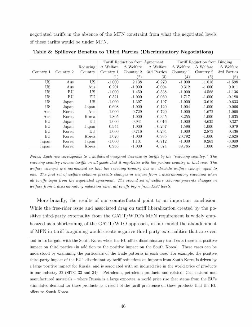
These findings are driven by and highlight an important difference across MFN and

discriminatory tariff bargaining that is quantified by our model: while we find that the

spillovers to third parties from tariff reductions negotiated in a bilateral are often large

in both the MFN and the discriminatory tariff bargaining settings, they are usually of

opposite signs, positive for MFN tariff bargaining and negative for discriminatory tariff

bargaining. As we show, the negative third-party externality associated with discrimina-

tory tariff reductions and the implied transfer of surplus from third parties to bargaining

parties drives down the levels of the negotiated tariffs in the absence of the MFN con-

straint from what these levels would be under MFN; and this force is sufficiently strong to

result in substantial over-liberalization of these tariffs. Put differently, while the free-rider

issue and associated drag on tariff liberalization created by the positive third-party exter-

nality from the GATT/WTO’s MFN requirement is widely emphasized as a shortcoming

of the GATT/WTO approach, we find that the abandonment of MFN in tariff bargaining

would create negative third-party externalities that are even more powerful, and that

would ultimately lead to tariff bargaining outcomes that are worse from the perspective

of world welfare.

Our work is related to other studies of trade policy in multi-country quantitative

trade models. Work of this kind includes Ossa (2014) and Ossa (2016), as mentioned

previously, and also Caliendo et al. (2017), Caliendo and Parro (2015), and Spearot (2016).

By comparison, a key distinguishing feature of our work is that we explicitly model the

bargaining process. We are thereby able to use our quantitative model of trade and

tariff bargaining to compare outcomes under MFN and counterfactual discriminatory

negotiations.

The remainder of the paper proceeds as follows. The next section sets out our quanti-

tative model of trade and tariff bargaining. Section 3 describes the data we use to estimate

8

the model, while section 4 describes our approach to estimation. Section 5 presents our

model estimates and computes a number of model benchmarks. Section 6 presents our

counterfactual. Section 7 concludes.

2 Model

Our model world economy consists of the multi-sector version of Eaton and Kortum

(2002) from Costinot et al. (2011), extended to include tariffs and to allow the parameter

governing the dispersion of productivity across varieties within a sector to vary by sector,

as in Caliendo and Parro (2015). The model world economy is then embedded into an

equilibrium model of tariff bargaining. In the next subsection, we describe the model

world economy, and in the following subsection we describe our approach to modeling

tariff bargaining.

2.1 Model World Economy

We consider a world economy with i = 1, ..., N countries and k = 1, ..., K sectors. Within

each sector k, there is a countably infinite number of varieties indexed by ω. We allow

each country to impose an import tariff (possibly discriminatory across trading partners)

in each sector k. Because our model world economy is a straightforward variant of the

models in Costinot et al. (2011) and Caliendo and Parro (2015), we provide only a minimal

description here, and refer readers to those papers for additional model details.

We begin by describing the supply side of the model. Each country has an immobile-

across-countries labor endowment Li. Production of each variety in each sector is governed

by a constant-returns-to-scale technology requiring only labor. Furthermore, an infinite

number of firms, all with the same productivity parameter, exist to produce each variety

in each sector, ensuring perfect competition.

The production technology for each variety is drawn from a Frechet distribution with

CDF given by

F ki (z) = exp

(−(

z

zki)−θk

),

where zki is country i’s sector-k level productivity parameter and θk is a sector-specific

productivity shape parameter. We will reference specific draws from these distributions as

9

zki (ω), that is, country i’s productivity in variety ω in sector k. While the first and second

moments of the distribution of productivity depend on both the z and the θ parameters,

the ratio of expected variety productivity for the same sector between two countries is

equal to the ratio of their zk parameters in sector k. Higher values of θk imply lower

heterogeneity in within-sector productivity, and more responsiveness of trade flows with

respect to changes in fundamentals (and hence higher trade elasticities) as a result.

Producers face iceberg trading costs and potentially tariffs when serving other coun-

tries. We parameterize iceberg costs to depend on an origin effect, a destination effect,

a sector-specific border effect, a sector-specific distance effect, and whether the origin

and destination share a common language, a physical border, or have a preferential trade

agreement (PTA). It is often noted that the so-called “Quad” countries of the US, the

(at the time) 10 member-countries of the EU, Canada and Japan had an outsized impact

on the shape of the Uruguay Round due to their status as major traders and special

trading relationships with each other. We attempt to capture this with inclusion of an

effect, common across sectors, for shipments between each of the Quad-country pairs.

Our parameterization of iceberg trade costs is then given by:

log dkji = αj + γi + β0k + β1kdistji + β2kPTAji + β3langji + β4borderji +∑n∈Q

β5nQuadn,ji

with dkji denoting the iceberg trade costs for country j’s sector-k exports to country i, and

with dkii = 1∀k. The variable distji is the distance between countries j and i, PTAji is an

indicator variable that takes the value 1 if countries j and i are members of a common

PTA and 0 otherwise, langji is an indicator variable that takes the value 1 if countries

j and i share a common language and 0 otherwise, borderji is an indicator variable that

takes the value 1 if countries j and i share a common physical border and 0 otherwise,

and Q is the set of pairs of the members of the “Quad,” i.e., the US, the EU, Canada

and Japan, and Quadn,ji is equal to one whenever countries j and i make up the pair n.

With perfect competition in each country-sector-variety, the price of each variety in each

country is equal to:

pki (ω) = minj∈1,...,N

wjzkj (ω)

dkji(1 + tkji)

10

where wj is the wage of labor in country j and tkji is equal to the ad valorem tariff levied

by country i on sector-k imports from country j.9

We now turn to the demand side of the model and describe the consumer demand

system. A representative consumer in each country chooses consumption levels of each

variety in each sector to maximize the following utility function that is CES across varieties

within a sector with a Cobb-Douglas aggregator across sectors:

ui = ΠKk=1(Ck

i )αki

Cki = (

∞∑ω=1

ck(ω)σ−1σ )

σσ−1 ,

where αki are country i’s taste parameters for sector k, and σ is a within-sector constant

elasticity of substitution across varieties. Consumers take prices for each variety as given.

They choose consumption to maximize this utility function subject to their budget con-

straint that total expenditure must be weakly less than their country’s labor income plus

tariff revenue.

We can now describe the equilibrium of the model given a set of tariffs. An equilibrium

consists of a vector of wages wi and a vector of national incomes Ei (wage income plus

tariff revenue) such that labor markets clear, trade is balanced, and consumers and firms

are behaving optimally.10

2.2 Tariff Bargaining

We assume that in a multilateral round of tariff negotiations, countries negotiate bila-

terally and simultaneously over tariff vectors. As we discussed in the Introduction, this

bargaining structure was featured in the first five GATT rounds of multilateral tariff ne-

gotiations, and it was used as a complement to multilateral bargaining methods in the

last three GATT rounds, including the Uruguay Round, as well as in the now-suspended

9With this specification we are assuming that the ad valorem tariff is applied to the delivered price

of the import good at the importing country’s border.10Countries do run trade deficits in the data which we can not rationalize in our static model. As

discussed in Ossa (2016), an ideal solution would involve a dynamic model of saving and borrowing which

is outside the scope of this paper. Ossa (2016) also discusses an alternative approach which partially

accounts for trade deficits by considering the trade surplus as fixed additional income to a country. We

instead simply abstract away from the issue of trade deficits and work in a setting of balanced trade.

11

WTO Doha Round. Moreover, as we also discussed in the Introduction, we will allow

countries to make use of costly transfers in their bargains, in order to capture the broader

set of issues beyond tariff bargaining that the Uruguay Round negotiations encompassed.

But for the moment we assume that bargaining takes place only over tariffs, and we pos-

tpone our description of the introduction of transfers into the model until after we have

described the basic tariffs-only bargaining structure.

As all tariffs affect all countries through the trade equilibrium in our model, the

payoffs from each bilateral negotiation depend on the outcomes of the other bilateral

negotiations. We follow Bagwell et al. (2017b) and apply the solution concept of Horn

and Wolinsky (1988) to this tariff bargaining problem. According to this solution, each

pair of negotiating countries maximizes its Nash product given the actions of the other

pairs.

Let πi(t) be the welfare of country i when the world vector of tariffs is given by t. We

measure a country’s welfare by its real national income level. When country i negotiates

with county j, they select the tariffs τ that they negotiate so as to maximize their Nash

product:

npij(τ, t−ij) = (πi(τ, t−ij)− πi(τ0, t−ij))ζij(πj(τ, t−ij)− πj(τ0, t−ij))1−ζij

where ζij is the bargaining power parameter of country i in its bilateral bargain with

country j and where we have partitioned the set of tariffs into those being negotiated

by i and j and all other tariffs as (τ, t−ij). τ0 represents the level for the tariffs under

negotiation between i and j that will prevail if i and j fail to reach an agreement. We

set these to be the levels of these tariffs in place when the negotiating parties entered the

round.

We further parameterize the pairwise bargaining powers. Specifically, each country has

a bargaining ability parameter ai. When countries i and j meet, the pairwise bargaining

parameter is equal to

ζij =exp (ai)

exp (ai) + exp (aj).

We now define the Horn and Wolinsky (1988) tariff bargaining equilibrium for our

model:

12

Definition 1 (Tariff Bargaining Equilibrium) An equilibrium in tariffs consists of a

vector of tariffs such that for each pair ij the tariffs negotiated by this pair maximizes npij

given the other tariffs in the vector.

The key assumption in the Horn and Wolinsky (1988) bargaining equilibrium is that,

when evaluating a candidate τ , the pair ij holds the vector t−ij fixed. In other words, if

ij were to not reach agreement, or were to deviate from a tariff vector specified by the

equilibrium, then the other tariffs do not adjust. As we discussed in the Introduction,

this equilibrium notion is sometimes referred to as “Nash-in-Nash,” because it is the

Nash equilibrium to the synthetic game where each pair constitutes a player, the payoff

function is the pair’s Nash bargaining product, and the strategies of each player are the

tariffs being negotiated by the pair associated with that player.

To reflect the tariff bargaining environment of the Uruguay Round, we introduce three

institutional constraints to our tariff bargaining solution11 First, we assume that countries

are restricted to bargain over MFN tariffs and cannot engage in bilateral bargains over

discriminatory tariffs.12 Second, we assume that countries are not allowed to make tariff

offers in any bilateral that would violate their existing GATT tariff bindings by exceeding

their bound (legal maximum) levels.13 And third, in line with the principal supplier rule

of GATT/WTO tariff negotiations, we assume that only the largest supplier of good k

into country i prior to the round can negotiate with country i over country i’s MFN tariff

in sector k, tmfnik .14

11Omitted from the institutional constraints that we impose on tariff bargaining is the GATT/WTO

norm of reciprocity. In the Conclusion, we discuss the possibility of augmenting our representation of the

Uruguay Round tariff bargaining protocol with the addition of a reciprocity norm.12GATT members can and do engage in bilateral bargains over discriminatory tariffs when they ne-

gotiate preferential trade agreements, which under the GATT/WTO rules contained in GATT Article

XXIV are permissible provided that the negotiating countries eliminate tariffs on substantially all trade

between them. And as Bagwell et al. (2017a) describe, in some of the early GATT rounds, the reach

of some of the bilaterals was expanded beyond negotiations over MFN tariffs to include discriminatory

(preferential) tariffs as well. But in the more recent GATT multilateral rounds, including the Uruguay

Round which is our focus here, negotiations were restricted to MFN tariffs.13In fact, under Article XXVIII of GATT, countries can engage in the renegotiation of their existing

tariff bindings and either modify in an upward direction or even withdraw these bindings. However, in

the multilateral rounds that are our focus here, which occur under Article XXVIIIbis, the purpose of

negotiations is to achieve reductions in the levels of tariff bindings, and tariff offers that violate existing

bindings would instead have to occur in the context of an Article XXVIII renegotiation and include the

bargaining partner with which the original tariff concession was negotiated.14In their examination of the bargaining data from the GATT Torquay Round, Bagwell et al. (2017a)

13

We now describe how we augment our model of tariff bargaining to include the pos-

sibility of costly international transfers. As discussed in the Introduction, there were a

number of important dimensions of the Uruguay Round negotiations that went beyond

tariff bargaining to specific issues such as agricultural subsidies, intellectual property,

services, and possibly even to broader non-economic issues covering national security

concerns and geopolitical affairs. To allow our model to reflect some of these broader

dimensions in the simplest way, we allow countries to make costly transfers as part of

their tariff negotiations. Let Πi(t,m) be the welfare of country i when the world vector

of tariffs is given by t and the world vector of net transfers is given by m. We continue to

measure each country’s welfare by its real national income level, but now augmented by

the net international transfer it receives. We model this as a direct utility transfer rather

than an income transfer, with no general equilibrium effects as a result: we think of this

as capturing the non-economic issues beyond the market access concerns associated with

tariff commitments that may have been at play during the negotiations.15

In this augmented setting, when country i negotiates with county j, the two countries

select the tariffs τ that they negotiate and the net transfer µij that country i pays to coun-

try j so as to maximize their Nash product, which we denote by NPij(τ, t−ij, µij,m−ij),

and which is given by:

(Πi(τ, t−ij, µij,m−ij)− Πi(τ0, t−ij, µ0,m−ij))ζij(Πj(τ, t−ij, µij,m−ij)− Πj(τ0, t−ij, µ0,m−ij))

1−ζij

where, as before, ζij is the bargaining power parameter of country i in its bilateral bargain

with country j and the set of tariffs has been partitioned into those being negotiated by

i and j and all other tariffs, (τ, t−ij), and where we now similarly partition the sets of

find that the average number of exporting countries bargaining with an importing country over a given

tariff was 1.25, suggesting that our assumption is a reasonable approximation. A potential caveat is that

the findings of Bagwell et al. (2017a) apply at the 6-digit HS level of trade, whereas here we are operating

at a more aggregate sectoral level; we return to this point in the Conclusion.15An alternative (and possibly complementary) approach to introducing transfers into our model would

be to allow international transfers of income. Transfers of this form would enter the budget constraint

of each country and have general equilibrium impacts, and this might better capture the economic issues

addressed during the Uruguay Round negotiations that went beyond tariff bargaining. Our approach is

simpler, and seems appropriate as a way to capture the non-economic issues described above that may also

have been at play in the Round. We leave to future research a more complete exploration of the various

ways that international transfers might be introduced into quantitative models of tariff bargaining.

14

transfers for countries i and j into those being negotiated by i and j and all other transfers,

(µij,m−ij). As before, τ0 represents the level for the tariffs under negotiation between

i and j that will prevail if i and j fail to reach an agreement, and we set these to be

the levels of these tariffs in place when the negotiating parties entered the round. And

similarly, µ0 represents the level of the transfer between i and j that will prevail if they

fail to reach agreement, which we set to zero.

Finally, to allow for the possibility of a non-zero cost of transfers, we assume that if

country i makes a positive net transfer to its bargaining partners in total (i.e., if∑

j µij >

0), then country i suffers an additional utility cost associated with orchestrating this level

of transfer equal to κ(∑

j µij)2. We treat the cost-of-transfers parameter κ as a parameter

to be estimated along with the bargaining power parameters of the model, and we estimate

as well the net transfers µij.

We then define the Horn and Wolinsky (1988) tariff-and-transfer bargaining equili-

brium for our model:

Definition 2 (Tariff-and-Transfer Bargaining Equilibrium) An equilibrium in ta-

riffs and transfers consists of a vector of tariffs and transfers such that for each pair ij

the tariffs and transfer negotiated by this pair maximizes NPij given the other tariffs and

transfers in the vector.

As noted above, to reflect the principal supplier rule of GATT/WTO tariff negotiati-

ons, we assume that only the principal supplier of good k into country i prior to the round

can negotiate with country i over country i’s MFN tariff in sector k, tmfnik . In the absence

of transfers, this in turn requires that a “double coincidence of wants” exists between any

viable pair of bargaining partners, in the sense that each country in the bargaining pair

must be a principal supplier of at least one good to the other country in the pair. With

the introduction of (costly) transfers, the requirement of a double coincidence of wants is

relaxed, in principle allowing more bargaining pairs to form; for example, if country A is

a principal supplier of good 1 into country B’s market, and country B is not a principal

supplier of any good into country A’s market, there could still be a viable bilateral bet-

ween countries A and B, in which country B offers to cut its tariff on good 1 in exchange

for a transfer from country A. For simplicity we do not allow the introduction of transfers

to expand the possible set of bilateral bargaining pairs in this way; in the Conclusion we

return to discuss how this added impact of the availability of transfers might affect our

results.

15

It is worth pausing here to consider how our estimation can pin down bargaining-power

parameters and the cost of transfers. If the Uruguay Round agreed tariffs correspond

closely to what according to our model would be the joint surplus maximizing tariffs for

each bilateral, then bargaining powers would be reflected in the transfers (which we don’t

observe) rather than the agreed tariffs, and we would have large standard errors on our

bargaining parameter estimates together with a low estimated cost of transfers. To the

extent that the Uruguay Round agreed tariffs do not correspond to what according to

our model would be the joint surplus maximizing tariffs for each bilateral, our estimation

will search for the combination of positive cost-of-transfers and bargaining powers that

generates predicted tariffs as close as possible to the Uruguay Round agreed tariffs.

3 Data

To operationalize our model, we require data on trade flows, production and value added,

and tariffs, all at the country-sector level. To quantify iceberg trade costs, we combine

these data with a set of data on gravity variables: distances between countries, whether

countries share a common language, and whether countries are members of a common

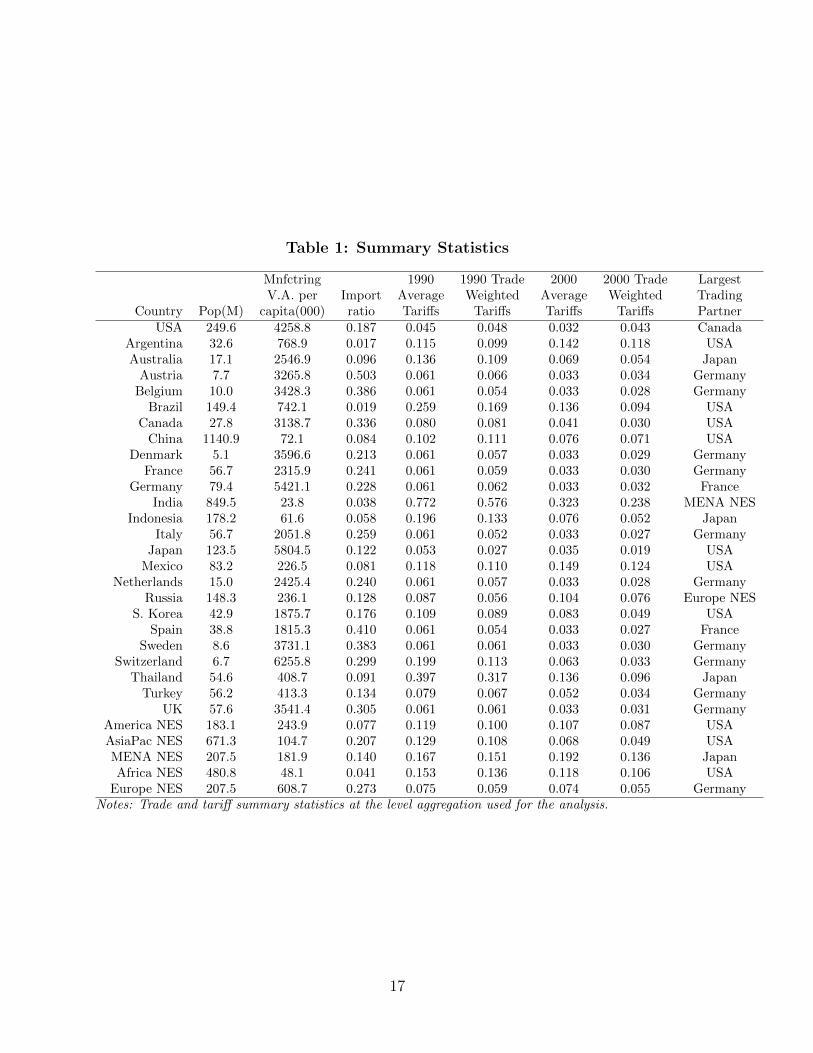
PTA. Details of the data cleaning and aggregation are contained in Appendix A. Table 1

provides summary statistics.

To represent the world economy, we include the twenty five largest countries by GDP

in 1990, and aggregate the rest of the world into one of five “not-elsewhere-specified”

(NES) regional entities: Americas, Asia-Oceania, Middle East-North Africa (MENA),

Africa, and Europe. We treat each regional entity as a sovereign individual country in

the estimation. We aggregate trade flows into 49 sectors. We began with SITC2 two-digit

codes, and then further combine several related sectors to arrive at a total of 49 traded

sectors.

3.1 Trade Flow, Production, and Value Added Data

The starting point for our data is the NBER world trade flows data from Feenstra et al.

(2005) for the year 1990. We compute the gross value in 1990 dollars of each country’s

imports from each other country at the sector level according to our country and sector

definitions. The NBER data do not provide information on a country’s production or

consumption. We impute each country’s sector-level production by extracting the ratio

16

Table 1: Summary Statistics

Mnfctring 1990 1990 Trade 2000 2000 Trade LargestV.A. per Import Average Weighted Average Weighted Trading

Country Pop(M) capita(000) ratio Tariffs Tariffs Tariffs Tariffs PartnerUSA 249.6 4258.8 0.187 0.045 0.048 0.032 0.043 Canada

Argentina 32.6 768.9 0.017 0.115 0.099 0.142 0.118 USAAustralia 17.1 2546.9 0.096 0.136 0.109 0.069 0.054 Japan

Austria 7.7 3265.8 0.503 0.061 0.066 0.033 0.034 GermanyBelgium 10.0 3428.3 0.386 0.061 0.054 0.033 0.028 Germany

Brazil 149.4 742.1 0.019 0.259 0.169 0.136 0.094 USACanada 27.8 3138.7 0.336 0.080 0.081 0.041 0.030 USA

China 1140.9 72.1 0.084 0.102 0.111 0.076 0.071 USADenmark 5.1 3596.6 0.213 0.061 0.057 0.033 0.029 Germany

France 56.7 2315.9 0.241 0.061 0.059 0.033 0.030 GermanyGermany 79.4 5421.1 0.228 0.061 0.062 0.033 0.032 France

India 849.5 23.8 0.038 0.772 0.576 0.323 0.238 MENA NESIndonesia 178.2 61.6 0.058 0.196 0.133 0.076 0.052 Japan

Italy 56.7 2051.8 0.259 0.061 0.052 0.033 0.027 GermanyJapan 123.5 5804.5 0.122 0.053 0.027 0.035 0.019 USA

Mexico 83.2 226.5 0.081 0.118 0.110 0.149 0.124 USANetherlands 15.0 2425.4 0.240 0.061 0.057 0.033 0.028 Germany

Russia 148.3 236.1 0.128 0.087 0.056 0.104 0.076 Europe NESS. Korea 42.9 1875.7 0.176 0.109 0.089 0.083 0.049 USA

Spain 38.8 1815.3 0.410 0.061 0.054 0.033 0.027 FranceSweden 8.6 3731.1 0.383 0.061 0.061 0.033 0.030 Germany

Switzerland 6.7 6255.8 0.299 0.199 0.113 0.063 0.033 GermanyThailand 54.6 408.7 0.091 0.397 0.317 0.136 0.096 Japan

Turkey 56.2 413.3 0.134 0.079 0.067 0.052 0.034 GermanyUK 57.6 3541.4 0.305 0.061 0.061 0.033 0.031 Germany

America NES 183.1 243.9 0.077 0.119 0.100 0.107 0.087 USAAsiaPac NES 671.3 104.7 0.207 0.129 0.108 0.068 0.049 USAMENA NES 207.5 181.9 0.140 0.167 0.151 0.192 0.136 JapanAfrica NES 480.8 48.1 0.041 0.153 0.136 0.118 0.106 USA

Europe NES 207.5 608.7 0.273 0.075 0.059 0.074 0.055 GermanyNotes: Trade and tariff summary statistics at the level aggregation used for the analysis.

17

of exports to total production at the country-sector level from the Global Trade Analysis

Project (GTAP) database, and we complement these data with manufacturing value added

data by country from UNIDO. Our measure of sector-level consumption by country is then

given by the difference between production and net exports.

3.2 Tariff Data

We obtain country-sector tariff equivalent applied MFN tariffs from the UNCTAD Trains

database on tariffs for 1990 and 2000. We use the 1990 applied tariffs as the pre-Uruguay

Round tariffs, and the 2000 applied tariffs as the negotiated outcomes from the Uruguay

Round.

There is an important distinction between the tariffs that countries actually apply to

imports into their markets, and the tariff bindings that they negotiate in the GATT/-

WTO.16 While introducing this distinction into a quantitative trade model would be a

very worthwhile project in its own right, it is well beyond the scope and focus of our

paper. In addition, as is well-known, the results of GATT/WTO tariff negotiating rounds

are typically phased in over an implementation period that can last a number of years. In

this regard the Uruguay Round was no exception, with phase-in periods ranging across

countries and sectors up to a maximum of roughly a decade. With the implementation

period of the Uruguay Round commencing on January 1 1995, our decision to use the dif-

ference between the applied tariffs in place in 1990 and the applied tariffs in place in 2000

as a measure of the negotiating outcomes of the round represents an attempt to capture

these complex features in a way that maintains the tractability of our quantitative model

and its use for studying tariff bargaining.

Finally, while we will estimate the parameters of our trade model utilizing data on

trade flows, production and value added, and tariffs for the full coverage of products, for

our bargaining analysis we focus attention on bargaining over tariffs for non-agricultural

16A tariff binding represents a legal cap on the tariff that a country agrees not to exceed when it applies

its tariff; the tariff it applies may be at the cap, but it may also be below the cap. For most industrialized

countries, the vast majority of applied tariffs are at the cap (Australia is a notable exception), but for

many emerging and especially developing countries, applied tariffs are often well below the cap (China

is a notable exception). A recent literature has begun to explore the value of tariff bindings that are set

above applied tariffs, and this literature finds that the reduction in uncertainty about worst-case (i.e.,

high-tariff) scenarios that such a binding implies can have large trade effects, e.g. Handley (2014) and

Handley and Limao (2015).

18

products (product categories 10-11 and 13-49 as defined in Table 9).17

3.3 Gravity Data

We use data on distances between countries, existence of preferential trading arrange-

ments, and a common language indicator from the Geography module of the CEPII

Gravity Dataset (Head and Mayer, 2014). This data set constructs distances between

countries based on distances between pairs of large cities and the population shares of

those cities. For the regional entities, we construct the distance with a partner as the

average distance between the countries forming the regional entity and the partner in

question. For two regional entities, we use the average distance across all pairs formed

with one country from each regional entity.

4 Estimation

We estimate the model in two steps. First, we estimate the taste, productivity, and ice-

berg cost parameters. Given these estimates, we then estimate the cost-of-transfers and

bargaining parameters. The reason for splitting the estimation process into two steps

is because the bargaining model is computationally much more intensive than the trade

model, as solving the bargaining model once involves potentially thousands of computa-

tions of a trade equilibrium at differing tariff levels. Because the trade model has several

thousand parameters, joint estimation with the bargaining model is prohibitively expen-

sive. For feasibility, we thus sacrifice some efficiency by not jointly estimating the trade

and bargaining/cost-of-transfers parameters. We do, however, allow the Uruguay Round

bargaining outcomes to inform our trade model estimates along one dimension: we in-

clude inequality moments in the trade model estimation reflecting the implication that

each bargaining pair in the Uruguay Round (based on the product-level principal supplier

status in our trade data) should generate a higher joint surplus with its observed Uruguay

Round agreed tariffs than if the pair had remained at its pre-Uruguay-Round tariff levels.

17The reason for not analyzing agricultural tariff changes is that many of the agricultural tariffs were

specific rather than ad-valorem. To operationalize the model, we require ad valorem tariffs. However, ad

valorem equivalents of specific agricultural tariffs display large fluctuations in levels due to world price

movements rather than tariff changes.

19

4.1 Non-linear least squares estimation of trade parameters

We estimate the model to minimize the distance between the data and the model’s pre-

dictions for (i) the ratio of each country’s imports from each other country in each sector

to the country’s total consumption in that sector, (ii) relative total value added across

countries, and (iii) for each bargaining pair, the difference between the pair’s joint surplus

at the observed post-Uruguay-Round tariffs and at the pre-Uruguay-Round tariffs on the

goods that are principally supplied by one member of the pair to the other member.

More specifically, the parameters to estimate consist of a vector of taste parameters

(α), a vector of productivity parameters (z), a vector of dispersion of productivity parame-

ters (θ), and a vector of iceberg cost parameters (β). Given the Cobb-Douglas preference

structure, the vector of taste parameters α can be inferred from the data directly as the

share of expenditure on each sector over total expenditure. Given these α estimates, we

then choose the remaining parameters to minimize the following criterion:

G(z, θ, β) =

xkij∑i xkij− xkij(z,θ,β)∑

i xkij(z,θ,β)∑

j,k xkij∑

j,k xkUSA,j

−∑j,k x

kij(z,θ,β)∑

j,k xkUSA,j(z,θ,β)

min (JSij(τPOSTij )− JSij(τ 0

ij), 0)

minz,θ,β

G(z, θ, β)′WG(z, θ, β)

where JSij(τPOSTij ) is the joint surplus of the negotiating pair of countries i and j evalu-

ated at the observed post-Uruguay-Round tariffs, and JSij(τ0ij) is the same joint surplus

evaluated at the observed post-Uruguay-Round tariffs for all tariffs other than those being

negotiated between the pair ij together with the pre-Uruguay-Round tariffs for the ta-

riffs being negotiated between the pair ij. The inequality moments associated with JSij

are implied by the Horn-Wolinsky bargaining equilibrium concept: if it were the case

that JSij(τPOSTij ) − JSij(τ

0ij) < 0, then the pair ij would have been better off with no

agreement. Evaluating the bargaining conditions increases the computational cost of the

estimation as it requires solving for equilibrium at several different tariff vectors. For this

reason, we include a subset of pairs motivated by size, trade flow patterns, and princi-

pal supplier relationships: US-EU, US-Japan, Canada-EU, Japan-EU, and Japan-South

Korea.18

18We construct the weighting matrix W as follows. The weights on the trade shares are 1. The trade

share difference between observed and reality can vary from -1 to 1, though most differences are on the

20

4.2 Discussion of Estimation and Data Variation

The non-linear mapping between trade shares, relative value added, and bilateral tariff

agreements that generate positive surplus into model parameters is difficult to characte-

rize formally. However, we now discuss the patterns in the data that help identify the

model’s parameters. We also compare our estimation approach to alternative estimation

approaches from the previous literature.

The sector level θk parameters govern the responsiveness of trade flows to changes in

the environment such as tariffs or productivities. Previous literature, such as Costinot

et al. (2011) and Caliendo and Parro (2015), derive linear estimating equations where

the left-hand-side variable is a non-linear transformation of bilateral trade flows at the

country pair-sector-direction level and the right-hand-side variable is a non-linear trans-

formation of either productivities (Costinot et al. (2011)) or tariffs (Caliendo and Parro

(2015)). The parameter θk is the coefficient on the right-hand-side variable in these for-

mulations.19 With these linear estimating equations, these papers pay special attention to

the identifying variation on the right hand side. Costinot et al. (2011) use an instrumen-

tal variables approach with additional data on productivities, while Caliendo and Parro

(2015) use a rich set of fixed effects to isolate variation in tariffs that is within country-

sector, and thus requires some countries to have discriminatory tariffs. These approaches

do have the benefit of clear attribution of the identifying variation being used to esti-

mate θ. That said, the log transformation of the left-hand-side variable entails dropping

pairs of countries which have zero trade flows from the estimation as discussed in Silva

and Tenreyro (2006). This approach also attributes idiosyncratic differences in a country

pair’s trade flows to iceberg costs and eliminates any role of measurement error in trade

flows.

The non-linear least squares approach that we employ uses the information conveyed

by pairs of countries which do not trade in a sector and allows for measurement error.

Furthermore, it delivers, in one step, estimates of iceberg costs and country-sector level

productivities that can be assessed against outside data sources and can be used to com-

order 0.01 or smaller. There are N*N*K=44100 of these. We weight the relative value added by 10.

There are 29 of these. Their scale can be arbitrarily large, but at the estimates, the differences are also

around 0.01 and smaller. Finally, we weight the five bargaining conditions by 105. Recall that these are

in utility units, and absent weighting are on the order of 10−4.19Caliendo and Parro (2015) allow for θ to vary at the sector level, while Costinot et al. (2011) restrict

θ to be constant across all sectors.

21

pute any counterfactual outcome in the domain of the model.20 The disadvantage of the

non-linear method is that it obscures the identifying variation being used to estimate θk

and does not lend itself to straightforward instrumental variable techniques. That said,

our estimation relies on patterns in the data which are similar to those relied on by the

previous literature, such as, conditional on observable components specified in the iceberg

costs, the covariance of trade shares with tariffs. The iceberg cost specification we employ

has separate origin, destination, and sector fixed effects, but not destination-sector fixed

effects. Therefore, identification does not hinge on observing discriminatory tariffs within

importing country-sector; instead, identification is achieved since MFN tariffs vary across

destinations for given sectors.

The bargaining conditions help ensure that the trade model parameters that we es-

timate are compatible with the observed tariff concessions from the Uruguay Round. In

this sense, we are using bargaining outcomes to help estimate the trade model parameters

such as the θk parameters. The trade model is point identified without these conditions,

and thus remains point identified after adding these inequalities to the criterion function.

The conditions we employ on the joint surplus are true for any bargaining power para-

meters. These conditions also have the potential to help allay concerns, were the model

to be mis-specified, about unobserved factors affecting import shares that are also corre-

lated with tariffs. To the extent that negotiations reflected beliefs about the world that

are supported by unbiased estimates of trade elasticities, then including the bargaining

conditions allows our estimates to incorporate that information.

4.3 Non-linear least squares estimation of cost-of-transfers and

bargaining parameters

With estimates of the trade model in hand, we estimate the cost-of-transfers parameter

and the bargaining parameters between pairs of countries in a second step. We again

employ non-linear least squares. Using the estimated trade parameters, we can solve

the bargaining model for predicted tariffs and net transfers given any cost-of-transfers

parameter and vector of bargaining parameters. We numerically search over the cost-

of-transfers parameter and bargaining parameters to minimize the distance between the

20Papers using the linear estimating equation approach are still able to run counterfactuals by using

the exact-hat algebra as in Dekle et al. (2008). This method allows one to estimate certain types of

counterfactual outcomes knowing only some aggregates rather than all of the model primitives.

22

observed tariff outcomes of the Uruguay Round and the tariff bargaining outcomes pre-

dicted by our model. In other words, we estimate the cost-of-transfers and bargaining

parameters by solving the following:

minκ,a

Σi,k(τki (κ, a)− τ ki )2

where τ ki (κ, a) is the model’s prediction for country i’s MFN tariff in sector k for a

candidate cost-of-transfers parameter κ and vector of bargaining parameters a, and τ ki is

the observed MFN tariff of country i in sector k in the year 2000.

5 Model Estimates

5.1 Trade Parameter Estimates

Table 2 presents the within-country dispersion of productivity parameter estimates by

sector, ordered by descending θk (descending trade elasticity). Our estimates of θk display

substantial heterogeneity across sectors. According to our estimates, the three highest-θk

sectors are Live animals (40.87), Miscellaneous edible products and preparations (24.44)

and Petroleum (22.38), while the three lowest-θk sectors are Pharmaceuticals (4.36), Metal

Ores (4.13) and Textile fibres (3.98). Our average θ across sectors is 10.77.

The range of estimates in the literature is arguably quite wide and comparison from

paper to paper is difficult due to different degrees of product or geographical aggregation.

That said, the Eaton and Kortum (2002) estimate of θ across sectors is 8.28. Costinot

et al. (2011) estimate 6.53. Caliendo and Parro (2015) estimates an aggregate θ of 4.55

with a range from 50.01 (Petroleum) to 0.37 (Other transport). Ossa (2014) estimates a

mean of 3.42 with a range from 10.07 (Wheat) to 1.19 (Other animal products). Overall,

the θ values we estimate tend to be somewhat higher than the current consensus in the

literature, a feature that is driven partly by including conditions from the bargaining

model in estimating the trade model parameters. In particular, we find that while the

bargaining conditions are not binding at the estimated parameters, there is another set of

parameters that would deliver a lower objective function value if one ignores the bargaining

conditions. This other parameter vector features θ estimates which are 34% lower on

average than the estimates with the bargaining conditions in place, and which are closer

to the estimates in the literature. However, at these estimates, the bargaining model does

not predict tariff changes well for any bargaining parameters.

23

The estimated average iceberg cost across all sectors and country-pairs is 109.0%. The

average-across-sectors incurred iceberg cost is 75.3% as lower iceberg cost country pairs

trade with each other more. These iceberg costs estimates are smaller than other estimates

in the literature. For example, Novy (2013) finds an average iceberg cost of 108% for a

group of developed countries in 1990. For the same countries, our estimates indicate an

average unweighted iceberg cost of 69.2%. The lower estimated levels of iceberg costs

that we find relative to the literature is consistent with our finding as well of higher θ

estimates relative to the literature, in that observed levels of trade can be matched by

modifying θ or iceberg costs. That is, if for example the model is under-estimating the

amount of trade relative to the data, one can decrease iceberg costs or decrease θ.

Table 2: θ Estimates by Industry.

Sector θ SE Sector θ SELive animals 40.87 2.10 Footwear 8.50 5.12Misc. Edible 24.44 10.75 Chemical 8.32 5.03

Petroleum 22.38 11.31 Non-metallic mineral manufactures 8.31 8.00Dairy 21.77 10.22 Crude rubber 8.09 4.73

All others 18.45 9.45 Office machines 8.02 3.42Cereals 17.16 5.86 Specialized Machinery 7.82 4.15

Feeding stuff 16.94 7.19 Pulp and waste paper 7.77 2.10Plumbing, heating and lighting 15.86 6.18 Crude materials,n.e.s. 7.74 3.31

Furniture and parts thereof 15.03 7.75 Travel goods and bags 7.67 3.80Paper manufactures 11.98 10.67 Road vehicles 7.51 4.03Electrical machinery 11.91 3.91 Meat 7.50 3.64Wood manufactures 11.82 6.63 Non-ferrous metals 7.42 3.89Vegetables and fruit 11.78 8.01 Fertilizers 7.32 4.91

Beverages 11.73 1.71 Tobacco 7.15 4.31Misc manufactures 10.92 4.28 Fabrics 7.07 4.36

Rubber manufactures 10.81 5.49 Organic chemicals 6.99 5.25Animal oils and fats 10.63 3.29 Iron and steel 6.94 5.87

Coffee, Tea, Spices 10.46 10.30 Scientific instruments 6.91 3.63Power generating machinery 10.23 4.99 Other transport equipment 6.42 4.13

Inorganic chemicals 10.19 5.42 Seafood 5.67 3.83Hides and skins 9.44 4.59 Coal 5.38 1.65

Sugar 9.35 3.52 Pharmaceutical 4.36 1.29Cork and wood 9.07 5.63 Metal Ores 4.13 0.92

Resins 8.94 4.97 Textile fibres 3.98 0.98Dyeing and tanning 8.78 4.85

Notes: Non-linear least squares estimates of θ by sector in descending order of estimate.

With regard to cross-country fundamental productivity levels, Figure 1 plots the distri-

bution of estimated productivity levels for each country. Productivity levels are positively

correlated across sectors, so the higher productivity countries in agriculture also tend to

be the higher productivity countries in manufacturing.

24

As a test of the model, we compare the estimated wage levels across countries to wage

data from the Bureau of Labor Statistics International Labor Comparisons (ILC) program

for 1997. For the 19 countries we could match to these data, a regression of the model’s

predicted relative wage on the relative wage in the data produces a coefficient estimate

of 0.933 with associated standard error of 0.157. The estimated R2 for this regression is

0.674. While we did not use any wage data in estimating the model, the implied estimated

wage rates are not systematically biased estimates and can account for about two-thirds

of the cross-country variation.

Figure 1: Productivity Distributions by Country

0

0.5

1

1.5

2

2.5

Estim

ate

d P

roductivity

United S

tate

s

Arg

entina

Austr

alia

Austr

ia

Belg

ium

Bra

zil

Canada

Chin

a

Denm

ark

Fra

nce

Germ

any

India

Indonesia

Italy

Japan

Mexic

o

Neth

erlands

Russia

South

Kore

a

Spain

Sw

eden

Sw

itzerland

Thaila

nd

Turk

ey

United K

ingdom

Am

erica N

ES

Asia

/Oceania

NE

S

ME

NA

NE

S

Afr

ica N

ES

Euro

pe N

ES

Notes: For each country, the target is the median estimated productivity across sectors. The box represents

the interquartile range. The line represents the full range. Each sector in the US is normalized to a

productivity level one.

5.2 Model Benchmarks

We compute various benchmarks implied by the 1990-based estimated trade model. Table

3 reports the results. We begin with the first and second columns of Table 3, which report

respectively the changes in welfare that would result if, with regard to all products, the

world reverted to autarky, or if all iceberg costs (including tariffs) were removed. These

25

Table 3: Model Benchmarks

Zero TotalIceberg Free Welfare

Country Autarky Costs Trade Maximizing NashUnited States -1.76% 18.82% 0.03% -1.13% -0.21%EU -5.44% 47.28% 0.00% -1.62% -0.01%

Austria -10.20% 58.09% 0.00% -2.01% -0.02%Belgium -17.05% 79.49% -0.04% -1.63% 0.00%Denmark -5.19% 90.64% -0.02% -1.47% -0.01%France -4.98% 64.75% -0.01% -1.08% -0.02%Germany -2.86% 29.75% -0.06% -2.10% 0.03%Italy -5.07% 44.12% -0.05% -2.08% 0.00%Netherlands -11.74% 85.97% 0.05% -1.77% -0.02%Spain -6.42% 62.85% 0.02% -1.79% 0.01%Sweden -8.92% 51.38% 0.00% -1.78% -0.06%United Kingdom -4.61% 36.92% 0.15% -0.86% -0.07%

Argentina -1.20% 107.26% 0.11% 0.66% -0.08%Australia -3.31% 103.94% 0.20% 1.67% 0.09%Brazil -1.14% 86.00% 0.10% 1.52% -0.08%Canada -6.88% 51.62% 0.07% 0.35% -0.21%China -2.41% 52.99% 0.60% 1.27% -0.01%India -2.44% 89.39% 0.53% 3.16% 0.12%Indonesia -2.35% 76.23% 0.34% 0.67% -0.07%Japan -1.81% 23.45% 0.20% 0.85% 0.06%Mexico -2.67% 59.80% 0.01% 0.32% -0.06%Russia -3.52% 75.16% 0.21% 0.83% -0.49%South Korea -5.11% 54.65% 0.42% 1.45% -0.03%Switzerland -5.78% 60.00% -0.05% -0.12% 0.01%Thailand -4.98% 152.18% 0.70% 2.86% 0.04%Turkey -3.43% 59.62% -0.12% -0.15% 0.05%America NES -3.88% 119.63% 0.28% 6.55% -0.29%Asia/Oceania NES -5.58% 58.74% 0.77% 2.39% -0.41%MENA NES -5.45% 94.58% 0.29% 1.13% -0.90%Africa NES -2.20% 55.41% 0.13% 2.58% -0.19%Europe NES -5.46% 43.00% 0.92% 2.95% -0.61%Total Welfare -3.42% 47.26% 0.17% 0.25% -0.10%

Notes: Estimated model’s predicted percentage change in national welfare from estimated 1990 status quo

for benchmark scenarios. In column 1, we set iceberg costs for all countries in all sectors to 5000%,

effectively shutting down trade across countries. In column 2, we set iceberg costs to zero for all countries

in all sectors. In column 3, we set all non-agricultural tariffs for the US, Australia, EU, Japan, and

South Korea to zero. These four countries and the EU make up the set of negotiating countries based

on principal supplier status according to our estimates. In column 4, we solve for the total welfare

maximizing levels of non-agricultural tariffs for the five negotiating countries. In column 5, we compute

a Nash equilibrium in non-agricultural tariffs for the five negotiating countries. Tariffs in columns 4 and

5 are non-discriminatory.

26

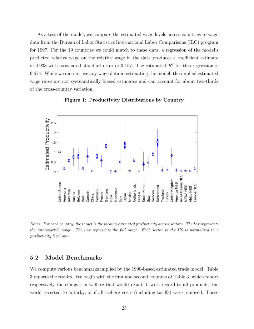
are standard benchmarks in the quantitative trade modeling literature, and are useful for

positioning the broad predictions from our quantitative trade model within that literature.

We find that, relative to welfare under the status-quo 1990 tariffs, moving to autarky

would reduce total world welfare by 3.42%, while eliminating iceberg costs would raise

total world welfare by 47.26%. For the US, moving to autarky reduces country welfare by

1.76% which is somewhat larger than the 0.7% to 1.4% range computed by Arkolakis et al.

(2012) under the assumption of a single trade elasticity in the range of 5 to 10 applied

to all sectors. This number is lower, however, than the 13.5% estimated in Ossa (2015),

despite the fact that our model also features heterogeneity in θ across sectors. Several

features account for the difference between our predictions and Ossa’s. Ossa’s estimates

are based on a model with 251 sectors for the base year 2007 whereas our model has 49

sectors and is estimated using data from the base year 1990 (Ossa reports an estimate

for the US of 8.9% based on a more aggregated 28 sector calculation). Ossa also reports

a trade-weighted cross-industry average trade elasticity of 2.94, substantially lower than

that implied by our θ estimates.

We will also be interested in how the Horn-Wolinsky solution of our model compares

to a benchmark tariff bargain that reached the efficiency frontier. There are no market

imperfections or political economy forces in our model, and so achieving free trade in

all tariffs would place the world on the efficiency frontier. But as a benchmark with

which to compare our model outcomes, global free trade is not particularly meaningful,

both because our bargaining analysis is limited to tariffs on non-agricultural products, and

because according to our model under the principal supplier rule not all countries engaged

in tariff bargaining in the Uruguay Round. A more meaningful free-trade benchmark with

which to compare the Horn-Wolinsky solution of our model is a bargain that sets to zero

just the non-agricultural tariffs under negotiation in the Uruguay Round according to

our model. It is also meaningful to consider an alternative benchmark that sets these

same tariffs equal to the levels that would maximize world welfare in light of the existing

distortions implied by the fixed levels of all other tariffs in the world. Similarly, for

assessing how the Horn-Wolinsky solution of our model compares to a benchmark Nash

tariff war, we solve for the non-cooperative Nash tariff equilibrium over this same set of

tariffs, holding all other tariffs fixed at their 1990 levels.

The third, fourth and fifth columns of Table 3 report benchmark welfare effects un-

der these free-trade, world-welfare maximizing and Nash benchmarks, respectively. In

particular, for the benchmark results reported in these three columns, we limit the tariff

27

changes to those tariffs on non-agricultural products that were imposed by the set of

negotiating countries in the Uruguay Round, defined as the set of countries that by their

principal supplier status in 1990 according to our model had at least one viable bilateral

bargaining partner in the Uruguay Round (i.e., a partnership where each country was the

principal supplier of at least one product into the other country’s market). We refer to

the resulting set of tariffs as the set of tariffs that were “under negotiation in the Uruguay

Round.”

The third column of Table 3 reports the welfare results from reducing all the tariffs

that were under negotiation at the Uruguay Round from their 1990 levels to zero, with

all other tariffs held fixed at their 1990 levels. World welfare rises by 0.17%, an amount

that is smaller than the findings in Ossa (2014)) who predicts a rise in total welfare of

0.5%. However, Ossa’s prediction reflects the impact of eliminating all tariffs, whereas as

we have noted above our prediction is about the impact of eliminating only the subset of

(non-agricultural) tariffs that were under negotiation in the Uruguay Round based on the

set of viable bilateral bargaining partners given principal supplier patterns in 1990.

The fourth column of Table 3 reports results when we solve for the levels of the tariffs

negotiated in the Uruguay Round that would maximize total world welfare, corresponding

to the utilitarian/Benthamite point on the (constrained) efficiency frontier. World welfare

under these tariff levels is higher than world welfare under our free trade benchmark for

two reasons. First, there are pre-existing distortions associated with the tariffs not under

negotiation at Uruguay which remain fixed at their 1990 levels under both exercises,

and in the presence of these pre-existing distortions some deviation from free trade for

the remaining tariffs is optimal from the perspective of world welfare: in particular,

we find that on average the world-welfare maximizing benchmark entails further tariff

liberalization than the free trade benchmark (i.e., on average, import subsidies are needed

to offset the trade restricting effects of the tariffs not under negotiation at Uruguay).21

And second, the terms of trade effects of utilitarian tariffs redistribute income towards

higher marginal utility of income countries.22

21This finding may be interpreted using the Lerner symmetry theorem. Specifically, given the pre-

existing distortions associated with import tariffs not under negotiation in the Uruguay Round, an efficient

outcome could be achieved if export policies were available so that each country could offset the effects

of foreign import tariffs with appropriately selected export subsidies. We do not allow countries to use

export policies in our model; however, due to the Lerner symmetry theorem, a country can similarly

offset the effects of foreign import tariffs with appropriately selected import subsidies.22At equal wages, the marginal utility of income is higher in countries with lower price indices. All

28

The fifth column of Table 3 reports the welfare results from increasing all the tariffs

that were under negotiation in the Uruguay Round from their 1990 levels to their Nash

equilibrium levels, with all other tariffs held fixed at their 1990 levels. Here we find that

total welfare decreases for most countries relative to their welfare under status-quo tariffs,

but a few countries would enjoy small gains due to favorable terms-of-trade movements

as a result of the Nash trade war. In aggregate the decrease in total welfare amounts to

0.1%. This reflects the fact that our estimated losses from a move to autarky are relatively

modest (as is true for much of the quantitative trade modeling literature), that the move

to Nash tariffs is only allowed for products that were under negotiation in the Uruguay

Round, and that the Nash tariffs are sizable but far from prohibitive. US tariffs rise on

average from 4.44% to 9.4%. EU tariffs rise on average from 5.82% to 11.31%. Japanese

tariffs rise from 5.03% to 12.6%. Ossa (2014)) finds Nash tariffs averaging 63% and an

aggregate loss of 2.9% from a trade war relative to status-quo tariffs. In addition to the

fact that our Nash calculations refer to only those tariffs that were under negotiation

in the Uruguay Round whereas Ossa’s Nash calculations cover all tariffs, the differences

between our Nash results and Ossa’s also reflect differing estimated trade elasticities, with

Ossa’s estimates again indicating less responsiveness of trade to tariffs on average than

our estimates. The estimates of Markusen and Wigle (1989), who find Nash tariff rates

for the US and Canada of 18% and 6% respectively and small losses from a trade war

relative to free trade, are more in line with our numbers.

Together our estimates in the third and fifth columns of Table 3 suggest that, begin-

ning from Nash tariffs, the GATT rounds up to but not including the Uruguay Round

had achieved by 1990 roughly 40% of the potential aggregate world-wide gains from the

complete elimination of the tariffs that were under negotiation in the Uruguay Round.

Compared to a benchmark that sets these same tariffs equal to the levels that would

maximize world welfare in light of the existing distortions implied by the fixed levels of

all other tariffs in the world as of 1990, the fourth and fifth columns of Table 3 suggest

that, beginning from Nash tariffs, the GATT rounds leading up to the Uruguay Round

achieved roughly a third of the aggregate world-wide welfare gains that were possible with

changes to the tariffs under negotiation in the Uruguay Round.

else equal, larger and/or more centrally located countries thus may be expected to have higher marginal

utilities of income. Since in our model countries do not have sufficient policy instruments with which to

effect lump-sum transfers, the utilitarian calculus balances the benefits of such redistribution against the

associated distortion costs.

29

5.3 Cost-of-Transfers and Bargaining Parameter Estimates

We now turn to our second step and estimate the cost-of-transfers and bargaining pa-

rameters. As described above, our approach is to use our trade model to solve for the

Horn-Wolinsky bargaining outcomes beginning from 1990 tariff bindings and respecting

MFN and the principal supplier rule, and to search over cost-of-transfers and bargaining-

power parameters to minimize the distance between the observed tariff outcomes of the

Uruguay Round and the tariff bargaining outcomes predicted by our model. We let the

model predictions regarding principal supplier status guide our set of bilateral bargains.

For reference, the top panel of Table 4 displays the observed pattern of principal

supplier status at the level of product aggregation in our data. For this table, we have

combined the (at the time of the Uruguay Round) 10 EU member countries into the

EU, because these countries negotiated their (common external) GATT Uruguay Round

tariff commitments as a bloc; and to focus on the major traders, we have omitted from

the table the 5 regional NES entities. Also, in defining the principal suppliers relevant

for Uruguay Round negotiations, for the numbers in this table we have netted out trade

with fellow PTA members (e.g., US exports to Canada are excluded when calculating the

identity of principal suppliers into Canada). For each cell in the table, the first entry

gives the number of products for which the column country is the principal supplier into

the row country, and the second entry gives the number of products for which the row

country is the principal supplier into the column country. The top panel of Table 4

records 12 country-pairs where both entries are non-zero (highlighted in the table with

square brackets around those entries), reflecting the double coincidence of wants that can

support a bilateral tariff negotiation between the pair. The 12 pairings involve 6 countries:

the 4 Quad members – the US, the EU, Canada and Japan – and two additional countries,

Australia and South Korea.

According to our trade model estimates, the predicted pattern of principal supplier

status for the same set of countries is displayed in the bottom panel of Table 4. As

the bottom panel of Table 4 reflects, the principal supplier relations predicted by our

model capture 7 of the 12 pairings in the data and involve 5 of the 6 countries: three of

the four Quad members, US, EU and Japan, and the two additional countries Australia

and South Korea. This seems to capture the main bilaterals in the Uruguay Round

(US-EU, US-Japan, EU-Japan, Japan-South Korea) but misses some others that are

potentially important (e.g., EU-Canada). Overall, our current set of bargaining countries

includes the 14 major industrialized countries that were arguably the key actors in the

30

Table

4:

Pri

nci

pal

Suppli

er

Rela

tionsh

ips

US

Arg

enti

na

Au

stra

lia

EU

Bra

zil

Can

ad

aC

hin

aIn

dia

Ind

on

esia

Jap

an

Mex

ico

Ru

ssia

Kore

aS

wit

zerl

an

dT

hailan

dU

SA

rgen

tin

a12,0

Au

stra

lia

[11,2

]0,1

EU

[25,2

6]

0,1

1[1

,21]

Bra

zil

9,0

0,0

0,0

11,0

Can

ad

a0,0

0,0

[1,1

][3

0,3

]0,0

Ch

ina

4,0

0,0

2,0

15,0

0,0

1,0

Ind

ia8,0

0,0

1,0

21,0

0,0

0,0

0,0

Ind

on

esia

6,0

0,0

4,0

12,0

0,0

0,0

0,0

0,0

Jap

an

[18,5

]0,0

[3,3

][1

3,3

]0,0

0,3

0,1

20,2

0,1

0M

exic

o35,0

0,0

0,0

2,0

0,0

0,0

0,0

0,0

0,0

0,0

Ru

ssia

0,0

0,0

1,0

33,0

0,0

1,0

0,0

0,0

0,0

0,0

0,0

Kore

a[1

3,2

]0,0

[2,1

][4

,2]

0,0

0,1

0,0

0,0

0,2

[17,4

]0,0

0,0

Sw

itze

rlan

d0,0

0,0

0,0

39,0

0,0

0,0

0,1

0,0

0,0

0,1

0,0

0,0

0,0

Th

ailan

d7,0

0,0

0,0

13,0

0,0

0,0

0,0

0,0

0,0

14,0

0,0

0,0

2,0

0,0

Tu

rkey

3,0

0,0

0,0

34,0

0,0

0,0

0,0

0,0

0,0

0,0

0,0

0,0

1,0

0,0

0,0

US

Arg

enti

na

Au

stra

lia

EU

Bra

zil

Can

ad

aC

hin

aIn

dia

Ind

on

esia

Jap

an

Mex

ico

Ru

ssia

Kore

aS

wit

zerl

an

dT

hailan

dU

SA

Arg

enti

na

17,0

Au

stra

lia

[20,1

]0,0

Eu

rop

e[3

0,2

4]

0,1

70,7

Bra

zil

9,0

0,0

0,0

17,0

Can

ad

a0,0

0,0

1,0

27,0

0,0

Ch

ina

3,0

0,0

2,0

19,0

0,0

0,0

Ind

ia3,0

0,0

1,0

25,0

0,0

0,0

0,0

Ind

on

esia

2,0

0,0

4,0

19,0

0,0

0,0

0,0

0,0

Jap

an

[28,9

]0,0

0,8

[7,3

]0,0

0,5

0,1

10,2

0,8

Mex

ico

0,0

0,0

2,0

28,0

0,0

0,0

0,0

0,0

0,0

1,0

Ru

ssia

3,0

0,0

0,0

32,0

0,0

0,0

0,0

0,0

0,0

0,0

0,0

Kore

a4,0

0,0

[2,2

][1

6,2

]0,0

0,0

0,2

0,0

0,0

[14,2

]0,1

0,1

Sw

itze

rlan

d1,0

0,0

0,0

37,0

0,0

0,0

0,0

0,0

0,0

0,0

0,0

0,0

0,0

Th

ailan

d3,0

0,0

2,0

21,0

0,0

0,0

0,0

0,0

0,0

7,0

0,0

0,0

0,0

0,0

Tu

rkey

1,0

0,0

0,0

36,0

0,0

0,0

0,0

0,0

0,0

0,0

0,0

0,0

0,0

0,0

0,0

Note

s:T

he

top

pan

elpre

sen

tspri

nci

pal

suppli

erre

lati

on

ship

sacc

ord

ing

toth

edata

.T

he

bott

om

pan

elre

pre

sen

tspri

nci

pal

suppli

erre

lati

on

ship

sacc

ord

ing

toth

etr

ade

mod

elat

the

esti

mate

dpa

ram

eter

vect

or.

For

each

cell

inth

eta

ble,

the

firs

ten

try

give

sth

en

um

ber

of

pro

du

cts

for

whic

hth

eco

lum

nco

un

try

isth

epri

nci

pal

suppli

erin

toth

ero

wco

un

try,

an

dth

ese

con

den

try

give

sth

en

um

ber

of

pro

du

cts

for

whic

hth

ero

wco

un

try

isth

epri

nci

pal

suppli

erin

toth

eco

lum

nco

un

try.

For

the

nu

mbe

rsin

this

tabl

e,tr

ade

wit

hfe

llow

PT

Am

embe

rshas

been

net

ted

ou

t.S

quare

brack

ets

indic

ate

the

bila

tera

lre

lati

on

ship

sw

her

ebo

then

trie

sare

posi

tive

.

31

tariff negotiations of the Uruguay Round (the exclusion of Canada from this set being

potentially the most important omission, mitigated to some degree by the fact that the

US and Canada did not engage in bilateral negotiations over MFN tariffs in the Uruguay

Round due to the existence of the US-Canada FTA and subsequently NAFTA).23

Table 5 displays the bargaining parameter estimates for each of the negotiating coun-

tries,24 as well as the estimated cost-of-transfers parameter κ. Two points are clear from

Table 5.

Table 5: Bargaining Model Parameter Estimates

Country Bargaining Parameter SEUSA 0 -

Australia -10.981 0.174EU -12.017 0.224

Japan 6.841 0.453South Korea -3.349 0.928

Parameter SECost of Transfers Coefficient 277.613 0.928

Notes: Estimated bargaining parameters (ai) and coefficient on quadratic transfer cost. The parameter

for the US is normalized to 0.

First, transfers were possible in the Uruguay Round, but they were not costless. The

point estimate of κ reported in Table 5 translates into an average cost of transfers amoun-

ting to 84.68% when evaluated at the mean level of net transfers paid by countries who

made positive net transfers. That is, according to our estimates, on average a country

wishing to transfer 1 unit of utility to a bargaining partner in the Uruguay Round gave

up 1.8468 units of utility to do so. And averaged across those countries making positive

net transfers, the marginal cost of the last unit of utility transferred rises to 129.06%.

The second point that is clear from Table 5 is the relative ranking of bargaining powers,

with Japan the strongest bargainer followed in descending order by the US, South Korea,

Australia and the EU. As we describe further in the next subsection, Japan’s strong

23As we noted earlier, we do not allow the possibility of (costly) transfers to relax the requirement of a

principal-supplier-based “double coincidence of wants” for each viable bargaining pair. But a comparison

of the entries in the top and bottom panels of Table 4 suggests that allowing this expanded definition

of viable bargaining pairs might improve the match between the set of bilateral bargaining partners in

the model and those suggested by the principal supplier relationships in the data. We return in the

Conclusion to discuss this as a possible direction for future research.24Because the same constant could be added to each bargaining parameter without changing predicti-

ons, we normalize the US bargaining parameter to zero.

32

bargaining position manifests itself in our model as Japan receiving large tariff concessions

from its bargaining partners while making tariff concessions and non-tariff transfers that

were small in comparison to the benefits it received. The EU’s weak bargaining position

leads it to agree to both relatively large tariff cuts and positive transfers in its bilaterals.

Interpreting the estimates in Table 5 requires some caution. A naive interpretation of

the bargaining parameters as relative “power” between the pairs can be misleading. These

parameters reflect how the two negotiating countries split the marginal surplus that can

be obtained by their agreement conditional on all other bilateral negotiation outcomes.

Here we are relying heavily on the Horn-Wolinsky bargaining solution structure, which

pins down the particular disagreement point from which the marginal surplus of a bila-

teral agreement is defined. A country could have strong bargaining power in each of its

bilaterals and nevertheless fare poorly in the Uruguay Round relative to the 1990 status

quo if the outcomes from all other bilaterals have served to disproportionately worsen this

country’s disagreement payoff in each of its bilaterals. Alternatively, a country could fare

well as a result of the Uruguay Round outcomes relative to its welfare in the 1990 status

quo, and yet be revealed to have very weak bargaining power in a given bilateral where

the disagreement payoff had moved strongly in its favor.25

While the bargaining parameter estimates do reflect how evenly the surplus from the

bilateral tariff bargain is split between the two parties, in our tariff-bargaining setting

these parameters also reflect an additional feature, namely, the slope of the bilateral

bargaining frontier. Our cost-of-transfers estimate indicates that countries did not have

access to lump-sum transfers in the Uruguay Round, and so utility is not transferable

across countries and the slopes of the bilateral bargaining frontiers will typically not be

equal to −1. Instead, with the countries in any bilateral using tariff changes combined

with costly transfers to transfer utility between them, the slope of the bargaining frontier

in any given bilateral will reflect the cost of transfers and the relative degree to which the

incidence of each country’s tariff changes falls on, and only on, its bilateral bargaining

partner.26

25Of course, if the actual disagreement point in a bilateral deviates significantly from that under the

Horn-Wolinsky bargaining solution, the implied split and hence the implied bargaining parameters could

be different.26If countries were bargaining over a sufficiently complete set of trade taxes, they would be able to use

adjustments in these trade taxes to transfer surplus between them in a lump-sum manner. For example, in

a two-good two-country general equilibrium setting, Mayer (1981) shows that adjustments in the import

tariff in each country that preserve the equality of the relative price in each country can effect lump-sum

33

Figure 2: US and EU Welfare Fron-tier

US Welfare

EU

Wel

fare

Disagreement PointNegotiated Agreement

Figure 3: EU and Japan WelfareFrontier

Japan Welfare

EU

Welfare

Disagreement Point

Negotiated Agreement

Notes: These curves represents the frontier of feasible welfare pairs for the US-EU bilateral (left panel)

and Japan-EU bilateral (right panel) negotiations holding the other pairs fixed at the equilibrium outcomes.

The dashed line has slope equal to minus one.

Figures 2 and 3 illustrate this feature for the US-EU and Japan-EU bilaterals. The

bilateral bargaining frontier in each figure is constructed by optimally adjusting the tariffs

under negotiation in that bilateral and the costly transfer between the two negotiating

countries, holding all other tariffs and transfers fixed at their predicted agreement levels,

to shift surplus between the two countries. As Figure 2 depicts, the slope of the bargaining

frontier between the US and the EU is essentially linear but steeper than -1 throughout

the relevant range, indicating that the tariffs (and transfer) negotiated in this bilateral

were more effective at shifting surplus from the US to the EU than in the other direction.

This means in turn that for any given bargaining parameter for the US-EU bilateral, the

division of the surplus under the Nash bargaining solution will be shifted in the direction

of the EU relative to what it would be if the slope of the bilateral bargaining frontier

were -1 throughout. Figure 3 reveals that the bargaining frontier between Japan and the

EU is more clearly concave over the relevant range, and takes on a slope of -1 at a point

that favors the EU relative to Japan, indicating that in the Japan-EU bilateral, the tariffs

under negotiation were more effective at shifting surplus from Japan to the EU.

In Table 6, we present evidence suggesting that asymmetries in market power, the

position of the initial tariffs relative to their best-response levels, and the spillovers to

third parties are all factors in understanding the slopes of the bilateral bargaining frontiers.

transfers across countries. This is infeasible in the bilaterals under study in the present setting, because

the set of import tariffs under negotiation do not constitute a sufficiently complete set of trade taxes.

34

Consider for example, the first two rows of this table, which relate to the US-Australia

bilateral. With all other tariffs positioned at their agreed levels as predicted by our

model, the first three columns of Table 6 report that, beginning from the US-Australia

negotiated agreement tariffs as predicted by our model, when the US lowers its tariffs

under negotiation in this bilateral by an amount that reduces its welfare by 1 unit, it

increases the surplus of all other countries by 6.271 units, with Australia receiving 2.677

units and third parties receiving the remaining 3.594 units. By contrast, beginning from

these same tariffs, when Australia lowers its tariffs under negotiation in this bilateral by

an amount that reduces its welfare by 1 unit, it increases the surplus of all other countries

by 0.467 units, with the US receiving 0.083 units and third parties receiving the remaining

0.384 units.

Table 6: Spillover Benefits to Third Parties (MFN Negotiations)

Tariff Reduction from Agreement Tariff Reduction from BindingReducing ∆ Welfare ∆ Welfare ∆ Welfare ∆ Welfare ∆ Welfare ∆ Welfare

Country 1 Country 2 Country Country 1 Country 2 3rd Parties Country 1 Country 2 3rd Parties(1) (2) (3) (4) (5) (6)

US Aus US -1.000 2.677 3.594 -1.000 3.285 4.520US Aus Aus 0.083 -1.000 0.384 0.090 -1.000 0.398US EU US -1.000 1.557 1.231 -1.000 2.516 2.144US EU EU 0.335 -1.000 1.410 0.405 -1.000 1.728US Japan US -1.000 1.166 0.712 -1.000 2.240 1.347US Japan Japan 0.501 -1.000 0.460 0.576 -1.000 0.564

Aus Korea Aus -1.000 0.731 3.909 1.000 0.048 0.240Aus Korea Korea 0.786 -1.000 1.015 0.725 -1.000 1.134EU Japan EU -1.000 0.609 0.677 -1.000 15.438 19.550EU Japan Japan 0.739 -1.000 0.573 1.495 -1.000 1.382EU Korea EU -1.000 0.513 4.766 1.000 0.160 1.361EU Korea Korea 0.783 -1.000 1.972 0.928 -1.000 2.658

Japan Korea Japan -1.000 0.826 1.555 1.000 0.629 1.103Japan Korea Korea 0.991 -1.000 1.275 5.723 1.000 8.413

Notes: Each row corresponds to a unilateral marginal decrease in tariffs by the “reducing country.” The

reducing country reduces tariffs on all goods that it negotiates with the partner country in that row. The

welfare changes are normalized so that the reducing country has an absolute welfare change equal to one.

The first set of welfare columns presents changes in welfare when all tariffs begin from the negotiated

agreement. The second set of welfare columns presents changes in welfare when all tariffs begin from

1990 levels.

These asymmetric effects reflect a combination of factors. The feature that the US

tariff cuts generate substantially more surplus gains for the rest of the world overall

than do Australia’s tariff cuts when Australia and the US make the above-described

tariff cuts reflects in part the differences across these two countries in import volumes and

35

market power over world prices with respect to the products on which they are bargaining.

Another factor is the relative distance of the agreed tariffs from best-response levels for

the tariffs over which these two countries bargain; this factor governs the magnitude of the

described tariff cuts.27 And the feature that Australia captures a greater portion of the

rest-of-world gains generated by the US’s tariff cuts (roughly 43%) than is captured by the

US when Australia makes the described tariff cuts (roughly 18%) reflects asymmetries in

the degree of dominance that each country’s principal suppliers play in serving the other

country’s markets.

The last three columns of Table 6 report analogous measures, but do so beginning from

the bargaining pairs’ disagreement (1990) tariffs rather than from the pairs’ negotiated

agreement tariffs (with all other tariffs also positioned at their 1990 levels). Similar

asymmetric effects arise from this starting point and have similar interpretations, but

now it is possible that unilateral tariff reductions can increase a country’s welfare (if the

1990 levels for the tariffs it negotiates in this bilateral are above its best-response levels

in light of the 1990 levels of all other tariffs) and, because these calculations do not begin

from a point on the bilateral bargaining frontier, could (but need not) increase the welfare

of all countries.

Notably, the third-party spillovers reported in both columns 3 and 6 of Table 6 are

uniformly positive. While the overall surplus gain for the rest of the world generated by

an importing country’s MFN tariff cuts is expected to be positive due to the induced

terms-of-trade effects, the sign of the spillovers to individual countries is not guaranteed

to be positive, and depends on trade patterns. That is, while the sum of the impacts on

the bargaining partner and third parties should be positive when an importing country

reduces its import tariffs as part of a bilateral bargain, the impact on third parties taken

as a group could be positive or negative and is ultimately an empirical question for which

columns 3 and 6 of Table 6 provide an answer.28

This point was emphasized by an early study commissioned by GATT which became

known as the Haberler Report. Written by a Panel of Experts that included Roberto de

Oliveira Campos, Gottfried Haberler, James Meade and Jan Tinbergen, the purpose of the

27For example, if a country’s agreed tariffs were at their best-response levels, then an envelope argu-

ment ensures that small tariff reductions would have no first-order effect on that country’s welfare. This

suggests that a country may need to make larger tariff cuts to generate a 1 unit welfare reduction when

that country’s tariffs are positioned closer to their best-response levels.28In fact, even the overall impact could in principle be of either sign in a multi-product environment,

depending on the signs and strengths of the interactions across products.

36

report was to investigate the prevalence of agricultural protectionism and “...the failure

of the export trade of the under-developed countries to expand at a rate commensurate

with their growing import needs.” (Campos et al., 1958). The issue of spillovers was

explained by the Report in these terms:

The problem of the interests of different primary producing countries outside

industrialized Western Europe and North America is ... not only a question

which of the other countries would gain by a moderation of agricultural pro-

tectionism in these two great industrialized regions; there are undoubtedly

cases in which an increase in agricultural protectionism in these two regions,

while it would be to the disadvantage of some of the unindustrialized countries,

would actually be to the advantage of others. ... An increased stimulus to the

production of wheat in any of the countries of North America or of Western

Europe by increasing the exportable surplus of North America and decreasing

the import requirements of Western Europe would depress the world mar-

ket for wheat. This might mean that a country like India or Japan would

obtain cheaper imports of wheat (either because of a fall in the world price or

because of a development of special sales or gifts for the disposal of surplus

wheat by the United States), but a country like Australia or the Argentine

which competed in the world export market for wheat would be damaged. ...

In general, if one considers any particular agricultural product, a protective

stimulus to its production in any one country by increasing supplies relatively

to the demand for that product will tend to depress the world market for that

product. This will damage the interests of other countries which are exporters

of the product on the world market. But it will be to the national interest of

countries which import the product from world markets. Whether the initial

protective stimulus confers a net benefit or a net damage to all other countries

concerned depends, therefore, upon whether the country giving the protective

stimulus to its own production is an exporter or an importer of the product;

if it is an exporter it is conferring a benefit on the world by giving its supplies

away at a cheap price; if it is an importer it is damaging the rest of the world

by refusing to take their supplies. (Campos et al. (1958), footnotes omitted).

In the context of bilateral MFN tariff bargaining, the general principle described by

the Haberler Report describes well the pattern of externalities that each bilateral bargain

37

has to confront. Based on this principle, we would expect the overall surplus gain for the

rest of the world generated by an importing country’s MFN tariff cuts to be positive, and

this is confirmed in the results reported in Table 6. What is also confirmed by the results

in Table 6 is that both the bargaining partner, and third parties as a group, each gain

from the importing-country MFN tariff cuts being negotiated in the Uruguay Round.

5.4 MFN Tariff Bargaining in the Uruguay Round

Comparing our Horn-Wolinsky model solution to the actual Uruguay Round tariff

bargaining outcomes, we find that we can explain 57.86% of the variation in 190 tariffs

under negotiation in the Uruguay Round using our cost-of-transfers parameter and four

bargaining parameters. The welfare impacts of the Round’s MFN tariff bargaining as

predicted by our model are presented in the first and second columns of Table 7. The first

column reports the impact of the negotiated tariff cuts predicted by our model, while the

second column includes as well the impacts of the net transfers negotiated according to

our model as part of the Round.29

The total world welfare gain from the Round reported in Table 7 is small in magnitude,

which is not surprising in light of our benchmark findings presented in columns 3 and 4 of

Table 3 that, beginning from their 1990 levels, the gains in world welfare are small from

eliminating all tariffs under negotiation in the Uruguay Round or from setting these tariffs

at their world welfare maximizing levels (0.17% and 0.25% respectively). That said, our

Horn-Wolinsky model solution indicates that in increasing total world welfare by 0.11%,

the Uruguay Round achieved roughly 40% of the potential aggregate world-wide welfare

gains in moving from the non-cooperative Nash tariff levels to this free-trade benchmark,

and it achieved roughly a third of the world-wide welfare gains beginning from Nash that

would have been possible under world-welfare maximizing levels of these tariffs. Overall,

and recalling that our focus is on the tariffs under negotiation in the Uruguay Round,

our model indicates that the GATT rounds leading up to the Uruguay Round and the

Uruguay Round itself together achieved roughly two thirds of the potential aggregate

world-wide welfare gains in moving from the non-cooperative Nash to the world-welfare

maximizing benchmark, leaving roughly a third of the potential world welfare gains from

29Transfers are determined at the aggregate level for the EU. For the purposes of Table 7, we allocate

transfers to member countries of the EU directly in proportion to population.

38

Table 7: Estimated Uruguay Round and Counterfactual Outcomes

MFN No MFNTariffs

Average Tariffs -46.95% -47.43%Weighted Average Tariffs -54.50% -48.96%

Country Welfarewith with

transfers transfersUnited States 0.00% 0.04% 0.03% 0.09%EU 0.04% 0.02% -0.03% -0.05%

Austria 0.07% 0.05% -0.02% -0.04%Belgium 0.01% 0.00% 0.00% -0.01%Denmark 0.02% 0.00% -0.04% -0.05%France 0.03% 0.00% 0.05% 0.03%Germany 0.00% -0.01% -0.09% -0.10%Italy 0.02% -0.02% 0.01% -0.02%Netherlands 0.05% 0.03% 0.02% 0.01%Spain 0.07% 0.02% -0.07% -0.10%Sweden 0.06% 0.04% 0.02% 0.00%United Kingdom 0.14% 0.12% -0.03% -0.04%

Argentina 0.05% 0.05% -0.02% -0.02%Australia 0.08% 0.04% 0.22% -0.03%Brazil 0.05% 0.05% -0.02% -0.02%Canada 0.00% 0.00% -0.10% -0.10%China 0.35% 0.35% -0.10% -0.10%India 0.31% 0.31% -0.06% -0.06%Indonesia 0.14% 0.14% -0.05% -0.05%Japan 0.21% 0.20% 0.29% 0.28%Mexico 0.00% 0.00% -0.04% -0.04%Russia 0.07% 0.07% -0.04% -0.04%South Korea 0.47% 0.43% -1.86% -2.02%Switzerland -0.04% -0.04% -0.07% -0.07%Thailand 0.42% 0.42% -0.07% -0.07%Turkey -0.08% -0.08% -0.06% -0.06%America NES 0.11% 0.11% 0.02% 0.02%Asia/Oceania NES 0.36% 0.36% -0.16% -0.16%MENA NES 0.06% 0.06% -0.08% -0.08%Africa NES 0.05% 0.05% -0.02% -0.02%Europe NES 0.40% 0.40% -0.12% -0.12%Total Welfare 0.12% 0.11% 0.00% -0.01%

Notes: Each column represents changes in the row relative to the pre-Uruguay tariff levels. The first

set of columns represents the Horn-Wolinsky MFN solution at the estimated bargaining parameters. The

second set of columns represents the Horn-Wolinsky discriminatory solution at the estimated bargaining

parameters.

39

negotiating over this set of tariffs as “unfinished business.”30

The first two columns of Table 7 also reveal that there is significant variation in the

gains from the Uruguay Round’s MFN tariff bargaining across the member countries, with

substantially higher than average gains going to a number of emerging and developing

countries and smaller gains going to some of the industrialized countries. Among the

emerging and developing economies with especially high gains are China (who was not

a GATT member at the time of the Uruguay Round but enjoyed MFN treatment from

the EU and the US), India, Thailand and the regional entities in Asia/Oceana NES and

Europe NES. These countries were not among our bargaining pairs and hence these gains

reflect favorable terms-of-trade movements as a result of the Round. Turning to the

industrialized countries, the US gains are relatively small, amounting to a little less than

half of the average gains experienced by countries as a result of the Round, while the EU

gains are even smaller once the EU net transfers to bargaining partners are accounted

for. And Australia’s gains are comparable to those of the US, once its large net transfer

payments to bargaining partners are taken into account. Japan enjoys above average

gains, but it is South Korea that enjoys the largest gains of any country from the Round.

Of special interest are the results for Japan reported in Table 7. Japan’s gains from

the Round are above-average, but they are substantially smaller than those of South

Korea, despite the fact that as we observed earlier our bargaining parameter estimates

indicate that Japan is the strongest bargainer, with South Korea only possessing moderate

bargaining power. This apparent contradiction is resolved by noting that here we are

comparing how countries fared in the Uruguay Round relative to their 1990 welfare levels,

while the bargaining power parameters reflect how well a country does in each of its

bilateral bargains relative to the Horn-Wolinsky disagreement point for that bilateral.

Evidently, Japan’s strong bargaining position is reflected in the fact that it did extremely

well in its bargains relative to the Horn-Wolinksy disagreement points for those bargains,

but the Horn-Wolinsky disagreement points moved in an unfavorable direction for Japan

relative to the 1990 status quo.

It is interesting to note that, according to our model predictions, not all countries

gained from the Uruguay Round. In particular, we find that Switzerland and Turkey

30It is also interesting to note from a comparison of column 2 of Table 7 and column 4 of Table 3 that,

under the world welfare maximizing benchmark, much of the increased gains relative to the negotiated

MFN tariff cuts would go to developing and emerging economies, as might be expected given that these

countries were not among the bargaining pairs in the Uruguay Round and hence their interests were not

directly represented in those bilateral bargains.

40

suffer losses. As these two countries were not among our bargaining pairs and hence do

not alter their own tariffs from 1990 levels, the losses they suffer as a result of the Uruguay

Round reflect adverse terms-of-trade movements that resulted according to our model

from the negotiated MFN tariff cuts of others. This illustrates the point highlighted in

the Haberler Report and discussed above, that the MFN tariff reductions of each country

are expected to generate positive effects for the rest of the world taken as a whole, but

need not lead to positive effects for every country in the rest of the world.

Also interesting are losses that are theoretically possible but that we do not find.

While under Nash-in-Nash bargains each bilateral negotiation must lead to an agreement

which, with the outcomes of all other negotiations taken as given, benefits both negotia-

ting parties, the externalities across bargaining pairs raise the possibility that a country

engaged in bargaining could nevertheless be made worse off as a result of the web of bi-

lateral tariff bargains negotiated in the multilateral round than it would have been if the

round had never taken place. That said, all the bargaining parties in our representation

of the Uruguay Round did benefit from the negotiations, as the second column of Table 7

reflects. Some EU member countries were slightly worse off, but the EU as a whole enjoys

a small welfare improvement, as we have noted.

6 Counterfactual

As we have described above, under our representation of the Uruguay Round bargaining

protocol, our results point to the existence of unfinished business in tariff liberalization

with respect to the tariffs under negotiation in the Uruguay Round, in line with the under-

liberalization possibility identified by Bagwell et al. (2017b) when negotiations proceed

over MFN tariffs. This raises the possibility that changes to the protocol that stimulate

further negotiated tariff liberalization could be attractive from the perspective of world

welfare. In particular, in light of the potential drag on tariff liberalization generated

by the positive third-party externalities associated with MFN tariff cuts as reported in

Table 6, could the abandonment of MFN have allowed countries to achieve greater tariff

liberalization than occurred under the MFN restriction, and in so doing have allowed the

Uruguay Round to achieve greater gains in world welfare? And would the distribution of

the gains from the Uruguay Round across countries have been impacted in a substantial

way had the MFN requirement not been in place? We now turn to these and other

counterfactual questions, by comparing the outcomes from the Uruguay Round with the

41

outcomes that would be predicted by our model had the Uruguay Round negotiations

occurred under a bargaining protocol that abandons the MFN requirement.

To this end, recall that, in addition to allowing countries to make costly transfers

as part of their tariff negotiations, we have represented the Uruguay Round bargaining

protocol with three institutional constraints, namely, that countries (i) are restricted

to bargain over MFN tariffs, (ii) must respect existing GATT tariff commitments and

not raise their tariffs above these commitments, and (iii) abide by the principal supplier

rule, which guides each importing country to limit its negotiations on a given product

to the exporting country that is the largest supplier of that product to its market. We

now consider an alternative bargaining protocol under which the first and third of these

constraints are removed and countries can negotiate discriminatory tariff bargains. Our

primary interest is in how relaxation of the MFN requirement impacts tariff bargaining,

and as the principal supplier rule was introduced into the GATT bargaining protocols

in order to facilitate bilateral tariff bargaining in the presence of MFN, it is natural to

consider removing these two constraints at the same time. Because the model does not

perfectly predict tariffs under our representation of the Uruguay Round protocol, we

compare simulated outcomes under the counterfactual protocol to simulated outcomes

under our representation of the Uruguay Round protocol rather than to the observed

post-Uruguay tariffs.

To predict outcomes under discriminatory negotiations, we again solve for a bargai-

ning equilibrium with our estimated bargaining parameters. In the discriminatory case,

however, each pair negotiates only over tariffs that they will apply to each other. These

bilateral tariff bargains still affect the welfare of third countries because they affect pro-

duction and consumption patterns in the trade equilibrium, but they lack the direct effect

of altering tariffs on third countries automatically through MFN, and so the third-party

effects will be different from the MFN case. More specifically, while we would expect and

Table 6 confirms that the overall rest-of-world effect of a unilateral MFN tariff reduction

is positive, and while as Table 6 confirms we also find a positive third-party effect from a

country’s unilateral MFN tariff reductions agreed within a bilateral, the third-party effect

of an analogous unilateral discriminatory tariff reduction agreed within a bilateral is likely

to be negative, and the implied transfer of surplus from third parties to bargaining parties

is then likely to drive down the levels of these negotiated tariffs in the absence of the MFN

constraint from what the negotiated levels of these tariffs would be under MFN, even as

the liberalizing impact of the resulting tariff reductions are not automatically broadened

42

by extension to apply to other trading partners under the MFN requirement.31

To isolate the intensive-margin impact that the third-party effects of discriminatory

tariff reductions have on tariff bargaining outcomes in our model, we consider a counter-

factual in which, for each country, the set of its tariffs being negotiated is constrained to

include only the sectors that were negotiated by that country in the Uruguay Round, and

the set of countries negotiating on these tariffs is constrained to include only the countries

that it negotiated with in the Uruguay Round. That is, if county A was negotiating an

MFN tariff cut on sector j imports with the principal supplier of sector-j exports into

its market, then in our counterfactual country A is allowed to negotiate a discriminatory

tariff cut on sector-j imports with each of the countries that it bargained with in the

Uruguay Round and that also export sector-j goods to its market. But we do not allow

additional extensive margin effects on the pattern of bargaining.

The third and fourth columns of Table 7 present the results of this counterfactual,

with the third column presenting the welfare implications associated with the negotiated

discriminatory tariff changes and the fourth column presenting the welfare implications

once the negotiated transfers are also included. In the absence of MFN the average

tariff under negotiation drops by 47.43% while under MFN it drops by 46.95%. This

comparison, however, masks the degree to which countries are incentivized to negotiate

deeper tariff cuts when those cuts can be discriminatory. The added inducement to

negotiate tariff cuts when MFN is abandoned is brought into sharp relief when the No-

MFN averages are calculated over only the product-and-country pairs that were also in

play under MFN: as expected, under this calculation, the average tariff under negotiation

when MFN is abandoned drops by 107.35% as compared to a drop of 46.95% when MFN is

in place. But a comparison across the first two columns (MFN) and the third and fourth

columns (No MFN) of Table 7 also reveals that the MFN negotiations are better for

world welfare than discriminatory negotiations. More specifically, we would expect from

the findings of Bagwell et al. (2017b) that in the absence of an MFN rule Nash-in-Nash

tariff bargaining always results in inefficient over-liberalization, but what the findings

in Table 7 indicate is that the degree of inefficient over-liberalization according to our

model is sufficiently important to outweigh the inefficient under-liberalization that arises

31Intuitively, negotiated tariffs are likely to be lower in the absence of the MFN constraint than in

the presence of the MFN constraint for the following reason: starting at their negotiated MFN tariffs,

if two countries were allowed to use discriminatory tariffs, then they could jointly gain from exchanging

(perhaps small) discriminatory tariff cuts with each other, since they thereby could enjoy a transfer of

surplus from third parties due to the implied world-price movements.

43

according to the model under MFN, resulting in worse outcomes for total world welfare

under discriminatory tariff bargaining than under MFN tariff bargaining. In fact, as the

third and fourth columns of Table 7 indicate, our findings suggest that discriminatory

tariff bargaining would have wiped out all the gains in total world welfare associated with

MFN tariff bargaining, leaving total world welfare essentially at its 1990 level.

In principle, both the over-liberalization of tariffs and any additional tariff discrimi-

nation that results from discriminatory tariff bargaining could play a role in the poor

performance of this bargaining protocol when judged on the basis of world welfare.32 To

assess quantitatively the roles played by these two features for our findings reported in

Table 7, we recalculate the trade equilibrium at two sets of tariffs which vary the degree

of discrimination while maintaining average levels of tariffs. First, setting the MFN tariffs

of the negotiating countries in each sector equal to the average negotiated discriminatory

tariff for that country and sector, and thereby eliminating any tariff discrimination that

arose as a result of the discriminatory tariff bargaining, we find that world welfare would

increase by 0.04%. And second, in a similar vein, setting the discriminatory tariffs that

the negotiating countries apply to other negotiating countries in each sector equal to the

average negotiated discriminatory tariff among the negotiating countries in that country

and sector, and thereby eliminating tariff discrimination among the negotiating countries

that arose as a result of the discriminatory tariff bargaining, we find that total world

welfare would increase by 0.03%. Both of these calculations result in gains that are lower

than those under the MFN negotiations reported in Table 7 (0.11%) and higher than those

under the discriminatory negotiations reported in Table 7 (-0.01%), and the calculations

suggest that roughly one third of the poor performance of the discriminatory tariff bar-

gaining protocol is attributable to the tariff discrimination that results from bargaining,

with the remaining two thirds attributable to over-liberalization.

Turning to the impact of the abandonment of MFN on the distribution of gains across

countries, Table 7 shows that developing and emerging countries are among the biggest

losers from the abandonment of MFN, in some cases (e.g. China, India, Asia/Oceana

NES and Europe NES) faring substantially worse than under the 1990 status quo. Among

industrialized countries, South Korea suffers the largest losses from the abandonment of

32For example, it is possible that discriminatory tariff bargaining could lead to inefficient over-

liberalization with no tariff discrimination in equilibrium, if all countries were symmetric along the

relevant dimensions, but with various asymmetries it is natural to expect that both over-liberalization

and tariff discrimination would contribute to the poor performance of a discriminatory-tariff bargaining

protocol.

44

MFN, experiencing a 2.02% reduction in welfare relative to the 1990 status quo level, and

the EU and Canada also lose. By contrast, the US and some of the EU-member countries

enjoy small gains from the abandonment of MFN, but our results indicate that Japan

would be by far the biggest gainer.

In fact, Japan’s large welfare gain from the abandonment of MFN and South Ko-

rea’s large welfare loss are linked, with South Korea’s welfare loss heavily influenced by

Japanese outcomes: re-running the discriminatory counterfactual, but excluding Japan

from all negotiations, we find that South Korea’s welfare loss would be only 0.4%. This

Japan-South Korea linkage reflects two key features. Japan has high bargaining power,

and Japan shares strong similarities to South Korea in geographic location and industry

specialization. In particular, with regard to the first feature, as we have observed, our

estimates indicate that Japan was the strongest bargainer among negotiating partners

at the Uruguay Round, and this translates into an ability to extract deep MFN tariff

cuts from its bargaining partners in the presence of MFN, and deep discriminatory ta-

riff cuts from its bargaining partners when MFN is abandoned. Japan’s large gain from

the abandonment of MFN stems in part from its enhanced ability to exploit its strong

bargaining power when the constraint of MFN is lifted. With regard to the second fea-

ture mentioned above, the estimated sector productivity parameters for Japan and South

Korea have a correlation of 0.79 whereas the mean, across countries, correlation is 0.5;

and South Korea is the most correlated country for Japan and Japan is the second most

correlated country, after China, for South Korea. Thus, Japan’s strong bargaining power

leads to low tariffs for South Korean exporters under MFN, as South Korean exporters

compete closely with Japanese exporters for the same markets and therefore enjoy the

same low MFN tariffs; and with the abandonment of MFN, Japan’s strong bargaining

power leads to favorable discriminatory outcomes for Japan which now hurt South Korea

exporters.

Table 8 provides analogous information to Table 6 but now for the counterfactual case

of discriminatory tariff bargaining. The most striking difference across the two tables is

in the spillovers to third parties, which for MFN tariff bargaining are uniformly positive

as we have noted but which for discriminatory tariff bargaining are now almost always

negative.33 It is this negative third-party externality that is driving down the levels of the

33There are two exceptions to the pattern of negative third-party externalities displayed in Table 6:

beginning from the 1990 tariff bindings, in its bargain with the US when Australia offers discriminatory

tariff cuts there is a small positive impact on third parties (in addition to the positive impact on the US),

45

negotiated tariffs in the absence of the MFN constraint from what the negotiated levels

of these tariffs would be under MFN.

Table 8: Spillover Benefits to Third Parties (Discriminatory Negotiations)

Tariff Reduction from Agreement Tariff Reduction from BindingReducing ∆ Welfare ∆ Welfare ∆ Welfare ∆ Welfare ∆ Welfare ∆ Welfare

Country 1 Country 2 Country Country 1 Country 2 3rd Parties Country 1 Country 2 3rd Parties(1) (2) (3) (4) (5) (6)

US Aus US -1.000 2.138 -0.270 -1.000 11.018 -1.598US Aus Aus 0.201 -1.000 -0.004 0.312 -1.000 0.011US EU US -1.000 1.450 -0.538 -1.000 4.588 -1.136US EU EU 0.521 -1.000 -0.060 1.717 -1.000 -0.180US Japan US -1.000 1.397 -0.197 -1.000 3.619 -0.633US Japan Japan 0.608 -1.000 -0.120 1.004 -1.000 -0.066

Aus Korea Aus -1.000 0.729 -0.720 1.000 1.672 -1.060Aus Korea Korea 1.805 -1.000 -0.345 8.255 -1.000 -1.635EU Japan EU -1.000 0.941 -0.016 -1.000 4.635 -0.327EU Japan Japan 0.944 -1.000 -0.267 1.596 -1.000 -0.079EU Korea EU -1.000 0.716 -0.294 -1.000 2.873 0.436EU Korea Korea 1.026 -1.000 -0.985 20.792 -1.000 -2.628

Japan Korea Japan -1.000 1.101 -0.712 -1.000 9.263 -3.009Japan Korea Korea 0.936 -1.000 -0.374 89.785 1.000 -8.289

Notes: Each row corresponds to a unilateral marginal decrease in tariffs by the “reducing country.” The

reducing country reduces tariffs on all goods that it negotiates with the partner country in that row. The

welfare changes are normalized so that the reducing country has an absolute welfare change equal to

one. The first set of welfare columns presents changes in welfare from a discriminatory reduction when

all tariffs begin from the negotiated agreement. The second set of welfare columns presents changes in

welfare from a discriminatory reduction when all tariffs begin from 1990 levels.

More broadly, the results of our counterfactual point to an important conclusion.

While the free-rider issue and associated drag on tariff liberalization created by the po-

sitive third-party externality from the GATT/WTO’s MFN requirement is widely emp-

hasized as a shortcoming of the GATT/WTO approach, in our model the abandonment

of MFN in tariff bargaining would create negative third-party externalities that are even

and in its bargain with the South Korea when the EU offers discriminatory tariff cuts there is a positive

impact on third parties (in addition to the positive impact on the South Korea). These cases can be

understood by examining the particulars of the trade patterns in each case. For example, the positive

third-party impact of the EU’s discriminatory tariff reductions on imports from South Korea is driven by

a large positive impact for Russia, and is associated with an induced rise in the world price of products

in our industry 22 (SITC 33 and 34) – Petroleum, petroleum products and related; Gas, natural and

manufactured materials – where Russia is a large exporter, a world price rise that stems from the EU’s

stimulated demand for these products as a result of the tariff preference on these products that the EU

offers to South Korea.

46

more powerful, and ultimately lead to tariff bargaining outcomes that are worse from the

perspective of world welfare.

7 Conclusion

This paper embeds a quantitative model of world trade into a model of bilateral bargaining

over tariffs to examine the welfare effects of the most-favored-nation (MFN) requirement

that characterizes negotiations at the GATT/WTO. We estimate the model using trade

flows from 1990 and tariff outcomes from the Uruguay Round of GATT/WTO negotia-

tions. As emphasized in the theoretical literature, the welfare effect of imposing MFN

and thereby ruling out discriminatory tariff bargaining is ambiguous and depends on trade

patterns. In a trade model whose parameters are estimated to match observed trade flows,

we quantify a free-rider issue and associated drag on tariff liberalization that is created by

the positive third-party externality from the MFN requirement and that leads to under

liberalization relative to efficient outcomes, but our results indicate that the abandonment

of MFN in tariff bargaining would create negative third-party externalities that are even

more powerful and that would lead to substantial over liberalization. On balance we find

that MFN tariff negotiations are superior to discriminatory tariff negotiations in terms of

increasing world-wide welfare for this reason.

There are several promising avenues for future research. An obvious direction is to

expand the current framework to allow for more products, that is, to handle a more dis-

aggregated product classification. While this is essentially a computational challenge, it

is an important extension, as actual tariff negotiations occur at a much more disaggregate

level than the (essentially 2 digit) level that we have modeled here, and greater disag-

gregation could have important impacts on the principal supplier status that is central

in shaping the bargaining patterns of the Round and associated externalities. Relatedly,

as we noted above, while we allow bargaining partners to exchange costly transfers as

part of their bilateral tariff negotiations, we do not allow this exchange of transfers to

relax the double-coincidence-of-wants requirement that bargaining only over tariffs would

imply. Allowing the presence of costly transfers to have this extensive-margin impact on

bargaining could have important impacts on the bargaining outcomes.

Also important is to consider the possibility that countries bargained under an ad-

ditional constraint in the Uruguay Round, namely, that of reciprocity. Bagwell et al.

(2017a) review historical and institutional evidence that reciprocity was a significant con-

47

straint in GATT tariff negotiating rounds, and they identify a number of the stylized

facts emerging from the GATT Torquay Round bargaining data that can be interpreted

as consistent with bilateral tariff bargaining under a reciprocity constraint (and MFN).

There is also specific evidence that the tariff negotiating outcomes of the Uruguay Round

were consistent with reciprocity.34 As we have noted above, the imposition of a recipro-

city constraint can reduce and even eliminate third-party externalities from MFN tariff

bargaining, implying potentially important impacts on the bargaining outcomes relative

to those predicted under the Horn-Wolinsky MFN tariff bargaining protocol that we have

considered here. For example, in helping to eliminate the third-party externalities of MFN

tariff cuts, could the introduction of a reciprocity constraint ensure that no country would

have lost from the Uruguay Round?

Our modeling framework highlights bilateral tariff negotiations, which were a central

feature of the Uruguay Round. The Round also featured multilateral elements as well,

however, such as “zero-for-zero” tariff negotiations in certain sectors and agreements con-

cerning intellectual property. Capturing these multilateral elements would require exten-

sions of our framework along various dimensions. For example, a bilateral disagreement

concerning a multilateral issue could have implications that are not well captured by

our transfer specification, since a breakdown for one negotiating pair might then impact

transfers as well for other parties. An interesting and important direction for future work

is to build on the model of bilateral negotiations considered here to include additional

multilateral elements.

More broadly, the framework used here could be paired with a coalition formation

model to examine how tariff negotiations and regional trade agreements co-evolve. And

liberalization in the GATT/WTO has occurred over eight rounds (plus the now-suspended

ninth Doha Round), creating the potential for inter-temporal linkages across rounds.

34For example, focusing on U.S. tariff cuts in the Uruguay Round and constructing a measure of

market-access concessions while instrumenting to address the potential endogeneity issues, Limao (2006)

and Limao (2007) find evidence consistent with reciprocity, reporting that a decrease in the tariff of a

U.S. trading partner that exports a given product leads to a decrease in the U.S. tariff on that product

and that a significant determinant of cross-product variation in U.S. tariff liberalization is the degree to

which the United States received reciprocal market-access concessions from the corresponding exporting

countries. Karacaovali and Limao (2008) perform a similar exercise for the EU tariff cutting behavior

in the Uruguay Round. They find analogous support for the importance of reciprocity in explaining

the pattern of EU tariff cuts, in that EU tariff reductions were largest for those products exported by

countries who themselves granted large reductions in tariffs.

48

The static framework here could be embedded into a larger model that examines how

the GATT/WTO affected world trade on a longer term basis. We leave this and other

ambitious extensions for future work.

49

References

Arkolakis, C., A. Costinot, and A. Rodrıguez-Clare (2012). New trade models, same old

gains? American Economic Review 102 (1), 94–130.

Bagwell, K. and R. W. Staiger (1999). An economic theory of GATT. American Economic

Review 89 (1), 215–248.

Bagwell, K. and R. W. Staiger (2005). Multilateral trade negotiations, bilateral opportu-

nism and the rules of GATT/WTO. Journal of International Economics 67 (2), 268–94.

Bagwell, K. and R. W. Staiger (2017). Multilateral trade bargaining and dominant stra-

tegies. Forthcoming International Economic Review .

Bagwell, K., R. W. Staiger, and A. Yurukoglu (2017a). Multilateral trade bargaining: A

first look at the GATT bargaining records.

Bagwell, K., R. W. Staiger, and A. Yurukoglu (2017b). “Nash-in-Nash” tariff bargaining

with and without MFN. Working paper, National Bureau of Economic Research.

Caliendo, L., R. C. Feenstra, J. Romalis, and A. M. Taylor (2017). Tariff reductions,

entry, and welfare: Theory and evidence for the last two decades.

Caliendo, L. and F. Parro (2015). Estimates of the trade and welfare effects of nafta. The

Review of Economic Studies 82 (1), 1–44.

Campos, R. d. O., G. Haberler, J. Meade, and J. Tinbergen (1958). Trends in international

trade. A Report by a Panel of Experts, GATT, Geneva, October .

Collard-Wexler, A., G. Gowrisankaran, and R. S. Lee (2016). “Nash-in-Nash” bargaining:

A microfoundation for applied work. Technical report, National Bureau of Economic

Research.

Costinot, A., D. Donaldson, and I. Komunjer (2011). What goods do countries trade?

a quantitative exploration of Ricardo’s ideas. The Review of Economic Studies 79 (2),

581–608.

Crawford, G. S., R. S. Lee, M. D. Whinston, and A. Yurukoglu (2017). The welfare effects

of vertical integration in multichannel television markets. Forthcoming Econometrica.

50

Crawford, G. S. and A. Yurukoglu (2012). The welfare effects of bundling in multichannel

television markets. American Economic Review 102 (2), 643–685.

Cremer, J. and M. H. Riordan (1987). On governing multilateral transactions with bila-

teral contracts. The RAND Journal of Economics , 436–451.

Croome, J. (1995). Reshaping the world trading system: a history of the Uruguay Round.

World Trade Organization.

Culbert, J. (1987). War-time anglo-american talks and the making of the gatt. The World

Economy 10 (4), 381–399.

Dekle, R., J. Eaton, and S. Kortum (2008). Global rebalancing with gravity: measuring

the burden of adjustment. IMF Economic Review 55 (3), 511–540.

Dimaranan, B. V. and R. A. McDougall (2002). Global Trade, Assistance, and Production:

the GTAP5 Database. Center for Global Trade Analysis, Purdue University.

Eaton, J. and S. Kortum (2002). Technology, geography, and trade. Econometrica 70 (5),

1741–1779.

Feenstra, R. C., R. E. Lipsey, H. Deng, A. C. Ma, and H. Mo (2005). World trade flows:

1962-2000. Technical report, National Bureau of Economic Research.

Gowrisankaran, G., A. Nevo, and R. Town (2015). Mergers when prices are negotiated:

Evidence from the hospital industry. American Economic Review 105 (1), 172–203.

Grennan, M. (2013). Price discrimination and bargaining: Empirical evidence from me-

dical devices. American Economic Review 103 (1), 145–177.

Handley, K. (2014). Exporting under trade policy uncertainty: theory and evidence.

Journal of International Economics 94 (1), 50–66.

Handley, K. and N. Limao (2015). Trade and investment under policy uncertainty: theory

and firm evidence. American Economic Journal: Economic Policy 7 (4), 189–222.

Hart, O. and J. Tirole (1990). Vertical integration and market foreclosure. Brookings

Papers on Economic Activity. Microeconomics , 205–286.

Head, K. and T. Mayer (2014). Gravity equations: Workhorse, toolkit, and cookbook.

Handbook of International Economics 4, 131.

51

Ho, K. and R. S. Lee (2017). Insurer competition in health care markets. Econome-

trica 85 (2), 379–417.

Horn, H. and A. Wolinsky (1988). Bilateral monopolies and incentives for merger. The

RAND Journal of Economics , 408–419.

Hull, C. (1948). The memoirs of cordell hull: Vol. 1.

Karacaovali, B. and N. Limao (2008). The clash of liberalizations: Preferential vs. mul-

tilateral trade liberalization in the European Union. Journal of International Econo-

mics 74 (2), 299 – 327.

Limao, N. (2006). Preferential trade agreements as stumbling blocks for multilateral

trade liberalization: Evidence for the united states. American Economic Review 96 (3),

896–914.

Limao, N. (2007). Are preferential trade agreements with non-trade objectives a stumbling

block for multilateral liberalization? The Review of Economic Studies 74 (3), 821.

Markusen, J. R. and R. M. Wigle (1989). Nash equilibrium tariffs for the United States

and Canada: The roles of country size, scale economies, and capital mobility. Journal

of Political Economy 97 (2), 368–386.

Mayer, T. and S. Zignago (2011). Notes on cepii’s distances measures: The geodist

database.

Mayer, W. (1981). Theoretical considerations on negotiated tariff adjustments. Oxford

Economic Papers 33 (1), 135–153.

McAfee, R. P. and M. Schwartz (1994). Opportunism in multilateral vertical contracting:

Nondiscrimination, exclusivity, and uniformity. American Economic Review , 210–230.

Novy, D. (2013). Gravity redux: measuring international trade costs with panel data.

Economic inquiry 51 (1), 101–121.

Ossa, R. (2014). Trade wars and trade talks with data. American Economic Re-

view 104 (12), 4104–46.

Ossa, R. (2015). Why trade matters after all. Journal of International Economics 97 (2),

266–277.

52

Ossa, R. (2016). Quantitative models of commercial policy. Handbook of Commercial

Policy 1, 207–259.

Posner, E. A. and A. O. Sykes (2014). Voting rules in international organizations. Chicago

Journal of International Law 15, 195.

Preeg, E. H. (1995). Traders in a brave new world: The Uruguay Round and the future

of the international trading system. University of Chicago Press.

Silva, J. S. and S. Tenreyro (2006). The log of gravity. The Review of Economics and

Statistics 88 (4), 641–658.

Spearot, A. (2016). Unpacking the long-run effects of tariff shocks: New structural im-

plications from firm heterogeneity models. American Economic Journal: Microecono-

mics 8 (2), 128–167.

53

A Data Appendix

Trade Data

The main source of trade data is NBER-United Nations Trade Data 1962-200035. We

supplement the 1995 Russian import data and the 2000 Indian import data with the

Comtrade data. We aggregate the trade data up to the level of regional and product

category used in the text. Our 49 product categories are defined in Table 9. Our first 13

product categories cover agriculture, with product categories 14-49 covering manufactures.

Tariff Data

The tariff data is from the TRAINS data accessed through WITS36. We use the MFN

Applied rate throughout the analysis. If the tariff data is not available for any of the year

1990, 1995 and 2000, we borrow it from the closest year available. We then calculate the

trade-weighted import tariff by the importing country (region) and the product category.

For European countries, we calculate the euro-zone common import tariffs and apply

to each country product-wise. For a given importing country (region) and a product

category, if the import tariff is missing for a particular partner, we simply assume that

the MFN tariff is applied to this partner.

Export Ratio

Export ratio is calculated using the GTAP 5 data (Dimaranan and McDougall, 2002),

which provides the total production and the export for each country and sector in 1997.

We then match the GTAP industries with our product classification to derive the export

ratio by each product category.

Gravity Data & Preferential Trade Agreements

Gravity variables and the PTA relations between countries are from CEPII (Mayer and

Zignago, 2011). For gravity variables, we use information on distance, GDP, population

and common language. For distance between regions, we apply population weighted

distance.

Domestic Value-Added

The domestic value-added is from INDSTAT 2 (2016), ISIC Revision 3.37 We calculate

the total manufacturing value-added by region.

35http://cid.econ.ucdavis.edu/nberus.html36http://wits.worldbank.org/37https://stat.unido.org/

54

Table 9: Product Classification

Product Category Corresponding SITC rev.2 Description1 0 Live animals chiefly for food2 1 Meat and meat preparations3 2 Dairy products and birds’eggs4 3 Fish,crustaceans,mollucs,preparations thereof5 4 Cereals and cereal preparations6 5,22 Vegetables and fruit; Oil seeds and oleaginous fruit7 6 Sugar,sugar preparations and honey8 7 Coffee,tea,cocoa,spices,manufactures thereof9 8 Feeding stuff for animals,not incl.unmil.cereals10 9 Miscel.edible products and preparations11 11 Beverages12 12 Tobacco and tobacco manufactures13 21,61 Hides,skins and furskins,raw; Leather, leather manuf.,

n.e.s.and dressed furskisg14 23 Crude rubber (including synthetic and reclaimed)15 24 Cork and wood16 25 Pulp and waste paper17 26 Textile fibres (except wool tops) and their wastes18 27,55,56,57 Crude materials; Essential oils & perfume mat.;toilet-

cleansing mat; Fertilizers; Pyrotechnic products19 28 Metalliferous ores and metal scrap20 29 Crude animal and vegetable materials,n.e.s.21 32 Coal,coke and briquettes22 33,34 Petroleum,petroleum products and related;

Gas,natural and manufactured materials23 41,42,43 Animal oils and fats; Fixed vegetable oils and fats;

Animal-vegetable oils-fats,processed,and waxes24 51 Organic chemicals25 52 Inorganic chemicals26 53 Dyeing,tanning and colouring materials27 54 Medicinal and pharmaceutical products28 58 Artif.resins,plastic mat.,cellulose esters/ethers29 59 Chemical materials and products,n.e.s.30 62 Rubber manufactures,n.e.s.31 63 Cork and wood manufactures (excl.furniture)32 64 Paper,paperboard,artic.of paper,paper-pulp/board33 65 Textile yarn,fabrics,made-upart.,related products34 66 Non-metallic mineral manufactures,n.e.s.35 67 Iron and steel36 68,69 Non-ferrous metals; Manufactures of metal,n.e.s.37 71 Power generating machinery and equipment38 72,73,74 Machinery specialized for particular industries; Me-

talworking machinery; General industrial machinery& equipment,and parts

39 75,76 Office machines & automatic data processing; Tele-communications & sound recording apparatus equip.

40 77 Electrical machinery,apparatus & appliances n.e.s.41 78 Road vehicles (incl. air cushion vehicles42 79 Other transport equipment43 81 Sanitary,plumbing,heating and lighting fixtures44 82 Furniture and parts thereof45 83,84 Travel goods,handbags and similair containers; Arti-

cles of apparel and clothing accessories46 85 Footwear47 87,88 Professional,scientific & controling instruments ; Pho-

tographic apparatus,optical goods,watches48 89 Miscellaneous manufactured articles,n.e.s.49 90,91,93,94,95,96,97 Others

55