Quantitative model selection for enhanced magnetic nanoparticle imaging inmagnetorelaxometryAnnelies Coene, Jonathan Leliaert, Luc Dupré, and Guillaume Crevecoeur Citation: Medical Physics 42, 6853 (2015); doi: 10.1118/1.4935147 View online: http://dx.doi.org/10.1118/1.4935147 View Table of Contents: http://scitation.aip.org/content/aapm/journal/medphys/42/12?ver=pdfcov Published by the American Association of Physicists in Medicine Articles you may be interested in Toward 2D and 3D imaging of magnetic nanoparticles using EPR measurements Med. Phys. 42, 5007 (2015); 10.1118/1.4927374 Magnetic nanoparticle imaging using multiple electron paramagnetic resonance activation sequences J. Appl. Phys. 117, 17D105 (2015); 10.1063/1.4906948 Interaction effects enhancing magnetic particle detection based on magneto-relaxometry Appl. Phys. Lett. 106, 012407 (2015); 10.1063/1.4905339 Construction of orthogonal synchronized bi-directional field to enhance heating efficiency of magneticnanoparticles Rev. Sci. Instrum. 83, 064701 (2012); 10.1063/1.4723814 2D model-based reconstruction for magnetic particle imaging Med. Phys. 37, 485 (2010); 10.1118/1.3271258

Quantitative model selection for enhanced magnetic nanoparticleimaging in magnetorelaxometry

Annelies Coenea)

Department of Electrical Energy, Systems and Automation, Ghent University, Zwijnaarde 9052, Belgium

Jonathan LeliaertDepartment of Electrical Energy, Systems and Automation, Ghent University, Zwijnaarde 9052, Belgiumand Department of Solid State Sciences, Ghent University, Ghent 9000, Belgium

Luc Dupré and Guillaume CrevecoeurDepartment of Electrical Energy, Systems and Automation, Ghent University, Zwijnaarde 9052, Belgium

(Received 24 May 2015; revised 14 October 2015; accepted for publication 21 October 2015;published 6 November 2015)

Purpose: The performance of an increasing number of biomedical applications is dependent on theaccurate knowledge of the spatial magnetic nanoparticle (MNP) distribution in the body. Magne-torelaxometry (MRX) imaging is a promising and noninvasive technique for the reconstruction ofthis distribution. To date, no accurate and quantitative measure is available to compare and optimizedifferent MRX imaging models and setups independent of the MNP distribution. In this paper, theauthors employ statistical parameters to develop quantitative MRX imaging models. Using thesemodels, a straightforward optimization of setups and models is possible resulting in improved MNPreconstructions.Methods: A MRX imaging setup is considered with different coil configurations, each correspondingto a MRX imaging model. The models can be represented by a sensitivity matrix. These are comparedby employing the matrices as inputs to statistical parameters such as conditional entropy and mutualinformation (MI). These parameters determine the best model to reconstruct the MNP amount foreach volume-element (voxel) in the sample. The matrix is transformed by multiplying the columnswith different weightings depending on the performance of the MRX imaging model with respectto the other models. This transformed matrix is compared to the original sensitivity matrix withoutweightings.Results: Compared to the original sensitivity matrix, an increased numerical stability and improvednoise robustness for the transformed sensitivity matrix are observed. The reconstruction of the MNPshows improvements: a correlation to the actual MNP distribution of 99.2%, whereas the originalmatrix only had 82.5%. By selecting the MRX models with the smallest MI, the authors are ableto reduce the measurement time by 65% and still obtain an improved imaging accuracy and noiserobustness. The statistical parameters allow a direct measure of the relative information contentwithin the setup such that the optimal voxel size for the MRX setup is determined to be between5 and 15 mm, while other sizes show a significant change in the statistical parameters.Conclusions: The use of statistical parameters in MRX imaging models results in quantitative modelswhich can optimize MRX setups in a very fast and elegant way such that improved MNP imaging canbe realized. Finally, the presented measure allows to quantitatively and accurately compare differentMRX models and setups independent of the MNP distribution. C 2015 American Association ofPhysicists in Medicine. [http://dx.doi.org/10.1118/1.4935147]

Key words: inverse problems, magnetorelaxometry (MRX), magnetic nanoparticles, imagereconstruction

1. INTRODUCTION

The problem of recovering the spatial distribution of magneticnanoparticles (MNPs) in a nondestructive way has gained alot of importance due to an increased use of these particles inbiomedical applications1–3 such as hyperthermia,4,5 drug tar-geting,6,7 and disease detection.8,9 These applications requirea precise knowledge of the spatial position of the MNP in orderto achieve a safe and reliable performance.

The MNPs have a large saturation magnetization whichmakes them detectable by sensitive magnetometers suchas SQUIDs10 or Fluxgates.11 Magnetorelaxometry (MRX)is a technique which measures the decaying net magneti-zation of a sample containing MNP after the applicationof a magnetizing field.12,13 It is a convenient tool forcharacterizing MNP (Refs. 14 and 15) and to investigatetheir mutual interactions16–18 which aids us in improvingtheoretical MNP models. From MRX measurements, the

6853 Med. Phys. 42 (12), December 2015 0094-2405/2015/42(12)/6853/10/$30.00 © 2015 Am. Assoc. Phys. Med. 6853

6854 Coene et al.: Quantitative model selection for nanoparticle imaging in magnetorelaxometry 6854

spatial distribution of the MNP can be obtained by solvingan inverse problem; this is referred to as MRX imaging.19

In practice, multichannel measurements are employed duringMRX imaging experiments.20,21 The magnetizing field isgenerally produced by a Helmholtz coil22 or a distributed coilarray.23

The inverse problem requires a forward model to generatesimulated measurements. These are then compared to theMRX measurements in the inverse problem. Based on thiscomparison, the MNP distribution can be recovered. Theforward model is represented by sensitivity coefficients thatembody the link between the MNP’s concentration in a certainvoxel and the signal at a measurement site. The forward modelused in solving this difficult problem has a large impact onthe reconstructed MNP distribution. The forward model isadapted with the intention to receive the maximum amount ofinformation while keeping measurement data to a minimum.Previous adaptations include the investigation of differentnoise models,24 use of multiple time points,25 different inversesolution methods,26 grid and sensors adaptations,27,28 anddifferent activation patterns and configurations of the coilarray.29–35

The difficulty lies in determining the information contentof the forward model and comparing different forward modelswith each other. Current measures for comparing forwardmodels such as looking at eigenvalue distributions,33 sensi-tivity coefficients,31,32,35 or performing simulated reconstruc-tions of random distributions for each model24 are not suffi-cient and not accurate enough. Furthermore, different modelscannot be compared quantitatively.

In this paper, we present a transformation approach onthe level of the forward model which enables quantitativecomparison between different forward MRX imaging modelsand setups independent of the measurement object. The trans-formation is an adapted approach from Ref. 36 in whichelectroencephalography (EEG) and magnetoencephalography(MEG) data were combined into one model by evaluatingstatistical parameters. Finally, this transformation also allowsto enhance MRX imaging models and setups in a very fast way.

2. METHODS2.A. MRX setup and phantom

We employ the 304 low-Tc-SQUID magnetometers sensorsetup from the Physikalisch-Technische Bundesanstalt (PTB)in Berlin.20 The sensors are arranged in four layers in a largeliquid helium Dewar vessel of 25 cm inner diameter. Thesensors have different orientations to allow the measurementof the magnetic induction component in various directions.Because of the different orientations and the spatial arrange-ment of the sensors, we are able to measure the magneticinduction vector at different positions.13,23

A sample which contains a certain spatial distribution ofMNP is considered. We virtually tessellate this sample into Vvoxels. The decaying magnetic induction in a sensor originat-ing from a voxel containing an amount of MNP can then bemodeled as23

Bsv =µ0

4π

(3 ·nT

s ((rs−rv)(rs−rv)T)|rs−rv |5

−nTs

|rs−rv |3)·Hv · χ · κ ·cv, (1)

where Bsv represents the relaxation amplitude (T) of the sensorand is calculated as the difference of the magnetic inductionin the sensor between two fixed time points. cv is the ironamount (mg) in the voxel, µ0 is the vacuum permeability,ns is the orientation of the sensor, rs is the position (m) ofthe sensor, and rv is the position (m) of the voxel. χ is themagnetic susceptibility of the MNP (m3/mg) and κ (−) takesinto account the detailed temporal information of the decayingmagnetic moment and depends on the particle size distribution.Hv (A/m) is the local magnetic field on rv, which depends onthe geometrical details of the coils and the currents flowingthrough the coils. This can be determined by Biot–Savart,

Hv =1

4π

coil

Icoil× (rv−rcoil)∥ri−rcoil∥3 dl (2)

in which the line integral is taken over the entire current carrier,rcoil is the position (m) and Icoil is the current (A) flowingthrough the coil. We can simplify Eq. (1) to

Bsv = Lsvcv, (3)

in which the geometrical terms of the setup, the particle prop-erties, and energy terms are replaced by the sensitivity coef-ficient Lsv (T/mg). The sensitivity coefficient is a measure ofhow well the MNP amount in a certain voxel is registered bya sensor. We can extend this equation for V voxels and S sen-sors to arrive at the forward model for MRX imaging experi-ments,

B=Lm ·c, (4)

where c is a vector containing the V MNP amounts (mg Fe)in the voxels, B is a S × 1 vector containing the relaxationamplitudes (T) of S sensors due to the iron amounts in Vvoxels and Lm is the sensitivity matrix with dimensions S×Vcontaining all the sensitivity coefficients which link the MNPamount in a voxel to a measurement signal in a sensor. Ascan be seen from Eq. (1), the coefficients in Eq. (4) depend onthe geometrical details from the setup such as sensor and coildistances and orientations. A change in the setup parametersthus changes the forward model [Eq. (4)]. Because the goalof this paper is to find a quantitative measure for comparingdifferent forward models, we use the index m (m= 1,. . .,M) todifferentiate between various forward models. As setup param-eters impact the forward model, this quantitative measure canalso be used to compare different MRX imaging setups. Mis the number of forward models and setups under consid-eration. A forward model and MRX imaging setup are thusinterchangeable. In this paper, we often refer to the sensitivitymatrix as the “(forward) model,” because it determines thecharacteristics of Eq. (4).

The spatial MNP distribution is retrieved by solving aninverse problem. The solution depends on the size of S withrespect to V . If S > V , we have an overdetermined prob-lem and only an approximation is possible. If S < V , the

Medical Physics, Vol. 42, No. 12, December 2015

6855 Coene et al.: Quantitative model selection for nanoparticle imaging in magnetorelaxometry 6855

ill-posed inverse problem has multiple solutions resulting inmultiple possible MNP distributions. We calculate L†m, theMoore–Penrose inverse of Lm, to determine a possible solu-tion. This is done by calculating the singular value decompo-sition of Lm,37

c∗=L†m ·B. (5)

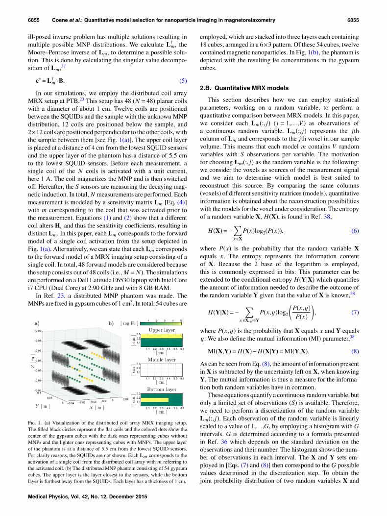
In our simulations, we employ the distributed coil arrayMRX setup at PTB.23 This setup has 48 (N = 48) planar coilswith a diameter of about 1 cm. Twelve coils are positionedbetween the SQUIDs and the sample with the unknown MNPdistribution, 12 coils are positioned below the sample, and2×12 coils are positioned perpendicular to the other coils, withthe sample between them [see Fig. 1(a)]. The upper coil layeris placed at a distance of 4 cm from the lowest SQUID sensorsand the upper layer of the phantom has a distance of 5.5 cmto the lowest SQUID sensors. Before each measurement, asingle coil of the N coils is activated with a unit current,here 1 A. The coil magnetizes the MNP and is then switchedoff. Hereafter, the S sensors are measuring the decaying mag-netic induction. In total, N measurements are performed. Eachmeasurement is modeled by a sensitivity matrix Lm [Eq. (4)]with m corresponding to the coil that was activated prior tothe measurement. Equations (1) and (2) show that a differentcoil alters Hv and thus the sensitivity coefficients, resulting indistinct Lm. In this paper, each Lm corresponds to the forwardmodel of a single coil activation from the setup depicted inFig. 1(a). Alternatively, we can state that each Lm correspondsto the forward model of a MRX imaging setup consisting of asingle coil. In total, 48 forward models are considered becausethe setup consists out of 48 coils (i.e., M = N). The simulationsare performed on a Dell Latitude E6530 laptop with Intel Corei7 CPU (Dual Core) at 2.90 GHz and with 8 GB RAM.

In Ref. 23, a distributed MNP phantom was made. TheMNPs are fixed in gypsum cubes of 1 cm3. In total, 54 cubes are

F. 1. (a) Visualization of the distributed coil array MRX imaging setup.The filled black circles represent the flat coils and the colored dots show thecenter of the gypsum cubes with the dark ones representing cubes withoutMNPs and the lighter ones representing cubes with MNPs. The upper layerof the phantom is at a distance of 5.5 cm from the lowest SQUID sensors.For clarity reasons, the SQUIDs are not shown. Each Lm corresponds to theactivation of a single coil from the distributed coil array with m referring tothe activated coil. (b) The distributed MNP phantom consisting of 54 gypsumcubes. The upper layer is the layer closest to the sensors, while the bottomlayer is furthest away from the SQUIDs. Each layer has a thickness of 1 cm.

employed, which are stacked into three layers each containing18 cubes, arranged in a 6×3 pattern. Of these 54 cubes, twelvecontained magnetic nanoparticles. In Fig. 1(b), the phantom isdepicted with the resulting Fe concentrations in the gypsumcubes.

2.B. Quantitative MRX models

This section describes how we can employ statisticalparameters, working on a random variable, to perform aquantitative comparison between MRX models. In this paper,we consider each Lm(:, j) ( j = 1,. . .,V ) as observations ofa continuous random variable. Lm(:, j) represents the jthcolumn of Lm and corresponds to the jth voxel in our samplevolume. This means that each model m contains V randomvariables with S observations per variable. The motivationfor choosing Lm(:, j) as the random variable is the following:we consider the voxels as sources of the measurement signaland we aim to determine which model is best suited toreconstruct this source. By comparing the same columns(voxels) of different sensitivity matrices (models), quantitativeinformation is obtained about the reconstruction possibilitieswith the models for the voxel under consideration. The entropyof a random variable X, H(X), is found in Ref. 38,

H(X)=−x∈X

P(x)log2(P(x)), (6)

where P(x) is the probability that the random variable Xequals x. The entropy represents the information contentof X. Because the 2 base of the logarithm is employed,this is commonly expressed in bits. This parameter can beextended to the conditional entropy H(Y|X) which quantifiesthe amount of information needed to describe the outcome ofthe random variable Y given that the value of X is known,38

H(Y|X)=−

x∈X, y∈YP(x,y)log2

(P(x,y)P(x)

), (7)

where P(x,y) is the probability that X equals x and Y equalsy . We also define the mutual information (MI) parameter,38

MI(X,Y)=H(X)−H(X|Y)=MI(Y,X). (8)

As can be seen from Eq. (8), the amount of information presentin X is subtracted by the uncertainty left on X, when knowingY. The mutual information is thus a measure for the informa-tion both random variables have in common.

These equations quantify a continuous random variable, butonly a limited set of observations (S) is available. Therefore,we need to perform a discretization of the random variableLm(:, j). Each observation of the random variable is linearlyscaled to a value of 1,. . .,G, by employing a histogram with Gintervals. G is determined according to a formula presentedin Ref. 36 which depends on the standard deviation on theobservations and their number. The histogram shows the num-ber of observations in each interval. The X and Y sets em-ployed in [Eqs. (7) and (8)] then correspond to the G possiblevalues determined in the discretization step. To obtain thejoint probability distribution of two random variables X and

Medical Physics, Vol. 42, No. 12, December 2015

6856 Coene et al.: Quantitative model selection for nanoparticle imaging in magnetorelaxometry 6856

Y (P(x,y),x ∈ X,y ∈ Y) [see Eqs. (7) and (8)], a joint histo-gram is made which is then divided by the total number ofoccurrences. The marginal distributions [P(x),x ∈X and P(y),y ∈Y] [Eqs. (7) and (8)] are calculated by

P(x)=y∈Y

P(x,y), P(y)=x∈X

P(x,y). (9)

2.C. Local weighting of quantitative MRX models

This section describes the transformation of Lm. The trans-formation uses the quantitative information from Eqs. (6)–(8).Based on this information, the transformation gives a weightto each column of Lm depending on its performances foreach voxel with respect to the other sensitivity matrices. Thetransformation is based on the approach described in Ref. 36,where EEG and MEG data were combined. Due to the natureof the inverse problem, some modifications of this methodwere necessary to be able to compare different Lm.

The complete transformation of Lm is mathematically ex-pressed as

T(Lm)=Nm ·Lm ·Wm ·Dm, (10)

where T(Lm) is called the transformed sensitivity matrix offorward model m and Lm the sensitivity matrix of forwardmodel m [Eq. (4), Sec. 2.A]. We will now detail all the differentsteps of this transformation. Figure 2 depicts an overview ofthe considered transformation.

Nm is a diagonal matrix and performs the normalization ofthe sensitivity matrix’s rows, so that a similar sensor signalis obtained for each model. Each element i on its diagonal is

F. 2. Method for quantitative comparison between different MRX forwardmodels using information theory parameters. Based on these parameters,a selective weighting of the forward models is possible. The weightingcoefficients give quantitative information about the efficiency of each modelwith respect to the voxels and allow a quantitative comparison between themodels.

calculated as follows: ∥Lm(i,:)∥−1 with Lm(i,:) (i = 1,. . .,S) theith row of Lm. Wm is a diagonal matrix with weights based onthe performance of the model for each voxel j in comparisonto the other M − 1 models. Dm is a diagonal matrix whichremoves the impact of source orientation and each element jon the diagonal is computed like this, ∥(Nm ·Lm ·Wm)(:, j)∥−1

with the operator (:, j) working on the resulting matrix fromthe multiplication of Nm ·Lm ·Wm.

Wm is determined by evaluating the conditional entropy[Eq. (7)] and mutual information [Eq. (8)] for sensitivitymatrix m compared to the other M − 1 sensitivity matricesfor each voxel j. To explain how the weighting works, wegive an example of two forward models with Lm with m = kand m = i which are compared to each other for the voxelj. It is beneficial to use the model that results in the lowestamount of uncertainty left, i.e., the model that gives the largestamount of information about the voxel j to be reconstructed. IfH(Lm=i(:, j)|Lm=k(:, j)) < H(Lm=k(:, j)|Lm=i(:, j)), this meansthe model with Lm=k is best suited to reconstruct the jth voxel.The jth column of Lm=k then receives a weighting of 1, whilethe jth column of Lm=i is given a weighting <1, determinedby minimization of the MI parameter [Eq. (8)]. This parameterrepresents the information both models have in common whenreconstructing voxel j. We choose the weighting for the jthcolumn of Lm=i such that the MI parameter is minimal,to reduce the amount of mutual information and this wayreduce the linearly dependent information. It has been shownpreviously in Ref. 24 that linearly dependent information candeteriorate the solution of the inverse problem. The use of theconditional entropy and MI parameters limits the comparisonto only two models at a time. To obtain the final weightingvalues for forward model k for voxel j, we repeat previouscomparison for the other remaining forward models (withm different from k and i). In total we will thus have M − 1weightings originating from the comparison of forward modelk to the other M−1 forward models. These M−1 weightingsare averaged to obtain the final weighting value for voxel j(Wm=k(:, j)). This can be done for each forward model. Themodels with the largest weightings on the jth column are thenmost favorable for reconstructing the MNP amount in voxel j.Remark that for significantly different weightings, informationmight be lost by averaging the weightings. For the modelsconsidered in this study, this is not the case, but this mightbecome a challenge for significantly different models or whenmany forward models are compared.

To compare the transformed sensitivity matrices to the orig-inal sensitivity matrices, we concatenate the M sensitivitymatrices into 1 matrix of dimensions (MS)×V defined as L forthe original sensitivity matrices and T(L) for the transformedsensitivity matrices,

T(L)=

T(L1)...

T(Lm)...

T(LM)

, (11)

Medical Physics, Vol. 42, No. 12, December 2015

6857 Coene et al.: Quantitative model selection for nanoparticle imaging in magnetorelaxometry 6857

with a similar definition for L. The forward model [Eq. (4)]and inverse problem [Eq. (5)] of T(L) become

T(B)=T(L) ·c, (12)

c∗=T(L)† ·T(B). (13)

Remark that the sensor signals generated with the forwardmodel now differ from the measured ones. This is because eachcolumn of the transformed sensitivity matrix is multiplied withweightings which are not in accordance with the sensitivitymatrices calculated from physical laws [Eqs. (1), (2), and (4)].Furthermore, this transformation of the sensitivity matrix isnonlinear due to the different weightings acting on each col-umn of the transformed sensitivity matrix. There exist multipleapproaches to solve this discrepancy: in Ref. 36, an itera-tive method, based on a rewriting of Eq. (4), was presentedto allow the use of measurement data and the transformedsensitivity matrix. Here, we look at the sensitivity coefficientsto determine the currents in the coils needed to realize T(B)experimentally. By taking the sum of the absolute values ofcolumn j from the sensitivity matrix, we have a measure forthe contribution of a signal, originating from voxel j, to thesensors, called the spatial sensitivity (T/mg) of voxel j,

ST(L)( j)=MSs=1

∥T(L)(s, j)∥ . (14)

By calculating ST(L), we can determine the required coil cur-rents in order to bring the measured B in correspondence withT(B). This approach allows to solve the inverse problem ina direct, noniterative, way. The spatial sensitivity is linearlyrelated to the current in the coils,31

ST(L)=A · I, (15)

where I is a N ×1 vector with the currents (A) for the N coilsand A is an interaction matrix [T/(mg A)] with dimensionsV × N . A depends on setup geometries and can be foundbased on a reformulation of the sensitivity coefficients in whichwe separate the I term from the sensitivity coefficients, Lm

= αmIcoil [Eqs. (1)–(3)]. Using Eqs. (4), (10), (11), and (14),we can then relate the current with the spatial sensitivity. Thecoil currents can then be determined as31

I∗=A† ·ST(L). (16)

One drawback of using the spatial sensitivity for determiningthe current in the coils is that in some cases, unrealistic currentscan be found for generating T(L). These currents cannot begenerated experimentally or would generate too large mag-netic fields that could damage the SQUID sensors. A thirdpossibility is to calculate the ratio between T(B) and B inthe forward model and to use these values for multiplying themeasured B. This might however amplify the noise present inthe measurement, which will in turn decrease the reconstruc-tion quality of the MNP distribution.

2.D. Measures for reconstruction quality

The spatial sensitivity [Eq. (14)] is an important measurein MRX imaging. Traditionally, it is high for voxels close to

the magnetizing coils and sensors and low for voxels furtheraway. A disadvantage of this quantity is that when the voxel isin close proximity to a sensor or coil, a large value is generatedwhile the contribution of the other (smaller) elements in thesummation do not matter anymore. This is why we employH(Y|X) [Eq. (7)] in order to include the spread on the sensi-tivity coefficients as an imaging parameter. We also employthe correlation coefficient (CC),31,32,35 which is a measure ofthe correspondence between the actual MNP distribution cand the reconstructed distribution c∗ [Eq. (5)]. A CC of 100%corresponds to a “perfect reconstruction.” Another quantity isthe condition number. This number indicates the stability of theinverse solution and is the ratio of the largest eigenvalue of thesensitivity matrix to the smallest eigenvalue of the sensitivitymatrix. This number should be as low as possible and directlyreflects how the solution (reconstruction) deteriorates whennoise is added. Very often, also the distribution of all eigen-values is compared to assess the impact of noise. In this paper,we verify our results using these established quantificationmethods.

3. RESULTS AND DISCUSSION3.A. Impact transformation on spatialand noise sensitivity

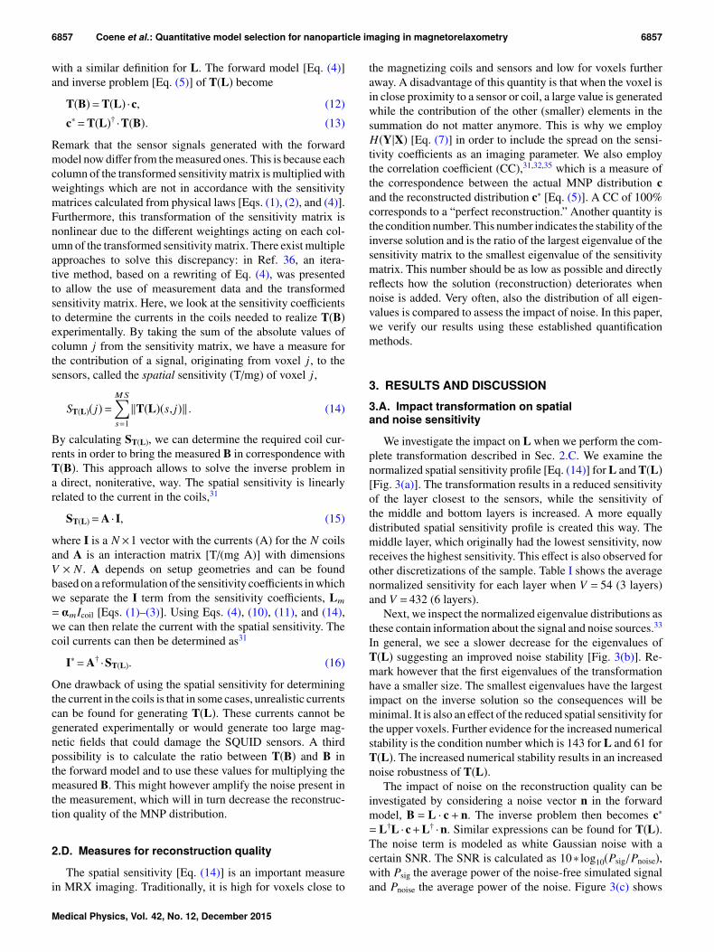
We investigate the impact on L when we perform the com-plete transformation described in Sec. 2.C. We examine thenormalized spatial sensitivity profile [Eq. (14)] for L and T(L)[Fig. 3(a)]. The transformation results in a reduced sensitivityof the layer closest to the sensors, while the sensitivity ofthe middle and bottom layers is increased. A more equallydistributed spatial sensitivity profile is created this way. Themiddle layer, which originally had the lowest sensitivity, nowreceives the highest sensitivity. This effect is also observed forother discretizations of the sample. Table I shows the averagenormalized sensitivity for each layer when V = 54 (3 layers)and V = 432 (6 layers).

Next, we inspect the normalized eigenvalue distributions asthese contain information about the signal and noise sources.33

In general, we see a slower decrease for the eigenvalues ofT(L) suggesting an improved noise stability [Fig. 3(b)]. Re-mark however that the first eigenvalues of the transformationhave a smaller size. The smallest eigenvalues have the largestimpact on the inverse solution so the consequences will beminimal. It is also an effect of the reduced spatial sensitivity forthe upper voxels. Further evidence for the increased numericalstability is the condition number which is 143 for L and 61 forT(L). The increased numerical stability results in an increasednoise robustness of T(L).

The impact of noise on the reconstruction quality can beinvestigated by considering a noise vector n in the forwardmodel, B = L · c+ n. The inverse problem then becomes c∗=L†L · c+L† ·n. Similar expressions can be found for T(L).The noise term is modeled as white Gaussian noise with acertain SNR. The SNR is calculated as 10∗ log10(Psig/Pnoise),with Psig the average power of the noise-free simulated signaland Pnoise the average power of the noise. Figure 3(c) shows

Medical Physics, Vol. 42, No. 12, December 2015

6858 Coene et al.: Quantitative model selection for nanoparticle imaging in magnetorelaxometry 6858

F. 3. (a) Normalized spatial sensitivity profile of L and T(L). T(L) shows a homogeneous sensitivity profile responsible for increased reconstruction qualitycompared to L. (b) The normalized eigenvalue distribution for L and T(L) shows an increased numerical stability for T(L). (c) Reconstruction of the PTBphantom for L and T(L) using simulated white Gaussian noise of 20 dB. Lower sources are shifted upward and are less accurately reconstructed when L isemployed due to the inherent lower sensitivity of these layers and the decreased numerical stability of this matrix.

the reconstruction of the PTB phantom for L and T(L) fornoise with a SNR of 20 dB (a commonly employed noiselevel, see Refs. 24 and 25). The associated CC’s are 95.5%and 99.8%, respectively. The difference is most striking for

T I. Normalized average spatial sensitivity for each layer for V = 54and V = 432 using L and T(L). The transformation realizes a homogeneoussensitivity which results in a higher sensitivity for lower layers and a lowersensitivity for the layer closest to the sensors.

V = 54 V = 432

Average sensitivity (−) L T(L) L T(L)

Upper layer(s) 0.82 0.600.77 0.490.52 0.65

Middle layer(s) 0.48 0.720.39 0.730.34 0.68

Bottom layer(s) 0.47 0.530.34 0.570.39 0.43

the middle layer where we find a correlation of 82.5% for Land 99.2% for T(L). Using L, lower-lying sources are liftedupward due to the decreased spatial sensitivity for the lowervoxels. For other noise levels (ranging from 1 to 40 dB), T(L)also outperforms L. Remark that the way of modeling the noisein simulated measurements has a significant impact on thereconstruction quality obtained in the simulations24 but cangive an indication of the performance of T(L). Although Land T(L) were investigated with a similar noise profile, weshould validate the transformation approach experimentally inthe future. Note that the impact of a double transformation,T(T(L)), is only marginal (≈1%) compared to T(L) which iswhy it is not considered.

3.B. Quantitative information

In this section, we consider two examples in which wedirectly use the quantitative information associated with theMRX models in order to enhance the MRX imaging setup. Ina first example, we want to find a reduced number of coils for

Medical Physics, Vol. 42, No. 12, December 2015

6859 Coene et al.: Quantitative model selection for nanoparticle imaging in magnetorelaxometry 6859

the setup by selecting a subset of coils based on their mutualinformation. In a second example, we determine an optimalvoxel size for the setup based on the information content ofthe statistical parameters.

3.B.1. Determining coil configuration

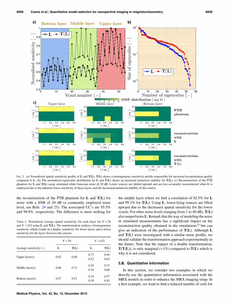
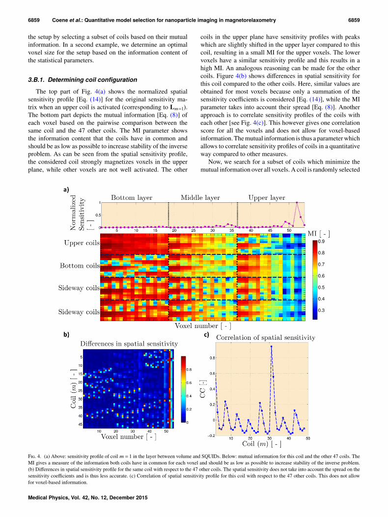
The top part of Fig. 4(a) shows the normalized spatialsensitivity profile [Eq. (14)] for the original sensitivity ma-trix when an upper coil is activated (corresponding to Lm=1).The bottom part depicts the mutual information [Eq. (8)] ofeach voxel based on the pairwise comparison between thesame coil and the 47 other coils. The MI parameter showsthe information content that the coils have in common andshould be as low as possible to increase stability of the inverseproblem. As can be seen from the spatial sensitivity profile,the considered coil strongly magnetizes voxels in the upperplane, while other voxels are not well activated. The other

coils in the upper plane have sensitivity profiles with peakswhich are slightly shifted in the upper layer compared to thiscoil, resulting in a small MI for the upper voxels. The lowervoxels have a similar sensitivity profile and this results in ahigh MI. An analogous reasoning can be made for the othercoils. Figure 4(b) shows differences in spatial sensitivity forthis coil compared to the other coils. Here, similar values areobtained for most voxels because only a summation of thesensitivity coefficients is considered [Eq. (14)], while the MIparameter takes into account their spread [Eq. (8)]. Anotherapproach is to correlate sensitivity profiles of the coils witheach other [see Fig. 4(c)]. This however gives one correlationscore for all the voxels and does not allow for voxel-basedinformation. The mutual information is thus a parameter whichallows to correlate sensitivity profiles of coils in a quantitativeway compared to other measures.

Now, we search for a subset of coils which minimize themutual information over all voxels. A coil is randomly selected

F. 4. (a) Above: sensitivity profile of coil m = 1 in the layer between volume and SQUIDs. Below: mutual information for this coil and the other 47 coils. TheMI gives a measure of the information both coils have in common for each voxel and should be as low as possible to increase stability of the inverse problem.(b) Differences in spatial sensitivity profile for the same coil with respect to the 47 other coils. The spatial sensitivity does not take into account the spread on thesensitivity coefficients and is thus less accurate. (c) Correlation of spatial sensitivity profile for this coil with respect to the 47 other coils. This does not allowfor voxel-based information.

Medical Physics, Vol. 42, No. 12, December 2015

6860 Coene et al.: Quantitative model selection for nanoparticle imaging in magnetorelaxometry 6860

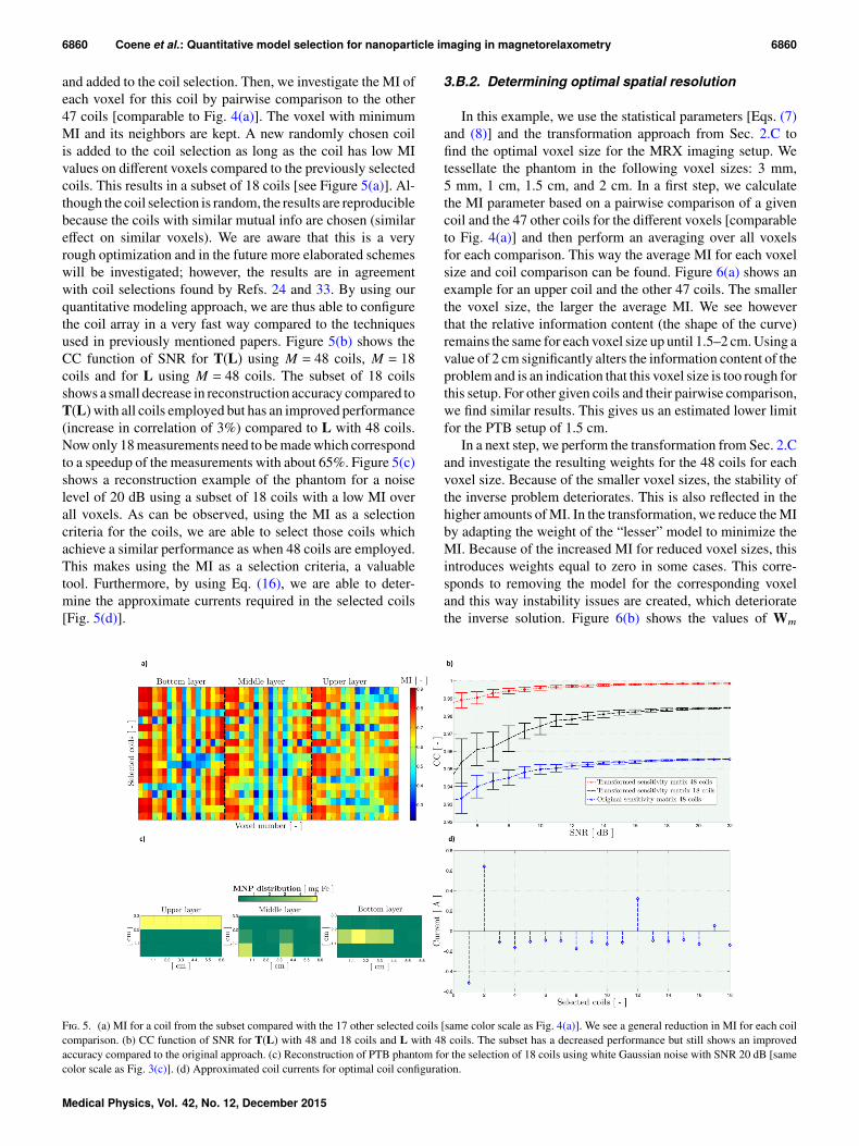
and added to the coil selection. Then, we investigate the MI ofeach voxel for this coil by pairwise comparison to the other47 coils [comparable to Fig. 4(a)]. The voxel with minimumMI and its neighbors are kept. A new randomly chosen coilis added to the coil selection as long as the coil has low MIvalues on different voxels compared to the previously selectedcoils. This results in a subset of 18 coils [see Figure 5(a)]. Al-though the coil selection is random, the results are reproduciblebecause the coils with similar mutual info are chosen (similareffect on similar voxels). We are aware that this is a veryrough optimization and in the future more elaborated schemeswill be investigated; however, the results are in agreementwith coil selections found by Refs. 24 and 33. By using ourquantitative modeling approach, we are thus able to configurethe coil array in a very fast way compared to the techniquesused in previously mentioned papers. Figure 5(b) shows theCC function of SNR for T(L) using M = 48 coils, M = 18coils and for L using M = 48 coils. The subset of 18 coilsshows a small decrease in reconstruction accuracy compared toT(L)with all coils employed but has an improved performance(increase in correlation of 3%) compared to L with 48 coils.Now only 18 measurements need to be made which correspondto a speedup of the measurements with about 65%. Figure 5(c)shows a reconstruction example of the phantom for a noiselevel of 20 dB using a subset of 18 coils with a low MI overall voxels. As can be observed, using the MI as a selectioncriteria for the coils, we are able to select those coils whichachieve a similar performance as when 48 coils are employed.This makes using the MI as a selection criteria, a valuabletool. Furthermore, by using Eq. (16), we are able to deter-mine the approximate currents required in the selected coils[Fig. 5(d)].

3.B.2. Determining optimal spatial resolution

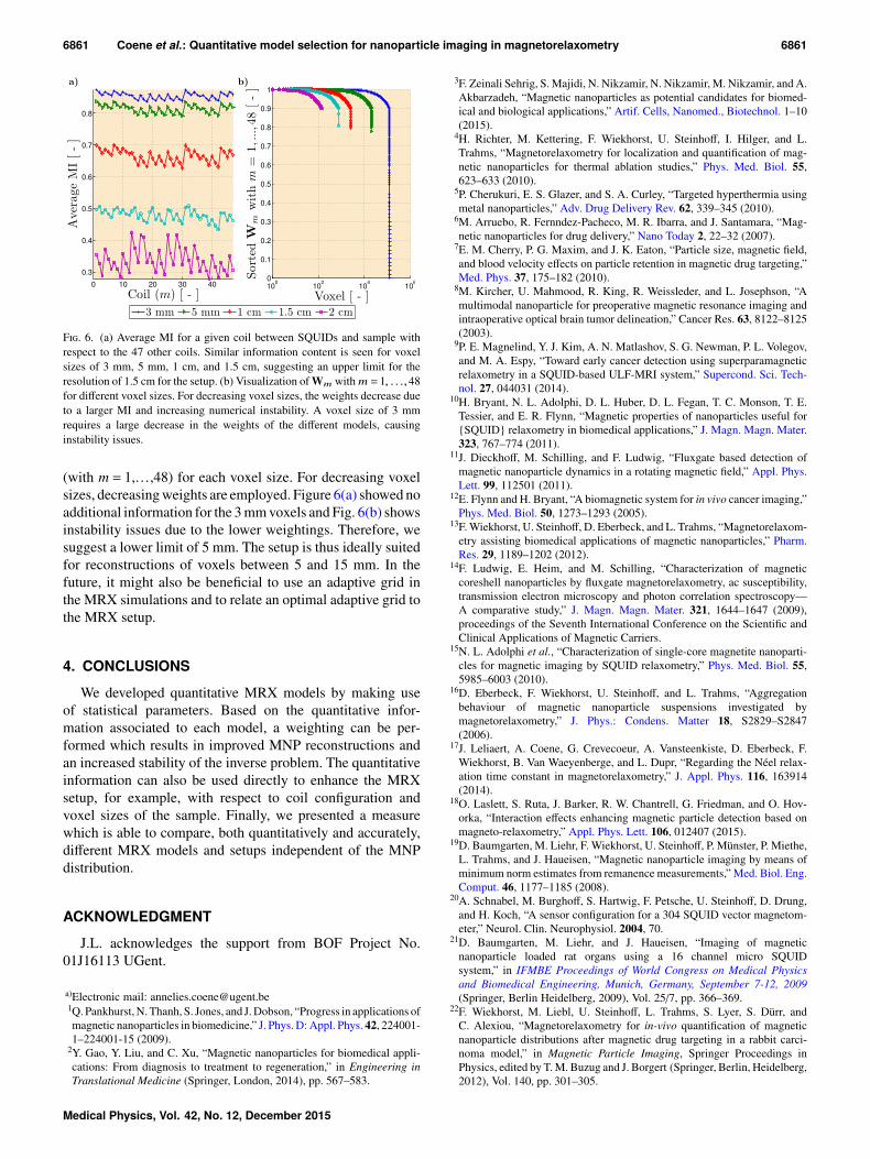
In this example, we use the statistical parameters [Eqs. (7)and (8)] and the transformation approach from Sec. 2.C tofind the optimal voxel size for the MRX imaging setup. Wetessellate the phantom in the following voxel sizes: 3 mm,5 mm, 1 cm, 1.5 cm, and 2 cm. In a first step, we calculatethe MI parameter based on a pairwise comparison of a givencoil and the 47 other coils for the different voxels [comparableto Fig. 4(a)] and then perform an averaging over all voxelsfor each comparison. This way the average MI for each voxelsize and coil comparison can be found. Figure 6(a) shows anexample for an upper coil and the other 47 coils. The smallerthe voxel size, the larger the average MI. We see howeverthat the relative information content (the shape of the curve)remains the same for each voxel size up until 1.5–2 cm. Using avalue of 2 cm significantly alters the information content of theproblem and is an indication that this voxel size is too rough forthis setup. For other given coils and their pairwise comparison,we find similar results. This gives us an estimated lower limitfor the PTB setup of 1.5 cm.

In a next step, we perform the transformation from Sec. 2.Cand investigate the resulting weights for the 48 coils for eachvoxel size. Because of the smaller voxel sizes, the stability ofthe inverse problem deteriorates. This is also reflected in thehigher amounts of MI. In the transformation, we reduce the MIby adapting the weight of the “lesser” model to minimize theMI. Because of the increased MI for reduced voxel sizes, thisintroduces weights equal to zero in some cases. This corre-sponds to removing the model for the corresponding voxeland this way instability issues are created, which deterioratethe inverse solution. Figure 6(b) shows the values of Wm

F. 5. (a) MI for a coil from the subset compared with the 17 other selected coils [same color scale as Fig. 4(a)]. We see a general reduction in MI for each coilcomparison. (b) CC function of SNR for T(L) with 48 and 18 coils and L with 48 coils. The subset has a decreased performance but still shows an improvedaccuracy compared to the original approach. (c) Reconstruction of PTB phantom for the selection of 18 coils using white Gaussian noise with SNR 20 dB [samecolor scale as Fig. 3(c)]. (d) Approximated coil currents for optimal coil configuration.

Medical Physics, Vol. 42, No. 12, December 2015

6861 Coene et al.: Quantitative model selection for nanoparticle imaging in magnetorelaxometry 6861

F. 6. (a) Average MI for a given coil between SQUIDs and sample withrespect to the 47 other coils. Similar information content is seen for voxelsizes of 3 mm, 5 mm, 1 cm, and 1.5 cm, suggesting an upper limit for theresolution of 1.5 cm for the setup. (b) Visualization of Wm with m = 1, . . .,48for different voxel sizes. For decreasing voxel sizes, the weights decrease dueto a larger MI and increasing numerical instability. A voxel size of 3 mmrequires a large decrease in the weights of the different models, causinginstability issues.

(with m = 1,. . .,48) for each voxel size. For decreasing voxelsizes, decreasing weights are employed. Figure 6(a) showed noadditional information for the 3 mm voxels and Fig. 6(b) showsinstability issues due to the lower weightings. Therefore, wesuggest a lower limit of 5 mm. The setup is thus ideally suitedfor reconstructions of voxels between 5 and 15 mm. In thefuture, it might also be beneficial to use an adaptive grid inthe MRX simulations and to relate an optimal adaptive grid tothe MRX setup.

4. CONCLUSIONS

We developed quantitative MRX models by making useof statistical parameters. Based on the quantitative infor-mation associated to each model, a weighting can be per-formed which results in improved MNP reconstructions andan increased stability of the inverse problem. The quantitativeinformation can also be used directly to enhance the MRXsetup, for example, with respect to coil configuration andvoxel sizes of the sample. Finally, we presented a measurewhich is able to compare, both quantitatively and accurately,different MRX models and setups independent of the MNPdistribution.

ACKNOWLEDGMENT

J.L. acknowledges the support from BOF Project No.01J16113 UGent.

a)Electronic mail: annelies.coene@ugent.be1Q. Pankhurst, N. Thanh, S. Jones, and J. Dobson, “Progress in applications ofmagnetic nanoparticles in biomedicine,” J. Phys. D: Appl. Phys. 42, 224001-1–224001-15 (2009).

2Y. Gao, Y. Liu, and C. Xu, “Magnetic nanoparticles for biomedical appli-cations: From diagnosis to treatment to regeneration,” in Engineering inTranslational Medicine (Springer, London, 2014), pp. 567–583.

3F. Zeinali Sehrig, S. Majidi, N. Nikzamir, N. Nikzamir, M. Nikzamir, and A.Akbarzadeh, “Magnetic nanoparticles as potential candidates for biomed-ical and biological applications,” Artif. Cells, Nanomed., Biotechnol. 1–10(2015).

4H. Richter, M. Kettering, F. Wiekhorst, U. Steinhoff, I. Hilger, and L.Trahms, “Magnetorelaxometry for localization and quantification of mag-netic nanoparticles for thermal ablation studies,” Phys. Med. Biol. 55,623–633 (2010).

5P. Cherukuri, E. S. Glazer, and S. A. Curley, “Targeted hyperthermia usingmetal nanoparticles,” Adv. Drug Delivery Rev. 62, 339–345 (2010).

6M. Arruebo, R. Fernndez-Pacheco, M. R. Ibarra, and J. Santamara, “Mag-netic nanoparticles for drug delivery,” Nano Today 2, 22–32 (2007).

7E. M. Cherry, P. G. Maxim, and J. K. Eaton, “Particle size, magnetic field,and blood velocity effects on particle retention in magnetic drug targeting,”Med. Phys. 37, 175–182 (2010).

8M. Kircher, U. Mahmood, R. King, R. Weissleder, and L. Josephson, “Amultimodal nanoparticle for preoperative magnetic resonance imaging andintraoperative optical brain tumor delineation,” Cancer Res. 63, 8122–8125(2003).

9P. E. Magnelind, Y. J. Kim, A. N. Matlashov, S. G. Newman, P. L. Volegov,and M. A. Espy, “Toward early cancer detection using superparamagneticrelaxometry in a SQUID-based ULF-MRI system,” Supercond. Sci. Tech-nol. 27, 044031 (2014).

10H. Bryant, N. L. Adolphi, D. L. Huber, D. L. Fegan, T. C. Monson, T. E.Tessier, and E. R. Flynn, “Magnetic properties of nanoparticles useful for{SQUID} relaxometry in biomedical applications,” J. Magn. Magn. Mater.323, 767–774 (2011).

11J. Dieckhoff, M. Schilling, and F. Ludwig, “Fluxgate based detection ofmagnetic nanoparticle dynamics in a rotating magnetic field,” Appl. Phys.Lett. 99, 112501 (2011).

12E. Flynn and H. Bryant, “A biomagnetic system for in vivo cancer imaging,”Phys. Med. Biol. 50, 1273–1293 (2005).

13F. Wiekhorst, U. Steinhoff, D. Eberbeck, and L. Trahms, “Magnetorelaxom-etry assisting biomedical applications of magnetic nanoparticles,” Pharm.Res. 29, 1189–1202 (2012).

14F. Ludwig, E. Heim, and M. Schilling, “Characterization of magneticcoreshell nanoparticles by fluxgate magnetorelaxometry, ac susceptibility,transmission electron microscopy and photon correlation spectroscopy—A comparative study,” J. Magn. Magn. Mater. 321, 1644–1647 (2009),proceedings of the Seventh International Conference on the Scientific andClinical Applications of Magnetic Carriers.

15N. L. Adolphi et al., “Characterization of single-core magnetite nanoparti-cles for magnetic imaging by SQUID relaxometry,” Phys. Med. Biol. 55,5985–6003 (2010).

16D. Eberbeck, F. Wiekhorst, U. Steinhoff, and L. Trahms, “Aggregationbehaviour of magnetic nanoparticle suspensions investigated bymagnetorelaxometry,” J. Phys.: Condens. Matter 18, S2829–S2847(2006).

17J. Leliaert, A. Coene, G. Crevecoeur, A. Vansteenkiste, D. Eberbeck, F.Wiekhorst, B. Van Waeyenberge, and L. Dupr, “Regarding the Néel relax-ation time constant in magnetorelaxometry,” J. Appl. Phys. 116, 163914(2014).

18O. Laslett, S. Ruta, J. Barker, R. W. Chantrell, G. Friedman, and O. Hov-orka, “Interaction effects enhancing magnetic particle detection based onmagneto-relaxometry,” Appl. Phys. Lett. 106, 012407 (2015).

19D. Baumgarten, M. Liehr, F. Wiekhorst, U. Steinhoff, P. Münster, P. Miethe,L. Trahms, and J. Haueisen, “Magnetic nanoparticle imaging by means ofminimum norm estimates from remanence measurements,” Med. Biol. Eng.Comput. 46, 1177–1185 (2008).

20A. Schnabel, M. Burghoff, S. Hartwig, F. Petsche, U. Steinhoff, D. Drung,and H. Koch, “A sensor configuration for a 304 SQUID vector magnetom-eter,” Neurol. Clin. Neurophysiol. 2004, 70.

21D. Baumgarten, M. Liehr, and J. Haueisen, “Imaging of magneticnanoparticle loaded rat organs using a 16 channel micro SQUIDsystem,” in IFMBE Proceedings of World Congress on Medical Physicsand Biomedical Engineering, Munich, Germany, September 7-12, 2009(Springer, Berlin Heidelberg, 2009), Vol. 25/7, pp. 366–369.

22F. Wiekhorst, M. Liebl, U. Steinhoff, L. Trahms, S. Lyer, S. Dürr, andC. Alexiou, “Magnetorelaxometry for in-vivo quantification of magneticnanoparticle distributions after magnetic drug targeting in a rabbit carci-noma model,” in Magnetic Particle Imaging, Springer Proceedings inPhysics, edited by T. M. Buzug and J. Borgert (Springer, Berlin, Heidelberg,2012), Vol. 140, pp. 301–305.

Medical Physics, Vol. 42, No. 12, December 2015

6862 Coene et al.: Quantitative model selection for nanoparticle imaging in magnetorelaxometry 6862

23M. Liebl, U. Steinhoff, F. Wiekhorst, J. Haueisen, and L. Trahms, “Quan-titative imaging of magnetic nanoparticles by magnetorelaxometry withmultiple excitation coils,” Phys. Med. Biol. 59, 6607–6620 (2014).

24A. Coene, G. Crevecoeur, M. Liebl, F. Wiekhorst, L. Dupré, and U.Steinhoff, “Uncertainty of reconstructions of spatially distributed magneticnanoparticles under realistic noise conditions,” J. Appl. Phys. 115, 17B509(2014).

25D. Baumgarten and J. Haueisen, “A spatio-temporal approach for the solu-tion of the inverse problem in the reconstruction of magnetic nanoparticledistributions,” IEEE Trans. Magn. 46, 3496–3499 (2010).

26M. Liebl, U. Steinhoff, F. Wiekhorst, A. Coene, J. Haueisen, and L.Trahms, “Quantitative reconstruction of a magnetic nanoparticle distribu-tion using a non-negativity constraint,” Biomed. Eng./Biomed. Tech. 58, 2(2013).

27R. Eichardt and J. Haueisen, “Influence of sensor variations on the condi-tion of the magnetostatic linear inverse problem,” IEEE Trans. Magn. 46,3449–3452 (2010).

28R. Eichardt, D. Baumgarten, B. Petkovic, F. Wiekhorst, L. Trahms, and J.Haueisen, “Adapting source grid parameters to improve the condition of themagnetostatic linear inverse problem of estimating nanoparticle distribu-tions,” Med. Biol. Eng. Comput. 50, 1081–1089 (2012).

29J. P. Wikswo, Y. Ma, N. Sepulveda, S. Tan, I. Thomas, and A. Lauder, “Mag-netic susceptibility imaging for nondestructive evaluation (using SQUIDmagnetometer),” IEEE Trans. Appl. Supercond. 3, 1995–2002 (1993).

30N. Sepulveda, I. Thomas, and J. P. Wikswo, “Magnetic susceptibility tomog-raphy for three-dimensional imaging of diamagnetic and paramagnetic ob-jects,” IEEE Trans. Magn. 30, 5062–5069 (1994).

31G. Crevecoeur, D. Baumgarten, U. Steinhoff, J. Haueisen, L. Thrams, andL. Dupré, “Advancements in magnetic nanoparticle reconstruction usingsequential activation of excitation coil arrays using magnetorelaxometry,”IEEE Trans. Magn. 48, 1313–1316 (2012).

32A. Coene, G. Crevecoeur, and L. Dupré, “Adaptive control of excitation coilarrays for targeted magnetic nanoparticle reconstruction using magnetore-laxometry,” IEEE Trans. Magn. 48, 2842–2845 (2012).

33D. Baumgarten, R. Eichardt, G. Crevecoeur, E. Supriyanto, and J.Haueisen, “Magnetic nanoparticle imaging by random and maximumlength sequences of inhomogeneous activation fields,” in 35th AnnualInternational Conference of the IEEE on Engineering in Medicine andBiology Society (EMBC) (IEEE, New York, NY, 2013), pp. 3258–3260.

34N. K. Hoo, M. Klemm, E. Supriyanto, and D. Baumgarten, “Effects ofexcitation coil configurations in magnetorelaxometry imaging of magneticnanoparticles,” in IEEE Conference on Biomedical Engineering andSciences (IECBES) (IEEE, New York, NY, 2014), pp. 715–718.

35D. Baumgarten, F. Braune, E. Supriyanto, and J. Haueisen, “Plane-wisesensitivity based inhomogeneous excitation fields for magnetorelaxometryimaging of magnetic nanoparticles,” J. Magn. Magn. Mater. 380, 255–260(2014).

36S. Baillet, L. Garnero, G. Marin, and J.-P. Hugonin, “Combined MEG andEEG source imaging by minimization of mutual information,” IEEE Trans.Biomed. Eng. 46, 522–534 (1999).

37P. Hansen, “The truncated SVD as a method for regularization,” BIT Numer.Math. 27, 534–553 (1987).

38C. E. Shannon, “A mathematical theory of communication,” Bell Syst. Tech.J. 27, 379–423 (1948).

Medical Physics, Vol. 42, No. 12, December 2015