36
1/25/2012 Quantitative Tools for Research KASHIF QADRI Descriptive Analysis Lecture Week 4 1

1/25/2012
Quantitative Tools for Research
KASHIF QADRI
Descriptive Analysis
Lecture Week 4
1

1/25/2012
Overview Measurement of Central Tendency / Location
Mean, Median & Mode
Quantiles (Quartiles, Deciles, Percentiles)
Measurement of Dispersion
Range & Quartile Deviation
Variance and Standard Deviation
The concept of outliers
3
Descriptive Analysis Describing the characteristics of the data
Revealing the distribution
Leading towards further analysis
Concluding on the basis descriptive analysis
4
2

1/25/2012
Measures of Central Tendency
Central Tendency
All the values in a data tend towards it center.
3

1/25/2012
Central Tendency The values, in a data set, tend towards a
central value that is called central tendency.
It summarizes a data set in a single value.
The methods to measure central tendency are
called Measures of “Central Tendency” , “Location”, “Position” or simply “Average”.
7
The Arithmetic Mean x
The Arithmetic Mean or Simply the mean is
the most widely used average. It is defined as
“the sum of the observations divided by the
number of the observations”. It is indicated by
AM or μ or x
8
4

1/25/2012
The Arithmetic Mean Mean = Sum of observations
No. of observations
Let the observations are x1, x2, x3,…, xn. Then the arithmetic mean (μ or ) will be:
x x
9
= x1 + x2 + x3 + … + xn = Σxi n n
μ = Population Mean
x = Sample Mean
Example Find the AM of: 4, 7, -2, 0 and 8.
Mean = ( 4 + 7 - 2 + 0 + 8 ) / 5
= 17 / 5
= 3.4 Ans.
10
5

1/25/2012
Weighted Mean
According the relative importance of numbers
their weights are assigned.
Hence weighted mean is obtained as:
WM = w1*x1 +w2*x2 + … + wk*xk
w1 + w2 + … + wk
WM = Σwx
11
Σw
Example
A student scored 45, 80 and 60 in three
quizzes. The weights of these quizzes are 1, 2
and 5 respectively. Find the weighted score of
this student.
12
6

1/25/2012
Solution Weighted Mean = w1*x1 + w2*x2 + w3*x3
w1 + w2 + w3
WM = 1* 45 + 2 * 80 + 5 * 60
1 + 2 + 5
WM = 505
8
Weighted Mean = 63.125
13
14
7

1/25/2012
Combined Mean The combined mean of k groups can be
obtained by:
CM = n1*m1 + n2*m2 + … + nk*mk
n1 + n2 + … + nk
CM = Σnm
Σn
15
Example The mean of three samples are given below. Find
the combined mean.
Sample #
No. of values
Mean
1
32
1158
2
17
1897
3
26
1453
16
8

1/25/2012
Solution CM = n1*m1 + n2*m2 + n3*m3
n1
+ n2 + n3
CM = 32 * 1158 + 17 * 1897 + 26 * 1453
32 + 17 + 26
= 37056 + 32249 + 37778
75
= 107083 / 75
Combined mean = 1427.77
17
Properties of Arithmetic Mean 1. The sum of deviations of all observations from AM is always zero. 2. The sum of square of deviations of each observation from AM is minimum. 3. Linear Transformation
4. Change of Origin & Scale
18
9

1/25/2012
Linear Transformation
If there is a linear relationship between two
variables X andY, i.e.
Y= a + bx where “a” & “b” are any constants
but a ≠ 0.
___
Then
y
= a + b x
19
Example The average salary of workers in a factory is $580. If their salary
is raised by 2% and a further bonus $50 is given to each, then find the new average salary. X = 580, a = 1.02 , b = 50 ; Y = ?
Formula: Mean of Y = a + b * Mean of x
= 50 + 1.02 * 580
= $641.6
20
10

1/25/2012
The Median Median is the value which divides the ordered data set into
two equal parts (or it is middle most observation in the
ordered data).
Data line:
Median
0%
50%
100%
27
Median Median is the middle most observation in
the arranged data.
Median divides the ordered data into two
halves.
50% values lie below median and 50%
above median.
28
Median
14

1/25/2012
For Odd number of observations Formula:
Median = (n + 1)th observation 2
Find the median of: 2, - 6, 0, 11, 7, 5, and - 1
Median = (n + 1) = (7 + 1) = 4th observation
2
2 Arranged data: - 6, - 1, 0, 2, 5, 7, 11
Median = 2
29
Question
Find the median of the following data:
17, -13, 21, 9, 0, -8, 13, 7, 2
Solution:
- 13, - 8, 0, 2, 7, 9, 13, 17, 21
Median = 7
30
15

1/25/2012
For Even number of observations Formula:
Median is AM of { n/2 & (n/2 + 1)}th obs.
Find the median of : 4, -6, 0, 7, 4, 2, -9, 10
Here n = 8 So median will be:
AM of ( 4th & 5th) observations i.e.
Ordered data: -9, -6, 0, 2, 4, 4, 7, 10
Median = (2 + 4)/2 = 3
31
Question
Find the median of the following data:
45, 10, 36, 28, 17, 32, 11, 37, 22, 41
Ordered Data:
10, 11, 17, 22, 28, 32, 36, 37, 41, 45
Median = (28 + 32)/2 = 30
32
16
1/25/2012
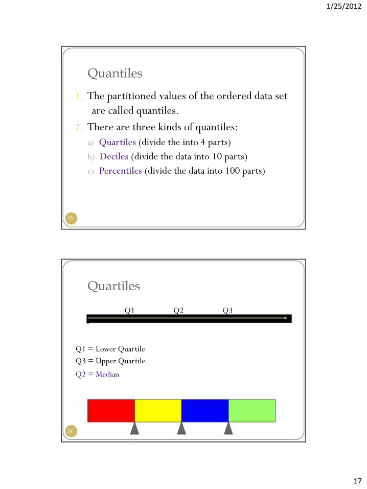
Quantiles
1. The partitioned values of the ordered data set
are called quantiles.
2. There are three kinds of quantiles:
a) Quartiles (divide the into 4 parts)
b) Deciles (divide the data into 10 parts)
c) Percentiles (divide the data into 100 parts)
33
Quartiles
Q1
Q2
Q3
Q1 = Lower Quartile
Q3 = Upper Quartile
Q2 = Median
34
17

1/25/2012
Quartiles
There are three quartiles Q1, Q2, and Q3.
Q1 is the value below which 25% data lies.
Q2 is the value below which 50% data lies.
Q3 is the value below which 75% data lies.
Q1 = (n +1)th obs. & Q3 = 3(n +1)th obs.
4
4
35
Example Find the lower and upper quartiles of the data given below.
4, 3, 9, 0, 1, 6, 8, 4, 3, 0, 2, 10, 13.
Arranging in ascending Order (n = 13):
0
0
1
2
3
3
4
4
6
8
9
10
13
36
18

1/25/2012
Solution Lower Quartile (Q1)
Q1 = (13+1)/4 = 3.5
= 4th Obs.
Q1 = 2
Upper Quartile (Q3)
Q3 = 3 (13 +1)/4 = 10.5 = 11th Obs.
Q3 = 9
37
Deciles
Deciles divide the ordered data set into TEN
parts.
D1 D2 … D5 …
D9
10
20
50
90
General Formula: Di = i*(n +1)/10
38
19

1/25/2012
Example Find 4th decile of the following series:
3,
6 ,
9, …,
884,
887,
900
4th Decile (D4):
Here n = 300 ( i.e. 300 observations ) D4 = 4(n +1)/10 value
D4 = 4(301)10 = 120.4 = 120 (round off)
Hence D4 will be 120th Obs. i.e. D4 = 360
39
Percentiles
P1
…
P50 …
P99
1 2
50%
99%
Partition the ordered data set into 100 parts.
General Formula: Pi = i*(n + 1)/100
40
20

1/25/2012
Example Find 78th percentile of the following series:
3,
6 ,
9, …,
884,
887,
900
78th Percentile
P78 = 78(n+1)/100
= 78(301)/100 = 234.78 = 235
P78 = 235th Observation.
P78 = 705
41
The Mode Mode is the most frequent observation in the data.
It is the value which is repeated largest number of times.
If two values are repeated same number of times both of them
will be mode.
If all the values are repeated equal number of times than there
will be no mode.
42
21

1/25/2012
Example Find the mode of:
a) 1, 2, 1, 3 2, 3, 0, 1, 4, 5, 2, 3, 3
Mode = 3
b) 2, 2, 1, 3, 5, 0, 5, 0, 0, 4, 1, 6, 1
Modes = 0 and 1
Why? (Both are repeated equal number of times)
c) 1, 2, 3, 5, 4, 7, 0, 6, 8, 9, 15
Mode: none
Why? (All values are once in the data.)
43
When to Use? Mean
Mean most generally used central tendency
Popular measure of central tendency because of it properties
Fails if observations are scattered or extreme values are there
Median
Strong measurement in ordered data
Good for qualitative ordered data
Has no affect of extreme values
Lacks mathematical properties
Mode
Helpful if the values are close and repeated
Lack mathematical treatment
44
22

1/25/2012
Measurement of Dispersion
Definition If the values in a data set are scattered apart
much than simply central tendency will not
describe the data adequately. Hence the
measure of spread is also applied to the data.
The additional information that measures the
scattered nature of a data set is called
dispersion.
23

1/25/2012
It is useful especially when two data sets are
to be compared. There are two types of
dispersion: absolute and relative.
The
dispersion is expressed in the units same as
the data.
The Range (R)
• Measure of Variation
• Difference Between Largest & Smallest
Observations:
Range =
xm x
0 • Ignores How Data Are Distributed:
Range = 12 - 7 = 5
Range = 12 - 7 = 5
7
8
9
10
11
12
7
8
9
10
11
12
24

1/25/2012
Formula
Range = Xm - Xo
Coefficient of Range =
Xm - X0
Xm + X0
Example Find Range and Coefficient of Range of: 2,
5,
6,
10,
-4,
-3, 0,
5, 11
Here: Xm = 11
Xo
= - 4 R = 11 - ( - 4) = 15
Co eff. of R = 11 - ( - 4 ) =
15
= 2.14 11 + ( - 4 )
7
25

Let us take two sets of observations. Set A contains marks of five students in Mathematics out of 25 marks and group B contains marks of the same student in English out of 100 marks. Set A: 10, 15, 18, 20, 20 Set B: 30, 35, 40, 45, 50 The values of range and coefficient of range are calculated as:
Range Coefficient of Range
Set A: (Mathematics)
20-10 =10 20-10/20+10=0.33
Set B: (English) 50-30 =20 50-30/50+30=0.25

1/25/2012
Quartile Deviation Quartile Deviation (QD) is the half of the
difference between upper and lower
quartile.
Quartile deviation is also called semi inter-
quartile range.
Formula
QD =
Q3 - Q1 2
26

1/25/2012
Example The students of a class scored the following marks in
a certain quiz. Find the quartile deviation and
coefficient of quartile deviation of marks.
40, 12, 27, 11, 5, 33, 45, 21, 37, & 43
Ordered data:
5, 11, 12, 21, 27, 33, 37, 40, 43, 45
Solution No. of observations = n = 10
Q1 = (n + 1)/4 = 11/4 = 2.75 3rd Obs. Q3 = 3(n + 1)/4 = 33/4 = 8.25 8th Obs.
So
Q1 = 12
Q3 = 40 QD = Q3 - Q1 = 40 - 12 = 14
2
2
27

1/25/2012
Variance
It is an important Measure of Variation. It
shows variation about the arithmetic mean.
•For the Population:
•For the Sample:
For the Population: use N in
For the Sample : use n - 1
the denominator.
in the denominator.
Standard Deviation
•Most Important Measure of Variation
•Shows Variation About the Mean:
•For the Population:
•For the Sample:
s
For the Population: use N in
the denominator.
2
Xi N
Xi X 2
n 1
For the Sample : use n - 1
in the denominator.
28
1/25/2012
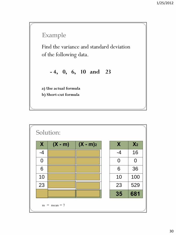
Example Find the variance and standard deviation
of the following data.
- 4,
0,
6,
10 and
23
a) Use actual formula b) Short-cut formula
Solution:
X
(X - m)
(X - m)2
X
X2
-4
-4
16 0
0
0 6
6
36 10
10
100 23
23
529
35
681
m = mean = 7
30

1/25/2012
Calculations Actual
m = ΣX/n = 35/5 = 7
S2 = Σ(X - m)2
n S2 = 436 / 5
S2 = 87.2
S = 9.3381
Solution:
X
X2
31

1/25/2012
Calculations
Actual
Short - Cut
X= ΣX/n = 35/5 = 7
S2 = ΣX2
- ( ΣX )2
S2 = (X - X)2
n
n n
S2 =
681
- ( 35 )2
S2 = 436 / 5
5
5 S2 = 87.2
S2 = 136.2 - ( 7 )2
S = 9.3381
S2 = 87.2 S = 9.3381
CoComparison of three data setseviations
Data A
Mean = 15.5 11 12 13 14 15
Data B
16 17 18 19 20 21 s
= 3.338
Mean = 15.5
11 12 13 14 15 16 17 18 19 20 21
Data C
11 12 13 14 15 16 17 18 19 20 21
s = .9258
Mean = 15.5
s = 4.57
32

1/25/2012
Coefficient of Variation
Example CV = SD x 100
Mean
CV =
9.3381 x 100
= 133.4 %
7
In comparing two data sets, the data set having less CV is considered more consistent.
33
Coefficient of Variation Measure of Relative Variation Always a % Shows Variation Relative to Mean Used to Compare 2 or More Groups Formula (for sample):

1/25/2012
Comparing CVs
Stock A: Average Price last year = $50
Standard Deviation = $5 Stock B: Average Price last year = $100
Standard Deviation = $5
Coefficient of Variation:
Stock A: CV = 10%
Stock B: CV = 5%
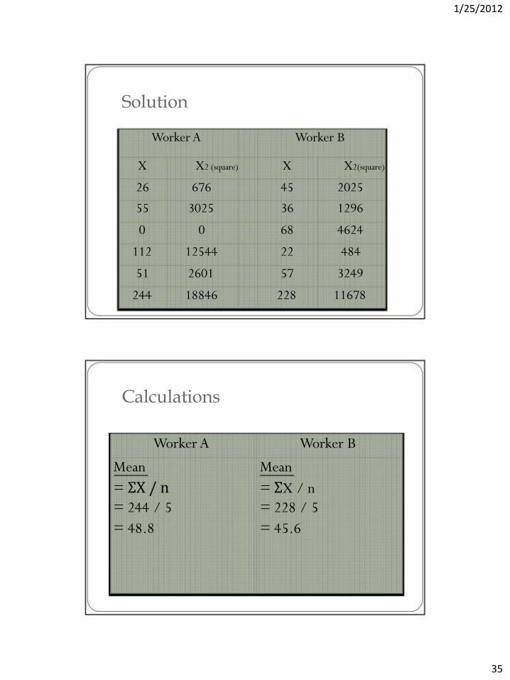
Example: The units produced by two worker in last week
are given below. Which worker is more consistent
in terms of production?
Day
Mon
Tue
Wed
Thu
Fri
Worker A
26
55
0
112
51
Worker B
45
36
68
22
57
34
1/25/2012
Solution
Worker A
Worker B
X
X2 (square)
X
X2(square)
26
676
45
2025
55
3025
36
1296
0
0
68
4624
112
12544
22
484
51
2601
57
3249
244
18846
228
11678
Calculations
Worker A
Worker B
Mean
Mean
= ΣX / n
= ΣX / n
= 244 / 5
= 228 / 5
= 48.8
= 45.6
35

1/25/2012
Worker A
Worker B
Variance
Variance
S2 = ΣX2 - ( ΣX )2
S2 = ΣX2 - ( ΣX )2
n
n
n
n
S2 = 18846 - (244)2
S2 = 11678 - (228)2
5
5
5
5
S2 =3769.5 -2381.44
S2 = 2335.6 -2079.36
S2 = 1388.06
S2 = 256.24
Worker A
Worker B
Standard Deviation
S = √1388.06 = 37.26
Co-eff. of Variance
CV = S * 100
X
CV = 37.26 * 100
48.8
CV = 76.35%
Standard Deviation
S = √256.24 = 16.01
Co-eff. of Variance
CV = S * 100
X
CV = 16.01 * 100
45.6
CV = 35.11%
36

1/25/2012
Summary of Results
Worker A
Worker B
Mean
48.8
45.6
Variance (S2)
1388.06
256.04
SD (S)
37.26
16.01
CV
76.35%
35.11%
Result: Here CVB < CVA hence worker B
is more consistent in his performance.
Inter Quartile Range IQR = Q3 - Q1
The quartiles of a data set are
Q1 = 25
Q3 = 38
Find IQR = 38 - 25 = 13
37

1/25/2012
Concept of Outlier Extreme values in a data set are called outliers
It is difficult to identify sometimes outlier especially when
the data is large
Our results are affected because of outliers
Hence we detect outliers and remove them and then perform
out anslysis
75
How to find outliers? Lower limit and upper limit of a data set are:
Lower limit = Q1 - 1.5 IQR
Upper limit = Q1 + 1.5 IQR
76
38

1/25/2012
Example Find the outlier in the following data if any:
Following is the weekly TV viewing time (in hours) of 20 people.
25 41 27 32 43 66 35 31 15 5
34 26 32 38 16 30 38 30 20 21
Q1 = 23
Q3 = 36.5
IQR = 36.5 - 23 = 13.5
Lower limit = Q1 - 1.5 IQR = 23 - 1.5*13.5 = 2.75 hours
Upper limit = Q3 + 1.5 IQR = 36.5 + 1.5*13.5 = 56.75
There is only one outlier = 66
Weekly time 66 hours is outside the usual pattern of the data.
77
78
39


